Transition to Coarse-Grained Order in Coupled Logistic Maps: Effect of Delay and Asymmetry

Abstract

We study one-dimensional coupled logistic maps with delayed linear or nonlinear nearest-neighbor coupling. Taking the nonzero fixed point of the map $x^{*}$ as reference, we coarse-grain the system by identifying values above $x^{*}$ with the spin-up state and values below $x^{*}$ with the spin-down state. We define persistent sites at time $T$ as the sites which did not change their spin state even once for all even times till time $T$. A clear transition from asymptotic zero persistence to non-zero persistence is seen in the parameter space. The transition is accompanied by the emergence of antiferromagnetic, or ferromagnetic order in space. We observe antiferromagnetic order for nonlinear coupling and even delay, or linear coupling and odd delay. We observe ferromagnetic order for linear coupling and even delay, or nonlinear coupling and odd delay. For symmetric coupling, we observe a power-law decay of persistence. The persistence exponent is close to $0.375$ for the transition to antiferromagnetic order and close to $0.285$ for ferromagnetic order. The number of domain walls decays with an exponent close to $0.5$ in all cases as expected. The persistence decays as a stretched exponential and not a power-law at the critical point, in the presence of asymmetry.

1 Introduction

Phase transitions have been an intriguing and important class of physical phenomena to many workers for several years. These phenomena involve a drastic transformation in macroscopic properties of matter as certain parameters change. The system is said to change phase. The system undergoing a phase transition may have a critical manifold separating region in an appropriate parameter space such that for parameter values in any one region the system is in one phase. For example, a liquid-gas transformation is described by a phase diagram delineating such regions in the p-T plane. In this case, two phases – e.g., liquid and gas – coexist on the separating line. The coexistence of phases may not occur in all instances of phase transitions [1]. Transitions with the coexistence of phases belong to a class called first order phase transitions. Certain magnetic systems show a second order phase transition from the paramagnetic to the ferromagnetic state at a critical temperature. In this case, the second order derivatives of free energy undergo a discontinuous change. We do not observe coexistence in this case. As is well known, certain power laws describe the behavior of these second derivatives as the transition temperature is approached. The exponents, called critical exponents, in these power laws, are universal [2] and describe the magnetic transition for all materials which are capable of it.

Although the magnetic transition is an equilibrium transition at the critical temperature, similar phenomena are observed in non-equilibrium systems too. Coupled map lattices (CML) [3] constitute a very useful class of models to study non-equilibrium systems. These models are computationally cost-effective and more well-organized compared to other such models. The models can perform time evolution of systems with both linear or non-linear interactions. CML models are discrete-space, discrete-time models [3], in which real values or vectors are assigned to each point in a lattice of points in space. The time evolution of the system is defined by dynamical equations of the model, which are in the form of update rule for site vectors.

The original CML model put forward by Kaneko was defined by [3],

$$x_{i}(t+1)=(1-\epsilon)f(x_{i}(t))+{\frac{\epsilon}{2}}[f(x_{i-1}(t))+f(x_{i+1}(t))]$$ (1)

It incorporates the nearest neighbor (NN) interactions with coupling constant ε. Here $x_{i}(t)$ is the real value attached to the $i^{th}$ lattice at time t. The function f(x) is generally a non-linear function of x. This basic model has been extended in various subsequent studies to include feedback, global interactions, and stochastically determined couplings. Transitions in such CML systems address changes in the global state of the lattice, often in asymptotic time (i.e., as $t\to\infty$).

This system without delay has been studied extensively. The original motivation for these studies has been ‘field theory of turbulence’ and the argument was that we can build our understanding of high dimensional spatiotemporal chaos drawing from the knowledge of low dimensional chaotic systems. The studies have been mainly numerical and several patterns have been obtained in this simple system. The spatiotemporal patterns are visually identified and several phases have been classified in this system. There have been relatively fewer studies on the effect of delay[4, 5, 6].

In this work, we have coarse-grained the variables and studied persistence in the coupled map lattices. Persistence in spatially extended systems has been studied before [7] and can be useful in identifying phases[8, 9, 10]. In particular, fully or partially arrested states can be identified using persistence. In general, persistence signifies that as a system evolves in time it retains some particular property till time $t$. The property can, for example, be the sign of a variable $x$ of the system. Persistence in the context of stochastic processes is defined by examining when a stochastically fluctuating variable crosses a threshold value for the first time. Persistence tells us how a system retains its memory as it evolves. Often one defines a persistence probability $P(t)$. If $P(t)$ follows a power-law like $P(t)\propto 1/t^{\theta}$, $\theta$ is called the persistence exponent. Persistence exponents for stochastic systems have attracted attention [11] as a new class of exponents exhibiting remarkable universality, like that in Ising, or Pott’s models.

Transitions to spatial intermittency and spatiotemporal intermittency have been observed in coupled circle maps. The transition to spatiotemporal intermittency is found to be in directed percolation (DP) universality class [11]. In 2-d coupled map lattice, Miller and Huse showed that the transition to ‘ferromagnetic’ state is in the Ising class for a specific class of maps [12]. There has been debate on how the nature of transition changes with synchronous or asynchronous update [13]. Even prior to these works, Oono and Puri studied coupled dynamical systems, which they call cell dynamical systems. They studied phase separation dynamics using these systems as model [14]. Some coupled map lattices have been claimed to be in the universality class of Potts model [15]. Recently, Gade and coworkers have studied transition to ‘chimera’ type states using persistence as an order parameter in coupled map lattice [16, 17, 18].

The next section describes the extensions of Kanekofls basic CML model, which we investigate here. The concept of persistence we use is introduced. Section 3 details the results symmetric coupling. We show the bifurcation diagram as well as phase-space plots. We demonstrate the existence of long-range order at the critical point and discuss how the persistence exponent is universal for and dependent only on ferromagnetic or antiferromagnetic order. In the next section, we discuss asymmetric coupling. In the final section, we give discuss the results and underline our major findings.

2 The Model

The CML models studied here are logistic map CMLs, where the non-linear function is the logistic map $f(x)=\mu x(1-x)$. The parameter $\mu$ ranges over the chaotic region of the logistic map. We introduce linear, or non-linear delayed NN-coupling into the lattice update equation. The general model is defined by,

$$x_{i}(t+1)=(1-\epsilon)f(x_{i}(t))+{\frac{\epsilon}{2}}[x_{i-1}(t-\tau)+x_{i+1}(t-\tau)]$$ (2)

for linear NN Coupling, and by

$$x_{i}(t+1)=(1-\epsilon)f(x_{i}(t))+{\frac{\epsilon}{2}}[f(x_{i-1}(t-\tau))+f(x_{i+1}(t-\tau))]$$ (3)

for the non-linear case.

Thus, the non-linearity in coupling is defined by the same function f. Here, $\epsilon$ is the NN-coupling strength, and $\tau$, the delay, or time lag in the NN coupling. The index $i$ ranges over 1 to N, the total number of lattice sites, or the lattice size. As is usual, we impose cyclic boundary conditions, where the last lattice point is the neighbor of the first. The variables $x_{i}(t)\in[0,1]$ are the real values attached at time-step $t$ to the $i^{th}$ lattice point of a one-dimensional lattice of size $N$. The nonzero fixed point of the logistic map is given by,

$$x^{*}=1-1/\mu$$ (4)

Simple analysis using $x^{*}=1-\frac{1}{\mu}$ shows that $f(x)-x^{*}=(x-x^{*})(2-\mu(1+x-x^{*}))=-\mu(x-x^{*})((1-2/\mu)+(x-x^{*}))$. It follows that $x$ and $f(x)$ are always on opposite side of $x^{*}$ provided $(x-x^{*})>0$ or $|x-x^{*}|<1-\frac{2}{\mu}$. (We assume $\mu>2$.)

The system with asymmetry was introduced by Kaneko[19] We further modify this model to introduce the partial symmetry breaking coupling and/or nonlinearity. The modified equation is as below:

$$x_{i}(t+1)=(1-\epsilon)f(x_{i}(t))+(\frac{\epsilon}{2}+D)[x_{i-1}(t-\tau)]+(\frac{\epsilon}{2}-D)[x_{i+1}(t-\tau)]$$ (5)

for linear case while

$$x_{i}(t+1)=(1-\epsilon)f(x_{i}(t))+(\frac{\epsilon}{2}+D)[f(x_{i-1}(t-\tau))]+(\frac{\epsilon}{2}-D)[f(x_{i+1}(t-\tau))]$$ (6)

for non-linear case.

Where, $0<D<{\frac{\epsilon}{2}}$. We assume periodic boundary conditions. For $D\neq 0$, the coupling is aymmetric. The value of D is taken as $5\%$ of $\epsilon$.

3 Symmetric Coupling: Bifurcation Diagram and Long-Range Spatial Ordering

We simulate the above system keeping $\mu=3.9$ and varying $\epsilon$ and delay ranging from 0 to 4. (Similar results are obtained for other values of $\mu$.) This is symmetric coupling and $D=0$. For each value of $\epsilon$ and fixed delay, we start with randomized lattice values for $N=100$ and evolve them for large time $t>8\times 10^{5}$. We plot these asymptotic lattice values at all sites against $\epsilon$. Fig. 1 shows the result. For very small coupling, we observe that the lattice values are confined to a single band. When the coupling $\epsilon$ is greater than critical coupling $\epsilon_{c}$, we observe that the lattice values are confined to two different bands. The value at a given site alternately visits the two bands.

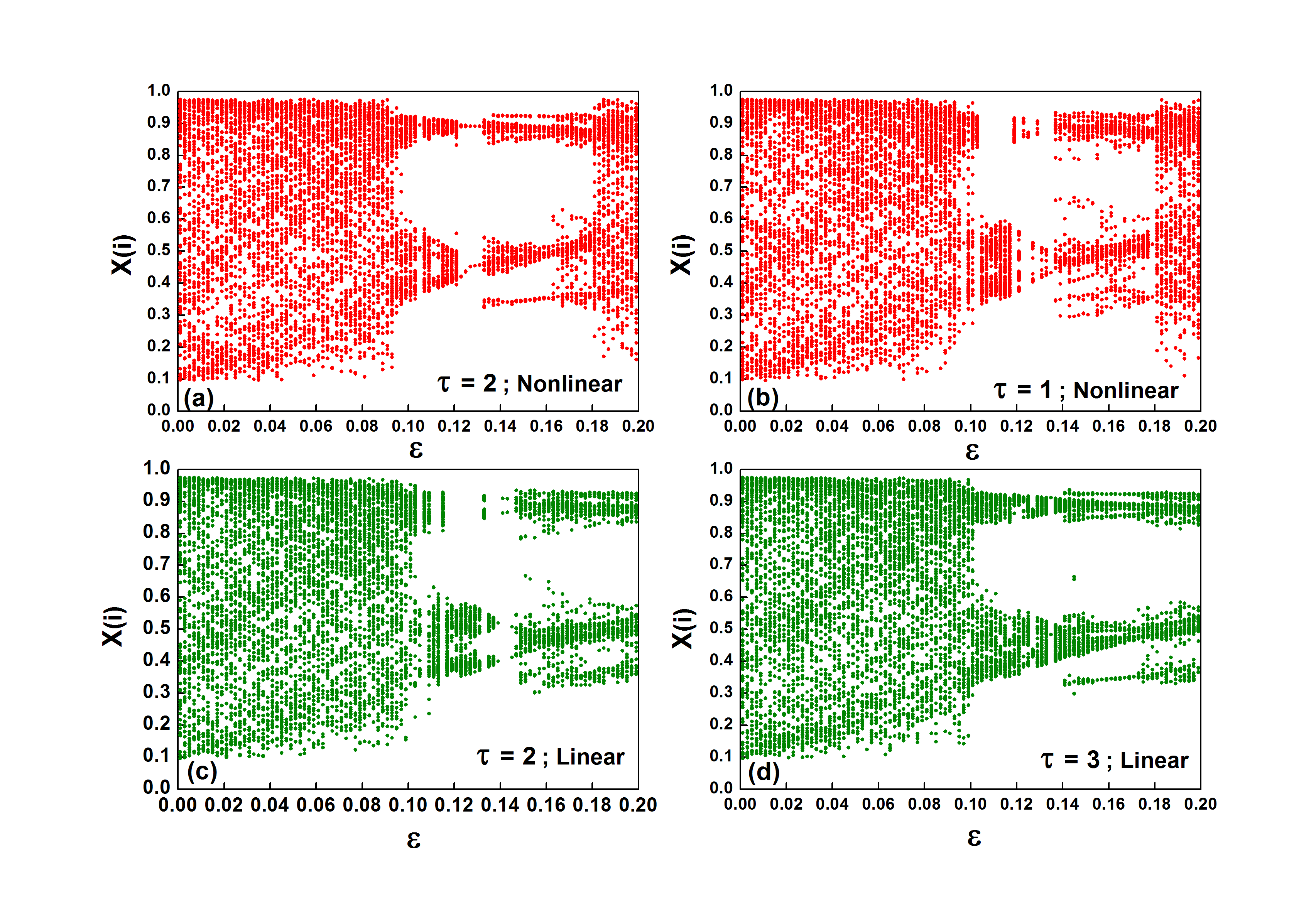
Figure 1: The bifurcation plot is plotted as a function of $x(i)$ versus $\epsilon$ for nonlinear system with delay: (a) $\tau=2$ and (b) $\tau=1$, and for linear system with delay: (c) $\tau=2$ and (d) $\tau=3$. We have shown only representative cases. Similar bifurcation diagrams are obtained for all values of $\tau$.

Now, we decide to assign spin value $s_{i}(t)=1$ (spin-up state) to variable $x_{i}(t)$ if $x_{i}(t)>x^{*}$, and the spin value $s_{i}(t)=-1$ (spin-down state) if $x_{i}(t)<x^{*}$. In other words, the two bands in Fig. 1 correspond to distinct spin states. Initial conditions are random and all sites are in either of the two spin states (that is, the site value are $<x^{*}$, or $\geq x^{*}$) to begin with. When the system is asymptotically stuck in a two-band state (as in a part of $\epsilon>\epsilon_{c}$ region in Fig. 1), we also find that a finite fraction of initial lattice site values have all the time been stuck in their $`$starting-band’ at even times. The spin values at these sites have strictly alternated between $\pm$ during the entire evolution till then. This is called persistence. The values in each part are expected to return to the same part after two applications of the logistic map. We now extend the same expectation to the application of the dynamical equations of Eq.(1) to the CML values. We start with a randomized set of lattice values $x_{i}(0)$ and random past lattice values for the nonzero delay. (The quantitative results on lower critical line do not change much for zero past values.) We examine the spin values at all even time-steps. We say that the site $i$ is persistent till time $t$ if $s_{i}(2t^{{}^{\prime}})=s_{i}(0)$ for all times $t^{{}^{\prime}}$ such that $0\leq t^{{}^{\prime}}\leq t$. In other words, the sites which did not change their spin value even once at all even time-steps are persistent sites. The fraction of such persistent sites, denoted by $P(t)$, is called persistence at time $t$. This definition of persistence derives from local spin persistence. There is a significant part of phase space where the persistence is nonzero. We have shown the values of $\epsilon$ and $\mu$ for which asymptotic value of persistence is nonzero in Fig. 2. We have shown the phase-plot for $\tau=1,2$ for nonlinear coupling and for $\tau=2,3$ for linear coupling. Similar figures are obtained for other values of $\tau$. In this work, we specifically consider the transition to nonzero persistence for $\mu=3.9$ on the lower critical line.

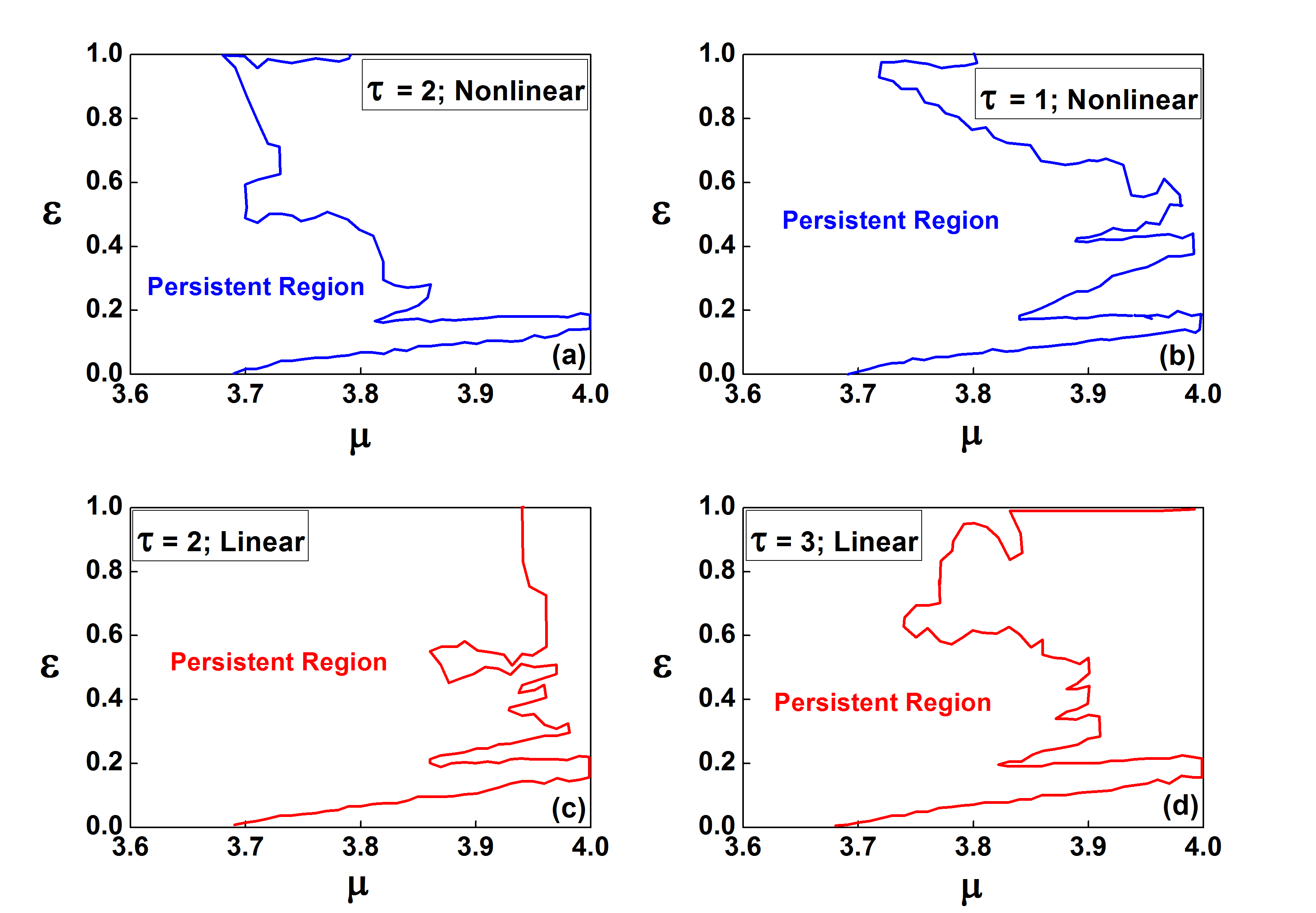
Figure 2: The interface of persistent regions are plotted for nonlinear symmetric coupling for delay: (a) $\tau=2$, and (b) $\tau=1$ and for linear symmetric coupling for delay: (c) $\tau=2$, and (d) $\tau=3$. The approximation by compact region is schematic and there are some persistent points outside the persistent region.

In magnetic systems, the motion of domain walls leads to a ferromagnetic or antiferromagnetic asymptotic state. In one dimension, we do not expect long-range order. However, an interesting behavior emerges on the lower critical line.

Though the temporal behavior of switching between two chaotic bands is common for both types of coupling and any delay, we observe two distinct sub-classes if we take a snapshot of spatial profile in two-band attractor state at the critical point.

In case a), we find that odd and even sublattice are in different bands at a given time step and in case b), all sites in the lattice are in the same band. (See Fig. 3) In both cases, all sites move to other band at next time step and return back to same band after two time steps. They keep returning to the same band at all even times. and make a transition to the other band at all odd times. We call a) and b) as states with antiferromagnetic and ferromagnetic order respectively. Using the above analogy of spin values, we expect that $M(t)=\sum_{i=1}^{N}s_{i}(t)$ acquires a nonzero value in ferromagnetic state while for antiferromagnetic state $M^{\prime}(t)=|\sum_{i=1}^{\frac{N}{2}}(s_{2i}(t)-s_{2i-1}(t))|$ acquires a nonzero value.

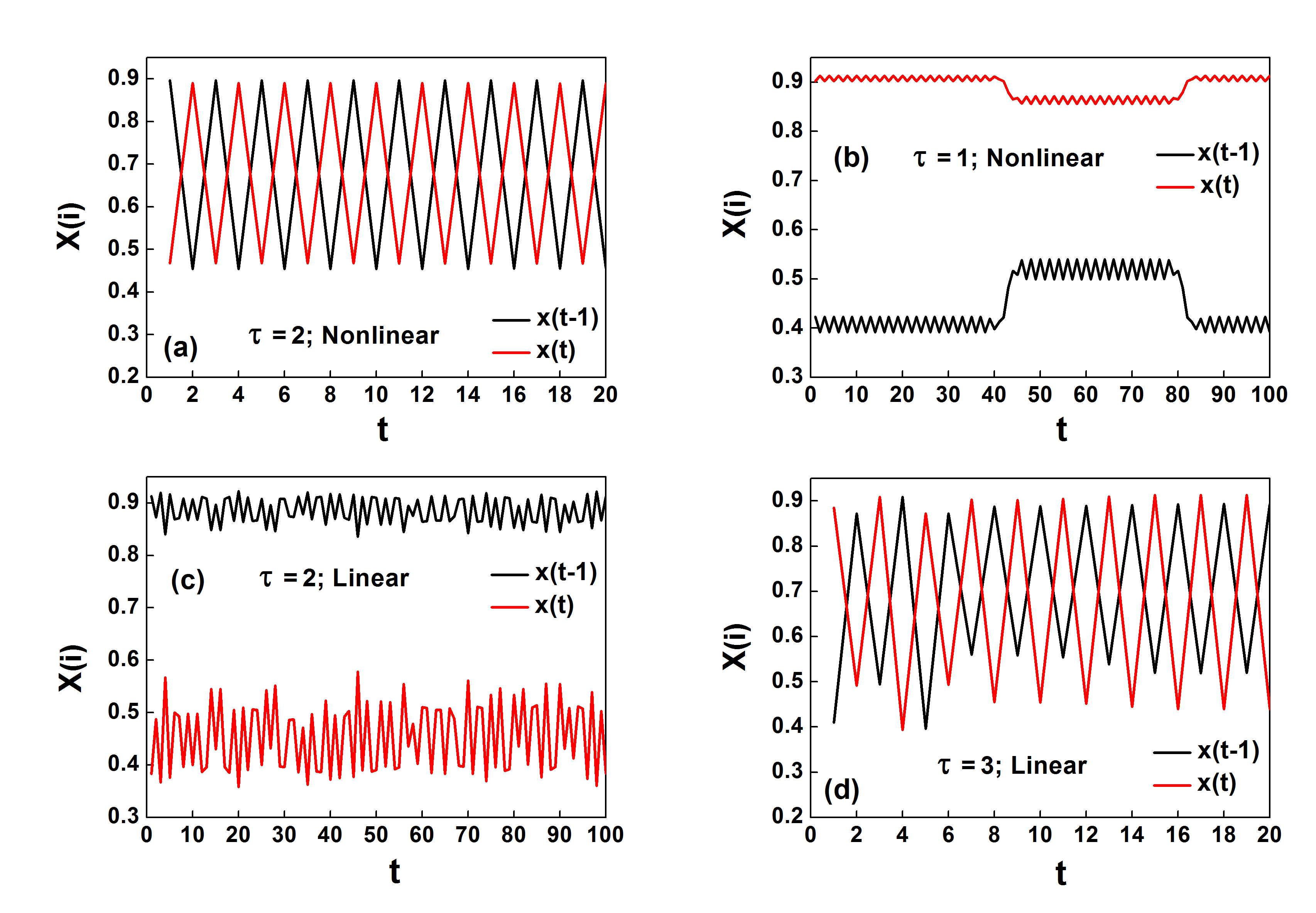
Figure 3: A spatial profile $x_{i}(t)$ (Red colour) and $x_{i}(t-1)$ (Black colour) is plotted as a function of site label $i$ at large $t$ at $\epsilon=\epsilon_{c}$ for (a) nonlinear coupling and $\tau=2$ (b) nonlinear coupling and $\tau=1$ (c) linear coupling and $\tau=2$ and (d) linear coupling and $\tau=3$. We observe a zig-zag, antiferromagnetic pattern in (a) and (d) and all sites are confined to single band in (b) and (c). There are no domain walls and all sites visit another band at next time-step.

Such a state in one dimension will essentially imply the absence of domain walls. A domain wall in one dimension for antiferromagnetic order is appearance of two consecutive like spins. For ferromagnetic order, it is appearance of two consecutive unlike spins. In magnetic systems, the motion of domain walls leads to ferromagnetic or antiferromagnetic order. These walls are expected to undergo random walk and upon meeting each other mutually annihilate thus asymptotically leading to long-range order.

This is precisely the picture for both ferromagnetic and antiferromagnetic ordering, which we observe (See Fig. 4). However, we observe this long-range order at a certain critical point only. Above the critical point, domain walls stop moving and get localized. Below the critical point, they do not freeze. But their number still does not go to zero. The number of domain walls saturates below as well as above the critical point. We investigate the transition from spatiotemporal chaos to this frozen state via a state of long-range order.

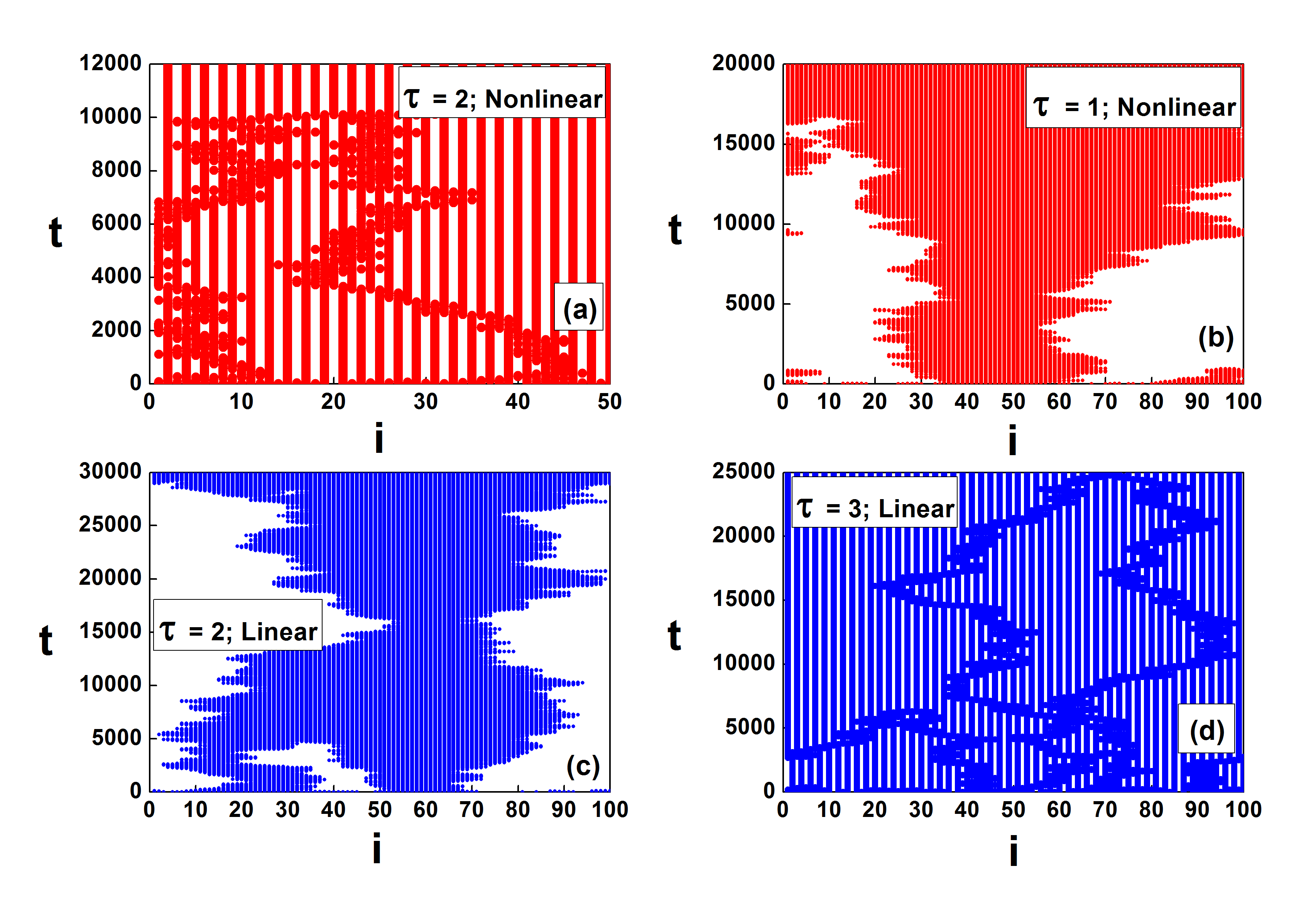
Figure 4: Domain walls motion leading to long range order in one dimension (a) nonlinear coupling, $\tau=2$ (b) nonlinear coupling, $\tau=1$ (c) linear coupling, $\tau=1$ and (d) linear coupling, $\tau=3$. One of the spin values is marked in black. We observe antiferromagnetic ordering for nonlinear coupling with even delay or linear coupling with odd delay. On the other hand, we observe ferromagnetic ordering for nonlinear coupling with odd delay or linear coupling with even delay.

4 Persistence and Domain walls at the critical point

Finding an appropriate order parameter is extremely useful in studies of phase transitions. In our case, we find a single scalar that is nonzero in the phase we are interested in and zero everywhere else. This helps us to distinguish between different phases without having to visually identify them. Also, a quantitative study of such order parameter can give valuable information on the nature of phase transitions.

We study two quantities, i) Density of domain walls and ii) Persistence to quantify the transition. As mentioned above, if $s_{i}(t)\neq s_{i+1}(t)$, we call it a domain wall at site $i$ for ferromagnetic ordering, while for antiferromagnetic ordering, if $s_{i}(t)=s_{i+1}(t)$, we call it a domain wall at site $i$. We expect the order parameter, i.e., density of domain walls to decay as a power-law with exponent 1/2 at the critical point assuming that the comparison with Ising model is valid. This behavior is expected if domain walls undergo random walk and merge upon meeting. This quantity goes to zero at the critical point as a power-law but has a nonzero steady-state value above or below the critical point.

The other quantity persistence, $P(t)$ is the fraction of sites, for each of which the spin at all even times till time $t$ is the same as the initial spin. It has been found useful for studying the transition to fully or partially arrested states in crisis in coupled map lattices.

The non-linear case in Eq.(3) with $\tau=0$, i.e., without delay has been extensively studied by two of us [20], and preliminary investigations on the case with delay are presented in [21]. We extend the study to cases of different delay values as well as those with linear and nonlinear coupling.

Let $\epsilon_{c}$ be the value of coupling at a critical point. We define a critical point $\epsilon_{c}$ as a point such that for $\epsilon<\epsilon_{c}$, the value of $P(t)$ is zero asymptotically. We focus on a critical line of critical points closest to the $\mu$-axis in the phase plots. We plot the behavior of $P(t)$ as a function of $t$ for i) $\epsilon<\epsilon_{c}$ ii) $\epsilon=\epsilon_{c}$ and iii) $\epsilon>\epsilon_{c}$. The persistence goes to zero quickly below the critical point and saturates above the critical point. On the other hand, the density of domain walls $d(t)$ saturates both above and below critical point and shows power-law with exponent close to half only at the critical point. The order parameter can distinguish a phase if it is positive only within the phase and zero outside. In this sense, persistence clearly acts as an order parameter for the crisis state.

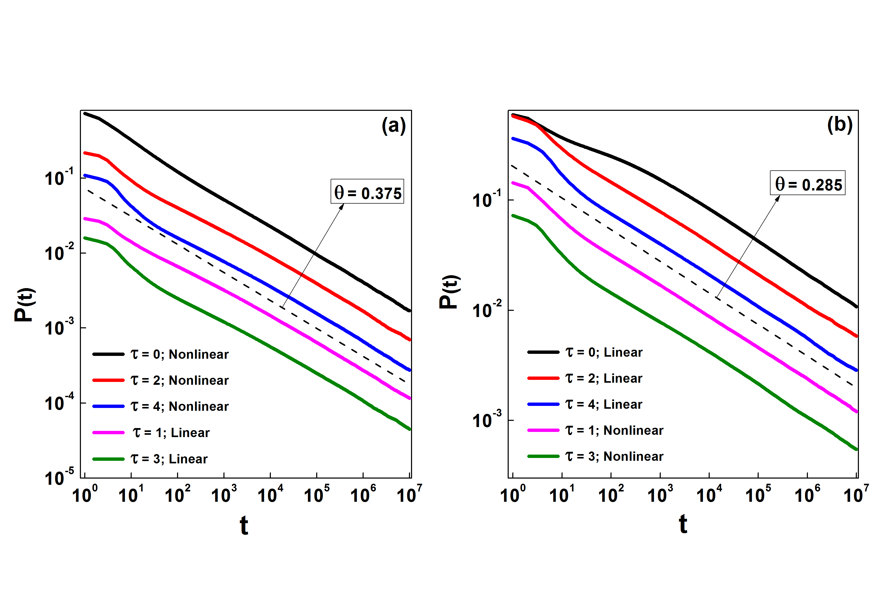
Figure 5: The persistence $P(t)$ is plotted as a function of time $t$ for (a) nonlinear coupling with delay values $\tau=0,2,4$ and linear coupling with delay values $\tau=1,3$ (from top to bottom) and for (b) linear coupling with delay values $\tau=0,2,4$ and nonlinear coupling with delay values $\tau=1,3$ (from top to bottom). The Y-axis values ($P(t)$) are multiplied by arbitrary constant for better visualization. For all cases, $N=10^{5}$. We average over 20 configurations.

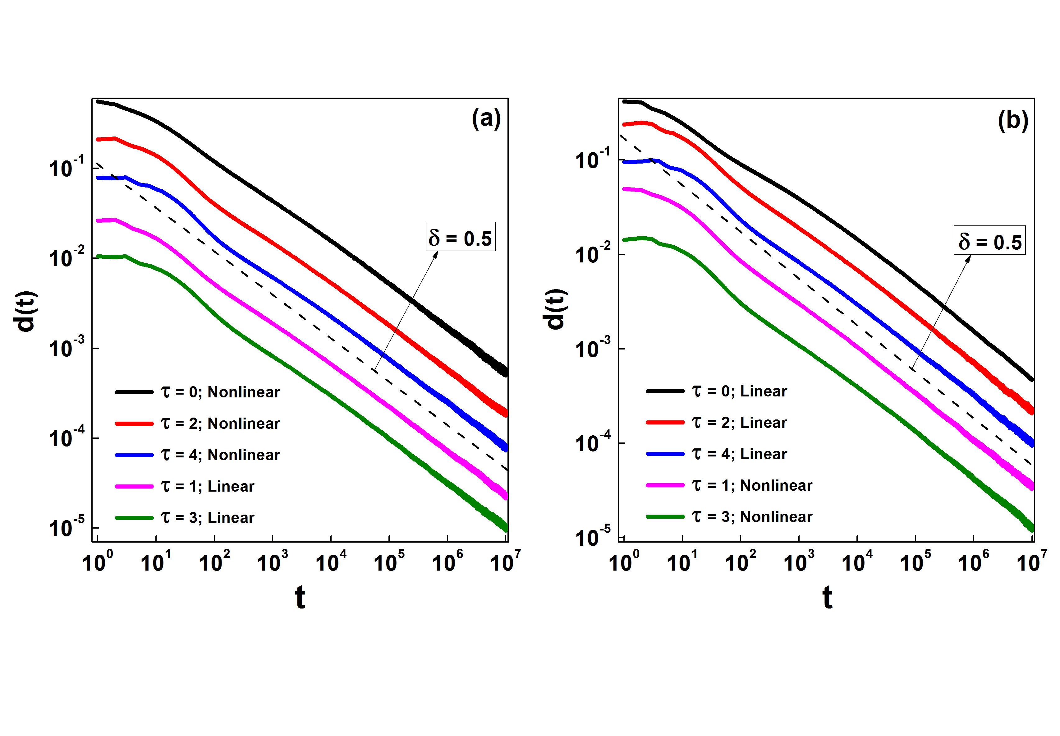
Figure 6: The domain walls $d(t)$ is plotted as a function of time $t$ for (a) nonlinear coupling with delay values $\tau=0,2,4$ and linear coupling with delay values $\tau=1,3$ (from top to bottom) and for (b) linear coupling with delay values $\tau=0,2,4$ and nonlinear coupling with delay values $\tau=1,3$ (from top to bottom). The Y-axis values ($d(t)$) are multiplied by arbitrary constant for better visualization. For all cases, $N=10^{5}$. We average over 20 configurations.

For nonlinear case, we find that i) $\epsilon_{c}=0.11$, for $\tau=0$, ii) $\epsilon_{c}=0.105$, for $\tau=1$, iii) $\epsilon_{c}=0.11$, for $\tau=2$, iv) $\epsilon_{c}=0.11$, for $\tau=3$, and v) $\epsilon_{c}=0.11$, for $\tau=4$. For linear case, we find that i) $\epsilon_{c}=0.115$, for $\tau=0$, ii) $\epsilon_{c}=0.11$, for $\tau=1$, iii) $\epsilon_{c}=0.115$, for $\tau=2$, iv) $\epsilon_{c}=0.11$, for $\tau=3$, and v) $\epsilon_{c}=0.115$, for $\tau=4$. We study the dependence of persistence exponent on delay time and nonlinearity. We observe that the persistence exponent is dependent only on a combination of two factors: a) Nature of coupling: linear, or nonlinear b) delay: odd, or even. For nonlinear coupling and zero or even time-lag, we observe antiferromagnetic ordering. For linear coupling, and odd time-lag, we observe antiferromagnetic ordering. The persistence exponent is ${\frac{3}{8}}=0.375$ for all these cases (See Fig. 5(a)). This is a persistence exponent for Ising model[22]. On the other hand for linear coupling and zero or even time-lag or nonlinear coupling and odd time-lag, we observe ferromagnetic ordering. The persistence exponent is $0.285\sim{\frac{2}{7}}$ in all these cases (See Fig. 5(b)). Thus the system shows remarkable universality despite extensions introduced in the model. The number of domain walls decays with an exponent close to $1/2$ in all these cases (See Fig. 6(a) and 6(b)).

The comparison with Ising model dynamics in one dimension is very appropriate since ${\frac{3}{8}}$ is Ising-type persistence exponent for antiferromagnetic order[22]. The behavior described above could be understood as follows: The motivation for defining persistence based on a modulo 2 (rather than modulo 1!) dynamics was that a single application of logistic map flips the spin state of a typical lattice site and a double application typically retains the spin state. (The slope $f^{\prime}(x^{*})$ at unstable fixed point $x^{*}$ is negative.) However, (i) since there is a finite probability that a spin down state does not change to a spin-up state under logistic map, and (ii) since the dynamical equations also involve other terms like the coupling, clearly, retention of spin state will not happen for a certain non-zero fraction of sites. Thus, if the lattice or a part of it is stuck in 2-band attractor state, a certain fraction of sites will not flip spin even asymptotically at each modulo 2 dynamical-step. If it is not stuck in 2-band state, every site will eventually flip leading to zero persistence. At the critical point or below it, we observe the decay of persistence with time.

The nature of this decay is expected to depend on parameters of the system such as the coupling strength and the time lag. Our computation shows that coupling with the logistic map (i.e. non-linear coupling) acts as an effective negative spin-coupling for the lattice for long-time evolution. The dynamics, as well as qualitative features are then similar to the Ising model. Linear coupling is like coupling with the identity map and it acts as positive coupling. Long-range ordering in this system is different and so is persistence exponent. Since the coupling is small, value of $x_{i-1}(t)$ is close to $f(x_{i-1}(t-1))$. Thus linear coupling without delay is similar to nonlinear coupling with $\tau=1$. Thus a nonlinear system with delay $\tau=1$ acts like linear system without delay. With even delay, the map is iterated even number of times. For nonlinear coupling, with zero delay, the bands tend to alternate since $f^{\prime}(x^{*})$ is negative. For $\tau=1$, the inverse image of map with two iterations is of interest. The sign of $f^{\prime}(x^{*})$ is same as sign of $f^{-1^{\prime}}(x^{*})$. (Because $dy/dx={\frac{1}{(dx/dy)}}$). Since $x^{*}$ is a fixed point, $f^{(\tau+1)^{\prime}}(x^{*})=(f^{\prime}(x^{*}))^{(\tau+1)}$, and its sign is negative for even delay and positive for odd delay. So the system with even delay acts like system with no delay for nonlinear coupling. As we argued above, system with odd delay and nonlinear coupling is like system with even delay and linear coupling. Thus, coupling to delayed lattice value with odd delay can convert a positive spin-coupling to a negative one and conversely.

Therefore, in general, non-linear coupling with even delays stabilizes, and grows subsets of sites in which the neighboring sites are in different bands, i.e., have values on opposite sides of $x^{*}$. The same is true for linear coupling with odd delays. Similarly, non-linear coupling with odd delays, as well as linear coupling with even delays, stabilize and grows subsets with neighboring sites in the same band. Though we can thus qualitatively decipher the ferro or antiferro ordering with these hand-waving arguments, it is a surprise that it turns out so well for all values of delay $\tau$ studied by us from $\tau=0$ to 4.

5 System with asymmetry

So far, we have studied the system at $D=0$ in Eqs. 5 and 6. The phase plots do not change much in the presence of small asymmetry. However, the disturbances move towards left or right and persistence decays faster. There is no well-defined persistence exponent at the critical point. The persistence may decay as stretched exponential or exponential. For example, for $\tau=1$ and $\tau=2$ and $D=0.05\epsilon$, we observe stretched exponential decay of persistence at critical point for nonlinear coupling. (See Fig. 7). In this case $P(t)\sim\exp(-rt^{0.5})$. However, the behavior depends on asymmetry and delay. The behavior at the critical point is not uniform at all critical points in the presence of asymmetry.

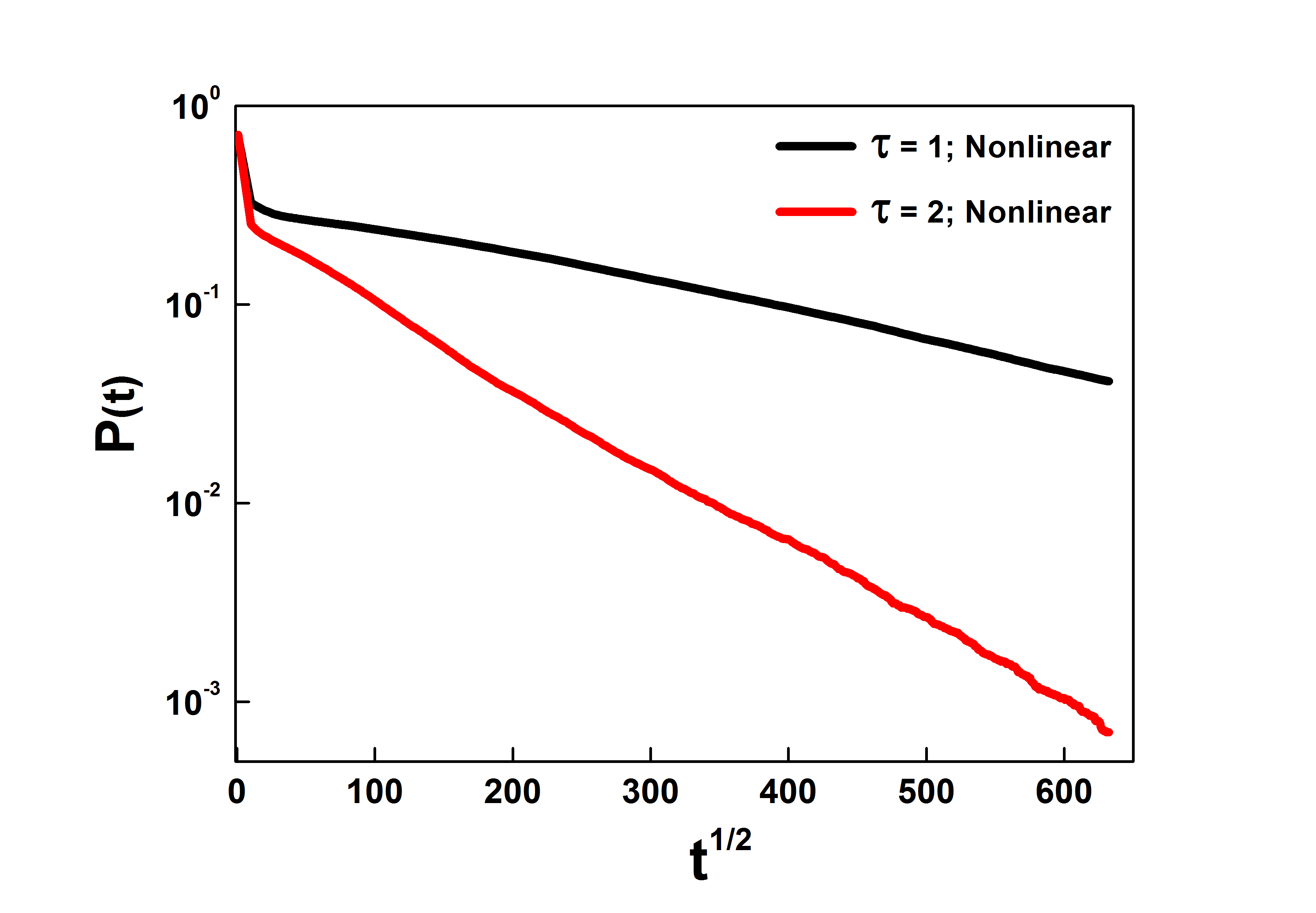
Figure 7: The stretched exponential decay is observed with exponent $0.5$ for nonlinear coupling with $\tau=1$ ($\epsilon_{c}=0.1423$) and $\tau=2$ ($\epsilon_{c}=0.1355$) and $D=0.05\epsilon$.

6 Discussion

In all cases of symmetric coupling discussed above, as the critical line is crossed, we obtain a transition to a state with long-range ferromagnetic, or antiferromagnetic order. We conclude that linear coupling with zero or even delay acts like ferromagnetic coupling, whereas, nonlinear coupling with zero, or even delay acts like antiferromagnetic coupling. On the other hand, linear coupling with odd delay leads to antiferromagnetic order, and nonlinear coupling with odd delay leads to ferromagnetic order. Also, on the critical line time-decay of persistence is governed by a power-law. For antiferromagnetic order, persistence exponent is $\approx 3/8$ while for ferromagnetic order the persistence exponent is $\approx 2/7$.

These results are surprising for the two reasons a) Persistence exponents are known to change with detailed dynamics of the system. But the exponents take only two values depending on the asymptotic state. b) The exponent $0.375$ is obtained for antiferromagnetic order. This exponent $0.375$ is reported for the Ising model. It is interesting that, for all cases with antiferromagnetic order, the same exponent is obtained. This underlines the similarity of coupled logistic maps with nonlinear coupling with Ising model. Surprisingly, the exponent changes for the system leading to ferromagnetic order. For the 1-d Ising model, the system with negative coupling $J$ can be mapped to the system with positive coupling by changing the sign of spins of one of the sub-lattices. Thus there is no real difference in these two cases for the Ising model. However, we obtain Ising-like exponents only when there is antiferromagnetic order asymptotically. The exponent in the other case is also universal. Nevertheless, it is not reported before.

In presence of asymmetry, there is no universal behavior at the critical point. The decay is faster than power-law. However, the detailed behavior depends on specific parameters such as the strength of asymmetry.

References

- [1] G. Jaeger, The Ehrenfest classification of phase transitions: introduction and evolution, Arch. Hist. Exact Sci. 53 (1) (1998) 51–81.
- [2] O. C. Martin, R. Monasson, R. Zecchina, Statistical mechanics methods and phase transitions in optimization problems, Theor. Comput. Sci. 265 (1-2) (2001) 3–67.
- [3] K. Kaneko, Period-doubling of kink-antikink patterns, quasiperiodicity in antiferro-like structures and spatial intermittency in coupled logistic lattice: Towards a prelude of a “field theory of chaos”, Prog. Theor. Phys. 72 (3) (1984) 480–486.
- [4] A. C. Marti, C. Masoller, Delay-induced synchronization phenomena in an array of globally coupled logistic maps, Phys. Rev. E 67 (5) (2003) 056219.
- [5] C. Masoller, A. C. Marti, Random delays and the synchronization of chaotic maps, Phys. Rev. Lett. 94 (13) (2005) 134102.
- [6] F. M. Atay, J. Jost, A. Wende, Delays, connection topology, and synchronization of coupled chaotic maps, Phys. Rev. Lett. 92 (14) (2004) 144101.
- [7] B. Derrida, A. J. Bray, C. Godreche, Non-trivial exponents in the zero temperature dynamics of the 1d Ising and Potts models, J. Phys. A: Math. Gen. 27 (11) (1994) L357.
- [8] A. Lemaître, H. Chaté, Phase ordering and onset of collective behavior in chaotic coupled map lattices, Phys. Rev. Lett. 82 (6) (1999) 1140.
- [9] J. Kockelkoren, A. Lemaître, H. Chaté, Phase-ordering and persistence: relative effects of space-discretization, chaos, and anisotropy, Physica A 288 (1-4) (2000) 326–337.
- [10] K. Tucci, M. G. Cosenza, O. Alvarez-Llamoza, Phase separation in coupled chaotic maps on fractal networks, Phys. Rev. E 68 (2) (2003) 027202.
- [11] Z. Jabeen, N. Gupte, Universality classes of spatiotemporal intermittency, Physica A 384 (1) (2007) 59–63.
- [12] J. Miller, D. A. Huse, Macroscopic equilibrium from microscopic irreversibility in a chaotic coupled-map lattice, Phys. Rev. E 48 (4) (1993) 2528.
- [13] P. Marcq, H. Chaté, P. Manneville, Universality in Ising-like phase transitions of lattices of coupled chaotic maps, Phys. Rev. E 55 (3) (1997) 2606.
- [14] Y. Oono, S. Puri, Study of phase-separation dynamics by use of cell dynamical systems. I. Modeling, Phys. Rev. A 38 (1) (1988) 434.
- [15] E. Salazar-Neumann, M. C. Vargas, G. Pérez, Critical behavior of a dynamic analog to the q= 3 Potts model, Phys. Rev. E 71 (3) (2005) 036228.
- [16] A. V. Mahajan, P. M. Gade, Transition from clustered state to spatiotemporal chaos in a small-world networks, Phys. Rev. E 81 (5) (2010) 056211.
- [17] A. R. Sonawane, P. M. Gade, Dynamic phase transition from localized to spatiotemporal chaos in coupled circle map with feedback, Chaos 21 (1) (2011) 013122.
- [18] A. V. Mahajan, P. M. Gade, Stretched exponential dynamics of coupled logistic maps on a small-world network, J. Stat. Mech.: Theory Exp. 2018 (2) (2018) 023212.
- [19] K. Kaneko, Spatial period-doubling in open flow, Phys. Lett. A 111 (7) (1985) 321–325.
- [20] P. M. Gade, G. G. Sahasrabudhe, Universal persistence exponent in transition to antiferromagnetic order in coupled logistic maps, Phys. Rev. E 87 (5) (2013) 052905.
- [21] B. P. Rajvaidya, G. G. Sahasrabudhe, P. M. Gade, Universal exponents at critical line pertaining to second order phase transition in coupled logistic maps, in: AIP Conf. Proc., Vol. 2104, AIP Publishing LLC, 2019, p. 030025.
- [22] B. Derrida, V. Hakim, V. Pasquier, Exact exponent for the number of persistent spins in the zero-temperature dynamics of the one-dimensional Potts model, J. Stat. Phys. 85 (5-6) (1996) 763–797.