On explicit form of the FEM stiffness matrix for the integral fractional Laplacian on non-uniform meshes

Abstract.

We derive exact form of the piecewise-linear finite element stiffness matrix on general non-uniform meshes for the integral fractional Laplacian operator in one dimension, where the derivation is accomplished in the Fourier transformed space. With such an exact formulation at our disposal, we are able to numerically study some intrinsic properties of the fractional stiffness matrix on some commonly used non-uniform meshes (e.g., the graded mesh), in particular, to examine their seamless transition to those of the usual Laplacian.

1. Introduction

There has been a burgeoning of recent interest in nonlocal and fractional models, largely due to the advancement in both computing power and computational algorithms. The integral fractional Laplacian (IFL) is deemed as one of the most prominent nonlocal operators, but unfortunately, it poses more challenges in numerical solutions of the related models. Among very limited works on finite element approximation of the IFL, D’Elia and Gunzburger [2] considered the FEM discretisation on non-uniform meshes in one dimension. The entries of the FEM stiffness matrix therein were computed by the Gauss quadrature rule, and the adaptive Gauss–Kronrod quadrature (with a built-in function in Matlab) was resorted to approximate the double integrals with singular kernels when the mesh size is small.

In this paper, we compute the entries of the stiffness matrix in the Fourier transformed space based on the definition of the IFL: for $s\geq 0,$

$$\begin{split}&(-\Delta)^{s}u(x):={\mathscr{F}}^{-1}\big{[}|\xi|^{2s}{\mathscr{F}}[u](\xi)\big{]}(x),\end{split}$$ (1)

where $u(x)$ on $\mathbb{R}=(-\infty,\infty)$ is of Schwartz class, and $\mathscr{F}$ denotes the Fourier transform with the inverse ${\mathscr{F}}^{-1}.$ In fact, for $s\in(0,1),$ the IFL of $u(x)$ can be equivalently defined by

$$(-\Delta)^{s}u(x)=C_{s}\,{\rm p.v.}\!\int_{\mathbb{R}}\frac{u(x)-u(y)}{|x-y|^{1+2s}}{\rm d}y\;\;\;\;\text{with}\quad C_{s}=\frac{2^{2s}s\,\Gamma(s+\frac{1}{2})}{\sqrt{\pi}\,\Gamma(1-s)},$$ (2)

where “p.v.” stands for the principle value and $\Gamma(\cdot)$ in the Gamma function. As opposed to [2] and limited existing works implemented via (2), the use of the formulation (1) enables us to evaluate the entries explicitly. With such an analytic representation, we can study some intrinsic properties of the stiffness matrix and related numerical issues when the meshes are highly non-uniform.

2. Main result

Consider the model equation with a global homogeneous Dirichlet boundary condition:

$$(-\Delta)^{s}u(x)=f(x),\quad x\in\Omega=(a,b);\quad u(x)=0,\quad x\in\Omega^{c}=\mathbb{R}\backslash\bar{\Omega},$$ (3)

where $f(x)$ is a given continous function. Let $\{\phi_{j}(x)\}_{j=1}^{N-1}$ be the piecewise linear finite element basis (i.e., the standard “hat” functions) associate with the partition

$$\Omega:\;\;a=x_{0}<x_{1}<\cdots<x_{N}=b,$$ (4)

and satisfy $\phi_{j}(x)\equiv 0$ for $x\in\Omega^{c}$. The piecewise linear FEM approximation to (3) is to find $u_{h}\in V_{h}^{0}={\rm span}\{\phi_{j}\,:\,1\leq j\leq N-1\}$ such that

$$a_{s}(u_{h},v_{h})=\int_{\mathbb{R}}((-\Delta)^{s/2}u_{h})((-\Delta)^{s/2}v_{h}){\rm d}x=\int_{\Omega}f(x)v_{h}(x)\,{\rm d}x,\quad\forall\,v_{h}\in V_{h}^{0},$$ (5)

which admits a unique solution by the standard Lax-Milgram lemma.

2.1. Main result

Our main purpose is to show that the stiffness matrix, denoted by $\bm{S},$ with the entries

$$S_{kj}=S_{jk}=a_{s}(\phi_{j},\phi_{k}),\quad 1\leq k,j\leq N-1,$$

has the following explicit form.

Theorem 1.

If $s\in(0,3/2)$ but $s\not=1/2,$ then the entries of the stiffness matrix $\bm{S}$ can be explicitly evaluated by

$$S_{jk}=\widehat{C}_{s}\,{\bm{c}_{j}\,\bm{D}^{k}_{j}\,\bm{c}_{k}^{t}}\;\;\;\;{\rm with}\;\;\;\widehat{C}_{s}:=\frac{1}{2\Gamma(4-2s)\cos(s\pi)},$$ (6)

where

$$\begin{split}&\bm{c}_{l}=\Big{(}\frac{1}{h_{l}},-\frac{1}{h_{l}}-\frac{1}{h_{l+1}},\frac{1}{h_{l+1}}\Big{)},\quad\bm{D}^{k}_{j}=\!\begin{pmatrix}(d^{k-1}_{j-1})^{\gamma}&(d^{k}_{j-1})^{\gamma}&(d^{k+1}_{j-1})^{\gamma}\\[6.0pt] (d^{k-1}_{j})^{\gamma}&(d^{k}_{j})^{\gamma}&(d^{k+1}_{j})^{\gamma}\\[6.0pt] (d^{k-1}_{j+1})^{\gamma}&(d^{k}_{j+1})^{\gamma}&(d^{k+1}_{j+1})^{\gamma}\end{pmatrix},\end{split}$$ (7)

with $h_{\ell}=x_{\ell}-x_{\ell-1},$ $d_{\iota}^{\ell}=|x_{\iota}-x_{\ell}|,$ and $\gamma=3-2s.$

If $s=1/2$, then we have

$$S_{jk}=\frac{1}{2\pi}\bm{c}_{j}\begin{pmatrix}(d^{k-1}_{j-1})^{2}\ln d^{k-1}_{j-1}&(d^{k}_{j-1})^{2}\ln d^{k}_{j-1}&(d^{k+1}_{j-1})^{2}\ln d^{k+1}_{j-1}\\[6.0pt] (d^{k-1}_{j})^{2}\ln d^{k-1}_{j}&(d^{k}_{j})^{2}\ln d^{k}_{j}&(d^{k+1}_{j})^{2}\ln d^{k+1}_{j}\\[6.0pt] (d^{k-1}_{j+1})^{2}\ln d^{k-1}_{j+1}&(d^{k}_{j+1})^{2}\ln d^{k}_{j+1}&(d^{k+1}_{j+1})^{2}\ln d^{k+1}_{j+1}\end{pmatrix}\bm{c}_{k}^{t},$$ (8)

where we understand $(d^{\ell}_{\iota})^{2}\ln d^{\ell}_{\iota}=0$ when $d^{\ell}_{\iota}=0.$

Prior to the proof, we discuss some implications and consequences of the main result. Observe from the above that for fixed $s\in(0,3/2),$ the matrix $\bm{S}$ is completely determined by the partition (4), and for fixed $j,k$, the entry $S_{jk}$ only involves the grid points: $\{x_{j+p}\}_{p=0,\pm 1}$ and $\{x_{k+q}\}_{q=0,\pm 1}.$ Interestingly, $S_{jk}$ turns out be a finite difference approximation of

$$\hat{d}(x,y)=\widehat{C}_{s}\,|x-y|^{3-2s},\;\;{\rm if}\;\;s\not=\frac{1}{2};\quad\hat{d}(x,y)=\frac{1}{2\pi}(x-y)^{2}\ln|x-y|,\;\;{\rm if}\;\;s=\frac{1}{2}.$$

Indeed, one verifies from Theorem 1 the following alternative representation.

Corollary 1.

For $s\in(0,3/2),$ the entry $S_{jk}$ can be written as a finite difference form

$$S_{jk}=\delta_{y}^{2}\delta_{x}^{2}\hat{d}_{j}^{k}=\delta_{x}^{2}\delta_{y}^{2}\hat{d}_{j}^{k},\quad 1\leq j,k\leq N-1,$$ (9)

where $\hat{d}_{j}^{k}=\hat{d}(x_{j},x_{k})$ and

$$\delta_{x}^{2}\hat{d}_{j}^{k}:=\frac{\hat{d}_{j}^{k}-\hat{d}_{j-1}^{k}}{h_{j}}-\frac{\hat{d}_{j+1}^{k}-\hat{d}_{j}^{k}}{h_{j+1}},\quad\delta_{y}^{2}\hat{d}_{j}^{k}:=\frac{\hat{d}_{j}^{k}-\hat{d}_{j}^{k-1}}{h_{k}}-\frac{\hat{d}_{j}^{k+1}-\hat{d}_{j}^{k}}{h_{k+1}}.$$

Remark 1.

It is noteworthy that from standard finite difference formula, we have

$$\delta_{x}^{2}\hat{d}_{j}^{k}=\frac{1}{2}(h_{j}+h_{j+1})\partial_{x}^{2}\hat{d}(x_{j},x_{k})+O(h_{j}^{2}+h_{j+1}^{2}).$$ (10)

Thus, $S_{jk}$ is a nine-point finite difference approximate of $\hat{d}(x,y)$ on $\{(x_{j+p},x_{k+q})\}_{p,q=0,\pm 1}.$ ∎

Remark 2.

When $s\to 0$ and $s=1$, the matrix $\bm{S}$ in Theorem 1 reduces to the usual (tridiagonal) FEM mass matrix $\bm{M}={\rm diag}(h_{j}/6,(h_{j}+h_{j+1})/3,h_{j+1}/6)$ and the stiffness matrix $\bm{S}={\rm diag}(-1/h_{j},1/h_{j}+1/h_{j+1},-1/h_{j+1})$, respectively. If (4) is a uniform partition of $(a,b)$ with $h=h_{j}$, then (6) reduces to

$$S_{jk}=\widehat{C}_{s}{h^{1-2s}}\sum_{i=-2}^{2}w_{i}\big{|}|k-j|+i\big{|}^{3-2s}\;\;{\rm with}\;\;w_{0}=6,\;\;w_{\pm 1}=-4,\;\;w_{\pm 2}=1.$$

In this case, the stiffness matrix $\bm{S}$ is a Toeplitz matrix (cf. [7] and also for some other interesting properties). ∎

2.2. Proof of Theorem 1

Recap on the piecewise linear FEM basis associated with (4):

$$\phi_{j}(x)=\begin{cases}c_{j}(x-x_{j-1}),\quad&x\in(x_{j-1},x_{j}),\\ c_{j+1}(x_{j+1}-x),\quad&x\in(x_{j},x_{j+1}),\\ 0,\quad&\text{elsewhere on}\,\,\mathbb{R},\end{cases}\quad c_{\ell}=\frac{1}{h_{\ell}},$$ (11)

for $1\leq j\leq N-1.$ Using integration by parts leads to

$$\mathscr{F}[\phi_{j}](\xi) =\frac{1}{\sqrt{2\pi}}\int_{\mathbb{R}}\phi_{j}(x)e^{-{\rm i}x\xi}\,{\rm d}x=\frac{1}{\sqrt{2\pi}}\int_{x_{j-1}}^{x_{j+1}}\phi_{j}(x)e^{-{\rm i}x\xi}\,{\rm d}x$$ (12)

$$=\frac{c_{j}}{\sqrt{2\pi}}\int_{x_{j-1}}^{x_{j}}(x-x_{j-1})e^{-{\rm i}x\xi}\,{\rm d}x+\frac{c_{j+1}}{\sqrt{2\pi}}\int_{x_{j}}^{x_{j+1}}(x_{j+1}-x)e^{-{\rm i}x\xi}\,{\rm d}x$$

$$=\frac{1}{\sqrt{2\pi}}\Big{[}\frac{c_{j}}{\xi^{2}}(e^{-{\rm i}x_{j}\xi}-e^{-{\rm i}x_{j-1}\xi})-\frac{c_{j+1}}{\xi^{2}}(e^{-{\rm i}x_{j+1}\xi}-e^{-{\rm i}x_{j}\xi})\Big{]}$$

$$=-\frac{1}{\sqrt{2\pi}}\frac{c_{j}e^{-{\rm i}x_{j-1}\xi}-(c_{j}+c_{j+1})e^{-{\rm i}x_{j}\xi}+c_{j+1}e^{-{\rm i}x_{j+1}\xi}}{\xi^{2}}=-\frac{1}{\sqrt{2\pi}\xi^{2}}\bm{c}_{j}\bm{e}_{j}(\xi),$$

where $\bm{e}_{j}(\xi):=(e^{-{\rm i}x_{j-1}\xi},e^{-{\rm i}x_{j}\xi},e^{-{\rm i}x_{j+1}\xi})^{t}.$ In view of (1), (5), and (12), we obtain from direct calculation and the parity of cosines and sines that

$$\begin{split}S_{jk}&=\int_{\mathbb{R}}|\xi|^{2s}\mathscr{F}[\phi_{j}](\xi)\overline{\mathscr{F}[\phi_{k}](\xi)}\,{\rm d}\xi=\frac{1}{2\pi}\bm{c}_{j}\Big{(}\int_{\mathbb{R}}|\xi|^{2s-4}\bm{e}_{j}(\xi)\bm{e}_{k}^{t}(-\xi){\rm d}\xi\Big{)}\bm{c}_{k}^{t}\\ &=\frac{1}{\pi}\int_{0}^{\infty}\xi^{2s-4}f_{jk}(\xi)\,{\rm d}\xi,\end{split}$$ (13)

where

$$f_{jk}(\xi)=\bm{c}_{j}\bm{F}_{jk}(\xi)\bm{c}_{k}^{t},\quad\bm{F}_{jk}(\xi)=\begin{pmatrix}\cos(d_{j-1}^{k-1}\xi)&\cos(d_{j-1}^{k}\xi)&\cos(d_{j-1}^{k+1}\xi)\\[2.0pt] \cos(d_{j}^{k-1}\xi)&\cos(d_{j}^{k}\xi)&\cos(d_{j}^{k+1}\xi)\\[2.0pt] \cos(d_{j+1}^{k-1}\xi)&\cos(d_{j+1}^{k}\xi)&\cos(d_{j+1}^{k+1}\xi)\end{pmatrix}.$$

One verifies from direct calculation or finite difference approximation (cf. (9) and (10)) that $f_{jk}(0)=f^{\prime}_{jk}(0)=f^{\prime\prime}_{jk}(0)=0.$

We first consider $s\in(1,3/2)$. Recall the integral identity (cf. [5, p. 440]):

$$\int^{\infty}_{0}x^{\mu-1}\sin(ax)\,{\rm d}x=\frac{\Gamma(\mu)}{a^{\mu}}\sin\Big{(}\frac{\mu\pi}{2}\Big{)},\quad a>0,\;\;\mu\in(0,1).$$ (14)

We derive from (13) and integration by parts that

$$\int_{0}^{\infty} \xi^{2s-4}f_{jk}(\xi)\,{\rm d}\xi=\frac{1}{2s-3}\Big{\{}\xi^{2s-3}f_{jk}(\xi)\big{|}_{0}^{\infty}-\int_{0}^{\infty}\xi^{2s-3}f^{\prime}_{jk}(\xi)\,{\rm d}\xi\Big{\}}$$ (15)

$$=-\frac{1}{2s-3}\int_{0}^{\infty}\xi^{2s-3}f^{\prime}_{jk}(\xi)\,{\rm d}\xi=-\frac{1}{2s-3}\bm{c}_{j}\Big{(}\int_{0}^{\infty}\xi^{2s-3}\bm{F}^{\prime}_{jk}(\xi){\rm d}\xi\Big{)}\bm{c}_{k}^{t}.$$

Applying (14) with $\mu=2s-2$ to each entry of $\xi^{2s-3}\bm{F}^{\prime}_{jk}(\xi)$ yields

$$\int_{0}^{\infty}\xi^{2s-4}f_{jk}(\xi)\,{\rm d}\xi=-\Gamma(2s-3)\sin(s\pi)\,{\bm{c}_{j}\bm{D}^{k}_{j}\bm{c}_{k}^{t}}.$$

We next consider $s\in(1/2,1).$ Recall that (cf. [5, p. 441])

$$\int_{0}^{\infty}x^{\mu-1}\cos(ax){\rm d}x=\frac{\Gamma(\mu)}{a^{\mu}}\cos\Big{(}\frac{\mu\pi}{2}\Big{)},\quad a>0,\;\mu\in(0,1).$$ (16)

Applying integration by parts one more time to (15), we derive from (16) with $\mu=2s-1$ that

$$\int_{0}^{\infty}\xi^{2s-4}f_{jk}(\xi)\,{\rm d}\xi =\frac{1}{(2s-3)(2s-2)}\int_{0}^{\infty}\xi^{2s-2}f^{\prime\prime}_{jk}(\xi)\,{\rm d}\xi$$ (17)

$$=\frac{1}{(2s-3)(2s-2)}\bm{c}_{j}\Big{(}\int_{0}^{\infty}\xi^{2s-2}\bm{F}^{\prime\prime}_{jk}(\xi){\rm d}\xi\Big{)}\bm{c}_{k}^{t}$$

$$=-\Gamma(2s-3)\sin(s\pi)\,{\bm{c}_{j}\bm{D}^{k}_{j}\bm{c}_{k}^{t}}.$$

We now turn to $s\in(0,1/2)$. Similarly, we integrate (17) by parts once more and use (14) with $\mu=2s$ to obtain

$$\int_{0}^{\infty}\xi^{2s-4}f_{jk}(\xi){\rm d}\xi =-\frac{1}{(2s-3)(2s-2)(2s-1)}\int_{0}^{\infty}\xi^{2s-1}f^{\prime\prime\prime}_{jk}(\xi){\rm d}\xi$$

$$=-\Gamma(2s-3)\sin(s\pi)\,{\bm{c}_{j}\bm{D}^{k}_{j}\bm{c}_{k}^{t}}.$$

Then, using the property: $\Gamma(z)\Gamma(1-z)=\pi/{\sin\pi z}$ ($z\not=0,-1,\cdots$), we can reformulate the constant and then obtain the desired representation in (6) for all three cases.

Finally, for $s=1/2,$ using the fact and the basic limit

$$\lim_{s\to\frac{1}{2}}\textbf{c}_{j}\bm{D}_{j}^{k}\textbf{c}_{k}^{t}=0,\quad\ln z=\lim_{\delta\to 0}\frac{z^{\delta}-1}{\delta},\;\;\;z>0,$$

we can directly take limit on (6):

$$S_{jk}=\frac{1}{4}\lim_{s\to\frac{1}{2}}\frac{\bm{c}_{j}\bm{D}_{j}^{k}\bm{c}_{k}^{t}}{\cos(s\pi)},$$

and use the L’Hospital’s rule to obtain (8). This completes the proof.

3. FEM on graded meshes

It is known that the graded meshes are commonly used in finite element approximation of solutions with boundary singularities. In general, the mesh geometry affects not only the approximation error of the finite element solution but also the spectral properties of the corresponding stiffness matrix. It is a well-studied topic in the integer-order case, but much less known in this fractional setting.

3.1. A singular mapping

We propose to generate the graded mesh on $[a,b]$ for the solutions with singularities at the endpoint(s) by the singular mapping [9]:

$$x=g(y;\alpha,\beta)=a+(b-a)\frac{B(y;\alpha,\beta)}{B(\alpha,\beta)}\;\;\;{\rm with}\;\;\;B(y;\alpha,\beta)=\int_{0}^{y}t^{\alpha-1}(1-t)^{\beta-1}{\rm d}t,$$ (18)

for $y\in[0,1],x\in[a,b],$ and $\alpha,\beta\geq 1,$ where $B(y,\alpha,\beta)$ is incomplete Beta function and $B(\alpha,\beta)=B(1;\alpha,\beta)$ is the Beta function. It is a one-to-one mapping such that $a=g(0;\alpha,\beta)$ and $b=g(1;\alpha,\beta).$ If $\alpha=\beta=1,$ it reduces to a linear transform. Let $\{y_{j}=j/N\}_{j=0}^{N}$ be a uniform partition of the reference interval $[0,1].$ Then the mapped grids on $[a,b]$ are given by

$$x_{j}:=x_{N,j}^{(\alpha,\beta)}=g(y_{j};\alpha,\beta)=g(j/N;\alpha,\beta),\quad 0\leq j\leq N.$$ (19)

By the mean value theorem,

$$h_{j}=x_{j}-x_{j-1}=\frac{dx}{dy}\Big{|}_{y=\xi_{j}}(y_{j}-y_{j-1})=\frac{b-a}{B(\alpha,\beta)}\frac{\xi_{j}^{\alpha-1}(1-\xi_{j})^{\beta-1}}{N},$$

for some $\xi_{j}\in(y_{j-1},y_{j}),1\leq j\leq N.$ This implies

$$h_{1}\leq\frac{b-a}{B(\alpha,\beta)}\frac{1}{N^{\alpha}},\quad h_{N}\leq\frac{b-a}{B(\alpha,\beta)}\frac{1}{N^{\beta}},$$

and the grid spacing near $x=a$ (resp. $x=b$) is of order $O(N^{-\alpha})$ (resp. $O(N^{-\beta})),$ while it remains $O(N^{-1})$ slightly away from the endpoints.

Remark 3.

If $\alpha>1$ and $\beta=1,$ then (19) reduces to

$$x_{j}=g(y_{j};\alpha,1)=a+(b-a)(y_{j})^{\alpha}=a+(b-a)\Big{(}\frac{j}{N}\Big{)}^{\alpha},\quad 0\leq j\leq N,$$ (20)

which leads to a graded mesh with grid clustering near the left endpoint $x=a.$ Likewise, $\{x_{j}=g(y_{j};1,\beta)\}$ with $\beta>1$ produces a graded mesh for the right end-point singularity. It is noteworthy that the distribution of the mapped grids with $\alpha=\beta>1$ for symmetric end-point singularities is slightly different from that generated by (20) and used in practice:

$$x_{j}=\tilde{g}(y_{j};\alpha)=\begin{cases}a+\dfrac{b-a}{2}\Big{(}\dfrac{2j}{N}\Big{)}^{\alpha},&j=0,1,\cdots,N/2-1,\\[6.0pt] b-\dfrac{b-a}{2}\Big{(}2-\dfrac{2j}{N}\Big{)}^{\alpha},\;\;&j=N/2,N/2+1,\cdots,N,\end{cases}$$ (21)

where $N>1$ is assumed to be an even integer, and the underlying mapping has a limited regularity at $x=(b+a)/2.$ However, this is not the case, if one uses (18). ∎

3.2. Conditioning of the stiffness matrix

According to [4, (26)], the condition number of stiffness matrix $\bm{S}$ for an integer-order elliptic problem of the $2m$th order ($m=1$ harmonic, $m=2$ biharmonic) is given by

$${\rm Cond}(\bm{S})=c\big{(}h_{\max}/h_{\min}\big{)}^{2m-1}N^{2m},$$ (22)

where $c$ is a positive numerical constant, $N$ is the degree of freedom, and $h_{\max},h_{\min}$ are the largest and smallest mesh sizes, respectively. It indicates a clear dependence of the condition number on the mesh ratio $\rho:=h_{\max}/h_{\min},$ and the condition number is greatly magnified for a highly non-uniform mesh, compared with a quasi-uniform mesh with constant $\rho$.

The result (22) is unknown for the fractional case. Here, we explore this numerically, and provide some predictions or conjectures subject to rigorous proofs in future works. Note that in some critical situations (e.g., small $s$ or very large $N$), we resort to the Multiprecision Computing Toolbox for Matlab [8]. We highlight below the main numerical findings for $\bm{S}$ on the graded mesh generated by (19) with $\alpha=\beta>1,$ and mostly consider $\alpha=2/s$ (the optimal value to achieve the best second-order accuracy for functions with algebraic endpoint singularities).

• The result (22) is extendable to $s\in[1/2,1],$ that is,

  $${\rm Cond}(\bm{S})=c\big{(}h_{\max}/h_{\min}\big{)}^{2s-1}N^{2s},\;\;\,\,s\in[1/2,1].$$ (23)

  In Figure 1(a), we illustrate the growth of the condition numbers with various $s\in[1/2,1],$ and find a good agreement between the numerical results and (23). It is known that the smallest eigenvalue of $\bm{S}$ for the usual Laplacian (i.e., $s=1$) on a uniform mesh behaves like ${\lambda}_{\min}\approx\pi^{2}h$ with $h$ being the mesh size. Indeed, we observe from Figure 1(b) that

  $${\rm\lambda}_{\min}(\bm{S})=ch_{\max}=cN^{-1},\,\,\,\,\,s\in[1/2,1].$$ (24)

  In fact, we also observe similar behaviours in (23)-(24) for various $\alpha>1,$ though we do not report the results here.

• The result (23) does not hold for $s\in(0,1/2).$ We conjecture from numerical tests that

  $${\rm Cond}(\bm{S})=c\big{(}h_{\max}/h_{\min}\big{)}^{\mu(s)(1-2s)}\!N^{2s},\,\,\,\,\,s\in(0,1/2),$$ (25)

  where $\mu(s)$ is some function. We refer to Table 1 for some samples, and find from ample tests that $\mu\in(0,1).$ We also observe from Figure 1(c) that the condition number increases rapidly as $s$ becomes smaller and closer to $0.$

  Table 1. Samples of $\mu(s)$ with $\alpha=2/s$.

  $s$	$0.1$	$0.15$	$0.2$	$0.25$	$0.3$	$0.35$	$0.4$	$0.45$
  $\mu(s)$	$0.9505$	$0.9394$	$0.9032$	$0.8369$	$0.7167$	$0.4868$	$0.0113$	$0.0144$

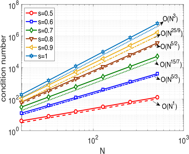
(a) ${\rm Cond}\sim N^{\alpha(2s-1)+1}$         

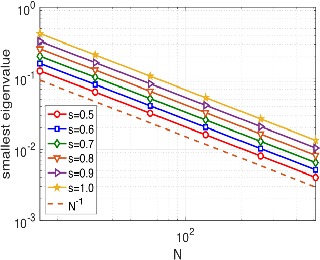
(b) $\lambda_{\min}\sim N^{-1}$         

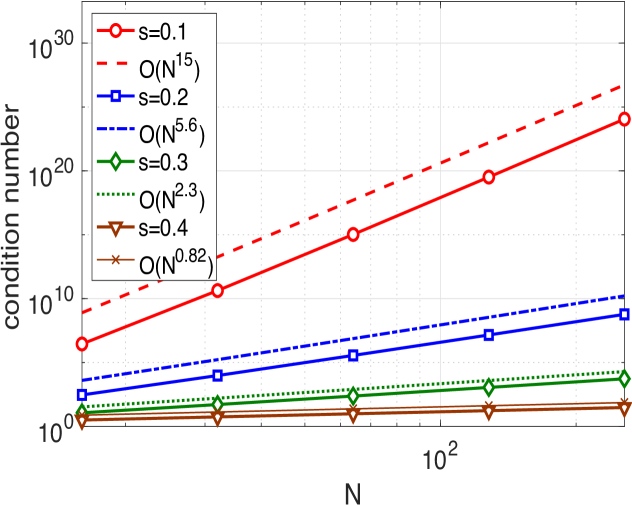
(c) ${\rm Cond}\sim N^{(\alpha-1)(2s-1)\mu(s)+2s}$     

Figure 1. Conditioning and the smallest eigenvalue of the stiffness matrix $\bm{S}$ with $\alpha=2/s.$ (a)-(b): various $s\in[1/2,1].$ (c): various $s\in(0,1/2)$.

3.3. Numerical results

It is known that the solution of the fractional Poisson problem (3) with a smooth source term $f(x)$ exhibits singularities near the boundary of $\Omega$ (cf. [6]). In particular, we find from [3] that

$$(-\Delta)^{s}((1-x^{2})^{s}_{+}P_{n}^{(s,s)}(x))=\frac{\Gamma(n+2s+1)}{n!}P_{n}^{(s,s)}(x),\quad x\in\Omega=(-1,1),\;\;s>0,$$

where $P_{n}^{(s,s)}(x)$ is the Jacobi polynomial of degree $n$, and $u_{+}(x)=\max\{u(x),0\}$. In the following computation, we take $f(x)=1$ in (3), and its exact solution is $u(x)=(1-x^{2})^{s}_{+}/{\Gamma(2s+1)}$. Following the same lines as in the proof of [1, Thm. 6.2.4], we can show that

$$\max_{|x|\in\bar{\Omega}}\big{|}(u-I_{h}u)(x)\big{|}\leq cN^{-\min\{2,\alpha s\}},$$ (26)

where $I_{h}u$ is the piecewise linear FEM interpolation of $u$ on the mesh (19) with $\alpha=\beta>1.$ As a result, the optimal order can be achieved when $\alpha=2/s.$ With the explicit form of $\bm{S}$ in Theorem 1 and the aid of the Matlab toolbox [8] (for some extreme situations, e.g., $s=0.1$ with ${\rm Cond}(\bm{S})\sim N^{15},$ see Figure 1(c)), we demonstrate that the same accuracy can be attained when the FEM solution $u_{h}$ of (5) is in place of $I_{h}u$ in (26). We observe from the numerical error plots in Figure 2 that the convergence rate of the FEM solver agrees well with the theoretical prediction.

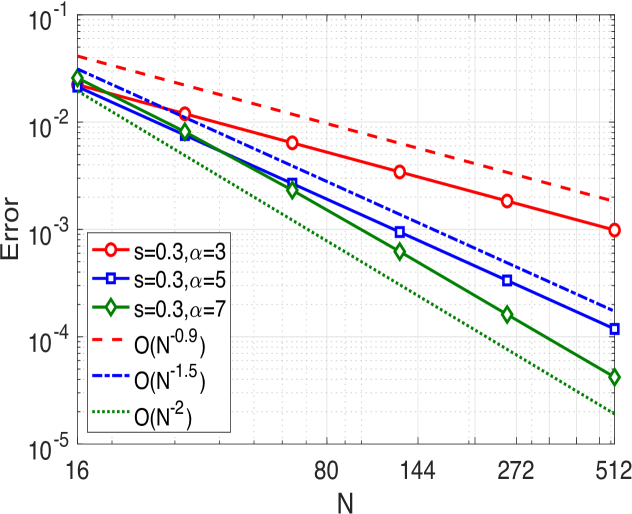
(a) Conv $\sim N^{-\min\{2,\alpha s\}}$      

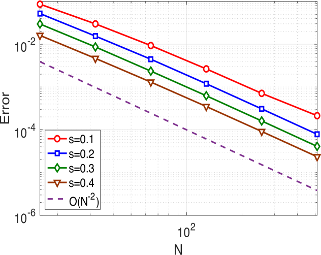
(b) Conv $\sim N^{-2},\alpha=2/s$

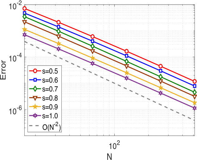
(c) Conv $\sim N^{-2},\alpha=2/s$

Figure 2. Convergence order of the FEM solver on graded meshes. (a): $s=0.3$ and different $\alpha$. (b): various $s\in(0,1/2)$ and $\alpha=2/s$. (c): various $s\in[1/2,1]$ and $\alpha=2/s$.

In Figure 2, we present the maximum errors of our method against $N$ (where $N$ denote the number of elements, see (LABEL:xmesh)) with various $s$ for two different meshes. We observe from Figure 2 (a) that the convergence rate of graded mesh are $O(N^{-\min(rs,2)})$, for which we take $s=0.3$ and various $r$. Meanwhile, Figure 2 (b) indicate that the numerical errors can achieve the second order convergence rate by choosing $r=2/s$, which is consistent with the result in [1, Theorem 6.2.5]. Moreover, Figure 2 (c) show that the numerical errors decay exponentially as $N$ increases for geometric mesh, where we fixed $q=0.96$.

We further show the smallest eigenvalue, largest eigenvalue, and condition number of the stiffness matrix $\bm{S}$ for two different meshes. For graded mesh, we observe from Figure LABEL:eigsmall (a)-(b) that the smallest eigenvalue of is behavior like $O(N^{-0.4r})$, which implies the decay rate of the smallest eigenvalue only depends on $r$. Figure LABEL:eigsmall (d) indicate that the decay rate of the largest eigenvalue only depends on $s$, and Figure LABEL:eigsmall (e) show that the largest eigenvalue for graded mesh with $s=0.3,0.7,1$ are $O(N^{-0.4}),O(N^{1.1}),O(N^{3})$, respectively. For geometric mesh, the smallest eigenvalue is decay exponentially for $s<0.5$, the largest eigenvalue is increased exponentially for $s>0.5$, and the smallest and largest eigenvalues remain a constant for the other case (see Figure LABEL:eigsmall (c) and (f)). Therefore, we can see from Figure LABEL:cond (a)-(b) that the condition number of stiffness matrix behavior like $O(N^{rs+\epsilon})$, where $\epsilon$ is a small real number. We also observe from Figure LABEL:cond (c) that the condition number of stiffness matrix with geometric mesh grows exponentially as $N$ increases.

4. Concluding remarks and discussions

Different from the implementation of FEM in the physical space, we computed the stiffness matrix of piecewise linear FEM for the IFL in the frequency space, and derived the exact form of the entries. In fact, this approach can be extended to two-dimensional rectangular elements, but it is much more involved, which we shall report in a separate work. Here, we studied the graded mesh, and numerically demonstrated how the condition number of the stiffness matrix grew with the parameters. One message is that computation with multiple precision is necessary, in order to reduce the round-off errors in evaluating the entries of the fractional stiffness matrix and battling its large condition number. In this study, we only considered the fractional order $s\in(0,1],$ but the formulas in Theorem 1 are valid for $s<3/2,$ which we leave for future investigation.

References

• [1] H. Brunner, Collocation Methods for Volterra Integral and Related Functional Differential Equations, vol. 15, Cambridge University Press, Cambridge, 2004.
• [2] M. D’Elia and M. Gunzburger, The fractional Laplacian operator on bounded domains as a special case of the nonlocal diffusion operator, Comput. Math. Appl., 66 (2013), pp. 1245–1260.
• [3] B. Dyda, A. Kuznetsov, and M. Kwaśnicki, Fractional Laplace operator and Meijer G-function, Constr. Approx., 45 (2017), pp. 427–448.
• [4] I. Fried, Condition of finite element matrices generated from nonuniform meshes, AIAA Journal, 10 (1972), pp. 219–221.
• [5] I. S. Gradshteyn and I. M. Ryzhik, Table of Integrals, Series, and Products, Elsevier/Academic Press, Amsterdam, 8th ed., 2015.
• [6] G. Grubb, Fractional Laplacians on domains, a development of Hörmander’s theory of $\mu$-transmission pseudodifferential operators, Adv. Math., 268 (2015), pp. 478–528.
• [7] H. Liu, C. Sheng, L.-L. Wang, and H. Yuan, On diagonal dominance of FEM stiffness matrix of fractional Laplacian and maximum principle preserving schemes for fractional Allen-Cahn equation, arXiv:2007.08183, (2020).
• [8] Multiprecision Computing Toolbox. Advanpix, Tokyo. http://www.advanpix.com.
• [9] L. Wang and J. Shen, Error analysis for mapped Jacobi spectral methods, J. Sci. Comput., 24 (2005), pp. 183–218.