Draft \SetWatermarkScale1
Coverage and Energy Analysis of Mobile Sensor Nodes in
Obstructed Noisy Indoor Environment: A Voronoi-Approach
Abstract
The rapid deployment of wireless sensor network (WSN) poses the challenge of finding optimal locations for the network nodes, especially so in (i) unknown and (ii) obstacle-rich environments. This paper addresses this challenge with BISON (Bio-Inspired Self-Organizing Network), a variant of the Voronoi algorithm. In line with the scenario challenges, BISON nodes are restricted to (i) locally sensed as well as (ii) noisy information on the basis of which they move, avoid obstacles and connect with neighboring nodes. Performance is measured as (i) the percentage of area covered, (ii) the total distance traveled by the nodes, (iii) the cumulative energy consumption and (iv) the uniformity of nodes’ distribution. Obstacle constellations and noise levels are studied systematically and a collision-free recovery strategy for failing nodes is proposed. Results obtained from extensive simulations show the algorithm outperforming previously reported approaches in both, convergence speed, as well as deployment cost.
1 Introduction
Wireless Sensor Networks (WSN) are used pervasively in the context of e.g., the monitoring of physiological and environmental parameters, for object tracking and surveillance or in smart homes [1, 2, 3]. WSNs are commonly optimized with regard to connectivity, coverage, localization, lifetime and dynamic adaptation [1, 4, 5, 6].
Since the surrounding environment affects the localization of sensor nodes and impedes the data transfer between nodes [4], the robustness of WSN against noise-driven disruptions is a relevant performance measure. Moreover, WSNs are often supported by low power devices, making energy efficiency a factor that possibly affects e.g., the lifetime of the network or the complexity of the algorithms.
The efficient deployment of sensor nodes (fast and cheap while delivering maximum service) is a main issue [7, 8, 9], especially in scenarios where this has to happen with limited or no prior knowledge about the target environment.
To facilitate rapid deployment, a common approach is to move nodes into an environment continuously (on-the-fly) and based on what they can sense in real-time [10, 11].
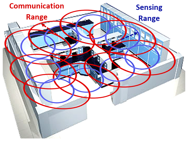
In this paper, we propose a Voronoi-based algorithm called BISON, (for Bio-Inspired Self-Organizing Network), for providing nearly optimum solution to self-deployment and localization of a WSN in an unknown bounded region of interest with obstructions such as in Fig1, in the presence of noise distortion.
BISON evolves the positioning of the sensor nodes inside an area, making use of their distribution to maximize the coverage and maintain the connectivity through controllable injection conditions. To facilitate energy conservation we compute the nodes’ next positions iteratively and based solely on local information (i.e., about a node’s neighbours within its sensing range) [12, 13]. BISON’s performance improves in the presence of various levels of Gaussian noise, which makes it useful for implementations.
In §2 we briefly discuss existing Voronoi-based algorithms for WSN and highlight the novelty in our self-organizing network (BISON) (introduced in §3). Our model and its implementation is provided in §4. In §5 we define our evaluation metrics for comparison of the proposed approach with representative competitive algorithms, the parametric performance analysis is discussed in §6.
2 Voronoi-based Algorithms for WSN
2.1 Inspiration and state of the art
Animal strategies of self-organization to reach a dynamic steady state distribution have inspired the application of such behaviors in mobile networks [11, 14, 15, 16]. A known benefit is the ability to operate with a minimal amount of information about the environment, yet to achieve near optimal solutions with low(er) computational demands. Whether they are considered a geometrical phenomenon [17], or a bio-inspired one [12, 18, 19], Voronoi tessellations are among such techniques. Fig. 2 offers a brief schematic review for Voronoi-based algorithms goals and techniques, for more details we refer to Fig. S1 of the Supporting Online Materials (SOM, hereafter). Territorial behaviour in animals such as for the male tilapia mossambica (a fish species) and how polygonal shapes of sufficient density are formed is discussed in [19]; an illustration is found in Fig. S2 in SOM.
By mimicking such behavior, sensor nodes in a WSN can generate Voronoi regions (convex polygons that together partition an area) based on local information and subsequently adjust their positions until the change per iteration falls below a system convergence condition. The boundaries of the polygon are generated by drawing the perpendicular bisector of each segment connecting the cell node with its neighbor nodes (for a pictorial representation of this cf. Fig. 7 on page 7 or Fig. S2 in SOM).
This process tends to achieve uniform distribution during the self-organizing process, motivating WSN researchers to analyze and identify the coverage holes after the initial distribution of sensors. Voronoi algorithms have been used to enhance network-coverage and -connectivity, either stand-alone [20, 21, 22] or in tandem with bio-inspired algorithms [23, 24, 25, 26, 27].
For known areas and a fixed number of homogeneous sensor nodes, Wang et al. [28, 29, 30] developed three different coverage-optimizing algorithms which re-allocate the nodes to positions covering most of the Voronoi vertices/edges within the sensors’ sensing ranges. Apart from the vertices, there is a substantial interest towards approaching the centroid (center of mass of a Voronoi cell) during sensors’ re-allocation, known to provide better uniform node-distribution while requiring less movement [20, 21, 22, 31]. An example with the use of a Voronoi centroid is discussed by Zou et al. [32, 33, 34, 35] who introduced Node Spreading Voronoi Algorithm (NSVA) to self-deploy fixed number of nodes in an unknown obstacle-free area.
Voronoi diagrams are also involved in WSN deployment of heterogeneous sensors, whether combined with Laguerre geometry to partition the regions between adjacent sensors, or adding weights on each sensor node based on its sensing range to create multiplicatively-weighted Voronoi diagrams [36, 37, 38, 39, 40]. Additionally, Voronoi diagrams are involved in the scheduling mechanisms of WSN [22], and are considered in security algorithms, providing robustness against malicious attacks that might affect the nodes identities during the deployment process [41].
2.2 Novelty of BISON
Previous discussions of Voronoi-based algorithms considered a random distribution of sensor nodes, with most algorithms relying on prior knowledge about the (often obstacle-free) environment and node locations while assuming a guaranteed connectivity among the sensor nodes. Relying on first scanning the entire environment to determine obstacle location before distributing nodes is putting a strain network resources such as time and energy [42, 43].
In contrast, our approach evolves the location of homogeneous sensor nodes in unfamiliar and obstructed noisy environments. This happens iteratively, allowing the nodes to investigate their injection process to direct themselves based on methodological conditions to achieve maximum coverage and to maintain connectivity in the network, without a priory assumption. In BISON, each nodes scans only its local environment to identify nearby obstacles, generates or updates its own Voronoi region (accounting for obstacles) and then directs itself toward its new Voronoi centroid.
In addition, the negative impact of communication noise on the distribution of nodes is addressed in the literature either by using anchor nodes of known locations to predict the location of all other nodes (using fuzzy logic methods), or by adding a (random) uncertainty value to the measured distances between the nodes and their neighbors. In our work we simulated realistic communication noise (Gaussian) and embedded this in the information about nodes’ locations (used extensively in the deployment process).
Finally, we will show (a) that involving Voronoi-based centroidal WSN node deployment in BISON is efficient in the removal of dead / tired nodes with least distance traveled among the nodes, as well as (b) how underlying kinematics of WSN nodes are affected by environmental noise that lead to improvements in the network coverage. The latter we demonstrate in our noise coherence analysis.
2.3 Contribution of this article
Our work is guided by three main goals:
-
1.
Propose an approach that can handle the inclusion of obstacles and is capable of examining their effect.
-
2.
Examine / evaluate the performance of the proposed approach when subjected to noise.
-
3.
Ensure resilience against uncontrollable loss of WSN nodes and facilitate controlled node removal / exiting of low energy nodes by providing individual exit paths.
The main contributions to, and improvements over, the state of the art are that we evolve sensor nodes’ locations without (1a) a priori fixing their number or (1b) relying on special injection conditions to ensure network coverage and connectivity; that the approach is designed for unknown environments (2a) with obstacles but (2b) without a prior demand on a continuous connected network; (3) that the system is subjected to communication noise. We also (4) show that the swarm coherence method is an effective tool.
3 The BISON Algorithm
The proposed algorithm evolves network nodes inside an environment, following certain methodological conditions that aim for optimum coverage while maintaining connectivity without a priory assumption. A centroid Voronoi tessellation mechanism is implemented for the deployment of nodes in an unknown noisy environment with obstacles. The number of nodes involved in the deployment process is unknown (but finite) and dynamically determined by gradual and conflict-free absorption. The node injection conditions are designed to ensure full coverage and connectivity. Node movement is achieved through self-organization, with the new allocation of nodes guided by the nodes’ desire to move towards the respective center of their Voronoi cell; cf. Fig. S3 in SOM for a flowchart of the BISON algorithm.
3.1 Voronoi regions in obstacle free environments
Unlike in prior art, the Voronoi regions in BISON are are not only characterized by the neighboring nodes, which might drop the connection in noisy environment or drop out altogether unexpectedly. Instead, the configuration is dependent on observations within a sensor’s sensing range; the Voronoi regions are the intersection between the neighboring bisectors, the obstacles, and the sensor’s sensing range.
For starters, any point inside the environment is assigned to the region of a specific node (cf. [18]):
| (1) |
Practically, the allocations defined by Equation 1 are formed continuously through local interaction: the nodes perpendicular bisectors are calculated using the Euclidean distance to neighbouring (i.e., within communication range) nodes. The more restricted BISON Voronoi regions are determined using the intersection between the perpendicular bisectors and the node’s sensing range ().
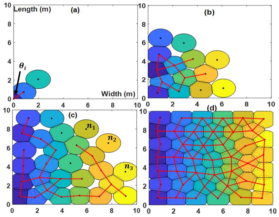
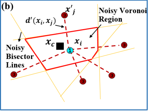
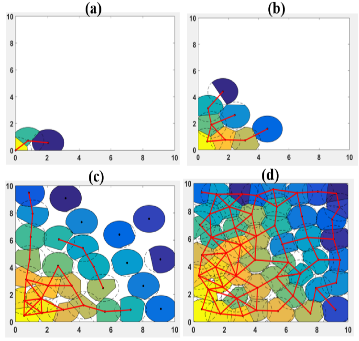
For nodes at the outer rim of the network (in Fig.3 (c): e.g., , and ) their Voronoi region is their sensing range: . These nodes are temporarily static (as they already are at their Voronoi centroid) and disconnected from the network. As additional nodes are injected, these outer nodes will be reached and pushed out further.
3.2 Node injection
With regard to additional nodes being added, this is conditional on either of the following two conditions:
-
1.
there are disconnected nodes, or (c1)
-
2.
there is unexplored space left. (c2)
To formalize this, we first impose the requirement of connectivity, i.e., that every node has at least one neighbouring node within its communication range :
If anode is violating this then condition (c1) is met and an additional node is injected. Practically, this is implemented by maintaining an account of the number of injected nodes and comparing this to the nodes currently relaying information in the network (a known / knowable property).
Secondly, we require that there is at least one node within sensing range of the point of injection:
Assuming that the injection point is at the border of the area, the diffusion of the nodes across the area will cause the node closest to the injection point to drift away if there are uncovered locations anywhere in the area. Therefore, if the above is violated then we can conclude that there are uncovered areas (amongst them the injection point), which violates condition (c2) and causes another node to be injected. Jointly, these two conditions ensure coverage and connectivity; furthermore, in any finite area these conditions can be realized with a finite number of nodes.
3.3 Node movement
Nodes continuously move towards their Voronoi centroids (the center of mass of each node’s Voronoi region), thereby ensuring gradual and directed movement towards complete area coverage [44]. This process requires first to find the center of mass of each node’s Voronoi region . Any region is a polygon with vertex coordinates , and we calculate its area and center of gravity using measure (with and to come full circle) [45]:
Area is the area of polygon . Once we have this, the x-/y-coordinates of its center of gravity can be found as follows:
The distance to its center of gravity, i.e., the difference between the Voronoi centroid () and the node’s actual location () - together with application specific parameter can be used as termination condition. If the aggregated movement of the node over a number of steps does not exceed then the algorithm terminates. This is measured over all nodes (cf. Alg. 1, below) or, for true decentralization, for each node individually.
4 Modelling and implementation
In this section we provide additional information regarding the model used for our implementation and approach. In addition to the basic modelling choices made we discuss how obstacles and noise were included in the system and how real-world aspects such as node-failure were modelled.
4.1 Preliminaries and basic modelling choices
The following basic modelling choices were made:
-
1.
All nodes are homogeneous with equal sensing-, communication-, computation-, and mobility-abilities.
-
2.
To make the simulations more realistic, the deployment of the sensor nodes happens iteratively, one at a time and from a fixed entry point at the edge (here: ).
-
3.
Node-injection is triggered by conditions (cf. §3.2) that verifiable at the entry point; the node’s individual entry angle () is random, between and .
- 4.
- 5.
-
6.
The threshold for our termination criteria was set to one hundredths of the sensing range of a cell:
4.2 Introducing obstacles
4.2.1 Motivation
Virtually all WSNs are deployed in environments with obstacles that obstruct the wireless connection in one way or another. This means that environments such as the one depicted in Fig. 3 are over simplified.
To account for this we have included signal obstructions (i.e., obstacles) into our model. Figs. 4, 5 and 6 show different aspects of obstacles included in the environment.
4.2.2 Modelling
As mentioned in §4.1, we model the sensing range of a node to be circular (omni-directional, transmitting their signal ). Signals bounced back by an obstacle can be used to determine the location of the obstacle [50]. In our simulation, the calculations required to infer the location of an obstacle is omitted, the relevant information is simply provided when calculating the Voronoi region (which is generated based on the detected obstacle boundaries, the node’s sensing range, and the neighboring bisectors).
We considered three types of obstacles in environments:
-
1.
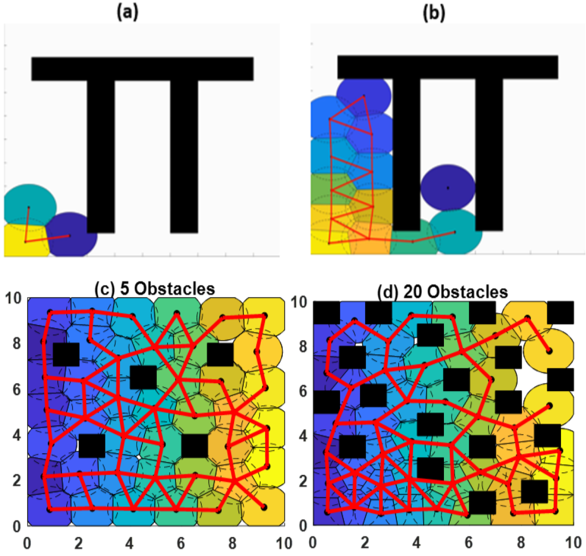
small (1 measurement unit), free-standing obstacles that correspond to pillars or vegetation, cf. Fig. 4 (c) and (d). For the evaluation of the algorithm we simulated environments containing 5 (c) to 20 (d) obstacles.
-
2.
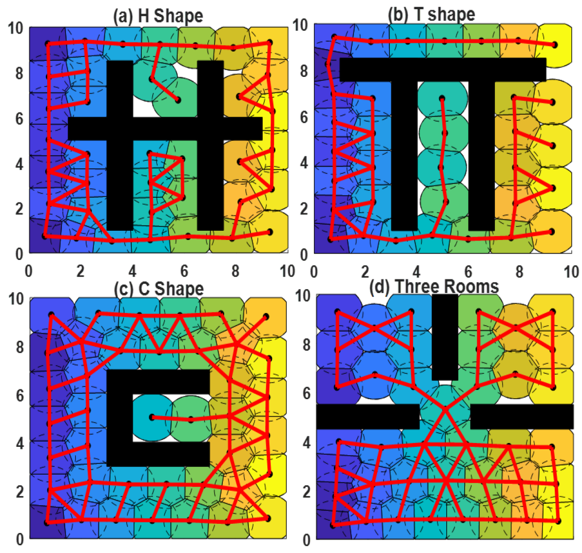
large, elongated rectangular obstacles representing e.g., walls. 4 different configurations were used, cf. Fig. 5.
-
3.
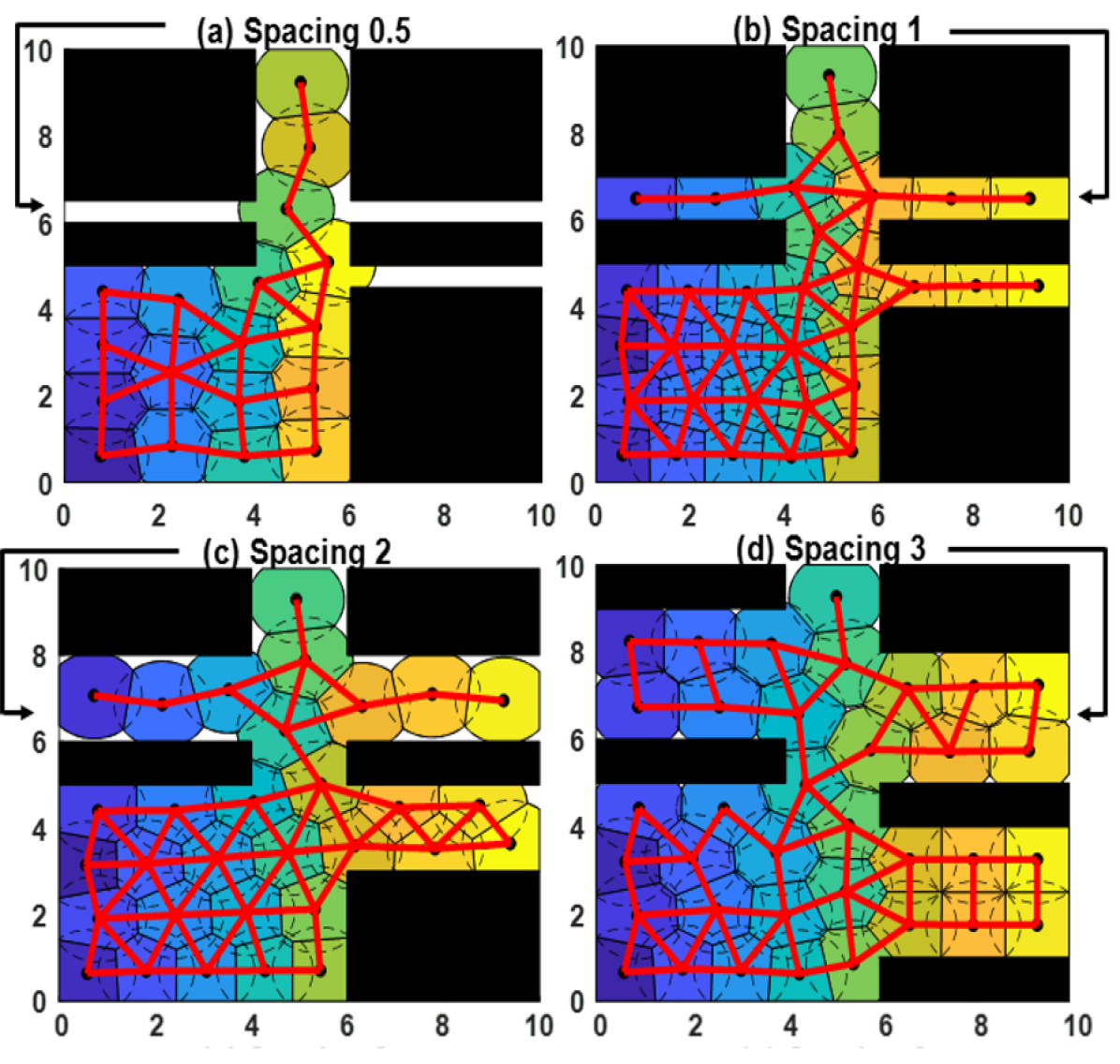
elongated cavities as found e.g., between factory equipment, cf. Fig. 6. BISON was tested over a number of variations of this environment, with the distance between obstacles ranging from 0.5 to 3 measurement units (corresponding to to of ).
These 4 contain all challenges we identified when looking at floor plans.
The goal was to consider small and large obstacles as well as to explore the ability to deploy WSN into areas with relatively small cavities. The specific instances within each type (cf. Figs. 4, 5 and 6) were, however, relatively freely chosen and are therefore not guaranteed to exhaustively represent all possibly occurring environments.
4.2.3 Implementation
The formulae for the calculation of the Voronoi centroid, presented in §3.3, are applicable to all solid polygons. However, while unlikely to happen in our simulation, the calculation for polygons with “holes” (pillars) requires extra steps: we have to first decompose the region into smaller, solid regions. Using the calculation for an Area from §3.3, the Voronoi centroid () of a non-convex polygon was then calculated using the centroids of its sub-polygons (), , () together with the respective areas as follows [44]:
4.3 Adding noise
4.3.1 Motivation
As suggested by the name, nodes in a WSN communicates use wireless communication. This is unshielded and naturally incurs distortion and noise from the physical environment. In the context of this article, we only concern ourselves with the impact of noise regarding the determination of the position of neighbouring nodes.
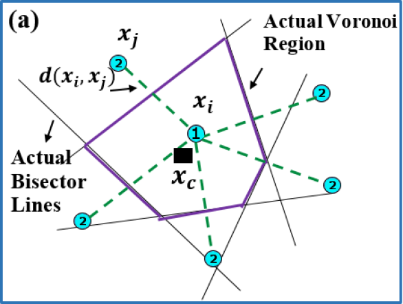
In BISON, nodes regularly check up on their neighbours and attempt to determines their distance to them. The accuracy of this process is affected by the noise in the sensed values and the resulting uncertainty will in turn impact the determination of the bisector lines, which are used to calculate the node’s Voronoi region.
To visualize this, Fig. 7 (left) shows the actual locations of nodes neighbouring 1, labelled 2, as well as (right) the erroneous perceived positions, labelled 3. Using node (correct location) / (erroneous location) as an example we illustrate the impact noisy sensing can have on the calculation of the bisecting lines and subsequently on the resulting Voronoi region. Depending on the level of noise, the latter can thus differ significantly which can lead to a significant loss of overall coverage (cf. Fig. 8).
In contrast to e.g., [34], where randomization was used, we wanted to use a specific noise function. This (a) allows us to investigate the performance of BISON under various degrees of noise distortion (see §4.3.3) as well as (b) facilitates subjecting the system to other, environment specific, noise functions (potential future work).
4.3.2 Modelling
In communication channels, additive white Gaussian noise (AWGN) is used to describe the noise affecting the communication channel. Noise is added to the signal with uniform power across the transmission channel.
AWGN is the simplest model of Gaussian distribution with zero mean, modelled as statistical noise with a probability density function P(x) (normal distribution) as follows:
| (2) |
with and the mean and standard deviation of random variable , respectively. Increasing variance (given by with the noise power) has an increased (detrimental) effect on signal accuracy.
4.3.3 Implementation
The effect of is felt only within . I.e., visibility of neighbouring nodes is maintained but their derived locations may be subject to error. Three different noise-levels were considered in our simulations: (low), (medium) and (high).
4.3.4 Impact
Including signal distortion means that incorrect Voronoi centroids are being calculated by the nodes (cf. Fig. 7), causing them to move to a position other than the actual center of gravity, as defined by Equation 1. This in turn can cause incomplete coverage (cf. Fig. 8, (d)) as well as continued (and unnecessary) consumption of energy as nodes keep moving around their actual Voronoi centroid.
Furthermore, signal distortion can affect the usefulness of the termination condition we use (see next section).
4.3.5 Additional stop criterion
In noisy environments, and as nodes become increasingly scattered, signal distortions can cause nodes to keep moving back and forth which may result in them exceeding threshold (cf. §3.3), used in Alg. 1 as the first of two termination criteria. Because of this, a second criteria is devised as follows: using a pre-defined minimum network coverage area min and a constant cmax (set in our simulation to cmax), we stop the algorithm after exceeding min and when there was no increase in the coverage area for cmax consecutive iterations (while the network is fully connected); see Alg. 1.
4.4 Node-failure and self-organizing recovery
4.4.1 Motivation
Having considered real-world challenges in environments (such as obstacles and signal-noise), it would be strange to ignore practical issues of the sensor nodes themselves. Under realistic deployment conditions, a WSN is likely to face sudden / unexpected loss of nodes sooner or later. This may be due to a number of reasons, with the most common examples being device malfunction, resource (battery) depletion or outside influences.
4.4.2 Modelling
The modelling of node-failure is straight-forward, in our implementation we can simply remove a node from the WSN. That being said, we would like to distinguish three types of nodes: devices whose Voronoi region touches (1) only other Voronoi regions, (2) one wall or (3) two walls (in which case the node is in a corner).
4.4.3 Implementation
To enable node-failure handling, no additional implementation is required: losing a node means that some of the remaining nodes lose a neighbour. This means that their Voronoi regions (and thus centroids) change, wich causes them to move. This will happen until coverage is restored. Note that this might cause additional nodes to be injected (but that as well is functionality that is already implemented, cf. §3.2).
4.4.4 Additional considerations
With more complex systems and increasingly autonomous nodes in mind, we briefly touch on the subject of planned / intentional node-loss. This can e.g., be the case when an individual node is low on power and autonomously decides to return to the injection point to recharge. In that case an approach would be to let a node continue to provide coverage until its Voronoi region is entirely taken over by its neighbours. A practical issue would then be the path planning for the now redundant node, which is briefly discussed in §6.5.
5 Evaluation Metrics
In this section, we define the four major metrics used to evaluate the WSN created by BISION: the coverage achieved by the WSN, the combined distance travelled by the nodes to achieve this coverage, the energy consumed to do so and, finally, the uniformity of the node distribution.
5.1 Percentage Area Coverage (PAC)
5.1.1 Motivation
While we are aware of WSN-applications that operate under (sometimes extreme) resource scarcity, our algorithm was designed to achieve full coverage in scenarios of resource abundance, meaning that our concern is “covering the complete area” and not “how to cover as much as possible given a small number of nodes”. We will therefore use the area covered (in percentage of the environment) as a performance measure and to plot progress during the deployment phase of the WSN.
5.1.2 Modelling
5.2 Distance Traveled (ADT / CDT)
5.2.1 Motivation
The energy requirements for a successful deployment of WSN using BISION was an important parameter to consider. While we provide a separate measure for the actual energy consumed (cf. §5.4) we first want to evaluate performance de-coupled from the energy cost incurred by the operation of the network (i.e., without the cost generated by sensing and signal operations), and we did so by measuring the distance traveled by the nodes.
We measure the distance traveled by the nodes in two ways: we fist consider the simple value of how much, given a current positions of the nodes, each node would have to move if it directly went to the current position in the deployment. This is called the average distance traveled (ADT). In addition, we capture the far more accurate value of the cumulative distance traveled in the network (CDT), i.e., the distance that was actually traveled, including the noise-induced bouncing back and forth between positions.
5.2.2 Modelling the average distance traveled (ADT)
We used the following equation [32, 34] to analyze the average distance traveled (ADT) by the sensor nodes:
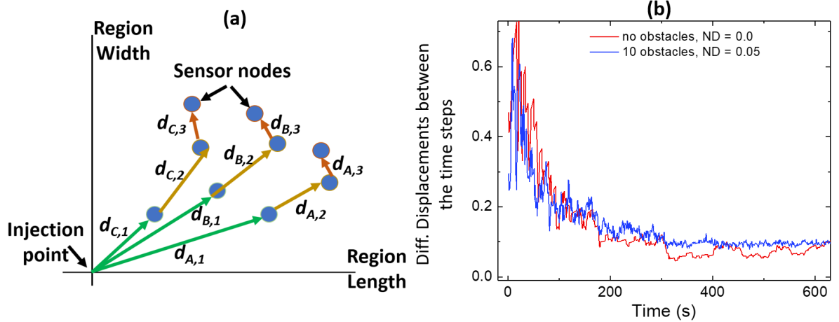
where n(t) is total number of nodes at time t, origin is the initial location / the injection point of node i (for us that is fixed to ). are the current x-/y-coordinates of node i. Note that unlike in the literature [32, 33], we do not require the number of nodes to be constant over time.
5.2.3 Modelling the cumulative distance traveled (CDT)
The cumulative distance traveled (CDT) is measured recursively over the iterations the network has undergone. At time the combined movement of all cells is zero, at any other time the CDT is the sum of all CDTs in preceding time-steps plus the movement since :
With the absolute Euclidean distance between the previous location of a node and its current one.
5.2.4 Implementation
CDT is implemented as a variable that is iteratively updated in Alg. 1: the value for the distance moved () is calculated as follows:
In Alg. 1, the value for ) are then stored in the variable ; the calculation of CDT is a question of aggregating these values (in the variable shift).
With regard to ADT, since all nodes enter at the same injection point ) this can be easily calculated:
5.3 Deployment behaviour over time (velocity)
5.3.1 Motivation
When evaluating the performance of BISON we are not just interested in the distances traveled by nodes but also in their collective behaviour. In line with [51] we will use the average node-velocity to characterize node behaviour during the deployment of the WSN.
In our simulation, individual node velocity is determined by the calculation of the Voronoi centroid combined with the node’s inference of its location (i.e., the to and from of the node’s movement). The way we determine movement defines the overall collective deployment behaviour but considering the distance (as we do with ADT and CDT) only gives us insight into the performance of the entire system and does not tell us anything about the performance of the nodes in the context of the behaviour of the other nodes.
5.3.2 Modelling node–diffusion and –drift
In line with [51] we avoid using a theoretical complex model / equation to determine node-velocity; instead we use empirical data (generated by our simulations) to estimate the diffusion () and the drift () coefficients of this equation. The former will capture the mean rate of change of average node velocity, while the latter quantifies the evolution thereof.
The coefficients for diffusion () and drift () are defined as follows [51]:
| (3) |
| (4) |
with
where is the average velocity of all the available nodes at time , is the diffusion coefficient, the drift coefficient and the chosen time step value.
5.4 Energy cost incurred for deployment
5.4.1 Motivation
Nodes in wireless sensor networks almost always operate with a limited energy budget. Since the energy consumption of individual nodes as well as that of the entire WSN are of paramount interest to practitioners in the field, this has to be considered in our evaluation.
Generally speaking, energy efficiency is commonly measured over the lifetime of a network [52, 53]:
| (5) |
where is the total energy that sensor nodes are provided with, is the cost incurred by moving the nodes and is the cost incurred by operating the sensing equipment. To account for more complex implementations we can add , sub-summing any additional power requirements.
5.4.2 Modelling
In the context of this article, we are only concerned with the energy cost incurred by the movement of a node . In the literature [49, 54], was modeled (based on kinetic energy) as follows:
| (6) |
where m is the mass of the sensor node, is the time step of node i, , is the distance moved during time step , and is the corresponding velocity of the node at . Under the reasonable simplifying assumption that the work-energy theorem applies, this expression could be reworked into:
We will use mass-normalized energy, , to further focus on kinetic aspect of the problem.
5.5 Uniformity of the coverage
5.5.1 Motivation
As the area in a circle (sphere) increases non-linearly with the radius, so does the signal strength of a broadcast diminish with distance to the emitting device. Providing a certain signal over a distance does therefore incur an energy cost that is also non-linear in the distance to the source. Therefore, and in all generality, if complete coverage can be achieved by all nodes in a network operating at the same coverage radius then this is guaranteed to be (as far as signal cost is concerned) the best possible set-up.
For us this translates to the goal to reduce coverage overlap as much as possible. Since we are operating in an obstacle-rich environment we do not compare the coverage radii but instead the areas inside the Voronoi regions.
5.5.2 Modelling
Following [34], we capture the extent to which Voronoi regions covering an area are uniformly distributed over the nodes in a network by measuring the similarities between the generated polygon regions :
| (7) |
where is the area of Voronoi cell i and is the total number of nodes in the network. The smaller the value of the better the system is towards uniform distribution.
6 Results and Discussion
We evaluate the performance of BISON over time and under increasing noise-levels. We focus on two criteria: (1) the movement required to continuously grow the network until the termination criteria halt the algorithm and (2) the growth of coverage during deployment. We furthermore investigate the resilience of the network against node loss and provide a comparison to another approach for some insight into the convergence properties of the approach.
Overview
In §6.1 we first provide an overview over the implementation choices taken and sum up the various parameter settings discussed earlier in this article. We then report on three investigations into the performance of BISON: (1) in §6.2 we evaluate the algorithm with regard to the movement of the nodes in the different environment types we considered. There, we also present the results of comparing BISON to the NSVA algorithm with regard to performance and convergence. (2) We then (§6.3) discuss the coverage achieved by a WSN deployed through BISON. (3) Finally, in §6.4 we present our findings and considerations with regard to real-world aspects of swarming and node failure.
6.1 Materials and methods
The BISON algorithm (provided as Alg. 1) was implemented using MATLAB version R2017b. As mentioned, there are a number of control parameters and settings. Unless otherwise stated the following values were used in simulations for data collection and performance evaluation:
-
•
sensing range: (intended interpretation: one meter); communication range: .
-
•
simulated environment: .
-
•
inject node angle : random between and .
-
•
injection point (aka origin): (0,0).
- •
The following values were recorded during simulations:
- •
- •
6.2 Performance evaluation: movement
6.2.1 Movement in obstacle-free environments
To establish a baseline, BISON was used to deploy a WSN into an obstacle-free environment while the nodes were subjected to various levels of noise. Both, the average- (ADT) as well as the cumulative- distance traveled (CDT) by the nodes in the WSN were recorded and are plotted in Fig. 9.
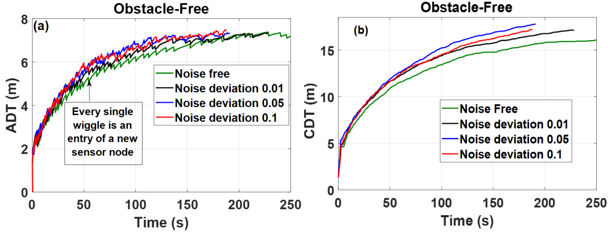
We would expect that the performance suffers as noise-levels increase. Indeed, at least with regard to the distances traveled this is initially the case for both ADT and CDT. However, upon closer inspection we see that for both measures the highest noise-level actually outperforms the second most severe noise-level: for the network requires less movement or time than it does for .
Furthermore, for both measures, the time required to reach the stop condition consistently decreases as the noise-level increases. This implies that noise can have a beneficial impact on collective performance. These results are consistent with the literature (cf. [34] on the NSVA algorithm in noisy environments); §6.4 is dedicated to exploring this, counter-intuitive result in more detail.
The CDT turns out to be roughly twice the ADT. As we will continue to compare these two measures it seems important to point out what exactly they represent again: both report an average value, but ADT uses the as-the-crow-flies distance while CDT uses the actual distance traveled. Thus, the factor by which CDT exceeds ADT is an indicator for the detours taken by the nodes to reach a position.
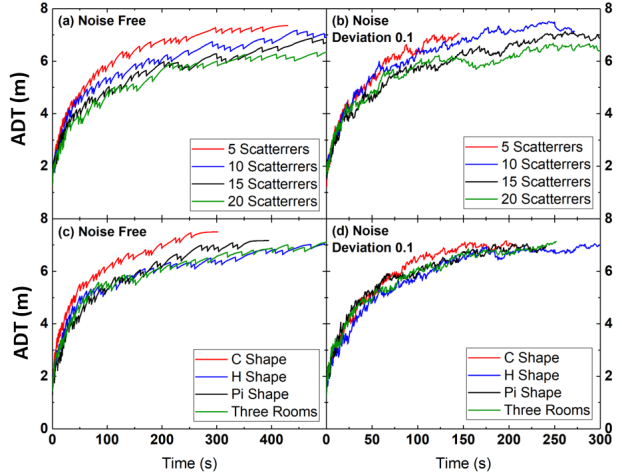
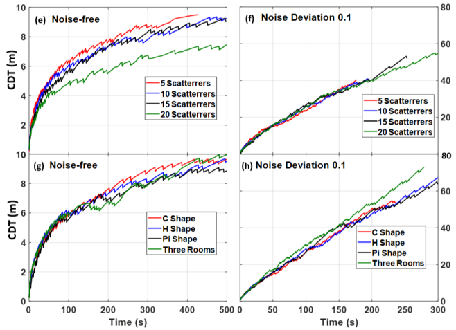
6.2.2 Movement in obstacle-rich environments
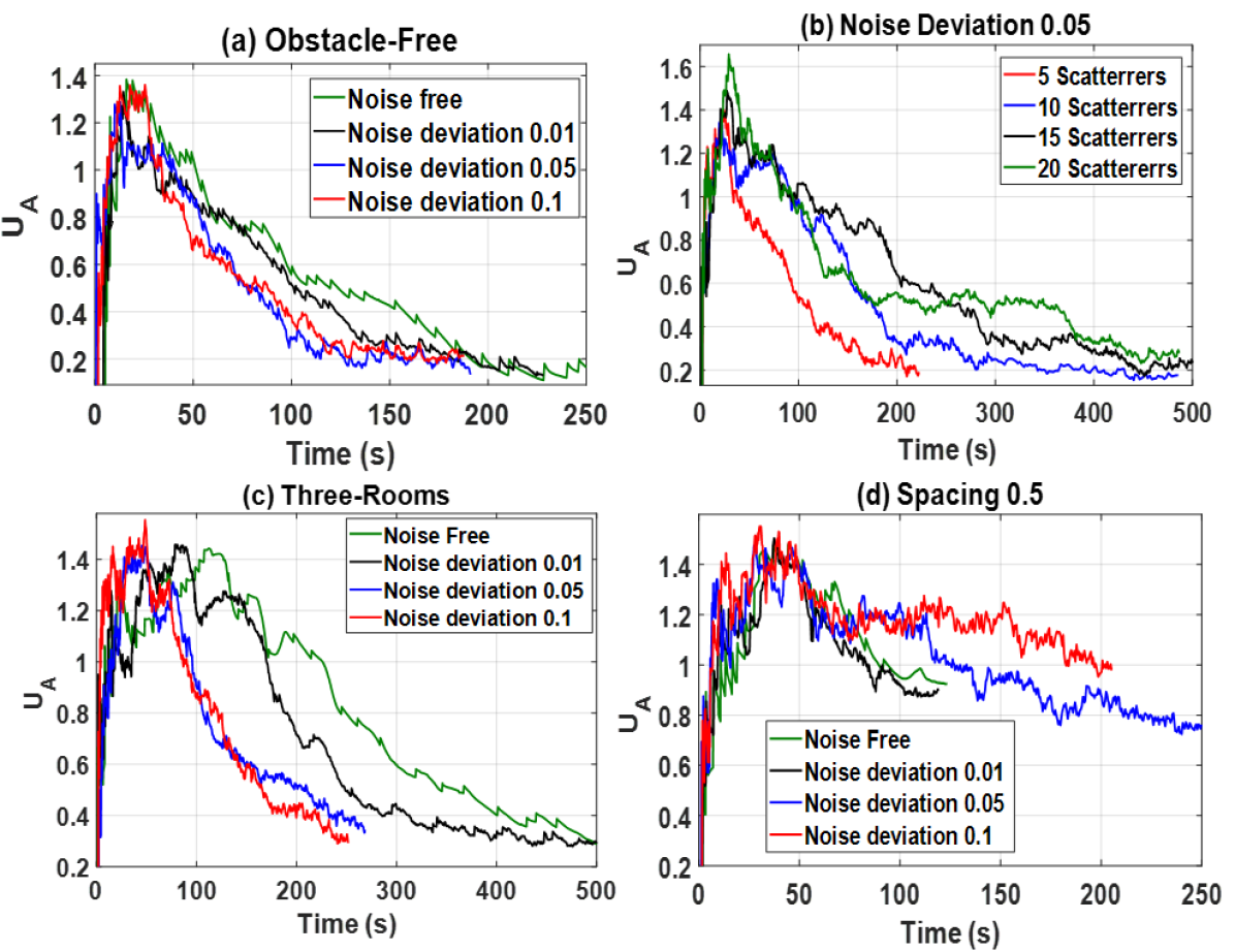
The positive effect of high () noise-levels - noticed in the previous section - is also consistently found in the results presented in this section. To enhance readability of Fig. 10, we only report on the outcomes for and “no noise at all”; the interested reader is referred to Figs. S4 and S5 in SOM for the other results, omitted here.
For obstacle-rich environments we report ADT and CDT separately again (cf. Fig. 10). We compare performance under lowest and highest noise level and for environments with signal scattereres (i.e., pillars) or walls.
The impact of noise
The first thing that we notice when comparing the results plotted in Fig. 10 is that for ADT and CDT as well as for both types of environments, the algorithms achieves coverage faster in the presence of noise.
Walled / scattered environments
Increasing the number of signal scattering objects in the environment reduces the distance traveled by the nodes, especially for ADT.
While increasing the noise-level actually improve collective performance (cf. §6.4) the reduced distance here can be - at least partly - explained by the fact that there is effectively less of the environment to cover as an increasing percentage thereof is filled by the pillars (cf. Fig. 4). However, for the 4 walled experiments this explanation does not hold: the scenarios C-shaped and 3 rooms have significantly less space taken up by their respective walls than the other two environments (cf. Fig. 5), yet their ADT differs greatly. This is not unexpected because, especially in case of 3 rooms, there is a bottleneck for the nodes to pass through. This is supported by the corresponding CDT where this scenario requires the largest cumulative distance traveled.
Different variations on environment types
The performance difference for different cases of an environment type was consistent across experiments, indicating that some environments are inherently more difficult to solve than others. An theoretical study of which scenario aspects this depends on is outside the scope of this paper.
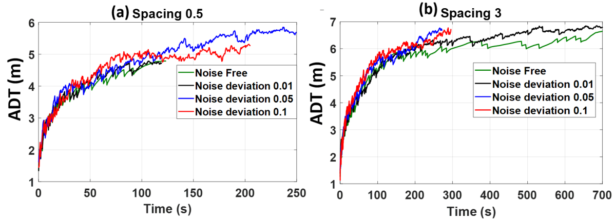
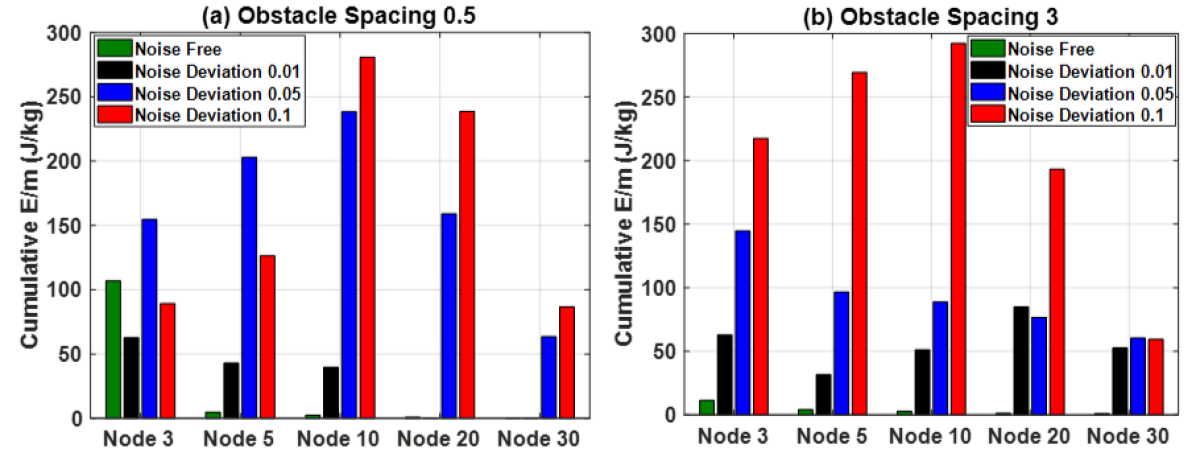
6.2.3 Movement in environments with crevices
First of all we refer back to Fig. 6, plot (a), to remind the reader that in the most restrictive scenarios (those where the spaces are merely a fourth of the nodes’ sensing range) the network simply fails to extend into these crevices. This obviously results in sub-optimal coverage but also means that less nodes are needed. Note that for all the tested scenarios (including the empty one), this was the only one where no noise, or low noise-levels outperformed higher noise-levels (cf. the plots in Figs. 9, 10 and 11). Avoiding the openings altogether does, however, impact the performance because the nodes facing these openings should be subjected to small incentives to move towards the openings (or into them) as their Voronoi regions are not restricted in that direction.
We report only on two of the 4 scenarios here; additional results, including results for all simulated scenarios and noise-levels are provided in S6 in SOM.
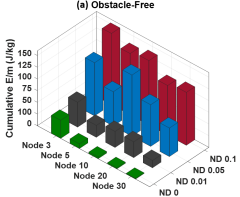
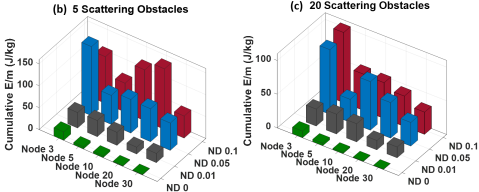
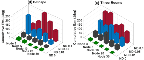
6.2.4 Cost incurred through node movement
Looking back at the plotted CDT values in Fig. 10, we clearly see that while the addition of noise consistently resulted in improved performance time it did so at a significant cost through increase in movement, as evident from Fig. 12.
When comparing the individual node movement with the resulting energy cost (cf. Figs. 9 and 12 for obstacle free– and Figs. 10 and 12 for obstacle-rich – environments; cf. Figs. 11 and 13 for environments with small spaces) we consistently see the trade-off. While the plots provided (reporting on the energy expenditures of some of the nodes) suffice to show that it is the environment and not the order of injection that determines the final energy cost, the full set of results / additional energy representation for obstacle-rich environments and cavities are provided on the SOM.
6.2.5 Convergence properties of BISON
We find no evidence that the modifications we introduced fundamentally alter the arguments (presented elsewhere in the literature [59] in favor of convergence of Voronoi algorithms. Nevertheless, we conducted a numerical experiment to compare performances of BISON (cf. Fig. 14).
Benchmarking of results
We compared node movement before and after coverage was achieved. Perhaps unsurprisingly, we see a rapid rise of the differential displacement as a function of time. After a maximum is reached, the motion of sensor nodes in the system rapidly decreases (cf. Fig. 14(b)). The maximum occurs close to the instant in time where a derivative of the PAC and ADT curves occur.
We furthermore compared BISON to closest related algorithm in the literature: the NSVA algorithm [32, 33]. The choice for NSVA was made due to its similarity in terms of the assumptions made, parameters used, as well as simulation time steps. In addition, it was important to use to compare to an approach that generates the Voronoi regions based on local information about the environment from the node’s sensing range, where other related algorithms (e.g., [20, 21, 28, 30, 31, 36, 37]) use global information or apply to heterogeneous nodes, which require different forms of Voronoi regions altogether. Finally, since the metrics used are, in fact, proposed in [32, 33, 34], the NSVA algorithm is the most obvious candidate for a comparative evaluation.
| Quantity | NSVA | BISON |
|---|---|---|
| Area () | ||
| () | 16 | 16 |
| () | 16 | |
| Number of nodes () | 40 | 16 |
| Time () | 150s | 20s |
| PAC (%) | 93.4% | 99.3% |
| ADT () | 74 | 85 |
Table I above provides a quick overview over the performance of both algorithms in an obstacle-free environment with no noise effect. The results of our comparative evaluation over time are plotted in Fig. 15: the left panel compares the algorithms on the basis of PAC while the right shows the respective ADT. Both inserts plot the difference between BISON and NSVA for the first 30 seconds of the simulation. BISON clearly outperforms NSVA.
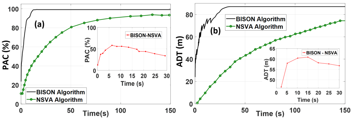
The performance is compared with BISON algorithm under the same parameters specified in Table I. It can be noticed that NSVA algorithm required 40 nodes and 150 to achieve 93.4% of area coverage, while BISON algorithm required one fifth of that time (terminating after 30) with 16 nodes to achieve 99% of area coverage. The improved speed can partly be attributed to the wider communication range , but this does not explain why BISON can operate with a significant smaller number of nodes.
To be fair, the final coverage is far more indicative of the superiority of BISON than the progress over time. The reason for this is that NSVA injects a fixed number of nodes inside the environment [32, 33] (here: 40) at start time while BISON injects its node as needed over time. Due to this, the plotted ADT in Fig. 15, right, has to be much better for BISON as most nodes in NSVA cannot move initially. However, BISON achieves a better coverage faster (cf. Fig. 15, left), and does so using significantly fewer nodes. In addition, lower energy consumption suggests a longer lifetime of the BISON network.
The observed difference between BISON and NSVA, shown in Fig. 15, inserts (a), (b), is only quantitatively different for the various environments and noise levels.
6.3 Performance evaluation: coverage
We evaluate performance using percentage area coverage (PAC), introduced in §5.1.2. Analogous to the results for movement (and thus energy cost) we find that increasing noise-levels have a significant effect on the performance: as before, the time required to achieve coverage decreases as noise-levels increase (cf. insert in Fig. 16). This comes at the cost of (significantly) increased energy consumption.
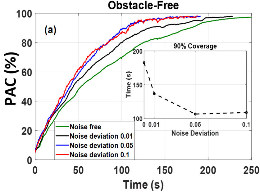
6.3.1 Coverage in obstacle-free environments
In obstacle free environments nodes can freely diffuse into the environment, obstructed only by the walls surrounding the scenario. With increasing noise-levels, however, the node’s Voronoi regions incur increasing error which directly translates to spotty coverage, affecting the PAC. As shown in Fig. 16, the ultimate outcome is nearly the same (differing by less than 1% in the achieved final coverage, which was 99% for noise-free environments and 98% for environments with high noise). However, when looking at the graphs plotted we see a noticeable difference in smoothness, representing the aforementioned spotty coverage for high noise-levels.
6.3.2 Coverage in obstacle-rich environments
In the interest of readability, we again restrict ourselves to reporting the results obtained from running the simulations using both extremes for noise-levels, with the remaining results provided in Figs. S10 and S11 in SOM for brevity.
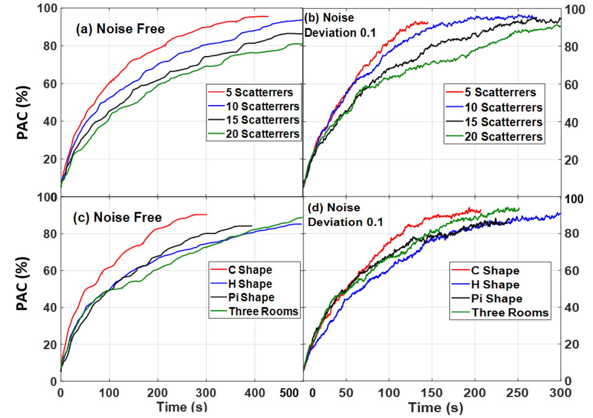
We considered environments with scatterrers (cf. Fig. 4), and walls (cf. Fig. 5), where Fig. 17 plots the PAC under the two most extreme noise-levels. As discussed before, high noise-levels tend improve the speed of the algorithm. The range of PAC reached by sensor nodes at different noise levels is within 5.0% (on the absolute coverage scale) between minimum and maximum values reached, demonstrating that BISON can handle noisy environment without dropping the coverage quality, all that while maintaining connected network.
6.3.3 Coverage in environments with crevices
By exploring performance in environments with narrow regions (depicted in Fig. 6) we address the issue of providing network coverage in difficult environments.
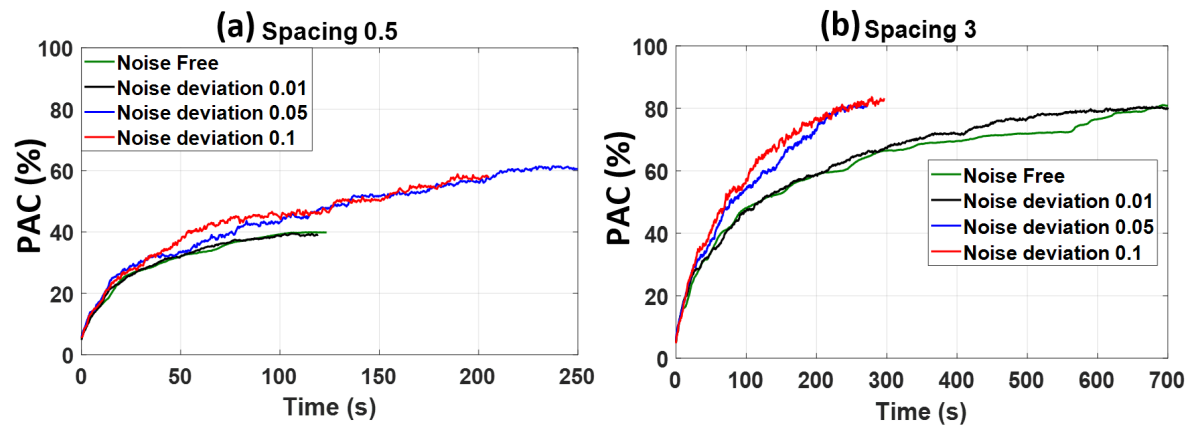
Fig. 18 plots the PAC obtained in these scenarios for spacing sized at 0.5 (narrow passage) and 3.0 (wide passage), cf. Fig. S12 in SOM for the remaining results.
For narrow spacing (e.g., 0.5), the presence of high noise deviations allows nodes to discover narrow areas due to substantial changes in the Voronoi regions and corresponding centroids generated, thus enabling nodes to cover more regions compared to noise-free or low noise levels.
6.3.4 Distribution of coverage uniformity
Above we compared performance during deployment using the distance traveled (cf. §6.2.4), which we translated into energy cost using the measure of kinetic energy (cf. Equation 6). Analogously, we do the same for the coverage provided, with the energy cost being encoded in the measure of coverage uniformity (cf. Equation 7), for which the smaller the value the better the performance.
The impact of noise on
The impact of obstacles on
Given the expected outcomes for the impact of increasing noise-levels, we investigate the impact of obstacles, Fig. 19, (c). Pillars obstruct deployment and impact coverage regions. As expected, increasing the number of obstacles slows down the convergence towards similar coverage. The final results are, however, comparable and differ only marginally. Additional results of for obstacle-rich environments are found in Figs. S13 and S14 in SOM.
for small elongated spaces
When deploying nodes into narrow spaces, their Voronoi regions are defined by the walls on either side, causing the final to be much higher; this is clearly visible in Fig. 19, (d). Furthermore, in the absence of noise cavities are not entered, allowing the WSN to deploy faster into the effectively smaller environment. More illustrative results are found in Fig. S15 in SOM.
6.4 Swarm-like Noise Coherence in BISON
Throughout the paper we have noticed a - somewhat counter-intuitive - impact of noise: increasing noise-levels resulted in better coverage and faster convergence (though at the cost of significantly larger distances traveled). We argue that this is due to noise-driven coherence in the collective motion of the WSN, which can be seen as a swarm of sensors with Voronoi-distributed domains.
To test this hypothesis, we analyzed the distribution of the diffusion- and drift-coefficients values (cf. [51]) for the sensor nodes as a function of the average velocity.
6.4.1 The impact of noise on performance
First of all, we confirm the consistent positive impact observed throughout the results: Fig. 20 shows this for our simulated environments with pillars (left) and walls (right), measuring the time to achieve 85% coverage, over the 4 noise-levels used.
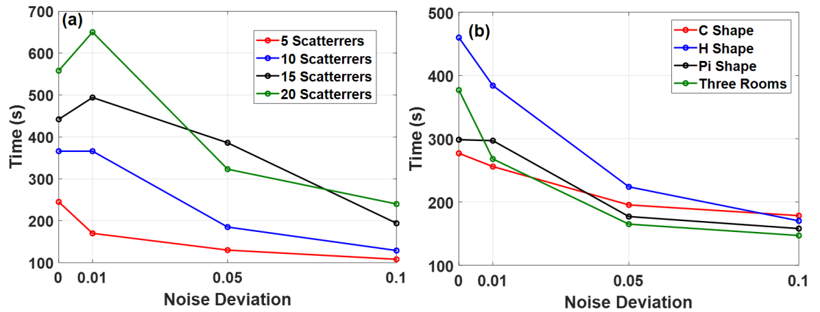
Upon reflection, the explanation for these results is actually straight-forward: increased noise results in increasingly erroneous node localization and, thus, centroid calculation. This in turn leads to increased movement to counter the perceived off-set, which constitutes a faster space exploration.
6.4.2 The impact of noise on collective motion
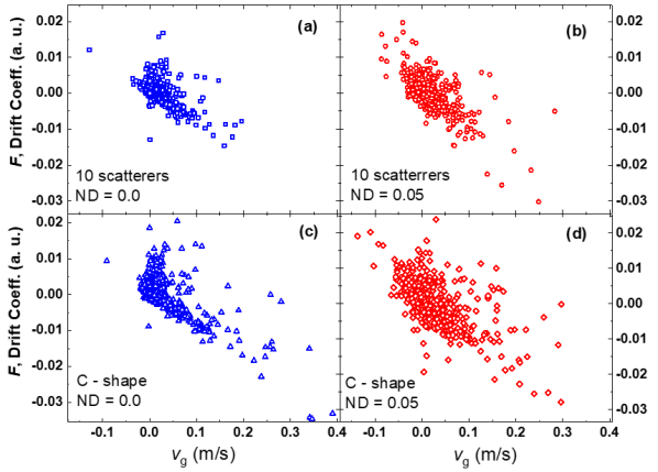
Collective motion of objects of both, biological and artificial nature, may correspond to various forms of coherence [51, 55, 56, 57, 58]. In the analysis of the influence of the presence of the controllable noise level presented in preceding sub-sections, it is evident that some of the parameters quantifying performance of the BISON algorithm show better performance with the presence of noise.
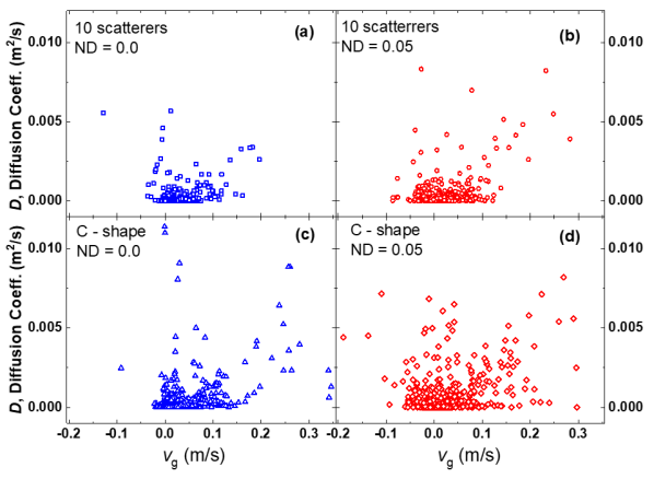
As discussed (§5.3), overall movement is investigated using node–diffusion (Eq. 3) and –drift (Eq. 4), the former representing the mean rate of change in average node velocity, the latter quantifying the evolution thereof. The results for walled environments (bottom) and environments with walls (top) are plotted in Fig. 21.
Similar plots from our other experiments all show similar or stronger differences in the spread of the instantaneous values of the diffusion coefficient. We believe that this finding is important for the design of collective robot swarms (who will always operate under noise in the real world), and will be subject of further reports. Similar to the differences in the distribution of the diffusion coefficient values, there are notable quantitative and qualitative differences in the distribution of the drift coefficient, as shown above. By increasing the noise-level we cause the broadening of the distribution. A similar impact is visible between different environments (comparing (a) vs (c) and (b) vs (d) in either), indicating that drift and diffusion can be used to deduce some ranking of difficulty on our environments.
6.5 Loss of Members and Collision-free Recovery
We also investigate the impact of node-loss as well as formulate a strategy to address it. As discussed in §4.4 we distinguish three types of nodes positions (side, corner and inside the collective), the nodes 3, 7 and 20, labelled in Fig. 22 are respective representatives thereof.
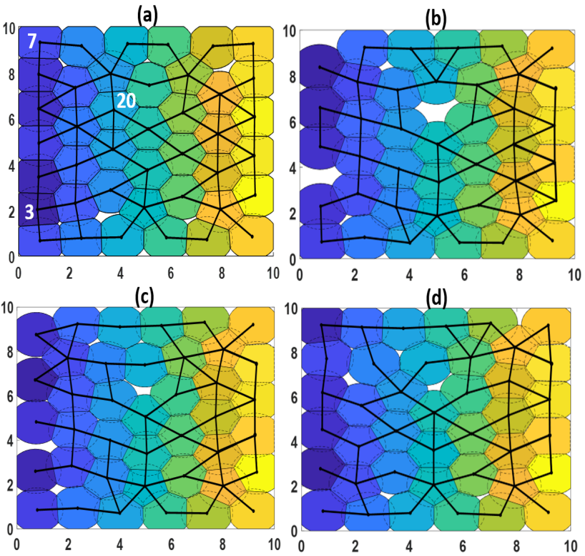
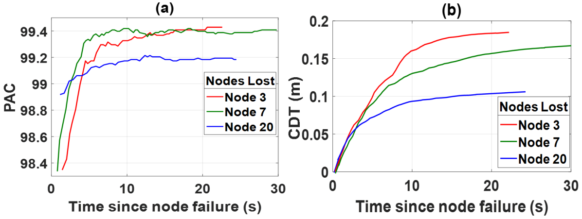
Fig. 22 (a) shows a WSN suffering triple node loss (b) with BISON recovering from the resulting loss of coverage. We simulated individual node loss and recorded the evolution of both, PAC as well as CDT during the recovery of the remaining network after the node-loss occurred. The results are plotted in Fig. 23: we see a quick recovery of the network noting that the relative position within the network has a large impact on the recovery process and performance.
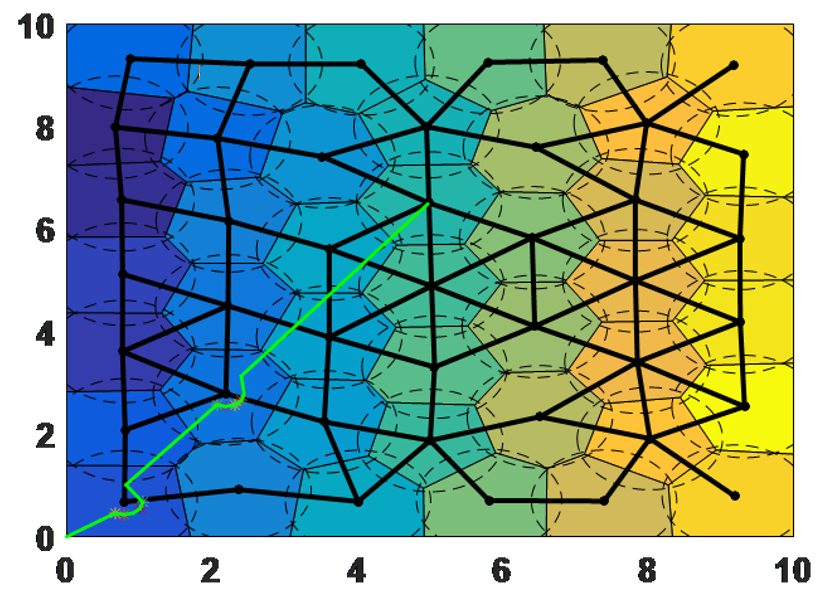
As part of our ongoing work, we start by simulating a short exit path for a randomly chosen node that lost most of its power, as shown in Fig. 24. Each node knows the location of the starting point where nodes are injected from. A direct path is then planned from the current node location towards the injection point. During the motion of the node, it will sense if there is another node within its sensing range that blocks the path and will avoid it by moving around that node until it is back again on the planned path.
The green line in Fig. 24 illustrates the shortest exit path a certain low power sensor node follows to get out of the network before it dies out. We will further extend the work to consider the total time required to exit the area and the amount of energy consumed during the exit process, as well as include some approach to guide nodes along the shortest path in the network (in case that there are obstacles or blocking the shortest direct path).
7 Conclusions and Future Work Plan
We presented BISON (Bio-inspired Self-organizing Network), a new Voronoi-based optimization algorithm for wireless sensor network deployment and reallocation in an unknown, obstacle-rich and noisy environment. One novel aspect of BISON is its ability to adapt to changes in the environment. A new method for node injection, guided by system requirements and based on satisfying coverage and connectivity conditions is proposed. Nodes calculate their Voronoi regions exclusively on the basis of locally available information and then continuously move towards the center of their region. A number of performance criteria were introduced and used to validate the algorithm.
A summary of the algorithm results is the following:
-
1.
In terms of the coverage and the number of nodes, BISON tends to achieve maximum coverage at an earlier time and with fewer nodes compared to the NSVA algorithm (with ratio of 1 to 3), under the same parameters. However, the average distance traveled is higher for BISON as new nodes enter the area of interest one at a time, while the NSVA algorithm tends to have a fixed number of nodes at the starting point waiting to be distributed in the network, implying that nodes need less movement during the deployment process.
-
2.
The algorithm was also evaluated in a variety of environments that contain different obstacle shapes, scattering objects, and spacings, showing the broad applicability of BISON while performing well in a variety of case studies.
-
3.
The presence of Gaussian noise allowed the sensor nodes to cover the region of interest faster than in a noise-free situation, and to reach the maximum coverage in shorter time.
-
4.
The early nodes consume the most energy as they are the first to discover the region of interest and the optimum position is not yet clear to them. As more nodes enter the area, their movements become limited and the optimum position becomes better determined, leading to the decrease of energy consumption with time. Additionally, in a noisy environment, a trade-off between the coverage efficiency and the energy expenditure is defined.
-
5.
Loss of some of the early nodes is analyzed, demonstrating robustness of the proposed BISON solution.
-
6.
Lastly, the influence of noise is analyzed within drift-diffusion framework, lending an insight into future design of efficient deployment networks.
Future work plan will consider the dynamics of the nodes’ entry that could be somewhat improved, as the density near the entry point needs to be optimized. Variable sensing range for individual sensors will also add a layer of realistic implementation to the algorithm, as will the inclusion of temporally varied noise levels. Finally, a three-dimensional consideration of the algorithm need to be studied to better visualize the performance of the algorithm and have a better evaluation for real implementations.
Acknowledgments
The authors acknowledge support from the UAE ICTFund grant “Bio-inspired Self-organizing Services”. AFI and DR acknowledge motivating discussion with Prof. V. Kumar (Univ. of Pennsylvania).
References
- [1] P. Tiwari, V. P. Saxena, R. G. Mishra and D. Bhavsar, “Wireless Sensor Networks: Introduction, Advantages, Applications and Research Challenges”, Open International Journal of Technology Innovations and Research, vol. 14, pp. 1-11, 2015.
- [2] L. Poudyal and B. Sen, “A Survey on Localization and Covering Techniques in Wireless Sensor Networks,” International Journal of Computer Applications, vol. 67, no. 7, pp. 23-27, 2013.
- [3] D. Ye, D. Gong and W. Wang, “Application of Wireless Sensor Networks in Environmental Monitoring,” in 2nd IEEE International Conference on Power Electronics and Intelligent Transportation System, Shenzhen, China, December 2009.
- [4] F. Guerriero, A. Violi, E. Natalizio, V. Loscri and C. Costanzo, “Modelling and Solving Optimal placement Problems in Wireless Sensor Networks,” Applied Mathematical Modelling, vol. 35, no. 1, pp. 230-241, 2011.
- [5] D. Chandirasekaran and T. Jayabarathi, “A Case Study of Bio-Optimization Techniques for Wireless Sensor Network in Node Location Awareness,” Indian Journal of Science and Technology, vol. 8, no. 31, pp. 1-9, 2015.
- [6] H. Ghayvat, S. Mukhopadhyay, X. Gui and N. Suryadevara, “WSN- and IoT-Based Smart Homes and Their Extension to Smart Buildings,” Sensors, vol. 15, pp. 10350-10379, 2015.
- [7] Z. Chuan, Z. Chunlin, S. Lei and H. Guangjie, “A Survey on Coverage and Connectivity Issues in Wireless Sensor Networks,” Journal of Network and Computer Applications, vol. 35, no. 2, pp. 619-632, 2012.
- [8] P. Sahu, and S. R. Gupta, “Deployment Techniques in Wireless Sensor Networks,” International Journal of Soft Computing and Engineering, vol. 2, no. 3, pp. 525-526, 2012.
- [9] S. Mnasri, N. Nasri and T. Val, “The Deployment in the Wireless Sensor Networks: Methodologies, Recent Works and Applications,” in International Conference on Performance Evaluation and Modeling in Wired and Wireless Networks (PEMWN 2014), Nov 2014, Sousse, Tunisia, Proceedings of PEMWN 2014 .
- [10] M. Kiran, K. Kamal, G. Nitin, “Application-based Study on Wireless Sensor Network,” International Journal of Computer Applications, vol. 21, no. 8, pp. 9-15, 2011.
- [11] M. Abbasi, M. S. Abd Latif and H. Chizari, “Bioinspired Evolutionary Algorithm Based for Improving Network Coverage in Wireless Sensor Networks,” The Scientific World Journal, vol. 2014, pp. 1-8, 2014.
- [12] Q. Du, V. Faber and M. Gunzburger, “Centroidal Voronoi Tessellations: Applications and Algorithms,” SIAM Review, vol. 41, no. 4, pp. 637-676, 1999.
- [13] K. Eledlebi, D. Ruta, F. Saffre, Y. Al Hammadi and A. F. Isakovic, “A Model for Self-deployment of Autonomous Mobile Sensor Network in an Unknown Indoor Environment,” in Ad Hoc Networks: 9th International Conference (AdHocNets 2017), Proceedings, Niagara Falls, ON, Canada, Springer, pp. 208-215, 2017.
- [14] M. A. Adnan, M. Abdur Razzaque, I. Ahmed and I. F. Isnin, “Bio-mimic Optimization Strategies in Wireless Sensor Networks: A Survey,” Sensors, vol. 14, pp. 299-345, 2014.
- [15] T. Sheltami, A. Mahmoud, K. Alsafari and E. shakshuki, “Self-Organizing Sensor Networks Coverage Problem,” in IEEE 26th Biennial Symposium on Communications (QBSC), Kingston, ON, Canada, May 2012.
- [16] T. Watteyne, “Energy-efficient Self-organization in Wireless Sensor Networks,” PhD thesis manuscript, INSA Lyon, 2008.
- [17] A. Norouzi and A. H. Zaim, “Genetic Algorithm Application in Optimization of Wireless Sensor Networks,” The Scientific World Journal, vol. 2014, pp. 1-15, 2014.
- [18] R. Klein, “Voronoi Diagrams and Delaunay Triangulations,” in Encyclopedia of Algorithms, NewYork, Springer Science and Business Media, ISBN: 9789814447645, pp. 1-5, 2014.
- [19] M. Hasegawa and T. Masaharu, “On the Pattern of Space Division by Territories,” Annuals of the Institute of Statistical Mathematics, vol. 28, no. 1, pp. 509-519, December 1976.
- [20] H.-J. Lee, Y.-H. Kim, Y.-H. Han and C. Y. Park, “Centroid-based Movement Assisted Sensor Deployment Schemes in Wireless Sensor Networks,” in Vehicular Technology Conference, USA, Fall 2010.
- [21] A. Pietrabissa, F. Liberati and G. Oddi, “A Distributed Algorithm for Ad-hoc Network Partitioning Based on Voronoi Tessellation,” Elsevier: Ad Hoc Networks, vol. 46, pp. 37-47, 2016.
- [22] M. A. M. Vieira, L. F. M. Vieira, L. B. Ruiz, A. Loureiro, A. Fernandes and J. Nougueira, “Scheduling Nodes in Wireless Sensor Networks: A Voronoi Approach,” in 28th Annual IEEE International Conference on Local Computer Networks, 2003. LCN ’03. Proceedings., Bonn/Konigswinter, Germany, 2003.
- [23] O. Banimelhem, M. Mowafi and W. Aljoby, “Genetic Algorithm Based Node Deployment in Hybrid Wireless Sensor Network,” Communications and Network, vol. 5, pp. 273-279, 2013.
- [24] S. Kaur and R. Uppal, “Dynamic Deployment of Homogeneous Sensor Nodes Using Genetic Algorithm with Maximum Coverage,” in 2nd International Conference on Computing for Sustainable Global Development, New Delhi, India, 2015.
- [25] Yipeng Qu and Stavros V. Georgakopoulos, “A Centralized Algorithm for Prolonging the Lifetime of Wireless Sensor Networks using Particle Swarm Optimization,” in IEEE Wireless and Microwave Technology Conference (WAMICON), Florida, USA, April 2012.
- [26] N. Rahmani, F. Nematy, A. M. Rahmani and M. Hosseinzadeh, “Node Placement for Maximum Coverage Based on Voronoi Diagram Using Genetic Algorithm in Wireless Sensor Networks,” Australian Journal of Basic and Applied Sciences, vol. 5, no. 12, pp. 3221-3232, 2011.
- [27] N. A. B. Ab Aziz, A. W. Mohemmed and B. D. Sagar, “Particle Swarm Optimization and Voronoi Diagram for Wireless Sensor Networks Coverage Optimization,” in IEEE International Conference on Intelligent and Advanced Systems, Kuala Lumpur, Malaysia, November 2007.
- [28] G. Wang, G. Cao and T. L. Porta, “Movement-Assisted Sensor Deployment,” IEEE Transactions on Mobile Computing, vol. 5, no. 6, pp. 640-652, 2006.
- [29] D. Wang, B. Xie and D. P. Agrawali, “Coverage and Lifetime Optimization Of Wireless Sensor Networks With Gaussian Distribution,” IEEE Transactions on mobile computing, vol. 7, no. 12, pp. 1444-1458, 2008.
- [30] M. R. Senouci, A. Mellouk, K. Asnoune and F. Y. Bouhidel, “Movement-Assisted Sensor Deployment Algorithms: A Survey and Taxonomy,” IEEE Communication Surveys and Tutorials, vol. 17, no. 4, pp. 2493-2510, 2015.
- [31] J. Stergiopoulos and A. Tzes, “Voronoi-based Coverage Optimization for Mobile Networks with Limited Sensing Range - A Directional Search Approach,” in American Control Conference, Missouri, USA, 2009.
- [32] J. Zou, J. Kusyk, M. U. Uyar, S. Gundry and C. S. Sahin, “Bio-inspired and Voronoi-based Algorithms for Self-positioning Autonomous Mobile Nodes,” in IEEE Military Communications Conference (MILCOM 2012), Orlando, FL, USA, October 2009.
- [33] J. Zou, S. Gundry, J. Kusyk, C. S. Sahin and M. U. Uyar, “Bio-inspired and voronoi-based algorithms for self-positioning of autonomous vehicles in noisy environments,” in Proceedings of the 8th International Conference on Bio-inspired Information and Communications Technologies, Boston, Massachusetts, pp. 12-22, Dec 2014.
- [34] J. Kusyk, J. Zou, S. Gundry, C. S. Sahin and M. U. Uyar, “Metrics for Performance Evaluation of Self-positioning Autonomous MANET Nodes,” in 35th IEEE Sarnoff Symposium, Newark, NJ, USA, June 2012.
- [35] S. Gundry, J. Zou, C. S. Sahin, J. Kusyk and M. U. Uyar, “Autonomous and Fault Tolerant Vehicular Self Deployment Mechanisms in MANETs,” in IEEE International Conference on Technologies for Homeland Security, Waltham, MA, USA, November 2013.
- [36] N. Bartolini, T. Calamoneri, T. F. La Porta and S. Silvestri, “Autonomous Deployment of Heterogeneous Mobile Sensors,” IEEE Transactions on Mobile Computing, vol. 10, no. 6, pp. 753-766, 2011.
- [37] Y. Kantaros, M. Thanou and A. Tzes, “Distributed Coverage Control for Concave Areas by a Heterogeneous Robot-swarm with Visibility Sensing Constraints,” Elsevier: Automatica, vol. 53, pp. 195-207, 2015.
- [38] H. Imai, M. Iri and K. Murota, “Voronoi Diagram in the Laguerre Geometry and its Applications,” Society for Industrial and Applied Mathematics, vol. 14, no. 1, pp. 93-105, 1985.
- [39] H. Mahboubi and A. G. Aghdam, “Distributed Deployment Algorithms for Coverage Improvement in a Network of Wireless Mobile Sensors: Relocation by Virtual Force,” IEEE Transactions on Control of Network Systems, vol. PP, no. 99, pp. 1-19, 2016.
- [40] H. Mahboubi, K. Moezzi, A. G. Aghdam and K. Sayrafian-Pour, “Distributed Sensor Coordination Algorithms for Efficient Coverage in a Network of Heterogeneous Mobile Sensors,” IEEE Transactions on Automatic Control, vol. 62, no. 11, pp. 5954-5961, 2017.
- [41] N. Bartolini, S. Ciavarella, S. Silvestri and T. La Porta, “On the Vulnerabilities of Voronoi-based Approaches to Mobile Sensor Deployment,” IEEE Transactions on Mobile Computing, vol. 15, no. 12, pp. 3114-3128, 2016.
- [42] N. Bartolini, T. Calamoneri, E. G. Fusco, A. Massini and S. Silvestri, “Autonomous Deployment of Self-organizing Mobile Sensors for a Complete Coverage,” Springer: International Workshop on Self-organizing Systems, pp. 194-205, 2008.
- [43] N. Bartolini, T. Calamoneri, S. Ciavarella, T. La Porta and S. Silvestri, “Autonomous Mobile Sensor Placement in Complex Environments,” ACM Transactions on Autonomous and Adaptive Systems, vol. 12, no. 2, pp. 1-28, 2017.
- [44] L. Liu, G. Han, H. Wang and J. Wan, “Obstacle-avoidance Minimal Exposure Path for Heterogeneous Wireless Sensor Networks,” Ad Hoc Networks Journal, vol. 55, pp. 50-61, 2016
- [45] J. Cortes, S. Martinez, T. Karatas and F. Bullo, “Coverage Control for Mobile Sensing Networks,” IEEE Transactions on Robotics and Automation, vol. 20, no. 2, pp. 243-255, 2004.
- [46] S. L. Mohammed, “Distance Estimation Based on RSSI and Log-normal Shadowing Models for ZigBee Wireless Sensor Network,” Engineering and Technology Journal, vol. 34, no. 15, pp. 2950-2960, 2016.
- [47] H. Chenji and R. Stoleru, “Toward Accurate Mobile Sensor Network Localization in Noisy Environments,” IEEE Transactions on mobile computing, vol. 12, no. 6, pp. 1-14, June 2013.
- [48] H. Zhang and J. C. Hou, “Maintaining Sensing Coverage and Connectivity in Large Sensor Networks,” Ad Hoc and Sensor Wireless Networks Journal, vol. 1, no. 1–2, pp. 89–124, 2005.
- [49] Y.-C. Wang, C.-C. Hu and Y.-C. Tseng, “Efficient Deployment Algorithms for Ensuring Coverage and Connectivity of Wireless Sensor Networks,” in First International Conference on Wireless Internet, Budapest, Hungary, July 2005.
- [50] A. Ohya, T. Ohno and S. Yuta, “Obstacle Detectability of Ultrasonic Ranging System and Sonar Map Understanding,” Elsevier: Robotics and Autonomous Systems, vol. 18, no. 1-2, pp. 251-257, 1996.
- [51] C. A. Yates, R. Erban, C. Escudero, I. D. Couzin, J. Buhl, I. G. Kevrekidis, P. K. Maini and D. J. T. Sumpter, “Inherent Noise Can Facilitate Coherence in Collective Swarm Motion,” Proceedings of the National Academy of Sciences in the United States of America, vol. 106, no. 14, pp. 5464-5469, 2009.
- [52] G. Nimisha, B. Indrajit and S. Tuhina, “Energy Efficient Coverage of Static Sensor Nodes Deciding on Mobile Sink Movements Using Game Theory,” in IEEE Conference on Applications and Innovations in Mobile Computing, Kolkata, February 2014.
- [53] M. Abo-Zahhad, N. Sabor, S. Sasaki and S. M. Ahmed, “A Centralized Immune-Voronoi Deployment Algorithm for Coverage Maximization and Energy Conservation in Mobile Wireless Sensor Networks,” Information Fusion Journal, vol. 30, pp. 36-51, 2015.
- [54] A. Khelil and R. Beghdad, “ESA: an Efficient Self-deployment Algorithm for Coverage,” in The 7th International Conference on Emerging Ubiquitous Systems and Pervasive Networks, London, UK, September 2016.
- [55] J. Parrish, S. V. Viscido and D. Grunbaum, “Self-Organized Fish Schools: An Examination of Emergent Properties,” The Biological Bulletin Journal, vol. 202, no. 3, pp. 296-305, 2002.
- [56] V. Gabor, C. Viragh, G. Somorjai, N. Tarcai, T. Szorenyi, T. Nepusz and T. Vicsek, “Outdoor Flocking and Formation Flight with Autonomous Aerial Robots,” in IEEE International Conference on Intelligent Robots and Systems, 2014.
- [57] N. W. F. Bode, D. W. Franks and A. J. Wood, “Making Noise: Emergent Stochasticity in Collective Motion,” Journal of Theoretical Biology, vol. 267, no. 3, pp. 292-299, 2010.
- [58] B. Blonder, T. A. Wey, A. Dornhaus, R. James and A. Sih, “Temporal Dynamics and Network Analysis,” Journal of Methods in Ecology and Evolution, vol. 3, no. 6, pp. 958-972, 2012.
- [59] F. Aurenhammer, R. Klein and D.-T. Lee, “Voronoi Diagrams and Delaunay Triangulations,” Singapore: World Scientific, 2013.
Biographies
Khouloud Eledlebi
Biography will be added for final version.
Dymitr Ruta
Biography will be added for final version.
Hanno Hildmann
Biography will be added for final version.
Fabrice Saffre
Biography will be added for final version.
Yousof Al Hammadi
Biography will be added for final version.
A.F. Isakovic
Biography will be added for final version.
Supporting Online Materials
Additional results, supporting the findings and statements in the text as well as some animations, are available from the corresponding author, upon reasonable request