Checking individuals and sampling populations
with imperfect tests

Abstract

In the last months, due to the emergency of Covid-19, questions related to the fact of belonging or not to a particular class of individuals (‘infected or not infected’), after being tagged as ‘positive’ or ‘negative’ by a test, have never been so popular. Similarly, there has been strong interest in estimating the proportion of a population expected to hold a given characteristics (‘having or having had the virus’). Taking the cue from the many related discussions on the media, in addition to those to which we took part, we analyze these questions from a probabilistic perspective (‘Bayesian’), considering several effects that play a role in evaluating the probabilities of interest. The resulting paper, written with didactic intent, is rather general and not strictly related to pandemics: the basic ideas of Bayesian inference are introduced and the uncertainties on the performances of the tests are treated using the metrological concepts of ‘systematics’, and are propagated into the quantities of interest following the rules of probability theory; the separation of ‘statistical’ and ‘systematic’ contributions to the uncertainty on the inferred proportion of infectees allows to optimize the sample size; the role of ‘priors’, often overlooked, is stressed, however recommending the use of ‘flat priors’, since the resulting posterior distribution can be ‘reshaped’ by an ‘informative prior’ in a later step; details on the calculations are given, also deriving useful approximated formulae, the tough work being however done with the help of direct Monte Carlo simulations and Markov Chain Monte Carlo, implemented in R and JAGS (relevant code provided in appendix).

“Grown-ups like numbers”
(The Little Prince)

“The theory of probabilities is basically
just common sense reduced to calculus”
(Laplace)

“All models are wrong, but some are useful”
(G. Box)

References   .   .   .   .   .   .   .  .  .    .   .   .   .   .   .   .  .  .    .   .   .   .   .   .   .  .  .   .   96
Appendix A – Some remarks on ‘Bayes’ formulae’   .   .   .   .   .   .   .  .  .  99
Appendix B – R and JAGS code   .   .   .   .   .   .   .  .  .    .   .   .   .   .   .   .  .   103

1 Introduction

The Covid-19 outbreak of these months raised a new interest in data analysis, especially among lay people, for long locked down and really flooded by a tidal wave of numbers, whose meaning has often been pretty unclear, including that of the body counting, which should be in principle the easiest to assess. As practically anyone who has some experience in data analysis, we were also tempted – we have to confess – to build up some models in order to understand what was going on, and especially to forecast future numbers. But we immediately gave up, and not only because faced with numbers that were not really meaningful, without clear conditions, within reasonable uncertainty, about how they were obtained. The basic question is that, we realized soon, we cannot treat a virus spreading in a human population like a bacterial colony in a homogeneous medium, or a continuous (or discretized) thermodynamic system. People live – fortunately! – in far more complex communities (‘clusters’), starting from the families, villages and suburbs; then cities, regions, countries and continents of different characteristics, population densities and social behaviors. Then we would have to take into account ‘osmosis’ of different kinds among the clusters, due to local, intermediate and long distance movements of individuals. Not to speak of the diffusion properties of viruses in general and of this one in particular.

A related problem, which would complicate further the model, was the fact that tests were applied, at least at the beginning of pandemic, mainly to people showing evident symptoms or at risk for several reasons, like personnel of the health system. We were then asking ourselves rather soon, why tests were not also made on a possibly representative sample of the entire population, independently of the presence of symptoms or not. This would be, in our opinion, the best way to get an idea of the proportion of the population affected at a given ‘instant’ (to be understood as one or a few days) and to take decisions accordingly. It is quite obvious that surveys of this kind would require rather fast and inexpensive tests, to the detriment of their quality, thus unavoidably yielding a not negligible fraction of so called false positives and false negatives.

When we read in a newspaper [2] about a rather cheap antibody blood test able to tag the individuals being or having been infected  we decided to make some exercises in order to understand whether such a ‘low quality’ test would be adequate for the purpose and what sample size would be required in order to get ‘snapshots‘ of a population at regular times. In fact Ref. [2] not only reported the relevant ‘probabilities’, namely 98% to tag an Infected (presently or previously) as Positive (‘sensitivity’) and 88% to tag a not-Infected as Negative (‘specificity’), but also the numbers of tests from which these two numbers resulted. This extra information is important to understand how believable these two numbers are and how to propagate their uncertainty into the other numbers of interest, together with other sources of uncertainty. This convinced us to go through the exercise of understanding how the main uncertainties of the problem would affect the conclusions:

• uncertainty due to sampling;

• uncertainty due to the fact that the above probabilities differ from 1;

• uncertainty about the exact values of these ‘probabilities’.

Experts might argue that other sources of uncertainty should be considered, but our point was that already clarifying some issues related to the above contributions would have been of some interest. From the probabilistic point of view, there is another source of uncertainty to be taken into account, which is the prior distribution of the proportion of infectees in the population, however not as important as when we have to judge from a single test if an individual is infected or not.

The paper, written with didactic intent (and we have to admit that it was useful to clarify some issues even to us), is organized in the following way.

• Section  2 shows some simple evaluations based on the nominal capabilities of the test, without entering in the probabilistic treatment of the problem. The limitations of such ‘rough reasoning’ become immediately clear.

• Then we move in Sec. 3 to probabilistic reasoning, applied to the probability that a person tagged as positive/negative ‘is’ (or ‘has been’) really infected or not infected. The probabilistic tool needed to make this so called ‘probabilistic inversion’ (Bayes’ theorem) is then reminded and applied, showing the relevance of the probability that the individual is infected or not, based on other pieces of information/knowledge (‘prior probability’), a fundamental ingredient of inference often overlooked.

• The effect of the uncertainty on sensititivity, specificity and proportion of infectees in the population is discussed in Sec. 4. But, before doing that, we have to model the probability density function for these uncertain quantities. Hence an introduction to the application of Bayes’ theorem to continuous quantities is required, including some notes on the use of conjugate priors.

• From Sec. 5 we switch our focus from single individuals to populations. Our aim, that is inferring the proportion of ‘infectees’ (meaning, let us repeat it once more, ‘individuals being or having being infected’) will be reached in Secs. 8 and 9. But, for didactic purposes, we proceed by step, starting from the expected number of positives, examining in depth the various sources of uncertainty. In particular, in Sec. 7 we study the measurability of $p$ and the dependence of its ‘resolution power’ on the test performances and the sample size. Most of the work is done using Monte Carlo methods, but some useful approximated formulae for the evaluation of uncertainty on the result are given as well.

• The probabilistic inference of $p$, that is evaluating its probability density function $f(p)$, conditioned by data and well stated hypotheses, is finally done in Sec. 8. Having to solve a multidimensional problem, in which $f(p)$ is finally obtained by marginalization, Markov Chain Monte Carlo (MCMC) methods become a must. In particular, we use JAGS [10], interfaced with R [11] through the package rjags [12]. We also evaluate, by the help of JAGS, some joint probability distributions and the correlation coefficients among the variables of interest, thus showing the great power of MCMC methods, that have given a decisive boost to Bayesian inference in the past decades.

• However, we show in Sec. 9 how to solve the problem exactly, although not in closed form, and limiting ourselves to the pdf of $p$. A simple extension of the expression of the normalization constant allows to evaluate the first moments of the distribution, from which expected value, variance, skewness and kurtosis can be computed (and then an approximation of $f(p)$ can be ‘reconstructed’).

• An important issue, also of practical relevance, is the inference of the proportions of infectees in different populations, analyzed in Sec. 8.6, after having been anticipated in Sec. 7.4. In fact, since the uncertainties about sensitivity and specificity act as systematic errors (hereafter ‘systematics’), the differences between these proportions can be determined better than each of them.

• The role of the prior in the inference of $p$, already analyzed in detail in Sec. 8.7, is discussed again in Sec. 9.4, with particular emphasis to the case in which priors are at odds ‘with the data’ (in the sense specified there). The take away message will be to be very careful in taking literally ‘comfortable’ mathematical models, never forgetting the quotes by Laplace and Box reminded in the front page.

Two appendixes complete the paper. Appendix A is a kind of summary of ‘Bayesian formulae’, with emphasis on the practical importance of unnormalized posteriors obtained by a suitable choice of the so called chain rule of probability theory and on which most Monte Carlo methods to perform Bayesian inference are based. In Appendix B several R scripts are provided in order to allow the reader to reproduce most of the results presented in the paper.

2 Rough reasoning based on expectations

2.1 Setting up the problem

Let us imagine we have a population of $N$ elements, a proportion $p$ of which shares a given character. The simplest example is that of a box containing $N$ balls, $n_{1}$ white and $n_{2}$ black. Let $p$ be the proportion of white balls, i.e. $p=n_{1}/N$. If we extract at random $m$ balls, then we roughly expect $m_{1}\approx n_{1}\times m/N=p\cdot m$ white and $m_{2}\approx n_{2}\times m/N=(N-n_{1})\times m/N=(1-p)\cdot m$ black. A classical problem in probability theory is to infer the proportion $p$ from the observed (‘measured’) proportion $p_{m}=m_{1}/m$.

Obviously, if $m$ is equal to $N$, i.e. if we completely empty the box, then we acquire full knowledge of the box content and the solution is trivial. However, in most cases we are unable to analyze the entire population and we have to infer $p$ from a sample. Therefore, although $p_{m}$ can be a reasonable rough estimate of $p$, we can never be sure about the true proportion. At most, there are numerical values we shall believe more (those around $p_{m}$) and others we shall believe less. This problem was first tackled analytically by Laplace in 1774 [13].

Let us now complicate the problem, taking into account the fact that we are not even sure about the characteristics of each sampled individual, as, instead, it happens with black and white balls. This is exactly what happens with infections of different kinds, unless the symptoms are so evident and unique to rule out any other explanation. We have then to rely on tests that are typically not perfect, especially if we have neither time nor money to inspect in detail each individual in order to really see the active agent. Sticking to tests providing only a binary response, as we hear and read in the media, and assuming that such testing devices and procedures are planned to detect the infected individuals, we expect that if the answer is positive then there should be a quite high chance that the individual is really infected, and a small chance that she is not. Similarly, if the answer is negative, there should be a high chance that the individual is not infected. (The conditionals are due to the fact that there are other pieces of information to take into account, as we shall see.)

We can characterize therefore the test by two virtually continuous numbers $\pi_{1}$ and $\pi_{2}$ in the range between 0 an 1 such that, depending on whether the individual is infected or not, the test procedure provides positive and negative answers with probabilities

$$P(\mbox{Pos}\,|\,\mbox{Inf}) = \pi_{1}$$

$$P(\mbox{Neg}\,|\,\mbox{Inf}) = 1-\pi_{1}\,;$$

$$P(\mbox{Pos}\,|\,\mbox{NoInf}) = \pi_{2}$$

$$P(\mbox{Neg}\,|\,\mbox{NoInf}) = 1-\pi_{2}\,,$$

with self-evident meaning of the symbols (we just remind that the ‘$|$’ indicates that what follows it plays the role of conditions and therefore ‘$|$’ should be read as “under the condition”, or “conditioned by”). More technically, $\pi_{1}$ is defined as test sensitivity, while $(1-\pi_{2})$ is the test specificity (see e.g. Ref. [14]). Therefore, in order to fix the ideas, the test to which we are referring [2] has 98% sensitivity and 88% specificity.

As it is easy to understand, the numerical quantities of $\pi_{1}$ and $\pi_{2}$ do not come from first principles, but result from previous measurements. They are therefore affected by uncertainty as all results in measurements typically are [15]. Therefore, probability distributions have to be associated also to the possible numerical values of these two test parameters. Anyway, within this section we take the freedom to use their nominal values of 0.98 and 0.12 for our first rough considerations.

2.2 Fraction of sampled positives being really infected or not

Putting all together, our rough expectation is that our sample of $m$ individuals will contain $m_{1}\approx p\cdot m$ infected, although we shall write it within this section as an equality (‘$m_{1}=p\cdot m$’), and ditto for other related numbers. Out of these $m_{1}$ infected, $\pi_{1}\cdot m_{1}$ will be tagged as positive and $(1-\pi_{1})\cdot m_{1}$ as negative. Of the remaining $m_{2}=(1-p)\cdot m$, not infected, $\pi_{2}\cdot m_{2}$ will be tagged as positive and $(1-\pi_{2})\cdot m_{2}$ as negative. In sum, the expected numbers of positive and negative will be

$$n_{P} = \pi_{1}\cdot m_{1}+\pi_{2}\cdot m_{2}$$ (1)

$$n_{N} = (1-\pi_{1})\cdot m_{1}+(1-\pi_{2})\cdot m_{2}\,,$$ (2)

which we can rewrite as

$$n_{P} = \pi_{1}\cdot p\cdot m+\pi_{2}\cdot(1-p)\cdot m$$ (3)

$$n_{N} = (1-\pi_{1})\cdot p\cdot m+(1-\pi_{2})\cdot(1-p)\cdot m\,,$$ (4)

So, just to fix the ideas with a numerical example and sticking to $\pi_{1}=0.98$ and $\pi_{2}=0.12$ of Ref. [2], in the case we sample 10000 individuals we get, assuming 10% infected ($p=0.10$),

• number of infected in the sample: 1000 (and hence 9000 not infected);

• infected tagged as positive: 980;

• infected tagged as negative: 20;

• not infected tagged as positive: 1080;

• not infected tagged as negative: 7920;

• total number of positive: 2060;

• total number of negative: 7940;

• fraction of the positives really infected: $980/2060=47.6\,\%$.

2.3 Fraction of infectees in the positive sub-sample

We see therefore that, contrary to naive intuition, in spite of the apparent rather good quality of the test ($\pi_{1}=0.98$), the result is quite unreliable on the individual base: a positive person has roughly 50 % chance of being really infected. But this does not mean that the test was really useless. It has indeed increased the probability of a randomly chosen individual to be infected from 10% to 48%. On the contrary, the fraction of negatives really not infected is $7920/7940=99.75\%$. This result is also surprising on a first sight, being the specificity $(1-\pi_{2})$ only 88%, i.e. not ‘as good’ as the sensitivity $(\pi_{1})$, as high as 98%. We shall see the reason in a while. For the moment we just remark that in this second case the probability of a randomly chosen individual to be not infected has increased from 90 % to 99.75 %.

The reason of these counter-intuitive results is due to the role of the prior probability of being infected or not, based on the best knowledge of the proportion of infected individuals in the entire population. The easy explanation is that, given the numbers we are playing with, the number of positives is strongly ‘polluted’ by the large background of not infected individuals.

In order to see how the outcomes depend on $p$, let us lower its value from 10% to 1%. In this case our expectation will be of 1286 positives, out of which only 98 infected and 1188 not infected (the details are left as exercise). The fraction of positives really infected becomes now only 7.6 %. On the other hand the fraction of negatives really not infected is as high as 99.98 %. Figure 1

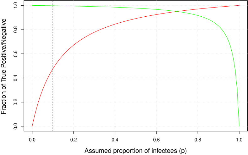
Figure 1: Fraction of ‘true positives’ (red line, starting at 0 for $p=0$) and ‘true negatives’ (green line, starting at 1 for $p=0$) in the sample, as a function of the assumed proportion $p$ of infected individuals in the population, assuming $\pi_{1}=P(\mbox{Pos}\,|\,\mbox{Inf})=0.98$ and $\pi_{2}=P(\mbox{Pos}\,|\,\mbox{NoInf})=0.12$ . The results in correspondence of $p=0.1$, arbitrarily used as reference value in the numerical example of this section, are marked by the vertical dashed line.

shows how these numbers depend on the assumed proportion of infectees in the population (and then in the sample, because of the rough reasoning we are following in this section).

This should make definitively clear that the probabilities of interest not only depend, as trivially expected, on the performances of the test, summarized here by $\pi_{1}$ and $\pi_{2}$, but also – and quite strongly! – on the assumed proportion of infectees in the population. More precisely, they depend on whether the individual shows symptoms possibly related to the searched for infection and on the probability that the same symptoms could arise from other diseases. However we are not in the condition to enter into such ‘details’ in this paper and shall focus on random samples of the population. Therefore, up to Sec 4.5, in which we deal with the probability that a tested individual is infected or not on the basis of the test result, we shall refer to $p$ as ‘proportion of infectees’ in the population. But everything we are going to say is valid as well if $p$ is our ‘prior’ probability that a particular individual is infected, based on our best knowledge of the case.

2.4 Estimating the proportion of infectees in the population

Now, after having seen what we can tell about a single individual chosen at random and of which we have no information about possible symptoms, contacts or behavior, let us see what we can tell about the proportion $p$ of infected in the population, based on the tests performed on the sampled individuals. The first idea is to solve Eqs. (3) and (4) with respect to $p$, from which it follows

$$p = \frac{n_{P}-\pi_{2}\cdot m}{(\pi_{1}-\pi_{2})\cdot m}\,.$$ (5)

Applying this formula to the 2060 positives got in our numerical example we re-obtain the input proportion of 10%, somehow getting reassured about the correctness of the reasoning. If, instead, we get more positives, for example 2500, 3000 or 3500, then the proportion would rise to 15.1%, 20.1% and 26.7%, respectively, which goes somehow in the ‘right direction’. If, instead, we get less, for example 2000 or 1500, then the proportion lowers to 9.3% and 3.5%, respectively, which also seems to go into the right direction.

However, keeping lowering the number of positives something strange happens. For $n_{P}=1200$ Eq. (5) vanishes and it becomes even negative for smaller numbers of positives, which is something concerning, indicating that the above formula is not valid in general. But why did it nicely give the exact result in the case of 2060 positives? And what is the reason why it yields negative proportions below 1200 positives? Moreover, Eq. (5) has a worrying behavior of diverging for $\pi_{1}=\pi_{2}$, even though irrelevant in practice, because such a test would be ridiculous – the same as tossing a coin to tag a person Positive or Negative (but in such a case we would expect to learn nothing from the ‘test’, certainly not that the real proposition of infectees diverges!).

Let us see the limits of validity of the equation.

• The lower limit $p\geq 0$ implies, as we have already seen in the numerical example, $n_{P}\geq\pi_{2}\cdot m$ and $\pi_{1}>\pi_{2}$.

• The upper limit $p\leq 1$ is reflected in the condition $n_{P}\leq\pi_{1}\cdot m$ (and $\pi_{1}>\pi_{2}$). In our numeric example this would mean to have less than 9800 positives in our sample of 10000. But this ignores the fact that the proportion of infectees in the sample could be higher than that in the population.

Anyway, it is clear that when the model contemplates probabilistic effects we have to use sound methods based on probability theory.

2.5 Moving to probabilistic considerations

Let us start seeing what is going on when there are no infected individuals in the population, i.e. when $p=0$. In our rough reasoning none of the 10000 sampled individual will be infected. But 12% of them will be tagged as positive, exactly the critical value of 1200 we have seen above. In reality we have neglected the fact that 1200 is an expectation, in the probabilistic meaning of expected value, but that other values are also possible. In fact, given the assumed properties of the test, the number of individuals which shall result positive to the test is uncertain, and precisely described by the well known binomial distribution with ‘probability parameter’ (see Ref. [5] for clarifications) $\pi_{2}$. The expectation has therefore an uncertainty, that we quantify with the standard uncertainty [15], i.e. the standard deviation of the related probability distribution. Using the well known formula resulting from the binomial distribution, which in our case reads as $\sigma=\sqrt{\pi_{2}\cdot(1-\pi_{2})\cdot m}$, we get, using our numbers, $\sigma=32.5$. Since we are dealing with reasonably large numbers, the Gaussian approximation holds and we can easily calculate that there is about 16% probability to get a number of positives equal or below 1167, and so on. In particular we get 0.1% probability to observe a number equal or below 1100, which we could consider a safe limit for practical purposes.

But, unfortunately, the story is a bit longer. In fact we don’t have to forget that $\pi_{2}$ comes itself from measurements and is therefore uncertain. Therefore, although 0.12 is its ‘nominal value’, also values below 0.10 are easily possible, yielding e.g. an expected number of positives, among the not infected individuals, of $1000\pm 30$ for $\pi_{2}=0.10$ and $800\pm 27$ for $\pi_{2}=0.08$ (hereafter, unless indicated otherwise, we quote standard uncertainties).

Then there is the question that we apply the tests on the sample, and not on the entire population. Therefore, unless the proportion of infectees in the population is exactly 0 or 1, the proportion of infectees in the sample (‘$p_{s}$’), will differ from $p$. For example, sticking to a reference $p=0.1$, in the 10000 individuals sampled from a population ten times larger we do not expect exactly 1000 infected, but $1000\pm 28$ as we shall see in detail in Sec. 6.1 (we only anticipate, in answer to somebody who might have quickly checked the numbers, that the standard uncertainty differs from 30, calculated from a binomial distribution, because this kind of sampling belongs, contrary to the binomial, to the model ‘extraction without reintroduction’).

2.6 Summing up

The simple reasoning based on mean expectations leads to correct results only when all probabilistic effects are negligible, an approximation which holds, generally speaking, only for ‘large numbers’. Under this approximation the numbers of individuals tagged as Positive or Negative can be considered to follow in a deterministic way from the assumptions, one of which is the proportion of infectees. This number can then be obtained inverting the deterministic relation, thus yielding Eq. (5). But when fluctuations around the mean expectations become important we need to use probability theory in order to infer the parameter of interest.

As far as telling from a single test if a person tagged as Positive is really infected, we have seen that the prior ‘assumed proportion’ of infected individuals in the entire populations plays a major role. We have seen how to get the probability of interest reasoning on the fraction of positives really infected in the sample of positives. In more general terms this probability has to be calculated using Bayes’ theorem, that will be shortly reminded in the next section.

3 Probability of infected, in the light of the test result and of other relevant information

Having seen the limitations of rough reasoning in evaluating the probabilities of interest, let us now start using consistently the rules of probability theory. We begin focusing on the probability of infected or not infected, given the test results and the performances of the test. We shall move to predict the number of positives in a sample of tested individuals starting from Sec. 5.

3.1 Bayes’ rule at work

The probability of Infected or Not Infected, given the result of the test, is easily calculated using a simple rule of probability theory known as Bayes’ theorem (or Bayes’ rule), thus obtaining, for the two probabilities to which we are interested (the other two are obtained by complement),

$$P(\mbox{Inf}\,|\,\mbox{Pos}) = \frac{P(\mbox{Pos}\,|\,\mbox{Inf})\cdot P_{0}(\mbox{Inf})}{P(\mbox{Pos})}$$ (6)

$$P(\mbox{NoInf}\,|\,\mbox{Neg}) = \frac{P(\mbox{Neg}\,|\,\mbox{NoInf})\cdot P_{0}(\mbox{NoInf})}{P(\mbox{Neg})}\,,$$ (7)

where $P_{0}()$ stands for the initial, or prior probability, i.e. ‘before’ the information of the test result is acquired, i.e. the degree of belief we attach to the hypothesis that a person could be e.g. infected, based on our best knowledge of the person (including symptoms and habits) and of the infection. As we have already said, if the person is chosen absolutely at random, or we are unable to form our mind even having the person in front of us, we can only use for $P_{0}(\mbox{Inf})$ the proportion $p$ of infected individuals in the population, or assume a value and provide probabilities conditioned by that value, as we shall do in a while. Therefore, hereafter the two ‘priors’ will just be $P_{0}(\mbox{Inf})=p$ and $P_{0}(\mbox{NoInf})=1-p$.

Applying another well known theorem, since the hypotheses Inf and NoInf are exhaustive and mutually exclusive, we can rewrite the above equations as

$$P(\mbox{Inf}\,|\,\mbox{Pos}) = \frac{P(\mbox{Pos}\,|\,\mbox{Inf})\cdot P_{0}(\mbox{Inf})}{P(\mbox{Pos}\,|\,\mbox{Inf})\cdot P_{0}(\mbox{Inf})+P(\mbox{Pos}\,|\,\mbox{NoInf})\cdot P_{0}(\mbox{NoInf})}$$ (8)

$$P(\mbox{NoInf}\,|\,\mbox{Neg}) = \frac{P(\mbox{Neg}\,|\,\mbox{NoInf})\cdot P_{0}(\mbox{NoInf})}{P(\mbox{Neg}\,|\,\mbox{Inf})\cdot P_{0}(\mbox{Inf})+P(\mbox{Neg}\,|\,\mbox{NoInf})\cdot P_{0}(\mbox{NoInf})}\,.$$ (9)

In our model $P(\mbox{Pos}\,|\,\mbox{Inf})$ and $P(\mbox{Neg}\,|\,\mbox{NoInf})$ depend on our assumptions on the parameters $\pi_{1}$ and $\pi_{2}$, that is, including the other two probabilities of interest,

$$P(\mbox{Pos}\,|\,\mbox{Inf},\pi_{1}) = \pi_{1}$$ (10)

$$P(\mbox{Pos}\,|\,\mbox{NoInf},\pi_{2}) = \pi_{2}\,,$$ (11)

$$P(\mbox{Neg}\,|\,\mbox{Inf},\pi_{1}) = 1-\pi_{1}$$ (12)

$$P(\mbox{Neg}\,|\,\mbox{NoInf},\pi_{2}) = 1-\pi_{2}\,,$$ (13)

In the same way we can rewrite Eqs. (8) and (9), adding, for completeness, also the other two probabilities of interest, as

$$P(\mbox{Inf}\,|\,\mbox{Pos},\pi_{1},\pi_{2},p) = \frac{\pi_{1}\cdot p}{\pi_{1}\cdot p+\pi_{2}\cdot(1-p)}$$ (14)

$$P(\mbox{NoInf}\,|\mbox{Neg},\pi_{1},\pi_{2},p) = \frac{(1-\pi_{2})\cdot(1-p)}{(1-\pi_{1})\cdot p+(1-\pi_{2})\cdot(1-p)}\,.$$ (15)

$$P(\mbox{NoInf}\,|\,\mbox{Pos},\pi_{1},\pi_{2},p) = \frac{\pi_{2}\cdot(1-p)}{\pi_{1}\cdot p+\pi_{2}\cdot(1-p)}$$ (16)

$$P(\mbox{Inf}\,|\,\mbox{Neg},\pi_{1},\pi_{2},p) = \frac{(1-\pi_{1})\cdot p}{(1-\pi_{1})\cdot p+(1-\pi_{2})\cdot(1-p)}\,.$$ (17)

We also remind that the denominators have the meaning of ‘a priori probabilities of the test results’, being

$$P(\mbox{Pos}\,|\,\pi_{1},\pi_{2},p) = \pi_{1}\cdot p+\pi_{2}\cdot(1-p)$$

$$P(\mbox{Neg}\,|\,\pi_{1},\pi_{2},p) = (1-\pi_{1})\cdot p+(1-\pi_{2})\cdot(1-p)\,.$$

For example, taking the parameters of our numerical example ($p=0.1$, $\pi_{1}=0.98$ and $\pi_{2}=0.12$), an individual chosen at random is expected to be tagged as positive or negative with probabilities 20.6% and 79.4%, respectively.

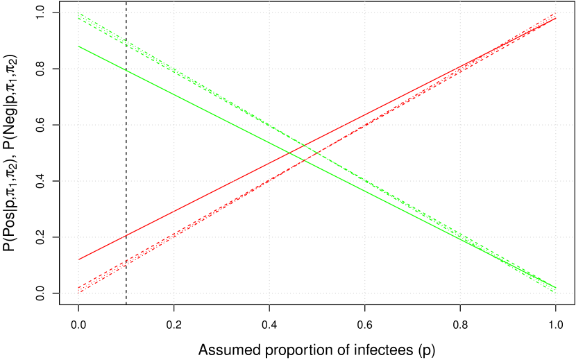
Figure 2: Probability that an individual chosen at random will result Positive (red lines with positive slope) or Negative (green lines, negative slope) as a function of the assumed proportion of infectees in the population. Solid lines for $\pi_{1}=0.98$ and $\pi_{2}=0.12$; dashed for $\pi_{1}=0.98$ and $\pi_{2}=0.02$; dotted for $\pi_{1}=0.99$ and $\pi_{2}=0.01$; dashed-dotted for $\pi_{1}=0.999$ and $\pi_{2}=0.001$.

Figure 2 shows these two probabilities as a function of $p$ for some values of $\pi_{1}$ and $\pi_{2}$.

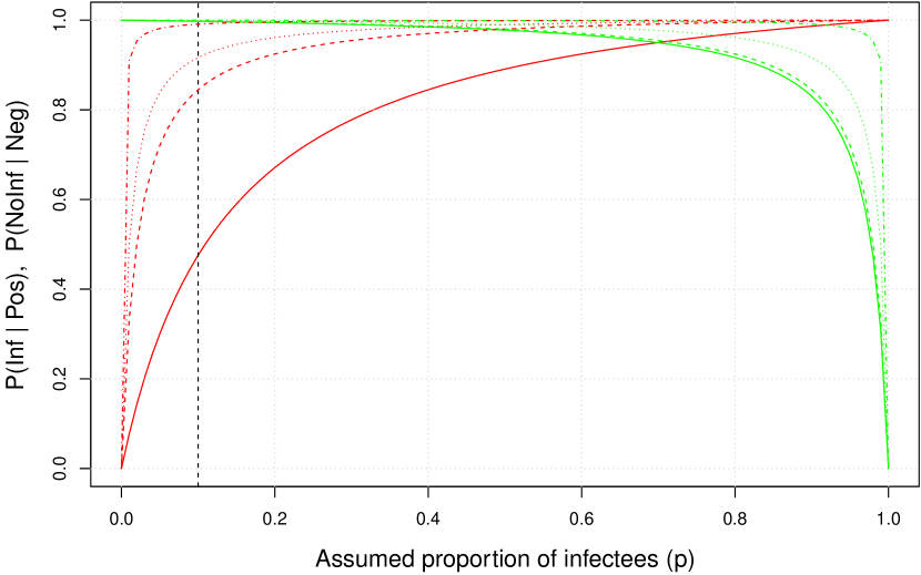
Figure 3: Probability of ‘Infected if tagged as Positive’ $[\,P(\mbox{Inf}\,|\,\mbox{Pos})$, red line, null at $p=0\,]$ and probability of ‘Not Infected if tagged as Negative’ $[\,P(\mbox{NoInf}\,|\,\mbox{Neg})$, green line, null at $p=1\,]$ as a function of $p$, calculated from Eqs. (14) and (15) for $\pi_{1}=0.98$ and $\pi_{2}=0.12$ (solid lines). For comparison, we have also included (dashed lines) the case of $\pi_{2}$ reduced to 0.02, thus increasing the ‘specificity’ to 0.98. Then there are the cases of a higher quality test $[\pi_{1}=(1-\pi_{2})=0.99]$, shown by dotted lines and of an extremely good test $[\pi_{1}=(1-\pi_{2})=0.999)]$ shown by dotted-dashed lines. (The probabilities to tag an individual, chosen at random, as positive or negative, for the same sets of parameters, were shown in Fig. 2.)

Figure 3 shows, by solid lines, $P(\mbox{Inf}\,|\,\mbox{Pos},\pi_{1},\pi_{2},p)$ and $P(\mbox{NoInf}\,|\mbox{Neg},,\pi_{1},\pi_{2},p)$ as a function of $p$, having fixed $\pi_{1}$ and $\pi_{2}$ at our nominal values 0.98 and 0.12. They are identical to those of Fig. 1, the only difference being the label of the $y$ axis, now expressed in terms of conditional probabilities. In the same figure we have also added the results obtained with other sets of parameters $\pi_{1}$ and $\pi_{2}$, as indicated directly in the figure caption.

Analyzing the above four formulae, besides the trivial ideal condition obtained by $\pi_{1}=1$ and $\pi_{2}=0$, one can make a risk analysis in order to optimize the parameters, depending on the purpose of the test. For example, we can rewrite Eq. (14) as

$$P(\mbox{Inf}\,|\,\mbox{Pos},\pi_{1},\pi_{2},p) = \frac{1}{1+\frac{\pi_{2}}{\pi_{1}}\cdot\frac{(1-p)}{p}}\,:$$ (18)

if we want to be rather sure that a Positive is really infected, then we need $\pi_{2}/\pi_{1}\ll 1$, unless $p\approx 1$. Similarly, we can rewrite Eq. (15) as

$$P(\mbox{NoInf}\,|\mbox{Neg},,\pi_{1},\pi_{2},p) = \frac{1}{1+\frac{1-\pi_{1}}{1-\pi_{2}}\cdot\frac{p}{1-p}}\,:$$

in this case, as we have learned, in order to be quite confident that the negative test implies no infection, we need $(1-\pi_{1})\ll 1$, that is, for realistic values of $\pi_{2}$, a value of $\pi_{1}$ practically equal to 1, unless $p$ is rather small, as we can see from Fig. 3. (In order to show the importance to reduce $\pi_{2}$, rather than to increase $\pi_{1}$, in the case of low proportion of infectees in the population, we show in Fig. 4 the results based on some other sets of parameters.)

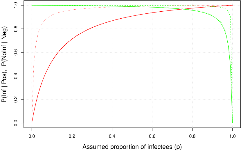
Figure 4: Same as Fig. 3, but with different parameters. Solid lines: $\pi_{1}=0.99$ and $\pi_{2}=0.10$. Dashed lines (the red one, describing $P(\mbox{Inf}\,|\,\mbox{Pos})$ overlaps perfectly with the continuous one): $\pi_{1}=0.999$ and $\pi_{2}=0.10$. Dotted lines (the green one, describing $P(\mbox{NoInf}\,|\,\mbox{Neg})$, almost overlaps the solid one): $\pi_{1}=0.99$ and $\pi_{2}=0.01$.

3.2 Initial odds, final odds and Bayes’ factor

Let us go again to the above formulae, which we rewrite in different ways in order to get some insights on what is going on. Before the test, if no other information is available, the initial odds Infected vs Not Infected are given by

$$\frac{P_{0}(\mbox{Inf})}{P_{0}(\mbox{NoInf})} = \frac{p}{1-p}\,,$$

equal to $1/9$ for our reference value of $p=0.1$. After the test has resulted in Positive the new probability of Infected is given by Eq. (8). The corresponding probability of Not Infected is given by a fraction that has the same denominator but $P(\mbox{Pos}\,|\,\mbox{NoInf})\cdot P_{0}(\mbox{NoInf})$ as numerator. The final odds are then given by

$$\frac{P(\mbox{Inf}\,|\,\mbox{Pos})}{P(\mbox{NoInf}\,|\,\mbox{Pos})} = \frac{P(\mbox{Pos}\,|\,\mbox{Inf})}{P(\mbox{Pos}\,|\,\mbox{NoInf})}\times\frac{P_{0}(\mbox{Inf})}{P_{0}(\mbox{NoInf})}\,.$$ (19)

Using our numerical values, we get

$$\frac{P(\mbox{Inf}\,|\,\mbox{Pos})}{P(\mbox{NoInf}\,|\,\mbox{Pos})} = \frac{\pi_{1}}{\pi_{2}}\times\frac{p}{1-p}$$

$$\approx 8.2\times\frac{1}{9}\,.$$

The effect of the test resulting in Positive has been to modify the initial odds by the factor

$$BF_{\mbox{\footnotesize Inf}\,vs\,\mbox{\footnotesize NoInf}}\,(\mbox{Pos})=\frac{P(\mbox{Pos}\,|\,\mbox{Inf})}{P(\mbox{Pos}\,|\,\mbox{NoInf})}\,,$$

known as Bayes’ Factor. In our case this factor is equal to $\pi_{1}/\pi_{2}\approx 8.2$. This means that after a person has been tagged as Positive, the odds Infected vs Not Infected have increased by this factor. But since the initial odds were $1/9$, the final odds are just below 1, that is about 1-to-1, or 50-50.

In the same way we can define the Bayes Factor Not Infected vs Infected in the case of a negative result:

$$BF_{\mbox{\footnotesize NoInf}\,vs\,\mbox{\footnotesize Inf}}\,(\mbox{Neg}) = \frac{P(\mbox{Neg}\,|\,\mbox{NoInf})}{P(\mbox{Neg}\,|\,\mbox{Inf})}=\frac{1-\pi_{2}}{1-\pi_{1}}=44$$

This is the reason why, for a hypothetical proportion of infectees in the population of $10\%$, a negative result makes one practically sure to be not infected. The initial odds of 9-to-1 are multiplied by a factor 44, thus reaching 396, about 400-to-1, resulting into a probability of not being infected of 396/397, or 99.75%.

3.3 What do we learn by a second test?

Let us imagine that the same individual undergoes a second test and that the result is again Positive. How should we update our believes that this individual is infected, in the light of the second observation? The first idea would be to apply Bayes’ rule in sequence, thus getting an overall Bayes’ Factor of $(\pi_{1}/\pi_{2})^{2}\approx 67$ that, multiplied by the initial odds of $1/9$, would give posterior odds of 7.4, or a probability of being infected of 88%, still far from a practical certainty. But the real question is if we can apply twice the same kind of test to the same person. It is easy to understand that the multiplication of the Bayes’ factors assumes (stochastic) independence among them. In fact, according to probability theory we have to replace now Eq. (19) by

$$\frac{P(\mbox{Inf}\,|\,\mbox{Pos}^{(1)},\mbox{Pos}^{(2)})}{P(\mbox{NoInf}\,|\,\mbox{Pos}^{(1)},\mbox{Pos}^{(2)})} = \frac{P(\mbox{Pos}^{(1)},\mbox{Pos}^{(2)}\,|\,\mbox{Inf})}{P(\mbox{Pos}^{(1)},\mbox{Pos}^{(2)}\,|\,\mbox{NoInf})}\times\frac{P_{0}(\mbox{Inf})}{P_{0}(\mbox{NoInf})}\,,$$ (20)

having indicated by $\mbox{Pos}^{(1)}$ and $\mbox{Pos}^{(2)}$ the two outcomes. Numerator and denominator of the Bayes’ Factor are then

$$P(\mbox{Pos}^{(1)},\mbox{Pos}^{(2)}\,|\,\mbox{Inf}) = P(\mbox{Pos}^{(2)}\,|\,\mbox{Pos}^{(1)},\mbox{Inf})\cdot P(\mbox{Pos}^{(1)}\,|\,\mbox{Inf})$$

$$P(\mbox{Pos}^{(1)},\mbox{Pos}^{(2)}\,|\,\mbox{NoInf}) = P(\mbox{Pos}^{(2)}\,|\,\mbox{Pos}^{(1)},\mbox{NoInf})\cdot P(\mbox{Pos}^{(1)}\,|\,\mbox{NoInf})\,,$$

which can be rewritten as

$$P(\mbox{Pos}^{(1)},\mbox{Pos}^{(2)}\,|\,\mbox{Inf}) = P(\mbox{Pos}^{(2)}\,|\,\mbox{Inf})\cdot P(\mbox{Pos}^{(1)}\,|\,\mbox{Inf})$$

$$P(\mbox{Pos}^{(1)},\mbox{Pos}^{(2)}\,|\,\mbox{NoInf}) = P(\mbox{Pos}^{(2)}\,|\,\mbox{NoInf})\cdot P(\mbox{Pos}^{(1)}\,|\,\mbox{NoInf})\,,$$

and therefore we can factorize the two Bayes’ factors, only if the two test results are independent. But this is far from being obvious. If the test response depends on something one has in the blood, different from the virus one is searching for, a second test of the same kind will most likely give the same result.

4 Uncertainty about $\pi_{1}$ and $\pi_{2}$

Until now we have used the nominal values of $\pi_{1}$ and $\pi_{2}$ of Ref. [2], and have already seen how our probabilistic conclusions change if other sets of values are employed. But these two model parameters come from tests performed on selected people, known with certainty to be infected or not. More precisely $\pi_{1}=0.98$ results from 400 surely infected, 392 of which resulted positive; $\pi_{2}=0.12$ from 200 surely not infected, 176 of which resulted negative [2].

4.1 From $P(n_{P_{I}}\,|\,n_{I},\pi_{1})$ to $f(\pi_{1}\,|\,n_{P_{I}},n_{I})$: Bayes’ rule applied to ‘numbers’

It is rather obvious to think that, repeating the same test with samples of exactly the same size, but involving different individuals, no one would be surprised to count different numbers of positives and negatives in the two samples. In fact, sticking for a while only to infectees and assuming an exact value of $\pi_{1}$, the number $n_{P_{I}}$ of positives is given by the binomial distribution,

$$f(n_{P_{I}}\,|\,n_{I},\pi_{1})\equiv P(n_{P_{I}}\,|\,n_{I},\pi_{1}) = \frac{n_{I}!}{n_{P_{I}}!\cdot(n_{I}-n_{P_{I}})!}\cdot\pi_{1}^{n_{P_{I}}}\cdot(1-\pi_{1})^{n_{I}-n_{P_{I}}}\,,\ \ \ \$$ (21)

that is, in short (with ‘$\sim$’ to be read as ‘follows…’),

$$n_{P_{I}} \sim \mbox{Binom}(n_{I},\pi_{1}).$$

The probability distribution (21) describes how much we have to rationally believe to observe the possible values of $n_{P_{I}}$ (integers between 0 and $n_{I}$), given $n_{I}$ and $\pi_{1}$.

An inverse problem is to infer $\pi_{1}$, given $n_{I}$ and the observed number $n_{P_{I}}$ (indeed, there is also a second inverse problem, that is inferring $n_{I}$ from $n_{P_{I}}$ and $\pi_{1}$ – the three problems are represented graphically by the networks of Fig. 5).

Figure 5: Graphical models of the binomial distribution (left) and its ‘inverse problems’. The symbol ‘$\surd$’ indicates the ‘observed’ nodes of the network, that is the value of the quantity associated to it is (assumed to be) certain. The other node (only one in this simple case) is ‘unobserved’ and it is associated to a quantity whose value is uncertain.

This is the kind of Problem in the Doctrine of Chances first solved by Bayes [21], and, independently and in a more refined way, by Laplace [13] about 250 years ago. Applying the result of probability theory that nowadays goes under the name of Bayes’ theorem (or Bayes’ rule) that we have introduced in the previous section, we get, apart from the normalization factor $[$hereafter the same generic symbol is used for both probability functions and probability density functions (pdf), being the meaning clear from the context$]$:

$$f(\pi_{1}\,|\,n_{P_{I}},n_{I}) \propto f(n_{P_{I}}\,|\,\pi_{1},n_{I})\cdot f_{0}(\pi_{1})$$ (22)

$$\propto \pi_{1}^{n_{P_{I}}}\cdot(1-\pi_{1})^{n_{I}-n_{P_{I}}}\cdot f_{0}(\pi_{1})\,,$$ (23)

where $f_{0}(\pi_{1})$ is the prior pdf, that describes how we believe in the possible values of $\pi_{1}$ ‘before’ (see footnote 11 and Sec. 8.7) we get the knowledge of the experiment resulting into $n_{P_{I}}$ successes in $n_{I}$ trials. Naively one could say that all possible values of $\pi_{1}$ are equally possible, thus resulting in $f_{0}(\pi_{1})=1$. But this is absolutely unreasonable, in the case of instrumentation and procedures devised by experts in order to hopefully tag infected people as positive. Therefore the value of $\pi_{1}$ should be most likely in the region above $\approx 90\%$, though without sharp cut below it. Similarly, reasonable values of $\pi_{2}$ are expected to be in the region below $\approx 10\%$.

4.2 Conjugate priors

At this point, remembering Laplace’s dictum that “probability is good sense reduced to a calculus”, we need to model the prior in a reasonable but mathematically convenient way. A good compromise for this kind of problem is the Beta probability function, which we remind here, written for the generic variable $x$ and neglecting multiplicative factors in order to focus, at this point, on its structure:

$$f(x\,|\,r,s) \propto x^{r-1}\cdot(1-x)^{s-1}\hskip 17.07182pt\left\{\!\begin{array}[]{l}r,\,s>0\\ 0\leq x\leq 1\,.\end{array}\right.$$ (26)

We see that for $r=s=1$ a uniform distribution is recovered. An important remark is that for $r>1$ the pdf vanishes at $x=0$; for $s>1$ it vanishes at $x=1$. It follows that, if $r$ and $s$ are both above 1, we can see at a glance that the function has a single maximum. It is easy to calculate that it occurs at (‘modal value’)

$$x_{m} = \frac{r-1}{r+s-2}\,.$$ (27)

Expected value and variance ($\sigma^{2}$) are

$$\mu=\mbox{E}(X) = \frac{r}{r+s}$$ (28)

$$\sigma^{2}=\mbox{Var}(X) = \frac{r\cdot s}{(r+s+1)\cdot(r+s)^{2}}\,.$$ (29)

In the case of uniform distribution, recovered by $r=s=1$, we obtain the well known $\mbox{E}(X)=1/2$ and $\sigma(X)=1/\sqrt{12}$ (and, obviously, there is no single modal value). For large $r=s$, we get $\sigma(X)\approx 1/\sqrt{8\,r}$: as the values of $r$ and $s$ increases, the distribution becomes very narrow around $1/2$.

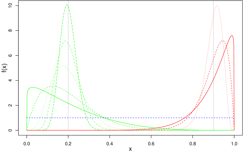
Figure 6: Examples of Beta distributions. The curves preferring small values of the generic variable $x$, all having $\mbox{E}(X)=0.2$ are obtained with (widest to narrowest) $r=1.1,\,2,\,5,\,10$ and $s=4\,r$ ($\sigma$: 0.16, 0.12, 0.078, 0.056). Those preferring larger values of $x$, all having $\mbox{E}(X)=0.9$ are obtained with (again widest to narrowest) $s=1.1,\,2,\,5$ and $r=9\,s$ ($\sigma$: 0.087, 0.065, 0.042).

Examples, with values of $r$ and $s$ to possibly model the priors we are interested in, are shown in Fig. 6.

Using the Beta distribution for $f_{0}(\pi_{1})$, our inferential problem is promptly solved, since Eq. (23) becomes, besides a normalization factor and with parameters indicated as $r_{0}$ and $s_{0}$ in order to remind their role of prior parameters,

$$f(\pi_{1}\,|\,n_{I},n_{P_{I}},r_{0},s_{0}) \propto \pi_{1}^{n_{P_{I}}}\cdot(1-\pi_{1})^{n_{I}-n_{P_{I}}}\cdot\pi_{1}^{r_{0}-1}\,(1-\pi_{1})^{s_{0}-1}$$ (30)

$$\propto \pi_{1}^{n_{P_{I}}+r_{0}-1}\cdot(1-\pi_{1})^{(n_{I}-n_{P_{I}})+s_{0}-1}$$ (31)

So, the posterior is still a Beta distribution, with parameters updated according to the simple rules

$$r_{f} = r_{0}+n_{P_{I}}$$ (32)

$$s_{f} = s_{0}+(n_{I}-n_{P_{I}})\,.$$ (33)

For this reason the Beta is known to be the prior conjugate of the binomial distribution. In terms of our variables,

$$n_{P_{I}}\sim\mbox{Binom}(n_{I},\pi_{1}) \Longrightarrow \pi_{1}\sim\mbox{Beta}(r_{0}+n_{P_{I}},s_{0}+n_{I}-n_{P_{I}})\,.$$ (34)

The advantage of using the Beta prior conjugate is self-evident, if we can choose values of $r_{0}$ and $s_{0}$ that reasonably model our prior belief about $\pi_{1}$. For this reason it might be useful to invert Eq. (28) and (29), thus getting

$$r_{0} = \frac{(1-\mu_{0})\cdot\mu_{0}^{2}}{\sigma_{0}^{2}}-\mu_{0}$$ (35)

$$s_{0} = \frac{1-\mu_{0}}{\mu_{0}}\cdot r_{0}\,.$$ (36)

So, for example, if we think that $\pi_{1}$ should be around 0.95 with a standard uncertainty of about $0.05$, we get then $r_{0}=17.1$ and $s_{0}=0.9$, the latter slightly increased ‘by hand’ to $s_{0}=1.1$ because our rational prior has to assign zero probability to $\pi_{1}=1$, that would imply the possibility of a perfect test. The experimental data update then $r$ and $s$ to $r=409.1$ and $s=9.1$. For $\pi_{2}$ we model a symmetric prior, with expected value 0.05 and $\sigma=0.05$. We just need to swap $r$ and $s$, thus getting $r_{0}=1.1$ and $s_{0}=17.1$, updated by the data to $r=25.1$ and $s=193.1$. The results are shown in Fig. 7.

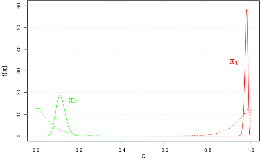
Figure 7: Priors (dashed) and posterior (solid) probability density functions of $\pi_{1}$ and $\pi_{2}$.

Expressed in terms of expected value $\pm$ standard deviation they are

$$\pi_{1} = 0.978\pm 0.007$$ (37)

$$\pi_{2} = 0.115\pm 0.022\,.$$ (38)

As we can easily guess, using simply 0.98 and 0.12, as we have done in the previous sections, will give essentially the same results, in terms of expectations. Anyway, in order to be internally consistent hereafter our reference values will be $\pi_{1}=0.978$ and $\pi_{2}=0.115$.

4.3 Expected value or most probable value of $\pi_{1}$ and $\pi_{2}$?

At this point someone would object that one should use the most probable values of $\pi_{1}$ and $\pi_{2}$, rather than their expected values. The answer is rather simple. Let us consider again Eq. (10). Assuming a well precise value of $\pi_{1}$, the probability of Positive if Infected is exactly equal to $\pi_{1}$. However, if we want to evaluate $P(\mbox{Pos}\,|\,\mbox{Inf})$, taking into account all possible values of $\pi_{1}$ and how much we believe each of them, that is $f(\pi_{1})$, we just to need to use a well known result of probability theory:

$$P(\mbox{Pos}\,|\,\mbox{Inf}) = \int_{0}^{1}\!P(\mbox{Pos}\,|\,\mbox{Inf},\pi_{1})\cdot f(\pi_{1})\,\mbox{d}\pi_{1}\,.$$ (39)

But, being $P(\mbox{Pos}\,|\,\mbox{Inf},\pi_{1})=\pi_{1}$, we get

$$P(\mbox{Pos}\,|\,\mbox{Inf}) = \int_{0}^{1}\!\pi_{1}\cdot f(\pi_{1})\,\mbox{d}\pi_{1}\,,$$ (40)

in which we recognize the expected value of $\pi_{1}$.

4.4 Effect of the uncertainties on $\pi_{1}$ and $\pi_{2}$ on the probabilities of interest

The immediate question that follows is how the uncertainties concerning these two parameters change the probabilities of interest. We start reporting in Tab. 1

	$p$
Probabilities
	$0.01$	$0.05$	$0.10$	$0.15$	$0.20$	$0.50$
$P(\mbox{Inf}\,|\,\mbox{Pos},\pi_{1}\!=\!0.98,\pi_{2}\!=\!0.12,p)$	0.0762	0.301	0.476	0.590	0.671	0.891
$P(\mbox{NoInf}\,|\,\mbox{Neg},\pi_{1}\!=\!0.98,\pi_{2}\!=\!0.12,p)$	0.9998	0.999	0.997	0.996	0.994	0.978
$P(\mbox{Inf}\,|\,\mbox{Pos},\mbox{\boldmath$\pi_{1}=0.978,\pi_{2}=0.115$},p)$	$0.0791$	$0.309$	$0.486$	$0.600$	$0.680$	$0.895$
$P(\mbox{NoInf}\,|\,\mbox{Neg},\mbox{\boldmath$\pi_{1}=0.978,\pi_{2}=0.115$},p)$	$0.9997$	$0.999$	$0.997$	$0.996$	$0.994$	$0.976$
$P(\mbox{Inf}\,|\,\mbox{Pos},\pi_{1}\!=\!0.985,\pi_{2}\!=\!0.115,p)$	0.0796	0.311	0.488	0.602	0.682	0.895
$P(\mbox{NoInf}\,|\,\mbox{Neg},\pi_{1}\!=\!0.985,\pi_{2}\!=\!0.115,p)$	0.9998	0.999	0.998	0.997	0.996	0.983
$P(\mbox{Inf}\,|\,\mbox{Pos},\pi_{1}=0.971,\pi_{2}=0.115,p)$	0.0786	0.308	0.484	0.598	0.679	0.894
$P(\mbox{NoInf}\,|\,\mbox{Neg},\pi_{1}=0.971,\pi_{2}=0.115,p)$	0.9998	0.998	0.996	0.994	0.992	0.968
$P(\mbox{Inf}\,|\,\mbox{Pos},\pi_{1}\!=\!0.978,\pi_{2}\!=\!0.137,p)$	0.0673	0.273	0.442	0.557	0.641	0.877
$P(\mbox{NoInf}\,|\,\mbox{Neg},\pi_{1}\!=\!0.978,\pi_{2}\!=\!0.137,p)$	0.9997	0.999	0.997	0.996	0.994	0.975
$P(\mbox{Inf}\,|\,\mbox{Pos},\pi_{1}=0.978,\pi_{2}=0.093,p)$	0.0960	0.356	0.539	0.650	0.724	0.913
$P(\mbox{NoInf}\,|\,\mbox{Neg},\pi_{1}=0.978,\pi_{2}=0.093,p)$	0.9998	0.999	0.997	0.996	0.994	0.976
$P(\mbox{Inf}\,|\,\mbox{Pos},\pi_{1}=0.985,\pi_{2}=0.093,p)$	0.0966	0.358	0.541	0.651	0.726	0.914
$P(\mbox{NoInf}\,|\,\mbox{Neg},\pi_{1}=0.985,\pi_{2}=0.093,p)$	0.9998	0.999	0.998	0.997	0.996	0.984
$P(\mbox{Inf}\,|\,\mbox{Pos},\pi_{1}=0.971,\pi_{2}=0.137,p)$	0.0668	0.272	0.441	0.556	0.639	0.876
$P(\mbox{NoInf}\,|\,\mbox{Neg},\pi_{1}=0.971,\pi_{2}=0.137,p)$	0.9997	0.998	0.996	0.994	0.992	0.967
$P(\mbox{Inf}\,|\,\mbox{Pos},\pi_{1}=0.985,\pi_{2}=0.137,p)$	0.0677	0.275	0.444	0.559	0.643	0.878
$P(\mbox{NoInf}\,|\,\mbox{Neg},\pi_{1}=0.985,\pi_{2}=0.137,p)$	0.9998	0.999	0.998	0.997	0.996	0.983
$P(\mbox{Inf}\,|\,\mbox{Pos},\pi_{1}=0.971,\pi_{2}=0.093,p)$	0.0954	0.355	0.537	0.648	0.723	0.913
$P(\mbox{NoInf}\,|\,\mbox{Neg},\pi_{1}=0.971,\pi_{2}=0.093,p)$	0.9997	0.998	0.996	0.994	0.992	0.969
$P(\mbox{Inf}\,|\,\mbox{Pos},\mbox{\boldmath$p$})$	0.0815	0.314	0.490	0.603	0.682	0.895
$P(\mbox{NoInf}\,|\,\mbox{Neg},\mbox{\boldmath$p$})$	0.9998	0.999	0.997	0.996	0.994	0.976

Table 1: Probability of Infected and Not Infected, given the test result, as a function of the model parameters. The third and fourth rows, in boldface, are for our reference values of $\pi_{1}$ and $\pi_{2}$. The last two rows are the results ‘integrating over’ all the possibilities of $\pi_{1}$ and $\pi_{2}$, according to Eq. (41) and (42), with the integrals done in practice by Monte Carlo sampling.

the dependence of $P(\mbox{Inf}\,|\,\mbox{Pos},\pi_{1},\pi_{2},p)$ and $P(\mbox{NoInf}\,|\,\mbox{Neg},\pi_{1}\pi_{2},p)$, on which we particularly focused in the previous sections, on the three parameters. The dependence on $p$ is shown in the different columns, while the sets of $\pi_{1}$ and $\pi_{2}$ are written explicitly in the conditionands of the different probabilities. We start from the nominal values of 0.98 and 0.12 taken from Ref. [2] (first two rows of the table). Then we use the expected values calculated in the previous section (third and fourth rows, in boldface), followed by variations of $\pi_{1}$ and $\pi_{2}$ based on $\pm$ one standard deviation from their expected values.

We see that the probabilities of interest do not change significantly, the main effect being due to the assumed proportion of infectees in the population. One could argue that the dependence on $\pi_{1}$ and $\pi_{2}$ could be larger, if larger deviations of the parameters were considered. Obviously this is true, but one has to take also into account the (small) probabilities of large deviations from the mean values, especially if we allow simultaneous deviations of both parameters.

A more relevant question is, instead, how do $P(\mbox{Inf}\,|\,\mbox{Pos})$ and $P(\mbox{NoInf}\,|\,\mbox{Neg}$) change, if we take into account all possible variations of the two parameters (weighed by their probabilities!). This is easily done, applying the result of probability theory that we have already used above. We get, for the probabilities we are mostly interested in,

$$P(\mbox{Inf}\,|\,\mbox{Pos},p) = \int_{0}^{1}\!\!\int_{0}^{1}\!P(\mbox{Inf}\,|\,\mbox{Pos},\pi_{1},\pi_{2},p)\cdot f(\pi_{1},\pi_{2})\,\mbox{d}\pi_{1}\mbox{d}\pi_{2}\,.$$ (41)

$$P(\mbox{NoInf}\,|\,\mbox{Neg},p) = \int_{0}^{1}\!\!\int_{0}^{1}\!P(\mbox{NoInf}\,|\,\mbox{Neg},\pi_{1},\pi_{2},p)\cdot f(\pi_{1},\pi_{2})\,\mbox{d}\pi_{1}\mbox{d}\pi_{2}\,,$$ (42)

where $f(\pi_{1},\pi_{2})$ can be factorized into $f(\pi_{1})\cdot f(\pi_{2})$. The integral can be easily done by Monte Carlo, whose implementation in the R language [11], both for $P(\mbox{Inf}\,|\,\mbox{Pos})$ and $P(\mbox{NoInf}\,|\,\mbox{Neg})$, is given in Appendix B.1.

We get, for our arbitrary reference value of $p=0.1$, $P(\mbox{Inf}\,|\,\mbox{Pos},p=0.1)=0.49038$ and $P(\mbox{NoInf}\,|\,\mbox{Neg},p=0.1)=0.99727$, to be compared to 0.4858 and 0.9973, respectively, if the expected values were used. The results, shown with an exaggerated number of digits just to appreciate tiny differences, are practically the same. This result could sound counter-intuitive, especially if one thinks that $\pi_{2}$ has an almost 20% intrinsic standard uncertainty. The reason is due to the fact that the dependence of the probabilities of interest on $\pi_{1}$ and $\pi_{2}$ is rather linear in the region where their probability mass is concentrated, as shown in Fig. 8.

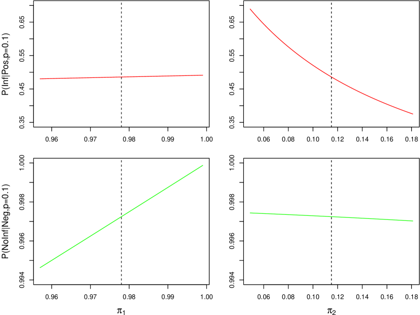
Figure 8: Dependence of $P(\mbox{Inf}\,|\,\mbox{Pos})$ (upper plots) and $P(\mbox{NoInf}\,|\,\mbox{Neg})$ (lower plots) on $\pi_{1}$ (left hand plots, for $\pi_{2}=0.115$ and $p=0.1$) and on $\pi_{2}$ (right hand plots, for $\pi_{1}=0.978$ and $p=0.1$). The parameters $\pi_{1}$ and $\pi_{2}$ are allowed to change withing a range of $\pm 3\,\sigma$’s around their expected values.

This rather good linearity causes a high degree of cancellations in the integral. This explains why the only perceptible effect appears in $P(\mbox{Inf}\,|\,\mbox{Pos},p=0.1)$, slightly larger than the number calculated at the expected values (49.04% vs 48.58%), caused by the small non-linearity of that probability as a function of $\pi_{2}$, as shown in the upper, right hand plot of Fig. 8: symmetric variations of $\pi_{2}$ cause slightly asymmetric variations of $P(\mbox{Inf}\,|\,\mbox{Pos},p=0.1)$, thus slightly favoring higher values of that probability.

4.5 Adding also the uncertainty about $p$

Now that we have learned the game, we can use it to include also the uncertainty concerning $p$. At a given stage of the pandemic we could have good reasons to guess a proportion of infected around 10%, as we have been done till now, with a sizable uncertainty, for example 5% (i.e. $p=0.10\pm 0.05$). We model, also in this case, $f(p)$ with a Beta distribution, getting $r=3.5$ and $s=31.5$. Equation (41) becomes then

$$P(\mbox{Inf}\,|\,\mbox{Pos})\! = \!\int_{0}^{1}\!\!\int_{0}^{1}\!\!\int_{0}^{1}\!P(\mbox{Inf}\,|\,\mbox{Pos},\pi_{1},\pi_{2},p)\cdot f(\pi_{1},\pi_{2},p)\,\mbox{d}\pi_{1}\mbox{d}\pi_{2}\mbox{d}p$$ (43)

$$= \!\int_{0}^{1}\!\!\int_{0}^{1}\!\!\int_{0}^{1}\!P(\mbox{Inf}\,|\,\mbox{Pos},\pi_{1},\pi_{2},p)\cdot f(\pi_{1})\cdot f(\pi_{2})\cdot f(p)\,\mbox{d}\pi_{1}\mbox{d}\pi_{2}\mbox{d}p\,,\ \ \ \ \$$ (44)

in which we have made explicit that the joint pdf factorizes, considering $\pi_{1}$, $\pi_{2}$ and $p$ independent. With a minor modification to the script provided in Appendix B.1 we get $P(\mbox{Inf}\,|\,\mbox{Pos})=0.4626$ and $P(\mbox{NoInf}\,|\,\mbox{Neg})=0.9972$, reported again with an exaggerated number of digits. We only note a small effect in $P(\mbox{Inf}\,|\,\mbox{Pos})$. As a further exercise, let also take into account $p=0.20\pm 0.10$, modeled by a $\mbox{Beta}(r\!=\!3,s\!=\!12)$. In this case the Monte Carlo integration yields $P(\mbox{Inf}\,|\,\mbox{Pos})=0.641$ and $P(\mbox{NoInf}\,|\,\mbox{Neg})=0.993$, to be compared with 0.682 and 0.994 of Tab. 1.

4.6 Uncertainty about $P(\mbox{Inf}\,|\,\mbox{Pos})$ and $P(\mbox{NoInf}\,|\,\mbox{Neg})$?

As we have seen, the probabilities of interest, taking into account all the possibilities of $\pi_{1}$, $\pi_{2}$ and $p$ are obtained as weighted averages, with weights equal to $f(\pi_{1},\pi_{2},p)$. One could then be tempted to evaluate the standard deviation too, attributing to it the meaning of ‘standard uncertainty’ about $P(\mbox{Inf}\,|\,\mbox{Pos})$ and $P(\mbox{NoInf}\,|\,\mbox{Neg})$. But some care is needed. In fact, although is quite obvious that, sticking again to $P(\mbox{Inf}\,|\,\mbox{Pos})$, we can form an idea about the variability of $P(\mbox{Inf}\,|\,\mbox{Pos},\pi_{1},\pi_{2},p)$ varying $\pi_{1}$, $\pi_{2}$ and $p$ according to $f(\pi_{1},\pi_{2},p)$ (something like we have done in Tab. 1, although we have not associated probabilities to the different entries of the table), one has to be careful in making a further step. The fact that the weighted average is $P(\mbox{Inf}\,|\,\mbox{Pos})$ comes from the rules of probability theory, namely from Eq. (43), but there is not an equivalent rule to evaluate the uncertainty of $P(\mbox{Inf}\,|\,\mbox{Pos})$.

In order to simplify the notation, let us indicate in the following lines $P(\mbox{Inf}\,|\,\mbox{Pos})$ by $\cal P$. In order to speak about standard uncertainty of $\cal P$, we first need to define the pdf $f(\cal P)$, and then evaluate average and standard deviation. But Eq. (43) does not provide that, but only a single number, that is $\cal P$ itself.

Let us reword what we just stated using a simple example. Given the ‘random variable’ $X$ and the pdf associated to it $f(x)$, mean and standard deviation of $f(x)$ provide expected value (‘$\mu_{X}$’) and standard deviation of $X$, and not of $\mu$.

5 Predicting the number of positives resulting from testing a sample

The previous sections have been dedicated to the evaluation of the probability that a particular individual, tagged as positive in a test, is really infected. In those sections we have understood how, in absence of any other hints, it is important to know the percentage $p$ of infectees in the population. Knowing this parameter is paramount also for better designing a containing strategy in addressing the pandemic. Therefore we move now to the related, but quite different problem: ‘counting’, although not in an exact way, the number of infected individuals in a population. Given the didactic spirit of this paper, we keep proceeding step-by-step. First we focus on the number of positives that we expect to observe if we check a sample using the quite imperfect test we are considering. Then we also take into account the effect of sampling a population, since, as it is rather obvious, the proportion of infected in a sample of size $n_{s}$ will not be exactly equal to that in the whole population of $N$ individuals. For this reason we distinguish, hereafter, $p_{s}$ of the sample from $p$ of the population.

5.1 Expected number of positives and its standard uncertainty

In Sec. 2.2 we have considered the numbers of positives and negatives that we expect to observe, analyzing 10000 individuals, using our initial parameters ($p_{s}=0.10$, $\pi_{1}=0.98$, $\pi_{2}=0.12$) but without taking into account the unavoidable ‘statistical fluctuation’. We do it now, using the probabilistic graphical model shown in Fig. 9,

Figure 9: Graphical model in which the number of positives could come from infected or not infected individuals. Arrows with dashed lines stand for a deterministic link, being $n_{P}$ simply equal to the sum of $n_{P_{I}}$ and $n_{P_{NI}}$.

obtained by doubling the basic one of Fig. 5, one branch for the infectees and a second for the others. Then the numbers of positives resulting from the two contributions are added up. Note in Fig. 9 the dashed arrows from the nodes $n_{P_{I}}$ and $n_{P_{NI}}$ to the node $n_{P}$: they indicate a deterministic link, being $n_{P}=n_{P_{I}}+n_{P_{NI}}$.

The probability distribution of $n_{P}$ is with good approximation Gaussian, due to the well known large numbers behavior of the binomial distribution (and, moreover, to the properties of the sum of ‘random variables’). On the other hand, the expected value and the standard deviation of $n_{P}$ can been calculated exactly, using the properties of expected values and variances, thus getting (summarizing for sake of space with the symbol $I$, staying for all available information, the conditions on which the various quantities depend):

$$\mbox{E}(n_{P}\,|\,I) = \mbox{E}(n_{P_{I}}\,|\,I)+\mbox{E}(n_{P_{NI}}\,|\,I)$$ (45)

$$= \pi_{1}\cdot n_{I}+\pi_{2}\cdot n_{NI}$$

$$= \pi_{1}\cdot p_{s}\cdot n_{s}+\pi_{2}\cdot(1-p_{s})\cdot n_{s}$$

$$\sigma^{2}(n_{P}\,|\,I) = \sigma^{2}(n_{P_{I}})+\sigma^{2}(n_{P_{I}})$$ (46)

$$= \pi_{1}\cdot(1-\pi_{1})\cdot p_{s}\cdot n_{s}+\pi_{2}\cdot(1-\pi_{2})\cdot(1-p_{s})\cdot n_{s}$$

$$\sigma(n_{P}\,|\,I) = \sqrt{\pi_{1}\cdot(1-\pi_{1})\cdot p_{s}\cdot n_{s}+\pi_{2}\cdot(1-\pi_{2})\cdot(1-p_{s})\cdot n_{s}}\,,$$ (47)

with $n_{s}$ the sample size. Expected value and standard deviation of the fraction of the number of individuals tagged as positive ($f_{P}=n_{P}/n_{s}$) are then

$$\mbox{E}(f_{P}\,|\,I)=\frac{\mbox{E}(n_{P}\,|\,I)}{n_{s}} = \pi_{1}\cdot p_{s}+\pi_{2}\cdot(1-p_{s})$$ (48)

$$\sigma(f_{P}\,|\,I)=\frac{\sigma(n_{P}\,|\,I)}{n_{s}} = \sqrt{\frac{\,\pi_{1}\cdot(1-\pi_{1})\cdot p_{s}+\pi_{2}\cdot(1-\pi_{2})\cdot(1-p_{s})\,}{\,n_{s}}}.\ \ \ \ \$$ (49)

For example, making use of our reference numbers ($n_{s}=10000$, $\pi_{1}=0.978$ and $\pi_{2}=0.115$) we get for some values of $p_{s}$ (expected value $\pm$ standard uncertainty):

$$\left.n_{P}\right|_{(n_{s}=10000,\,\pi_{1}=0.978,\,\pi_{2}=0.115,\,{\footnotesize\mbox{\boldmath$p_{s}=0.0$}})} = 1150\pm 32\ \ \ \longrightarrow\,f_{P}=0.1150\pm 0.0032$$

$$\left.n_{P}\right|_{(n_{s}=10000,\,\pi_{1}=0.978,\,\pi_{2}=0.115,\,{\footnotesize\mbox{\boldmath$p_{s}=0.1$}})} = 2013\pm 31\ \ \ \longrightarrow\,f_{P}=0.2013\pm 0.0031$$

$$\left.n_{P}\right|_{(n_{s}=10000,\,\pi_{1}=0.978,\,\pi_{2}=0.115,\,{\footnotesize\mbox{\boldmath$p_{s}=0.2$}})} = 2876\pm 29\ \ \ \longrightarrow\,f_{P}=0.2876\pm 0.0029$$

$$\left.n_{P}\right|_{(n_{s}=10000,\,\pi_{1}=0.978,\,\pi_{2}=0.115,\,{\footnotesize\mbox{\boldmath$p_{s}=0.5$}})} = 5465\pm 25\ \ \ \longrightarrow\,f_{P}=0.5465\pm 0.0025\,.$$

From this numbers we can get an idea about the precision we could get on $p_{s}$, if $\pi_{1}$ and $\pi_{2}$ were perfectly known, although their values are rather far from what one would ideally desire. For example, since under the hypotheses $p_{s}=0.1$ and $p_{s}=0$ (and similar numbers are obtained varying $p_{s}$ from $0.1$ to $0.2$) the expected difference of positives is $\Delta_{n_{P}}=863\pm 45$, it follows that, varying $p_{s}$ by $\pm 0.01$ the expected number of positives would vary by $\approx\pm\,(86\pm 4.5)$. This means that, roughly speaking, it could be possible to estimate $p_{s}$ with an uncertainty of $\pm 0.01$ or better.

Before taking into account the effects due to the uncertainties of $\pi_{1}$ and $\pi_{2}$, let us also see how the quality of the measurement depends on the sample size. In order to do this, we fix this time $p_{s}$ to our arbitrary value of $0.1$ and vary the sample size by about half order of magnitude (that is $\approx 10^{k/2}$, with $k=6,7,\ldots,10$), reporting in this case directly the expected fraction of positives:

$$\left.f_{P}\right|_{({\footnotesize\mbox{\boldmath$n_{s}=1000$}},\,\pi_{1}=0.978,\,\pi_{2}=0.115,\,p_{s}=0.1)} = 0.2013\pm 0.0097$$

$$\left.f_{P}\right|_{({\footnotesize\mbox{\boldmath$n_{s}=3000$}},\,\pi_{1}=0.978,\,\pi_{2}=0.115,\,p_{s}=0.1)} = 0.2013\pm 0.0056$$

$$\left.f_{P}\right|_{({\footnotesize\mbox{\boldmath$n_{s}=10000$}},\,\pi_{1}=0.978,\,\pi_{2}=0.115,\,p_{s}=0.1)} = 0.2013\pm 0.0031$$

$$\left.f_{P}\right|_{({\footnotesize\mbox{\boldmath$n_{s}=30000$}},\,\pi_{1}=0.978,\,\pi_{2}=0.115,\,p_{s}=0.1)} = 0.2013\pm 0.0018$$

$$\left.f_{P}\right|_{({\footnotesize\mbox{\boldmath$n_{s}=100000$}},\,\pi_{1}=0.978,\,\pi_{2}=0.115,\,p_{s}=0.1)} = 0.2013\pm 0.0010\,.$$

As we can see, if we knew perfectly $\pi_{1}$ and $\pi_{2}$, already a sample of a few thousands individuals would allow us to predict the fraction of tagged positives with a relative uncertainty of a few percent. However there are other effects to be taken into account:

• there is uncertainty about $\pi_{1}$ and $\pi_{2}$;

• the proportion of infectees in the sample is different from that in the population (that is, in general $p_{s}$ differs from $p$);

• the inference from the observed numbers of positives to $p_{s}$, and then to $p$, has to be done using sound probabilistic inferential methods.

5.2 Taking into account the uncertainty on $\pi_{1}$ and $\pi_{2}$

As we have seen in Sec. 4.4, the way to take into account all possible values of $\pi_{1}$ and $\pi_{2}$, using the rules of probability theory, consists in evaluating the following integral

$$f(n_{P}\,|\,n_{s},p_{s}) = \int_{0}^{1}\!\!\int_{0}^{1}\!f(n_{P}\,|\,n_{s},p_{s},\pi_{1},\pi_{2})\cdot f(\pi_{1})\cdot f(\pi_{2})\,\mbox{d}\pi_{1}\mbox{d}\pi_{2}\,.$$ (50)

Before tacking the problem of how to evaluate this integral, a very important remark on how we are going to model the uncertainty about $\pi_{1}$ and $\pi_{2}$ is in order.

• When we write $f(n_{P}\,|\,n_{s},p_{s},\pi_{1},\pi_{2})$, we are assuming, trivially, the same exact values of $\pi_{1}$ and $\pi_{2}$ for all the tests performed on the $n_{s}$ individuals of the sample.

• If, instead, their value is uncertain, and we describe their uncertainty by $f(\pi_{1})$ and $f(\pi_{2})$, again it means that the same two numerical values influence the results of the $n_{s}$ tests. But we just do not know with certainty which are these values.

• In particular, associating to these two parameters the pdf’s $f(\pi_{1})$ and $f(\pi_{2})$ does not mean that $\pi_{1}$ and $\pi_{2}$ fluctuate from one test to one other. The two pdf’s only describe the uncertainty on their numerical values.

• It is however reasonable to think that, from how the ‘test devices’ are built up, each item could perform slightly differently than the other, but we shall ignore these possible test-to-test fluctuations, although they could be taken into account just extending the model.

Going back to the practical issue of evaluating the integral, we use again Monte Carlo methods, employing e.g. the R script provided in Appendix B.2, for the case of $n_{s}=10000$ and $p_{s}=0.1$. The result, shown in the bottom plot of Fig. 10,

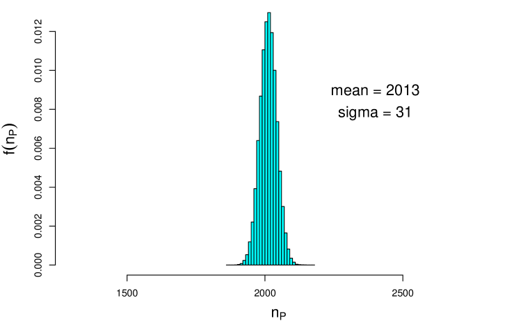
Figure 10: Probabilistic prediction of the numbers of positives, based on a hypothetical test on 10000 individuals, exactly 1000 of them being infected. In the upper plot we use $\pi_{1}=0.978$ and $\pi_{2}=0.115$. In the lower plot we take into account their possible variability (see text). The over-imposed curve shows a Gaussian with average 2013 and standard deviation 200, values obtained by the approximated Eqs. (51) and (52). (The top histogram is repeated, with enlarged horizontal scale, in Fig. 12.)

is quite impressive, compared to the top one, in which the precise values $\pi_{1}=0.978$ and $\pi_{2}=0.115$ were used. The mean of the distribution is unchanged, as more or less expected (see Sec. 4.4), but its standard deviation, which quantifies the uncertainty of the prediction, increases by more than a factor six. We have then good reasons to expect a similar effect when we will be interested in the ‘reverse’ problem, that is inferring the number of infectees in the sample from the resulting number of positives. Going into details, we see that the expected number of positives is essentially the same of Sec. 2.2 (the reduction from 2060 to 2013 is simply due to the new reference values for $\pi_{1}$ and $\pi_{2}$ we are using starting from Sec. 4). But this number is now accounted by an uncertainty, which rises to about 10% of its value, when the uncertainties about $\pi_{1}$ and $\pi_{2}$ are also taken into account.

5.2.1 Approximated formulae

Although Monte Carlo integration is a powerful tool to solve at best non trivial problems of this kind, it is very useful to get, whenever it is possible, approximate solutions in order to have an idea, analyzing the resulting formulae, of how the result depends on the assumptions. First at all, in analogy to what we have seen in Sec. 4.4, we can be rather confident that the expected value of $n_{P}$ is not significantly affected, as also confirmed by the Monte Carlo results shown in Fig. 10. The variance, given by Eq. (46) is, instead, increased by terms whose approximated values can be obtained by linearization. These are the resulting approximated expressions:

$$\mbox{E}(n_{P}) \approx \mbox{E}(\pi_{1})\cdot p_{s}\cdot n_{s}+\mbox{E}(\pi_{2})\cdot(1-p_{s})\cdot n_{s}$$ (51)

$$\sigma^{2}(n_{P}) \approx \mbox{E}(\pi_{1})\cdot(1-\mbox{E}(\pi_{1}))\cdot p_{s}\cdot n_{s}+\mbox{E}(\pi_{2})\cdot(1-\mbox{E}(\pi_{2}))\cdot(1-p_{s})\cdot n_{s}$$ (52)

$$+\,\sigma^{2}(\pi_{1})\cdot p_{s}^{2}\cdot n_{s}^{2}+\sigma^{2}(\pi_{2})\cdot(1-p_{s})^{2}\cdot n_{s}^{2}\,.$$

Applying them to the case shown in Fig. 10 we obtain an expected value of 2013 and a standard deviation of 200, in excellent agreement with the Monte Carlo result. In order to have an idea of the deviation from ‘normality’ we also over-impose, to the bottom histogram of the figure, the Gaussian having average and standard deviation calculated by Eq. (51) and (52) – we remind that the top histogram has instead strong theoretical reasons to be, with very good approximation, normally distributed (a zoomed version of the same histogram is reported in Fig. 12).

As a further check, let us see what happens in the case of no infected individuals in the sample, that is $p_{s}=0$. The Monte Carlo results are shown in Fig. 11,

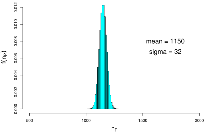
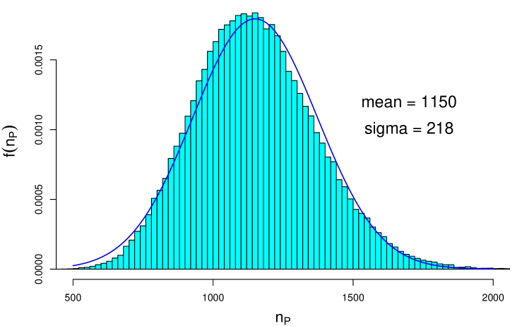
Figure 11: Same as Fig. 10, but in the case of no infected individual in the sample ($p_{s}=0$). The over-imposed Gaussian has average 1150 and standard deviation 222.

We see that, as already stated qualitatively in Sec. 2, number of positives can occur well below the value one would compute only reasoning on rough estimates (1150 in this case). Therefore, since the formulae derived in that way were unreliable, a probabilistic treatment of the problem is needed in order to take into account the fact that fluctuations around expected values do usually occur. Also in this case the approximated results obtained by Eqs. (51) and (52) are in excellent agreement with the Monte Carlo estimates, yielding $1150\pm 222$ (and, again, the Gaussian approximation is not too bad, at least within a couple of standard deviations from the mean value). The approximation remains good also for high values of $p_{s}$. For example, for the quite high value of $p_{s}=0.5$, the Monte Carlo integration gives $5465\pm 116$ versus an approximated result of $5465\pm 118$.

A natural question is how the results change not only with the proportion of infectees in the sample, but also with the size of the sample. The answer is given in Tab. 2, with $n_{s}$ varying, in steps of roughly half order of magnitude, from the ridiculous value of 100 up to 100000 (that is $\approx 10^{k/2}$, with $k=4,5,\ldots,10$).

$\mbox{\boldmath$p_{s}$}\rightarrow$	0.01	0.05	0.10	0.15	0.20	0.50
$\mbox{\boldmath$\mbox{\bf E}(f_{P})$}\rightarrow$	0.124	0.158	0.201	0.244	0.287	0.546
$n_{s}$:	standard uncertainties
100	(0.032)	(0.031)	(0.031)	(0.030)	(0.029)	(0.025)
	[0.038]	[0.037]	[0.036]	[0.035]	[0.034]	[0.027]
300	(0.018)	(0.018)	(0.018)	(0.017)	(0.017)	(0.014)
	[0.028]	[0.027]	[0.026]	[0.025]	[0.024]	[0.018]
1000	(0.010)	(0.010)	(0.010)	(0.009)	(0.009)	(0.008)
	[0.024]	[0.023]	[0.022]	[0.021]	[0.020]	[0.014]
3000	(0.006)	(0.006)	(0.006)	(0.005)	(0.005)	(0.005)
	[0.022]	[0.021]	[0.020]	[0.019]	[0.018]	[0.012]
10000	(0.003)	(0.003)	(0.003)	(0.003)	(0.003)	(0.002)
	[0.022]	[0.021]	[0.020]	[0.019]	[0.018]	[0.012]
30000	(0.002)	(0.002)	(0.002)	(0.002)	(0.002)	(0.001)
	[0.021]	[0.021]	[0.020]	[0.018]	[0.017]	[0.011]
100000	(0.001)	(0.001)	(0.001)	(0.001)	(0.001)	(0.001)
	[0.021]	[0.021]	[0.019]	[0.018]	[0.017]	[0.011]

Table 2: Predicted fraction of tagged positives in a sample ($f_{P}$) as a function of the assumed proportion of infected individuals in the sample ($p_{s}$), also taking into account the uncertainty on the test parameters $\pi_{1}$ and $\pi_{2}$ (numbers in squared brackets – those in round brackets are evaluated at the expected values of $\pi_{1}$ and $\pi_{2}$).

The chosen values of $p_{s}$ are the same of $p$ of Tab. 1. For an easier comparison, the fraction $f_{p}$ of positively tagged individual is provided. The expected value of $f_{P}$, depending essentially only on $p_{s}$, is reported in the second row of the table. Two standard uncertainties are reported for each combination of $p_{s}$ and $n_{s}$: the first, in round brackets, only takes into account the two binomial distributions (‘statistical errors’, in old style physicist’s jargon); the second, in square brackets takes into account also the possible variability of $\pi_{1}$ and $\pi_{2}$ (‘systematic error’, in the same jargon). They have all been evaluated by Monte Carlo, but the agreement with the approximated formula (52) has been checked.

5.3 General considerations on the approximated evaluation of $\sigma(n_{P})$ by Eq. (52)

At this point some further remarks on the utility of Eq. (52) is in order. Its advantage, within its limits of validity (checked in our case), is that it allows to disentangle the contributions to the overall uncertainty. In particular we can rewrite it as

$$\sigma(n_{P}) \approx \sigma_{R}(n_{P})\oplus\sigma_{\pi_{1}}(n_{P})\oplus\sigma_{\pi_{2}}(n_{P})\,,$$ (53)

that is a ‘quadratic sum’ (or ‘quadratic combination’, indicated by the symbol ‘$\oplus$’) of three contributions,

$$\sigma_{R}(n_{P}) = \sqrt{\mbox{E}(\pi_{1})\cdot(1-\mbox{E}(\pi_{1}))\cdot p_{s}\cdot n_{s}+\mbox{E}(\pi_{2})\cdot(1-\mbox{E}(\pi_{2}))\cdot(1-p_{s})\cdot n_{s}}$$

$$\sigma_{\pi_{1}}(n_{P}) = \sigma(\pi_{1})\cdot p_{s}\cdot n_{s}$$

$$\sigma_{\pi_{2}}(n_{P}) = \sigma(\pi_{2})\cdot(1-p_{s})\cdot n_{s}\,,$$

due, as indicated by the suffixes, to the binomials (‘$R$’ standing for ‘random’), to the uncertainty on $\pi_{1}$ and to that on $\pi_{2}$.

This quadratic combination of the contributions can be easily extended, just dividing by $n_{s}$, to the uncertainty on the fraction of positives, thus getting

$$\sigma(f_{P}) \approx \sigma_{R}(f_{P})\oplus\sigma_{\pi_{1}}(f_{P})\oplus\sigma_{\pi_{2}}(f_{P})\,,$$ (54)

quadratic sum of

$$\sigma_{R}(f_{P}) = \sqrt{\mbox{E}(\pi_{1})\cdot(1-\mbox{E}(\pi_{1}))\cdot p_{s}+\mbox{E}(\pi_{2})\cdot(1-\mbox{E}(\pi_{2}))\cdot(1-p_{s})}/\sqrt{n_{s}}\ \$$ (55)

$$\sigma_{\pi_{1}}(f_{P}) = \sigma(\pi_{1})\cdot p_{s}$$ (56)

$$\sigma_{\pi_{2}}(f_{P}) = \sigma(\pi_{2})\cdot(1-p_{s})\,.$$ (57)

We see immediately, for example, that for $p_{s}$ around 0.1 the contribution due to $\pi_{2}$ dominates over that due to $\pi_{1}$ by a factor $0.022/0.007\times 0.9/0.1\approx 30$. This allows us to evaluate, on the basis of the Monte Carlo results shown in Tab. 2, the contribution due the systematic effects alone. For example we get, for our customary values of $p_{s}=0.1$ and $n_{s}=10000$, $\sigma(f_{P})$ equal to 0.003 and 0.020, respectively. Assuming a quadratic combination, the contribution due to systematics is then $\sqrt{0.020^{2}-0.003^{2}}=0.0198$. Besides questions of rounding, it is clear that the uncertainty is largely dominated by the uncertainty on $\pi_{1}$ and $\pi_{2}$. We can check this result by a direct, although approximated, calculation using Eq. (56) and (57):

$$\sigma_{\pi_{1}}(f_{P}) = 0.007\times 0.1=0.0007$$

$$\sigma_{\pi_{2}}(f_{P}) = 0.022\times 0.9=0.0198$$

$$\sigma_{\pi_{1}}(f_{P})\oplus\sigma_{\pi_{2}}(f_{P}) \approx \sigma_{\pi_{2}}(f_{P})=0.0198\,,$$

getting the same result.

Looking at the numbers of Tab. 2, we see that this effect starts already at $n_{s}=1000$. For example, for $p_{s}=0.1$ we get $\sqrt{0.022^{2}-0.010^{2}}=0.0196$, twice the standard uncertainty of 0.010 due to the binomials alone. The sample size at which the two contributions have the same weight in the global uncertainty is around 300 (for example, for $p_{s}=0.1$ we get $\sqrt{0.026^{2}-0.018^{2}}=0.019$). The take-home message is, at this point, rather clear (and well known to physicists and other scientists): unless we are able to make our knowledge about $\pi_{1}$ and $\pi_{2}$ more accurate, using sample sizes much larger than 1000 is only a waste of time.

However, there is still another important effect we need to consider, due to the fact that we are indeed sampling a population. This effect leads unavoidably to extra variability and therefore to a new contribution to the uncertainty in prediction (which will be somehow reflected into uncertainty in the inferential process).

Before moving to this other important effect, let us exploit a bit more the approximated evaluation of $\sigma(f_{P})$. For example, solving with respect to $n_{s}$ the condition

$$\sigma_{R}(f_{P}) = \sigma_{\pi_{1}}(f_{P})\oplus\sigma_{\pi_{2}}(f_{P})$$

we get from Eqs. (55)-(57)

$$n_{s}^{*} \approx \frac{\mbox{E}(\pi_{1})\cdot(1-\mbox{E}(\pi_{1}))\cdot p_{s}+\mbox{E}(\pi_{2})\cdot(1-\mbox{E}(\pi_{2}))\cdot(1-p_{s})}{\sigma^{2}(\pi_{1})\cdot p_{s}^{2}+\sigma^{2}(\pi_{2})\cdot(1-p_{s})^{2}}\,,$$ (58)

which gives a rough idea of the sample size above which the uncertainty due to systematics starts to dominate. For example, for $p_{s}=0.1$ we get $n_{s}=240$ of the order of magnitude ($\approx 300$) got from the Monte Carlo study. If we require, to be safe, $\sigma_{\pi_{1}}(f_{P})\oplus\sigma_{\pi_{2}}(f_{P})=(\mbox{2-3})\times\sigma_{R}(f_{P})$ we get $n_{s}\approx 1000$ and $n_{s}\approx 2200$, again in reasonable agreement with the results of Tab. 2. We shall go through a more complete analysis of $n_{s}^{*}$ in Sec. 6.4, in which a further contribution to the uncertainty will be also taken into account.

5.3.1 Including in the approximated formulae the contribution of the uncertainty on $p_{s}$ due to sampling

Next section will be dedicated to the effect of sampling $n_{s}$ individuals from a population. However, having taken some confidence with the approximated formulae, we can already extend them in order to see how the uncertain $p_{s}$, characterized by its expected value $\mbox{E}(p_{s})$ and standard uncertainty $\sigma(p_{s})$, whose evaluation will be the subject of Sec. 6, affects our prediction about the number of individuals resulting positive in the test. In the approximated expression for the expected value of $n_{P}$ (Eq. 51) we have to replace $p_{s}$ by its expected value $\mbox{E}(p_{s})$, while in the variance we have to add a term again obtained by linearization, thus getting

$$\mbox{E}(n_{P}) \approx \mbox{E}(\pi_{1})\cdot\mbox{E}(p_{s})\cdot n_{s}+\mbox{E}(\pi_{2})\cdot(1-\mbox{E}(p_{s}))\cdot n_{s}$$ (59)

$$\sigma^{2}(n_{P}) \approx \mbox{E}(\pi_{1})\cdot(1-\mbox{E}(\pi_{1}))\cdot\mbox{E}(p_{s})\cdot n_{s}+\mbox{E}(\pi_{2})\cdot(1-\mbox{E}(\pi_{2}))\cdot(1-\mbox{E}(p_{s}))\cdot n_{s}$$ (60)

$$+\,\sigma^{2}(\pi_{1})\cdot\mbox{E}^{2}(p_{s})\cdot n_{s}^{2}+\sigma^{2}(\pi_{2})\cdot(1-\mbox{E}(p_{s}))^{2}\cdot n_{s}^{2}$$

$$+\,\sigma^{2}(p_{s})\cdot(\mbox{E}(\pi_{1})-\mbox{E}(\pi_{2}))^{2}\cdot n_{s}^{2}\,.$$

As far as the fraction of positives is concerned, we have the following four contributions to the global uncertainty,

$$\sigma(f_{P}) \approx \sigma_{R}(f_{P})\oplus\sigma_{\pi_{1}}(f_{P})\oplus\sigma_{\pi_{2}}(f_{P})\oplus\sigma_{p_{s}}(f_{P})\,,$$ (61)

the first three given by Eqs. (55-57), in which $p_{s}$ has to be replaced by its expected value $\mbox{E}(p_{s})$, and the fourth term being

$$\sigma_{p_{s}}(f_{P}) = \sigma(p_{s})\cdot|\mbox{E}(\pi_{1})-\mbox{E}(\pi_{2})|\,.$$ (62)

(Note that also the fourth term is of ‘random nature’, although, from the ‘perspective’ we are now seeing the problem it could be considered as a third contribution to systematics.)

6 Sampling a population

In Sec. 5 we went through the question of predicting the number of positives when we plan to test an entire sample of $n_{s}$ individuals, a fraction $p_{s}$ of which is assumed to be infected. At this point we have to take into account the last source of uncertainty we have to deal with. If we sample at random $n_{s}$ individuals out of the $N$ of the entire population, the sample will contain a fraction of infected $p_{s}$ usually different from the (‘true’) fraction $p$ of the population and described by $f(p_{s}\,|\,n_{s},N,p)$. Once the pdf of $p_{s}$ has been somehow evaluated, we can get the pdf of interest, that is $f(n_{P}\,|\,n_{s},N,p)$, extending Eq. (50) to

$$f(n_{P}\,|\,n_{s},N,p)\!\!\! = \!\!\!\int_{0}^{1}\!\!\!\int_{0}^{1}\!\!\!\!\int_{0}^{1}\!\!f(n_{P}\,|\,n_{s},p_{s},\pi_{1},\pi_{2})\!\cdot\!f(p_{s}\,|\,p,n_{s},N)\!\cdot\!f(\pi_{1})\!\cdot\!f(\pi_{2})\,\mbox{d}p_{s}\mbox{d}\pi_{1}\mbox{d}\pi_{2}\,.$$

6.1 Proportion of infected individuals in the random sample – Binomial and hypergeometric distributions

We have already reminded and made use of the binomial distribution, assumed well known to the reader. A related problem in probability theory is that of extraction without replacement, which we introduce here for two reasons. The first is that it is little known even by many practitioners (we think e.g. to ourselves and to our colleagues physicists). The second is that some care is needed with the parameters used in literature and in scientific/statistical libraries of computer languages.

Let us imagine an urn containing $m$ white and $n$ black balls. Let us imagine then that we are going to take out of it, at random, $k$ balls and that we are interested in the number $X$ of white balls that we shall get (for convenience of the reader, and also for us who never worked before with such a distribution, we use the same idealized objects and symbols of the R help page – obtained e.g. by ‘?dhyper’). The probability distribution of $X$ is known as hypergeometric. In short, referring to the parameters of the probability functions of the R language (see footnote 35),

$$X \sim \mbox{HG}(m,n,k)$$

with expected value and variance

$$\mbox{E}(X) = k\cdot\frac{m}{m+n}$$

$$\sigma^{2}(X) = k\cdot\frac{m}{m+n}\cdot\left(\frac{n}{m+n}\right)\cdot\left(\frac{m+n-k}{m+n-1}\right)\,.$$

In terms of the proportion of ‘objects’ having the characteristic of interest (‘white’), their fraction in the urn is then assumed to be $p=m/(m+n)$, corresponding, in our problem, to the proportion of infectees. Using the symbol $n_{s}$ for the sample size $k$, as we have done so far, and $N$ for the total number of individuals in the population, the above equations can be conveniently rewritten as

$$\mbox{E}(X) = p\cdot n_{s}$$ (64)

$$\sigma^{2}(X) = n_{s}\cdot p\cdot(1-p)\cdot\left(\frac{N-n_{s}}{N-1}\right)\,.$$ (65)

The expression of the expected value is identical to that of a binomial distribution, while that of the variance differs from it by a factor depending on the difference between the population size and the sample size, vanishing when $n_{s}$ is equal to $N$. That is simply because in that case we are going to empty the ‘urn’ and therefore we shall count exactly the number of ‘white balls’. When, instead, $n_{s}$ is much smaller than $N$ (and then $N\gg 1$), we recover the variance of the binomial. In practice it means that the effect of replacement, related to the chance to extract more than once the same object, becomes negligible.

Moving to our problem, the role of the generic variable $X$ is played by the number of infectees in the sample, indicated by $n_{I}$ in the previous sections. In terms of their proportion, being $p_{s}=X/k=n_{I}/n_{s}$, we get

$$\mbox{E}(p_{s})=\mbox{E}\left(\frac{n_{I}}{n_{s}}\right) = \frac{m}{m+n}=p\,,$$ (66)

as intuitively expected. As far as the variance is concerned, being simply $\sigma(p_{s})=\sigma(n_{I})/n_{s}$, we get

$$\sigma^{2}(p_{s})=\frac{\sigma^{2}(n_{I})}{n_{s}^{2}} = \frac{1}{n_{s}}\cdot p\cdot\left(1-p\right)\cdot\left(\frac{N-n_{s}}{N-1}\right)$$ (67)

$$\approx \frac{1}{n_{s}}\cdot p\cdot\left(1-p\right)\cdot\left(1-\frac{n_{s}}{N}\right)$$ (68)

being $N\gg 1$ in all practical cases of (our) interest.

Finally, if the sample size is much smaller than the population size, then the last factor can be neglected and the variance can be approximated by $p\cdot(1-p)/n_{s}$, thus yielding

$$\left.\sigma(p_{s})\right|_{n_{s}\ll N} \approx \sqrt{\frac{p\cdot(1-p)}{n_{s}}}\,,$$ (69)

the well known standard deviation of the fraction of successes in a binomial distribution with $n_{s}$ trials, each with probability $p$. The reason is that – it is worth repeating it – when the sample size is much smaller than the population size, then we can neglect the effects of no-replacement and consider the trials as (conditionally) independent Bernoulli processes, each with probability of success $p$.

6.2 Expected number of positives sampling of a population (assuming exact values of $\pi_{1}$ and $\pi_{2}$)

At this point we can convolute the uncertainty on the number of positives in a sample, analyzed in Sec. 5, with the uncertain value of $p_{s}$ due to sampling:

$$f(n_{P}\,|\,n_{s},N,p,\pi_{1},\pi_{2}) = \int_{0}^{1}\!\!f(n_{P}\,|\,n_{s},p_{s},\pi_{1},\pi_{2})\!\cdot\!f(p_{s}\,|\,p,n_{s},N)\,\mbox{d}p_{s}\,.$$ (70)

We start, as usual, with our exact reference values of test sensitivity and specificity of 97.8% and 88.5% ($\pi_{1}=0.978$ and $\pi_{2}=0.115$), respectively, and perform the integration by Monte Carlo.

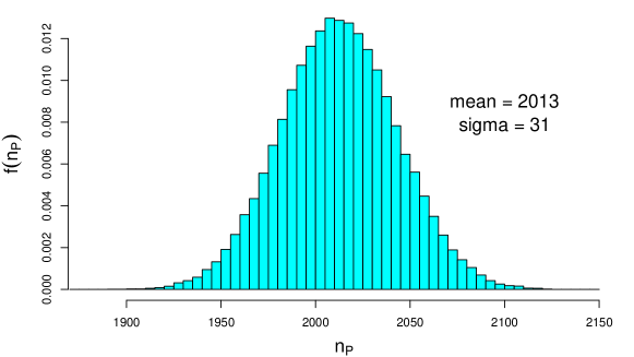
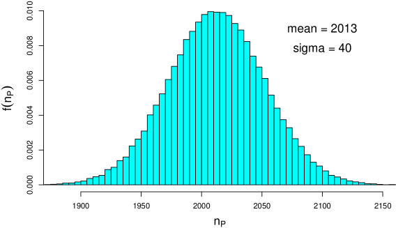
Figure 12: Probabilistic prediction of the numbers of positives in a sample of 10000 individuals taken from a population of 10000, 100000 and 1000000 individuals (in order, from top to bottom), 10% of which are infected ($p=0.1$), assuming $\pi_{1}=0.978$ and $\pi_{2}=0.115$.

Some results are shown in Fig. 12, where, for comparison with what we have seen in the previous sections, a sample size of 10000 individuals is used, taken from a population of 10000 (top histogram), 100000 (middle) and 1000000 (bottom), and assuming $p=0.1$. $[$Note that first case corresponds exactly to the assumed value of $p_{s}=0.1$ shown in the top plot of Fig. 10, since, being $n_{s}=N$, the standard uncertainty on $p_{s}$ vanishes.$]$ Increasing the population size the standard deviation increases, as an effect of $\sigma(p_{s})$, although this growth saturates for $N$ a bit higher than $\approx 10\times n_{s}$, above which the size dependent factor of Eq. (68) becomes negligible. In fact, the asymptotic value, given by Eq. (69) is in this case $\left.\sigma(p_{s})\right|_{N\rightarrow\infty}=0.0030$. For $N/n_{s}=10$ the standard uncertainty on $p_{s}$ becomes 0.00285, vanishing for $n_{s}=N$ (the value of 0.0015, half of the asymptotic one, is reached for $N=4/3\times n_{s}$).

6.2.1 Approximated results

It is interesting to compare the Monte Carlo results of Fig. 12 to those obtained by the approximated values of expected value and standard deviation given by Eqs. (59)-(60) just putting $\sigma(\pi_{1})=\sigma(\pi_{2})=0$. The contribution to the uncertainty due to the two binomials of Fig. 9 is $\sigma_{R}(n_{P})=30.6$ (rounded to 31 in Fig. 12), while those due to $\sigma(p_{s})$ are equal to 0, 24.6 and 25.9, for the three population sizes. The combined standard uncertainties are then 30.6, 39.3 and 40.1, in perfect agreement with the results shown in Fig. 12.

6.3 Detailed study of the four contributions to $\sigma(f_{P})$

At this point it is time to release the limiting assumption of exact values of sensitivity and specificity, i.e. $\sigma(\pi_{1})=\sigma(\pi_{2})=0$. Moreover, having checked that the approximated formulae can take into account with great accuracy also the contribution due to the uncertain value of $p_{s}$, we find it interesting and useful to study the individual contributions to the uncertainty with which we can forecast the fraction $f_{P}$ of tested individuals resulting positive. For the reader’s convenience, we summarize here the relevant, approximated expressions, making also use, in order to simplify them, of the equality $\mbox{E}(p_{s})=p$ :

$$\mbox{E}(f_{P}) \approx \mbox{E}(\pi_{1})\cdot p+\mbox{E}(\pi_{2})\cdot(1-p)$$ (71)

$$\sigma(f_{P}) \approx \sigma_{R}(f_{P})\oplus\sigma_{p_{s}}(f_{P})\oplus\sigma_{\pi_{1}}(f_{P})\oplus\sigma_{\pi_{2}}(f_{P})$$ (72)

$$\sigma_{R}(f_{P}) = \sqrt{\mbox{E}(\pi_{1})\cdot(1-\mbox{E}(\pi_{1}))\cdot p+\mbox{E}(\pi_{2})\cdot(1-\mbox{E}(\pi_{2}))\cdot(1-p)}/\sqrt{n_{s}}\ \$$ (73)

$$\sigma_{\pi_{1}}(f_{P}) = \sigma(\pi_{1})\cdot p$$ (74)

$$\sigma_{\pi_{2}}(f_{P}) = \sigma(\pi_{2})\cdot(1-p)\,.$$ (75)

$$\sigma_{p_{s}}(f_{P}) = \sigma(p_{s})\cdot|\mbox{E}(\pi_{1})-\mbox{E}(\pi_{2})|$$ (76)

$$\approx |\mbox{E}(\pi_{1})-\mbox{E}(\pi_{2})|\cdot\sqrt{p\cdot(1-p)\cdot(1-n_{s}/N)}/\sqrt{n_{s}}$$

We can note that $\sigma_{\pi_{2}}(f_{P})$ and $\sigma_{\pi_{1}}(f_{P})$ are independent of the sample size $n_{s}$, while $\sigma_{R}(f_{P})$ and $\sigma_{p_{s}}(f_{P})$ exhibit the typical ‘statistical dependence’ $\propto 1/\sqrt{n_{s}}$. Therefore we shall refer hereafter to $\sigma_{R}(f_{P})$ and $\sigma_{p_{s}}(f_{P})$ as random (or statistical) contributions; to the others as contributions due to systematics, which cannot be improved increasing the sample size.

The upper plot of Fig. 13

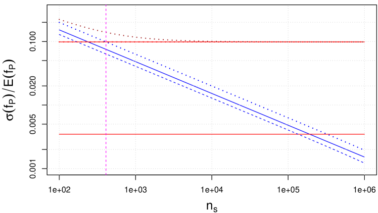
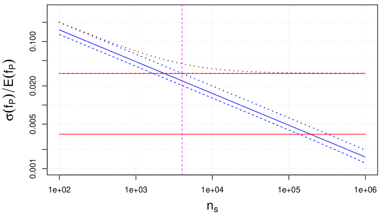
Figure 13: Contributions to the relative uncertainty on the fraction of positives as a function of the sample size $n_{s}$, assuming it much smaller than the population size $N$, for a proportion of infected individuals $p=0.1$. The solid blue line with negative slope is the contribution from $\sigma_{R}(f_{P})$, the dashed blue one is the contribution from $\sigma_{p_{s}}(f_{P})$, the dotted line is the ‘quadratic sum’ of the two; the lower horizontal red one is the contribution from $\sigma_{\pi_{1}}(f_{P})$ and the upper horizontal one is the contribution from $\sigma_{\pi_{2}}(f_{P})$ (a dotted red line, showing their ‘quadratic sum’ is indeed overlapping the $\pi_{2}$ contribution). The overall uncertainty is shown by the uppest curve (dotted brown). The upper plot is for a standard uncertainty on $\pi_{2}$ $\sigma(\pi_{2})=0.022$. The lower plot is for the case of uncertainty reduced to $\sigma(\pi_{2})=\sigma(\pi_{1})=0.007$.

shows, for our reference value of $p=0.1$ and for uncertain $\pi_{1}$ and $\pi_{2}$ (summarized as $\pi_{1}=0.978\pm 0.007$ and $\pi_{2}=0.115\pm 0.022$), the relative uncertainty on $f_{P}$, that is $\sigma(f_{P})/\mbox{E}(f_{P})$, as a function of $n_{s}$, highlighting the different contributions to the total uncertainty. The horizontal lines represent the two systematic contributions, independent from $n_{s}$, while their quadratic sum does not appears in the plot, because it overlaps practically exactly with the dominant systematic contribution, due to the uncertain $\pi_{2}$. The ‘straight lines with negative slopes’ (in log-log plot, which notoriously linearizes power laws) are the individual statistical contributions (solid and dashed, respectively – see the figure caption for details) and their quadratic sum (dotted). The uppest (dotted brown) curve is the overall uncertainty, dominated at small $n_{s}$ by the statistical contributions and at high $n_{s}$ by the systematic ones, namely by $\sigma_{\pi_{2}}(f_{P})$. (We shall come in a while into the meaning and the importance of the vertical line.)

Since the dominant contribution due to $\sigma(\pi_{2})$ limits the relative uncertainty on $f_{P}$ to about $10\%$, reached for $n_{s}$ above a few thousands, it is interesting to see what we would gain reducing $\sigma(\pi_{2})$ to the value of $\sigma(\pi_{1})$. This is done in the bottom plot of Fig. 13, which shows a clear improvement, although the contribution due to $\sigma(\pi_{2})$ still dominates with respect to that due to $\sigma(\pi_{1})$, because the former enters, for $p=0.1$, with a weight 9 times higher than the latter, as it results from Eqs. (74) and (75). Moreover, since all contributions to the uncertainty on $f_{P}$ depend also on $p$, we report in Fig. 14 the case of a supposed proportion of infectees as high as $50\%$ (i.e. $p=0.5$).

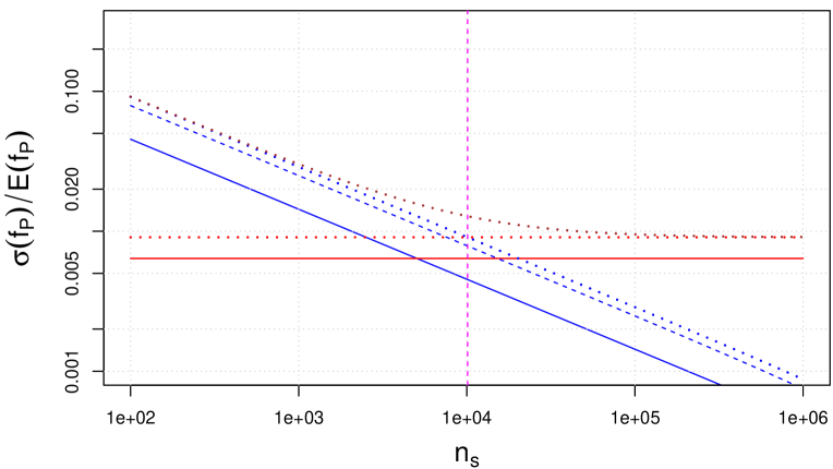
Figure 14: Same as Fig. 13 for a proportion of infected individuals of $50\%$ ($p=0.5$). In this case the contribution from sampling the population $\sigma_{p_{s}}(f_{P})$ is larger than that from $\sigma_{R}(f_{P})$. Note that in the lower plot the two solid horizontal lines collapse into a single one, being the contribution from $\sigma_{\pi_{1}}(f_{P})$ and $\sigma_{\pi_{2}}(f_{P})$ equal. It is, instead, visible, with respect to the plots of Fig. 13 the horizontal dotted line showing the quadratic combination of the systematic contributions, reached asymptotically by the top dotted curve representing the global relative uncertainty on $f_{P}$.

One of the remarkable difference with respect to Fig. 13 is that the contribution from $\sigma_{p_{s}}(f_{P})$ becomes larger than that from $\sigma_{R}(f_{P})$ (remaining always ‘parallel’ as a function of $n_{s}$ in ‘log-log’ plots, since they depend on the same power of the sample size). Indeed, $\sigma_{p_{s}}(f_{P})$ starts dominating from $p\approx 0.15$ up to $p\approx 0.95$, as shown in Fig. 15,

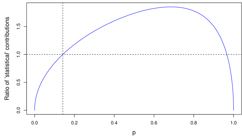
Figure 15: Ratio of $\sigma_{p_{s}}(f_{P})$ to $\sigma_{R}(f_{P})$ as a function of the population fraction of infected $p$.

in which the ratio $\sigma_{p_{s}}(f_{P})/\sigma_{R}(f_{P})$ as a function of $p$, is reported, exhibiting a whale-like shape.

As a further example we show in Fig. 16 the contributions

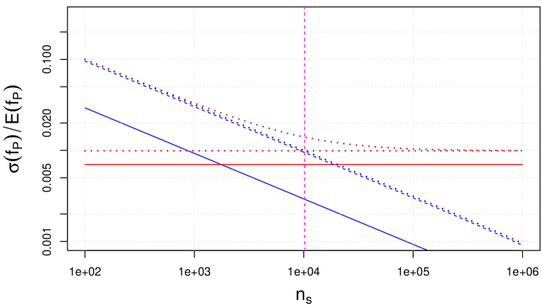
Figure 16: Same quantities of Figs. 13 and 14, but in the symmetric case of specificity equal to sensitivity, i.e. $\mbox{E}(\pi_{2})=1-\mbox{E}(\pi_{1})=0.022$, again with equal uncertainties, i.e. $\sigma(\pi_{2})=\sigma(\pi_{1})=0.007$. The upper plot, for $p=0.1$, has to be compared to the lower plot of Fig. 13; the lower plot, for $p=0.5$, has to be compared to the lower plot of Fig. 14.

to the relative uncertainty of $f_{P}$ for the case of improved specificity of the test, i.e. reducing the expected value of $\pi_{2}$ from 0.115 to 0.022, keeping its uncertainty equal to that of $\pi_{1}$, that is 0.007. This means that we consider specificity equal to sensitivity, both in expected value and in uncertainty. In practice this is done swapping the parameters of the related Beta distributions, that is $r_{2}=s_{1}$ and $s_{2}=r_{1}$ (see Sec. 4.2).

In order to make evident the differences with what has been shown in the previous cases, we plot $\sigma_{p_{s}}(f_{P})/\mbox{E}(f_{P})$ for both $p=0.1$ (upper plot) and $p=0.5$ (lower plot). In particular, in order to see the effect of this last improvement of the specificity (i.e. increasing its expected value from 0.885 to 0.978, keeping the same standard uncertainty) we need to compare the upper plot of Fig. 16 with the lower plot of Fig. 13; the lower plot of Fig. 16 with the lower plot of Fig. 14. The result is, at least at a first sight, quite counter-intuitive, since to a sizable improvement in specificity there is a reduction in the relative accuracy with which the fraction of positives is expected (effect particularly important for $p=0.1$). We shall comment about it in the next sub-section, in which we start describing the vertical lines in the plots of Figs. 13, 14 and 16, commenting on their importance.

6.4 Balance between statistical and systematic contributions to the uncertainty on $f_{P}$

The vertical dashed line in the plots of Figs. 13, 14 and 16 indicates the critical value $n_{s}^{*}$ at which the contribution to total uncertainty due to $\sigma_{\pi_{2}}(f_{P})$ and $\sigma_{\pi_{1}}(f_{P})$ is equal to that due to $\sigma_{R}(f_{P})$ and $\sigma_{p_{s}}(f_{P})$, that is for $n_{s}=n_{s}^{*}$ statistical and systematic contributions are equal. It follows that, due to the quadratic combination rule, the global uncertainty at that critical value of the sample size will be larger than each of them by a factor $\sqrt{2}$.

Being $n_{s}^{*}$ an important parameter in order to plan a test campaign, it is worth getting its closed, although approximated expression, obtained extending the condition (5.3) to

$$\sigma_{R}^{2}(f_{P})+\sigma_{p_{s}}^{2}(f_{P}) = \sigma_{\pi_{1}}^{2}(f_{P})+\sigma_{\pi_{2}}^{2}(f_{P})\,,$$ (77)

The result, under the minimal assumption $N\gg 1$, is

$$\begin{split}n_{s}^{*}=\frac{\big{[}\big{(}\mbox{E}(\pi_{1})-\mbox{E}(\pi_{2})\big{)}^{2}\!\cdot\!p\!\cdot\!(1-p)\big{]}+\big{[}\mbox{E}(\pi_{1})\!\cdot\!(1-\mbox{E}(\pi_{1}))\!\cdot\!p+\mbox{E}(\pi_{2})\!\cdot\!(1-\mbox{E}(\pi_{2}))\!\cdot\!(1-p)\big{]}}{\big{[}\sigma^{2}(\pi_{1})\cdot p^{2}+\sigma^{2}(\pi_{2})\cdot(1-p)^{2}\big{]}+\big{[}\left(\mbox{E}(\pi_{1})-\mbox{E}(\pi_{2})\right)^{2}\cdot p\cdot(1-p)\big{]}/N}\,.\end{split}$$ (78)

(Note how in the limit $N\gg n_{s}$, i.e. $N\rightarrow\infty$, the second term at the denominator of Eq. (78) can be neglected.) The top plot of Fig 17 shows the dependence of $n_{s}^{*}$ on $p$,

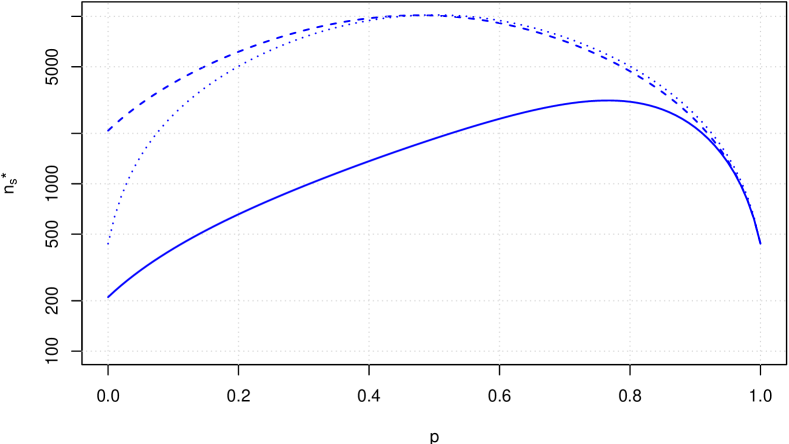
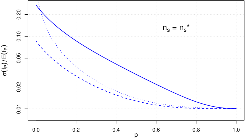
Figure 17: Top plot: dependence of $n_{s}^{*}$ on $p$ for the standard values of $\sigma_{\pi_{1}}$ and $\sigma_{\pi_{2}}$ (solid line), for $\sigma_{\pi_{1}}=\sigma_{\pi_{2}}=0.007$ (dashed line) and for specificity equal to sensitivity, i.e. $\mbox{E}(\pi_{2})=1-\mbox{E}(\pi_{1})=0.022$ (dotted line). Bottom plot: relative uncertainty on $f_{P}$ at $n_{s}=n_{s}^{*}$ for the same cases.

for: our reference values of $\sigma(\pi_{1})$ and $\sigma(\pi_{2})$ (solid line – see also top plots of Figs. 13 and 14); the improved case of $\sigma(\pi_{2})=\sigma(\pi_{1})=0.007$ (dashed line – see also bottom plots of Figs. 13 and 14); the mirror-symmetric case in which $\mbox{E}(\pi_{2})=1-\mbox{E}(\pi_{1})=0.022$ and $\sigma(\pi_{2})=\sigma(\pi_{1})=0.007$ (dotted line – see also Fig. 16). Once we know the dependence of $n_{s}^{*}$ on $p$, since the uncertainty on $f_{P}$ depends on $n_{s}$ and $p$, we can evaluate the relative uncertainty on the predicted fraction of positives that will result from the test campaign, as a function of $p$ under the condition $n_{s}=n_{s}^{*}$, that is $\left.\sigma(f_{P})/\mbox{E}(f_{P})\right|_{n_{s}=n_{s}^{*}}$. The result is shown in the bottom plot of Fig 17 for the three cases of the upper plot of the same figure.

When we reduce the uncertainty about $\sigma(\pi_{2})$, keeping constant its expected value, the systematic contribution to the uncertainty is reduced and then, as we have already learned from Figs. 13, 14 and 16, it becomes meaningful to analyze larger samples. We can then predict the fraction of individuals tagged as positive with improved accuracy, i.e. $\sigma(f_{P})/\mbox{E}(f_{P})$ decreases. This intuitive reasoning is confirmed by the plots of Fig 17, moving from the solid curves to the dashed ones. Instead, improving the specificity to 0.885 to 0.978, i.e. reducing $\mbox{E}(\pi_{2})$ from 0.115 to 0.022, keeping the same uncertainty of 0.007, leads to surprising results at low values of $p$, at least at a first sight (dashed curves $\rightarrow$ dotted curves). In fact, one would expect that from this further improvement in the quality of the test (which definitively makes a difference when testing a single individual, as discussed in Sec. 4) should follow a general improvement in the prediction of the fraction of positives.

The reason of this counter-intuitive outcome is due to the combination of two effects. The first is the dependence on $\mbox{E}(\pi_{1})$ and $\mbox{E}(\pi_{2})$ of the statistical contributions to the uncertainty, as we can see from Eqs. (73) and (76). The second is that, decreasing $\mbox{E}(\pi_{2})$, the expected value of $f_{P}$ decreases too (less ‘false positives’) and therefore the relative uncertainty on $f_{P}$, i.e. $\sigma(f_{P})/\mbox{E}(f_{P})$, increases. While the second effect is rather obvious and there is little to comment, we show the first one graphically, for $p=0.1$ at which the effects becomes sizable, in the three plots of Fig. 18:

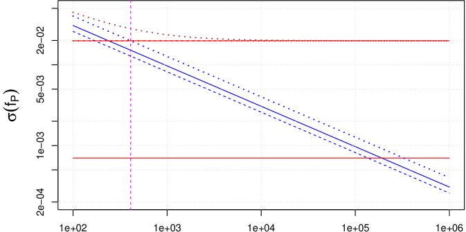
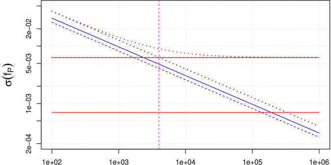
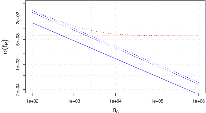
Figure 18: Contributions to $\sigma(f_{P})$ varying $\sigma(\pi_{2})$ and $\mbox{E}(\pi_{2})$ for $p=0.1$ (see text).

the upper plot for our reference values of $\pi_{1}$ and $\pi_{2}$, the middle one improving $\sigma(\pi_{2})$ to 0.007, and the bottom one also reducing the expected value of $\pi_{2}$ to 0.022. But differently from Figs. 13, 14 and 16, these plots show $\sigma(f_{P})$ instead of $\sigma(f_{P})/\mbox{E}(f_{P})$, so that we can focus only on the contributions to the uncertainty, not ‘distracted’ by the variation of the expected value of $f_{P}$. Moving from the top plot to the middle one, only the contribution due to $\pi_{2}$ is reduced, all the others remaining exactly the same. Then, when we increase the specificity, i.e. we reduce $\mbox{E}(\pi_{2})$ from 0.115 to 0.022, keeping unaltered its uncertainty, its contribution to $\sigma(f_{P})$ is unaffected, while the statistical contributions do change. In particular $\sigma_{R}(f_{P})$ is strongly reduced, while $\sigma_{p_{s}}(f_{P})$ increases a little bit. The combined effect is a decrease of the overall statistical contribution, thus lowering $n_{s}^{*}$.

Summing up, the combination of the two plots of Fig. 17 gives at a glance, for an assumed proportion of infectees $p$, an idea of the ‘optimal’ relative uncertainty we can get on $f_{P}$ (bottom plot) and the sample size needed to achieve it (upper plot). We remind that the lowest relative uncertainty, equal to $1/\sqrt{2}$ of the value shown in the plot, is reached when the sample size $n_{s}$ is about one order of magnitude larger than $n_{s}^{*}$, i.e. when the random contribution to the uncertainty is absolutely negligible and any further increase of $n_{s}$ not justifiable. But, anyway – think about it – being $1/\sqrt{2}\approx 0.7$, is it worth increasing so much ($\approx 10$ times) the sample size in order to reduce $\sigma(f_{P})$ by only 30%?

         

Figure 19: Graphical network of Fig. 9, augmented by the sampling process, modeled by a hypergeometric distribution (left) or by a binomial distribution (right) with $p=N_{I}/(N_{I}+N_{NI})$.

7 Measurability of $p$

It is now time to put together all the items discussed so far and to move to the question of how well we can measure the proportion $p$ of infectees in a population of $N$ individuals, out of which $n_{s}$ have been sampled at random and tested, resulting in a total of $n_{P}$ positives. Again we proceed by steps. In this section we tackle the question of how the expected number of positives and its uncertainty depend on the proportion $p$ of infectees in the population. The real inferential problem, consisting in stating which values of $p$ are more or less believable, will be analyzed in Secs. 8 and 9.

7.1 Probabilistic model

The graphical model describing the quantities of interest is shown in the left hand network of Fig. 19, based on that of Fig. 9, to which we have added parents to the nodes $n_{I}$ and $n_{NI}$, the number of Infected and Not Infected in the sample, respectively. More precisely, the number of infectees $n_{I}$ in the sample is described by a hypergeometric distribution, that is

$$n_{I} \sim \mbox{HG}(N_{I},N_{NI},n_{s})\,,$$

with $N_{I}$ and $N_{NI}$ the numbers of infected and not infected individuals in the population. Then, the number $n_{NI}$ of not infected people in the sample is deterministically related to $n_{I}$, being $n_{NI}=n_{s}-n_{I}$.

However, since in this paper we are interested in sample sizes much smaller than those of the populations, we can remodel the problem according to the right hand network of Fig. 19, in which $n_{I}$ is described by a binomial distribution, that is

$$n_{I} \sim \mbox{Binom}(n_{s},p)\,,$$

with $p=N_{I}/(N_{I}+N_{NI})$. This simplified model has been re-drawn in the network shown in the left hand side of Fig. 20,

   

Figure 20: Simplified graphical model of Fig. 19 rewritten in order to make explicit ‘known’/‘assumed’ quantities, tagged by the symbol ’$\surd\,$’, and the uncertain ones. In particular, in the left hand diagram precise values of $\pi_{1}$ and $\pi_{2}$ are assumed, while in the the right hand one the uncertainty on their values is modeled with Beta pdf’s with parameters $(r_{1},s_{1})$ and $(r_{2},s_{2})$.

indicating by the symbol ‘$\surd\,$’ the certain variables in the game (indeed those which are for some reason assumed), in contrast to the others, which are uncertain and whose values will be ranked in degree of belief following the rules of probability theory. Note that in this diagram $\pi_{1}$ and $\pi_{2}$ are assumed to be exactly known. Instead, as we have already seen in Sec. 4, their values are uncertain and their probability distribution can be conveniently modeled by Beta probability functions characterized by parameters $r$’s and $s$’s. The graphical model which takes into account also the uncertainty about $\pi_{1}$ and $\pi_{2}$ is drawn in the same Fig. 20 (right side).

We have already discussed extensively, in Sec. 6, how the expectation of $n_{P}$, and therefore of the fraction on positives in the sample, $f_{P}$, depends on the model parameters. Now we go a bit deeper into the question of the dependence of $f_{P}$ on the fraction of infectees in the population and, more precisely, which are the ‘closest’ (to be defined somehow) two values of $p$, such that the resulting $f_{P}$’s are ‘reasonably separated’ (again to be defined somehow) from each other. Moreover, instead of simply relying on the approximated formulae developed in Sec. 6, we are going to use Monte Carlo methods in different ways: initially just based on R random number generators; then using (well below its potentials!) the program JAGS, which will then be used in Sec. 8 for inferences. However we shall keep using the approximated formulae for cross check and to derive some useful, although approximated, results in closed form.

7.2 Monte Carlo estimates of $f(n_{P})$ and $f(f_{P})$

Analyzing the graphical model in the right hand side of Fig. 20, the steps we have to go through become self-evident:

1. generate a value of $n_{I}$ according to a binomial distribution, then calculate $n_{NI}$;

2. generate a value of $\pi_{1}$ and of $\pi_{2}$ according to Beta distributions;

3. generate a value of $n_{P_{I}}$ and a value of $n_{P_{NI}}$ according to binomial distributions;

4. sum up $n_{P_{I}}$ and $n_{P_{NI}}$ in order to get $n_{P}$.

7.2.1 Using the R random number generators

The implementation in R is rather simple, thanks also to the capability of the language to handle ‘vectors’, meant as one dimensional arrays, in a compact way. The steps described above can then be implemented into the following lines of code:

n.I   <- rbinom(nr, ns, p)       # 1.
n.NI  <- ns - n.I
pi1   <- rbeta(nr, r1, s1)       # 2.
pi2   <- rbeta(nr, r2, s2)
nP.I  <- rbinom(nr, n.I, pi1)    # 3.
nP.NI <- rbinom(nr, n.NI, pi2)
nP    <- nP.I + nP.NI            # 4.

We just need to define the parameters of interest, including nr, number of extractions, run the code and add other instructions in order to print and plot the results (a minimalist script performing all tasks is provided in Appendix B.5). The only instructions worth some further comment are the two related to the step nr. 3. A curious feature of the ‘statistical functions’ of R is that they can accept vectors for the number of trials and for probability at each trial, as it is done here. It means that internally the random generator is called nr times, the first time e.g. with n.I$[$1$]$ and pi1$[$1$]$, the second time with n.I$[$2$]$ and pi1$[$2$]$, and so on, thus avoiding us to use explicit loops. Note that, if precise values of $\pi_{1}$ and $\pi_{2}$ were assumed, then we just need to replace the two lines of step nr. 2 with the assignment of their numeric values.

Figure 21 shows the results

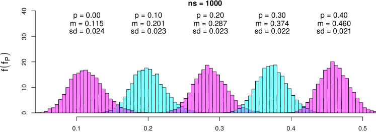
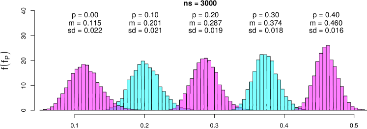
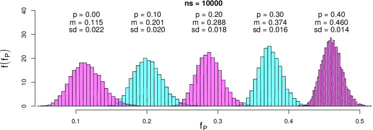
Figure 21: Predictive distributions of $f_{P}$ as a function of $p$ and $n_{s}$ for our default uncertainty on $\pi_{2}$, summarized as $\pi_{2}=0.115\pm 0.022$.

obtained for some values of $p$ and $n_{s}$, and modeling the uncertainty of $\pi_{1}$ and $\pi_{2}$ in our default way, summarized by $\pi_{1}=0.978\pm 0.007$ and $\pi_{2}=0.115\pm 0.022$. The values of $n_{s}$ have been chosen in steps of roughly half order of magnitude in the region of $n_{s}^{*}$ of interest, as we have learned in Sec. 6. We see that for the smallest $n_{s}$ shown in the figure, equal to 300, varying $p$ by 0.1 produces distributions of $f_{P}$ with quite some overlap. Therefore with samples of such a small size we can say, very qualitatively that we can resolve different values of $p$ if they do not differ less than $\approx{\cal O}(0.1)$. The situations improves (the separation roughly doubles) when we increase $n_{s}$ to 1000 or even to 3000, while there is no further gain reaching $n_{s}=10000$. This is in agreement with what we have learned in the previous section.

Since, as we have already seen, the limiting effect is due to systematics, and in particular, in our case, to the uncertainty about $\pi_{2}$, we show in Fig. 22

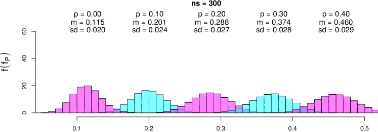
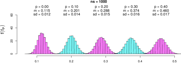
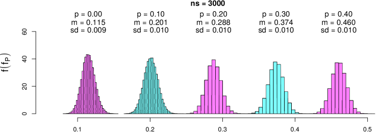
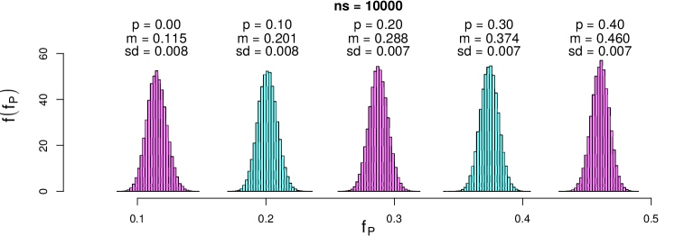
Figure 22: Same as Fig. 21, but for an improved knowledge of $\pi_{2}$, summarized as $\pi_{2}=0.115\pm 0.007$.

how the result changes if we reduce $\sigma(\pi_{2})$ to the level of $\sigma(\pi_{1})$. As we can see (a result largely expected), there is quite a sizable improvement in separability of values of $p$ for large values of $n_{s}$. Again qualitatively, we can see that values of $p$ which differ by $\approx{\cal O}(0.01)$ can be resolved.

Finally we show in Fig. 23

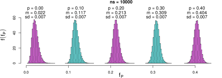
Figure 23: Same as Fig. 22, but for an improved specificity, summarized as $\pi_{2}=0.022\pm 0.007$.

the case in which sensitivity and specificity are equal, both as expected value and standard uncertainty. The first thing we note in these new histograms is that for $p=0$ they are no longer symmetric and Gaussian-like. This is due to the fact that no negative values of $n_{P}$ are possible, and then there is a kind of ‘accumulation’ for low values of $n_{P}$, and therefore of $f_{P}$ (this kind of skewness is typical of all probability distributions of variables defined to be positive and whose standard deviation is not much smaller than the expected value – think e.g. at a Poissonian with $\lambda=2$).

7.2.2 Using JAGS

Let us repeat the Monte Carlo simulation improperly using the program JAGS [10], interfaced to R via the package rjags [12]. JAGS is a powerful tool developed, as open source, multi-platform clone of BUGS, to perform Bayesian inference by Markov Chain Monte Carlo (MCMC) using the Gibbs Sampler algorithm, as its name reminds, acronym of Just Another Gibbs Sampler. For the moment we just get familiar with JAGS using it as kind of ‘curious’ random generator.

The first thing to do is to write down the probabilistic model that relates the different variables that enter the game. For example, the left hand graphical model of Fig. 20 is implemented in JAGS by the following self-explaining piece of code

model {
  n.I ~ dbin(p, ns)
  n.NI <- ns - n.I
  nP.I ~ dbin(pi1, n.I)
  nP.NI ~ dbin(pi2, n.NI)
  nP ~ sum(nP.I, nP.NI)
  fP <- nP / ns
}

in which we have added the last instruction to model the trivial node (not shown in Fig. 20) relating in a deterministic way fP to nP and ns. In the model the symbol ‘$\sim$’ indicates that, e.g. n.I is described by a binomial distribution defined by p and ns (be aware of the different order of the parameters with respect to the R function!), while ‘$<\!\!\!-$’ stands for a deterministic relation (indeed the symbols of assignment in R). A nice thing of such a model is that the order of the instructions is not relevant. In fact it is only needed – let us put it so – to describe the related graphical model. All the rest will be done internally by JAGS at the compilation step.

Then, obviously, we have to

• pass to the program the model parameters (observed nodes), which are p, ns, pi1 and pi2;

• instruct it on how many ‘iterations’ to do;

• analyze, among all unobserved nodes (n.I, n.NI, nP.I, nP.NI, nP and fP), the ones of interest, the most important one being, for us, fP.

Moving to the second model of Fig. 20, in which we also take into account the uncertainty about $\pi_{1}$ and $\pi_{2}$, is straightforward: we just need to add two instructions to tell JAGS that pi1 and pi2 are indeed unobserved and that they depend on r1, s1, r2 and s2:

model {
  n.I ~ dbin(p, ns)
  n.NI <- ns - n.I
  nP.I ~ dbin(pi1, n.I)
  nP.NI ~ dbin(pi2, n.NI)
  pi1 ~ dbeta(r1, s1)
  pi2 ~ dbeta(r2, s2)
  nP ~ sum(nP.I, nP.NI)
  fP <- nP / ns
}

Once the model is defined, it has to be saved into a file, whose location is then passed to JAGS (we shall regularly use the temporary file tmp_model.bug, whose extension ‘.bug’ is the BUGS/JAGS default).

At this point, moving to the R code to interact with JAGS, we need to

• load the interfacing package rjags;

• prepare a R ‘list’ containing the data (in particular, the values of the ‘observed’ nodes);

• call jags.model() to ‘setup’ the model;

• call coda.samples() to ask JAGS to perform the sampling, also specifying the variables we want to monitor, whose ‘histories’ will be returned in a single ‘object’.

Finally we have to show the result. All this is done, for example, in the R script provided in Appendix B.6 (note that the temporary model file is written directly from R, a convenient solution for small models). Needless to say, we get, apart from statistical fluctuations inherent to Monte Carlo methods, ‘exactly’ the same results obtained with the script of Appendix B.5, which only uses R statistical functions.

7.2.3 Further check of the approximated formulae

Finally, we have checked the validity of the approximated formulae (71)-(76) to evaluate the expected value and the standard uncertainty of $f_{P}$ in all cases considered in Figs.  21-23. The agreement is indeed excellent, even in the cases of $p=0$ of Fig. 23, characterized by skewed distributions. The R script to reproduce all numbers of all three figures is provided in Appendix B.7.

7.3 Resolution power

Having to turn the qualitative judgment regarding the ‘separation’ of the distributions of $f_{P}$ for different $p$, as it results from Figs. 21-23, into a resolution power, one needs some convention. First, we remind that, unless $p$ is very small, we have good theoretical reasons, confirmed by Monte Carlo simulations, that $f_{p}$ is about Gaussian, at least in the range of a few standard deviations around its mean value. But Gaussian curves are, strictly speaking, never separated from each other, because they have as domain the entire real axis for all $\mu$’s and $\sigma$’s. In fact this is a “defect” of such distribution, as Gauss himself called it [30] and some grain of salt is required using it. In order to form an idea of how one could define conventionally ‘resolution’, the upper plot of Fig. 24 shows

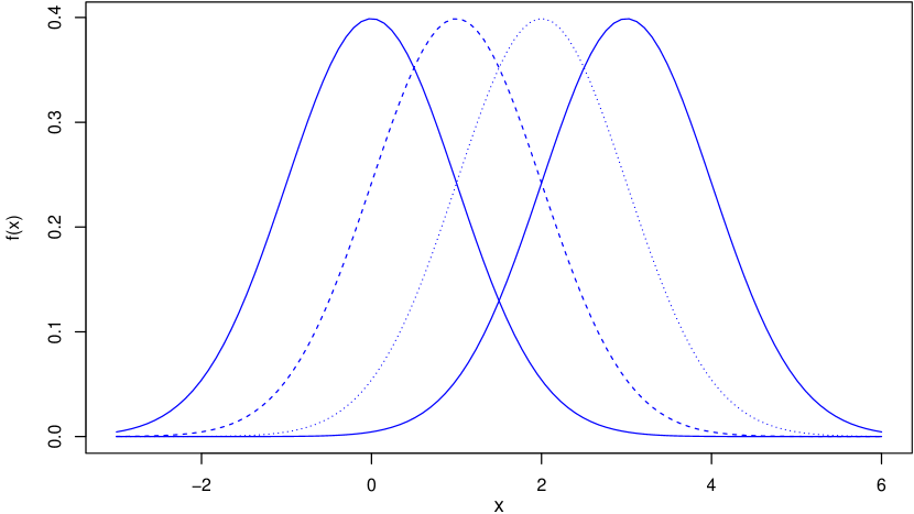
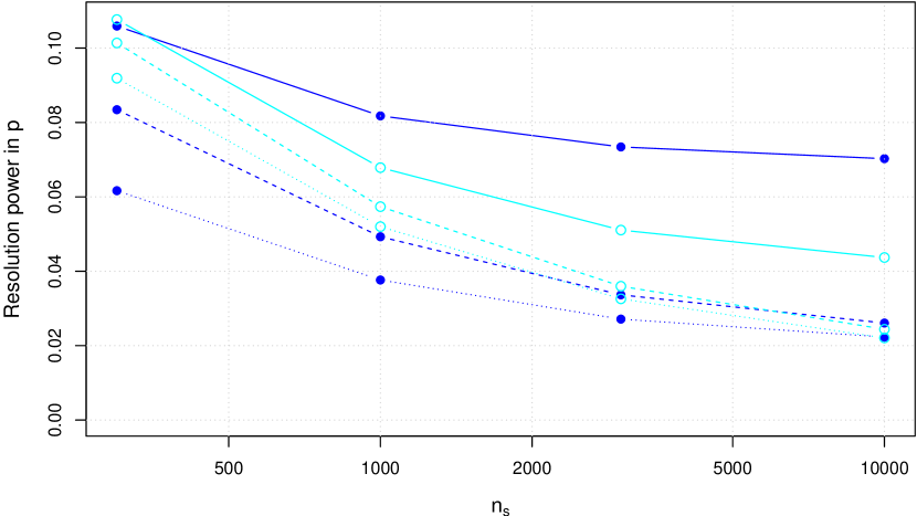
Figure 24: Upper plot: Examples of Gaussians whose $\mu$ parameters are separated by 1 $\sigma$. Bottom plot: resolution power in $p$, defined by Eq. (80), for $\kappa=3$ (lines between points just to guide the eye). Filled (blue) circles for $p=0.1$ and open (cyan) circles for $p=0.5$. Solid lines for $\pi_{2}=0.115\pm 0.022$, dashed lines for $\pi_{2}=0.115\pm 0.007$ and dotted lines for $\pi_{2}=0.022\pm 0.007$ ($\pi_{1}=0.978\pm 0.007$ in all cases).

some Gaussians having unitary $\sigma$, with $\mu$’s differing by one $1\sigma$.

We see that a ‘reasonable separation’ is achieved when they differ by a few $\sigma$’s – let us say, generally speaking, $\kappa\,\sigma$, although absolute separation can never occur, for the already quoted intrinsic “defect” of the distribution. Having to choose a value, we just opt arbitrarily for $\kappa=3$, corresponding to the two solid lines of the figure, although the conclusions that follow from this choice can be easily rescaled at wish. Moreover, as we can see from Figs. 21-23 (and as it results from the approximated formulae)

• the standard deviation of the distributions varies smoothly with $p$;

• the mean value depends linearly on $p$ for obvious reasons.

Therefore the resolution power in the interval $[p,p+\Delta p]$ can be evaluated by a simple proportion

$${\cal R}(p,p+\Delta p) \approx \frac{\Delta p}{\left.\mbox{E}(f_{P})\right|_{p+\Delta p}-\left.\mbox{E}(f_{P})\right|_{p}}\cdot\kappa\cdot\left.\sigma(f_{P})\right|_{p+\Delta p/2}\,.$$ (79)

For example, using the numbers of the Monte Carlo evaluations shown in Fig. 21, for $p=0.1$ and $n_{s}=300$ we get $0.1/(0.288-0.201)\times 3\times 0.0305=0.105$, reaching at best $\approx 0.022$ in the case of $n_{s}=10000$ shown in Fig. 23. The resolution power at a given value of $p$, is obtained in the limit ‘$\Delta p\rightarrow 0$’:

$${\cal R}(p) \approx \frac{\Delta p}{\left.\mbox{E}(f_{P})\right|_{p+\Delta p}-\left.\mbox{E}(f_{P})\right|_{p}}\cdot\kappa\cdot\left.\sigma(f_{P})\right|_{p}\,\hskip 22.76228pt(\Delta p\rightarrow 0).$$ (80)

The bottom plot of Fig. 24 shows the variation of the resolution power in $p$ for the same values of $n_{s}$ of Figs. 21-23 and for the usual cases of $\pi_{1}$ and $\pi_{2}$ of those figures (in the order: solid, dashed and dotted line – the lines are drawn just to guide the eye and to easily identify the conditions). The resolution power has been evaluated using the approximated formulae, for $\kappa=3$, around $p=0.1$ (blue filled circles) and around $p=0.5$ (cyan open circles), using for the gradient $\Delta p=0.01$ (the exact value is irrelevant for the numerical evaluation, provided it is small enough). $[$Obviously, if one prefers a different value of $\kappa$ (in particular one might like $\kappa=1$), then one just needs to rescale the results.$]$

7.4 Predicting the fractions of positives obtained sampling two different populations

An interesting question then arises: what happens if we measure, using tests having the same uncertainties on sensitivity and specificity, two different populations, having proportions of infectees $p^{(1)}$ and $p^{(2)}$, respectively? For example, in order to make use of results we have got above, let us take the results shown in Fig. 21 for $n_{s}=10000$, $p^{(1)}=0.1$ and $p^{(2)}=0.2$. For this value of the sample size and for our standard hypotheses for sensitivity and specificity, summarized as $\pi_{1}=0.978\pm 0.007$ and $\pi_{2}=0.115\pm 0.022$, the uncertainties are dominated by the systematic contributions. Our expectations are then $f_{P}^{(1)}=0.201\pm 0.020$ and $f_{P}^{(2)}=0.288\pm 0.018$. The difference of expectations is therefore $\Delta f_{P}=f_{P}^{(2)}-f_{P}^{(1)}=0.087$.

Now it is interesting to know how much uncertain this number is. One could improperly use a quadratic combination of the two standard uncertainties, thus getting $\Delta f_{P}=0.087\pm 0.027$. But this evaluation of the uncertainty on the difference is incorrect because $f_{P}^{(1)}$ and $f_{P}^{(2)}$ are obtained from the same knowledge of $\pi_{1}$ and $\pi_{2}$, and are therefore correlated. Indeed, in the limit of negligible uncertainties on these two parameters, the expectations would be much more precise, as we can see from the upper plot of Fig. 13, with a consequent reduction of $\sigma(\Delta f_{P})$. These are the results, obtained by Monte Carlo evaluation using only R commands (see script in Appendix B.8), with one extra digit with respect to Fig. 21 and adding also the correlation coefficient:

$$f_{P}^{(1)} = 0.2013\pm 0.0199$$

$$f_{P}^{(2)} = 0.2876\pm 0.0179$$

$$\Delta f_{P} = 0.0863\pm 0.0064$$

$$\rho\left(f_{P}^{(1)},f_{P}^{(2)}\right) = 0.9470$$

The uncertainty on $\Delta f_{P}$ is about one fourth of what naively evaluated above and about one third of the individual predictions, due to the well known effect of (at least partial) cancellations of uncertainties in differences, due to common systematic contributions. In this case, in fact, the standard deviation of $\Delta f_{P}$, calculated from standard deviations and correlation coefficient, is given by

$$\sigma(\Delta f_{P}) = \sqrt{\sigma^{2}(f_{P}^{(1)})+\sigma^{2}(f_{P}^{(2)})-2\,\rho\left(f_{P}^{(1)},f_{P}^{(2)}\right)\cdot\sigma(f_{P}^{(1)})\cdot\sigma(f_{P}^{(2)})}\,\,=\,\,0.0064\,,$$

in perfect agreement with what we get from Monte Carlo sampling.

An important consequence of the correlation among the predictions of the numbers of positives in different populations is that we have to expect a similar correlation in the inference of the proportion of infectees in different populations. This implies that we can measure their difference much better than how we can measure a single proportion. And, if one of the two proportions is precisely known using a different kind of test, we can take its value as kind of calibration point, which will allow a better determination also of the other proportion. We shall return to this interesting point in Sec. 8.6.

8 Inferring $p$ from the observed number of positives in the sample

Let us finally move to the probabilistic inference of the proportion of infected individuals, $p$, based on the number of positives $n_{P}$ in a sample of size $n_{s}$ and given our best knowledge of the performance of the test, all summarized in the graphical model of Fig. 25,

Figure 25: Graphical model of Fig. 20, re-drawn in order to emphasize its inferential use and including the commands to build up the JAGS model. ‘$f_{0}(p)$’, left open in this diagram, stands for the prior distribution of $p$.

which differs from that of Fig. 20 only for the symbol ‘$\surd$ ’ moved from node $p$ (now ‘unobserved’) to node $n_{P}$ (now ‘observed’). The diagram contains also the probabilistic and deterministic relations among the nodes, written directly using the JAGS language.

8.1 From the general problem to its implementation in JAGS

The most general problem would be to evaluate the joint conditional probability of the uncertain (‘unobserved’) quantities, conditioned by the ‘observed’ (‘known’/ ‘assumed’/‘postulated’) ones, that is, in this case (see Appendix A),

$$f(p,n_{I},n_{NI},n_{P_{I}},n_{P_{NI}},\pi_{1},\pi_{2}\,|\,n_{P},n_{s},r_{1},s_{1},r_{2},s_{2})\,,$$ (81)

although in practice we are indeed interested in $f(p\,|\,n_{P},n_{s},r_{1},s_{1},r_{2},s_{2})$, and perhaps in $f(n_{I}\,|\,n_{P},n_{s},r_{1},s_{1},r_{2},s_{2})$ and $f(n_{P_{I}}\,|\,n_{P},n_{s},r_{1},s_{1},r_{2},s_{2})$. This is done marginalizing Eq. (81) i.e. summing (or integrating, depending on their nature) over the variables on which we are not interested (see Appendix A). As commented in the same appendix, Eq. (81) is obtained, apart from a normalization factor, from

$$f(p,n_{I},n_{NI},n_{P_{I}},n_{P_{NI}},\pi_{1},\pi_{2},n_{P},n_{s},r_{1},s_{1},r_{2},s_{2}),$$ (82)

and the latter from a properly chosen chain rule. The steps used to build up Eq. (82) by the proper chain rule are exactly the instructions given to JAGS to set up the model, if we start from the bottom of the diagram of Fig. 25 and ascend through the parents (see Sec. 7.2.2):

model {
  nP ~ sum(nP.I, nP.NI)
  nP.I ~ dbin(pi1, n.I)
  nP.NI ~ dbin(pi2, n.NI)
  pi1 ~ dbeta(r1, s1)
  pi2 ~ dbeta(r2, s2)
  n.I ~ dbin(p, ns)
  n.NI <- ns - n.I
  p ~ dbeta(r0,s0)
}

The differences with respect to the JAGS model of Sec. 7.2.2 are

• the last instruction there, ‘fP $<$- nP/ns’, is here irrelevant;

• we have to add a prior to p, because all unobserved nodes having no parents need a prior (for practical convenience, as we have seen in Sec. 4.2, we shall use a Beta distribution, as indicated in the code);

• the sequence of the statements has been changed, but this has been done only in order to stress the analogy with the chain rule constructed ascending the graphical model of Fig. 25 (let us remind that the order is irrelevant for JAGS, which organizes all statements at the stage of compilation).

Hereafter we proceed using, very conveniently, JAGS, showing in Sec. 9 the steps needed from writing down the chain rule till the exact evaluation of $f(p)$ after marginalization.

8.2 Inferring $p$ and $n_{I}$ with our ‘standard parameters’

Let us start using as $n_{P}$ the expected value of positives of $\approx 2010$, obtained from what has been our starting set of parameters through the paper, that is $p=0.1$ with $n_{s}=10000$, with the uncertain parameters $\pi_{1}$ and $\pi_{2}$ modeled by Beta distributions with $(r_{1}=409.1,\,s_{1}=9.1)$ and $(r_{2}=25.2,\,s_{2}=193.1)$, respectively. Also for the prior of $p$ we use a Beta, starting with $r_{0}=s_{0}=1$, that models a flat prior, although we obviously do not believe that $p=0$ or $p=1$ are possible. We shall discuss in Sec. 8.7 the role of such at a first glance an insane prior (see also Sec. 9).

These are the R command to set the parameters of the game, call JAGS and show some results (for the complete script see Appendix B.10).

#---- data and parameters
nr = 1000000
ns = 10000
nP = 2010
r0 = s0 = 1
r1 = 409.1; s1 = 9.1
r2 = 25.2;  s2 = 193.1

# define the model and load rjags (omitted)
# .........................................

#---- call JAGS ---------
data <- list(ns=ns, nP=nP, r0=s0, s0=s0, r1=r1, s1=s1, r2=r2, s2=s2)
jm <- jags.model(model, data)
update(jm, 10000)
to.monitor <-  c(’p’, ’n.I’)
chain <- coda.samples(jm, to.monitor, n.iter=nr)

#---- show results
print(summary(chain))
plot(chain, col=’blue’)

Here are the results shown by ‘summary(chain)’

1. Empirical mean and standard deviation for each variable,
   plus standard error of the mean:

         Mean        SD  Naive SE Time-series SE
n.I 991.12477 225.85901 2.259e-01      16.079460
p     0.09919   0.02278 2.278e-05       0.001601

2. Quantiles for each variable:

         2.5%       25%      50%       75%     97.5%
n.I 506.00000 838.00000 1012.000 1153.0000 1389.0000
p     0.05046   0.08372    0.101    0.1155    0.1396

So, for this run we get $p=0.0992\pm 0.023$ and a number of infectees in the sample equal to $991\pm 226$, in agreement with our expectations. The results of the Monte Carlo sampling are shown in the ‘densities’ of Fig. 26,

Figure 26: Plots showing some JAGS results (see text).

together with the ‘traces’, i.e. the values of the sampled variables during the $10^{6}$ iterations. As it is easy to guess and as it appears from the two traces of the figure, there is some degree of correlation between the two variables, because they are obtained in a joint inference. The correlation is made evident in the scatter plot of Fig. 27

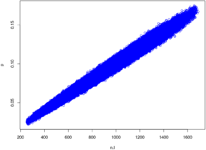
Figure 27: Scatter plot of $p$ vs $n_{I}$, showing the very high correlation between the two variables.

and quantified by $\rho(p,n_{I})=0.9914.\,$

Ωchain.df <- as.data.frame( as.mcmc(chain) )Ωplot(chain.df, col=’blue’)Ωcor(chain.df)Ω\end{verbatim}Ω

8.3 Dependence on our knowledge concerning $\pi_{1}$ and $\pi_{2}$

As we have already well understood, the uncertainty on the result is highly dependent of the uncertainty concerning $\pi_{1}$ and $\pi_{2}$. Therefore, as we have done in the previous sections, let us also change here our assumptions and see how the main result changes accordingly ($n_{I}$ is of little interest, at this point, also because of its very high correlation with $p$, and hence we shall not monitor it any longer in further examples).

1. First we start assuming negligible uncertainty on sensitivity and specificity.

   Ωa=1e6; r1=r1*a; s1=s1*a; r2=r2*a; s2=s2*aΩ\end{verbatim}Ω\mbox{} \vspace{-0.6cm} \mbox{}Ω
   

   As a result, the standard uncertainty $\sigma(p)$ becomes $0.0046$, that is about a factor $\approx 5$ smaller.

2. Then, as we have done in the above sections, we keep $\pi_{1}$ to its default value ($r_{1}=409.1,s_{1}=9.1$), only reducing the uncertainty of $\pi_{2}$ to $0.007$.

   Ωa=(22/7)^2; r2=r2*a; s2=s2*aΩ\end{verbatim}Ω\mbox{} \vspace{-0.6cm} \mbox{}Ω
   

   Also in this case the uncertainty decreases, getting $\sigma(p)=0.0085$.

3. Finally, we make the pdf of $\pi_{2}$ mirror symmetric with respect to that of $\pi_{1}$, that is $r_{2}=9.1,s_{2}=409.1$. But, obviously we need to change the number of the observed positives, choosing this time 1170, as suggested by our expectations (see Fig. 23). As a result we get $p=0.0995\pm 0.0076$, with an uncertainty not differing so much with respect to the previous case. Indeed, as we have have already noted in the previous sections, improving the specificity ($\pi_{2}$ reduced by a factor five) has only a little effect on the quality of the measurement, being more important the uncertainty with which that test parameter is known. (And we expect that something like that is also true for the sensitivity.)

8.4 Quality of the inference as a function of the sample size and of the fraction of positives in sample

A more systematic study of the quality of the inference is shown in Tab. 3,

$n_{s}$	$[n_{P}]$
	$\mbox{E}(p)\pm\sigma(p)$
300	[34]	[60]	[86]	[112]	[138]	[164]
	$0.026\pm 0.019$	$0.100\pm 0.034$	$0.200\pm 0.036$	$0.299\pm 0.037$	$0.399\pm 0.037$	$0.495\pm 0.036$
1000	[115]	[201]	[288]	[374]	[460]	[546]
	$0.021\pm 0.015$	$0.099\pm 0.028$	$0.198\pm 0.026$	$0.298\pm 0.025$	$0.399\pm 0.024$	$0.498\pm 0.023$
3000	[345]	[604]	[863]	[1122]	[1381]	[1640]
	$0.018\pm 0.014$	$0.099\pm 0.024$	$0.198\pm 0.023$	$0.299\pm 0.020$	$0.399\pm 0.019$	$0.499\pm 0.017$
10000	[1150]	[2013]	[2876]	[3739]	[4602]	[5465]
	$0.018\pm 0.013$	$0.099\pm 0.022$	$0.198\pm 0.020$	$0.299\pm 0.019$	$0.399\pm 0.016$	$0.499\pm 0.015$
300	[34]	[60]	[86]	[112]	[138]	[164]
	$0.019\pm 0.015$	$0.101\pm 0.028$	$0.201\pm 0.031$	$0.300\pm 0.033$	$0.400\pm 0.034$	$0.496\pm 0.034$
1000	[115]	[201]	[288]	[374]	[460]	[546]
	$0.011\pm 0.009$	$0.100\pm 0.016$	$0.200\pm 0.018$	$0.299\pm 0.019$	$0.400\pm 0.019$	$0.499\pm 0.019$
3000	[345]	[604]	[863]	[1122]	[1381]	[1640]
	$0.009\pm 0.006$	$0.100\pm 0.011$	$0.200\pm 0.012$	$0.300\pm 0.012$	$0.400\pm 0.012$	$0.500\pm 0.012$
10000	[1150]	[2013]	[2876]	[3739]	[4602]	[5465]
	$0.007\pm 0.005$	$0.100\pm 0.009$	$0.200\pm 0.008$	$0.300\pm 0.008$	$0.400\pm 0.008$	$0.500\pm 0.008$
300	[7]	[35]	[64]	[93]	[121]	[150]
	$0.010\pm 0.008$	$0.102\pm 0.021$	$0.199\pm 0.025$	$0.299\pm 0.028$	$0.400\pm 0.030$	$0.500\pm 0.031$
1000	[22]	[118]	[213]	[309]	[404]	[500]
	$0.007\pm 0.005$	$0.100\pm 0.013$	$0.200\pm 0.015$	$0.300\pm 0.016$	$0.400\pm 0.017$	$0.500\pm 0.017$
3000	[66]	[353]	[640]	[926]	[1213]	[1500]
	$0.006\pm 0.004$	$0.100\pm 0.009$	$0.200\pm 0.010$	$0.300\pm 0.011$	$0.400\pm 0.011$	$0.500\pm 0.011$
10000	[220]	[1176]	[2132]	[3088]	[4044]	[5000]
	$0.006\pm 0.004$	$0.100\pm 0.008$	$0.200\pm 0.008$	$0.300\pm 0.007$	$0.400\pm 0.007$	$0.500\pm 0.007$

Table 3: Proportion $p$ of infected in a population, inferred from the number $n_{P}$ of positives in a sample of $n_{S}$ individuals. The three blocks of the table corresponds to the assumptions summarized by $\pi_{1}=0.978\pm 0.007$ and $\pi_{2}=(0.115\pm 0.022$, $0.115\pm 0.007$, $0.022\pm 0.007)$.

which reports the inferred value of $p$, summarized by the expected value and its standard deviation evaluated by sampling, as a function of the sample size and the number of positives in the sample. The three blocks of the table correspond to our typical hypotheses on the knowledge of sensitivity and specificity, and summarized, from top to bottom, by $(\pi_{1}=0.978\pm 0.007,\pi_{2}=0.115\pm 0.022)$, $(\pi_{1}=0.978\pm 0.007,\pi_{2}=0.115\pm 0.007)$ and $(\pi_{1}=0.978\pm 0.007,\pi_{2}=0.022\pm 0.007)$, corresponding then to the cases shown, in the same order, in Figs. 21-23 (we have added an extra column with the numbers of positives yielding $p\approx 0.5$). We see that, from columns 2 to 6, we get $p$ ranging from $0.1$ to $0.5$ at steps of $0.1$, with standard uncertainty varying with $n_{s}$ and $n_{P}$ (and therefore with the fraction of positives $f_{P}$) in agreement with what we have learned in Sec. 7, studying the predictive distributions (note the difference between resolution power, used there, and standard uncertainty, used here).

We note that, instead, the results of the first column is “not around zero, as expected” (naively). The reason is very simple and it is illustrated in Fig. 28 for the case of $n_{s}=10000$.

Figure 28: Inference of $p$ from $ns=10000$ and $n_{P}=1150$.

It is true that, if there were no infected in the population, then we would expect $n_{P}\approx 1150$ (with a standard uncertainty of 220), but the distribution of $p$ provided by the inference cannot have a mean value zero, simply because negative values of $p$ are impossible. Obviously the smaller is the number of positives in the sample and more peaked is the distribution of $p$ close to 0. But what happens if, for $n_{s}=10000$, $n_{P}$ is much smaller of 1150? This interesting case will be the subject of the next subsection.

8.5 Updated knowledge of $\pi_{1}$ and $\pi_{2}$ in the case of ‘anomalous’ number of positives

Let us imagine that, instead of 1150 positives, we ‘had observed’ a much smaller number (in terms of standard deviation of prediction, that, we remind, is about 220). For example, an under-fluctuation of 3 $\sigma$’s would yield 490 positives. But let us exaggerate and take as few as 50 positives, corresponding to $-5\,\sigma$’s. The JAGS result (this time monitoring also $\pi_{1}$ and $\pi_{2}$), obtained using our usual uncertainties concerning $\pi_{1}$ and $\pi_{2}$ ($0.978\pm 0.007$ and $0.115\pm 0.022$, respectively), is showed in Fig. 29

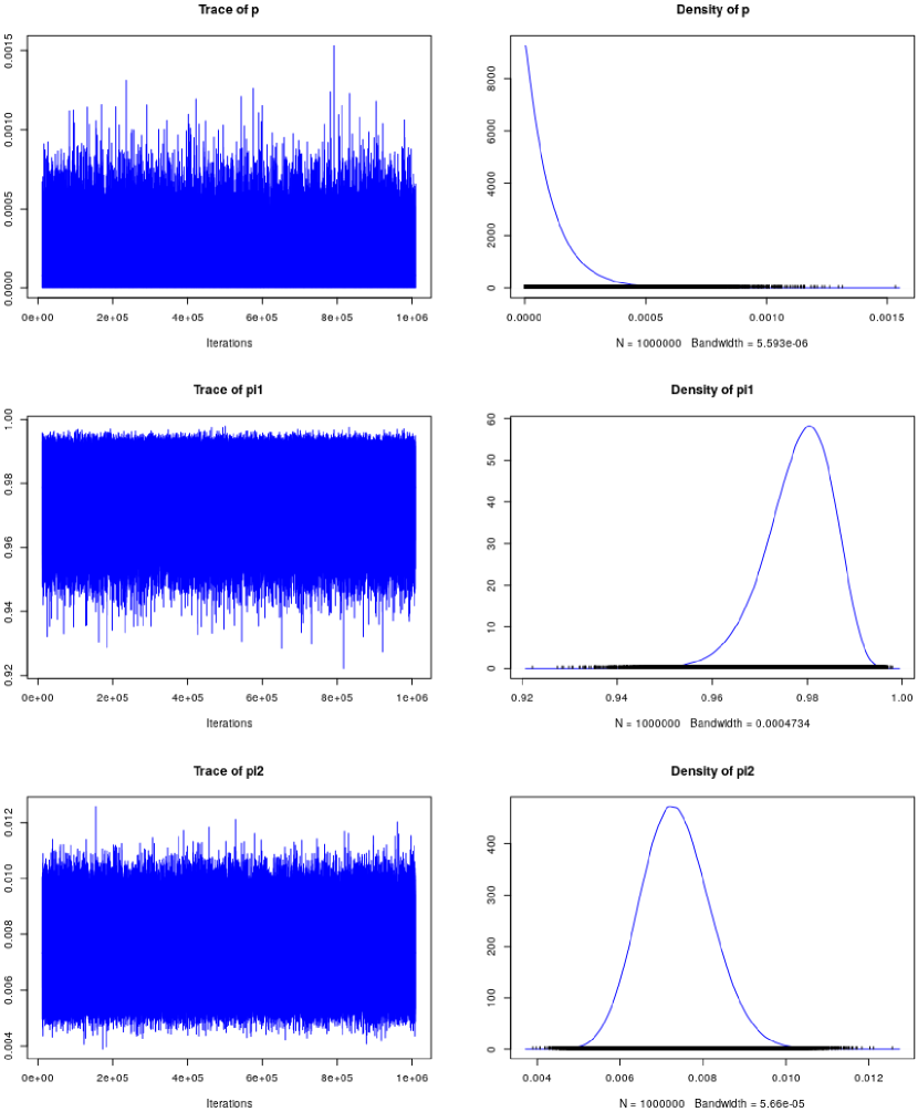
Figure 29: JAGS inference of $p$, $\pi_{1}$ and $\pi_{2}$ from $ns=10000$ and $n_{P}=50$ (see text).

and summarized as

1. Empirical mean and standard deviation for each variable,
   plus standard error of the mean:

         Mean        SD  Naive SE Time-series SE
p   0.0001022 0.0001023 1.023e-07      1.998e-07
pi1 0.9781819 0.0071445 7.145e-06      7.161e-06
pi2 0.0073581 0.0008463 8.463e-07      8.463e-07

2. Quantiles for each variable:

         2.5%       25%       50%       75%     97.5%
p   2.586e-06 2.949e-05 7.091e-05 0.0001415 0.0003771
pi1 9.622e-01 9.738e-01 9.789e-01 0.9833334 0.9899013
pi2 5.790e-03 6.771e-03 7.327e-03 0.0079113 0.0091035

As we see, the distribution of $p$ looks exponential, with mean and standard deviation practically identical and equal to $1.0\times 10^{-4}$ (we remind that it is a property of the exponential distribution to have expected value and standard deviation equal). In this case the quantiles produced by $R$ are particularly interesting, providing e.g. $P(p\leq 3.77\times 10^{-4})=97.5\%$.

The fact that a small number of infectees squeezes the distribution of $p$ towards zero follows the expectations. More surprising, at first sight, is the fact that also the value of $\pi_{2}$ does change:

$$\pi_{2}: 0.115\pm 0.022 \ \ \longrightarrow\ \ 0.0074\pm 0.0008\,.$$

The reason why $\pi_{2}$ can change (also $\pi_{1}$ could, although JAGS ‘thinks’ this is not the case) is due to the fact that it is now a unobserved node, and the $\mbox{Beta}(r_{2},s_{2})$ with which we model it is just the prior distribution we assign to it. In other words, the very small number of positives could be not only due to a very small value of $p$, but also to the possibility that $\pi_{2}$ is indeed substantially smaller than what we initially thought. This sounds absolutely reasonable, but telling exactly what the result will be can only be done using strictly the rules of probability theory, although with the help of MCMC, because in multivariate problems of this kind intuition can easily fail.

8.6 Inferring the proportions of infectees in two different populations

Let us now go through what has been anticipated in Sec. 7.4, talking about predictions. We have seen that, since (at least in our model) an important contribution to the uncertainty is due to systematics, related to the uncertain knowledge of $\pi_{1}$ and $\pi_{2}$, we cannot increase at will the sample size with the hope to reduce the uncertainty on $p$. Nevertheless, as a consequence of what we have seen in Sec. 7.4, we expect to be able to measure the difference of proportions of infectees in two populations much better than how we can measure a single proportion.

Let us use again sample sizes of 10000 (they could be different for the different populations) and imagine that we get numbers of positives rather ‘close’, as we know from the predictive distribution: $n_{P}^{(1)}=2000$ and $n_{P}^{(2)}=2200$. As far as sensitivity and specificity are concerned, since we have learned their effect, let us stick, for this exercise, to our default case, summarized by $\pi_{1}=0.978\pm 0.007$ and $\pi_{2}=0.115\pm 0.022$. The R script is given in Appendix B.11. Here is the result of the joint inference and of the difference of the proportions:

$$p^{(1)} = 0.097\pm 0.023$$

$$p^{(2)} = 0.120\pm 0.022$$

$$\Delta p=p^{(2)}-p^{(1)} = 0.023\pm 0.007$$

$$\rho(p^{(1)},p^{(2)}) = 0.955\,.$$

As we see, $p^{(1)}$ and $p^{(2)}$ are, as we use to say, ‘equal within the uncertainties’, but nevertheless their difference is rather ‘significative’. This is due to the fact that the common systematics induce a quite strong positive correlation among the determination of the two proportions, quantified by the correlation coefficient. The relevance of measuring differences has been already commented in Sec. 7.4, in which we also provided some details on how to evaluate the uncertainty of the difference from the other pieces of information. We would just like to stress its practical/economical importance. For example, dozens of regions of a state could be sampled and tested with ‘rather cheap’ kits, with performances of the kind we have seen here (but it is important that they are the same!), and only one region (or a couple of them, just for cross-checks) also with a more expensive (and hopefully more accurate) one. The region(s) tested with the high quality kit could then be used as calibration point(s) for the others and the practical impact in planning a test campaign is rather evident.

8.7 Which priors?

After having read in the first part of the paper the dramatic role of the prior, when we had to evaluate the probability of individual being infected, given the test result, one might be surprised by the regular use of a flat prior of $p$ throughout the present section. First at all, we would like to point out that we are doing so, in this case, not “in order to leave the data to ‘speak’ by themselves”, as someone says. It is, instead, the other way around: the values of $p$ preferred by the data, starting from a uniform prior, are characterized by a distribution much narrower than what we could reasonably judge, based on previous rational knowledge. In other words, they are not at odds with what we could believe independently of the data. But this is not always the case, and experts could have more precise expectation, grounded on their knowledge.

Anyway, a prior distribution is something that we have to plug in the model, if we want to perform a probabilistic inference. In practice – and let us remind again that “probability is good sense reduced to a calculus” – we model the prior in a reasonable and mathematically convenient way, and the Beta distribution is well suited for this case, also due to the flexibility of the shapes that it can assume, as seen in Sec. 4.2. Once we have opted for a Beta, a uniform prior is recovered for $r=1$ and $s=1$, although we are far from thinking that $p=0$ or $p=1$ are possible, as well as that $p$ could be above 0.9 with 10% chance, and so on.

8.7.1 Symmetric role of prior and ‘integrated likelihood’

Since we cannot go into indefinite and sterile discussions on all the possible priors that we might use (remember that if we collect and analyze data is to improve our knowledge, often used to make practical decision in a finite time scale!) it is important to understand a bit deeper their role in the inference. This can be done factorizing Eq. (82), written here in compact notation as

$$f(\ldots) = f(p,n_{I},n_{NI},n_{P_{I}},n_{P_{NI}},\pi_{1},\pi_{2},n_{P},n_{s},r_{1},s_{1},r_{2},s_{2})\,,$$ (83)

into two parts: one that only contains $f_{0}(p)$ and the other containing the remaining factors of the ‘chain’, indicated here as $f_{\emptyset}(\ldots)$:

$$f(\ldots) = f_{\emptyset}(\ldots)\cdot f_{0}(p)\,.$$ (84)

The unnormalized pdf of $p$, conditioned by data and parameters, can be then rewritten (see Appendix A) as

$$f(p\,|\,n_{P},n_{s},r_{1},s_{1},r_{2},s_{2}) \propto \left[\sum_{n_{I}}\sum_{n_{NI}}\sum_{n_{P_{I}}}\sum_{n_{P_{NI}}}\int\!\!\int\!f_{\emptyset}(\ldots)\,\mbox{d}\pi_{1}\mbox{d}\pi_{2}\right]\!\cdot f_{0}(p)\ \ \ \mbox{}$$ (85)

$$\propto {\cal L}(p\,;\,n_{P},n_{s},r_{1},s_{1},r_{2},s_{2})\cdot f_{0}(p)\,,$$ (86)

in which we have indicated with the usual symbol used for the (‘integrated’) likelihood (in which constant factors are irrelevant) the part which multiplies $f_{0}(p)$. It is then rather evident the role of ${\cal L}$ in ‘reshaping’ $f_{0}(p)$. In the particular case in which $f_{0}(p)=1$ the inference is simply given by

$$f(p\,|\,n_{P},n_{s},r_{1},s_{1},r_{2},s_{2},f_{0}(p)=1) \propto {\cal L}(p\,;\,n_{P},n_{s},r_{1},s_{1},r_{2},s_{2})$$ (87)

(“the inference is determined by the likelihood”).

If, instead, the prior is not flat, then it does reshape the posterior obtained by ${\cal L}$ alone. Therefore there are two alternative ways to see the contributions of ${\cal L}$ and $f_{0}(p)$: each one reshapes the other. In particular

• in the regions of $p$ set to zero by either function the posterior vanishes;

• the function which is more narrow around its maximum ‘wins’ against the smoother one.

Therefore, for the case shown in Fig. 26, obtained by a flat prior, the ‘density of $p$’ is nothing but the shape of ${\cal L}(p;n_{P},n_{s},r_{1},s_{1},r_{2},s_{2})$. If $f_{0}(p)$ is constant, or varies slowly, in the range $[0.02,0.17]$ it provides null or little effect. If, instead, it is very peaked around 0.15 (e.g. with a standard deviation of $\approx 0.01$) it dominates the inference.

But what is more interesting is that the reshape by $f_{0}(p)$ can be done in a second step. This is the importance of choosing a flat prior (and not just a question of laziness): the data analysis expert could then present a result of the kind of Fig. 26 to an epidemiologist who could then reshape her priors (or, equivalently, reshape the curve provided by the data analyst with her priors). But she could also have such a strong prior on the variable under study, that she could reject tout court the result, blaming the data analysis expert that there must be something wrong in the analysis or in the data – see Sec. 9.4.

8.7.2 Some examples

Let us illustrate these ideas with a simple case on which exact calculations can be also done: the inference of $p$ of a binomial distribution, based on $n$ successes got in $N$ trials. We went through it in Sec. 4, but we do it solve it now with JAGS in order to provide some details on ‘reshaping’. The model is really trivial

model {
  n ~ dbin(p, N)
  p ~ dbeta(r0,s0)
}

and the full script is provided in Appendix B.12. For $N=10$ and $n=3$ and a flat prior the JAGS result is shown by the histogram of Fig. 30.

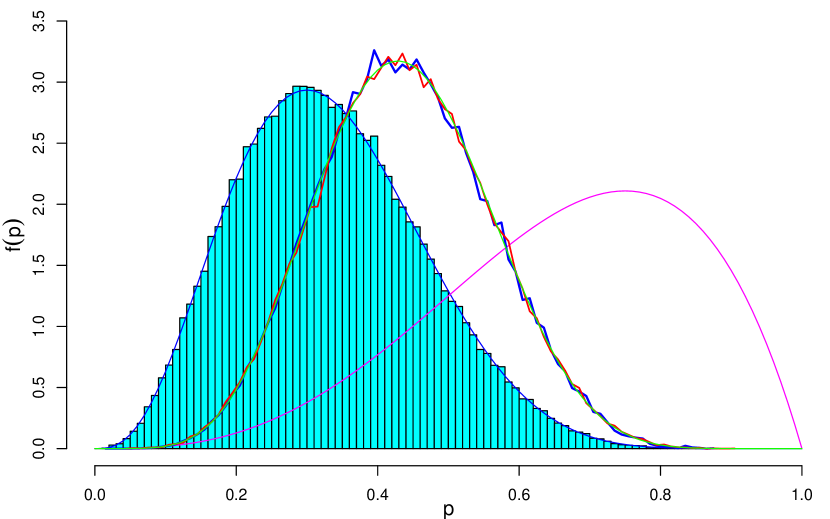
Figure 30: Inference of $p$ with binomial distributions obtained with different priors and different ways to make use of an ‘informative prior’ (see text).

The blue line along the profile of the histogram is the analytic result obtained starting from of a Beta prior with $r_{0}=s_{0}=1$, that is $\mbox{Beta}(1\!+\!n,\,1\!+\!N\!-\!n)$. Then the ‘informative prior’ (rather vague indeed), modeled by a $\mbox{Beta}(4,2)$ and therefore having a mean value of $4/(4+2)=2/3$, is shown by the magenta curve having the maximum value at $3/4\,=[(4-1)/(4+2-2)]$. The distribution obtained reweighing the posterior got from a flat prior (histogram) by this new prior is shown by the blue broken curve, while the red broken curve shows the JAGS result obtained using the new prior (the latter curves overlap so much that they can only be identified by color code). Finally, the green continuous curve is the analytic posterior obtained updating the Beta parameters, that is $\mbox{Beta}(4\!+\!3,\,2\!+\!7)$. The agreement of the three results is ‘perfect’ (taking into account that two of them are got by sampling).

The second example is our familiar case of 2010 positives in a sample of 10000 individuals shown in detail in Sec. 8.2 and of which a different Monte Carlo run, with $n_{r}=4\times 10^{6}$ in order to get a smoother histogram, is shown in Fig. 31.

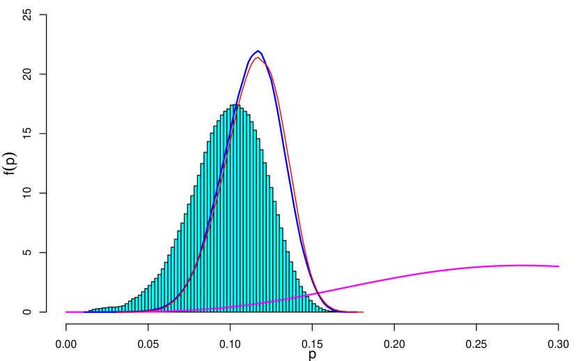
Figure 31: Inference of the proportion $p$ of infected in a population, having measured 2010 positives in a sample of 10000 individuals: JAGS result based on a flat prior (histograms) and effect of ‘reshaping’ based on an informative prior. (see text).

The new prior is indicated by the magenta curve, modeled by a $\mbox{Beta}(6,14)$, having its mode at $5/18\approx 0.28$. The reshaped posterior is indicated by the blue curve, having mean $0.1134$ and standard deviation $0.0182$. The result of JAGS using as prior the $\mbox{Beta}(6,14)$ is shown by the red curve, characterized by a mean of 0.1145 and a standard deviation 0.0184 (we are using an exaggerated number of digits just for checking – using one digit for the uncertainty both results become ‘$0.11\pm 0.02$’). The degree of agreement is excellent, also taking into account that they have intrinsic Monte Carlo fluctuations. It is interesting to note that, besides increasing slightly the mean values (but one could object that “they are equal within the uncertainties”), the main effect of the new prior is to practically rule out values of $p$ below 0.05.

8.7.3 Some approximated rules

Having seen the utility of reshaping the posterior got from a flat prior, once a different prior is assumed, we also try to find some practical rules based on the mean and the standard deviations of the distributions involved.

1. The first is based on Gaussian approximation, and it holds if both the prior and the posterior got by JAGS assuming a uniform prior appear somehow ‘bell-shaped’, although we cannot expect that they are perfectly symmetric, especially if small or large values of $p$ are preferred. In this case the following (very rough) approximation is obtained for the mean and the standard deviation

   $$\mu_{p} = \frac{\mu_{\cal L}/\sigma^{2}_{\cal L}+\mu_{0}/\sigma_{0}^{2}}{1/\sigma^{2}_{\cal L}+1/\sigma_{0}^{2}}$$ (88)

   $$\frac{1}{\sigma^{2}_{p}} = \frac{1}{\sigma^{2}_{\cal L}}+\frac{1}{\sigma_{0}^{2}}\,,$$ (89)

   where $\mu_{\cal L}$ and $\sigma_{\cal L}$ are the mean and the standard deviation got from JAGS with a flat prior; $\mu_{0}$ and $\sigma_{0}$ are those summarizing the priors; $\mu_{p}$ and $\sigma_{p}$ should be (approximately) equal to the JAGS results we had got using the prior summarized by $\mu_{0}$ and $\sigma_{0}$. Applying this rule to the case in Fig. 31, for which $\mu_{\cal L}=0.0987$, $\sigma_{\cal L}=0.0229$, $\mu_{0}=0.30$ and $\sigma_{0}=0.10$, we get $p=0.1087\pm 0.022$, that, rounding the uncertainty to one digit becomes ‘$0.11\pm 0.02$’, equal to the one obtained above by reshaping or re-running JAGS with the new prior.

2. The second rule makes use of the Beta and its usage as prior conjugate when inferring $p$ of a binomial, as we have seen in Sec. 4.2. The idea is to see the pdf estimated by JAGS with flat prior as a ‘rough Beta’ whose parameters can be estimated from the mean and the standard deviation using Eqs. (35)-(36). We can then imagine that the pdf of $p$ could have been estimated by a ‘virtual’ Poisson processes whose outcomes update the parameters of the Beta according to Eqs. (32)-(33). The trick consists then in modifying the Beta parameters according to the simple rules:

   $$r_{p} = r_{\cal L}+r_{0}-1$$

   $$s_{p} = s_{\cal L}+s_{0}-1\,,$$

   where $r_{\cal L}$ and $s_{\cal L}$ are evaluated from $\mu_{\cal L}$ and $\sigma_{\cal L}$ making use of Eqs. (35) and (36). Then the new mean and standard deviation are evaluated from $r_{p}$ and $s_{p}$ (see Sec. 4.2).

   For example, in the case of Fig. 30 we have (with an exaggerated number of digits) $p=0.0987\pm 0.0229$, which could derive from a Beta having $r_{\cal L}=16.7$ and $s_{\cal L}=152.4$. If we have a prior somehow peaked around 0.3, e.g. $p_{0}=0.3\pm 0.1$, it can be parameterized by a Beta with $r_{0}=6$ and $s_{0}=14$. Applying the above rule we get

   $$r_{p} = 16.7+6-1=21.7$$

   $$s_{p} = 152.4+14-1=165.5\,,$$

   which yield then $p=0.1159\pm 0.0223$, very similar to what was obtained by reshaping or re-running JAGS ($0.12\pm 0.02$ at two decimal digits).

As we see, these approximated rules are rather rough, but they have the advantage of being fast to apply, if one wants to arrive quickly to some reasonable conclusions, based on her personal priors.

9 Exact evaluation of $f(p)$

After having solved the inferential task by MCMC making use of JAGS, let us now attempt to solve our problem exactly, although limiting ourselves to the inference of $p$.

9.1 Setting up the problem

As we have seen in Sec. 8, the inference of the ‘unobserved’ variables, based on the ‘observed’ one, for the problem represented graphically in the ‘Bayesian’ network of Fig. 25, consists in evaluating ‘somehow’

$$f(p,n_{I},n_{NI},n_{P_{I}},n_{P_{NI}},\pi_{1},\pi_{2}\,|\,n_{P},n_{s},r_{1},s_{1},r_{2},s_{2})\,,$$ (90)

from which the most interesting probability distribution, at least for the purpose of this paper,

$$f(p\,|\,n_{P},n_{s},r_{1},s_{1},r_{2},s_{2})$$

can be obtained by marginalization (see also Appendix A). Besides a normalization factor, Eq. (90) is proportional to Eq. (82), hereafter indicated by ‘$f(\ldots)$’ for compactness, which can be written making use of the chain rule obtained following the bottom-up analysis of the graphical model of Fig. 25:

$$f(\ldots) = f(n_{P}\,|\,n_{P_{I}},n_{P_{NI}})\cdot f(n_{P_{I}}\,|\,\pi_{1},n_{I})\cdot f(n_{P_{NI}}\,|\,\pi_{2},n_{NI})\cdot f(\pi_{1}\,|\,r_{1},s_{1})\cdot$$

$$f(\pi_{2}\,|\,r_{2},s_{2})\cdot f(n_{NI}\,|\,n_{s},n_{I})\cdot f(n_{I}\,|\,p,n_{s})\cdot f_{0}(p)$$

in which

$$f(n_{P}\,|\,n_{P_{I}},n_{P_{NI}}) = \delta_{n_{p},\,n_{P_{I}}+n_{P_{NI}}}$$ (91)

$$f(n_{P_{I}}\,|\,\pi_{1},n_{I}) = \binom{n_{I}}{n_{P_{I}}}\cdot\pi_{1}^{n_{I}}\cdot(1-\pi_{1})^{n_{I}-n_{P_{I}}}$$ (92)

$$f(n_{P_{NI}}\,|\,\pi_{2},n_{NI}) = \binom{n_{NI}}{n_{P_{NI}}}\cdot\pi_{2}^{n_{P_{NI}}}\cdot(1-\pi_{2})^{n_{NI}-n_{P_{NI}`}}$$ (93)

$$f(\pi_{1}\,|\,r_{1},s_{1}) = \frac{\pi_{1}^{r_{1}-1}\cdot(1-\pi_{1})^{s_{1}-1}}{\beta(r_{1},s_{1})}$$ (94)

$$f(\pi_{2}\,|\,r_{2},s_{2}) = \frac{\pi_{2}^{r_{2}-1}\cdot(1-\pi_{2})^{s_{2}-1}}{\beta(r_{2},s_{2})}$$ (95)

$$f(n_{NI}\,|\,n_{s},n_{I}) = \delta_{n_{NI},\,n_{s}-n_{I}}$$ (96)

$$f(n_{I}\,|\,p,n_{s}) = \binom{n_{s}}{n_{I}}\cdot p^{n_{I}}\cdot(1-p)^{n_{s}-n_{I}}\,,$$ (97)

where $\delta_{m,k}$ is the Kroneker delta (all other symbols belong to the definitions of the binomial and the Beta distributions) and we have left to define the prior distribution $f_{0}(p)$. The distribution of interest is then obtained by summing up/integrating

$$f(p\,|\,n_{P},n_{s},r_{1},s_{1},r_{2},s_{2}) \propto \sum_{n_{I}}\sum_{n_{NI}}\sum_{n_{P_{I}}}\sum_{n_{P_{NI}}}\int\!\!\int\!f(\ldots)\,\mbox{d}\pi_{1}\mbox{d}\pi_{2}\,,$$

where the limits of sums and integration will be written in detail in the sequel.

As a first step we simplify the equation by summing over $n_{P_{NI}}$ and $n_{NI}$ and exploiting the Kroneker delta terms (91) and (96). We can then replace $n_{P_{NI}}$ with $n_{P}-n_{P_{I}}$ and $n_{NI}$ with $n_{s}-n_{I}$

$$f(n_{P}\!-\!n_{P_{I}}|n_{s}\!-\!n_{I},\pi_{2})\! = \!{\binom{n_{s}\!-\!n_{I}}{n_{P}\!-\!n_{P_{I}}}}\cdot{\pi_{2}}^{(n_{P}-n_{P_{I}})}\cdot(1-\pi_{2})^{(n_{s}-n_{I})-(n_{P}-n_{P_{I}})}\ \ \ \$$ (98)

with the obvious constraints $n_{s}-n_{I}>n_{P}-n_{P_{I}}$ (i.e. $n_{NI}>n_{P_{NI}}$) and $n_{P_{I}}<n_{I}$.

The inferential distribution of interest $f(p\,|\,n_{P},n_{s},r_{1},s_{1},r_{2},s_{2})$, becomes then, besides constant factors and indicating all the status of information on which the inference is based as ‘$I$’, that is $I\equiv\{n_{P},n_{s},r_{1},s_{1},r_{2},s_{2}\}$,

$$f(p\,|\,I) \propto f_{0}(p)\cdot\sum_{n_{P_{I}}=0}^{n_{P}}\sum_{n_{I}=0}^{n_{s}}\int_{0}^{1}\int_{0}^{1}\!f({n_{P_{I}}}\,|\,n_{I},\pi_{1})\cdot f(n_{P}-n_{P_{I}}|n_{s}-n_{I},\pi_{2})\cdot$$

$$f(\pi_{1}\,|\,r_{1},s_{1})\cdot f(\pi_{2}\,|\,r_{2},s_{2})\cdot f(n_{I}\,|\,p,n_{s})\,\mbox{d}\pi_{1}\,\mbox{d}\pi_{2}$$

$$\propto f_{0}(p)\cdot\sum_{n_{P_{I}}=0}^{n_{P}}\sum_{n_{I}=0}^{n_{s}}\,\int_{0}^{1}\!\int_{0}^{1}{\binom{n_{I}}{n_{P_{I}}}}\cdot{\pi_{1}}^{n_{P_{I}}}\cdot(1-\pi_{1})^{n_{I}-n_{P_{I}}}\cdot$$

$${\binom{n_{s}-n_{I}}{n_{P}-n_{P_{I}}}}\cdot{\pi_{2}}^{(n_{P}-n_{P_{I}})}\cdot(1-\pi_{2})^{(n_{s}-n_{I})-(n_{P}-n_{P_{I}})}\cdot$$

$$\pi_{1}^{r_{1}-1}\cdot(1-\pi_{1})^{s_{1}-1}\cdot\pi_{2}^{r_{2}-1}\cdot(1-\pi_{2})^{s_{2}-1}\cdot\binom{n_{s}}{n_{I}}\cdot p^{n_{I}}\cdot(1-p)^{n_{s}-n_{I}}\mbox{d}\pi_{1}\mbox{d}\pi_{2}$$

$$\propto f_{0}(p)\cdot\sum_{n_{P_{I}}=0}^{n_{P}}\sum_{n_{I}=0}^{n_{s}}\binom{n_{I}}{n_{P_{I}}}\cdot\binom{n_{s}-n_{I}}{n_{P}-n_{P_{I}}}\cdot\binom{n_{s}}{n_{I}}\!\cdot\!p^{n_{I}}\!\cdot\!(1-p)^{n_{s}-n_{I}}\cdot\!$$

$$\int_{0}^{1}\!{\pi_{1}}^{n_{P_{I}}+r_{1}-1}\cdot(1-\pi_{1})^{n_{I}-n_{P_{I}}+s_{1}-1}\,\mbox{d}\pi_{1}$$

$$\int_{0}^{1}\!{\pi_{2}}^{(n_{P}-n_{P_{I}}+r_{2}-1)}\cdot(1-\pi_{2})^{(n_{s}-n_{I})-(n_{P}-n_{P_{I}})+s_{2}-1}\,\mbox{d}\pi_{2}$$

where we have dropped all the terms not depending on the variables summed up/integrated.

The two integrals appearing in Eq. (9.1) are, in terms of the generic variable $x$, of the form $\int_{0}^{1}x^{\alpha-1}\cdot(1-x)^{\beta-1}\mbox{d}x$, which defines the special function beta $\mbox{\tt\large B}(\alpha,\beta)$, whose value can be expressed in terms of Gamma function as $\mbox{\tt\large B}(\alpha,\beta)=\Gamma(\alpha)\cdot\Gamma(\beta)/\Gamma(\alpha+\beta)$. We get then

$$f(p\,|\,I) \propto f_{0}(p)\cdot\sum_{n_{P_{I}}=0}^{n_{P}}\sum_{n_{I}=0}^{n_{s}}\left[\binom{n_{I}}{n_{P_{I}}}\cdot\binom{n_{s}-n_{I}}{n_{P}-n_{P_{I}}}\cdot\binom{n_{s}}{n_{I}}\cdot p^{n_{I}}\cdot(1-p)^{n_{s}-n_{I}}\cdot\right.$$

$$\left.\frac{\Gamma(n_{P_{I}}+r_{1})\cdot\Gamma(n_{I}-n_{P_{I}}+s_{1})}{\Gamma(r_{1}+n_{I}+s_{1})}\cdot\right.$$

$$\left.\frac{\Gamma(n_{P}-n_{P_{I}}+r_{2})\cdot\Gamma(n_{s}-n_{I}-n_{P}+n_{P_{I}}+s_{2})}{\Gamma(n_{s}-n_{I}+s_{2}+r_{2})}\right]\,.$$

9.2 Normalization factor and other moments of interest

The normalization factor $N_{f}$ is given by the integral in d$p$ of this expression, once $f_{0}(p)$ has been chosen. As we have done in the previous section, we opt for $\mbox{Beta}(r_{0},s_{0})$, taking the advantage not only of the flexibility of the probability distribution to model our ‘prior judgment’ on $p$, but also of its mathematical convenience. In fact, with this choice, the resulting term in Eq. (9.1) depending on $p$ is given by $p^{r_{0}-1+n_{I}}\cdot(1-p)^{s_{0}-1+(n_{s}-n_{I})}$. The integral over $p$ from 0 to 1 yields again a Beta function, that is $\mbox{\tt\large B}(r_{0}+n_{I},s_{0}+n_{s}-n_{I})$, thus getting

$$N_{f}\!\! = \!\!\sum_{n_{p_{I}}=0}^{n_{P}}\sum_{n_{I}=0}^{n_{s}}\left[\!\binom{n_{I}}{n_{P_{I}}}\cdot\binom{n_{s}-n_{I}}{n_{P}-n_{P_{I}}}\cdot\binom{n_{s}}{n_{I}}\cdot\frac{\Gamma(n_{P_{I}}+r_{1})\cdot\Gamma(n_{I}-n_{P_{I}}+s_{1})}{\Gamma(r_{1}+n_{I}+s_{1})}\cdot\right.$$

$$\left.\frac{\Gamma(n_{P}-n_{P_{I}}+r_{2})\cdot\Gamma(n_{s}-n_{I}-n_{P}+n_{P_{I}}+s_{2})}{\Gamma(n_{s}-n_{I}+s_{2}+r_{2})}\right.\cdot$$

$$\left.\frac{\Gamma(r_{0}+n_{I})\cdot\Gamma(s_{0}+n_{s}-n_{I})}{\Gamma(r_{0}+s_{0}+n_{s})}\right]$$

Similarly, we can evaluate the expression of the expected values of $p$ and of $p^{2}$, from which the variance follows, being $\sigma^{2}(p)=\mbox{E}(p^{2})-\mbox{E}^{2}(p)$. For example, being $\mbox{E}(p)$ given by

$$\mbox{E}(p) = \int_{0}^{1}p\cdot f(p\,|\,I)\mbox{d}p\,,$$

in the integral the term depending on $p$ becomes $p\cdot p^{r_{0}-1+n_{I}}\cdot(1-p)^{s_{0}-1+(n_{s}-n_{I})}$, increasing the power of $p$ by 1 and thus yielding

$$\mbox{E}(p)\! = \!\frac{1}{N_{f}}\cdot\sum_{n_{p_{I}}=0}^{n_{P}}\sum_{n_{I}=0}^{n_{s}}\left[\!\binom{n_{I}}{n_{P_{I}}}\!\cdot\!\binom{n_{s}-n_{I}}{n_{P}-n_{P_{I}}}\!\cdot\!\binom{n_{s}}{n_{I}}\cdot\frac{\Gamma(n_{P_{I}}+r_{1})\cdot\Gamma(n_{I}-n_{P_{I}}+s_{1})}{\Gamma(r_{1}+n_{I}+s_{1})}\right.\!\cdot$$

$$\left.\frac{\Gamma(n_{P}-n_{P_{I}}+r_{2})\cdot\Gamma(n_{s}-n_{I}-n_{P}+n_{P_{I}}+s_{2})}{\Gamma(n_{s}-n_{I}+s_{2}+r_{2})}\right.\!\cdot\!$$

$$\left.\frac{\Gamma(r_{0}+n_{I}\mbox{\boldmath$+1$})\cdot\Gamma(s_{0}+n_{s}-n_{I})}{\Gamma(r_{0}+s_{0}+n_{s}\mbox{\boldmath$+1$})}\right]\,,$$

while $\mbox{E}(p^{2})$ is obtained replacing ‘$+1$’ by ‘$+2$’. A script to evaluate expected value and standard deviation of $p$ is provided in Appendix B.13.

The expression can be extended to ‘$+3$’ by ‘$+4$’, thus getting $\mbox{E}(p^{3})$ and $\mbox{E}(p^{4})$, from which skewness and kurtosis can be evaluated. Finally, making use of the so called Pearson Distribution System implemented in R [35], $f(p)$ can be obtained with a quite high degree of accuracy, unless the distribution is squeezed towards 0 o 1, as e.g. in Fig. 29. A script to evaluate mean, variance, skewness and kurtosis, and from them $f(p)$ by the Pearson Distribution System is shown in Appendix B.14.

9.3 Result and comparison with JAGS

The pdf of $p$, given the set of conditions $I$, to which we have added $r_{0}$ and $s_{0}$ in order to remind that it also depends on the chosen family for the prior, is finally

$$f(p\,|\,I,r_{0},s_{0}) = \frac{1}{N_{f}}\cdot\Large[p^{r_{0}-1}\cdot(1-p)^{s_{0}-1}\Large]\cdot\!\sum_{n_{P_{I}}=0}^{n_{P}}\sum_{n_{I}=0}^{n_{s}}\left[\binom{n_{I}}{n_{P_{I}}}\cdot\binom{n_{s}-n_{I}}{n_{P}-n_{P_{I}}}\cdot\binom{n_{s}}{n_{I}}\cdot\right.$$

$$p^{n_{I}}\cdot(1-p)^{n_{s}-n_{I}}\cdot\frac{\Gamma(n_{P_{I}}+r_{1})\cdot\Gamma(n_{I}-n_{P_{I}}+s_{1})}{\Gamma(r_{1}+n_{I}+s_{1})}\cdot$$

$$\left.\frac{\Gamma(n_{P}-n_{P_{I}}+r_{2})\cdot\Gamma(n_{s}-n_{I}-n_{P}+n_{P_{I}}+s_{2})}{\Gamma(n_{s}-n_{I}+s_{2}+r_{2})}\right]\,.$$

So, although we have not been able to get an analytic solution, which for problems of this kind is out of hope, we have got an expression for $f(p\,|\,I,r_{0},s_{0})$, that we can compute numerically and check against the JAGS results seen in Sec. 8. For the purpose of this work, we did not put particular effort in trying to speed up the calculation of Eqs. (9.1)-(9.2) and therefore the comparison concerns only the result, and not the computer time or other technical issues. The agreement is excellent, even when we are dealing with numbers as large as 10000 for $n_{s}$ (and a few thousands for $n_{P}$). For example, the comparison using the same values of $n_{P}=2010$ and $n_{s}=10000$ of Sec. 8 is shown in the upper plot of Fig. 32:

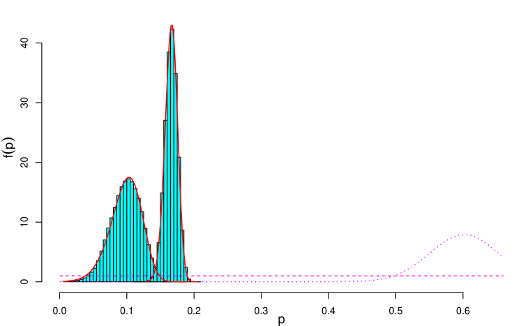
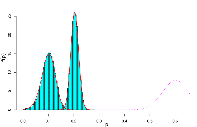
Figure 32: Direct computation of Eq. (9.3) (solid lines) vs JAGS results (histograms) for the flat prior (magenta dashed line) and for a $\mbox{Beta}(57,38)$ (magenta dotted line). Upper plot: $n_{P}=2010$ and $n_{s}=10000$. Lower plot: $n_{P}=201$ and $n_{s}=1000$.

• The histogram peaked around $p=0.1$ is the JAGS result obtained by $10^{7}$ iterations, with over-imposed the pdf evaluated making use of Eq. (9.3), starting from a uniform prior (magenta dashed line). In terms of expected value $\pm$ standard uncertainty the direct calculation (exact – see Eq. (9.2) and Appendix B.13) gives $p=0.0981\pm 0.0233$ versus $p=0.0984\pm 0.0224$ of JAGS (with exaggerated number of decimal digits just for detailed comparison).

• Then we have changed the prior, choosing one strongly preferring high values of $p$ (dotted magenta curve) with rather small uncertainty: a $\mbox{Beta}(57,38)$, yielding an expected value of 0.60 with standard deviation of 0.05. This new prior has the effect of ‘pulling’ the distribution of $p$ on the right side. The agreement of the results obtained by the two methods is again excellent, resulting in $p=0.1669\pm 0.0093$ and $p=0.01658\pm 0.0093$ (direct and JAGS, respectively).

Then we repeat the game with a sample ten times smaller, that is $n_{s}=1000$, and assuming $n_{P}=201$ (lower plot in the same figure). Again the agreement between direct calculation and MCMC sampling is excellent.

It is worth noting that the possibility to write down an expression for the pdf of interest for an inferential problem with several nodes, after marginalization over six variables, has to be considered a lucky case, thanks also to the approximation of modeling the sampling by a binomial rather than a hypergeometric and to the use of conjugate priors. The purpose of this section is then mainly didactic, being the valuation of the pdf’s of other variables (and of several variables all together) and of their moments prohibitive. It is then clear the superiority of estimates based on MCMC methods, whose advent several decades ago has been a kind of revolution, which have given a boost to Bayesian methods for ‘serious’ multidimensional applications, tasks before not even imaginable.

9.4 More remarks on the role of priors

Having checked the agreement between the two methods, let us now focus the attention on the results themselves. Looking at the results from the smaller sample we note:

• The width of the distribution using a flat prior is wider for the small sample than that obtained with larger ‘statistics’, as expected, with a tiny variation in the mean value: $p=0.099\pm 0.027$.

• The prior $\mbox{Beta}(57,38)$ causes a larger shift of the distribution towards higher values of $p$, thus yielding $p=0.204\pm 0.015$.

It is interesting to compare these results with what we have seen in Sec. 8.7 (see Fig. 31). In that case the non-flat, ‘informative’ prior had the role of ‘reshaping’ the posterior derived by a flat prior, making thus the result acceptable by the ‘expert’, because the outcome was not in contrast with her prior belief. Here, instead, the result provided by a flat prior is so far from the rational belief (most likely shared by the relevant scientific community) of the expert, that the result would not be accepted acritically. Most likely the expert would mistrust the data analysis, or the data themselves. But she would perhaps also analyze critically her prior beliefs in order to understand on what they were really grounded and how solid they were. As a matter of fact, scientists are ready to modify their opinion, but with some care, and, as the famous motto says, “extraordinary claims require extraordinary evidence”.

Since scientific priors are usually strongly based on previous experimental information, the problem of ‘logically merging’ a prior preference summarized by $\approx 0.60\pm 0.05$ and a new experimental results preferring ‘by itself’ (that is when the result is dominated by the ‘likelihood’ – see Sec. 8.7), summarized as $0.098\pm 0.023$ (or $\pm 0.027$, depending on $n_{s}$) is similar to that of ‘combining apparently incompatible results.’ Also in that case, nobody would acritically accept the ‘weighted average’ of the two results which appear to be in mutual disagreement. A so called ‘skeptical combination’ should be preferred, which would even yield a multi-modal distribution [34]. This means that in a case like those of Fig. 32 the expert could think that either

• she is right, with probability ${\cal P}$, and she would just stick to her prior $f_{0}(p)$;

• she is wrong, with probability $1-{\cal P}$, and she would switch to the posterior provided by the likelihood alone, let us indicate it with $f_{\cal L}(p)$.

Therefore the degrees of belief of $p$ will be described by $f(p)={\cal P}\cdot f_{0}(p)+(1-{\cal P})\cdot f_{\cal L}(p)$. As far as we understand from our experience she would hardly believe the result obtained, ‘technically’, plugging her prior in the formulae – and we keep repeating once more Laplace’s dictum that “probability is good sense reduced to a calculus”.

In order to make our point more clear, let us look into the details of the situation depicted in Fig. 32 with the help of Fig. 33, in which

Figure 33: Closer look at the effect of the prior $\mbox{Beta}(57,38)$ shown in Fig. 32.

$f(p)$ is reported in log scale, and the abscissa limited to the region of interest. The blue curves, which are dominant below $p\approx 0.10$, represent the posteriors obtained by a flat prior (solid for $n_{s}=10000$ and $n_{P}=2010$; dashed for $n_{s}=1000$ and $n_{P}=201$). Then, the dotted magenta curve is the tail at small $p$ of the prior $\mbox{Beta}(57,58)$, which prefers values of $p$ around $\approx 0.60\pm 0.05$. Then the red curves (solid and dashed as previously) show the posterior distributions obtained by this new prior.

The shift of both distributions towards the right side is caused by the dramatic reshaping due to prior in the region between $p\approx 0.1$ and $p\approx 0.3$ in which $f_{0}(p\,|\,\mbox{Beta}(57,38))$ varies by about 25 orders of magnitudes (!). The question is then that no expert, who believes a priori that $p$ should be most likely in the region between 0.5 and 0.7 (and almost certainly not below 0.40-0.45), can have a defensible, rational belief that values of $p$ around 0.3 are $10^{\approx 25}$ times more probable than values around 0.1. More likely, once she has to give up her prior, she would consider small values of $p$ equally likely. For this reason – let us put in this way what we have said just above – she will be in the situation either to completely mistrust the new outcome, thus keeping her prior, or the other way around. The take-away message is therefore just the (trivial) reminder that mathematical models are in most practical cases just dictated by practical convenience and should not been taken literally in their extreme consequences, as Gauss promptly commented on the “defect” of his error function immediately after he had derived it [30]. Therefore our addendum to Laplace’s dictum reminded above is don’t get fooled by math.

10 Conclusions

In this paper we went through the issues of ‘stating’ if an individual belong to a particular class and in ‘counting’ the number of individuals in a population belonging to that class. Since the casus belli was the Covid-19 pandemic, we have been constantly speaking of (currently and past) ‘infectees’, although our work is rather general. A well understood complication related to the above tasks is due to the fact that the assignment of an individual to the class of interest is performed by ’proxies’ provided by the test result, in this case ‘positive’ or ‘negative’. Having defined $\pi_{1}$ the probability that the test result gives positive if the individual is infected (‘sensitivity’) and $\pi_{2}$ the probability of positive if not infected ($1-\pi_{2}$ being the ‘specificity’), we have analyzed the impact on the results of the fact that not only these ‘test parameters’ are far from being ideal ($\pi_{1}\neq 1$ and $\pi_{2}\neq 0$), but that their values are indeed uncertain.

We have started our work using parameters that can be summarized as $\pi_{1}=0.978\pm 0.007$ and $\pi_{2}=0.115\pm 0.022$, based on the nominal data provided by Ref. [2] ($\pi_{1}=0.98$ and $\pi_{2}=0.12$), and used probability theory, and in particular the so called Bayes’ rule, in order to

• evaluate the probability that an individual declared positive is infected (and so on for the other possibilities);

• evaluate the proportion of infectees in a population, based on the number of positive in a tested sample.

In both problems the role of ‘priors’ is logically crucial, although in practice it has a different impact on the numerical result:

• the probability that an individual tagged as positive is infected depends strongly on the probability of being infected based on other pieces of information and knowledge (in the idealistic case of ‘zero knowledge’ this prior probability is just the assumed proportion of infectees in the population);

• the probability density function of the proportion of infectees in the population has, instead, usually a weak dependence on the prior beliefs about the same proportion.

The dependence on the fact that the tests are ‘imperfect’ has a different impact on the result:

• the probability of infected if positive depends strongly, as expected, on the values (‘expected values’, in probabilistic terms) of $\pi_{1}$ and $\pi_{2}$, while, rather surprisingly, it depends very little on their uncertainty;

• the inference of the proportion of infectees, instead, depends strongly on their uncertainty, but very little on their expected values.

The latter outcome is important for planning test campaigns to count and regularly monitor the number of infectees in a population, for which tests with relatively low sensitivity and specificity can be employed. This second task has been analyzed in detail by exact evaluations, Monte Carlo methods and approximated formulae, first to understand the accuracy of the predictions of the number of positives that would result in a sample of the population, assuming a given proportion of infectees in the population; then to infer the proportion of infectees in the population from the observed number of positives.

The preliminary work of predicting the number of positives has been particularly important because it has allowed us to produce approximated formulae with which we can disentangle the contributions to the overall uncertainty of prediction, which has a somehow specular relation with the uncertainty in inference. This allows to classify then the contributions into ’statistics’ (those depending on the sample size, due to the probabilistic effects of sampling) and ‘systematics’ (those not depending on the sample size, due then to the uncertainties on $\pi_{1}$ and $\pi_{2}$). As a consequence it is possible to evaluate the critical sample size, above which uncertainties due to systematics are dominant, and therefore it is not worth increasing the sample size.

Moreover, the fact that the uncertainties about $\pi_{1}$ and $\pi_{2}$ act as systematics (within the limitation of our model, clearly stated in Sec. 5.2) suggests that we can evaluate differences of proportions of infectees in different populations much better than how we can measure a single proportion. This observation has an important practical consequence, because one could measure the proportion of infectees in a subpopulation (think e.g. to a Region of a Country) both with a test of higher quality (and presumably more expensive) and with a cheaper, rapid and less accurate one and therefore use the result as calibration point for the other subpopulations.

Appendix A – Some remarks on ‘Bayes’ formulae’

Equation (6) is a straight consequence of the probability rule relating joint probability to conditional probability, that is, for the generic ‘events’ $A$ and $B$,

$$P(A\cap B) = P(B\,|\,A)\cdot P(A)=P(A\,|\,B)\cdot P(B)\,,\hskip 65.44142pt\,\mbox{(A.1)}$$

having added to $P(\mbox{Inf})$ of Eq. (6) the suffix ‘0’ in order to emphasize its role of ‘prior’ probability. Equation (A.1) yields trivially

$$P(A\,|\,B) = \frac{P(B\,|\,A)\cdot P(A)}{P(B)}\ \ \longrightarrow\ \ \frac{P(B\,|\,A)\cdot P_{0}(A)}{P(B)}\,,\hskip 42.67912pt\,\mbox{(A.2)}$$

having also emphasized that $P(A)$ in r.h.s. is the probability of $A$ before it is updated by the new condition $B$. But, indeed, the essence of the Bayes’ rule is given by

$$P(A\,|\,B) = \frac{P(A\cap B)}{P(B)}=\frac{P(A,B)}{P(B)}\,,\hskip 139.41832pt\,\mbox{(A.3)}$$

in which we have rewritten the ‘$A\cap B$’ in the way it is custom for uncertain numbers (‘random variables’), as we shall see in while. Moreover, as we can ‘expand’ the numerator (using the so called chain rule) to go from Eq. (A.3) to Eq. (A.2), and then Eq. (6), similarly we can expand the denominator in two steps. We start ‘decomposing’ $B$ into $B\cap A$ and $B\cap\overline{A}$, from which it follows

$$B = (B\cap A)\cup(B\cap\overline{A})$$

$$P(B) = P(B\cap A)+P(B\cap\overline{A})$$

$$= P(B\,|\,A)\cdot P(A)+P(B\,|\,\overline{A})\cdot P(\overline{A})$$

After the various ‘expansions’ we can rewrite Eq. (A.3) as

$$P(A\,|\,B) = \frac{P(B\,|\,A)\cdot P(A)}{P(B\,|\,A)\cdot P(A)+P(B\,|\,\overline{A})\cdot P(\overline{A})}\,.\hskip 76.82234pt\,\mbox{(A.4)}$$

Finally, if instead of only two possibilities $A$ and $\overline{A}$, we have a complete class of hypotheses $H_{i}$, i.e. such that $\sum_{i}P(H_{i})=1$ and $P(H_{i}\cap H_{j})=0$ for $i\neq j$, we get the famous

$$P(H_{i}\,|\,E) = \frac{P(E\,|\,H_{i})\cdot P(H_{i})}{\sum_{i}P(E\,|\,H_{i})\cdot P(H_{i})}\ \ \ \longleftarrow\ \ \frac{P(H_{i}\cap E)}{P(E)}\,,\hskip 36.98866pt\,\mbox{(A.5)}$$

having also replaced the symbol $B$ by $E$, given its meaning of effect, upon which the probabilities of the different hypotheses $H_{i}$ are updated. Moreover, the sum in the denominator of the first r.h.s. of Eq. (A.5) makes it explicit that the denominator is just a normalization factor, and therefore the essence of the reasoning can be expressed as

$$P(H_{i}\,|\,E) \propto P(E\,|\,H_{i})\cdot P(H_{i})=P(H_{i}\cap E)\hskip 96.73918pt\,\mbox{(A.6)}$$

The extension to discrete ‘random variables’ is straightforward, since the probability distribution $f(x)$ has the meaning of $P(X=x)$, with $X$ the name of the variable and $x$ one of the possible values that it can assume. Similarly, $f(x,y)$ stands for $P(X=x,Y=y)\equiv P\left((X=x)\cap(Y=y)\right)$, $f(x\,|\,y)$ for $P(X=x\,|\,Y=y)$, and so on. Moreover all possible values of $X$, as well as all possible values of $Y$, form a complete class of hypotheses (the distributions are normalized). Equation (A.3) and its variations and ‘expansions’ becomes then, for $X$ and $Y$,

$$f(x\,|\,y) = \frac{f(x,y)}{f(y)}=\frac{f(y\,|\,x)\cdot f(x)}{f(y)}=\frac{f(y\,|\,x)\cdot f(x)}{\sum_{x}f(y,x)}=\frac{f(y\,|\,x)\cdot f(x)}{\sum_{x}f(y\,|\,x)\cdot f(x)}\hskip 17.07182pt$$

$$\propto f(y\,|\,x)\cdot f(x)=f(x,y)\,,\hskip 207.7052pt\,\mbox{(A.7)}$$

which can be further extended to several other variables. For example, adding $Z$, $V$ and $W$ and being interested to the joint probability that $X$ and $Z$ assume the values $x$ and $z$, conditioned by $Y=y$, $V=v$ and $W=w$, we get

$$f(x,z\,|\,y,v,w) = \frac{f(x,y,v,w,z)}{f(y,v,w)}\,.\hskip 153.6447pt\,\mbox{(A.8)}$$

To conclude, some remarks are important, especially for the applications:

1. Equations (A.7) and (A.8) are valid also for continuous variables, in which case the various ‘$f()$’ have the meaning of probability density function, and the sums needed to get the (possibly joint) marginal in the denominator are replaced by integration.

2. The numerator of Eq. (8) is ‘expanded’ using a chain rule, choosing, among the several possibilities, that which makes explicit the (assumed) causal connections of the different variables in the game, as stressed in the proper places through the paper (see e.g. footnote 15, Sec. 7 and Sec. 9).

3. A related remark is that, among the variables entering the game, as those of Eq. (A.8), some may be continuous and other discrete and the probabilistic meaning of ‘$f(\ldots)$’, taking the example of a bivariate case $f(x,y)$ with $x$ discrete and $y$ continuous, is given by $P(X=x,y\leq Y\leq y+\mbox{d}y)=f(x,y)\,\mbox{d}y$, with the normalization condition given by $\sum_{x}\int f(x,y)\,\mbox{d}y=1$.

4. Finally, a crucial observation is that, given the model which connects the variables (the graphical representations of the kinds shown in the paper are very useful to understand it) and its parameters, the denominator of Eq. (A.8) is just a number (although often very difficult to evaluate!), and therefore, as we have seen in Eq. (A.7), the last equation can be rewritten as^(∗)

   $$f(x,z\,|\,y,v,w) \propto f(x,y,v,w,z)\,,\hskip 153.6447pt\,\mbox{(A.9)}$$

   
   or, denoting by $\tilde{f}()$ the un-normalized posterior distribution,

   $$\tilde{f}(x,z\,|\,y,v,w) = f(x,y,v,w,z)\,.\hskip 153.6447pt\,\mbox{(A.10)}$$

   The importance of this remark is that, although a closed form of posterior is often prohibitive in practical cases, an approximation of it can be obtained by Monte Carlo techniques, which allow us to evaluate the quantities of interest, like averages, probability intervals, and so on (see references in footnote 40).

——————————————————————————————————
^(∗) Perhaps a better way to rewrite (A.9) and (A.10), in order to avoid confusion, could be

$$f(x,z\,|\,y=y_{0},v=v_{0},w=w_{0}) \propto f(x,y_{0},v_{0},w_{0},z)$$

$$\tilde{f}(x,z\,|\,y=y_{0},v=v_{0},w=w_{0}) = f(x,y_{0},v_{0},w_{0},z)\,,$$

in order to emphasize the fact that $y$, $v$ and $w$ assume precise values, under which the possible values of $x$ and $z$ are conditioned. Anyway, it is just a question of getting used with that notation. For example, sticking to a textbook two dimensional case, the bivariate normal distribution is given by

$$f(x,y)\! = \!\frac{1}{2\,\pi\,\sigma_{x}\,\sigma_{y}\,\sqrt{1-\rho^{2}}}\,\exp\left\{-\frac{1}{2\,(1-\rho^{2})}\left[\frac{(x-\mu_{x})^{2}}{\sigma_{x}^{2}}-2\,\rho\,\frac{(x-\mu_{x})(y-\mu_{y})}{\sigma_{x}\,\sigma_{y}}+\frac{(y-\mu_{y})^{2}}{\sigma_{y}^{2}}\right]\right\}\,.$$

The distribution of $x$, conditioned by $y=y_{0}$ is then

$$f(x\,|\,y_{0})\! \propto \!\frac{1}{2\,\pi\,\sigma_{x}\,\sigma_{y}\,\sqrt{1-\rho^{2}}}\,\exp\left\{-\frac{1}{2\,(1-\rho^{2})}\left[\frac{(x-\mu_{x})^{2}}{\sigma_{x}^{2}}-2\,\rho\,\frac{(x-\mu_{x})(y_{0}-\mu_{y})}{\sigma_{x}\,\sigma_{y}}+\frac{(y_{0}-\mu_{y})^{2}}{\sigma_{y}^{2}}\right]\right\}$$

$$\propto \!\exp\left\{-\frac{1}{2\,(1-\rho^{2})}\left[\frac{(x-\mu_{x})^{2}}{\sigma_{x}^{2}}-2\,\rho\,\frac{x\,(y_{0}-\mu_{y})}{\sigma_{x}\,\sigma_{y}}\right]\right\}$$

$$\propto \!\exp\left\{-\frac{1}{2\,(1-\rho^{2})\,\sigma_{x}^{2}}\left[x^{2}-2\,x\,\left(\mu_{x}+\rho\frac{\sigma_{x}}{\sigma_{y}}\,(y_{0}-\mu_{y})\right)\right]\right\}$$

$$\propto \!\exp\left\{-\frac{\left[x^{2}-2\,x\,\left(\mu_{x}+\rho\frac{\sigma_{x}}{\sigma_{y}}\,(y_{0}-\mu_{y})\right)\right]}{2\,(1-\rho^{2})\,\sigma_{x}^{2}}\right\}$$

$$\propto \exp\left\{-\frac{\left[x-\,\left(\mu_{x}+\rho\frac{\sigma_{x}}{\sigma_{y}}\,(y_{0}-\mu_{y})\right)\right]^{2}}{2\,(1-\rho^{2})\,\sigma_{x}^{2}}\right\}\,,$$

in which we recognize a Gaussian distribution with $\mu_{x|y_{0}}=x+\rho\frac{\sigma_{x}}{\sigma_{y}}\,(y_{0}-\mu_{y})$ and $\sigma_{x|y_{0}}=\sqrt{1-\rho^{2}}\,\sigma_{x}$.
$[$In the various steps all factors (and hence all addends at the exponent) not depending on $x$ have been ignored. Finally, in the last step the ‘trick’ of complementing the exponential has been used, because adding $\left(\mu_{x}+\rho\frac{\sigma_{x}}{\sigma_{y}}\,(y_{0}-\mu_{y})\right)^{2}\!/\,(2\,(1-\rho^{2})\,\sigma_{x}^{2})$ at the exponent is the same as multiplying by a constant factor.$]$

Appendix B – R and JAGS code

B.1 – Monte Carlo evaluation of Eqs. (41) and (42)

r.pi1 = 409.1; s.pi1 = 9.1
r.pi2 =  25.1; s.pi2 = 193.1
p = 0.1
n = 100000
pi1 <- rbeta(n, r.pi1, s.pi1)
pi2 <- rbeta(n, r.pi2, s.pi2)
P.Inf.Pos.i   <-  pi1*p/(pi1*p + pi2*(1-p))
P.NoInf.Neg.i <- (1-pi2)*(1-p) / ((1-pi1)*p + (1-pi2)*(1-p))
P.Inf.Pos   <- mean(P.Inf.Pos.i)
P.NoInf.Neg <- mean(P.NoInf.Neg.i)
cat(sprintf("Integral (by MC): P(Inf|Pos) = %.4f; P(NoInf|Neg) = %.4f \n",
            P.Inf.Pos, P.NoInf.Neg))
E.pi1 = r.pi1 / (r.pi1 + s.pi1)
E.pi2 = r.pi2 / (r.pi2 + s.pi2)
cat(sprintf("Using E(..): P(Inf|Pos) = %.4f;  P(NoInf|Neg) = %.4f \n",
            E.pi1*p/(E.pi1*p + E.pi2*(1-p)),
            (1-E.pi2)*(1-p) / ((1-E.pi1)*p + (1-E.pi2)*(1-p))))

B.2 – Monte Carlo evaluation of Eq. (50)

ns = 10000
ps = 0.1
n.I = ps * ns
n.NI = (1 - ps) * ns
r1=409.1; s1=9.1
r2=25.1; s2=193.2
nr =100000
pi1 <- rbeta(nr, r1, s1)
pi2 <- rbeta(nr, r2, s2)
nP.I  <- rbinom(nr, n.I, pi1)
nP.NI <- rbinom(nr, n.NI, pi2)
nP <- nP.I + nP.NI
hist(nP, nc=100, col=’cyan’, freq=FALSE)
cat(sprintf("nP: mean = %.1f, sd = %.1f\n",mean(nP),sd(nP)))

B.3 – Monte Carlo estimate of $f(n_{P}\,|\,N=10^{5},n_{s}=10^{4},p=0.1)$ reported in Fig. 12

N = 100000; ns  = 10000; p = 0.1
N.I  <- as.integer(p*N)
N.NI <- N - N.I
E.pi1 = 0.978; E.pi2 = 0.115

nr =100000
n.I  <- rhyper(nr, m=N.I, n=N.NI, k=ns)
n.NI <- ns - n.I

nP.I  <- rbinom(nr, n.I, E.pi1)
nP.NI <- rbinom(nr, n.NI, E.pi2)
nP <- nP.I + nP.NI
cat(sprintf("mean = %.0f,  sigma = %.0f\n", mean(nP),  sd(nP) ))
hist(nP, nc=90, col=’cyan’, freq=FALSE)

B.4 – $\sigma(f_{P})$ and $\sigma(f_{P})/\mbox{\rm E}(f_{P})$, with detailed contributions to them, using the approximated Eqs. (71)-(76)

p  = 0.1
N  = 10^7    # N >> ns --> binomial
ns = 1000
E.pi1 = 0.978;  sigma.pi1 = 0.007
E.pi2 = 0.115;  sigma.pi2 = 0.022
# E.pi2 = 0.115;  sigma.pi2 = sigma.pi1     # reduced sigma.pi2
# E.pi2 = 1 - E.pi1; sigma.pi2 = sigma.pi1  # improved specificity

E.ps <- p
E.fP <- E.pi1*E.ps + E.pi2*(1-E.ps)

s.fP.R   <- sqrt( E.pi1*(1-E.pi1)*E.ps +  E.pi2*(1-E.pi2)*(1-E.ps) )/sqrt(ns)
s.fP.pi1 <- sigma.pi1*E.ps
s.fP.pi2 <- sigma.pi2*(1-E.ps)
s.ps     <- sqrt(p*(1-p)*(1-ns/N))/sqrt(ns)
s.fP.ps  <- s.ps*abs(E.pi1-E.pi2)

s.fP.stat <- sqrt(s.fP.R^2+s.fP.ps^2)
s.fP.syst <- sqrt(s.fP.pi1^2+s.fP.pi2^2)
s.fP = sqrt(s.fP.stat^2 + s.fP.syst^2)

cat(sprintf("p = %.2f; ns = %d\n", p, ns))
cat(sprintf("E(fN) = %.3f; sigma(fN) = %.3f; sigma(fN)/E(fN) = %.2f\n",
            E.fP, s.fP, s.fP/E.fP))
cat("Contributions : \n")
cat(sprintf("    s.fP.R    =  %.3e;  s.fP.R/E.fP    = %.2e\n",
            s.fP.R, s.fP.R/E.fP))
cat(sprintf("    s.fP.p1   =  %.3e;  s.fP.p1/E.fP   = %.2e\n",
            s.fP.pi1, s.fP.pi1/E.fP))
cat(sprintf("    s.fP.p2   =  %.3e;  s.fP.p2/E.fP   = %.2e\n",
            s.fP.pi2, s.fP.pi2/E.fP))
cat(sprintf("    s.fP.ps   =  %.3e;  s.fP.ps/E.fP   = %.2e\n",
            s.fP.ps, s.fP.ps/E.fP))
cat(sprintf("    s.fP.stat =  %.3e;  s.fP.stat/E.fP = %.2e\n",
            s.fP.stat, s.fP.stat/E.fP))
cat(sprintf("    s.fP.syst =  %.3e;  s.fP.syst/E.fP = %.2e\n",
            s.fP.syst, s.fP.syst/E.fP))

B.5 – Monte Carlo estimate of $f_{P}$ using R functions, as described in Sec. 7.2.1 (see Fig.21)

p  = 0.1
ns = 1000
r1 = 409.1;  s1 =  9.1
r2 =  25.1;  s2 =193.2

nr = 10000
n.I   <- rbinom(nr, ns, p)       # 1.
n.NI  <- ns - n.I
pi1   <- rbeta(nr, r1, s1)       # 2.
pi2   <- rbeta(nr, r2, s2)
nP.I  <- rbinom(nr, n.I, pi1)    # 3.
nP.NI <- rbinom(nr, n.NI, pi2)
nP    <- nP.I + nP.NI            # 4.

fP <- nP/ns
cat(sprintf("fP: %.3f +- %.3f\n", mean(fP), sd(fP)))
hist(fP, col=’cyan’)
# barplot(table(fP), col=’cyan’)  # alternative, for small ns and p

B.6 – Monte Carlo estimate of $f_{P}$ JAGS from R via rjags (Sec. 7.2.2)

#--------------------------  JAGS model ------------------------------
model.name = "tmp_model.bug"
write("
model {
  n.I ~ dbin(p, ns)
  n.NI <- ns - n.I
  nP.I ~ dbin(pi1, n.I)
  nP.NI ~ dbin(pi2, n.NI)
  pi1 ~ dbeta(r1, s1)
  pi2 ~ dbeta(r2, s2)
  nP ~ sum(nP.I, nP.NI)
  fP <- nP / ns
}
", model)

#--------------------------- call JAGS ---------------------------------
library(rjags)
data <- list(ns=1000, p=0.1, r1=409.1, s1=9.1, r2=25.2, s2=193.1)
jm <- jags.model(model, data)
chain <- coda.samples(jm, c(’n.I’, ’fP’), n.iter=10000)

#--------------------------- Results ------------------------------------
print(summary(chain))
plot(chain, col=’blue’)

B.7 – Check of approximated formulae

get.prediction <- function(ns, N, p, E.pi1, sigma.pi1, E.pi2, sigma.pi2) {
   E.ps <- p
   E.fP <- E.pi1*E.ps + E.pi2*(1-E.ps)

   s.fP.R   <- sqrt( E.pi1*(1-E.pi1)*E.ps +  E.pi2*(1-E.pi2)*(1-E.ps) )/sqrt(ns)
   s.fP.pi1 <- sigma.pi1*E.ps
   s.fP.pi2 <- sigma.pi2*(1-E.ps)
   s.ps     <- sqrt(p*(1-p)*(1-ns/N))/sqrt(ns)
   s.fP.ps  <- s.ps*abs(E.pi1-E.pi2)

   s.fP.stat <- sqrt(s.fP.R^2+s.fP.ps^2)
   s.fP.syst <- sqrt(s.fP.pi1^2+s.fP.pi2^2)
   s.fP = sqrt(s.fP.stat^2 + s.fP.syst^2)
   return(list(E.fP=E.fP, s.fP=s.fP))
}

N  = 10^7
p.v  <- 0:4 / 10
ns.v <- c(300, 1000, 3000, 10000)

E.pi1 = 0.978;  sigma.pi1 = 0.007
E.pi2 = 0.115;  sigma.pi2 = 0.022
for(case in 1:3) {
  if(case == 2) sigma.pi2 = sigma.pi1
  if(case == 3) E.pi2 = 1 - E.pi1
  cat(sprintf("\n [pi1 = %.3f+-%.3f;", E.pi1, sigma.pi1))
  cat(sprintf(" pi2 = %.3f+-%.3f]\n", E.pi2, sigma.pi2))
  for(i in 1:length(ns.v)) {
    ns <- ns.v[i]
    cat(sprintf(" ns = %d\n p: ", ns))
    for(j in 1:length(p.v))  cat(sprintf("   %.2f      ", p.v[j]))
    cat("\nfP: ")
    for(j in 1:length(p.v)) {
     p <- p.v[j]
      pred <- get.prediction(ns, N, p, E.pi1, sigma.pi1, E.pi2, sigma.pi2)
     cat(sprintf("%.3f+-%.3f ", pred$E.fP, pred$s.fP))
    }
    cat("\n")
  }
}

B.8 – Predicting the fractions of positives obtained sampling two different populations (Sec. 7.4)

get.fP  <- function(nr, p, ns, pi1, pi2) {
  n.I   <- rbinom(nr, ns, p)
  n.NI  <- ns - n.I
  nP.I  <- rbinom(nr, n.I, pi1)
  nP.NI <- rbinom(nr, n.NI, pi2)
  nP    <- nP.I + nP.NI
  fP    <- nP/ns
  return(fP)
}

p1 = 0.1
p2 = 0.2
ns = 10000
r1 = 409.1;  s1 =  9.1
r2 =  25.1;  s2 =193.2

nr = 100000
pi1 <- rbeta(nr, r1, s1)
pi2 <- rbeta(nr, r2, s2)
fP1 <- get.fP(nr, p1, ns, pi1, pi2)
fP2 <- get.fP(nr, p2, ns, pi1, pi2)

cat(sprintf("fP1: %.4f +- %.4f\n", mean(fP1), sd(fP1)))
cat(sprintf("fP2: %.4f +- %.4f\n", mean(fP2), sd(fP2)))
cat(sprintf("fP2-fP1: %.4f +- %.4f\n", mean(fP2-fP1), sd(fP2-fP1)))
cat(sprintf("rho(fP1,fP2): %.4f\n", cor(fP1,fP2)))
cat(sprintf("Check of sigma(fP2-fP1) from correlation: %.4f\n",
            sqrt(var(fP1)+var(fP2)-2*cov(fP1,fP2))))

(Note how the ‘random’ sequences of values of pi1 and pi2 are generated before the calls to get.fP(). This is crucial in order to get the correlation among fP1 and fP2 discussed in Sec. 7.4. If these two sequences are defined, each time, inside the function, or they a generated before each call to the function, the correlation will disappear. This way of generating the events is consequence of our model assumptions, as stressed in Sec. 5.2.)

B.9 – JAGS model to perform the same Monte Carlo evaluation done in Appendix B.8

(Only the model is provided – steering R commands are left as exercise.)

model {
  n.I.1 ~ dbin(p1, ns1)
  n.NI.1 <- ns1 - n.I.1
  nP.I.1 ~ dbin(pi1, n.I.1)
  nP.NI.1 ~ dbin(pi2, n.NI.1)
  nP.1 ~ sum(nP.I.1, nP.NI.1)
  fP.1 <- nP.1 / ns1

  n.I.2 ~ dbin(p2, ns2)
  n.NI.2 <- ns2 - n.I.2
  nP.I.2 ~ dbin(pi1, n.I.2)
  nP.NI.2 ~ dbin(pi2, n.NI.2)
  nP.2 ~ sum(nP.I.2, nP.NI.2)
  fP.2 <- nP.2 / ns2

  D.fP <- fP.2 - fP.1

  pi1 ~ dbeta(r1, s1)
  pi2 ~ dbeta(r2, s2)
}

B.10 – JAGS model to infer $p$ (see Sec. 8.2)

#---- data and parameters
nr = 1000000
ns = 10000
nP = 2010
r0 = s0 = 1
r1 = 409.1; s1 = 9.1
r2 = 25.2;  s2 = 193.1

#---- JAGS model ------------------------------
model = "tmp_model.bug"    # name of the model file (’temporary’)
write("
model {
  nP ~ sum(nP.I, nP.NI)
  nP.I ~ dbin(pi1, n.I)
  nP.NI ~ dbin(pi2, n.NI)
  pi1 ~ dbeta(r1, s1)
  pi2 ~ dbeta(r2, s2)
  n.I ~ dbin(p, ns)
  n.NI <- ns - n.I
  p ~ dbeta(r0,s0)
}
", model)

#---- call JAGS ---------------------------------------------
library(rjags)
data <- list(ns=ns, nP=nP, r0=r0, s0=s0, r1=r1, s1=s1, r2=r2, s2=s2)
jm <- jags.model(model, data)
update(jm, 10000)
to.monitor <-  c(’p’, ’n.I’)
chain <- coda.samples(jm, to.monitor, n.iter=nr)

#---- show results
print(summary(chain))
plot(chain, col=’blue’)

B.11 – Inferring the proportions of infected in two different populations (see Sec. 8.6)

model = "tmp_model.bug"
write("
model {
  n.I.1 ~ dbin(p1, ns1)
  p1 ~ dbeta(r0, s0)
  n.NI.1 <- ns1 - n.I.1
  nP.I.1 ~ dbin(pi1, n.I.1)
  nP.NI.1 ~ dbin(pi2, n.NI.1)
  nP.1 ~ sum(nP.I.1, nP.NI.1)

  n.I.2 ~ dbin(p2, ns2)
  p2 ~ dbeta(r0, r0)
  n.NI.2 <- ns2 - n.I.2
  nP.I.2 ~ dbin(pi1, n.I.2)
  nP.NI.2 ~ dbin(pi2, n.NI.2)
  nP.2 ~ sum(nP.I.2, nP.NI.2)

  Dp <- p2 - p1

  pi1 ~ dbeta(r1, s1)
  pi2 ~ dbeta(r2, s2)
  }
", model)

library(rjags)
set.seed(193)
nr = 1000000
ns1 = 10000
ns2 = 10000   # they could be different
nP.1 = 2000
nP.2 = 2200
r0 = s0 = 1   # flat prior
r1 = 409.1; s1 = 9.1
r2 = 25.2;  s2 = 193.1

data <- list(ns1=ns1, ns2=ns2, nP.1=nP.1, nP.2=nP.2,
             r0=r0, s0=s0, r1=r1, s1=s1, r2=r2, s2=s2)
jm <- jags.model(model, data)
update(jm, 10000)
to.monitor <-  c(’p1’, ’p2’, ’Dp’)
chain <- coda.samples(jm, to.monitor, n.iter=nr)
print(summary(chain))

B.12 – Reshaping by an informative prior the posterior distribuition obtained starting from a flat prior (see Sec. 8.7)

pause <- function() { cat ("\n >> press Enter to continue\n"); scan() }

call.jags <- function(model, data, nr) {
  jm <- jags.model(model, data)
  update(jm, 100)
  chain <- coda.samples(jm, ’p’, n.iter=nr)
  print(summary(chain))
  chain.df <- as.data.frame( as.mcmc(chain) )
  return(chain.df$p)
}

library(rjags)
model = "tmp_model.bug"    # name of the model file (’temporary’)
write("
model {
  n ~ dbin(p, N)
  p ~ dbeta(r0,s0)
}
", model)

nr = 100000
N = 10; n = 3
r0 = s0 = 1    # flat prior

# First call to JAGS
data <- list(N=N, n=n, r0=r0, s0=s0)
p <- call.jags(model, data, nr)
pause()

h <- hist(p, freq=FALSE, nc=100, col=’cyan’, xlim=c(0,1), ylim=c(0,4))
p.m <- sum(h$mids*h$counts)/sum(h$counts)
p.s <- sqrt(sum(h$mids^2*h$counts)/sum(h$counts) - p.m^2)
cat(sprintf(">>> JAGS:  %.4f +- %.4f\n", p.m, p.s))
pause()

# overimpose the posterion got from a Beta conjugate
curve(dbeta(x,r0+n,s0+(N-n)), col=’blue’, add=TRUE)
pause()

# Not-flat prior used to reshape the JAGS result
curve(dbeta(x,r,s), col=’magenta’, add=TRUE)
pause()

# reweighing
w <- dbeta(h$mids, r, s)
f.p.w <- h$density*w
f.p.w <- f.p.w/sum(f.p.w)/(h$mids[2]-h$mids[1])
points(h$mids, f.p.w, col=’blue’, ty=’l’, lwd=2)
p.w.m <- sum(h$mids*f.p.w)/sum(f.p.w)
p.w.s <- sqrt(sum(h$mids^2*f.p.w)/sum(f.p.w) - p.w.m^2)
cat(sprintf(">>> Reweighed:  %.4f +- %.4f\n\n", p.w.m, p.w.s))
pause()

# second call to JAGS, with the new prior
data <- list(N=N, n=n, r0=r, s0=s)
p1 <- call.jags(model, data, nr)
h1 <-  hist(p1, nc=100, plot=FALSE)
points(h1$mids, h1$density, col=’red’, ty=’l’, lwd=1.5)
p1.m <- sum(h1$mids*h1$counts)/sum(h1$counts)
p1.s <- sqrt(sum(h1$mids^2*h1$counts)/sum(h1$counts) - p1.m^2)
cat(sprintf(">>> JAGS(%d,%d):  %.4f +- %.4f\n", r,s, p1.m, p1.s))
pause()

# New Beta obtained by the well known updating rule
curve(dbeta(x,r+n,s+(N-n)), col=’green’, add=TRUE)

B.13 – Exact calculation of $\mbox{E}(p)$ and $\sigma(p)$ using a Beta prior (see Sec. 9, footnote 57)

nP = 201; ns = 1000
r0 = 1; s0 = 1
r1 = 409.1; s1 = 9.1
r2 =  25.1; s2 = 193.1

Nf   <- 0
sum.p  <- 0
sum.p2 <- 0
for (nPI in 0:nP) {
    for (nI in 0:ns) {
     l0 <-  ( lchoose(nI, nPI) + lchoose(ns-nI,nP-nPI) + lchoose(ns,nI)
          + lgamma(nPI+r1) + lgamma(nI-nPI+s1) - lgamma(r1+nI+s1)
          + lgamma (nP-nPI+r2) + lgamma(ns-nI-nP+nPI+s2) - lgamma(ns-nI+s2+r2)
          + lgamma(s0+ns-nI) )
     Nf     <- Nf     + exp( l0 +  lgamma(r0+nI)   - lgamma(r0+s0+ns) )
     sum.p  <- sum.p  + exp( l0 +  lgamma(r0+nI+1) - lgamma(r0+s0+ns+1) )
     sum.p2 <- sum.p2 + exp( l0 +  lgamma(r0+nI+2) - lgamma(r0+s0+ns+2) )
  }
}
E.p  <- sum.p/Nf
E.p2 <- sum.p2/Nf
cat(sprintf("nP=%d, ns=%d\n", nP, ns))
cat(sprintf("E(p)    : %.4f\n",E.p))
cat(sprintf("sigma(p): %.4f\n",sqrt(E.p2-E.p^2)))

B.14 – Approximated $f(p)$ from the first four moments of the distribution (see Sec. 9, Eq. (9.2))

library("PearsonDS") # (package needs to be installed)
pause <- function() { cat ("\n >> press Enter to continue\n"); scan() }
nP = 201; ns = 1000
r0 = 1; s0 = 1
r1 = 409.1; s1 = 9.1
r2 =  25.1; s2 = 193.1
Nf = sum.p = sum.p2 = sum.p3 = sum.p4 = 0
for (nPI in 0:nP) {
    for (nI in 0:ns) {
     l0 <-  ( lchoose(nI, nPI) + lchoose(ns-nI,nP-nPI) + lchoose(ns,nI)
          + lgamma(nPI+r1) + lgamma(nI-nPI+s1) - lgamma(r1+nI+s1)
          + lgamma (nP-nPI+r2) + lgamma(ns-nI-nP+nPI+s2) - lgamma(ns-nI+s2+r2)
          + lgamma(s0+ns-nI) )
     Nf     <- Nf     + exp( l0 +  lgamma(r0+nI)   - lgamma(r0+s0+ns) )
     sum.p  <- sum.p  + exp( l0 +  lgamma(r0+nI+1) - lgamma(r0+s0+ns+1) )
     sum.p2 <- sum.p2 + exp( l0 +  lgamma(r0+nI+2) - lgamma(r0+s0+ns+2) )
     sum.p3 <- sum.p3 + exp( l0 +  lgamma(r0+nI+3) - lgamma(r0+s0+ns+3) )
     sum.p4 <- sum.p4 + exp( l0 +  lgamma(r0+nI+4) - lgamma(r0+s0+ns+4) )
  }
}
E.p  <- sum.p/Nf
E.p2 <- sum.p2/Nf
s2.p <- E.p2-E.p^2
s.p  <- sqrt(s2.p)
cat(sprintf("nP=%d, ns=%d\n", nP, ns))
cat(sprintf("E(p)    : %.4f\n",E.p))
cat(sprintf("sigma(p): %.4f\n",sqrt(E.p2-E.p^2)))
E.p3 <- sum.p3/Nf
Skew <- ( E.p3 - 3*E.p2*E.p + 2*E.p^3  )  / s.p^3
cat(sprintf("E(p^3) = %.3e; Skewness = %.3f \n",E.p3, Skew))
E.p4 <- sum.p4/Nf
Kurt <-  ( E.p4 - 4*E.p3*E.p + 6*E.p2*E.p^2 - 3*E.p^4 )   / s.p^4
cat(sprintf("E(p^4) = %.3e; Kurtosis = %.3f\n", E.p4, Kurt))

moments <- c(mean = E.p,variance = s2.p,skewness = Skew, kurtosis = Kurt)
curve(dpearson(x, moments=moments), max(0.001,E.p-4*s.p), min(0.999,E.p+4*s.p),
      lwd=2, col=’blue’, xlab=’p’, ylab=’f(p)’)
pr <- rpearson(100000, moments = moments)
hist(pr , nc=100, freq=FALSE, col=’cyan’, add=TRUE)
cat(sprintf("\n\n mean    : %.4f\n", mean(pr)))
cat(sprintf(" sigma: %.4f\n",sd(pr)))

References

- [1] https://it.wikipedia.org/wiki/Auditel .
-
[2]
Marco Lillo, Covid: sono stato infettato, ma l’ho scoperto da solo,
Il Fatto Quotidiano, 8 April 2020,
https://www.ilfattoquotidiano.it/in-edicola/articoli/2020/04/08/covid-sono-stato-infettato-ma-lho-scoperto-da-solo/5763424/. - [3] https://en.wikipedia.org/wiki/Immunoglobulin_M .
- [4] https://en.wikipedia.org/wiki/Immunoglobulin_G .
-
[5]
G. D’Agostini, Probability, Propensity and Probability of
Propensities (and of Probabilities),
AIP Conference Proceedings 1853, 030001 (2017),
https://arxiv.org/abs/1612.05292. -
[6]
G. D’Agostini, A defense of Columbo
(and of the use of Bayesian inference in forensics):
A multilevel introduction to probabilistic reasoning,
https://arxiv.org/abs/1003.2086 . - [7] G. D’Agostini and A. Esposito, Così è…probabilmente – Il saggio, l’ingenuo e la signorina Bayes, Ilmiolibro, 2016, (Italian only), https://ilmiolibro.kataweb.it/libro/storia-e-filosofia/102643/cos-probabilmente/.
- [8] G. D’Agostini, N. Cifani and A. Gilardi, Talking about Probability, Inference and Decisions. Part 1: The Witches of Bayes (Italian only), Progetto Alice, Vol. XIX, nr. 55 pp. 73-134, 2018, https://arxiv.org/abs/1802.10432.
- [9] S. L. Frasier, Coronavirus Antibody Tests Have a Mathematical Pitfall, Scientific American, July 1, 2020, https://www.scientificamerican.com/article/coronavirus-antibody-tests-have-a-mathematical-pitfall/ .
- [10] M. Plummer, JAGS: A Program for Analysis of Bayesian Graphical Models Using Gibbs Sampling, Proceedings of the 3rd International Workshop on Distributed Statistical Computing (DSC 2003), March 20–22, Vienna, Austria. ISSN 1609-395X, http://mcmc-jags.sourceforge.net/ .
-
[11]
R Core Team (2018), R: A language and environment for statistical
computing. R Foundation for Statistical Computing, Vienna, Austria.
https://www.R-project.org/ . -
[12]
M. Plummer, rjags: Bayesian Graphical Models using MCMC.
R package version 4-10, https://CRAN.R-project.org/package=rjags . - [13] P.S. Laplace, Mémoire sur la probabilité des causes par les événements”, Mémoire de l’Académie royale des Sciences de Paris (Savants étrangers), Tome VI, p. 621, 1774, https://gallica.bnf.fr/ark:/12148/bpt6k77596b/f32 .
- [14] https://en.wikipedia.org/wiki/Sensitivity_and_specificity .
- [15] International Organization for Standardization (ISO), Guide to the expression of uncertainty in measurement, Geneva, Switzerland, 1993.
- [16] Nicholas M. Coquillard, Note, Negligent HIV Testing and False-Positive Plaintiffs: Pardoning the Traditional Prerequisites for Emotional Distress Recovery, 43 Clev. St. L. Rev. 655 (1995).
-
[17]
N. Fenton et al., Bayes and the Law, Ann. Rev. Stat. Appl.,
Vol. 3, pp. 51-77 (2016), doi:10.1146/annurev-statistics-041715-033428,
https://www.researchgate.net/publication/298425265_Bayes_and_the_Law. - [18] J. J. Koehler, Forensic Fallacies and a famous Judge, Jurimetrics, vol. 54, no. 3, 2014, pp. 211-219. JSTOR, https://www.jstor.org/stable/24395599.Accessed26Aug.2020.
-
[19]
A. Esposito, Debunking some myths about biometric
authentication,
https://arxiv.org/abs/1203.0333 . -
[20]
G. D’Agostini, The Gauss’ Bayes Factor,
https://arxiv.org/abs/2003.10878 . - [21] Bayes, Thomas and Price, Richard An Essay towards solving a Problem in the Doctrine of Chance. By the late Rev. Mr. Bayes, communicated by Mr. Price, in a letter to John Canton, A.M.F.R.S., Philosophical Transactions of the Royal Society of London. 53: 370–418, (1763), https://doi.org/10.1098%2Frstl.1763.0053 .
-
[22]
M. Bognar, Probability distributions,
https://play.google.com/store/apps/details?id=com.mbognar.probdist,
https://apps.apple.com/us/app/probability-distributions/id889106396 . -
[23]
G. D’Agostini, Bayesian Inference in Processing Experimental Data:
Principles and Basic Applications, Rept.Prog.Phys. 66 (2003) 1383-1420,
https://arxiv.org/abs/physics/0304102 . - [24] G. D’Agostini, Bayesian Reasoning in Data Analysis. A critical Introduction, World Scientific, 2003.
- [25] https://en.wikipedia.org/wiki/Hypergeometric_distribution .
- [26] C. Andrieu et al., An introduction to MCMC for Machine Learning, Machine Learning 50 5-43 (2003), https://doi.org/10.1023/A:1020281327116 .
- [27] D. Lunn et al., The BUGS project: Evolution, critique and future directions, Statistics in Medicine 28 3049-3067 (2008), https://doi.org/10.1002/sim.3680 .
- [28] The BUGS Project, http://www.mrc-bsu.cam.ac.uk/software/bugs/ .
- [29] http://www.openbugs.net/w/Examples .
- [30] C.F. Gauss, Theoria motus corporum coelestium in sectionibus conicis solem ambientum, Hamburg 1809, https://archive.org/details/bub_gb_ORUOAAAAQAAJ .
- [31] P. Astone and G. D’Agostini, Inferring the intensity of Poisson processes at the limit of the detector sensitivity (with a case study on gravitational wave burst search), CERN-EP/99-126, https://arxiv.org/abs/hep-ex/9909047 .
- [32] G. D’Agostini and G. Degrassi, Constraints on the Higgs boson mass from direct searches and precision measurements, Eur. Phys. J. C10 (1999) 633, https://arxiv.org/abs/hep-ph/9902226 .
- [33] S. Gariazzo, Constraining power of open likelihoods, made prior-independent, https://arxiv.org/abs/1910.06646.
-
[34]
G. D’Agostini, Sceptical combination of experimental results
using JAGS/rjags with application to the mass determination,
https://arxiv.org/abs/2001.03466v1 . -
[35]
M. Becker and S. Klössner, PearsonDS: Pearson Distribution System,
https://cran.r-project.org/web/packages/PearsonDS/index.html .