Graphical Gaussian Process Models for Highly Multivariate Spatial Data

Abstract

For multivariate spatial Gaussian process (GP) models, customary specifications of cross-covariance functions do not exploit relational inter-variable graphs to ensure process-level conditional independence among the variables. This is undesirable, especially for highly multivariate settings, where popular cross-covariance functions such as the multivariate Matérn suffer from a curse of dimensionality as the number of parameters and floating point operations scale up in quadratic and cubic order, respectively, in the number of variables. We propose a class of multivariate Graphical Gaussian Processes using a general construction called stitching that crafts cross-covariance functions from graphs and ensures process-level conditional independence among variables. For the Matérn family of functions, stitching yields a multivariate GP whose univariate components are Matérn GPs, and which conforms to process-level conditional independence as specified by the graphical model. For highly multivariate settings and decomposable graphical models, stitching offers massive computational gains and parameter dimension reduction. We demonstrate the utility of the graphical Matérn GP to jointly model highly multivariate spatial data using simulation examples and an application to air-pollution modelling.

1 Introduction

Multivariate spatial data abound in the natural and environmental sciences for studying features of the joint distribution of multiple spatially dependent variables (see, for example, Wackernagel, 2013; Cressie & Wikle, 2011; Banerjee et al., 2014). The objectives are to estimate associations over spatial locations for each variable and those among the variables. Let $y(s)$ be a $q\times 1$ vector of spatially-indexed dependent outcomes within any location $s\in\mathcal{D}\subset\mathbb{R}^{d}$ with $d=2$ or $3$. A multivariate spatial regression model on our spatial domain $\mathcal{D}$ specifies a univariate spatial regression model for each outcome as

$$y_{i}(s)=x_{i}(s)^{{\mathrm{\scriptscriptstyle T}}}\beta_{i}+w_{i}(s)+\epsilon_{i}(s)\;,\quad i=1,2,\ldots,q,\;s\in\mathcal{D}$$ (1)

where $y_{i}(s)$ is the $i$-th element of $y(s)$, $x_{i}(s)$ is a $p_{i}\times 1$ vector of predictors, $\beta_{i}$ is the $p_{i}\times 1$ vector of slopes, each $w_{i}(s)$ is a spatial process and $\epsilon_{i}(s)\stackrel{{\scriptstyle ind}}{{\sim}}N(0,\tau^{2}_{i})$ is the random noise in outcome $i$. We customarily assume that $w(s)=(w_{1}(s),w_{2}(s),\ldots,w_{q}(s))^{{\mathrm{\scriptscriptstyle T}}}$ is a multivariate Gaussian process (GP) specified by a zero mean and a cross-covariance function that introduces dependence over space and among the $q$ variables. The cross-covariance is a matrix-valued function $C=(C_{ij}):{\cal D}\times{\cal D}\mapsto\mathbb{R}^{q\times q}$ with $C_{ij}(s,s^{\prime})=\mbox{Cov}(w_{i}(s),w_{j}(s^{\prime}))$ for any pair of locations $(s,s^{\prime})$. Cross-covariance functions must ensure that for any finite set of locations $\mathcal{S}=\{s_{1},\ldots,s_{n}\}$, the $nq\times nq$ matrix $C(\mathcal{S},\mathcal{S})=(C(s_{i},s_{j}))$ is positive definite (p.d.).

Valid classes of cross-covariance functions have been comprehensively reviewed in Genton & Kleiber (2015). Of particular interest are multivariate Matérn cross-covariance functions (Gneiting et al., 2010; Apanasovich et al., 2012), where the marginal covariance functions for each $w_{i}(s)$ and the cross-covariance functions between $w_{i}(s)$ and $w_{j}(s^{\prime})$ are Matérn functions. In its most general form, the multivariate Matérn is appealing as it ensures that each univariate process is a Matérn GP with its own range, smoothness and spatial variance although the parameters need to be constrained to ensure positive-definiteness of the cross-covariance function.

Our current focus is the increasingly commonplace highly-multivariate setting with a large number of dependent outcomes (e.g., $q\sim 10^{2}+$) at each spatial location. While substantial attention has been accorded to spatial data with massive number of locations (large $n$) (see, e.g., Heaton et al., 2019, for a review), the highly multivariate setting fosters separate computational issues. Likelihoods for popular cross-covariance functions, such as the multivariate Matérn, involve $O(q^{2})$ parameters, and $O(q^{3})$ floating point operations (flops). Optimizing over or sampling from high-dimensional parameter spaces is inefficient even for modest values of $n$. Illustrations of multivariate Matérn models have typically been restricted to applications with $q\leq 5$.

In non-spatial settings, Gaussian graphical models are extensively used as a dimension-reduction tool to parsimoniously model conditional dependencies in highly multivariate data. any exploitable graphical structure for scalable computation, nor do they adhere to posited conditional independence relations among the outcomes as are often introduced in high-dimensional outcomes (Cox & Wermuth, 1996). Our innovation here is to develop multivariate GPs that conform to process-level conditional independence posited by an inter-variable graph over $q$ dependent outcomes while attending to scalability considerations for large $q$.

To adapt graphical models to multivariate spatial process-based settings, we generalize notions of process-level conditional independence for discrete time-series (Dahlhaus, 2000; Dahlhaus & Eichler, 2003) to continuous spatial domains. We define multivariate graphical Gaussian Processes (GGPs) that satisfy process-level conditional independence as specified by an inter-variable graph. We focus on GGPs with properties deemed critical for handling multivariate spatial data. Specifically, we seek to retain the flexibility to model and interpret spatial properties of the random field for each variable separately. Except for the multivariate Matérn, most other multivariate covariance functions fail to retain this property.

We address and resolve challenges in constructing spatial processes that retain marginal properties and are also GGP. For example, while the existing multivariate Matérn models preserve the univariate marginals as Matérn GPs, we show (Section 3.1) that no parametrisation of the multivariate Matérn yields a GGP. On the other hand, the literature on graphical multivariate discrete time-series models, hitherto, have not attempted to preserve marginal properties and have benefited from the regular discrete setting of equispaced time-points, in both non-parametric (Dahlhaus, 2000; Dahlhaus & Eichler, 2003; Eichler, 2008) and parametric (Eichler, 2012) analysis. We resolve both of these challenges for irregular spatial data.

Our development relies upon the seminal work of Dempster (1972) on covariance selection, which ensures the existence of multivariate distributions that retain univariate marginals while satisfying conditional-independence relations specified by an inter-variable graph. While covariance selection can facilitate approximate likelihood-based inference for graphical VAR models (Eichler, 2012) by exploiting the expansion of the inverse spectral density matrix of VAR(p) models in terms of the inverse covariance matrices over finite (p) time-lags, such finite-lag representations do not typically hold for spatial covariance functions over ${\mathcal{D}}\subset\mathbb{R}^{d}$.

One of our key contributions here is to identify the construction of a marginal-retaining GGP as a process-level covariance selection problem. We use covariance selection on the spectral density matrix to prove existence, uniqueness and information-theoretic optimality of a marginal retaining GGP. We subsequently introduce a novel practicable method to approximate this optimal GGP by stitching GPs together using an inter-variable graph. Stitching relies on the orthogonal decomposition of a GP into a fixed-rank predictive process (Banerjee et al., 2008) on a finite set of locations and a residual process. We show how to endow the predictive process with the desired conditional-independence structure via covariance selection, and use componentwise-independent residual processes to create a well defined multivariate GP that exactly preserves (i) dependencies modelled by the graph; and (ii) the marginal distributions on the entire domain. Stitching with Matérn GPs yields a multivariate graphical Matérn GP with a tractable likelihood for irregular spatial data such that (i) each outcome process is endowed with the original Matérn GP; (ii) we retain process-level conditional independence modelled by the graph; (iii) cross-covariances for variable pairs included in the graph are exactly or approximately Matérn.

We also demonstrate computational scalability with respect to $q$. We show that for decomposable graphical models, stitching facilitates drastic dimension-reduction of the parameter space and fast likelihood evaluations by obviating large matrix operations. Additionally, stitching harmonizes graphical models with parallel computing to employ a chromatic Gibbs sampler for delivering efficient fully model-based Bayesian inference. We also show how our framework can adapt to (i) deliver inference for an unknown inter-variable graph; (ii) model spatial time-series; and (iii) model multivariate spatial factor models.

2 Method

2.1 Process-level conditional independence and Graphical Gaussian Processes

We define process-level conditional independence for a multivariate GP $w(\cdot)=(w_{1}(\cdot),\ldots,w_{q}(\cdot))^{\mathrm{\scriptscriptstyle T}}$ over $\mathcal{D}$. We adapt the analogous definition for multivariate discrete time-series in Dahlhaus (2000) to a continuous-space paradigm. Let $\mathcal{V}=\{1,\ldots,q\}$, $B\subset\mathcal{V}$ and $w_{B}(\mathcal{D})=\{w_{k}(s):k\in B,\;s\in\mathcal{D}\}$. Two processes $w_{i}(\cdot)$ and $w_{j}(\cdot)$ are conditionally independent given the processes $\{w_{k}(\cdot)\,|\,k\in V\setminus\{i,j\}\}$ if $\mbox{Cov}(z_{iB}(s),z_{jB}(s^{\prime}))=0$ for all $s,s^{\prime}\in\mathcal{D}$ and $B=\mathcal{V}\setminus\{i,j\}$, where $z_{kB}(s)=w_{k}(s)-\mbox{E}[w_{k}(s)\,|\,\sigma(\{w_{j}(s^{\prime}):j\in B,\;s^{\prime}\in\mathcal{D}\})]$, where $\sigma(\cdot)$ is the usual $\sigma$-algebra generated by its argument. Let $\mathcal{G}_{\mathcal{V}}=(\mathcal{V},E_{\mathcal{V}})$ be a graph, where $E_{\mathcal{V}}$ is a pre-specified set of edges among pairs of variables. We now define a Graphical Gaussian Process (GGP) with respect to (or conforming to) $\mathcal{G}_{\mathcal{V}}$ as follows.

Definition 2.1.

[Graphical Gaussian Process] A $q\times 1$ GP $w(\cdot)$ is a Graphical Gaussian Process (GGP) with respect to a graph $\mathcal{G}_{\mathcal{V}}=(\mathcal{V},E_{\mathcal{V}})$ when the univariate GPs $w_{i}(\cdot)$ and $w_{j}(\cdot)$ are conditionally independent for every $(i,j)\notin E_{\mathcal{V}}$. We denote such a process as GGP$(\mathcal{G}_{\mathcal{V}})$.

Any collection of $q$ independent GPs will trivially constitute a GGP with respect to any graph $\mathcal{G}_{\mathcal{V}}$. More pertinent is the ability of a GGP to approximate a full (non-graphical) GP. This is particularly relevant for inference because the full GP is computationally impracticable for large $q$. Theorem 2.2 shows that given a graph $\mathcal{G}_{\mathcal{V}}$ and a multivariate GP with cross-covariance function $C$, there exists a unique and information-theoretically optimal GGP among the class of all GGP$(\mathcal{G}_{\mathcal{V}})$. Proofs of all subsequent results are provided in the supplement.

Theorem 2.2.

Let $\mathcal{G}_{\mathcal{V}}=(\mathcal{V},E_{\mathcal{V}})$ be any given graph, $C=(C_{ij})$ be a $q\times q$ stationary cross-covariance function. Let $F(\omega)=(f_{ij}(\omega))$ be the spectral density matrix corresponding to $C$ at frequency $\omega$. Let $f_{ii}(\cdot)$ be square-integrable for all $i$. Then

1. There exists a unique $q\times 1$ GGP$(\mathcal{G}_{\mathcal{V}})$ $w(\cdot)$ with cross-covariance function $M=(M_{ij})$ such that $M_{ij}=C_{ij}$ for $i=j$ and for all $(i,j)\in E_{\mathcal{V}}$;

2. If $\tilde{F}(\omega)$ denotes the spectral density matrix of $w(\cdot)$ and $\mathcal{F}$ is the set of spectral density matrices of all possible GGP$(\mathcal{G}_{\mathcal{V}})$, then

   $$\tilde{F}(\cdot)={\arg\min}_{K(\cdot)\in\mathcal{F}}\int_{\omega}d_{KL}(F(\omega)\|K(\omega))d\omega\;,$$

   where $d_{KL}(F\|K)=\operatorname{tr}(K^{-1}F)+\log\det(K)$ denotes the Kullback-Leibler divergence between two positive definite matrices $F$ and $K$.

Theorem 2.2 shows that the optimal GGP approximating a GP, given a graph, needs to exactly preserve the marginal distributions of the univariate processes, which is also critical to retain interpretation of the spatial properties of each univariate surface. This optimal GGP also preserves cross-covariances for variable pairs included in $\mathcal{G}_{\mathcal{V}}$. Theorem 2.2, however, is of limited practical value because it does not present a convenient way to construct cross-covariances. We develop a practicable method of stitching $q$ univariate random fields (Section 2.2) to construct marginal-preserving GGPs for modelling irregular spatial data.

2.2 Stitching of Gaussian Processes

Given any $\mathcal{G}_{\mathcal{V}}$ and a cross-covariance function $C$, we seek a multivariate GP $w(\cdot)$ that

1. exactly preserves the marginal distributions specified by $C$, i.e., $w_{i}(\cdot)\sim GP(0,C_{ii})\,\forall i$;

2. is a GGP($\mathcal{G}_{\mathcal{V}}$), i.e., satisfies process-level conditional independence according to $\mathcal{G}_{\mathcal{V}}$; and

3. exactly or approximately retains the cross-covariances specified by $C$ for pairs of variables included in $\mathcal{G}_{\mathcal{V}}$, i.e., for $(i,j)\in E_{\mathcal{V}}$, $\mbox{Cov}(w_{i}(s),w_{j}(s^{\prime}))\approx C_{ij}(s,s^{\prime})$.

Figure 1: Stitching Gaussian Processes. Left: Realizations of 4 univariate GPs. Right: Realization of a multivariate (4-dimensional) GGP created by stitching together the 4 univariate GPs from the left figure using the strong product graph over the 4 variables and 3 locations.

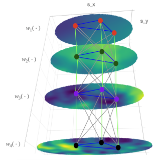
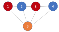
We visually illustrate stitching of univariate GPs to build a GGP $w(\cdot)$, satisfying (i)-(iii) above. Figure 1 (left) shows realizations of 4 univariate Matérn GPs $w_{i}(\cdot)$, $i=1,\ldots,4$, each with a different smoothness and spatial range. Figure 1 (right) shows a multivariate GGP constructed by stitching together the 4 processes using a path-graph as $\mathcal{G}_{\mathcal{V}}$ with $E_{\mathcal{V}}=\{(i,i+1):i=1,2,3\}$. We begin our construction on $\mathcal{L}$, a finite but otherwise arbitrary set of locations in $\mathcal{D}$ (the 3 locations in Figure 1 (right)). We first ensure that $w(\mathcal{L})=(w_{1}(\mathcal{L}),\ldots,w_{q}(\mathcal{L}))^{\mathrm{\scriptscriptstyle T}}$satisfies conditions (i)-(iii) when the domain is restricted to $\mathcal{L}$. This is achieved by stitching together the variables at the 3 locations in $\mathcal{L}$ such that there is a thread (edge) between two variable-location pairs if and only if there is an edge between the two corresponding variables in $\mathcal{V}$. We then stitch each of the remaining surfaces independently so that they have the same distribution as the univariate surfaces from the left panel and conforms to the graph at the process-level. This resembles stitching the four surfaces together at the locations $\mathcal{L}$, while exactly preserving each univariate surface. The graph edges serve as the threads holding the surfaces together.

Turning to the formal development, we first create $w(\mathcal{L})$—the realisation of our target process $w(\cdot)$ on $\mathcal{L}$ that satisfies properties (i)-(iii) on $\mathcal{L}$. Combining the three requirements, we model $w(\mathcal{L})\sim N(0,M(\mathcal{L},\mathcal{L}))$, seeking a p.d. matrix $M(\mathcal{L},\mathcal{L})$ such that

1. $M_{ii}(\mathcal{L},\mathcal{L})=C_{ii}(\mathcal{L},\mathcal{L})$ for all $i=1,\ldots,q$, to satisfy (i);

2. $(M(\mathcal{L},\mathcal{L})^{-1})_{ij}=0$ for all $(i,j)\notin E_{\mathcal{V}}$ to satisfy (ii).

3. $M_{ij}(\mathcal{L},\mathcal{L})=C_{ij}(\mathcal{L},\mathcal{L})$ for all $(i,j)\in E_{\mathcal{V}}$, to satisfy (iii).

Existence of such a matrix $M(\mathcal{L},\mathcal{L})$ is a covariance selection problem (Dempster, 1972).

Lemma 2.3 (Covariance selection (Dempster, 1972)).

Given a graph $\mathcal{G}=(\mathcal{S},E)$ and any p.d. matrix $F=(F_{rs})$ indexed by $\mathcal{S}\times\mathcal{S}$, there exists a unique p.d. matrix $\widetilde{F}=(\widetilde{F}_{rs})$ such that $\widetilde{F}_{rs}=F_{rs}$ for $r=s$ or for $(r,s)\in E_{\mathcal{S}}$, and $(\widetilde{F}^{-1})_{rs}=0$ for $(r,s)\notin E_{\mathcal{S}}$.

To ensure that the covariances and cross-covariances are preserved over $\mathcal{L}$ for all $i$ and all $(i,j)\in E_{\mathcal{V}}$ and the conditional independence among elements of $w(\mathcal{L})$ are inherited from $\mathcal{G}_{\mathcal{V}}$, $w(\mathcal{L})$ needs to conform to a graph with edges between variable-location pairs as in Figure 1. Formally, let $\mathcal{G_{L}}=(\mathcal{L},E_{\mathcal{L}})$ be the complete graph on the set of locations $\mathcal{L}$. The variable-location graph from Figure 1 (right) is the strong product graph $\mathcal{G_{V}}\boxtimes\mathcal{G_{L}}$. Here, $\mathcal{G}_{V}\boxtimes\mathcal{G}_{L}=(\mathcal{V}\times\mathcal{L},E_{\mathcal{V}\times\mathcal{L}})$ with $\mathcal{V}\times\mathcal{L}=\{(i,l):i\in\mathcal{V},\;l\in\mathcal{L}\}$ and $E_{\mathcal{V}\times\mathcal{L}}$ comprises edges between vertex-pairs $(i,l)$ and $(i^{\prime},l^{\prime})$ based upon the following strong-product adjacency rules: (i) $i=i^{\prime}$ and $(l,l^{\prime})\in E_{\mathcal{L}}$; or (ii) $l=l^{\prime}$ and $(i,i^{\prime})\in E_{\mathcal{V}}$; or (iii) $(i,i^{\prime})\in E_{\mathcal{V}}$ and $(l,l^{\prime})\in E_{\mathcal{L}}$.

Applying Lemma 2.3 with the vertex set $\mathcal{S}=\mathcal{V}\times\mathcal{L}$, positive definite matrix $F=C(\mathcal{L},\mathcal{L})$ and the graph $\mathcal{G}_{V}\boxtimes\mathcal{G}_{L}$, ensures the existence and uniqueness of a positive definite matrix $\widetilde{F}=M(\mathcal{L},\mathcal{L})$ satisfying conditions (a), (b) and (c) above. In practice, $M(\mathcal{L},\mathcal{L})$ can be obtained using an iterative proportional scaling (IPS) algorithm (Speed et al., 1986; Xu et al., 2011).

Note that Condition (b) only ensures conditional independence of the process restricted to $\mathcal{L}$. Process-level conditional independence over the entire domain $\mathcal{D}$ follows from the subsequent extension in (2) as proved in Theorem 2.5. Having built the finite-dimensional distribution of $w(\mathcal{L})$ from $\mathcal{G}_{\mathcal{V}}\boxtimes\mathcal{G}_{\mathcal{L}}$, we now suitably extend it to a well-defined multivariate GP $w(\cdot)$ over the domain ${\mathcal{D}}$, which conforms to the conditional dependencies implied by $\mathcal{G}_{\mathcal{V}}$. We leverage the following well-known decomposition of a GP $w_{i}(\cdot)$ as sum of a finite rank predictive process $w_{i}^{*}(\cdot)=E(w_{i}(\cdot)\,|\,w_{i}(\mathcal{L}))$ and an independent residual process $z_{i}(\cdot)$ (Banerjee et al., 2008; Finley et al., 2009):

$$w_{i}(s)=w_{i}^{*}(s)+z_{i}(s)=C_{ii}(s,\mathcal{L})C_{ii}(\mathcal{L},\mathcal{L})^{-1}w_{i}(\mathcal{L})+z_{i}(s)\quad\mbox{ for all}\quad s\in\mathcal{D}\setminus\mathcal{L}\;,$$ (2)

where each $z_{i}(\cdot)$ is a zero-centred Gaussian Process, independent of $w(\mathcal{L})$, with the valid covariance function $C_{ii\,|\,\mathcal{L}}(s,s^{\prime})=C_{ii}(s,s^{\prime})-C_{ii}(s,\mathcal{L})C^{-1}_{ii}(\mathcal{L},\mathcal{L})C_{ii}(\mathcal{L},s^{\prime})$.

The first part of stitching ensures that $w(\mathcal{L})$ conforms to $\mathcal{G}_{\mathcal{V}}$ when restricted to $\mathcal{L}$. The next result establishes process-level conditional independence for the stitched predictive process.

Lemma 2.4.

The predictive process $w^{*}(\cdot)=(w^{*}_{1}(\cdot),\ldots,w_{q}^{*}(\cdot))^{{\mathrm{\scriptscriptstyle T}}}$ is a GGP$(\mathcal{G}_{\mathcal{V}})$ on $\mathcal{D}$.

We now extend the finite-rank GGP $w^{*}(\cdot)$ to a full-rank GGP $w(\cdot)$ over the entire domain $\mathcal{D}$ through (2). We construct $z_{i}(\cdot)\sim GP(0,C_{ii|\mathcal{L}})$ such that $z_{i}(\cdot)\perp z_{j}(\cdot)$ for all $i\neq j$, and $z_{i}(\cdot)\perp w(\mathcal{L})$ for all $i$. Independence among $z_{i}(\mathcal{L})$ and $w(\mathcal{L})$ and the marginal covariance of $z_{i}(\mathcal{L})$ in (2) ensures that each $w_{i}(\cdot)$ on $\mathcal{D}$ is exactly $GP(0,C_{ii})$. However, independence among the $z_{i}(\cdot)$’s is a neat choice ensuring that the conditional independence relations in $\mathcal{G}_{\mathcal{V}}$ is extended from the finite set $\mathcal{L}$ to the spatial process over $\mathcal{D}$. We prove this formally in Theorem 2.5.

Theorem 2.5.

Given a cross-covariance function $C$ and an inter-variable graph $\mathcal{G}_{\mathcal{V}}$, stitching creates a valid multivariate GGP $w(\cdot)$ with a valid (p.d.) cross-covariance function $M$ such that:

1. $w_{i}(\cdot)\sim GP(0,C_{ii})$ , i.e., $M_{ii}(s,s^{\prime})=C_{ii}(s,s^{\prime})$ for all $s,s^{\prime}\in\mathcal{D}$ and for each $i=1,\ldots,q$,

2. $w(\cdot)$ is a GGP$(\mathcal{G}_{\mathcal{V}})$ on $\mathcal{D}$,

3. if $(i,j)\in E_{\mathcal{V}}$, then $M_{ij}(s,s^{\prime})=C_{ij}(s,s^{\prime})$ for all $s,s^{\prime}\in\mathcal{L}$.

Stitching produces a multivariate GP $w(\cdot)$ that exactly satisfies the first two conditions sought in Section 2.1. Regarding Condition (iii), we point out some differences between the GGP ensured by Theorem 2.2 and the one produced by stitching. For pairs of variables $(i,j)\in E_{\mathcal{V}}$, the cross-covariance for the former is exactly the same as the given cross-covariance $C_{ij}$ on the entire domain $\mathcal{D}$, whereas for the latter $M_{ij}(s,s^{\prime})=C_{ij}(s,s^{\prime})$ for locations in $\mathcal{L}$. For a pair $s,s^{\prime}\notin\mathcal{L}$ and $i\neq j$ it is straightforward to verify that

$$M_{ij}(s,s^{\prime})=C_{ii}(s,\mathcal{L})C_{ii}(\mathcal{L},\mathcal{L})^{-1}M(\mathcal{L},\mathcal{L})_{ij}C_{jj}(\mathcal{L},\mathcal{L})^{-1}C_{jj}(\mathcal{L},s^{\prime})\;.$$ (3)

Stitching, thus, produces a computationally feasible GGP with desired full-rank marginal covariance and process-level conditional independence at the expense of allowing a fixed rank cross-covariance. Choosing $\mathcal{L}$ to be reasonably dense (well-spaced) in $\mathcal{D}$, we have $M_{ij}(s,s^{\prime})\approx C_{ij}(s,s^{\prime})$ for $(i,j)\in E_{\mathcal{V}}$, $s,s^{\prime}\in\mathcal{D}\setminus\mathcal{L}$. Hence, condition (iii) is satisfied exactly on $\mathcal{L}$ and approximately on $\mathcal{D}\setminus\mathcal{L}$ for the stitched GP.

3 Highly multivariate Graphical Matérn Gaussian processes

3.1 Incompatibility of multivariate Matérn with graphical models

Theorems 2.2 and 2.5 establish, respectively, the existence of and the construction of a marginal-preserving GGP given any valid cross-covariance $C$ and any inter-variable graph $\mathcal{G}_{\mathcal{V}}$. We are particularly interested in developing a novel class of multivariate graphical Matérn GPs that are GGP$(\mathcal{G}_{\mathcal{V}})$ such that each univariate process is a Matérn GP. This is appealing for inference as we retain the ability to interpret the parameters for each univariate spatial process. We achieve this using stitching, which is necessary as we argue below that no non-trivial parametrisation of the existing multivariate Matérn GP yields a GGP.

The isotropic multivariate Matérn cross-covariance function on a $d$-dimensional domain is $C_{ij}(s,s^{\prime})=\sigma_{ij}H_{ij}(\|s-s^{\prime}\|)$, where $H_{ij}(\cdot)=H(\cdot\,|\,\nu_{ij},\phi_{ij})$, $H$ being the Matérn correlation function (Apanasovich et al., 2012). If $\theta_{ij}=\{\sigma_{ij},\nu_{ij},\phi_{ij}\}$, then for a multivariate Matérn GP the $i$th individual variable is a Matérn GP with parameters $\theta_{ii}$. This is attractive because it endows each univariate process with its own variance $\sigma_{ii}$, smoothness $\nu_{ii}$, and spatial decay $\phi_{ii}$. Another nice property is that under this model, $\Sigma=(\sigma_{ij})=\mbox{Cov}(w(s))$ is the covariance matrix for $w(s)$ within each location $s$. The cross-correlation parameters $\nu_{ij}$ and $\phi_{ij}$ for $i\neq j$, are generally hard to interpret, especially since $\nu_{ij}$ does not correspond to the smoothness of any surface. Recent work by Kleiber (2017) on the concept of coherence has facilitated some interpretation of these parameters. The parsimonious multivariate Matérn model of Gneiting et al. (2010) emerges from this general specification as a special case with $\nu_{ij}=(\nu_{ii}+\nu_{jj})/2$ and $\phi_{ij}=\phi$.

To ensure a valid multivariate Matérn cross-covariance function, it is sufficient to constrain the intra-site covariance matrix $\Sigma=(\sigma_{ij})$ to be of the form (Theorem 1, Apanasovich et al., 2012)

$$\begin{array}[]{cc}\sigma_{ij}=&b_{ij}\frac{\Gamma(\frac{1}{2}(\nu_{ii}+\nu_{jj}+d))\Gamma(\nu_{ij})}{\phi_{ij}^{2\Delta_{A}+\nu_{ii}+\nu_{jj}}\Gamma(\nu_{ij}+\frac{d}{2})}\mbox{ where }\Delta_{A}\geq 0,\mbox{ and }B=(b_{ij})>0,\mbox{ i.e., is p.d.}\end{array}$$ (4)

This is equivalent to $\Sigma$ being constrained as $\Sigma=(B\odot(\gamma_{ij}))$, where $\gamma_{ij}$ are constants collecting the terms in (4) involving only $\nu_{ij}$’s and $\phi_{ij}$’s, and $\odot$ denotes the Hadamard (element-wise) product. Similarly, the spectral density matrix takes the form $F(\omega)=(B\odot(g_{ij}(\omega)))$, where $g_{ij}(\omega)$ are functions involving the parameters $\phi_{ij}$ and $\nu_{ij}$. The matrix $B=(b_{ij})$’s are the $O(q^{2})$ parameters (free of $\phi_{ij}$’s or $\nu_{ij}$’s) that are constrained to ensure $B$ is positive-definite. Process-level conditional independences introduce zeros in the inverse of the spectral density matrix for stationary processes (see, e.g., Theorem 2.4 in Dahlhaus (2000)). This implies that, for any parametrisation of the multivariate Matérn GP to be a GGP, we need $(F(\omega)^{-1})_{ij}=0$ for every $(i,j)\notin E_{\mathcal{V}}$ and almost all $\omega$. From the Hadamard product $F(\omega)=(B\odot(g_{ij}(\omega)))$, it is clear that zeros in $B^{-1}$ or $\Sigma^{-1}$ do not generally imply zeros in $F^{-1}(\omega)$ for the multivariate Matérn. An exception occurs when each component is posited to have the same smoothness $\nu$ and the same spatial decay parameter $\phi$, whence both $\Sigma$ and $F(\omega)$ become proportional to $B$. In this case, zeros in $B^{-1}$ (specified according to $\mathcal{G}_{\mathcal{V}}$) will correspond to zeros in $\Sigma^{-1}$ and $F^{-1}(\omega)$ yielding a GGP with respect to $\mathcal{G}_{\mathcal{V}}$. However, assuming $\nu_{ij}=\nu$ and $\phi_{ij}=\phi$ for all $(i,j)$ implies that the univariate GPs have the same smoothness and rate of spatial decay, which is restrictive. Beyond this separable model, there is, to the best of our knowledge, no known parameter choice for the multivariate Matérn GPs that will allow it to be a GGP$(\mathcal{G}_{\mathcal{V}})$.

3.2 Computational considerations for stitching

Stitching univariate processes corresponding to a valid multivariate Matérn cross-covariance $C$ and a graph $\mathcal{G}_{\mathcal{V}}$ yields a multivariate graphical Matérn GP such that (i) the univariate processes are exactly Matérn; (ii) the multivariate process conforms to process-level conditional independence relations as specified by $\mathcal{G}_{\mathcal{V}}$; and (iii) the cross-covariances for pairs of variables in $\mathcal{G}_{\mathcal{V}}$ are exactly or approximately Matérn (see Eq. 3). For each $i=1,2,\ldots,q$ let $D_{i}$ be the set of $n_{i}$ locations where the $i$-th variable has been observed. The joint probability density of $w_{i}(D_{i})$ and $w(\mathcal{L})$ is specified by $w(\mathcal{L})\sim N(0,M(\mathcal{L},\mathcal{L}))$ and

$$\begin{array}[]{c}w_{i}(D_{i})\,|\,w(\mathcal{L})\stackrel{{\scriptstyle ind}}{{\sim}}N(C_{ii}(D_{i},\mathcal{L})C_{ii}(\mathcal{L},\mathcal{L})^{-1}w_{i}(\mathcal{L}),C_{ii\,|\,\mathcal{L}}(D_{i},D_{i}))\;\mbox{ for }i=1,\ldots,q\;.\end{array}$$ (5)

The covariance matrix for $\{w_{i}(D_{i}):\,i=1,\ldots,q\}\,|\,w(\mathcal{L})$ is block-diagonal with variable-specific blocks and is cheap to compute if all of the $n_{i}$’s are small. If some $n_{i}$’s are large, we can use one of the several variants of scalable GPs for very large number of locations (Heaton et al., 2019). For example, a nearest neighbour GP (NNGP, Datta et al., 2016) yields a sparse approximation of $C_{ii\,|\,\mathcal{L}}(D_{i},D_{i})$ with linear complexity, but the joint distribution still preserves the conditional independence implied by $\mathcal{G}_{\mathcal{V}}$.

When $q$ is large, note that $\{w_{i}(D_{i}):\,i=1,\ldots,q\}\,|\,w(\mathcal{L})$ in (5) has $q$ conditionally independent factors and is easy to compute in parallel. However, the likelihood for $w(\mathcal{L})\sim N(0,M(\mathcal{L},\mathcal{L}))$ presents the bottleneck for this highly multivariate case. In particular, there are two challenges for large $q$. As discussed earlier, the multivariate Matérn $C$ required for stitching needs to constrain $B=(b_{ij})$ to be p.d. on an $O(q^{2})$-dimensional parameter space. Searching in such a high-dimensional space is difficult for large $q$ and verifying positive definiteness of $B$ incurs an additional cost of $O(q^{3})$ flops. Second, evaluating $w(\mathcal{L})\sim N(0,M(\mathcal{L},\mathcal{L}))$ involves matrix operations for the $nq\times nq$ matrix $M(\mathcal{L},\mathcal{L})$. While the precision matrix, $M(\mathcal{L},\mathcal{L})^{-1}$, is sparse because of $\mathcal{G}_{V}$, its determinant is usually not available in closed form and the calculation can become prohibitive even for small $n$.

3.3 Decomposable variable graphs

To facilitate scalability in highly multivariate settings, we consider decomposable inter-variable graphs. For $\mathcal{G}_{\mathcal{V}}=(\mathcal{V},E)$, and a triplet $(A,B,O)$ of disjoint subsets $\mathcal{V}$, $O$ is said to separate $A$ from $B$ if every path from $A$ to $B$ passes through $O$. If $\mathcal{V}=A\cup B\cup O$, and $O$ induces a complete subgraph of $\mathcal{V}$, then $(A,B,O)$ is said to decompose $\mathcal{G}_{\mathcal{V}}$. The graph $\mathcal{G}_{\mathcal{V}}$ is said to be decomposable if it is complete or if there exists a proper decomposition $(A,B,O)$ into decomposable subgraphs $\mathcal{G}_{A\cup O}$ and $\mathcal{G}_{B\cup O}$. Several naturally occurring dependence structures like low-rank dependence or autoregressive dependence correspond to decomposable graphs (see Section 4). More generally, if a graph is non-decomposable, it can be embedded in a larger decomposable graph. Hence, assuming decomposability is conspicuous in graphical models (see, e.g., Dobra et al., 2003; Wang & West, 2009) since fitting Bayesian graphical models is cumbersome for non-decomposable graphs (Roverato, 2002; Atay-Kayis & Massam, 2005).

Table 1: Properties of any $q$-dimensional multivariate Matérn GP of Gneiting et al. (2010) or Apanasovich et al. (2012) and a multivariate graphical Matérn GP stitched using a decomposable graph $\mathcal{G}_{V}$ with largest clique size $q^{*}$ (typically $\ll q$), length of perfect ordering $p$, and maximal number of cliques $p^{*}$ sharing a common vertex.

Model attributes	Multivariate Matérn	Multivariate Graphical Matérn
Number of parameters	$O(q^{2})$	$O(|E_{\mathcal{V}}|+q)$
Parameter constraints	$O(q^{3})$	$O(p^{*}(q^{*3}))$ (worst case)
Storage	$O(n^{2}q^{2})$	$O(pn^{2}q^{*2})$ (worst case)
Time complexity	$O(n^{3}q^{3})$	$O(pn^{3}q^{*3})$ (worst case)
Conditionally independent processes	No	Yes
Univariate components are Matérn GPs	Yes	Yes

For stitching of Matérn GPs using decomposable graphs we can significantly reduce the dimension of the parameter space, storage and computational burden. Let $K_{1},\cdots,K_{p}$ be a sequence of subsets of the vertex set $\mathcal{V}$ for an undirected graph $\mathcal{G}_{\mathcal{V}}$. Let, $F_{m}=K_{1}\cup\cdots\cup K_{m}$ and $S_{m}=F_{m-1}\cap K_{m}$. The sequence $\{K_{m}\}$ is said to be perfect if (i) for every $l>1$, there is an $m<l$ such that $S_{l}\subset K_{m}$; and (ii) the separator sets $S_{m}$ are complete for all $m$. If $\mathcal{G}_{V}$ is decomposable, then it has a perfect clique sequence (Lauritzen, 1996) and the joint density of $w(\mathcal{L})$ can be factorized as follows.

Corollary 3.1.

If $\mathcal{G_{V}}$ has a perfect clique sequence $\{K_{1},K_{2},\cdots,K_{p}\}$ with separators $\{S_{2},\ldots,S_{m}\}$, then the GGP likelihood on $\mathcal{L}$ can be decomposed as

$$f_{M}(w(\mathcal{L}))=\frac{\Pi_{m=1}^{p}f_{C}(w_{K_{m}}(\mathcal{L}))}{\Pi_{m=2}^{p}f_{C}(w_{S_{m}}(\mathcal{L}))}\;,$$ (6)

where $f_{A}$ denotes the density of a GP over $\mathcal{L}$ with covariance function $A$ for $A\in\{M,C\}$.

Corollary 3.1 helps us manage the dimension and constraints of the parameter space and the computational complexity of stitching. For an arbitrary $\mathcal{G}_{V}$, the parameter space for the stitching covariance function $M$ is the same as the parameter space $\{\theta_{ij}|1<i,j\leq q\}$ for the original covariance function $C$. For a decomposable $\mathcal{G}_{V}$, the likelihood (6) and, in turn, the stitched GGP is only specified by the parameters $\{\theta_{ij}\,|\,(i=j)\mbox{ or }(i,j)\in E_{\mathcal{V}}\}$. Therefore, the dimension of the parameter space reduces from $O(q^{2})$ to $O(|E_{\mathcal{V}}|+q)$ , where $|E_{\mathcal{V}}|$ is the number of edges on $\mathcal{G}_{\mathcal{V}}$, which is small for sparse graphs. When using a multivariate Matérn cross-covariance $C$ for stitching, the parameter space for $B$ in the stitched graphical Matérn is the intersection of the parameter spaces of the low-dimensional clique-specific multivariate Matérn covariance functions $C_{K_{1}},\ldots,C_{K_{p}}$. Hence, the parameter space becomes $\{b_{ij}|(i=j)\mbox{ or }(i,j)\in E_{\mathcal{V}}\}$ and needs to satisfy the constraint that $B_{K_{l}}=(b_{ij})_{i,j\in K_{l}}$ is p.d. for all $l=1,\ldots,p$. This reduces the computational complexity of parameter constraints from $O(q^{3})$ to at most $O(p^{*}q^{*3})$, where $q^{*}$ is the largest clique size and $p^{*}$ is the maximum number of cliques sharing a common vertex. The precision matrix of $w(\mathcal{L})$ satisfies (Lemma 5.5, Lauritzen, 1996)

$$M(\mathcal{L},\mathcal{L})^{-1}=\sum_{m=1}^{p}[{C}_{[K_{m}\boxtimes\mathcal{G_{L}}]}^{-1}]^{\mathcal{V}\times\mathcal{L}}-\sum_{m=2}^{p}[{C}_{[S_{m}\boxtimes\mathcal{G_{L}}]}^{-1}]^{\mathcal{V}\times\mathcal{L}}\;,$$ (7)

where, for any symmetric matrix $A=(a_{ij})$ with rows and columns indexed by ${\cal U}\subset\mathcal{V}\times\mathcal{L}$, $A^{\mathcal{V}\times\mathcal{L}}$ denotes a $|{\mathcal{V}\times\mathcal{L}}|\times|{\mathcal{V}\times\mathcal{L}}|$ matrix such that $(A^{\mathcal{V}\times\mathcal{L}})_{ij}=a_{ij}$ if $(i,j)\in{\cal U}$, and $(A^{\mathcal{V}\times\mathcal{L}})_{ij}=0$ elsewhere. From (6) and (7) we see that the stitching likelihood evaluation avoids the large matrix $M(\mathcal{L},\mathcal{L})$ and all matrix operations are limited to the sub-matrices of $M(\mathcal{L},\mathcal{L})$ corresponding to the cliques $K_{m}\boxtimes\mathcal{G_{L}}$ and separators $S_{m}\boxtimes\mathcal{G_{L}}$. The entire process requires at most $O(pn^{3}q^{*3})$ flops and $O(pn^{2}q^{*2})$ storage, where $p$ is the length of the perfect ordering. Table 1 summarizes these gains from stitching with decomposable graphs.

The computational efficiency of stitching is clear from the above. In addition, the following result shows that the GGP likelihood from stitching yields unbiased estimating equations for all parameters included in the GGP (all marginal and cross-covariance parameters for any pairs of variables included in $\mathcal{G}_{\mathcal{V}}$) under model misspecification when the data is generated from a multivariate Matérn GP, but is modelled as a graphical Matérn GP with a decomposable $\mathcal{G}_{\mathcal{V}}$.

Proposition 3.2.

Let $w(\cdot)\sim GP(0,C(\cdot,\cdot))$, where $C$ is a valid $q\times q$ multivariate Matérn cross-covariance function with parameters $\{\theta_{ij}:1\leq i,j\leq q\}$, and $f_{M}(w(\mathcal{L}))$ denotes the multivariate graphical Matérn GP likelihood (6) from stitching using a decomposable graph $\mathcal{G}_{\mathcal{V}}$. Then $E(\partial\log f_{M}(w(\mathcal{L}))/\partial\theta_{ij})=0$ for any $i=j$ or $(i,j)\in E_{\mathcal{V}}$.

3.4 Chromatic Gibbs sampler

With a valid process specification for $w(\cdot)$, we cast (1) into a hierarchical model over the $n$ observed locations in ${\mathcal{S}}$ and sample from the posterior distribution derived from

$$p(\beta,\tau,\theta)\times N(w(\mathcal{S})\,|\,0,C_{\theta}(\mathcal{S},\mathcal{S}))\times\prod_{j=1}^{n}N(y(s_{j})\,|\,X(s_{j})\beta+w(s_{j}),D_{\tau})\;,$$ (8)

where $X(s_{j})=\mbox{diag}(x_{1}(s_{j})^{{\mathrm{\scriptscriptstyle T}}},x_{2}(s_{j})^{{\mathrm{\scriptscriptstyle T}}},\ldots,x_{q}(s_{j})^{{\mathrm{\scriptscriptstyle T}}})$ is $q\times(\sum_{i=1}^{q}p_{i})$, $\beta=(\beta_{1}^{{\mathrm{\scriptscriptstyle T}}},\beta_{2}^{{\mathrm{\scriptscriptstyle T}}}\ldots,\beta_{q}^{{\mathrm{\scriptscriptstyle T}}})^{{\mathrm{\scriptscriptstyle T}}}$, $w(\mathcal{S})=(w(s_{1})^{{\mathrm{\scriptscriptstyle T}}},w(s_{2})^{{\mathrm{\scriptscriptstyle T}}}\ldots,w(s_{n})^{{\mathrm{\scriptscriptstyle T}}})^{{\mathrm{\scriptscriptstyle T}}}$, $D_{\tau}=\mbox{diag}(\tau^{2}_{1},\tau^{2}_{2},\ldots,\tau^{2}_{q})$, $\theta$ is the set of parameters in the cross-covariance function and $p(\beta,\tau,\theta)$ is a prior distribution on model parameters. Besides the computational benefits described in Table 1, stitched GGP models are also amenable to parallel computing. In a Bayesian implementation of a stitched GGP model (described in Section S2.1 of the Supplement), we can exploit the graph $\mathcal{G}_{V}$ and deploy a chromatic Gibbs sampler (Gonzalez et al., 2011) to simultaneously update batches of random variables in parallel. Let $\eta_{i}$ be the vector grouping variable-specific parameters (regression coefficients, spatial parameters, noise variance and latent spatial random effects). Under a graph colouring of $\mathcal{G}_{V}$, $\eta_{i}$ and $\eta_{i^{\prime}}$ can be updated simultaneously if $i$ and $i^{\prime}$ share the same colour, as illustrated in Figure 2 (left).

Figure 2: Chromatic sampling for GGP with a gem graph between $5$ variables: Left: Gem graph and colouring used for chromatic sampling of the variable-specific parameters. Right: Colouring of the corresponding edge graph $\mathcal{G}_{E}(\mathcal{G}_{V})$ used for chromatic sampling of the cross-covariance parameters $b_{ij}$’s.

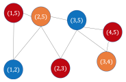
This brings down the number of sequential steps in sampling of the $\eta_{i}$’s from $q$ to the chromatic number $\chi(\mathcal{G}_{V})$. We can also employ a chromatic sampling scheme for the $b_{ij}$’s, but using a different graph. We exploit the fact that the parameters $b_{ij}$ and $b_{i^{\prime}j^{\prime}}$ belongs to the same factor in (6) for a pair of edges $(i,j)$ and $(i^{\prime},j^{\prime})$ in $E_{\mathcal{V}}$ if and only if the variables $i,j,i^{\prime},j^{\prime}$ belongs to the same clique. Thus, if $\mathcal{G}_{E}(\mathcal{G}_{V})=(E_{\mathcal{V}},E^{*})$ denotes this graph on the set of edges $E_{\mathcal{V}}$, i.e., there is an edge $((i,j),(i^{\prime},j^{\prime}))$ in this new graph $\mathcal{G}_{E}(\mathcal{G}_{V})$ if $\{i,i^{\prime},j,j^{\prime}\}$ are in some clique $K$ of $\mathcal{G}_{V}$, then we can batch the updates of $b_{ij}$’s based on the colouring of the graph $\mathcal{G}_{E}(\mathcal{G}_{V})$ (Figure 2 (right)). The number of such sequential batch updates will be the chromatic number $\chi(\mathcal{G}_{E}(\mathcal{G}_{V}))$, a potentially drastic reduction from $|E_{\mathcal{V}}|$ sequential updates for $b_{ij}$.

4 Extensions

4.1 Factor models

The construction of GGP and its implementation described in Sections 2 and 3 assumes a known graphical model. Here, we describe different avenues for choosing or estimating the graph and offer extensions of GGP to model different spatial and spatiotemporal structures.

In many multivariate spatial models, the inter-variable graphical model arises naturally and is decomposable. A large subset of multivariate spatial models are process-level factor models (emerge from more general linear models of coregionalization (LMC)), where each of the $q$ observed univariate processes are a weighted sum of $r\leq q$ latent univariate factor processes with the weights being component-specific (Schmidt & Gelfand, 2003; Gelfand et al., 2004; Wackernagel, 2013). In general, a linear model of coregionalization can be expressed as

$$w_{i}(s)=\sum_{j=1}^{r}a_{ij}(s)f_{j}(s)+\xi_{i}(s)\;,$$ (9)

where each $f_{j}(\cdot)$ is a latent factor process such that $f(\cdot)=(f_{1}(\cdot),\ldots,f_{r}(\cdot))^{\mathrm{\scriptscriptstyle T}}$ is a multivariate GP, $a_{ij}(\cdot)$’s are component-specific weight functions and $\xi(\cdot)$ are independent processes representing the idiosyncratic spatial variation in $w_{i}(\cdot)$ not explained by the latent factors. If $q$ is large, choosing $r\ll q$ in (9) also facilitates dimension reduction (Lopes et al., 2008; Ren & Banerjee, 2013; Taylor-Rodriguez et al., 2019; Zhang & Banerjee, 2021). We next show that any linear model of coregionalization can be formulated as a GGP with a decomposable graph on the elements of $w(\cdot)$ and $f(\cdot)$.

Proposition 4.1.

Consider the linear model of coregionalization (9) where $f(\cdot)$ is an $r\times 1$ multivariate GP with a complete graph between component processes, and $\xi_{i}(\cdot)$’s are independent univariate GPs. Then $(w_{1},w_{2},\ldots,w_{q},f_{1},\ldots,f_{r})^{\mathrm{\scriptscriptstyle T}}$ is a GGP on vertices $\{1,\dots,q+r\}$ and a decomposable graph $\{(i,j)|i\in 1,\ldots,(q+r),j\in(q+1),\ldots,(q+r),j\neq i\}$.

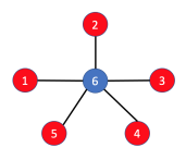
Proposition 4.1 dictates that the assumption of multivariate dependence induced through factor processes can be translated into a decomposable graph between the observed and factor processes. Hence, GGPs can be used as a richer alternative to the linear model of coregionalization. While the linear model of coregionalization enforces all processes $w_{i}(\cdot)$ to have the smoothness of the roughest $f_{j}(\cdot)$ (Genton & Kleiber, 2015), the GGP enables us to model and interpret the spatial smoothness of each component process (e.g., with the graphical Matérn GP). The complete graph between the $r$ component processes of $f(\cdot)$ can be assumed without loss of generality as even for a sparse graph between latent factors (e.g., when the factors are independent processes), they will generally be conditionally dependent given the observed processes $w(\cdot)$, thereby yielding the same joint graph. Due to $r\ll q$, this joint graph of observed and latent processes will still be sparse even after considering all possible edges between latent processes. Figure 3 illustrates two examples of the decomposable graphs arising from linear model of coregionalization.

(a) $2$ observed (red) and $2$ latent (blue) processes

(b) $5$ observed (red) and $1$ latent (blue) processes

Figure 3: Decomposable graphs for (a) a full rank and (b) a low-rank linear model of coregionalization.

An alternative approach to linear models of coregionalization builds multivariate spatial processes by sequentially modelling a set of univariate GPs conditional from some ordering of the $q$ variables (Cressie & Zammit-Mangion, 2016). A sparse partial ordering can facilitate dimension reduction for large $q$. This approach does not attempt to preserve marginals or introduce process-level conditional independence. However, a partial ordering yields a directed acyclic graph (DAG), which, when moralised, produces a decomposable undirected graph that can be used in our stitched GGPs.

4.2 Non-separable spatial time-series modelling

GGPs are natural candidates for non-separable (in space-time), non-stationary (in time) modelling of univariate or multivariate spatial time-series. Consider a univariate spatial time-series modelled as a GP $\{w(s,t)\}$ for $s\in\mathcal{D}$ evolving over a discrete set of time points $t\in\mathcal{T}=\{1,2,\ldots,T\}$. We envision this as a $T\times 1$ GP $w(s)=(w_{1}(s),\ldots,w_{T}(s))^{{\mathrm{\scriptscriptstyle T}}}$, where $w_{t}(s)=w(s,t)$. Temporal evolution of processes is often encapsulated using a directed acyclic graph (DAG), which, when moralized, produces an undirected graph $\mathcal{G}_{\mathcal{T}}$ over $\mathcal{T}$. We can then recast the spatial time-series model as a $T\times 1$ GGP with respect to $\mathcal{G}_{\mathcal{T}}$. A multivariate Matérn used for stitching will produce a GGP with each $w_{t}(\cdot)$ being a Matérn GP with parameters $\theta_{tt}$. Time-specific process variances and spatial parameters enrich the model without imposing stationarity of the spatial process over time and space-time separability (Gneiting, 2002).

Any autoregressive (AR) structure over time corresponds to a decomposable moralized graph $\mathcal{G}_{\mathcal{T}}$. For example, the $AR(1)$ model corresponds to a path graph with edges $\{(t,t+1)\,|\,t=1,\ldots,T-1\}$, $q^{*}=2$ and $p^{*}=2$. An $AR(2)$ is specified by the DAG $t-2\to t$ and $t-1\to t$ for all $t\in\{3,\ldots,T\}$ (Figure S8a in the Supplement), which, when moralized, yields the sparse decomposable graph $\mathcal{G}_{\mathcal{T}}$ (with $q^{*}=3$) in Figure S8b of the Supplement. Hence, Corollary 3.1 accrues computational gains for GGP models for autoregressive spatial time-series. An added benefit of using the GGP is that the auto-regression parameters need not be universal, but can be time-specific, thus relaxing another restrictive stationarity condition.

GGP allows the marginal variances and autocorrelations of the processes to vary over time and be estimated in an unstructured manner. However, more structured temporal models for stochastic volatility can be easily accommodated by a GGP if forecasting the process at a future time-point is of interest. This can be achieved by adding a model for the time-specific variances like the log-AR(1) model as considered in Jacquier et al. (1993). Bayesian estimation of these model parameters has been discussed in Jacquier et al. (2002) and can be seamlessly incorporated into our Bayesian framework for estimation of GGP parameters.

Multivariate spatial time-series can also be modelled using GGP. We envision $q$ variables recorded at $T$ time-points resulting in $qT$ variables. We now specify $\mathcal{G}_{\mathcal{V}\times\mathcal{T}}$ on the variable-time set. Common specifications for multivariate time-series like graphical vector autoregressive (VAR) structures (Dahlhaus & Eichler, 2003) will yield decomposable $\mathcal{G}_{\mathcal{V}\times\mathcal{T}}$. For example, consider the non-separable graphical-VAR of order 1 with $q=2$ and specified by the DAG $(1,t-1)\to(1,t)$, $(1,t-1)\to(2,t)$, and $(2,t-1)\to(2,t)$ (Figure S8c of the Supplement). This yields the decomposable $\mathcal{G}_{\mathcal{V}\times\mathcal{T}}$ in Figure S8d of the Supplement, also with $q^{*}=3$.

4.3 Graph estimation

Sections 4.1 and 4.2 present settings where the decomposable graph for a GGP arises naturally. For gridded spatial data, one can use a spatial graphical lasso to estimate the graph from the sparse inverse spectral density matrix (Jung et al., 2015), and plug-in the estimated graph in subsequent estimation of GGP likelihood parameters. For irregularly located spatial data, we now extend our framework in (8) to infer about the graphical model itself along with the GGP parameters by adapting an MCMC sampler for decomposable graphs (Green & Thomas, 2013).

The junction graph $G$ of a decomposable $\mathcal{G}_{\mathcal{V}}$ is a complete graph with the cliques of $\mathcal{G}_{\mathcal{V}}$ as its nodes. Every edge in the junction graph is represented as a link, which is the intersection of the two cliques, and can be empty. A spanning tree of a graph is a subgraph comprising all the vertices of the original graph and is a tree (acyclic graph). Suppose a spanning tree $J$ of the junction graph of $G$ satisfies the following property: for any two cliques $C$ and $D$ of the graph, every node in the unique path between $C$ and $D$ in the tree contains $C\cap D$. Then $J$ is called the junction tree for the graph $\mathcal{G}_{\mathcal{V}}$ (see Figure 2 of Thomas & Green, 2009, for an illustration). A junction tree exists for $\mathcal{G}_{\mathcal{V}}$ if and only if $\mathcal{G}_{\mathcal{V}}$ is decomposable. Also, a decomposable graph can have many junction trees but each junction tree represents a unique decomposable graph. This allows us to transform a prior on decomposable graphs to a prior on the junction trees. If $\mu(\mathcal{G}_{\mathcal{V}}(J))$ is the number of junction trees for the decomposable graph $\mathcal{G}_{\mathcal{V}}$ corresponding to $J$, then a prior $\pi$ on decomposable graphs gives rise to a prior $\tilde{\pi}$ on the junction trees as $\tilde{\pi}(J)={\pi(\mathcal{G}_{\mathcal{V}}(J))}/{\mu(\mathcal{G}_{\mathcal{V}}(J))}$. In our application, we assume $\pi$ to be uniform over all decomposable graphs with a pre-specified maximum clique size, i.e., $\tilde{\pi}(J)\propto{1}/{\mu(\mathcal{G}_{\mathcal{V}}(J))}$.

With junction trees as a representative state variable for the graph, the jumps are governed by constrained addition or deletion of single/multiple edges so that the resulting tree is also a junction tree for some decomposable graph. Each graph corresponds to a different GGP model using a specific subset of the cross-covariance parameters. To embed sampling this graph within the Gibbs sampler in Section S2.1, jumps between graphs need to be coupled with introduction or deletion of cross-covariance parameters depending on addition or deletion of edges. We use the reversible jump MCMC (rjMCMC) algorithm of Barker & Link (2013) to carry out the sampling of the graph and cross-covariance parameters and lay out the details in Section S2.3.

4.4 Asymmetric covariance functions

Our examples of stitching have primarily involved the isotropic (symmetric) multivariate Matérn cross-covariances. Symmetry implies $C_{ij}(s,s^{\prime})=C_{ij}(s^{\prime},s)$ for all $i,j,s,s^{\prime}$ and is not a necessary condition for validity of a cross-covariance function. An asymmetric cross-covariance function (Apanasovich & Genton, 2010; Li & Zhang, 2011) $C^{a}$ can be specified in-terms of a symmetric cross-covariance $C$ as $C^{a}_{ij}(s,s^{\prime})=C^{a}_{ij}(s-s^{\prime})=C_{ij}(s-s^{\prime}+(a_{i}-a_{j}))$, where $a_{i}$, $i=1,\ldots,q$ are distinct variable specific parameters. Stitching works with any valid cross-covariance function, and if $C^{a}$ is used for stitching, then the resulting graphical cross-covariance $M^{a}$ will also be asymmetric, satisfying $M^{a}_{ij}(s,s^{\prime})=C^{a}_{ij}(s,s^{\prime})$ for all $(i,j)\in E_{\mathcal{V}}$, and $s,s^{\prime}\in\mathcal{L}$.

4.5 Response model

We outline a Gibbs sampler in Section S2.1 of the Supplement for the multivariate spatial linear model in (1), where the latent $q\times 1$ process $w(s)$ is modelled as a GGP. If $|\mathcal{L}|=n$, then the algorithm needs to sample $\sim O(nq)$ latent spatial random effects $w(\mathcal{L})$ at each iteration.

A popular method for estimating spatial process parameters in (1) is to integrate out the spatial random effects $w(\mathcal{L})$ and directly use the marginalized (or collapsed) likelihood for the response process $y(\cdot)=(y_{1}(\cdot),\ldots,y_{q}(\cdot))^{{\mathrm{\scriptscriptstyle T}}}$, which is also a multivariate GP. However, $w(\cdot)$ modelled as a GGP does not ensure that the marginalized $y(\cdot)$ will be a GGP. We demonstrate this in Figure 4(a) with a path graph $\mathcal{G}_{\mathcal{V}}$ between $3$ latent processes $w_{1}(\cdot)$, $w_{2}(\cdot)$ and $w_{3}(\cdot)$. The response processes $y_{i}(\cdot)=w_{i}(\cdot)+\epsilon_{i}(\cdot)$ have complete graphs. This is because $\mbox{Cov}(y)=\mbox{Cov}(w)+\mbox{Cov}(\epsilon)$, and the zeros in $\mbox{Cov}(w)^{-1}$ do not correspond to zeros in $\mbox{Cov}(y)^{-1}$. Hence, modelling the latent spatial process as a GGP and subsequent marginalization is inconvenient because the marginalized likelihood for $y$ will not factorize like (6).

(a) GGP on the latent process.

(b) GGP on the response process.

Figure 4: Comparison of induced graphs for $3$ processes (obeying a path graph) from marginalized model and latent model. Blue edges indicate the dependencies modelled and red edges denote the marginal dependencies induced from the model construction.

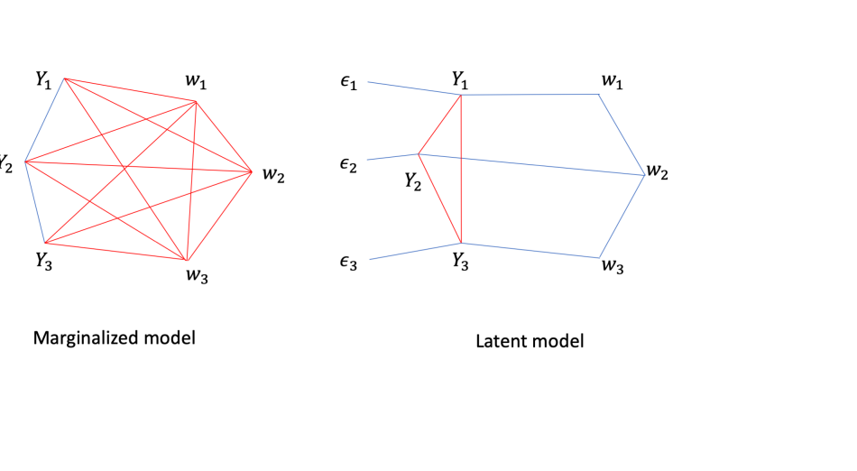
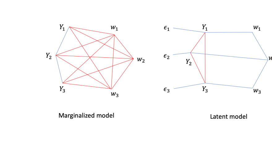
Instead, we can directly create a GGP for the response process by stitching the marginal cross-covariance function $\mbox{Cov}(y(s),y(s+h))=C(h)+D(h)$ using $\mathcal{G}_{\mathcal{V}}$, where $D(h)=\mbox{diag}(\tau^{2}_{1},\ldots,\tau^{2}_{q})I(h=0)$ is the diagonal white-noise covariance function. With a Matérn cross-covariance $C$, the resulting GGP model for $y(\cdot)$ endows each univariate GP $y_{i}(\cdot)$ with mean $x_{i}(\cdot)^{{\mathrm{\scriptscriptstyle T}}}\beta_{i}$ and retaining the marginal covariance function $C_{ii}(h)+\tau_{i}^{2}I(h=0)$ (i.e., Matérn plus a nugget). The cross-covariance between $y_{i}(\cdot)$ and $y_{j}(\cdot)$ is also Matérn for $(i,j)\in E_{\mathcal{V}}$ and locations in $\mathcal{L}$. For $(i,j)\notin\mathcal{G}_{V}$, the response processes $y_{i}(\cdot)$ and $y_{j}(\cdot)$ will be conditionally independent. We outline the Gibbs sampler for this response GGP in Section S2.2 of the Supplement.

The response model drastically reduces the dimensionality of the sampler from $O(nq+|E_{\mathcal{V}}|)$ for the latent model to $O(q+|E_{\mathcal{V}}|)$. What we gain in terms of convergence of the chain is traded off in interpretation of the latent process. As we see in Figure 4(b), using a graphical model on the response process leads to a complete graph among the latent process. If, however, conditional independence on the latent processes is not absolutely necessary, then the marginalized GGP model is a pragmatic alternative for modelling highly multivariate spatial data.

5 Simulations

5.1 Known graph

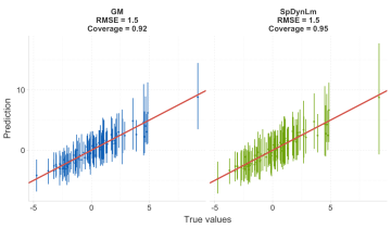
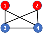
We conducted multiple simulation experiments to compare three models: (a) PM: Parsimonious Multivariate Matérn of Gneiting et al. (2010); (b) MM: Multivariate Matérn of Apanasovich et al. (2012) with $\nu_{ij}=\nu_{ii}=\nu_{jj}=\frac{1}{2}$, and $\Delta_{A}=0$ and $\phi^{2}_{ij}=(\phi^{2}_{ii}+\phi^{2}_{jj})/2$; and (c) GM: Graphical Matérn (GGP on the latent process, stitched using multivariate Matérn model (b)).

Table 2: Different simulation scenarios considered for the comparison between methods.

Set	$q$	Graph $\mathcal{G}_{\mathcal{V}}$	$B$	Nugget	Locations	Data model	Fitted models
1A	5	Gem (Figure 2(a))	Random	No	Same location for all variables	GM	GM, MM, PM
1B	5	Gem (Figure 2(a))	Random	No	Same location for all variables	MM	GM, MM, PM
2A	15	Path	$b_{i-1,i}=\rho_{i}$	Yes	Partial overlap in locations for variables	GM	GM, PM
2B	15	Path	$b_{i-1,i}=\rho_{i}$	Yes	Partial overlap in locations for variables	MM	GM, PM
3A	100	Path	$b_{i-1,i}=\rho_{i}$	Yes	Partial overlap in locations for variables	GM	GM
3B	100	Path	$b_{i-1,i}=\rho_{i}$	Yes	Partial overlap in locations for variables	MM	GM

We consider the 6 settings in Table 2. In Sets 1A, 2A, and 3A, we generate data from GM. Set 1A has $q=5$ and uses a gem graph (Figure 2 (a)). For Set 2A, we considered $q=15$ outcomes and used a path graph, while Set 3A considers the highly multivariate case with $q=100$ outcomes and a path graph. Sets 1B–3B are same as Sets 1A–3A, respectively, except that we generate data from MM. Thus the scenarios 1A–3A correspond to correctly specified settings for the GGP, while scenarios 1B–3B serve as misspecified examples where data is generated from MM. For all scenarios, we generated data on $n=250$ locations uniformly chosen over a grid. We simulated 1 covariate $x_{j}(s_{i})$ for each variable $j$, generated independently from a $N(0,4)$ distribution and the true regression coefficients $\beta_{j}$ from Unif(-2,2) for $j=1,2,\ldots,q$.

(a) Set 1B

(b) Set 2B

(c) Set 3B

(d) Set 1B

Figure 5: Performance of graphical Matérn under misspecification: (a), (b) and (c): Estimates of the cross-covariance parameters $\sigma_{ij}\phi_{ij}=\Gamma(1/2)b_{ij}$, $(i,j)\in E_{\mathcal{V}}$ for the sets 1B, 2B and 3B respectively. The pink lines in Figures (a) and (b) indicate true parameter values. (d): Median RMSPE for GM, MM, PM and Independent GP model for Set 1B.

The $\phi_{ii}$ and $\sigma_{ii}$ were equispaced numbers in $(1,5)$, while the $b_{ij}$’s where chosen as in Table 2. For all of the candidate models, each component of the $q$-variate process is a Matérn GP. Following the recommendation outlined in Apanasovich et al. (2012), the marginal parameters $\theta_{ii}$ for the univariate Matérn processes were estimated apriori using only the data for the $i$-th variable. The BRISC R-package (Saha & Datta, 2018) was used for estimation.

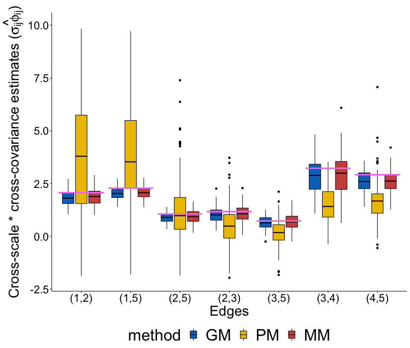
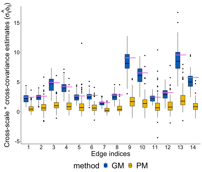
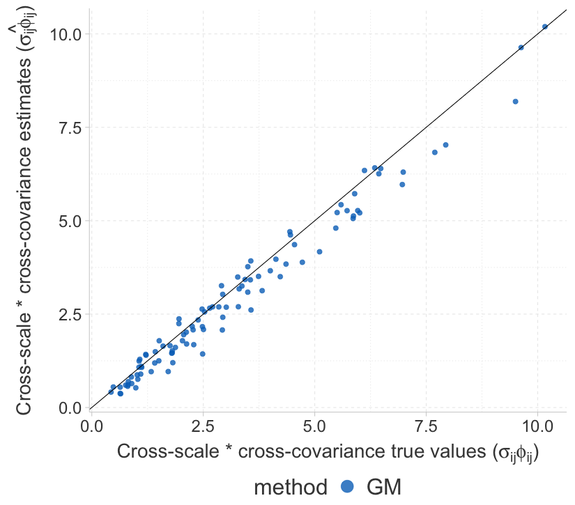
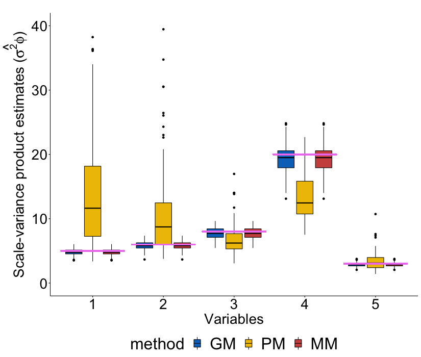
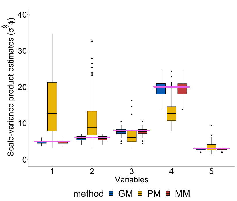
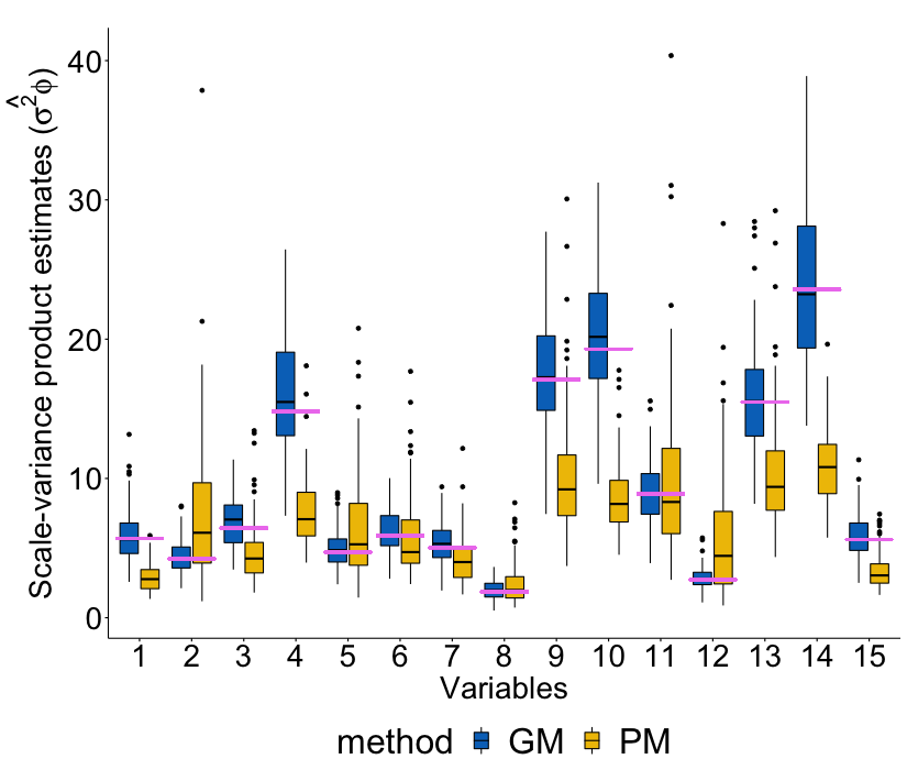
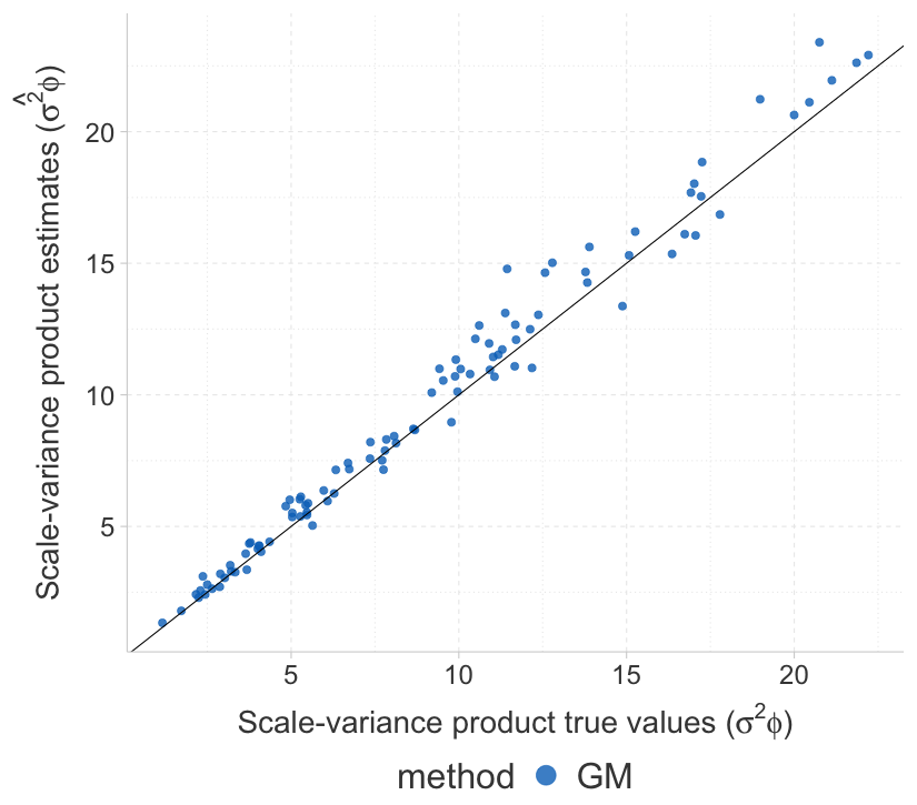
To compare estimation performance, we primarily focus on the cross-covariance parameters $b_{ij}$, $(i,j)\in E_{\mathcal{V}}$, as they specify the cross-covariances in stitching. Specifically, we compare the estimates of $\sigma_{ij}\phi_{ij}=\Gamma(1/2)b_{ij}$, which are the $b_{ij}$’s rescaled to be at the same scale as the marginal microergodic parameters $\sigma_{ii}\phi_{ii}$. Model evaluations under the correctly specified settings of 1A–3A are provided in Supplementary Figure S9, which reveals that the GGP accurately estimates cross-covariance parameters for all the edges in the graph for all 3 scenarios. Figures 5 (a), (b), and (c), evaluate the estimates of GM for the misspecified settings 1B, 2B and 3B, respectively. For Set 1B we see that MM, and GM produce reasonable estimates of the true cross-covariance parameters included, whereas the estimates from PM are biased and more variable. For Set 2B the estimates of PM are once again biased, while GM is more accurate.

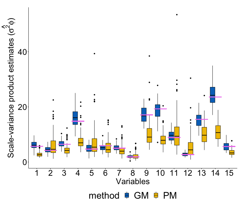
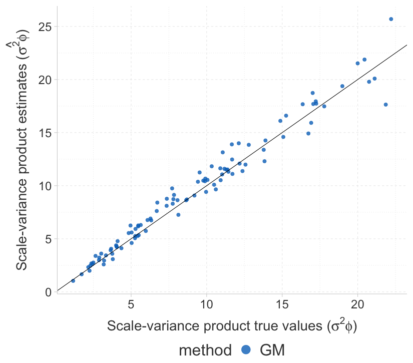
For the highly multivariate settings in Sets 3A and 3B, neither PM nor MM can be implemented because $B$ involves $4,950$ parameters and likelihood evaluation requires inverting a $25,000\times 25,000$ matrix in each iteration. Hence, we only compare the estimates from GGP to the truth. Figure S9c shows that the GGP performs well in the highly multivariate setting with misspecification (3B) with GM once again accurately estimating all the $b_{ij}$’s for $(i,j)\in E_{\mathcal{V}}$. These simulations under misspecification confirm the accuracy of GGP in estimating $b_{ij}$ for the MM for pairs $(i,j)$ included in the graph and aligns with the conclusion from Proposition 3.2.

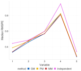
We also evaluate the impact of misspecification on the predictive performance. Figure 5d plots the root mean square predictive error (RMSPE) based on hold-out data for Set 1B. In addition to the models listed in Table 2 we also consider a model where each component GP is an independent Matérn GP serving as a reference for the impact of not modelling dependence. We find GM performs competitively with MM (the correctly specified model) yielding nearly identical RMSPEs for all the 5 variables. PM yields higher RMSPE for variables $1$ and $3$, while the independent model is, unsurprisingly, the least accurate. Additional analyses and discussions are in the Supplementary materials (Section S3). These include comparison of marginal parameter estimates (Section S3.1), impact of excluding edges on estimation of cross-correlation functions (Section S3.2), comparison of GGP with dynamic linear models for spatial time series (Section S3.4), comparison of GGP with linear model of coregionalization (Section S3.3), and comparison among different variants of the GM model (Section S3.5).

5.2 Unknown graph

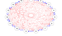
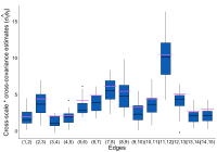
We also evaluated our model when the graph is unknown and is sampled using the reversible jump MCMC sampler described in Section 4.3. We consider simulation scenarios in Sets 1A and 2A from Table 2, where the true multivariate process is a graphical Matérn. We assess the accuracy of inferring about the graphical model and the estimates of the cross-covariance parameters. We visualise the estimated edge probabilities for Set 2A in Figure 6(a). The blue edges correspond to the true edges, while red ones correspond to false edges. The width of the edges are proportional to the posterior probability of selecting that edge. We see that most of the false edges have narrow width indicating their low selection probability. We report the top 20 probable edges estimated by our model in Table S3 of the Supplement and observe that our approach ranks all the $14$ true edges higher than any of the false edges in terms of marginal probability. Figure 6(b) shows that the cross-covariance parameters corresponding to true edges are also estimated correctly. The results for Set 1A are similar and presented in Figure S10.

(a) Posterior edge selection probabilities for Set 2A.

(b) Cross-covariance parameter estimates for Set 2A while estimating the unknown graph

Figure 6: Performance of GGP with unknown graph for Set 2A: (a): Marginal edge probabilities estimated from the reversible jump MCMC sampler. Blue edges denote the true edges and red denotes the non-existent edges. Edges are weighted proportional to the estimated posterior selection probabilities. (b) GM estimates of cross-correlation parameters ($b_{ij}$) corresponding to true edges when the graph is unknown, with horizontal pink lines indicating the true values.

6 Spatial modelling of PM_2.5 time-series

We demonstrate an application of GGP for non-stationary (in time) and non-separable (in space-time) modelling of spatial time-series (Section 4.2). We model daily levels of PM_2.5 measured at monitoring stations across 11 states of the north-eastern US and Washington DC for a three month period from February, 01, 2020, until April, 30th, 2020. The data is publicly available from the website of the United States Environmental Protection Agency (EPA).

We selected $n=99$ stations with at least two months of measured data for both $2020$ and $2019$. Meteorological variables such as temperature, barometric pressure, wind-speed and relative humidity are known to affect PM_2.5 levels. Since all of the pollutant monitoring stations do not measure all these covariates, we collected the data from NCEP North American Regional Reanalysis (NARR) database, and merged it with the available weather data from EPA to impute daily values of these covariates at pollutant monitoring locations using multilevel B-spline smoothing. Also to adjust for baseline PM_2.5 levels, for each station and day in 2020, we included a $7$-day moving average of the PM_2.5 data for that station centered around the same day of $2019$ as a baseline covariate We adjust for weekly periodicity of PM_2.5 levels by subtracting day-of-the-week specific means from raw PM_2.5 values. Following Section 4.2, we view the spatial time-series at $n=99$ locations and $T=89$ days as a highly multivariate ($89$-dimensional) spatial data set. Neither the parsimonious Matérn nor the multivariate Matérn were implementable as they involve $89^{2}/2\approx 4000$ cross-covariance parameters and $9000\times 9000$ matrix computations ($99\times 89\approx 9000$) in each iteration.

(a) Prediction performance for fortnightly analysis

(b) Prediction performance for full analysis

(c) Log-variance estimates for the full analysis

(d) Estimates of time-specific cross-correlations

(e) Average residual surfaces

Figure 7: PM_2.5 analysis: (a) Daily RMSPE for the 6 fortnightly analyses, (b) Daily RMSPE for the full analyses, (c) Estimates of the time-specific process variances, (d) Estimates and credible intervals of the cross-correlation parameters $r_{t,t-1}$ (corresponding to the cross-covariances $b_{t,t-1}$), (e) Estimates of the residual spatial processes from GM (after adjusting for covariates and baseline) for first two weeks of February and last two weeks of April.

We used a graphical Matérn GP with an $AR(1)$ graph based upon exploratory analysis that revealed autocorrelation among pollutant processes on consecutive days after adjusting for covariates. The marginal parameters for day $t$ were $\sigma_{tt},\phi_{tt}$ and $\tau^{2}_{t}$. The autoregressive cross-covariance between days $t-1$ and $t$ is $b_{t-1,t}$. Hence, GGP offers the flexibility to model non-separability across space and time, time-varying marginal spatial parameters and autoregressive coefficients.

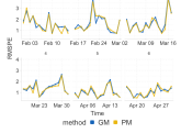
We first present a subgroup analysis breaking $89$ days worth of data into $6$ fortnights. Data for each fortnight is only $14$ or $15$ dimensional and, hence, we are able to analyse each chunk separately using the parsimonious Matérn (PM). Figure 7a presents hold-out RMSPE and reveals that GM and PM produce very similar predictive performance when analysing each fortnight of data separately. We analyse the full dataset using the GGP model (GM) as other multivariate Matérn GPs like PM are precluded by the highly multivariate setting. The GGP model involves only $88$ cross-covariance parameters. Since the largest clique size in an AR(1) graph is $2$, the largest matrix we deal with for the data at $99$ stations is only $198\times 198$. We also consider spatiotemporal models that can model non-stationary and non-separable relationships in the data. Gneiting (2002) developed general classes of non-separable spatiotemporal models. However, these models assume a stationary temporal process. More importantly, likelihood for this model will involve a dense $9000\times 9000$ matrix over the set of all space-time pairs and is generally impracticable for modelling long spatial time-series.

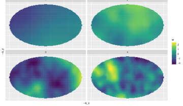
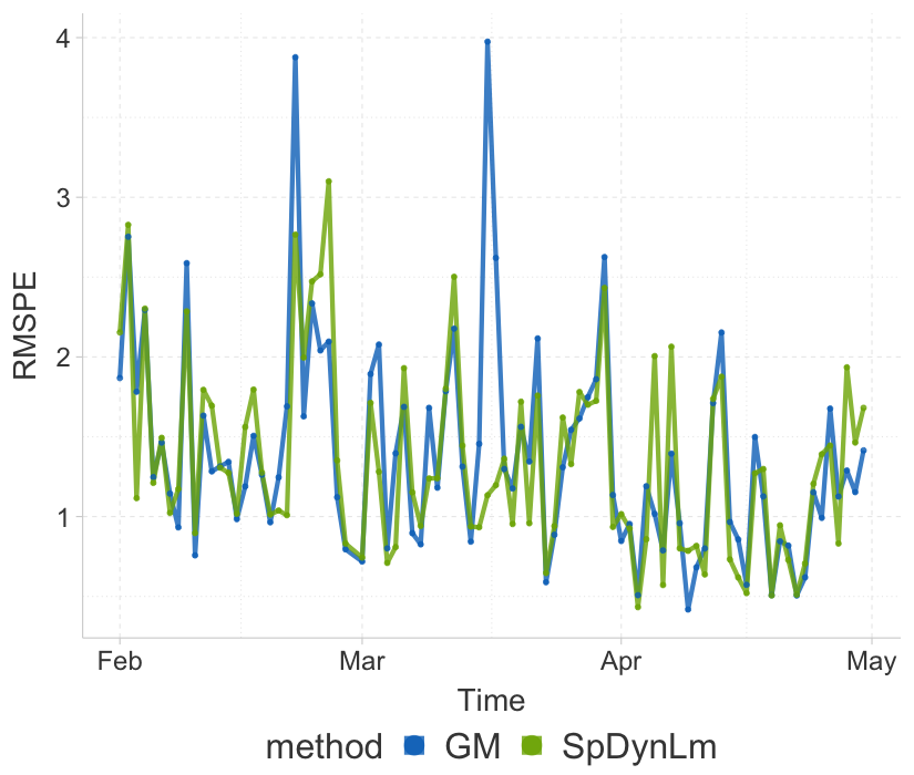
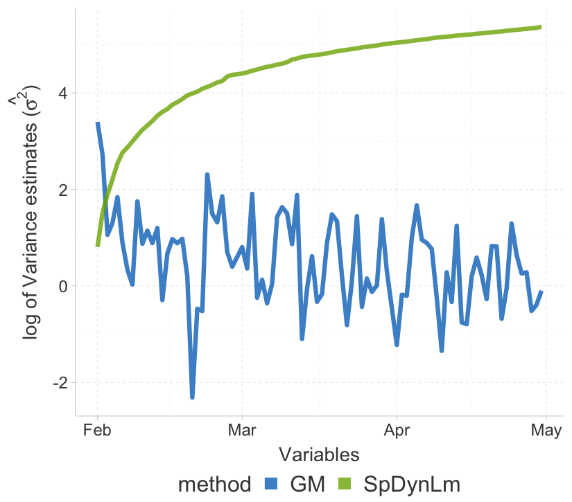
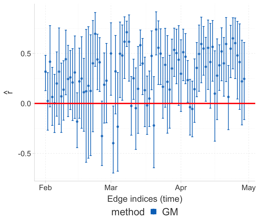
For the full analysis, we compare GGP with a spatial dynamic linear model (Stroud et al., 2001; Gelfand et al., 2005) that, like GGP, can parsimoniously model the temporal evolution using an $AR(1)$ structure and allows both non-separability and time-specific parameters. We use the SpDynLm function currently offered in the spBayes package (see Section S3.4 of the Supplement for details). Predictive performance is similar for both models with respect to both point predictions (Figure 7b) and interval predictions (Figure S11). Figure 7c plots variance estimates (in the log-scale) over time of the latent processes. The implementation in spBayes uses the customary random-walk prior to model for the AR(1) evolution. This enforces these marginal variances to be monotonically increasing resulting in unrealistically large variance estimates for later time-points. The estimates from GGP show substantial variation across time with generally a decreasing trend going from February to April. The estimates and credible intervals for the auto-correlation parameters $r_{t,t-1}$ (normalized $b_{t,t-1}$) from GGP are presented in Figure 7d. There is large variation in these estimates across time with many spikes indicating high positive autocorrelation. Quantitatively, $95\%$ Bayesian credible intervals for $40$ out of the $88$ ($45\%$) $r_{t,t-1}$ estimates from GM exclude $0$ providing strong evidence in favour of non-stationary auto-correlation across time. SpDynLm does not have an analogous auto-correlation parameter, and, hence, cannot be compared in this regard.

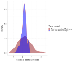
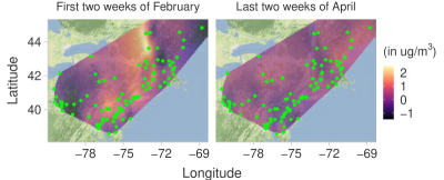
The estimated average residual spatial surface, $y_{\mathcal{P}}(s)=(1/|\mathcal{P}|)\sum_{t\in\mathcal{P}}(y_{t}(s)-x_{t}(s)^{{\mathrm{\scriptscriptstyle T}}}\hat{\beta}_{t})$, is depicted in Figure 7e for two choices of the time-period $\mathcal{P}$–the first two weeks of February, 2020 (left), and the last two weeks of April, 2020 (right). These two periods represent the beginning and end of the time period for our study and also correspond to before and during lock-downs imposed in the north-eastern US due to COVID-19. We observe a slight decrease in the magnitude of the residual process from February (median across locations: $0.181$) to April (median across locations: $0.164$) (Figure S12) suggesting a decrease in the PM_2.5 levels during this period even after accounting for the meteorological covariates and the previous year’s level as a baseline. The residuals for April also showed much lesser variability compared to that in February, suggesting a decrease in the latent process variance over time. This agrees with the estimates of $\sigma_{tt}$ from GGP (Figure 7c) and contradicts the strongly increasing variance estimates from SpDynLm (see Section S3.4 for a broader discussion).

7 Discussion

This high-dimensional problem we address here accounts for large number of variables and is distinctly different from the burgeoning literature on high-dimensional problems referring to the massive number of spatial locations. A future direction will be to simultaneously address the problem of big $n$ and big $q$ by extending stitching to nearest neighbor location graphs with sparse variable graphs. Relaxing the assumption of linear covariate effects $x_{i}^{\mathrm{\scriptscriptstyle T}}\beta_{i}$ in (1) can also be pursued as discussed recently by Saha et al. (2021). A multivariate analogue of this would benefit from the sparse precision matrices available from stitching (7). Finally, the idea of stitching can be transported to the discrete spatial (areal) setting to create multivariate analogs of the interpretable Directed Acyclic Graph Auto-regressive (DAGAR) models (Datta et al., 2019), where stitching would preserve the univariate marginals being exactly DAGAR distributions.

7.1 ACKNOWLEDGEMENT

A. Datta gratefully acknowledges financial support from the National Science Foundation Division of Mathematical Sciences grant DMS-1915803. S. Banerjee gratefully acknowledges support from NSF grants, DMS-1916349 and DMS-2113778, and from NIH grants NIEHS-R01ES030210 and NIEHS-R01ES027027. This work was completed through a fellowship supported by a Joint Graduate Training Program between the Department of Biostatistics at the Johns Hopkins Bloomberg School of Public Health and the Intramural Research Program of the National Institute of Mental Health. The authors are grateful to the Editor, Associate Editor and anonymous reviewers for their feedback which helped to improve the manuscript.

Supplementary Materials for “Graphical Gaussian Process Models for Highly Multivariate Spatial Data”

S1 Proofs

Proof S1.1 (of Theorem 2.2).

Part (a). For the original GP, $F(\omega)=\{f_{ij}(\omega)\}$ is a valid spectral density matrix. Therefore, following Cramer’s Theorem (Cramér, 1940; Parra & Tobar, 2017), $F(\omega)$ is positive definite (p.d.) for (almost) every frequency $\omega$. Using Lemma 2.3 we derive a unique $\widetilde{F}(\omega)=(\widetilde{f}_{ij}(\omega))$, which is also positive definite and satisfies $\widetilde{F}(\omega)_{ij}=F(\omega)_{ij}=f_{ij}(\omega)$ for $i=j$ or $(i,j)\in E_{\mathcal{V}}$, and $\widetilde{F}(\omega)^{-1}_{ij}=0$ for $(i,j)\notin E_{\mathcal{V}}$. The square-integrability assumption of $f_{ii}(\omega)$ is sufficient to ensure that $\int|\widetilde{f}_{ij}(\omega)|d\omega<\infty$ using the Cauchy-Schwarz inequality. Thus, we have a spectral density matrix $\widetilde{F}(\omega)$, which is positive definite for (almost) all $\omega$, $\widetilde{f}_{ii}(\omega)=f_{ii}(\omega)>0$ for all $i$, $\omega$, and $\int|\widetilde{f}_{ij}(\omega)|d\omega<\infty$ for all $i,j$. By Cramer’s theorem, there exists a GP $w(\cdot)$ with spectral density matrix $\widetilde{F}(\omega)$ and some cross-covariance function $M$. As by construction $\widetilde{f}_{ij}(\omega)=f_{ij}(\omega)$ for $i=j$ or $(i,j)\in E_{\mathcal{V}}$, we have $M_{ij}=C_{ij}$ for $i=j$ or $(i,j)\in E_{\mathcal{V}}$. Since $\widetilde{F}^{-1}(\omega)_{ij}=0$ for $(i,j)\notin E_{\mathcal{V}}$ and almost all $\omega$, using the result of Dahlhaus (2000), $w(s)$ has process-level conditional independence on $\mathcal{D}$ as specified by $\mathcal{G}_{\mathcal{V}}$, completing the proof.

Part (b). Let $K(\omega)\in\mathcal{F}$. By definition, $K(\omega)$ corresponds to the spectral density matrix of a GGP with respect to $\mathcal{G}_{\mathcal{V}}$. By Theorem 2.4 in Dahlhaus (2000)), $(K(\omega)^{-1})_{ij}=0$ for all $(i,j)\notin E_{\mathcal{V}}$ and almost all $\omega$. Let $S(K)$ denote the collection of $\omega$ for which this happens. From the construction of $\tilde{F}$ in part (a), for each $\omega\in S(K)$ we thus have $(K(\omega)^{-1})_{ij}=(\tilde{F}(\omega)^{-1})_{ij}=0$ for all $(i,j)\notin E_{\mathcal{V}}$ and $\tilde{F}(\omega)_{ij}=F(\omega)_{ij}$ for all $(i,j)\in E_{\mathcal{V}}$. Using property (c) of Dempster (1972), we have

$$\operatorname{tr}(K(w)^{-1}F(\omega))+\log\det(K(\omega))\geq\operatorname{tr}(\tilde{F}(w)^{-1}F(\omega))+\log\det(\tilde{F}(\omega))\;\forall\;\omega\in S(K).$$

As $S(K)^{c}$ has measure zero, integrating this over $S(K)$ produces the inequality in part (b).

Proof S1.2 (of Lemma 2.4).

Consider any $(i,j)\notin E_{\mathcal{V}}$, and $s,s^{\prime}\in\mathcal{D}$. Let $B=\mathcal{V}\setminus\{i,j\}$ and $\mathcal{A}$ denote the $\sigma$-algebra $\sigma(\{w^{*}_{k}(s)\,|\,s\in\mathcal{D},k\in B\})$. As $w^{*}_{k}(s)=C_{kk}(s,\mathcal{L})C_{kk}(\mathcal{L},\mathcal{L})^{-1}w_{k}(\mathcal{L})$ is a deterministic function of $w_{k}(\mathcal{L})$ for all $k,s$, we have $\mathcal{A}\subseteq\sigma(w_{B}(\mathcal{L}))$. On the other hand, as $w_{k}(s)=w_{k}^{*}(s)$ for all $s\in\mathcal{L}$ (predictive process agrees with the original process at the knot locations) we have $\sigma(w_{B}(\mathcal{L}))\subseteq\sigma(\mathcal{A})$. Hence, $\sigma(w_{B}(\mathcal{L}))=\sigma(\mathcal{A})$. Now we have

$$Cov(w_{i}^{*}(s),w_{j}^{*}(s^{\prime})\,|\,\mathcal{A})=Cov(w_{i}^{*}(s),w_{j}^{*}(s^{\prime})\,|\,\sigma(w_{B}(\mathcal{L}))$$ (S1)

$$\quad=C_{ii}(s,\mathcal{L})C_{ii}(\mathcal{L},\mathcal{L})^{-1}Cov(w_{i}(\mathcal{L}),w_{j}(\mathcal{L})\,|\,\sigma(w_{B}(\mathcal{L}))C_{jj}(\mathcal{L},\mathcal{L})^{-1}C_{jj}(\mathcal{L},s^{\prime})$$ (S2)

$$\qquad=0.$$ (S3)

The last equality follows directly from the construction of stitching for $w(\mathcal{L})$.

Proof S1.3 (of Theorem 2.5).

For two arbitrary locations $s_{1},s_{2}\in\mathcal{D}$, we can calculate the covariance function from our construction as follows:

$$\begin{array}[]{cl}M_{ij}(s_{1},s_{2})&=Cov\left(C_{ii}(s_{1},\mathcal{L})C_{ii}(\mathcal{L},\mathcal{L})^{-1}w_{i}(\mathcal{L})+z_{i}(s_{1}),\right.\\ &\qquad\left.C_{jj}(s_{2},\mathcal{L})C_{jj}(\mathcal{L},\mathcal{L})^{-1}w_{j}(\mathcal{L})+z_{j}(s_{2})\right)\\ &=C_{ii}(s_{1},\mathcal{L})C_{ii}(\mathcal{L},\mathcal{L})^{-1}Cov(w_{i}(\mathcal{L}),w_{j}(\mathcal{L}))C_{jj}(\mathcal{L},\mathcal{L})^{-1}C_{jj}(\mathcal{L},s_{2}))+\\ &\qquad\mathbb{I}(i=j)C_{ii\,|\,\mathcal{L}}(s_{1},s_{2})\\ &=\mathbb{I}(i=j)[C_{ii}(s_{1},\mathcal{L})C_{ii}(\mathcal{L},\mathcal{L})^{-1}C_{ii}(\mathcal{L},s_{2}))+C_{ii\,|\,\mathcal{L}}(s_{1},s_{2})]+\\ &\qquad\mathbb{I}(i\neq j)C_{ii}({\bm{s}}_{1},\mathcal{L})C_{ii}(\mathcal{L},\mathcal{L})^{-1}M_{ij}(\mathcal{L},\mathcal{L})C_{jj}(\mathcal{L},\mathcal{L})^{-1}C_{jj}(\mathcal{L},s_{2})\\ &=\mathbb{I}(i=j)C_{ii}(s_{1},s_{2})+\\ &\qquad\mathbb{I}(i\neq j)C_{ii}(s_{1},\mathcal{L})C_{ii}(\mathcal{L},\mathcal{L})^{-1}M_{ij}(\mathcal{L},\mathcal{L})C_{jj}(\mathcal{L},\mathcal{L})^{-1}C_{jj}(\mathcal{L},s_{2}))\end{array}$$ (S4)

The second equality follows from the independence of $z_{i}$ and $z_{j}$ for $i\neq j$, the third equality uses $M_{ii}(\mathcal{L}\mathcal{L})=C_{ii}(\mathcal{L},\mathcal{L})$ and the fourth uses the form of the conditional covariance function $C_{ii\,|\,\mathcal{L}}$ from (2). It is now immediate, that $w_{i}$ has the covariance function $C_{ii}$ on the entire domain $\mathcal{D}$, proving Part (a).

To prove part (b), without loss of generality we only consider $q=3$ processes $w_{1}(s),w_{2}(s),w_{3}(s)$ which is constructed via stitching, with the assumption that $(1,3)\notin E_{\mathcal{V}}$. First, we will show that, for any two locations $s_{1},s_{2}\in\mathcal{D}$, $w_{1}(s_{1})$ is conditionally independent of $w_{3}(s_{2})$ given $w_{2}(\mathcal{L})$, which we denote as $w_{1}(s_{1})\mathchoice{\mathrel{\hbox to0.0pt{$\displaystyle\perp$\hss}\mkern 2.0mu{\displaystyle\perp}}}{\mathrel{\hbox to0.0pt{$\textstyle\perp$\hss}\mkern 2.0mu{\textstyle\perp}}}{\mathrel{\hbox to0.0pt{$\scriptstyle\perp$\hss}\mkern 2.0mu{\scriptstyle\perp}}}{\mathrel{\hbox to0.0pt{$\scriptscriptstyle\perp$\hss}\mkern 2.0mu{\scriptscriptstyle\perp}}}w_{3}(s_{2})\,|\,w_{2}(\mathcal{L})$.

As $(1,3)\notin E_{\mathcal{V}}$, the sets $\{1\times\mathcal{L}\}=\{(1,s)\,|\,s\in\mathcal{L}\}$ and $\{3\times\mathcal{L}\}$ are separated by $\{2\times\mathcal{L}\}$ in the graph $\mathcal{G}_{V}\boxtimes\mathcal{G}_{L}$. Hence, using the global Markov property of Gaussian graphical models, we have $w_{1}(\mathcal{L})\mathchoice{\mathrel{\hbox to0.0pt{$\displaystyle\perp$\hss}\mkern 2.0mu{\displaystyle\perp}}}{\mathrel{\hbox to0.0pt{$\textstyle\perp$\hss}\mkern 2.0mu{\textstyle\perp}}}{\mathrel{\hbox to0.0pt{$\scriptstyle\perp$\hss}\mkern 2.0mu{\scriptstyle\perp}}}{\mathrel{\hbox to0.0pt{$\scriptscriptstyle\perp$\hss}\mkern 2.0mu{\scriptscriptstyle\perp}}}w_{3}(\mathcal{L})\,|\,w_{2}(\mathcal{L})$.

For any $s_{1},s_{2}\in\mathcal{D}$ we have, similar to (S4),

$$\begin{array}[]{cl}Cov(w_{1}(s_{1})w_{3}(s_{2})\,|\,w_{2}(\mathcal{L}))\\ =C_{11}(s_{1},\mathcal{L})C_{11}(\mathcal{L},\mathcal{L})^{-1}Cov\left(w_{1}(\mathcal{L}),w_{3}(\mathcal{L})\,|\,w_{2}(\mathcal{L})\right)C_{33}(\mathcal{L},\mathcal{L})^{-1}C_{33}(\mathcal{L},s_{2})=0.\end{array}$$

Hence, $w_{1}(s_{1})\mathchoice{\mathrel{\hbox to0.0pt{$\displaystyle\perp$\hss}\mkern 2.0mu{\displaystyle\perp}}}{\mathrel{\hbox to0.0pt{$\textstyle\perp$\hss}\mkern 2.0mu{\textstyle\perp}}}{\mathrel{\hbox to0.0pt{$\scriptstyle\perp$\hss}\mkern 2.0mu{\scriptstyle\perp}}}{\mathrel{\hbox to0.0pt{$\scriptscriptstyle\perp$\hss}\mkern 2.0mu{\scriptscriptstyle\perp}}}w_{3}(s_{2})\,|\,w_{2}(\mathcal{L})$ for any $s_{1},s_{2}\in\mathcal{D}$. Now

$$\begin{array}[]{cl}Cov(w_{1}(s_{1}),\,w_{3}(s_{2})\,|\,\sigma\left(\{w_{2}(s)\,|\,s\in\mathcal{D}\}\right))\\ =Cov(w_{1}(s_{1}),\;w_{3}(s_{2})\,|\,\sigma\left(w_{2}(\mathcal{L}),\{z_{2}(s)\,|\,s\in\mathcal{D}\}\right))\\ =Cov(w_{1}(s_{1}),\;w_{3}(s_{2})\,|\,\sigma\left(w_{2}(\mathcal{L})\right))=0.\end{array}$$ (S5)

The second inequality follows due to the agreement of the two conditioning $\sigma$-algebras (similar to the argument in the proof of Lemma  2.4). The third inequality follows from the fact that for any three random variables $X,Y$ and $Z$ such that $X$ and $Y$ are independent of $Z$, $E(X|Y,Z)=E(X|Y)$. Equation (S5) establishes process level conditional independence for $w_{1}(\cdot)$ and $w_{3}(\cdot)$ given $w_{2}(\cdot)$, thereby proving part (b).

Finally, if $(i,j)\in E_{\mathcal{V}}$, and $(s_{1},s_{2})\in\mathcal{L}$, in (S4), we will have $M_{ij}(s_{1},s_{2})=C_{ij}(s_{1},s_{2})$ directly from the construction of $M(\mathcal{L},\mathcal{L})$. This proves part (c).

Proof S1.4 (of Corollary 3.1).

Recall from the construction of $M(\mathcal{L},\mathcal{L})$ that the Gaussian random vector $w(\mathcal{L})$ satisfies the graphical model $\cal{G}=\mathcal{G_{V}}\boxtimes\mathcal{G_{L}}$, where $\cal{G_{L}}$ is the complete graph between $n$ locations. The strong product graph $\mathcal{G}$ is decomposable and $K_{m}\boxtimes\mathcal{G_{L}};m=1,\cdots,p$ form a perfect sequence for $\mathcal{G}$ with $S_{m}\boxtimes\mathcal{G_{L}};m=2,\cdots,p$ being the separators. Thus, using results (3.17) and (5.44) from Lauritzen (1996), we are able to factorize $w(\mathcal{L})$ as (6).

Proof S1.5 (of Proposition 3.2).

Suppose, we observe a Multivariate Matérn process. Under the assumption of Graphical Gaussian Processes, the resulting maximum likelihood estimating equations for parameters $\theta_{ij}$ belonging to cliques or separators ($i=j$ or $(i,j)\in E_{\mathcal{V}}$) are given by -

$$\begin{split}&\frac{\partial\log(f_{M}(w(\mathcal{L}))}{\partial{\theta_{ij}}}=0\\ \implies&\frac{\partial}{\partial{\theta_{ij}}}\left(\sum_{K}\log(f_{C}(w_{K}(\mathcal{L}))-\sum_{S}\log(f_{C}(w_{S}(\mathcal{L}))\right)=0\\ \implies&\frac{\partial}{\partial{\theta_{ij}}}\left(\sum_{K\ni(i,j)}\log(f_{C}(w_{K}(\mathcal{L}))-\sum_{S\ni(i,j)}\log(f_{C}(w_{S}(\mathcal{L}))\right)=0\;,\end{split}$$ (S6)

where for a subset $a$, $\log(f_{C}(w_{a}(\mathcal{L}))=-\frac{1}{2}w_{a}(\mathcal{L})^{T}C_{a}(\theta)^{-1}w_{a}(\mathcal{L})-\log|\det(C_{a}(\theta)|$.

Below, we will show that for every subset (clique or separator), the maximum likelihood estimating equation is unbiased.

$$\begin{split}&E_{w}\left[\frac{\partial}{\partial{\theta_{ij}}}(-\frac{1}{2}w_{a}(\mathcal{L})^{{\mathrm{\scriptscriptstyle T}}}C_{a}(\theta)^{-1}w_{a}(\mathcal{L})-\log|\det(C_{a}(\theta))|)\right]\\ &\quad=E_{w}\left[-\frac{1}{2}\operatorname{tr}\left(C_{a}(\theta)^{-1}w_{a}(\mathcal{L})w_{a}(\mathcal{L})^{{\mathrm{\scriptscriptstyle T}}}C_{a}(\theta)^{-1}\frac{\partial C_{a}(\theta)}{\partial\theta_{ij}}\right)+\frac{1}{2}\operatorname{tr}\left(C_{a}(\theta)^{-1}\frac{\partial C_{a}(\theta)}{\partial\theta_{ij}}\right)\right]\\ &\quad=-\frac{1}{2}\operatorname{tr}\left(C_{a}(\theta)^{-1}E_{w}\left[w_{a}(\mathcal{L})w_{a}(\mathcal{L})^{{\mathrm{\scriptscriptstyle T}}}\right]C_{a}(\theta)^{-1}\frac{\partial C_{a}(\theta)}{\partial\theta_{ij}}\right)+\frac{1}{2}\operatorname{tr}\left(C_{a}(\theta)^{-1}\frac{\partial C_{a}(\theta)}{\partial\theta_{ij}}\right)\\ &\quad=-\frac{1}{2}\operatorname{tr}\left(C_{a}(\theta)^{-1}\frac{\partial C_{a}(\theta)}{\partial\theta_{ij}}\right)+\frac{1}{2}\operatorname{tr}\left(C_{a}(\theta)^{-1}\frac{\partial C_{a}(\theta)}{\partial\theta_{ij}}\right)=0\;.\end{split}$$ (S7)

Since the Graphical Gaussian process likelihood is made up of the sums and differences of individual clique and separator likelihoods, the above result ensures that under true parameter values $\theta_{ij}$ of the Multivariate Matérn, we obtain the following which concludes our proof -

$$\begin{split}E_{w}\left[\frac{\partial}{\partial\theta_{ij}}\left(\sum_{K\ni(i,j)}\log(f_{C}(w_{K}(\mathcal{L}))-\sum_{S\ni(i,j)}\log(f_{C}(w_{S}(\mathcal{L}))\right)\right]=0\end{split}$$ (S8)

Proof S1.6 (of Proposition 4.1).

We only need to prove $\mbox{Cov}(w_{i}(s),w_{j}(s^{\prime})\,|\,\sigma(\{f_{j}(s)\,|\,j\in 1,\ldots,r,s\in\mathcal{D}\})=0$ for all $i\neq j$ and $s,s^{\prime}\in\mathcal{D}$. From Equation (9), we have $w_{i}(s)=a_{i}(s)^{{\mathrm{\scriptscriptstyle T}}}f(s)+\xi_{i}(s)$ where $a_{i}(s)=(a_{i1}(s),\ldots,a_{ir}(s))^{{\mathrm{\scriptscriptstyle T}}}$.

$$\begin{split}&\mbox{Cov}(w_{i}(s),\,w_{j}(s^{\prime})\,|\,\sigma\left(\{f_{j}(s)\,|\,j=1,\ldots,r,s\in\mathcal{D}\}\right))\\ &\quad=\mbox{Cov}(a_{i}(s)^{{\mathrm{\scriptscriptstyle T}}}f(s)+\xi_{i}(s),\;a_{j}(s)^{{\mathrm{\scriptscriptstyle T}}}f(s^{\prime})+\xi_{j}(s^{\prime})\,|\,\sigma\left(\{f_{j}(s)\,|\,j=1,\ldots,r,s\in\mathcal{D}\}\right))\\ &\quad=\mbox{Cov}(a_{i}(s)^{{\mathrm{\scriptscriptstyle T}}}f(s),\;a_{j}(s)^{{\mathrm{\scriptscriptstyle T}}}f(s^{\prime})\,|\,\sigma\left(\{f_{j}(s)\,|\,j=1,\ldots,r,s\in\mathcal{D}\}\right))+\mbox{Cov}(\xi_{i}(s),\xi_{j}(s^{\prime}))\\ &\quad=0+0=0\end{split}$$

because $a_{i}(s)^{{\mathrm{\scriptscriptstyle T}}}f(s)$’s are deterministic functions of the conditioning $\sigma$-algebra, and $\xi_{i}$’s are independent of each other and of the factor processes.

Thus we have proved that any pair of observed processes are conditionally independent given the latent processes. When translated into a Graphical Gaussian processes framework, we will observe no edges between the observed nodes and each observed node will be connected to all the factor (latent) nodes. Additionally, we assume all possible connections (a complete graph) between the factor nodes in their marginal distribution. This gives us a complete graph between the vertices $\{q+j|j\in 1,\ldots,r\}$. Therefore, the graphs on the joint set of observed and factor processes will be decomposable with the perfect ordering of cliques $K_{1},\ldots,K_{q}$ where $K_{i}=\{i\}\cup\{q+i|i\in 1,\ldots,r\}$.

S2 Implementation

S2.1 Gibbs sampler for GGP model for the latent processes

Let $y_{i}=(y_{i}(s_{i1}),y_{i}(s_{i2}),\ldots,y_{i}(s_{in_{i}}))^{{\mathrm{\scriptscriptstyle T}}}$ be the $n_{i}\times 1$ vector of measurements for the $i$-th response or outcome over the set of $n_{i}$ locations in $\mathcal{D}$. Let $X_{i}=(x_{i}(s_{i1}),x_{i}(s_{i2}),\cdots,x_{i}(s_{in_{i}}))^{{\mathrm{\scriptscriptstyle T}}}$ be the known $n_{i}\times p_{i}$ matrix of predictors on the set $\mathcal{S}_{i}=\{s_{i1},\cdots,s_{in_{i}}\}$. We specify the spatial linear model as $y_{i}=X_{i}\beta_{i}+w_{i}+\epsilon_{i}$, where $\beta_{i}$ is the $p_{i}\times 1$ vector of regression coefficients, $\epsilon_{i}$ is the $n_{i}\times 1$ vector of normally distributed random independent errors with marginal common variance $\tau^{2}_{i}$, and $w_{i}$ is defined analogously to $y_{i}$ for the latent spatial process corresponding to the $i$-th outcome. The distribution of each $w_{i}$ is derived from the specification of $w(s)$ as the $q\times 1$ multivariate graphical Matérn GP with respect to a decomposable $\mathcal{G}_{\mathcal{V}}$. Let $\{\phi_{ii},\sigma_{ii},\tau^{2}_{i}|i=1.\ldots,q\}$ denote the marginal parameters for each component Matérn process $w_{i}(\cdot)$.

We elucidate the sampler using a GGP constructed by stitching the simple multivariate Matérn (Apanasovich et al., 2012), where $\nu_{ij}=(\nu_{ii}+\nu_{jj})/2$, $\Delta_{A}=0$ in (4) and $\phi_{ij}^{2}=(\phi^{2}_{ii}+\phi_{jj}^{2})/2$. Hence, the only additional cross-correlation parameters are $\{b_{ij}|(i,j)\in E_{\mathcal{V}}\}$. Any of the other multivariate Matérn specifications in Apanasovich et al. (2012) that involve more parameters to specify $\nu_{ij}$’s and $\phi_{ij}$’s can be implemented in a similar manner. We consider partial overlap between the variable-specific location sets and take $\mathcal{L}=\cup_{i}\mathcal{S}_{i}$ as the reference set for stitching. If there is total lack of overlap between the data locations for each variable, we can simply take $\mathcal{L}$ to be a set of locations sufficiently well distributed in the domain and the Gibbs sampler can be designed analogously.

Conjugate priors are available for $\beta_{i}\stackrel{{\scriptstyle ind}}{{\sim}}N(\mu_{i},V_{i})$ and $\tau^{2}_{i}\stackrel{{\scriptstyle ind}}{{\sim}}IG(a_{i},b_{i})$, where $IG$ is the Inverse-Gamma distribution. There are no conjugate priors for the process parameters. For ease of notation, the collection $M_{a,b}$ the submatrix of $M$ indexed by sets $a$ and $b$, $M_{a}=M_{a,a}$, and $M_{a|b}=M_{a}-M_{a,b}M_{b}^{-1}M_{b,a}$. Similarly, we denote $w(a)$ to be the vector stacking $w_{i}(s)$ for all $(i,s)\in a$. We denote cliques by $K$ and separators by $S$ in the perfect ordering of the graph $\mathcal{G}_{V}$.

The full-conditional distributions for the Gibbs updates of the parameters are as follows.

$$\begin{split}p(\beta_{i}\,|\,\cdot)&\sim N((X_{i}^{{\mathrm{\scriptscriptstyle T}}}X_{i}+V_{i}^{-1})^{-1}(\mu_{i}+X_{i}^{{\mathrm{\scriptscriptstyle T}}}(y_{i}-w_{i})),\tau_{i}^{2}(X_{i}^{{\mathrm{\scriptscriptstyle T}}}X_{i}+V_{i}^{-1})^{-1})\;;\\ p(\tau_{i}^{2}\,|\,\cdot)&\sim IG(a+\frac{n_{i}}{2},b+\frac{(y_{i}-X_{i}^{{\mathrm{\scriptscriptstyle T}}}\beta_{i}-w_{i})^{{\mathrm{\scriptscriptstyle T}}}(y_{i}-X_{i}^{{\mathrm{\scriptscriptstyle T}}}\beta_{i}-w_{i})}{2})\;;\\ p(\sigma_{ii},\phi_{ii},\nu_{ii}\,|\,\cdot)&\propto\frac{\prod_{K\ni i}\frac{1}{|M_{K\times\mathcal{L}}|^{\frac{1}{2}}}\exp\left(-\frac{1}{2}w(K\times\mathcal{L})^{{\mathrm{\scriptscriptstyle T}}}M_{K\times\mathcal{L}}^{-1}w(K\times\mathcal{L})\right)}{\prod_{S\ni i}\frac{1}{|M_{S\times\mathcal{L}}|^{\frac{1}{2}}}\exp\left(-\frac{1}{2}w(S\times\mathcal{L})^{{\mathrm{\scriptscriptstyle T}}}M_{S\times\mathcal{L}}^{-1}w(S\times\mathcal{L})\right)}\times p(\sigma_{ii})p(\phi_{ii})p(\nu_{ii})\;;\\ p(b_{ij}\,|\,\cdot)&\propto\frac{\prod_{K\ni(i,j)}\frac{I(B_{K}>0)}{|M_{K\times\mathcal{L}}|^{\frac{1}{2}}}\exp\left(-\frac{1}{2}w(K\times\mathcal{L})^{{\mathrm{\scriptscriptstyle T}}}M_{K\times\mathcal{L}}^{-1}w(K\times\mathcal{L})\right)}{\prod_{S\ni(i,j)}\frac{1}{|M_{S\times\mathcal{L}}|^{\frac{1}{2}}}\exp\left(-\frac{1}{2}w(S\times\mathcal{L})^{{\mathrm{\scriptscriptstyle T}}}M_{S\times\mathcal{L}}^{-1}w(S\times\mathcal{L})\right)}\times p(b_{ij})\\ &\mbox{ for }(i.j)\in E_{\mathcal{V}}\;.\end{split}$$

To update the latent random effects $w$, let $\mathcal{L}=\{s_{1},\ldots,s_{n}\}$ and $o_{i}=\mbox{diag}(I(s_{1}\in\mathcal{S}_{i}),\ldots,I(s_{n}\in\mathcal{S}_{i}))$ denote the vector of missing observations for the $i$-th outcome. With $X_{i}(\mathcal{L})=(x_{i}(s_{1}),\ldots,x_{i}(s_{n}))^{\mathrm{\scriptscriptstyle T}}$, $y_{i}(\mathcal{L})$ and $w_{i}(\mathcal{L})$ defined similarly, we obtain

$$\begin{split}p(w_{i}(\mathcal{L})\,|\,\cdot)&\sim N\left(\mathcal{M}_{i}^{-1}\mu_{i},\mathcal{M}_{i}^{-1}\right)\;,\mbox{ where }\\ \mathcal{M}_{i}&=\frac{1}{\tau_{i}^{2}}\mbox{diag}(o_{i})+\sum_{K\ni i}M_{\{i\}\times\mathcal{L}|(K\setminus\{i\})\times\mathcal{L}}^{-1}-\sum_{S\ni i}M^{-1}_{\{i\}\times\mathcal{L}|(S\setminus\{i\})\times\mathcal{L}}\;,\\ \mu_{i}&=\frac{(y_{i}(\mathcal{L})-x_{i}(\mathcal{L})^{{\mathrm{\scriptscriptstyle T}}}\beta_{i})\odot o_{i}}{\tau_{i}^{2}}+\\ &\qquad\sum_{K\ni i}T_{i}(K)w({(K\setminus\{i\})\times\mathcal{L}})-\sum_{S\ni i}T_{i}(S)w({(S\setminus\{i\})\times\mathcal{L}})\;,\\ T_{i}(A)&=M_{\{i\}\times\mathcal{L}|(A\setminus\{i\})\times\mathcal{L}}^{-1}M_{\{i\}\times\mathcal{L},(A\setminus\{i\})\times\mathcal{L}}M_{(A\setminus\{i\})\times\mathcal{L}}^{-1},\mbox{ for }A\in\{K,S\}.\\ \end{split}$$

The Gibbs sampler evinces the multifaceted computational gains. The constraints on the parameters $b_{ij}$ no longer require checking the positive-definiteness of $B$, which would require $O(q^{3})$ flops for each check. Instead, due to decomposability it is enough to check for positive definiteness of the (at most $q^{*}$ dimensional) sub-matrices $B_{K}$ of $B$ corresponding to the cliques of $\mathcal{G}_{\mathcal{V}}$. The largest matrix inversion across all these updates is of the order $nq^{*}\times nq^{*}$, corresponding to the largest clique. The largest matrix that needs storing is also of dimension $nq^{*}\times nq^{*}$. These result in appreciable reduction of computations from any multivariate Matérn model that involves $nq\times nq$ matrices and positive-definiteness checks for $q\times q$ matrices at every iteration.

Finally, for generating predictive distributions, note that, as a part of the Gibbs sampler, we are simultaneously imputing $w_{i}$ at the locations $\mathcal{L}\setminus\mathcal{S}_{i}$. Subsequently, we only need to sample $y_{i}(\mathcal{L}\setminus\mathcal{S}_{i})\,|\,\cdot\sim N(X_{i}(\mathcal{L}\setminus\mathcal{S}_{i})^{\prime}\beta_{i}+w_{i}(\mathcal{L}\setminus\mathcal{S}_{i}),\tau_{i}^{2}I)$.

S2.2 Gibbs sampler for GGP model for the response processes

Let ${y(\mathcal{L})}=(y_{1}(\mathcal{L}),\cdots,y_{q}(\mathcal{L}))^{{\mathrm{\scriptscriptstyle T}}}$, $X(\mathcal{L})=\mbox{bdiag}(X_{1}(\mathcal{L}),\ldots,X_{q}(\mathcal{L}))$, and $\beta=(\beta_{1}^{\mathrm{\scriptscriptstyle T}},\cdots,\beta_{q}^{\mathrm{\scriptscriptstyle T}})^{\mathrm{\scriptscriptstyle T}}$. We will consider the joint likelihood

$$\begin{split}\mathbf{y(\mathcal{L})}\,|\,X(\mathcal{L}),{\beta},\{\phi_{ii},\sigma_{ii},\tau^{2}_{i}\}_{\{i=1,\ldots,q\}},\{b_{ij}\}_{\{(i,j)\in E_{\mathcal{V}}\}}\sim N\left(X(\mathcal{L}){\beta},M^{*}_{V\times\mathcal{L}}\right)\end{split}$$ (S9)

and impute the missing data $y_{i}(\mathcal{L}\setminus\mathcal{S}_{i})$ in the sampler. Let $\mathcal{T}_{i}=\{i\}\times(\mathcal{L}\setminus\mathcal{S}_{i})$, $U_{i}(A)=(A\times\mathcal{L})\setminus\mathcal{T}_{i}$ for $A\in\{K,S\}$ and $\beta(A)$ be the vector stacking up $\beta_{j}$ for $j\in A$. Also, for any $U\subseteq\mathcal{V}\times\mathcal{L}$, let $\tilde{X}(U)=bdiag(\{X_{j}(U\cap(\{j\}\times\mathcal{L}))|j\ni U\cap(\{j\}\times\mathcal{L})\neq\{\}\}$. We have the following updates:

$$\begin{split}y_{i}(\mathcal{T}_{i})\,|\,\cdot&\sim N(X_{i}{(\mathcal{T}_{i})}\beta_{i}+\\ &H_{i}^{-1}\left(\sum_{K\ni i}M_{\mathcal{T}_{i}|U_{i}(K)}^{*-1}M_{\mathcal{T}_{i},\;U_{i}(K)}^{*-1}M_{U_{i}(K)}^{*-1}(y(U_{i}(K))-\tilde{X}(U_{i}(K))\beta(K))\right.-\\ &\left.\sum_{S\ni i}M_{\mathcal{T}_{i}|U_{i}(S)}^{*-1}M_{\mathcal{T}_{i},\;U_{i}(S)}^{*-1}M_{U_{i}(S)}^{*-1}(y(U_{i}(S))-\tilde{X}(U_{i}(S))\beta(S))\right),H_{i}^{-1})\\ \mbox{ where }&H_{i}=\sum_{K\ni i}M_{\mathcal{T}_{i}|U_{i}(K)}^{*-1}-\sum_{S\ni i}M_{\mathcal{T}_{i}|U_{i}(S)}^{*-1}\end{split}$$

Once again the updates require inversion or storage of matrices of size at most $nq^{*}\times nq^{*}$. The updates for the other parameters are similar to that in the sampler of Section  S2.1 of the Supplement with the cross-covariance $M^{*}$ replacing $M$. The only exception is $\tau^{2}_{i}$, which no longer has conjugate full conditionals and are also now updated using Metropolis random walk steps within the Gibbs sampler akin to the other spatial parameters.

S2.3 Reversible jump MCMC algorithm

We use the reversible jump MCMC (rjMCMC) algorithm of Barker & Link (2013) to carry out the multimodel inference by sampling of the graph and estimating the cross-covariance parameters specific to the graph. We embed the graph sampling described in Section 4.3 within the Gibbs sampler in Section S2.1. Jumps between graphs need to be coupled with introduction or deletion of cross-covariance parameters depending on addition or deletion of edges. In order to facilitate this, we need a bijection between the parameter sets of the GGP models corresponding to two different graphs. This is achieved by creating a universal parameter (palette) $\psi$ from which all model-specific (graph-specific) parameters can be computed. For example, if we assume the $k$-th graph $\mathcal{G}_{\mathcal{V}_{k}}=(\mathcal{V},E_{k})$ has $\theta_{k}$ as the cross-covariance parameter vector, then we need to define an invertible mapping $g_{k}$ such that $g_{k}(\psi)=c(\theta_{k},u_{k})$, where $u_{k}$’s are irrelevant to graph $k$. In our case, we define $\psi$ to be the concatenated vector of length $\frac{q(q-1)}{2}$ containing all pairwise cross-covariance parameters, i.e. $\psi=(\psi_{12},\psi_{13},\cdots,\psi_{23},\cdots,\psi_{(q-1),q})$. We define $g_{k}(\psi)=\psi^{(k)}=[\{\psi_{ij}^{(k)}:(i,j)\in E_{k}\},\{\psi_{ij}^{(k)}:(i,j)\notin E_{k}\}]$ to be the permuted vector of $\psi$.

Using the above setup, we now devise our two-step sampling strategy for the graphs. From the current junction tree $J$, we propose a move to a new junction tree $J^{\prime}$ by adding or deleting edges. Following Green & Thomas (2013) we calculate the proposal probabilities as $\kappa(J,J^{\prime})$. The acceptance probability of the new junction tree $J^{\prime}$ is $\alpha(J,J^{\prime})=\min\left(1,\frac{p(y|\psi,J^{\prime},.)\tilde{\pi}(J^{\prime})\kappa(J,J^{\prime})}{p(y|\psi,J,\cdot)\tilde{\pi}(J)\kappa(J^{\prime},J)}\right)$.

Exploiting the factorisation (6) of stitched GGP likelihoods for decomposable graphs, we can simplify computations in $\alpha(J,J^{\prime})$. Let $K_{J},\;S_{J}$ be the set of cliques and separators for $J$. Let $K^{+}(J,J^{\prime}),K^{-}(J,J^{\prime})$ and $S^{+}(J,J^{\prime}),S^{-}(J,J^{\prime})$ denote, respectively, the cliques and separators added and deleted by the proposed move to $J^{\prime}$. The ratio for a proposed move from $J$ to $J^{\prime}$ is

$$\begin{split}p(J\longrightarrow J^{\prime}\,|\,\psi,\cdot)&=\frac{\prod_{K\in K^{+}(J,J^{\prime})}\frac{I(B_{K}>0)}{|M_{K\times\mathcal{L}}|^{\frac{1}{2}}}\exp\left(-\frac{1}{2}w_{K}(\mathcal{L})^{{\mathrm{\scriptscriptstyle T}}}M_{K\times\mathcal{L}}^{-1}w_{K}(\mathcal{L})\right)}{\prod_{K\in K^{-}(J,J^{\prime})}\frac{I(B_{K}>0)}{|M_{K\times\mathcal{L}}|^{\frac{1}{2}}}\exp\left(-\frac{1}{2}w_{K}(\mathcal{L})^{{\mathrm{\scriptscriptstyle T}}}M_{K\times\mathcal{L}}^{-1}w_{K}(\mathcal{L})\right)}\times\\ &\frac{\prod_{S\in S^{-}(J,J^{\prime})}\frac{1}{|M_{S\times\mathcal{L}}|^{\frac{1}{2}}}\exp\left(-\frac{1}{2}w_{S}(\mathcal{L})^{{\mathrm{\scriptscriptstyle T}}}M_{S\times\mathcal{L}}^{-1}w_{S}(\mathcal{L})\right)\kappa(J,J^{\prime})\mu(\mathcal{G}_{\mathcal{V}}(J))}{\prod_{S\in S^{+}(J,J^{\prime})}\frac{1}{|M_{S\times\mathcal{L}}|^{\frac{1}{2}}}\exp\left(-\frac{1}{2}w_{S}(\mathcal{L})^{{\mathrm{\scriptscriptstyle T}}}M_{S\times\mathcal{L}}^{-1}w_{S}(\mathcal{L})\right)\kappa(J^{\prime},J)\mu(\mathcal{G}_{\mathcal{V}}(J^{\prime}))}.\\ \end{split}$$

The terms corresponding to the cliques $K^{-}(J,J^{\prime})$ and separators $S^{-}(J,J^{\prime})$ have already been computed from the existing tree $J$. We only need to evaluate the likelihood factors corresponding to new cliques $K^{+}(J,J^{\prime})$ and separators $S^{+}(J,J^{\prime})$ added in the proposed tree $J^{\prime}$. This makes the jumps between junction trees computationally efficient for the GGP likelihood. Subsequent to moving to a new tree, we modify the Gibbs’ sampler (Section S2.1) to sample the cross-correlation parameters as below.

$$\begin{split}p(\psi^{(k)}_{ij};(i,j)\in E_{k}\,|\,J,\cdot)&\propto\frac{\prod_{K_{J}\ni(i,j)}\frac{I(B_{K}>0)}{|M_{K\times\mathcal{L}}|^{\frac{1}{2}}}\exp\left(-\frac{1}{2}w_{K}(\mathcal{L})^{{\mathrm{\scriptscriptstyle T}}}M_{K\times\mathcal{L}}^{-1}w_{K}(\mathcal{L})\right)}{\prod_{S_{J}\ni(i,j)}\frac{1}{|M_{S\times\mathcal{L}}|^{\frac{1}{2}}}\exp\left(-\frac{1}{2}w_{S}(\mathcal{L})^{{\mathrm{\scriptscriptstyle T}}}M_{S\times\mathcal{L}}^{-1}w_{S}(\mathcal{L})\right)}\times p(\psi^{(k)}_{ij})\\ p(\psi^{(k)}_{ij};(i,j)\notin E_{k}\,|\,J,\cdot)&\propto p(\psi^{(k)}_{ij}).\\ \end{split}$$

S2.4 Co-ordinate descent

To conduct estimation and prediction using GGP in a frequentist setting, we outline a co-ordinate descent algorithm for maximum likelihood estimation (assuming a known graph). We illustrate the implementation for the case where each of the $q$ variables are measured at $\mathcal{L}$. The case of spatial misalignment can be handled by an EM algorithm to impute the missing responses for each variable. For the frequentist setup, we use the GGP model for the response. From Corollary 3.1, the joint likelihood can be factored into sub-likelihoods corresponding to specific cliques and separators. Let $\theta^{(t)}$ denote the values of the spatial parameters $\theta$ at the $t$-th iteration, and $M^{*}_{\mathcal{L}}=M^{*}_{\mathcal{L}}(\theta)$ denote the GGP covariance matrix of $y(\mathcal{V}\times\mathcal{L})$ from stitching. Let $\theta_{ii}=\{\sigma^{2}_{ii},\phi_{ii},\nu_{ii}\}$, $\theta_{-i}=\theta\setminus\theta_{ii}$, $\theta_{-ij}=\theta\setminus\{b_{ij}\}$. Letting $\tilde{X}(\mathcal{L}):=\tilde{X}(\mathcal{V}\times\mathcal{L})$ we immediately have the following updates of the parameters:

$$\begin{split}\beta^{(t+1)}&=\left(\tilde{X}(\mathcal{L})^{\mathrm{\scriptscriptstyle T}}M^{*-1}_{\mathcal{L}}(\theta^{(t)})\tilde{X}(\mathcal{L})\right)\tilde{X}(\mathcal{L})^{\mathrm{\scriptscriptstyle T}}M^{*-1}_{\mathcal{L}}(\theta^{(t)})y(\mathcal{L}),\,\\ \theta_{ii}^{(t+1)}&=\arg\min_{\theta_{ii}}\Big{[}\sum_{K\ni i}l_{K}(\theta_{ii})-\sum_{S\ni i}l_{S}(\theta_{ii})\Big{]},\mbox{ where for any }A\subset\mathcal{V},\\ l_{A}(\theta_{ii})&=\log(|M^{*}_{A\times\mathcal{L}}(\theta_{ii},\theta_{-i}^{(t)})|)+\\ \qquad&(y(A\times\mathcal{L})-\tilde{X}(A\times\mathcal{L})\beta(A))^{\mathrm{\scriptscriptstyle T}}M_{A\times\mathcal{L}}^{-*1}(\theta_{ii},\theta_{-i}^{(t)})(y(A\times\mathcal{L})-\tilde{X}(A\times\mathcal{L})\beta(A)),\\ b^{(t+1)}_{ij}&=\arg\min_{b_{ij}}\Big{[}\sum_{K\ni(i,j)}\left(\tilde{\ell}_{K}(b_{ij})-\log(I(B_{K}>0))\right)-\sum_{S\ni(i,j)}\tilde{\ell}_{S}(b_{ij})\Big{]},\mbox{ for }(i,j)\in E_{\mathcal{V}},\\ \mbox{ where }&\tilde{\ell}_{A}(b_{ij})=\log(|M^{*}_{A\times\mathcal{L}}(b_{ij},\theta_{-ij}^{(t)})|)+\\ \qquad&(y(A\times\mathcal{L})-\tilde{X}(A\times\mathcal{L})\beta(A))^{\mathrm{\scriptscriptstyle T}}M_{A\times\mathcal{L}}^{-*1}(b_{ij},\theta_{-ij}^{(t)})(y(A\times\mathcal{L})-\tilde{X}(A\times\mathcal{L})\beta(A)).\end{split}$$

The update of $\beta$ involves the large $nq\times nq$ matrix $M^{*-1}_{\mathcal{L}}$. However, from (7), $M^{*-1}_{\mathcal{L}}$ can be expressed as sum of sparse matrices, each requiring at-most $O(n^{3}q^{*3})$ storage and computation arising from inverting matrices of the form $C_{K\boxtimes\mathcal{L}}+D_{K\boxtimes\mathcal{L}}$. For updates of the spatial parameters $\theta_{ii}$ and $b_{ij}$, coordinate descent moves along the respective parameter and optimizing the negative log-likelihood which is expressed in terms of the corresponding negative log-likelihoods of the cliques and separators containing that parameter. This process is iterated until convergence. Each iteration of the co-ordinate descent has the same complexity of parameter dimension, same computation and storage costs and parameter constraint check as each iteration of the Gibbs sampler, and hence is comparably scalable.

S3 Additional data analyses results

S3.1 Estimation of marginal parameters

Comparison of the estimates of the marginal (variable-specific) parameters $\theta_{ii}=(\sigma_{ii},\phi_{ii})^{\prime}$ is of lesser importance because stitching ensures that each univariate process is Matérn GP, similar to the competing multivariate Matérn model. The estimates of the marginal microergodic parameters $\sigma_{ii}\phi_{ii}$ are plotted in Figure S1 of the Supplement and reveal similar trends to Figure 5, with MM and GM accurately estimating the parameters while PM producing poor estimates due to parameter constraints imposed by its simplifying assumptions. Also, the estimates of the regression coefficients $\beta_{j}$ were accurate for all models, and are not presented.

(a) 1A

(b) 1B

(c) 2A

(d) 2B

(e) 3A

(f) 3B

Figure S1: Estimates of the marginal parameters $\sigma_{ii}\phi_{ii}$, $i\in\mathcal{V}$, for the 6 simulation settings. The horizontal pink lines in Figures (a) and (b) indicate the true parameter values.

S3.2 Estimates of cross-correlation function under mis-specification

We also assess the impact of GGP not excluding parameters $b_{ij}$ for all $(i,j)\notin E_{\mathcal{V}}$ on the estimates of the cross-correlation functions for these variable pairs. Since these parameters are not in the GGP, we can only compare the true cross-covariance function between these variables pairs against the one indirectly estimated by GGP.

(a) Set 1B

Figure S2: Estimates of cross-correlation functions (GM, PM, MM) compared to the truth in Set 1B. The grids correspond to specific pair of the cross-correlations. The sky blue shaded grids correspond to edges in the gem graph assumed for GM.

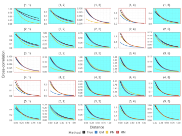
For the misspecified case of Set 1B, Figure S2 shows that GM estimates the cross-correlation function pretty well for the assumed edges (blue background) and show bias for some of the variable pairs not included in $\mathcal{G}_{\mathcal{V}}$ (white background). The accurate estimation for the covariance functions (diagonal plots) is attributable to the GGP exactly preserving the marginal distributions of the multivariate Matérn. Similarly, the estimates of the cross-covariance parameters for $(i,j)\in E_{\mathcal{V}}$ is expectedly accurate (as is concluded in Proposition 3.2).

The bias observed in estimates of the cross-correlation for some pairs of $(i,j)\notin E_{\mathcal{V}}$ is also unsurprising. The multivariate Matérn used to generate the data does not follow any graphical model or any other low-rank structure, and any form of dimension-reduction (like modelling dependencies with a sparse graph) will lead to some tradeoff in terms of accuracy and scalability. For analyzing highly multivariate spatial data, even if the variables truly doesn’t conform to any graphical model, the MM is not a feasible option due to its high-dimensional parameter space and computing requirements (Table 1) and hence dimension-reduction is necessary. Hence, using GGP with a reasonably chosen graphical model that does not exclude important variable pairs is a necessary dimension-reduction step. While it is challenging to establish a bound for the bias for excluded edges in GGP, we have proved that the marginal-preserving GGP is the information-theoretically optimal approximation of a full GP among the class of all GGP (Theorem 2.2) .

We see from Figure that S2 that the bias from GM is worse than that of PM for some $(i,j)\notin E_{\mathcal{V}}$ (e.g., $(1,4)$ or $(2,4)$). On the other hand, estimates for PM are worse for some $(i,j)\notin E_{\mathcal{V}}$ (e.g., $(1,3)$) and for a majority of the pairs $(i,i)$ and $(i,j)\in E_{\mathcal{V}}$. PM achieves dimension-reduction by imposing simplifying parameter constraints which degrades its estimation accuracy substantially for most parameters. Moreover, PM cannot even be implemented in the truly highly multivariate settings (like sets 3A and 3B) due to requiring $O(q^{3})$ for likelihood evaluation (see Table 1). The GGP offers drastic improvement in scalability over these alternatives, and for highly multivariate settings, maybe the only viable option guaranteeing accurate estimation of a large subset of the full model parameters. Additionally, we see that exclusion of edges does not severely impact the prediction quality of GM.

S3.3 Comparison with linear model of coregionalization

To compare relative performance of linear model of coregionalization and GGP in modelling low-rank processes, we consider the following simulation scenarios: (i) data is generated from an linear model of coregionalization; (ii) data is generated from a Graphical Matérn (GM) respecting the graphical model that would arise from the linear model of coregionalization in scenario (i). For each simulation setting we fit GM and linear model of coregionalization with two factor processes (using spMisalignLM function from the R package spBayes for our setting of variable-specific locations). Since spMisalignLM can be implemented only when the number of observed and latent processes are equal, for generating the data we considered two observed process based on two independent factor processes. This linear model of coregionalization leads to the graphical model from Figure 3a. Hence, for scenario (ii) we generate data from a graphical Matérn using this graph to generate correlated factor processes.

Since the two models correspond to different sets of parameters, we cannot compare them directly. Instead, in Figure S3 we compare the estimates of the entire correlation and cross-correlation functions. We observe that the impact of misspecification is more pronounced for the linear model of coregionalization; when the true model is graphical Matérn the estimate of the correlation function for the second variable by linear model of coregionalization is quite poor. In comparison, the graphical Matérn estimates the correlation and cross-correlation functions reasonably well both in the correctly specified and in the misspecified case.

(a) True process: GM

(b) True process: linear model of coregionalization

Figure S3: Estimates of cross-correlation functions for the two observed processes. The grids correspond to specific pair of the cross-correlations.

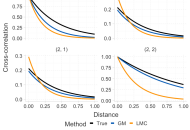
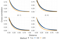
We also compare the predictive performance of the models. For all the simulations performed, we leave out $20\%$ of the data to create test sets in order to evaluate prediction accuracy of the models. Figure S4 presents the comparison of the prediction and the true values for both models and both data generation scenarios. GM reports marginally improved root mean square prediction error than linear model of coregionalization in all of the situations.

(a) True process: GM

(b) True process: linear model of coregionalization

Figure S4: Truth vs prediction for test sets in different simulation scenarios with prediction RMSE reported.

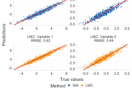
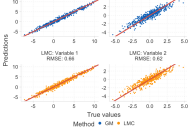
S3.4 Comparison with spatial dynamic linear models

The simulation set 3A corresponds to a highly multivariate setting ($q=100$), where the multivariate process truly follows a graphical model (path graph among the $100$ variables). None of the competing multivariate approaches besides the GGP can model such a graphical structure. These alternatives (PM and MM) also do not scale to our highly multivariate settings. In Section 4.2 we have illustrated how common univariate and multivariate spatial time-series correspond to decomposable graphical models among the variables and can be modelled using GGP. The path graph in setting 3A corresponds to the decomposable graph resulting from an AR(1) temporal structure. Hence, for this set we compare the performance of the GGP with a dynamic linear model (DLM) (Stroud et al., 2001; Gelfand et al., 2005; Finley et al., 2012) commonly used for modelling spatial time-series with AR(1) temporal evolution.

In particular, we compare GGP with the spatial dynamic linear model (SpDynLm) of Finley et al. (2012) which is set in the GP-based mixed-effect modelling setup similar to (1), as opposed to spatial basis function based approach of (Stroud et al., 2001). SpDynLM models the spatial process $w_{t}(\cdot)=w(\cdot,t)$ at time $t$ as

$$w_{t}(s)=w_{t-1}(s)+\delta_{t}(s);\quad\delta_{t}(\cdot)\sim GP(0,C_{tt}),$$ (S10)

i.e., at each time-point the spatial process is a sum of the process at the previous time point and an independent time-specific GP. The rest of the model is the same as in our setup (Eq. 1) with SpDynLM enforcing an auto-regressive evolution model for the regression coefficients $\beta_{t}$ as well.

Both SpDynLm and any GGP with a path graph between the time-specific variables model an AR(1) evolution over time. However, any DLM using an additive model of the type (S10) for the temporal evolution of the latent processes $w_{t}(c\dot{)}$, unfortunately, enforces the processes $w_{t}(\cdot)$ to have the same smoothness at all time-points $t$. Thus, even if the $\delta_{t}(\cdot)$’s are modelled using Matérn GPs with time-specific smoothness, range and variance parameters, none of the processes $w_{t}(\cdot)$ will be Matérn GPs and each will have the smoothness of the roughest of the independent processes $\delta_{t}(c\dot{)}$.

Another major restriction of the SpDynLM model is that (S10) is the customary random walk prior (Stroud et al., 2001) for $w_{t}(\cdot)$ which imposes the assumption that $\mbox{Var}(w_{t}(s))>\mbox{Var}(w_{t-1}(s))$ for all $t,s$, i.e., that the process variance is monotonically increasing over time. For most spatiotemporal processes this assumption is unlikely to hold. The GGP, on the other hand, ensures that the processes $w_{t}(\cdot)$ for each time $t$ can be modelled using a Matérn GP with time-specific variance parameters.

The dynamic model in (S10) also implicitly assumes a constant (over time) auto-regression coefficient of $1$. While this can be easily relaxed by replacing $w_{t-1}(s)$ with $\rho_{t}w_{t-1}(s)$ in (S10), the current implementation of SpDynLm does not allow modelling such a non-stationary auto-correlation coefficient $\rho_{t}$. In a GGP with a path graph, the cross-correlation parameter $b_{t,t-1}$ between the processes at two consecutive times is time-specific, thereby allowing it to capture non-stationary auto-regressive structures.

(a) Variance estimates (in log-scale).

(b) Median RMSPE over seeds for each variable (time-point).

Figure S5: Comparison between GGP and SpDynLm for modelling AR(1) spatial time series: (a) Variance estimates (in log-scale) for GM and SpDynLm compared to the true values for Set 3A. (b) Median RMSPE over seeds for each variable (time) for GM and SpDynLm for Set 3A.

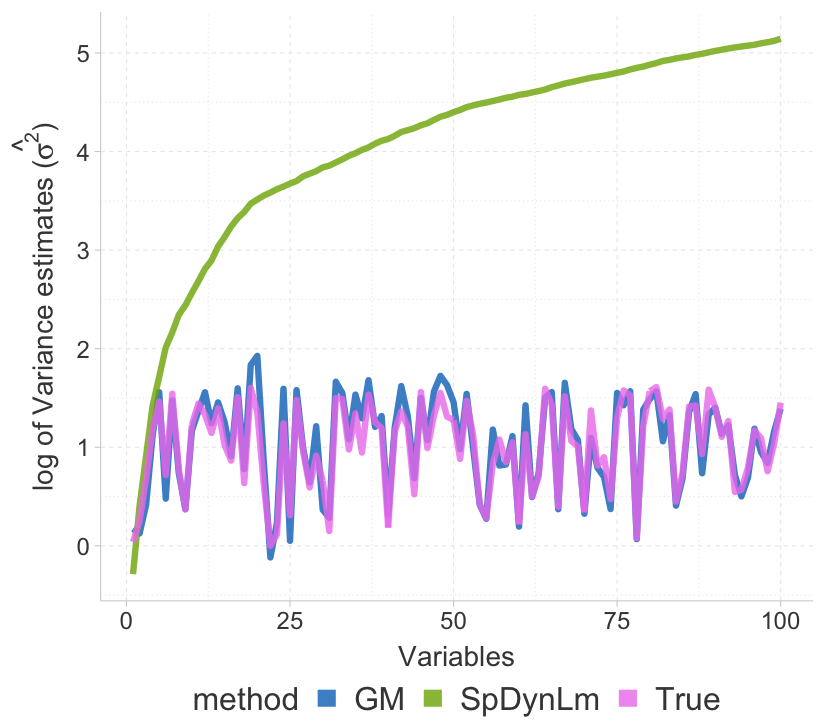
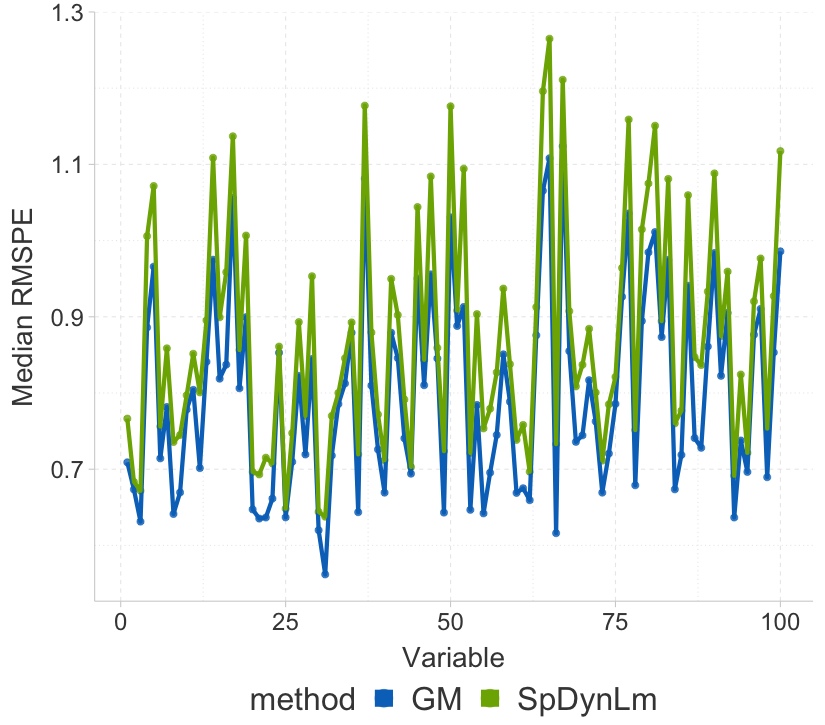
For Set 3A, the estimation accuracy of GM has already been demonstrated in Figure S1(e) (for the marginal parameters) and in Figure S9(c) (for the cross-covariance parameters representing the auto-regression). In particular, Figure S9(c) demonstrates the capability of GGP to successfully estimate non-stationary (time-specific) cross-covariance parameters. The competing model SpDynLm does not possess an autocovariance parameter that can been compared with these cross-covariances. However, we compare estimates of the marginal process variances from GGP and the SpDynLm function with the truth in Figure S5a. We observe that while GGP accurately captures the marginal variances of the processes $w_{t}(\cdot)$ for each time $t$, the estimates from SpDynLm are monotonically increasing with time and far exceeding the true values. This demonstrates the detrimental implications of the model in S10 leading to variances exploding with time and, hence, prohibiting any meaningful insight regarding the underlying processes from these parameter estimates.

We also compare the models based on their predictive performance on hold-out data. We use the implementation of SpDynLm in the SpBayes R-package (Finley et al., 2013). Figure S5b plots the median RMSPE for each variable (time-point). We see that SpDynLm produces higher predictive error (RMSPE=$0.868$) than GM (RSMPE=$0.8$) for most time-points. The numbers reported in parentheses are averaged across variables.

Overall, while predictive performance between GGP and DLM is competitive, the GGP is flexible and interpretable allowing estimation of spatial properties of the latent process $w_{t}(\cdot)$ for each time. The current implementation of SpDynLM imposes unnecessary constraints of monotonically increasing latent process variance with time leading to meaningless estimates of these parameters. More importantly, DLM assumes common smoothness over time, thereby offering no avenue to quantitatively study smoothness of the process at each time which can reveal important scientific phenomenon, e.g., pollutant surfaces can be smooth on days where the pollutant is driven by regional sources, but will be much less smooth with high local variations on days where there are significant local sources of emission.

S3.5 Comparison between different implementations of GGP

We have implemented 3 different variants of the GGP model. Besides the main focus on Bayesian model with GGP (GM) on the latent spatial processes (implementations details in Section S2.1), we have also discussed GGP on the response process (GM_response) in Section 4.5 (implementation details in Section S2.2), and have presented a frequentist estimation scheme for the parameters with maximum likelihood estimation (GM_MLE) using co-ordinate descent (see Section S2.4). In this Section we compare the performances of the 3 variants of GGP.

The MLE-based methods preclude misalignment among data locations for the different variables and excludes nugget processes $\epsilon_{i}(\cdot)$ in (1). Set 1B conforms to such assumptions. Hence, we compare GM with GM_MLE for this set. Since there is no nugget, GM and GM_response are the same for this set. Figure S6 plots the true covariance and cross-covariance parameters and their estimates from GM and GM_MLE showing that the Bayesian and frequentist implementations yield similar estimates.

(a) Set 1B (Marginal parameters)

(b) Set 1B (Cross-covariance parameters)

Figure S6: Comparison of performance of Graphical Matérn (GM) and Graphical Matérn frequentist (${\text{GM}}_{\text{MLE}}$) : (a) Estimates of the scale-covariance product parameters $\sigma_{ii}\phi_{ii}=i\in\mathcal{V}$, (b) Estimates of the cross-covariance parameters $\sigma_{ij}\phi_{ij}=\Gamma(1/2)b_{ij}$, $(i,j)\in E_{\mathcal{V}}$ for Set 1B. The horizontal pink lines in Figures (a) and (b) indicate true parameter values.

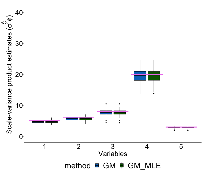
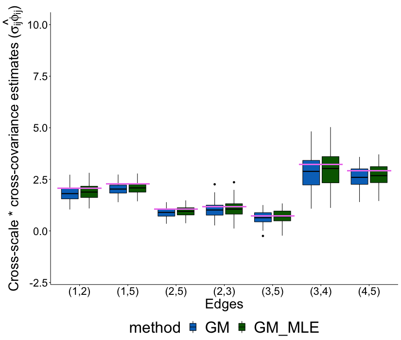
We then compare the two Bayesian implementations of GGP: GGP on the latent process (GM); and GGP on the response process (GM_response). Figure S7 plots the estimates of the covariance and cross-covariance parameters, and prediction RMSPE based on hold-out data for the two variants for Set 2B. We see that they produce similar estimates and predictive performance.

(a) Set 2B (Marginal parameters)

(b) Set 2B (Cross-covariance parameters)

(c) Set 2B (Predictions)

Figure S7: Comparison of performance of Graphical Matérn (GM) and Graphical Matérn response (${\text{GM}}_{\text{response}}$) : (a) Estimates of the scale-covariance product parameters $\sigma_{ii}\phi_{ii},i\in\mathcal{V}$, (b) Estimates of the cross-covariance parameters $\sigma_{ij}\phi_{ij}=\Gamma(1/2)b_{ij}$, $(i,j)\in E_{\mathcal{V}}$ and (c) median RMSPE for Set 2B. The horizontal pink lines in Figures (a) and (b) indicate true parameter values.

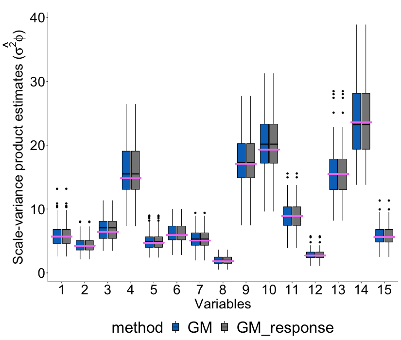
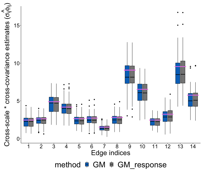
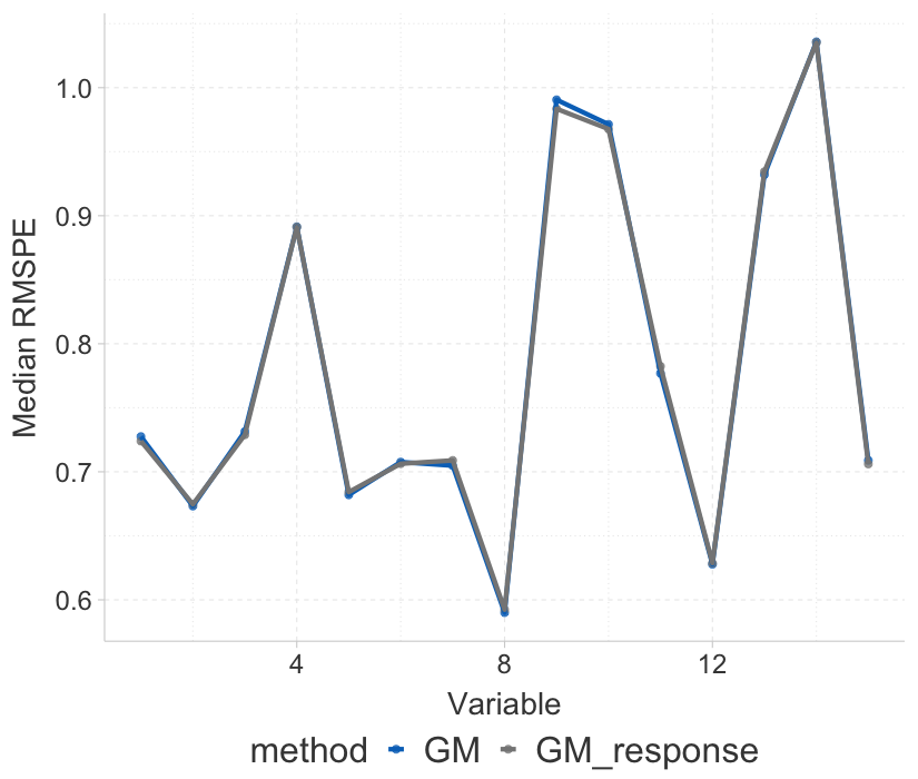
S4 Additional figures and tables

(a) DAG for a univariate AR(2) model

(b) Moralized $\mathcal{G}_{\mathcal{T}}$ for a univariate AR(2) model

(c) DAG for the graphical VAR model example of Section 4.2

(d) Moralized $\mathcal{G}_{\mathcal{V}\times\mathcal{T}}$ for the graphical VAR model of Figure (c)

Figure S8: Graphical models for autoregressive spatial time-series.

(a) Set 1A

(b) Set 2A

(c) Set 3A

Figure S9: Estimation performance of graphical Matérn in the correctly specified case: (a), (b) and (c): Estimates of the cross-covariance parameters $\sigma_{ij}\phi_{ij}=\Gamma(1/2)b_{ij}$, $(i,j)\in E_{\mathcal{V}}$ for the 3 simulation sets (1A, 2A and 3A) where the graphical Matérn is correctly specified. The horizontal pink lines in Figures (a) and (b) indicate true parameter values.

(a) Posterior edge selection probabilities for Set 1A.

(b) Cross-covariance parameter estimates for Set 1A while estimating the unknown graph

Figure S10: Performance of GGP with unknown graph for Set 1A: (a): Marginal edge probabilities estimated from the reversible jump MCMC sampler. Blue edges denote the true edges and red denotes the non-existent edges. Edges are weighted proportional to the estimated posterior selection probabilities. (b) GM estimates of cross-correlation parameters ($b_{ij}$) corresponding to true edges when the graph is unknown.

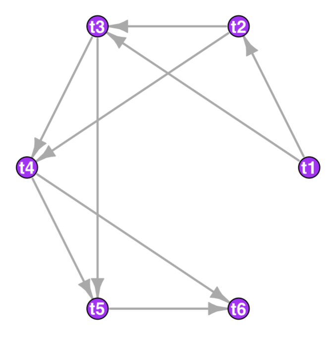
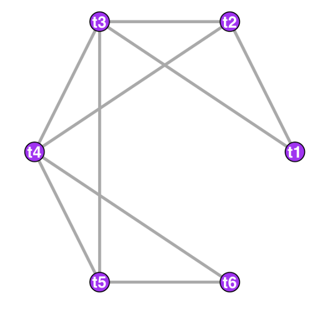
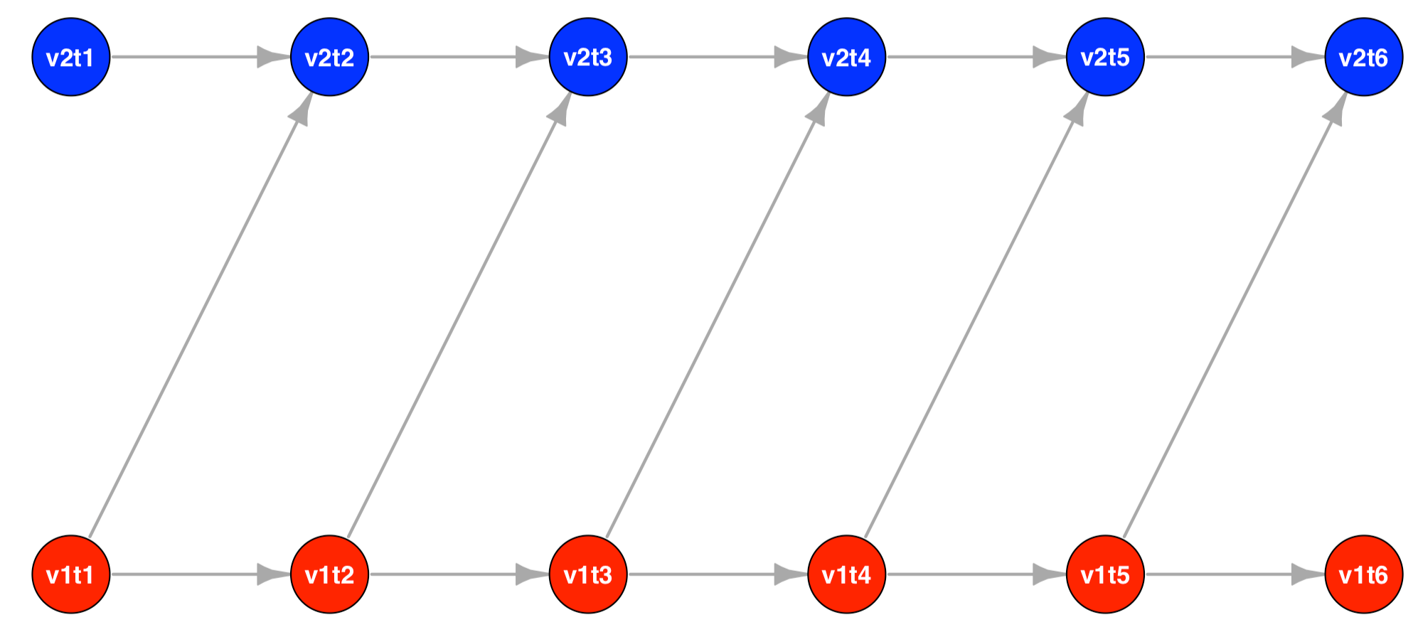
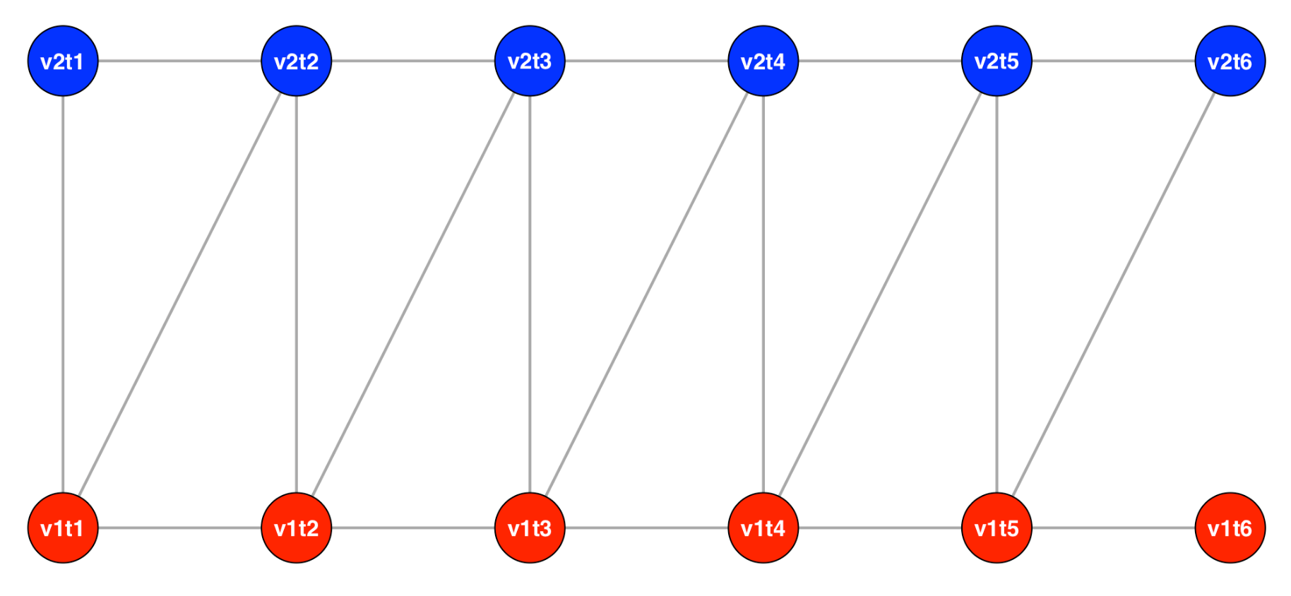
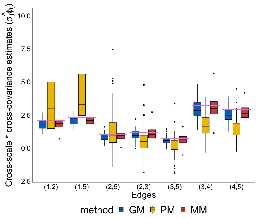
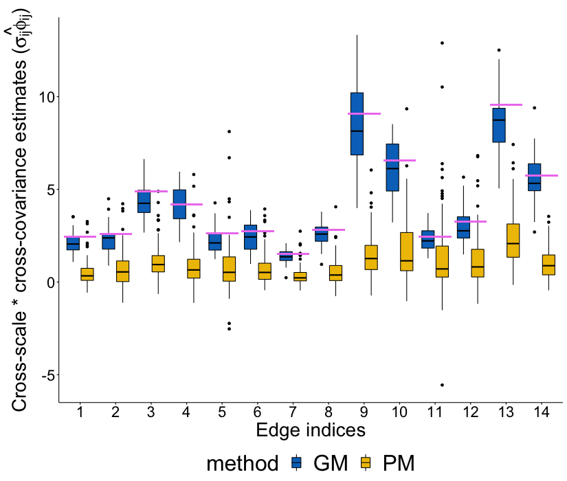
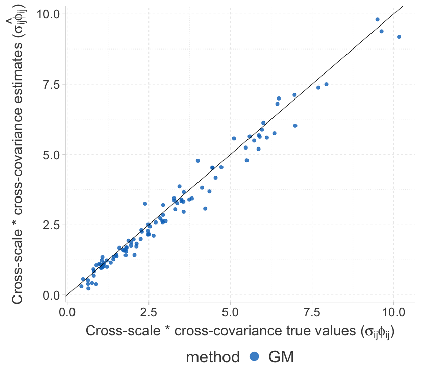
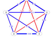
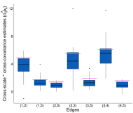
Set 1A (True = Gem graph)		Set 2A (True = Path graph)
Edges	Probability	Edges	Probability
(3, 4)	0.64	(1, 2)	0.43
(1, 2)	0.57	(11, 12)	0.42
(1, 5)	0.57	(2, 3)	0.42
(2, 3)	0.55	(14, 15)	0.41
(2, 5)	0.50	(4, 5)	0.40
(3, 5)	0.48	(7, 8)	0.38
(4, 5)	0.46	(8, 9)	0.37
(1, 3)	0.45	(13, 14)	0.34
(2, 4)	0.43	(6, 7)	0.33
(1, 4)	0.42	(10, 11)	0.32
		(9, 10)	0.31
		(5, 6)	0.30
		(12, 13)	0.30
		(3, 4)	0.27
		(1, 3)	0.22
		(13, 15)	0.21
		(9, 11)	0.20
		(7, 9)	0.18
		(4, 6)	0.18
		(10, 12)	0.18

Table S3: Posterior probabilities of including an edge when estimating the graph in a GGP. The rows of the table are ordered from highest to lowest. (a) Set 1A (all edges), (b) Set 2A (edges with the top 20 highest selection probabilities). Bold numbers indicate true edges.

Figure S11: Truth vs prediction for test set data compared among GM and SpDynLM

Figure S12: Density of residual spatial process values (across locations) for two different time periods - first two weeks of February and last two weeks of April

References

- Apanasovich & Genton (2010) Apanasovich, T. V. & Genton, M. G. (2010). Cross-covariance functions for multivariate random fields based on latent dimensions. Biometrika 97, 15–30.
- Apanasovich et al. (2012) Apanasovich, T. V., Genton, M. G. & Sun, Y. (2012). A valid Matérn class of cross-covariance functions for multivariate random fields with any number of components. Journal of the American Statistical Association 107, 180–193.
- Atay-Kayis & Massam (2005) Atay-Kayis, A. & Massam, H. (2005). A Monte Carlo method for computing the marginal likelihood in nondecomposable Gaussian graphical models. Biometrika 92, 317–335.
- Banerjee et al. (2014) Banerjee, S., Carlin, B. P. & Gelfand, A. E. (2014). Hierarchical Modeling and Analysis for Spatial Data. Boca Raton, FL: Chapman & Hall/CRC, 2nd ed.
- Banerjee et al. (2008) Banerjee, S., Gelfand, A. E., Finley, A. O. & Sang, H. (2008). Gaussian predictive process models for large spatial data sets. Journal of the Royal Statistical Society: Series B (Statistical Methodology) 70, 825–848.
- Barker & Link (2013) Barker, R. J. & Link, W. A. (2013). Bayesian multimodel inference by RJMCMC: A Gibbs sampling approach. The American Statistician 67, 150–156.
- Cox & Wermuth (1996) Cox, D. R. & Wermuth, N. (1996). Multivariate Dependencies: Models, Analysis and Interpretation. Chapman and Hall/CRC.
- Cramér (1940) Cramér, H. (1940). On the theory of stationary random processes. Annals of Mathematics , 215–230.
- Cressie & Zammit-Mangion (2016) Cressie, N. & Zammit-Mangion, A. (2016). Multivariate spatial covariance models: a conditional approach. Biometrika 103, 915–935.
- Cressie & Wikle (2011) Cressie, N. A. C. & Wikle, C. K. (2011). Statistics for spatio-temporal data. Wiley Series in Probability and Statistics. Hoboken, NJ: Wiley.
- Dahlhaus (2000) Dahlhaus, R. (2000). Graphical interaction models for multivariate time series. Metrika 51, 157–172.
- Dahlhaus & Eichler (2003) Dahlhaus, R. & Eichler, M. (2003). Causality and graphical models in time series analysis. Oxford Statistical Science Series , 115–137.
- Datta et al. (2016) Datta, A., Banerjee, S., Finley, A. O. & Gelfand, A. E. (2016). Hierarchical nearest-neighbor Gaussian process models for large geostatistical datasets. Journal of the American Statistical Association 111, 800–812.
- Datta et al. (2019) Datta, A., Banerjee, S., Hodges, J. S. & Gao, L. (2019). Spatial disease mapping using directed acyclic graph auto-regressive (DAGAR) models. Bayesian analysis 14, 1221.
- Dempster (1972) Dempster, A. P. (1972). Covariance selection. Biometrics , 157–175.
- Dobra et al. (2003) Dobra, A. et al. (2003). Markov bases for decomposable graphical models. Bernoulli 9, 1093–1108.
- Eichler (2008) Eichler, M. (2008). Testing nonparametric and semiparametric hypotheses in vector stationary processes. Journal of Multivariate Analysis 99, 968–1009.
- Eichler (2012) Eichler, M. (2012). Fitting graphical interaction models to multivariate time series. arXiv:1206.6839 .
- Finley et al. (2012) Finley, A. O., Banerjee, S. & Gelfand, A. E. (2012). Bayesian dynamic modeling for large space-time datasets using Gaussian predictive processes. Journal of geographical systems 14, 29–47.
- Finley et al. (2013) Finley, A. O., Banerjee, S. & Gelfand, A. E. (2013). spbayes for large univariate and multivariate point-referenced spatio-temporal data models. arXiv:1310.8192 .
- Finley et al. (2009) Finley, A. O., Sang, H., Banerjee, S. & Gelfand, A. E. (2009). Improving the performance of predictive process modeling for large datasets. Computational statistics & data analysis 53, 2873–2884.
- Gelfand et al. (2005) Gelfand, A. E., Banerjee, S. & Gamerman, D. (2005). Spatial process modelling for univariate and multivariate dynamic spatial data. Environmetrics 16, 465–479.
- Gelfand et al. (2004) Gelfand, A. E., Schmidt, A. M., Banerjee, S. & Sirmans, C. (2004). Nonstationary multivariate process modeling through spatially varying coregionalization. Test 13, 263–312.
- Genton & Kleiber (2015) Genton, M. G. & Kleiber, W. (2015). Cross-covariance functions for multivariate geostatistics. Statistical Science , 147–163.
- Gneiting (2002) Gneiting, T. (2002). Nonseparable, stationary covariance functions for space–time data. Journal of the American Statistical Association 97, 590–600.
- Gneiting et al. (2010) Gneiting, T., Kleiber, W. & Schlather, M. (2010). Matérn cross-covariance functions for multivariate random fields. Journal of the American Statistical Association 105, 1167–1177.
- Gonzalez et al. (2011) Gonzalez, J., Low, Y., Gretton, A. & Guestrin, C. (2011). Parallel Gibbs sampling: From colored fields to thin junction trees. In Proceedings of the Fourteenth International Conference on Artificial Intelligence and Statistics.
- Green & Thomas (2013) Green, P. J. & Thomas, A. (2013). Sampling decomposable graphs using a Markov chain on junction trees. Biometrika 100, 91–110.
- Heaton et al. (2019) Heaton, M. J., Datta, A., Finley, A. O., Furrer, R., Guinness, J., Guhaniyogi, R., Gerber, F., Gramacy, R. B., Hammerling, D., Katzfuss, M. et al. (2019). A case study competition among methods for analyzing large spatial data. Journal of Agricultural, Biological and Environmental Statistics 24, 398–425.
- Jacquier et al. (1993) Jacquier, E., Polson, N. & Rossi, P. (1993). Priors and models for multivariate stochastic volatility. Unpublished manuscript, Graduate School of Business, University of Chicago .
- Jacquier et al. (2002) Jacquier, E., Polson, N. G. & Rossi, P. E. (2002). Bayesian analysis of stochastic volatility models. Journal of Business & Economic Statistics 20, 69–87.
- Jung et al. (2015) Jung, A., Hannak, G. & Goertz, N. (2015). Graphical lasso based model selection for time series. IEEE Signal Processing Letters 22, 1781–1785.
- Kleiber (2017) Kleiber, W. (2017). Coherence for multivariate random fields. Statistica Sinica , 1675–1697.
- Lauritzen (1996) Lauritzen, S. L. (1996). Graphical models, vol. 17. Clarendon Press.
- Li & Zhang (2011) Li, B. & Zhang, H. (2011). An approach to modeling asymmetric multivariate spatial covariance structures. Journal of Multivariate Analysis 102, 1445–1453.
- Lopes et al. (2008) Lopes, H. F., Salazar, E. & Gamerman, D. (2008). Spatial dynamic factor analysis. Bayesian Analysis 3(4), 759 – 792.
- Parra & Tobar (2017) Parra, G. & Tobar, F. (2017). Spectral mixture kernels for multi-output Gaussian processes. In Advances in Neural Information Processing Systems.
- Ren & Banerjee (2013) Ren, Q. & Banerjee, S. (2013). Hierarchical factor models for large spatially misaligned data: A low-rank predictive process approach. Biometrics 69, 19–30.
- Roverato (2002) Roverato, A. (2002). Hyper inverse Wishart distribution for non-decomposable graphs and its application to Bayesian inference for Gaussian graphical models. Scandinavian Journal of Statistics 29, 391–411.
- Saha et al. (2021) Saha, A., Basu, S. & Datta, A. (2021). Random forests for spatially dependent data. Journal of the American Statistical Association , 1–46.
- Saha & Datta (2018) Saha, A. & Datta, A. (2018). BRISC: bootstrap for rapid inference on spatial covariances. Stat 7, e184.
- Schmidt & Gelfand (2003) Schmidt, A. M. & Gelfand, A. E. (2003). A Bayesian coregionalization approach for multivariate pollutant data. Journal of Geophysical Research: Atmospheres 108.
- Speed et al. (1986) Speed, T. P., Kiiveri, H. T. et al. (1986). Gaussian Markov distributions over finite graphs. The Annals of Statistics 14, 138–150.
- Stroud et al. (2001) Stroud, J. R., Müller, P. & Sansó, B. (2001). Dynamic models for spatiotemporal data. Journal of the Royal Statistical Society: Series B (Statistical Methodology) 63, 673–689.
- Taylor-Rodriguez et al. (2019) Taylor-Rodriguez, D., Finley, A. O., Datta, A., Babcock, C., Andersen, H.-E., Cook, B. D., Morton, D. C. & Banerjee, S. (2019). Spatial factor models for high-dimensional and large spatial data: An application in forest variable mapping. Statistica Sinica 29, 1155.
- Thomas & Green (2009) Thomas, A. & Green, P. J. (2009). Enumerating the junction trees of a decomposable graph. Journal of Computational and Graphical Statistics 18, 930–940.
- Wackernagel (2013) Wackernagel, H. (2013). Multivariate geostatistics: an introduction with applications. Springer Science & Business Media.
- Wang & West (2009) Wang, H. & West, M. (2009). Bayesian analysis of matrix normal graphical models. Biometrika 96, 821–834.
- Xu et al. (2011) Xu, P.-F., Guo, J. & He, X. (2011). An improved iterative proportional scaling procedure for Gaussian graphical models. Journal of Computational and Graphical Statistics 20, 417–431.
- Zhang & Banerjee (2021) Zhang, L. & Banerjee, S. (2021). Spatial factor modeling: A Bayesian matrix-normal approach for misaligned data. Biometrics .