Is Factor Momentum More than Stock Momentum?
††thanks: We are especially grateful to Jean-Philippe Bouchaud for his feedback. We also thank Mark Potters, Philip Seager, as well as CFM seminar participants for useful comments.
Abstract
Yes, but only at short lags. In this paper we investigate the relationship between factor momentum and stock momentum. Using a sample of 72 factors documented in the literature, we first replicate earlier findings that factor momentum exists and works both directionally and cross-sectionally. We then ask if factor momentum is spanned by stock momentum. A simple spanning test reveals that after controlling for stock momentum and factor exposure, statistically significant Sharpe ratios only belong to implementations which include the last month of returns. We conclude this study with a simple theoretical model that captures these forces: (1) there is stock-level mean reversion at short lags and momentum at longer lags, (2) there is stock and factor momentum at all lags and (3) there is natural comovement between the PNLs of stock and factor momentums at all horizons.
1 Introduction
This paper analyzes factor momentum. In recent years, a body of literature in asset pricing has analyzed the properties of a large number of risk factors (Harvey and Zhu (2016), McLean and Pontiff (2016), Hou and Zhang (2019), Giglio et al. (2020)). These factors are constructed by sorting stocks along various characteristics and are evidence that stock returns are predictable and co-move. As it turns out, recent research suggests that factor returns are themselves predictable (Cohen et al. (2003),Haddad et al. (2020)) and in particular exhibit momentum (Ehsani and Linnainmaa, 2019): A factor that was performing well tends to perform well in the future. At the same time, it has been known for long that stocks also exhibit momentum (Jegadeesh and Titman (1993)). Factor and stock momentum are likely to be interconnected: Since stocks are exposed to factors, and factors have persistent returns, factor momentum may explain stock momentum. Conversely, since factors are portfolio of stocks, stock momentum may mechanically lead to factor momentum. This paper investigates the relation between these two momentums. We find that factor momentum is difficult to distinguish from stock momentum: The only difference is at monthly time scale, where stocks mean revert while factors exhibit strong momentum.
We shall proceed in three steps. First, we use US data and build a dataset that contains 72 documented signals published in the literature. We replicate the construction of factors as long-short dollar-neutral portfolios and further hedge their residual market exposure dynamically. An equal-risk average of these factors generates a Sharpe ratio of 0.96, thereby confirming the soundness of our replication exercise. Consistent with many investment strategies becoming crowded over time, we find that average risk-adjusted performance tends to taper off in the late 2000s. We then document that these factors exhibit momentum. As Ehsani and Linnainmaa (2019), we explore both types of factor momentum: cross-sectional (buying the most successful factors and selling the least performing ones) and directional (buying factors with past positive returns and selling factors with past negative returns). We find that both strategies deliver significant and similar risk-adjusted performance, with a Sharpe ratio around 1. We then analyze “mechanical” drivers of factor momentum. Since factor momentum buys the best performing factors and sells the unperforming ones, factor momentum contains a mechanical exposure to the mean and spread of factor returns, a phenomenon shown in Lo and MacKinlay (1990). Controlling for mean factor return, we still find that factor momentum is present, in line with results shown by Ehsani and Linnainmaa (2019) using a different set of factors and a slightly different spanning approach. The bottom line is that factor momentum is a resilient anomaly that begs for an explanation.
In the second step of our analysis, we analyze the distinction between factor and stock momentum. We use the following approach. In the spirit of Jegadeesh and Titman (1993)’s analysis of stock momentum, we analyze a full range of definitions of factor momentum using various lags (how many most recent months of data one discards when constructing the signal) and various “holding periods” (number of months worth of stock returns used to compute momentum). We first find that factor momentum is present for a large range of lags and holding periods. We then compute the excess performance of each one of these momentums after controlling for factor exposure. Consistently with our first step, we find that controlling for mean factor exposure removes about 0.2 points of Sharpe from all factor momentums (i.e., irrespective of lag and holding period). Controlling for stock momentum further reduces the Sharpe of nearly all factor strategies, except for the smallest possible lag (one month). Further, the excess return remains particularly strong when one focuses on one-month lag and one-month momentum time scale, i.e., the monthly mean reversion. Additional analysis confirms that factor momentum is “spanned” by stock momentum and factor exposure, except at one-month time scale. Put differently, factor returns are persistent at the monthly time scales, while stock returns mean revert. Otherwise, factor momentum is not distinguishable from stock momentum.
In our third step we develop a simple model designed to encapsulate these findings. The key question is whether factor momentum can co-exist with stock mean reversion at short horizons and stock momentum at longer horizons. In our model there are three types of investors: noise traders, positive feedback traders who buy stocks exposed to an arbitrary factor when it performs well and contrarian traders, who buy stocks whose price is high. The model captures the three features present in the data: (1) there is stock-level mean reversion at short lags and momentum at longer lags, (2) there is factor momentum at all lags and (3) there is natural comovement between the PNLs of stock and factor momentums at all horizons (short- and long-term).
Our paper contributes to the literature on factor timing. This literature looks for evidence that risk factor returns are themselves predictable. Most papers in this space focus on mean-reversion in factor returns. Cohen et al. (2003), and more recently Haddad et al. (2020) build on the idea that factors are measures of risk premia, which tend to be mean-reverting (Campbell and Shiller, 1987): A factor is expensive when stocks in its long (short) leg have a high (low) market to book ratio. Both papers find evidence consistent with the idea that expensive factors tend to have lower future returns. Cohen et al. (2003) focuses on the value premium, while Haddad et al. (2020) focus on the first PCs of a large group of factors. In the same spirit, Hanson and Sunderam (2014) find that factors that short stocks that are otherwise heavily shorted tend to mean revert.
Our paper focuses instead on shorter-term persistence in factor returns. We follow Ehsani and Linnainmaa (2019) and provide further evidence of factor momentum using a different set of factors (we have 72 factors while they have 20 in their baseline study; moreover our factors are defined in US only) and a slightly different portfolio construction. Like these authors, we find that directional factor momentum is marginally stronger than the cross-sectional implementation, with both strategies generating most of their returns from their long legs. But the main difference between their study and ours is in the test differentiating stock and factor momentum. They construct factor momentum as a strategy based on the past 12 months of returns, while stock momentum is also based on the past 12 months of returns excluding the last month. They find that factor momentum is not spanned by stock momentum. Our strategy consists of looking at different definitions of factor momentum, where we vary both the lag and the holding period. This allows us to uncover the source of the discrepancy between the two momentums: At one-month time scales, stocks mean-revert while factors have persistent returns. If we exclude the last month of returns, factor momentum is subsumed by stock momentum. We provide a model consistent with our findings.
The paper is structured as follows. Section 2 describes the data and the construction of our factor zoo. Section 3 provides evidence of factor momentum and tests for mechanical drivers of momentum. Section 4 decomposes factor momentum into various lags and horizons. This decomposition shows the key role of the lag in differentiating between both types of momentum. Finally, Section 5 proposes a model consistent with stylized facts that we uncovered. Section 6 concludes.
2 Data & Factor Construction
We construct time series of returns for 72 risk factors documented in the literature (see list in Appendix A). These risk factors use data from a CRSP-COMPUSTAT merged sample, so they only use accounting and price information. This sample runs from January 1963 to April 2014. In our merger of CRSP and COMPUSTAT, we make sure that there is no look ahead bias in financial statement availability. We assume that financial statements for the last fiscal year become available four months later. This is conservative as earnings are typically anounced between 2 and 3 months after the end of the fiscal year. But it ensures that there is little look ahead bias in our data.
While our implementation of the 72 sorting variables is faithful to the papers we replicate, we propose certain improvements to risk management in order to be closer to what is common practice in asset management. First, we restrict our analysis to the 1,000 most liquid stocks on CRSP. This is in order to ensure that the factors trade liquid stocks and have reasonable capacity. Second, we construct and risk manage each factor using the following methodology. For each factor in Appendix A, we first compute daily factor returns by implementing the characteristic proposed in the original factor paper and using the portfolio construction method proposed by the authors. We resample the PnLs monthly. Next, we remove any residual exposure to being long the market by beta-hedging, i.e. we run a rolling 36 months regression of the factor PnL onto market returns to determine the (past) beta and use this beta for the following month to debias PnLs. Finally, we risk manage the resulting PnL by dividing it by the (rolling) standard deviation of returns computed over past 36 months and lagged one month. This ensures that each beta-hedged factor PnL has a relatively constant volatility and is thus closer to how factor investing would be implemented in practice. We report the distribution of Sharpe ratios and t-stats of our 72 factors in Table 1. As it becomes apparent, a typical factor Sharpe ratio is low (0.27), suggesting potential overfitting or arbitrage, an issue we explore in a companion paper.
| Mean | Median | p25 | p75 | |
|---|---|---|---|---|
| Annualized Sharpe | 0.27 | 0.35 | -0.02 | 0.55 |
| t stat | 1.73 | 2.11 | -1.25 | 3.64 |
Note: Annualised Sharpe and t stats, computed with monthly returns. All factor are beta-neutralised and risk-managed, computed on CRSP 1,000 most liquid stocks from 1963 to 2014.
We report in Figure 1 the cumulative return of factor risk-parity. This investment strategy consists in being long an equal amount of risk of each of the 72 factors and is run at a constant overall risk target. In what follows, we will refer to this strategy per “menagerie” (all of the “animals” in our “zoo” of factors). The Sharpe ratio of this strategy over the entire period is 0.96. The cumulative return does however show signs of tapering off starting in the mid 2000s. This is consistent with the idea, described in McLean and Pontiff (2016) among others, that after publication the strategies listed in these papers perform less well.
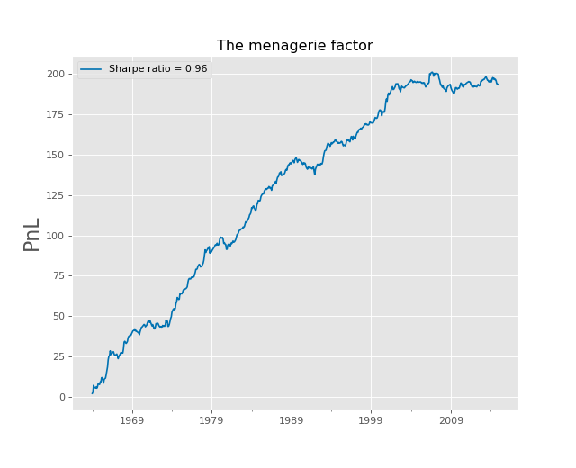
We report here the cumulative return of factor risk parity with 72 factors. The investment strategy is beta-hedged in order to filter out exposure to the market and run at a constant risk target.
3 Evidence on Factor Momentum
3.1 Defining momentum
Let be a vector of monthly factor returns, with returns computed between months and (and each factor constructed using information available at ). Each component of this vector corresponds to one of our risk-managed factors presented in Section 2, i.e. they are dynamically hedged with respect to market exposure and scaled by rolling volatility. is the number of components. We first define the “menagerie” as investing $1 in each one of these factors (so the amount of risk in each factor is the same). Hence the PNL of the menagerie at the end of month is:
where is a vector of ones. We denote the transpose by ′.
We then define cross-sectional and directional factor momentum as in Ehsani and Linnainmaa (2019). The key difference is that we sort factors based on past returns computed from to . Put differently, is the most recent price used (the “lag”) and is the number of months used (the “holding period”). To make things clear, we note:
the cumulative return between and . Note that as a special case .
The PNL of cross-sectional factor momentum is given by:
| (1) |
where the rank operator transforms a vector with components into a vector of ranks with different, equally-spaced components in the range . By construction the cross-sectional momentum is always dollar neutral, i.e. the sum of weights is equal to zero.
The PNL of directional momentum does not impose dollar neutrality. We define it as:
| (2) |
For instance, if all factors have performed positively in the past period, the factor momentum portfolio will (temporarily) be the same as the menagerie. The net leverage of this strategy varies over time: it increases (decreases) when factors have positive (negative) returns.
The above definitions (menagerie, XS and TS momentum) are that of “raw” portfolios, in the sense that they are not risk managed. The empirical results we present below are for the “risk-managed” versions of these PNLs, which are obtained by normalizing the returns with their rolling 36 month volatility lagged one month. Remember that each one of the factors is itself already risk-managed.
Last, for clarity of exposition, we focus in the sections that follow on directional momentum, but our results with cross-sectional momentum are very similar. We report them in Appendix B.
3.2 Factor Momentum: First Evidence
Here, we redo the analysis in Ehsani and Linnainmaa (2019) using our own set of factors and report results in Table 2. The first line shows the performance of the menagerie strategy, which has a Sharpe ratio of 0.96 (as we showed in Figure 1) and a t-stat of 6.86.
| Sharpe ratio | -value | |
|---|---|---|
| Menagerie | 0.96 | 6.86 |
| TS | 1.16 | 8.22 |
| TS, winners | 1.29 | 9.11 |
| TS, losers | 0.43 | 3.03 |
| XS | 1.01 | 7.12 |
| XS, winners | 1.20 | 8.52 |
| XS, losers | 0.46 | 3.24 |
Note: Annualised statistics computed with monthly returns. We compute factor momentum signals using and . Factors are beta-neutralised and risk-managed, computed on CRSP 1,000 most liquid stocks from 1963 to 2014.
The next lines of Table 2 show the performance of factor momentum. We calculate the direct returns of cross-sectional and directional momentum (using formulas (1) and (2)). We set and for now (we come back to varying and later). Time series and cross-sectional momentum both have high Sharpe ratios and the directional implementation outperforms the cross-sectional one by in Sharpe. Ehsani and Linnainmaa (2019) also find that directional factor momentum outperforms, but they find a somewhat larger difference in Sharpe .26 (Their Table 2). There are three main differences between their methodology and ours. First, we are using a larger set of factors. Second, we are constructing our factors using the 1,000 largest U.S. stocks only. Our construction thus excludes illiquid microcaps. Last, we risk-manage and beta-neutralize factors’ PNLs. In spite of these significant differences, we manage to reproduce their headline results quite closely.
Another salient feature of Table 2 is that most of the return on factor momentum is borne by the long leg of the strategy (the “winners”). Ehsani and Linnainmaa (2019) find similar results. One possibility is that this whole effect is driven by somewhat unsophisticated, long-biased investors piling into factors that performed well, as in Hanson and Sunderam (2014)). We rely on this idea in our model of Section 5.
3.3 Accounting for mechanical exposure of momentum to factors
The key role of the long leg of factor momentum also suggests that part of the performance may simply come from outright exposure to factors. This concern is particularly relevant for directional momentum. This intuition can easily be confirmed in a momentum decomposition à la Lo and MacKinlay (1990). Let us focus on one single factor (an element of ). Assume that this factor follows an AR1 process , where is the long-run excess return of the factor. Then, the conditional and unconditional PNLs of directional momentum on this factor alone are given by:
These two formulas illustrate why factor momentum is more likely to have a good PNL if the expected return of the factor is positive , independently of the strength of factor momentum itself (). To fix ideas, set . The first equation shows the conditional PNL of the factor momentum strategy, which is non-zero. Indeed when the factor has performed well (), the momentum trader will purchase it and will thus cash in the expected premium : expected profit will be , even though factor returns have no real momentum. Another way to see this is by looking at the unconditional PNL in the second equation. Even if , and as long as , factor momentum always generates a positive PNL. On average, factors with positive premia are more likely to experience two consecutive dates of positive returns. All the same, factors with negative premia are more likely to underperform on two consecutive dates. This ensures even if there is no actual persistence in returns.
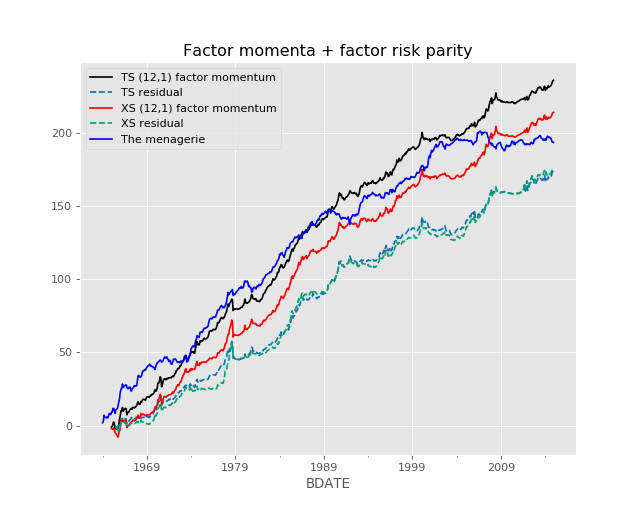
Cumulative sum of returns to two factor momentum strategies and the menagerie factor. All PnLs are rescaled (in a causal way) to target 1% monthly volatility. Factors are beta-neutralised and risk-managed, computed on CRSP 1,000 most liquid stocks from 1963 to 2014.
To account for this mechanical relationship (and isolate the pure effect of factor momentum), we look at the residual of the regression of factor momentum PNL on the menagerie PNL. The regression is run over the entire period as we are not looking to hedge factor momentum, but rather to measure its de facto exposure to the menagerie. We show the effect of this control in Figure 2 where we report the momentum returns alongside with the corresponding residuals. We can see that the cumulative PNLs of residuals are about 20% less than that of pure factor momentum. Thus, while the mechanical exposure of momentum to factor returns in non-negligible, factor momentum remains a strong force.
4 Factor vs Stock Momentum
We now turn to the analysis of the link between stock momentum and factor momentum. We start with an analysis of the correlation between the two factors. We then break the analysis down into various lags and holding periods. In this section we use the directional implementation of factor momentum. The results for cross-sectional momentum are similar and are reported in Appendix B.
4.1 Correlation with Stock Momentum assuming standard lag and holding period
To investigate this, a natural object to look at is the correlation between stock and factor momentum. Let us first investigate this correlation analytically. To fix ideas, let us assume that the vector of stock returns (between period and ) follows a single factor structure:
where is a vector of factor exposures of individual stocks and is the idiosyncratic shock, assumed to be stationary, i.i.d. and most importantly independent of for all lags. The factor can be persistent but we assume it to be homoskedastic – its conditional variance does not vary with time. We define here the PNLs of (directional) factor and stock momentum strategies as:
where the lower bars stand for lagged cumulative returns with arbitrary lag and holding period . In this section we do not risk manage PNLs in order to obtain closed-form formulas (in the empirical analysis we will stick with the empirical definitions).
In this setting one can show (See Appendix C.1) that the covariance between the two PNLs is given by:
| (3) |
which is generally positive, whether factor momentum has a positive PNL or not. The intuition is simple: Buying winning stocks is equivalent to exposing oneself to the factor. So whenever stock momentum performs well, it is likely that the underlying factor has performed well. In this very simple setup, all of stock momentum comes from factor momentum (as we assumed to be i.i.d.). So even if factor momentum is not present, there will be instances when it works by accident and consequently stock momentum will work too. The bottom line of this analysis is that the covariance between both strategies is mechanically positive, even when none of them has a positive Sharpe ratio. This due to the fact that is stable.
Let us now move to the empirical analysis and compute the correlation between the two types of momentum. For factor momentum, we choose and . For stock momentum, we use UMD, the stock momentum factor available from the Fama-French data library. UMD sets and in order to exclude short-term mean-reversion. We report this correlation and other statistics in Table 3. We use monthly returns. As expected from our algebra, the correlation of factor momentum with UMD is high, around 60%. This is much higher than the correlation between UMD and the menagerie (0.04%). Note that this high correlation is thus unaffected whether we look at directional, cross-sectional or residual momentum. The analysis above has shown why part of this correlation is likely to be mechanical.
| Menagerie | Menagerie w/o UMD | TS | TS residual | XS | XS residual | |
| Correlation | 0.04 | -0.08 | 0.57 | 0.59 | 0.58 | 0.58 |
Factors are beta-neutralised, risk-managed and computed on CRSP 1,000 most liquid stocks from 1963 to 2014. UMD sorts stocks based on the last 12 months of returns except for the most recent one ( and ). XS and TS factor momentum sorts factors using the last 12 months of returns ( and ).
This very strong correlation between the two types of momentum begs for a “spanning test”. To do this we regress the PNL of factor momentum on the PNL of the stock momentum strategy using the entire sample. We then compute the Sharpe ratio of the residual strategy. Using the above definitions of stock and factor momentum we find a Sharpe ratio of 0.59, which is statistically significant. We explore this in greater detail in Section 4.3. The fact that stock momentum does not entirely span factor momentum is consistent with Ehsani and Linnainmaa (2019) who implement similar spanning tests . This analysis is, however, incomplete as (1) it does not take into account mechanical exposure to the menagerie (as shown in Section 3.3) and (2) the lags are different for stock and factor momentum. Let us now investigate these two aspects.
4.2 Performance of stock and factor momentum for different lags and holding periods
In this section we vary the holding period and the lag and control for their values when analyzing the correlation between the two types of momentum. It is a priori important to control for these parameters, as they greatly affect the performance of momentum, as it is well known since at least Jegadeesh and Titman (1993).
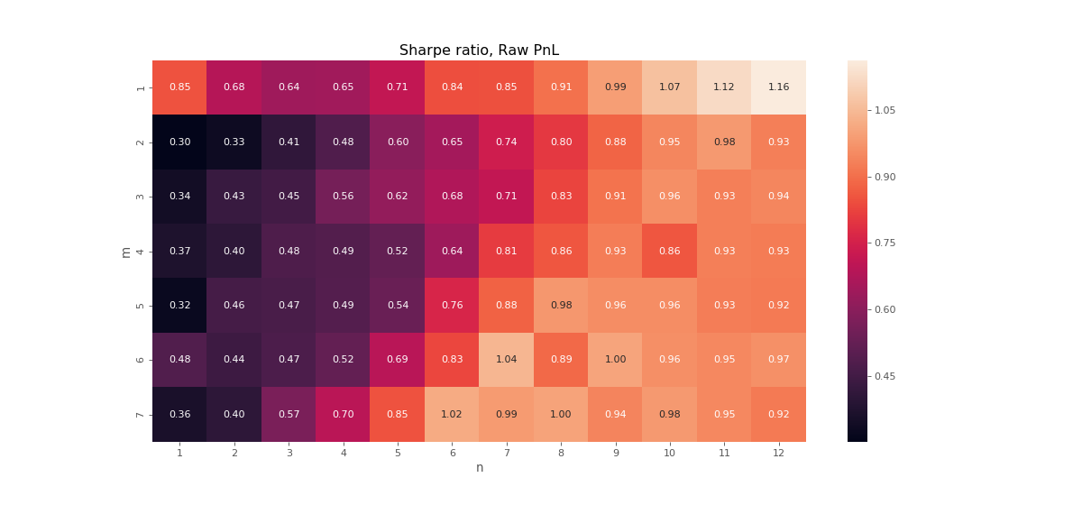
In Figure 3, before looking at correlations, we first show the performance of both strategies for different values of and . Panel A focuses on stock momentum and reproduces three classical results . First, there is short term reversal for as evidenced by the very dark cells (indicating negative Sharpe of momentum) in the upper left corner of the heat map. Second, the classic momentum (, ) has a high Sharpe ratio (0.8). Third, a strongly lagged momentum (, ) has an impressive Sharpe ratio, around 1 as previously noticed by Novy-Marx (2012). Put differently, there is a northeast-southwest diagonal of light colors on the right side of the heat map, which is an evidence of the strength of “lagged momentum”. In panel B we focus on factor momentum. Two salient patterns emerge. First, there is no short-term reversal in factor returns. Past factor returns always predict stronger future returns, even at short time scales. It is clear that having the most recent month of return increases the performance of the strategy: A big fraction of the strength of factor momentum comes from the first lag, precisely where stock momentum has a negative performance. Another emerging pattern is that strongly lagged factor momentum, like for stocks, performs quite well. Overall, this analysis highlights the one key difference between stock and factor momentum: in the short-run, stocks exhibit reversals while factors momentum.
as a Function of and
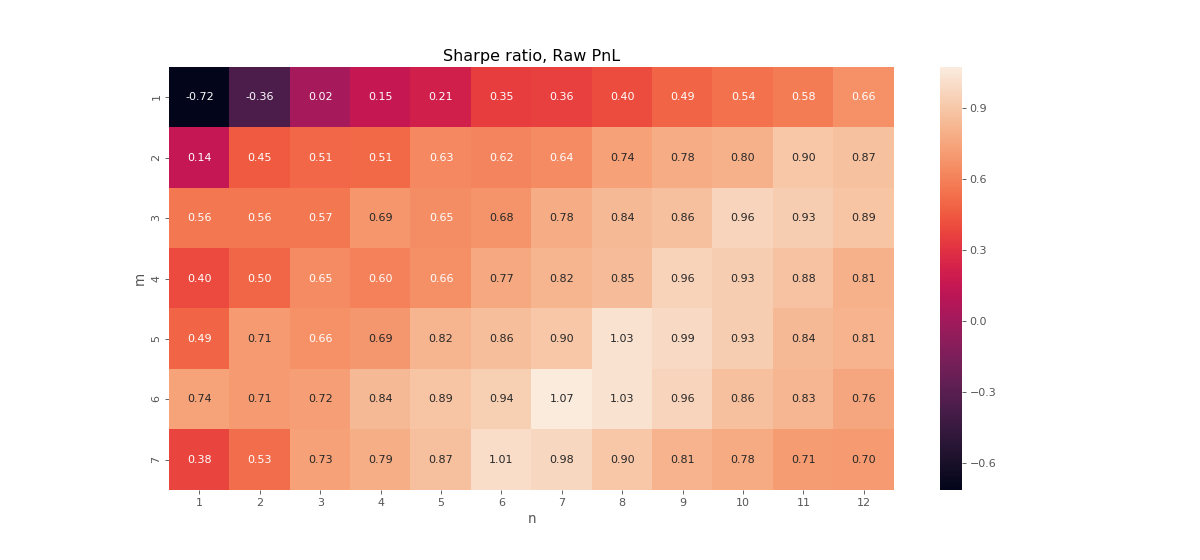
Top: Sharpe ratios of the cross-sectional stock momentum.
Stock returns are risk-managed, the universe is CRSP 1,000 most liquid stocks from 1963 to 2014.
Bottom: Sharpe ratio of the directional factor momentum.
Factors are beta-neutralised, risk-managed and computed on CRSP 1,000 most liquid stocks from 1963 to 2014.
We now move to computing the correlation between the two types of momentum. Results are reported in Figure 4. The heat map delivers a simple yet impressive result: the correlations are remarkably stable, around .5 across the board.
For different levels of and
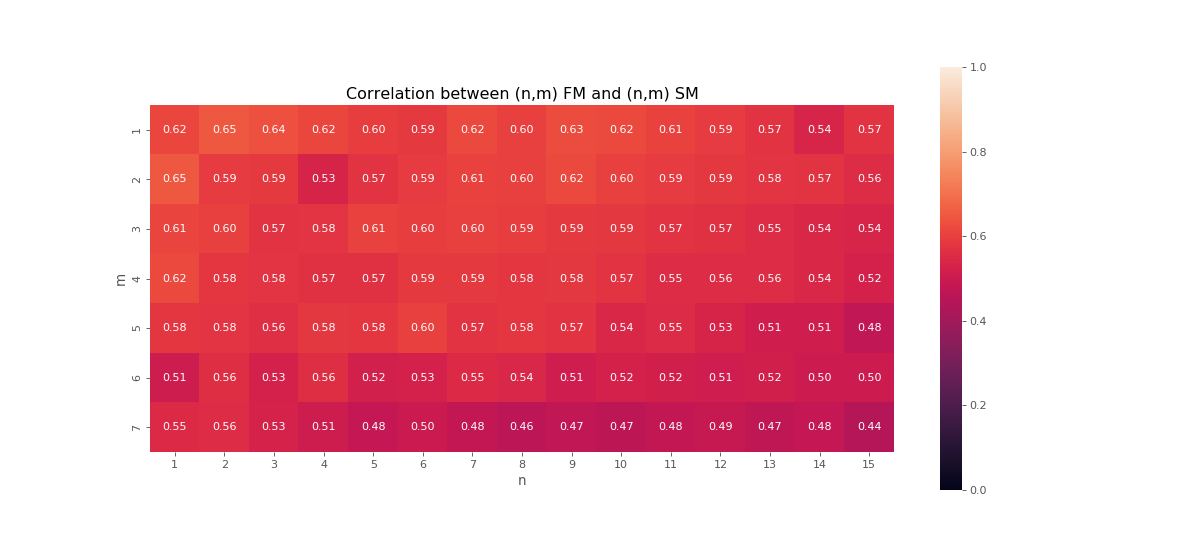
Stock returns are risk-managed, the universe is CRSP 1,000 most liquid stocks from 1963 to 2014.
The stability of the correlation across values of could be a priori surprising since we have just uncovered that for small values of and stocks and factor returns behave differently. So while it is natural to expect that the two strategies are correlated for , it is more surprising to find that they are positively correlated when their Sharpe ratios have opposite signs. The analysis of Section 4.1 provides an explanation for this. As shown in Equation (3) persistent factor exposure of stocks mechanically drives part of the correlation between both strategies: when factors perform well two periods in a row, stocks with positive beta do the same, while stocks with negative betas consistently sell off. Thus, this correlation is present, and does not depend on how well or badly the two momentums perform unconditionally.
4.3 Residual of factor momentum on stock momentum
We now proceed to analyze the residual of factor momentum on stock momentum. We have seen in Table 3 that factor momentum is not spanned by UMD (the residual has a Sharpe of 0.6). But now we want to incorporate what we have learnt by varying and , i.e. that the Sharpe of the two momentums vary quite differently as functions of lag and holding period. In addition, we also know from Section 3.3 that factor momentum is correlated with the menagerie factor, so we also want to include the latter in our spanning test.
Thus, in Figure 5, we show the Sharpe ratio of the residual of factor momentum after controlling for stock momentum, the menagerie factor and the market. All regressions use the entire sample (these are spanning tests, not hedging regressions). This residual is computed separately for each value of the lag and holding period .
After Taking out Stock Momentum, Menagerie and Market
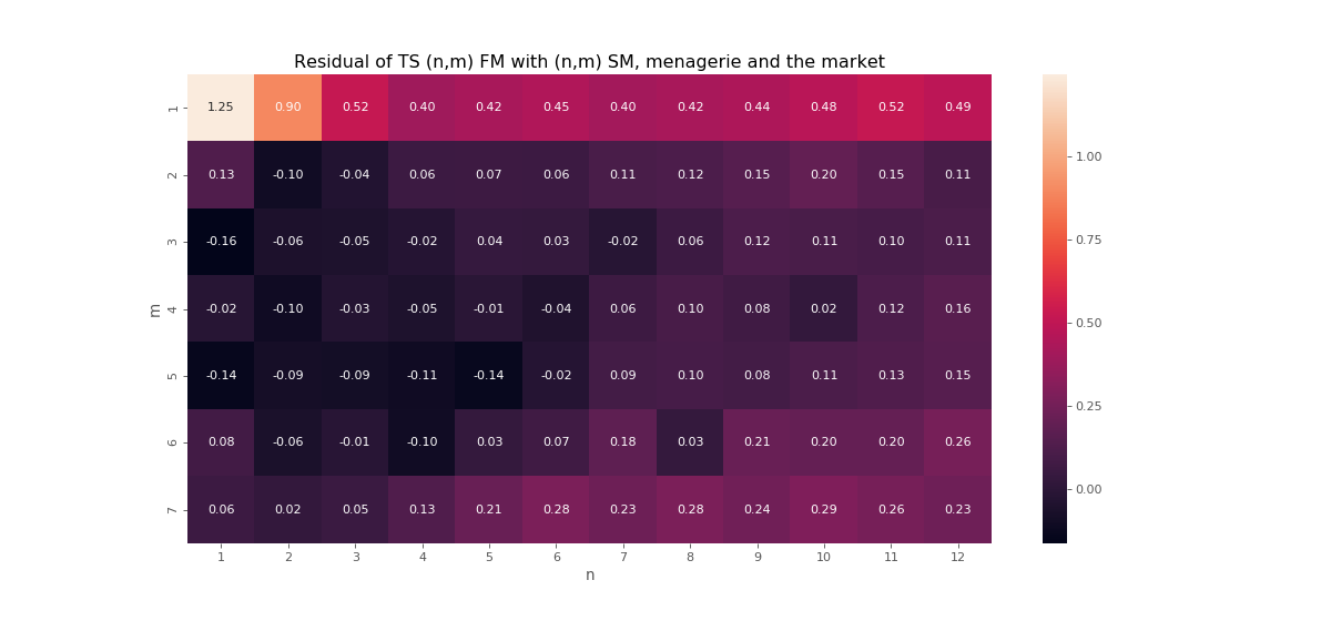
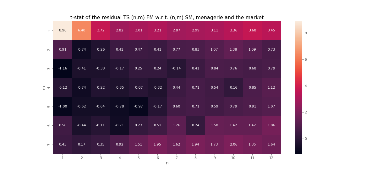
Stock returns are risk-managed, the universe is CRSP 1,000 most liquid stocks. Sample period from 1963 to 2014.
The heat map in Figure 5 suggests that that there is more to factor momentum than stock momentum, but only at lag , i.e. when we include the last month of returns. As soon as , the Sharpe ratios of residuals become insignificantly different from zero. This is consistent with the observation made in the previous section. The main difference between factor and stock momentum is that for stocks mean revert in the cross-section while factor returns persist. Our next section provides a framework that combines these effects.
Before we proceed, however, we would like to know whether stock and factor momentum are identical phenomena or whether factor momentum is just subsumed by stock momentum. In order to do this, we implement a spanning test opposite to the one proposed above, i.e. we regress stock momentum on factor momentum, menagerie and market for different values of and in order to single out the effect of lagging the signals. We report the results in Figure 6. For , due to mean-reversion, stock momentum is either negative or completely explained by the independent variables. For other values of , however, residual stock momentum is still significant for many cells in the heat map. This suggest that, while factor momentum is just stock momentum when , stock momentum is really something else for all values of .
After Taking out Factor Momentum, Menagerie and Market
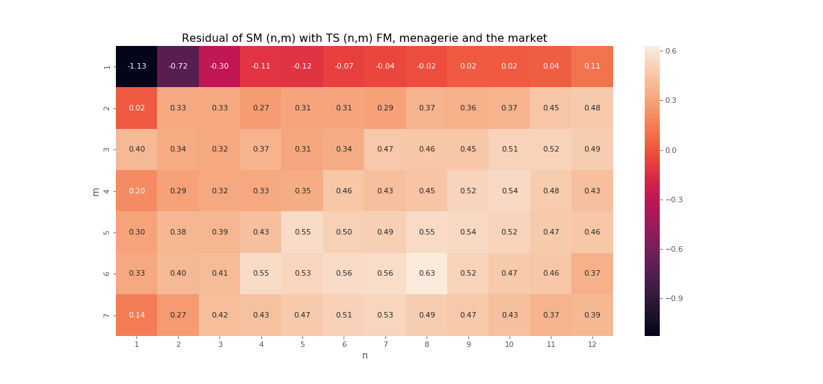
Stock returns are risk-managed, the universe is CRSP 1,000 most liquid stocks, from 1963 to 2014.
5 Framework
In this section, we will develop a heuristic model that encapsulates the three main stylized facts discussed in the previous Sections: (1) there is stock-level mean reversion at short lags and momentum at longer lags, (2) there is factor momentum at all lags and (3) there is a natural co-movement between the PNLs of stock and factor momentums at all horizons (short- and long-term).
5.1 Setup
We assume that there are different stocks and that there exists a factor strategy that attracts investors’ interest. This factor strategy is captured by a set of (normalized) positions on each of the stocks, which we assume fixed to simplify the exposition. We denote them by . We postulate that stock returns satisfy the equation below:
which can be derived from an equilibrium asset pricing model where three types of investors are present: Noise traders (who generate the mean-reverting noise ), factor investors (described below) and contrarian traders who have a limited ability to correct prices by leaning against the demand of the two other types of investors.
We assume the following behavior of factor investors. In line with the vast literature on the flow-performance relationship, we assume that these investors purchase additional amounts of the factor when it has performed well in the previous period. Past factor performance is given by the scalar and each stock is purchased in proportion , so that net factor purchases are proportional to the vector . The price impact of these imbalances is then assumed to be proportional to trading so that
This assumption is consistent with existing literature which documents that flow-induced trading has a predictable component (corresponding to pure scaling up or down of the fund’s portfolio in response to changes in AUMs) and that this component has a measurable price impact (Coval and Stafford (2007),Greenwood and Thesmar (2011), Lou (2012)).
We end up with the following equations of motion for stock returns:
which implies the following dynamics of factor returns
where we introduced which is a scalar. The law of motion of factor returns implies that there is autocorrelation of factor returns due to (performance-flow induced trading). is the unconditional expected return of the factor.
Finally, we assume that the stochastic term, , to be strongly mean-reverting. We assume its dynamics is governed by an MA1 process
where is a scalar and , where is the covariance matrix. Strong mean-reversion at fast time scales is an empirical fact for stocks. It is thus a short-memory process, while returns themselves, through positive feedback trading, have a longer memory.
5.2 Solving the Model & Results
Define . Stationarity implies that , which is an assumption we will be making. Then, returns can be shown to be described by the following equation:
where the terms in and represent the opposing forces of flow-induced trading () and noise trader demand ().
The autocovariance matrix of returns (of order ) is given by:
Using these formulas, it is straightforward to show our first result:
Proposition 1.
Factor momentum PNL
Let denote the expected factor variance. Then, the expected PNL of factor momentum is given by:
Thus, after controlling for mechanical exposure to factor investing (), there is factor momentum at all lags if and only if
In the second term of the above expressions, we rediscover that the expected PNL of factor momentum is positive even if there is no flow-induced trading (). This is a result we have seen previously: There is a mechanical relation between factor momentum and outright factor exposure.
But the interesting part of the above proposition is in the first term, which is the performance of factor momentum in excess of mechanical exposure to factor investing. This first term has the same sign at all horizons: If excess return of factor momentum is positive for , it will be positive at all horizons. This is consistent with what we find in the data (Table 3).
Let us now turn to stock momentum. Stock momentum is defined thourgh the trace of the autocovariance matrices
Proposition 2.
Stock momentum PNL
Write . The expected PNL of stock momentum at all horizons is given by:
Thus:
-
•
There is stock momentum at all horizons as long as
-
•
When starts dominating, there is mean-reversion for
This second proposition demonstrates that, whenever there is factor momentum (i.e. ), there is also stock momentum for all . In this sense factor momentum and stock momentum are indistinguishable: They occur for the same parameter values as soon as one excludes the most recent lag.
Another inference is that when the stock universe becomes large (keeping constant), becomes dominating and stock momentum becomes mean reversion for .
One last outcome of this analysis is that, stock momentum PNL () is a natural correlate of factor momentum if the values of or change. The expression below
is present both in stock momentum (for ) and in factor momentum. Variations in the aforementioned parameters tend to make the two strategies comove. This is because, in our model, stock momentum is subsumed in factor momentum (for ). An interesting extension of this model would be to introduce “idiosyncratic” stock momentum, for instance through assuming that follows an MA2 process with a positive loading on .
6 Conclusion
In this paper we have established that, for most implementations, factor momentum is fully accounted for by stock momentum and factor exposure. An important exception occurs at one month lag (and various holding periods). Including the last month of stock returns in the definition of stock momentum degrades its performance because stocks exhibit mean reversion at monthly time scale. This is not true for factor momentum, as factors returns are persistent at all time scales that we have studied. Consequently, “true” factor momentum only exists through the effect of the last month of returns. If we exclude it, factor momentum is pure stock momentum.
It is possible to reconcile these empirical observations with a simple model, which we provide and solve. This model predicts that both strategies (factor and stock momentum) are correlated between each other to a constant level, independently of the lag and the holding period, consistent with evidence that we find empirically.
References
- Abarbanell and Bushee (1998) Abarbanell, J. S. and B. J. Bushee (1998): “Abnormal Returns to a Fundamental Analysis Strategy,” The Accounting Review, 73, 19–45.
- Ali et al. (2003) Ali, A., L.-S. Hwang, and M. A. Trombley (2003): “Arbitrage risk and the book-to-market anomaly,” Journal of Financial Economics, 69, 355–373.
- Amihud (2002) Amihud, Y. (2002): “Illiquidity and stock returns: cross-section and time-series effects,” Journal of Financial Markets, 5, 31–56.
- Anderson and Garcia-Feijoo (2006) Anderson, C. W. and L. Garcia-Feijoo (2006): “Empirical Evidence on Capital Investment, Growth Options, and Security Returns,” The Journal of Finance, 61, 171–194.
- Ang et al. (2006) Ang, A., R. J. Hodrick, Y. Xing, and X. Zhang (2006): “The Cross-Section of Volatility and Expected Returns,” The Journal of Finance, 61, 259–299.
- Asness et al. (2000) Asness, C. S., R. B. Porter, and R. L. Stevens (2000): “Predicting Stock Returns Using Industry-Relative Firm Characteristics,” .
- Barbee et al. (1996) Barbee, W. C., S. Mukherji, and G. A. Raines (1996): “Do Sales–Price and Debt–Equity Explain Stock Returns Better than Book–Market and Firm Size?” Financial Analysts Journal, 52, 56–60.
- Basu (1977) Basu, S. (1977): “Investment Performance of Common Stocks in Relation to Their Price-Earnings Ratios: A Test of the Efficient Market Hypothesis,” The Journal of Finance, 32, 663–682.
- Bhandari (1988) Bhandari, L. C. (1988): “Debt/Equity Ratio and Expected Common Stock Returns: Empirical Evidence,” The Journal of Finance, 43, 507–528.
- Campbell and Shiller (1987) Campbell, J. and R. Shiller (1987): “Stock Prices, Earnings and Expected Dividends,” Journal of Finance.
- Chordia et al. (2001) Chordia, T., A. Subrahmanyam, and V. R. Anshuman (2001): “Trading activity and expected stock returns,” Journal of Financial Economics, 59, 3–32.
- Cohen et al. (2003) Cohen, Polk, and Vuolteenhao (2003): “The Value Spread,” Journal of Finance.
- Coval and Stafford (2007) Coval, J. and E. Stafford (2007): “Asset Fire Sales (and Purchases) on Equity Markets,” Journal of Financial Economics.
- Daniel and Titman (2006) Daniel, K. and S. Titman (2006): “Market Reactions to Tangible and Intangible Information,” The Journal of Finance, 61, 1605–1643.
- De Bondt and Thaler (1985) De Bondt, W. F. M. and R. Thaler (1985): “Does the Stock Market Overreact?” The Journal of Finance, 40, 793–805.
- Desai et al. (2004) Desai, H., S. Rajgopal, and M. Venkatachalam (2004): “Values-Glamour and Accruals Mispricing: One Anomaly or Two?” The Accounting Review, 79, 355–385.
- Ehsani and Linnainmaa (2019) Ehsani and Linnainmaa (2019): “Factor momentum and the momentum factor,” Tech. rep.
- Fama and French (1993) Fama, E. F. and K. R. French (1993): “Common risk factors in the returns on stocks and bonds,” Journal of Financial Economics, 33, 3–56.
- Francis et al. (2004) Francis, J., R. LaFond, P. M. Olsson, and K. Schipper (2004): “Costs of Equity and Earnings Attributes,” The Accounting Review, 79, 967–1010.
- Giglio et al. (2020) Giglio, Feng, and Xiu (2020): “Taming the Factor Zoo: a Test of New Factors,” Journal of Finance.
- Greenwood and Thesmar (2011) Greenwood, R. and D. Thesmar (2011): “Stock Price Fragility,” Journal of Financial Economics.
- Haddad et al. (2020) Haddad, Kozak, and Santosh (2020): “Factor Timing,” Review of Financial Studies.
- Hanson and Sunderam (2014) Hanson, S. and A. Sunderam (2014): “The Growth and Limits of Arbitrage: Evidence from Short Interest,” Review of Financial Studies.
- Harvey and Zhu (2016) Harvey, L. and Zhu (2016): “… and the cross-section of Expected Returns,” Review of Financial Studies.
- Haugen and Baker (1996) Haugen, R. A. and N. L. Baker (1996): “Commonality in the determinants of expected stock returns,” Journal of Financial Economics, 41, 401–439.
- Heston and Sadka (2008) Heston, S. L. and R. Sadka (2008): “Seasonality in the cross-section of stock returns,” Journal of Financial Economics, 87, 418–445.
- Holthausen and Larcker (1992) Holthausen, R. W. and D. F. Larcker (1992): “The prediction of stock returns using financial statement information,” Journal of Accounting and Economics, 15, 373–411.
- Hou and Moskowitz (2005) Hou, K. and T. J. Moskowitz (2005): “Market Frictions, Price Delay and the Cross-Section of Expected Returns,” The Review of Financial Studies, 18, 981–1020.
- Hou and Robinson (2006) Hou, K. and D. T. Robinson (2006): “Industry Concentration and Average Stock Returns,” The Journal of Finance, 61, 1927–1956.
- Hou and Zhang (2019) Hou, X. and . Zhang (2019): “Replicating anomalies,” Review of Financial Studies.
- Jegadeesh and Livnat (2006) Jegadeesh, N. and J. Livnat (2006): “Revenue surprises and stock returns,” Journal of Accounting and Economics, 41, 147–171.
- Jegadeesh and Titman (1993) Jegadeesh, N. and S. Titman (1993): “Returns to Buying Winners and Selling Losers: Implications for Stock Market Efficiency,” The Journal of Finance, 48, 65–91.
- Jiang et al. (2005) Jiang, G., C. M. C. Lee, and Y. Zhang (2005): “Information Uncertainty and Expected Returns,” Review of Accounting Studies, 10, 185–221.
- Lakonishok et al. (1994) Lakonishok, J., A. Shleifer, and R. W. Vishny (1994): “Contrarian investment, extrapolation, and risk,” The Journal of Finance, 49, 1541–1578.
- Lev and Nissim (2004) Lev, B. and D. Nissim (2004): “Taxable Income, Future Earnings, and Equity Values,” The Accounting Review, 79, 1039–1074.
- Liu (2006) Liu, W. (2006): “A liquidity-augmented capital asset pricing model,” Journal of Financial Economics, 82, 631–671.
- Lo and MacKinlay (1990) Lo, A. and C. MacKinlay (1990): “When are contrarian profits due to stock market overreaction?” The Review of Financial Studies, 3, 175–205.
- Lou (2012) Lou, D. (2012): “Flow-Based Explanation for Return Predictability,” Review of Financial Studies.
- Lyandres et al. (2008) Lyandres, E., L. Sun, and L. Zhang (2008): “The New Issues Puzzle: Testing the Investment-Based Explanation,” The Review of Financial Studies, 21, 2825–2855.
- McLean and Pontiff (2016) McLean and Pontiff (2016): “Does academic research destroy stock return predictability?” Journal of Finance.
- Moskowitz and Grinblatt (1999) Moskowitz, T. J. and M. Grinblatt (1999): “Do Industries Explain Momentum?” The Journal of Finance, 54, 1249–1290.
- Novy-Marx (2012) Novy-Marx, R. (2012): “Is Momentum Really Momentum?” Journal of Financial Economics, 103, 429–453.
- Ou and Penman (1989) Ou, J. A. and S. H. Penman (1989): “Financial Statement Analysis and the Prediction of Stock Returns,” Journal of Accounting and Economics, 11, 295–329.
- Pastor and Stambaugh (2003) Pastor, L. and R. F. Stambaugh (2003): “Liquidity Risk and Expected Stock Returns,” Journal of Political Economy, 111, 642–685.
- Piotroski (2000) Piotroski, J. D. (2000): “Value Investing: The Use of Historical Financial Statement Information to Separate Winners from Losers,” Journal of Accounting Research, 38, 1–41.
- Pontiff and Woodgate (2008) Pontiff, J. and A. Woodgate (2008): “Share Issuance and Cross-sectional Returns,” The Journal of Finance, 63, 921–945.
- Rendleman et al. (1982) Rendleman, R. J., C. P. Jones, and H. A. Latané (1982): “Empirical anomalies based on unexpected earnings and the importance of risk adjustments,” Journal of Financial Economics, 10, 269–287.
- Richardson et al. (2005) Richardson, S. A., R. G. Sloan, M. T. Soliman, and I. Tuna (2005): “Accrual reliability, earnings persistence and stock prices,” Journal of Accounting and Economics, 39, 437–485.
- Sloan (1996) Sloan, R. G. (1996): “Do Stock Prices Fully Reflect Information in Accruals and Cash Flows about Future Earnings?” The Accounting Review, 71, 289–315.
- Soliman (2008) Soliman, M. T. (2008): “The Use of DuPont Analysis by Market Participants,” The Accounting Review, 83, 823–853.
- Thomas and Zhang (2002) Thomas, J. K. and H. Zhang (2002): “Inventory Changes and Future Returns,” Review of Accounting Studies, 7, 163–187.
- Titman et al. (2004) Titman, S., J. K. C. Wei, and F. Xie (2004): “Capital Investments and Stock Returns,” Journal of Financial and Quantitative Analysis, 39, 677–700.
- Xing (2008) Xing, Y. (2008): “Interpreting the Value Effect Through the Q-Theory: An Empirical Investigation,” The Review of Financial Studies, 21, 1767–1795.
Appendix A List of Factors
| Factor | Reference article |
|---|---|
| Price earnings | Basu (1977) |
| Unexpected quarterly earnings | Rendleman et al. (1982) |
| Long term reversal | De Bondt and Thaler (1985) |
| Debt equity | Bhandari (1988) |
| Change in inventory-to-assets | Ou and Penman (1989) |
| Change in dividend per share | Ou and Penman (1989) |
| Change in capital expenditures-to-assets | Ou and Penman (1989) |
| Return on total assets | Ou and Penman (1989) |
| Debt repayment | Ou and Penman (1989) |
| Depreciation-to-PP&E | Holthausen and Larcker (1992) |
| Change in depreciation-to-PP&E | Holthausen and Larcker (1992) |
| Change in total assets | Holthausen and Larcker (1992) |
| Size | Fama and French (1993) |
| Book-to-market | Fama and French (1993) |
| Momentum | Jegadeesh and Titman (1993) |
| Sales growth | Lakonishok et al. (1994) |
| Cash flow-to-price | Lakonishok et al. (1994) |
| Working capital accruals | Sloan (1996) |
| Sales-to-price | Barbee et al. (1996) |
| Share turnover | Haugen and Baker (1996) |
| Cash flow-to-price variability | Haugen and Baker (1996) |
| Trading volume trend | Haugen and Baker (1996) |
| see next page |
| Factor | Reference article |
|---|---|
| Inventory | Abarbanell and Bushee (1998) |
| Gross margin | Abarbanell and Bushee (1998) |
| Capital expenditures | Abarbanell and Bushee (1998) |
| Industry momentum | Moskowitz and Grinblatt (1999) |
| F-score | Piotroski (2000) |
| Industry adjusted book-to-market | Asness et al. (2000) |
| Industry adjusted cash flow-to-price | Asness et al. (2000) |
| Industry adjusted size | Asness et al. (2000) |
| Industry adjusted momentum | Asness et al. (2000) |
| Industry adjusted long term reversal | Asness et al. (2000) |
| Industry adjusted short term reversal | Asness et al. (2000) |
| Dollar volume | Chordia et al. (2001) |
| Dollar volume coefficient of variation | Chordia et al. (2001) |
| Share turnover coefficient of variation | Chordia et al. (2001) |
| Change in inventory | Thomas and Zhang (2002) |
| Change in current assets | Thomas and Zhang (2002) |
| Depreciation | Thomas and Zhang (2002) |
| Change in accounts receivable | Thomas and Zhang (2002) |
| Other accruals | Thomas and Zhang (2002) |
| Illiquidity | Amihud (2002) |
| Liquidity | Pastor and Stambaugh (2003) |
| Idiosyncratic return volatility x book-to-market | Ali et al. (2003) |
| Price x book-to-market | Ali et al. (2003) |
| see next page |
| Factor | Reference article |
|---|---|
| Operating cash flow-to-price | Desai et al. (2004) |
| Abnormal corporate investment | Titman et al. (2004) |
| Accrual quality | Francis et al. (2004) |
| Earnings persistence | Francis et al. (2004) |
| Smoothness | Francis et al. (2004) |
| Value relevance | Francis et al. (2004) |
| Timeliness | Francis et al. (2004) |
| Tax income-to-book income | Lev and Nissim (2004) |
| Price delay | Hou and Moskowitz (2005) |
| Firm age | Jiang et al. (2005) |
| Duration | Jiang et al. (2005) |
| Change in current operating assets | Richardson et al. (2005) |
| Change in non-current operating liabilities | Richardson et al. (2005) |
| Growth in capital expenditures | Anderson and Garcia-Feijoo (2006) |
| Growth in capital expenditures (alternative) | Anderson and Garcia-Feijoo (2006) |
| Low volatility | Ang et al. (2006) |
| Low beta VIX | Ang et al. (2006) |
| Zero trading days | Liu (2006) |
| Composite issuance | Daniel and Titman (2006) |
| Intangible return | Daniel and Titman (2006) |
| Earnings surprises x revenue surprises | Jegadeesh and Livnat (2006) |
| Industry concentration | Hou and Robinson (2006) |
| Change in shares outstanding | Pontiff and Woodgate (2008) |
| Seasonality | Heston and Sadka (2008) |
| Investment | Lyandres et al. (2008) |
| Investment growth | Xing (2008) |
| Change in asset turnover | Soliman (2008) |
Appendix B Replication of Our Main Results Using Cross-Sectional Momentum
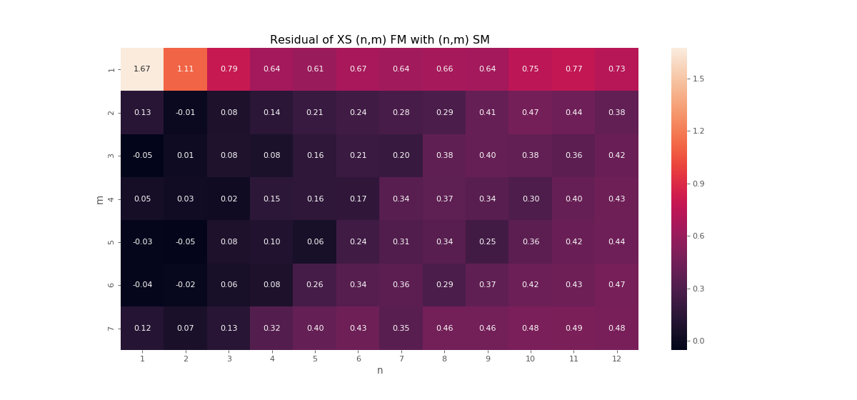
In this Appendix we replicate our main results from Figures 2, 3 and 4 using cross-sectional factor momentum instead of time-series factor momentum. The results are essentially identical. Figure B.1 shows the PNL of the cross-sectional factor momentum for various values of . Figure B.2 reports the correlation between stock and (cross-sectional) factor momentum. Figure B.3 shows the Sharpe ratio of the residual of factor momentum on stock momentum.
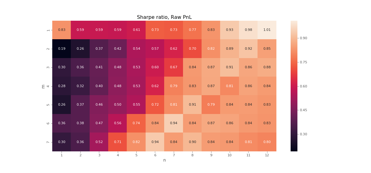
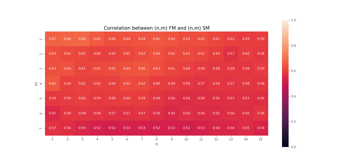
Stock returns are risk-managed and factors are beta-neutralised and risk-managed. The universe is CRSP 1,000 most liquid stocks (1963-2014).
Appendix C Proofs
C.1 Covariance between Factor and Stock Momentum
Assume the vector of stock returns follows a single factor structure
where we further assume that and are independent at all lags.
Then, the PNLs of (directional) factor momentum and stock momentum are given by the following two equations
where the lower bar stands for any combination of lag and holding period until date .
To calculate the covariance of these two PNLs, we start with the expectation of the product
We note and the conditional covariance and conditional expectation of . We assume homoskedastic, so that the conditional variance is constant, but we allow the conditional mean to vary over time (there can be factor momentum for instance). We use the fact that and are independent so that
Finally, we exploit the fact that cumulative returns have the same factor structure as one period returns, i.e. that . This leads to
Now, we need to compute the product of expectations
Combining the two expressions yields:
Noting that we obtain