Bayesian causal inference in probit graphical models

Abstract

We consider a binary response which is potentially affected by a set of continuous variables. Of special interest is the causal effect on the response due to an intervention on a specific variable. The latter can be meaningfully determined on the basis of observational data through suitable assumptions on the data generating mechanism. In particular we assume that the joint distribution obeys the conditional independencies (Markov properties) inherent in a Directed Acyclic Graph (DAG), and the DAG is given a causal interpretation through the notion of interventional distribution. We propose a DAG-probit model where the response is generated by discretization through a random threshold of a continuous latent variable and the latter, jointly with the remaining continuous variables, has a distribution belonging to a zero-mean Gaussian model whose covariance matrix is constrained to satisfy the Markov properties of the DAG. Our model leads to a natural definition of causal effect conditionally on a given DAG. Since the DAG which generates the observations is unknown, we present an efficient MCMC algorithm whose target is the posterior distribution on the space of DAGs, the Cholesky parameters of the concentration matrix, and the threshold linking the response to the latent. Our end result is a Bayesian Model Averaging estimate of the causal effect which incorporates parameter, as well as model, uncertainty. The methodology is assessed using simulation experiments and applied to a gene expression data set originating from breast cancer stem cells.

1 Introduction

We consider a system of random quantities, which includes a binary response as well as a collection of continuous variables, and address the problem of determining the causal effect on the response due to an intervention on a given variable. A causal question involves the data generating mechanism after an intervention is applied to the system, and must be carefully distinguished from traditional conditioning of probability theory (Pearl, 2009, Section 2.4). The gold standard for addressing causal questions is represented by randomized controlled experiments; the latter however are not always available because they may be unethical, infeasible, time consuming or expensive (Maathuis & Nandy, 2016). By contrast, observational data, that is observations produced without exogenous perturbations of the system, are widely available and often plentiful. The challenge is then to infer causal effects based on observational data alone. To achieve this goal, it is crucial to set up a a suitable conceptual framework which is able to address causal questions; in particular the notion of joint distribution for a collection of random variables can only address concepts linked to association, so much so that, by converse, “a causal concept is any relationship that cannot be defined from the distribution alone” (Pearl, 2009, Section 2).

A very useful framework to bridge the gap between the observational and the experimental domains is represented by the Directed Acyclic Graph (DAG), or its allied concept of Structural Equation Model (SEM); see Pearl (1995) and Pearl (2000). DAGs have been extensively used to construct statistical models embodying conditional independence relations (Lauritzen, 1996). Applications are numerous especially in genomics; see for instance Friedman (2004) and Friedman & Koller (2003). With observational data, conditional independence relations will drive inference on DAG and parameter space. On the other hand, the additional syntax and semantics of causal DAGs (Pearl, 2000) will be instrumental to define the notion of causal effect.

As in standard probit regression (Albert & Chib, 1993), we assume that the observable binary response is the result of a discretization of a continuous latent variable. Next, for a given DAG, we model all continuous random variables, along with the latent, as a multivariate Gaussian family satisfying the corresponding Markov property. We call the resulting setup a DAG-probit model, and provide a definition of causal effect on the response which is predicated on a given DAG through the notion of interventional distribution (Pearl, 2000). However the structure of the DAG is usually unknown, and this must be taken into account because different DAGs will typically induce distinct causal effects; see the review paper Maathuis & Nandy (2016) and Castelletti & Consonni (2020a) for a Bayesian approach.

In this work we extend the notion of interventional distribution and causal effect (Pearl, 2000; Maathuis et al., 2009) to DAG-probit models. Specifically, we propose a Bayesian method which jointly performs DAG-model determination as well as inference of causal effects in the presence of a binary response. From a computational viewpoint we introduce an MCMC scheme to sample from the joint posterior of models (DAGs) and model-dependent parameters (causal effects) which we implement through an efficient PAS algorithm (Godsill, 2012). The rest of the paper is organized as follows. In Section 2 we review DAG-Gaussian models and define the DAG-probit model. In Section 3 we present the structure of the interventional distribution in its general form, then specialize it to the Gaussian case, and finally extend the definition of causal effect to DAG-probit models. Section 4 presents our Bayesian methodology with particular emphasis on priors for model parameters. An MCMC algorithm for posterior inference on models, parameters and hence causal effects is presented in Section 5. We evaluate the proposed methodology through simulation studies in Section 6, and then apply it to a data set on gene expression measurements derived from breast cancer stem cells (Section 7). Finally a few points for discussion are presented in Section 8. Some theoretical results as well as additional simulation outputs are reported in the Supplementary material (Castelletti & Consonni, 2020b).

2 Model formulation

In this section we first provide some background material on Gaussian DAG-models with special emphasis on their parameterization (Section 2.1). Next we present our DAG-probit model (Section 2.2). Both sections deal with the likelihood, while choices of prior distributions are discussed in Section 4.

2.1 Gaussian DAG-models

Let $\mathcal{D}=(V,E)$ be a DAG, where $V=\{1,\dots,q\}$ is a set of vertices (or nodes) and $E\subseteq V\times V$ a set of edges whose elements are $(u,v)\equiv u\rightarrow v$, such that if $(u,v)\in E$ then $(v,u)\notin E$. In addition, $\mathcal{D}$ contains no cycles, that is paths of the form $u_{0}\rightarrow u_{1}\rightarrow\dots\rightarrow u_{k}$ where $u_{0}\equiv u_{k}$. For a given node $v$, if $u\rightarrow v\in E$ we say that $u$ is a parent of $v$ (conversely $v$ is a child of $u$). The parent set of $v$ in $\mathcal{D}$ is denoted by $\mathrm{pa}(v)$, the set of children by $\textnormal{ch}(v)$. Moreover, we denote by $\mathrm{fa}(v)=v\cup\mathrm{pa}(v)$ the family of $v$ in $\mathcal{D}$. For further theory and notation on DAGs we refer to Lauritzen (1996).

We consider a collection of random variables $(X_{1},\dots,X_{q})$ and assume that their joint probability density function $f(\bm{x})$ is Markov w.r.t. $\mathcal{D}$, so that it admits the following factorization

$$f(x_{1},\dots,x_{q})=\prod_{j=1}^{q}f(x_{j}\,|\,\bm{x}_{\mathrm{pa}(j)}).$$ (1)

In this section, as well as in Section 3, we reason conditionally on a given DAG $\mathcal{D}$ without an explicit conditioning in the notation we use. In Section 4 we will instead deal with model (DAG) uncertainty and will reinstate $\mathcal{D}$ in our notation.

If the joint distribution is Gaussian with mean equal to zero, we write

$$X_{1},\dots,X_{q}\,|\,\bm{\Omega}\sim\mathcal{N}_{q}(\bm{0},\bm{\Omega}^{-1}),\,\bm{\Omega}\in\mathcal{P}_{\mathcal{D}}$$ (2)

where $\bm{\Omega}=\bm{\Sigma}^{-1}$ is the precision matrix, and $\mathcal{P}_{\mathcal{D}}$ is the space of symmetric positive definite (s.p.d.) precision matrices Markov w.r.t. $\mathcal{D}$. For a Gaussian DAG-model factorization (1) becomes

$$f(x_{1},\dots,x_{q}\,|\,\bm{\Omega})=\prod_{j=1}^{q}d\,\mathcal{N}(x_{j}\,|\,\mu_{j}(\bm{x}_{\mathrm{pa}(j)}),\sigma_{j}^{2}),$$ (3)

where $d\,\mathcal{N}(\cdot\,|\,\mu,\sigma^{2})$ denotes the normal density having mean $\mu$ and variance $\sigma^{2}$. The assumption of normality guarantees that the model if faithful to the DAG, that is all and only those conditional independencies emboded in the joint distribution can be read-off from the graph using the Markov property; see also Spirtes et al. (2000).

Without loss of generality, we assume a parent ordering of the nodes which numerically labels the variables so that $i>j$ whenever $j$ is a child of $i$. A parent ordering always exists, although it is not unique in general. We also remark that a parent ordering is specific to any given DAG under consideration and may change if alternative DAGs are entertained. Importantly, it only represents a convenient device to specify a prior on the parameter space; see Section 4 where we also show that the choice of the parent ordering does not affect the prior assigned to model parameters.

Moreover, we declare node 1, which cannot have children, to be the (latent) outcome variable. Equation (3) can be also written as a structural equation model

$$\bm{L}^{\top}(X_{1},\dots,X_{q})^{\top}=\boldsymbol{\varepsilon},$$ (4)

where because of the assumed parent ordering $\bm{L}$ is a $(q,q)$ lower-triangular matrix of coefficients, $\bm{L}=\{\bm{L}_{ij},i\geq j\}$, such that $\bm{L}_{ij}\neq 0$ if and only if $i\rightarrow j$ and $\bm{L}_{ii}=1$. Moreover, $\boldsymbol{\varepsilon}$ is a $(q,1)$ vector of error terms, $\boldsymbol{\varepsilon}\sim\mathcal{N}_{q}(\boldsymbol{0},\bm{D})$, where $\bm{D}=\mathrm{diag}(\boldsymbol{\sigma}^{2})$ and $\boldsymbol{\sigma}^{2}$ is the $(q,1)$ vector of conditional variances whose $j$-th element is $\sigma^{2}_{j}=\mathbb{V}\!\mathrm{ar}(X_{j}\,|\,\bm{x}_{\mathrm{pa}(j)},\bm{\Omega})$. From (4) it follows that

$$\bm{\Omega}=\bm{L}\bm{D}^{-1}\bm{L}^{\top}.$$ (5)

We refer to Equation (5) as the modified Cholesky decomposition of $\bm{\Omega}$. Let now $\prec j\succ\,=\mathrm{pa}(j)$ and $\prec j\,]=\mathrm{pa}(j)\times j$. Representation (5) induces a re-parametrization of $\bm{\Omega}$ in terms of the Cholesky parameters $\left\{(\sigma_{j}^{2},\bm{L}_{\prec j\,]}),\,j=1,\dots,q\right\}$, where

$$\bm{L}_{\prec j\,]}=-\bm{\Sigma}_{\prec j\,\succ}\bm{\Sigma}_{\prec j\,]},\quad\sigma_{j}^{2}=\bm{\Sigma}_{jj\,|\,\mathrm{pa}(j)};$$

see also Cao et al. (2019). Accordingly, Equation (3) can be written as

$$f(x_{1},\dots,x_{q}\,|\,\bm{D},\bm{L})=\prod_{j=1}^{q}d\,\mathcal{N}(x_{j}\,|\,-\bm{L}_{\prec j\,]}^{\top}\bm{x}_{\mathrm{pa}(j)},\sigma_{j}^{2}),$$ (6)

with the understanding that the conditional expectation of $X_{j}$ in (6) is zero whenever ${\mathrm{pa}(j)}$ is the empty set.

2.2 DAG-probit models

We introduce in this section the general form of a DAG-probit model. We assume that the joint distribution of $(X_{1},X_{2},\dots,X_{q})$ is Gaussian and Markov w.r.t. $\mathcal{D}$ so that its density is as in (6). Recall that $X_{1}$ is latent and we are only allowed to observe the binary variable $Y\in\{0,1\}$. Specifically, for a given threshold $\theta_{0}\in(-\infty,+\infty)$, we assume that

$$Y=\begin{cases}\,\,1&\text{if $X_{1}\in[\,\theta_{0},+\infty)$},\\ \,\,0&\text{if $X_{1}\in(-\infty,\theta_{0})$}.\end{cases}$$ (7)

Combining (6) with (7), the joint density of $(Y,X_{1},\dots,X_{q})$ becomes

$$\begin{aligned} f(y,x_{1},\dots,x_{q}\,|\,\bm{D},\bm{L},\theta_{0})&=f(x_{1},\dots,x_{q}\,|\,\bm{D},\bm{L})\cdot\mathbbm{1}(\theta_{y-1}<x_{1}\leq\theta_{y})\\ &=\left\{\prod_{j=1}^{q}d\,\mathcal{N}(x_{j}\,|\,-\bm{L}_{\prec j\,]}^{\top}\bm{x}_{\mathrm{pa}(j)},\sigma_{j}^{2})\right\}\cdot\mathbbm{1}(\theta_{y-1}<x_{1}\leq\theta_{y}),\end{aligned}$$ (8)

where $\theta_{-1}=-\infty,\theta_{1}=+\infty$. Equation (8) defines a (Gaussian) DAG-probit model. A related expression appears in Guo et al. (2015) who model a multivariate distribution of ordered categorical variables through a collection of Gaussian random variables Markov with respect to an undirected graphical model. Now recall from (6) that the conditional distribution of the latent variable $X_{1}$ is $\mathcal{N}(-\bm{L}_{\prec 1\,]}^{\top}\bm{x}_{\mathrm{pa}(1)},\sigma_{1}^{2})$ and, as in standard probit regression, we set $\sigma_{1}^{2}=1$ for identifiability reasons.

Finally, by considering $n$ independent samples $(y_{i},x_{i,2},\dots,x_{i,q})$, $i=1,\dots,n$, from (8), the augmented likelihood can be written as

$$\begin{aligned} f(\bm{y},\bm{X}\,|\,\bm{D},\bm{L},\theta_{0})&=\prod_{i=1}^{n}f(x_{i,1},\dots,x_{i,q}\,|\,\bm{D},\bm{L})\cdot\mathbbm{1}(\theta_{y_{i}-1}<x_{i,1}\leq\theta_{y_{i}})\\ &=\prod_{j=1}^{q}d\,\mathcal{N}_{n}(\bm{X}_{j}\,|\,-\bm{X}_{\mathrm{pa}(j)}\bm{L}_{\prec j\,]},\sigma_{j}^{2}\bm{I}_{n})\cdot\left\{\prod_{i=1}^{n}\mathbbm{1}(\theta_{y_{i}-1}<x_{i,1}\leq\theta_{y_{i}})\right\},\end{aligned}$$ (9)

where $\bm{y}=(y_{1}\dots,y_{n})^{\top}$, $\bm{X}$ is the $(n,q)$ augmented data matrix, and $\bm{X}_{A}$ is the submatrix of $\bm{X}$ corresponding to the set $A$ of columns of $\bm{X}$.

3 Causal effects

Consider the joint density of the random vector $\left(X_{1},\dots,X_{q}\right)$ Markov w.r.t. a DAG which factorizes as in (1); the latter is referred to as the observational (or pre-intervention) distribution.

We now introduce the notion of intervention. A deterministic intervention on variable $X_{s}$, $s\in\{2,\dots,q\}$ is denoted by $\textnormal{do}(X_{s}=\tilde{x})$ and consists in setting $X_{s}$ to the value $\tilde{x}$. The post-intervention density of $(X_{1},\dots,X_{q})$ is then obtained using the truncated factorization

$$f(x_{1},\dots,x_{q}\,|\,\textnormal{do}(X_{s}=\tilde{x}))=\begin{cases}\prod\limits_{j=1,j\neq s}^{q}f(x_{j}\,|\,\bm{x}_{\mathrm{pa}(j)})|_{x_{s}=\tilde{x}}&\text{if $x_{s}=\tilde{x}$},\\ \quad\,0&\text{otherwise},\end{cases}$$ (10)

where, importantly, each term $f(x_{j}\,|\,\cdot)$ in (10) is the corresponding (pre-intervention) conditional distribution of Equation (1); see Pearl (2000). We emphasize that the post-intervention density $f(x_{1},\dots,x_{q}\,|\,\textnormal{do}(X_{s}=\tilde{x}))$ is conceptually distinct from the usual conditional density $f(x_{1},\dots,x_{q}\,|\,X_{s}=\tilde{x})$, which arises out of passive observation of $X_{s}=\tilde{x}$. An important feature of Equation (10) is that the data generating system is “stable” under exogenous interventions, in the sense that only the local component distribution $f(x_{s}\,|\,\bm{x}_{\mathrm{pa}(s)})$ is affected by the intervention and effectively reduces to a point mass on $\tilde{x}$. All the remaining terms are immune to the intervention and thus remain the same. The post-intervention distribution of the (latent) response $X_{1}$ is then obtained by integrating (10) w.r.t. $x_{2},\dots,x_{q}$ which simplifies to

$$f(x_{1}\,|\,\textnormal{do}(X_{s}=\tilde{x}))=\int f(x_{1}\,|\,\tilde{x},\bm{x}_{\mathrm{pa}(s)})f(\bm{x}_{\mathrm{pa}(s)})\,d\bm{x}_{\mathrm{pa}(s)};$$ (11)

see also Pearl (2000, Theorem 3.2.2).

We now move back to the Gaussian setting of Section 2.1, and assume that $(X_{1},X_{2},$ $\dots,X_{q})\,|\,\bm{\Sigma}\sim\mathcal{N}_{q}(\bm{0},\bm{\Sigma})$, where the covariance matrix $\bm{\Sigma}$ is Markov w.r.t. to the underlying DAG. The post-intervention distribution of $X_{1}$ can thus be written as

$$\begin{aligned} f(x_{1}\,|\,\textnormal{do}(X_{s}=\tilde{x}),\bm{\Sigma})=\int f(x_{1}\,|\,\tilde{x},\bm{x}_{\mathrm{pa}(s)},\bm{\Sigma})\cdot f(\bm{x}_{\mathrm{pa}(s)}\,|\,\bm{\Sigma})\,d\bm{x}_{\mathrm{pa}(s)}\\ =\int d\,\mathcal{N}(x_{1}\,|\,\gamma_{s}\tilde{x}+\bm{\gamma}^{\top}\bm{x}_{\mathrm{pa}(s)},\delta_{1}^{2})\cdot d\,\mathcal{N}(\bm{x}_{\mathrm{pa}(s)}\,|\,\bm{0},\bm{\Sigma}_{\mathrm{pa}(s),\mathrm{pa}(s)})\,d\bm{x}_{\mathrm{pa}(s)},\end{aligned}$$ (12)

where $\delta_{1}^{2}=\mathbb{V}\!\mathrm{ar}(X_{1}\,|\,X_{s}=\tilde{x},\bm{x}_{\mathrm{pa}(s)},\bm{\Sigma})$. The following Proposition gives the analytic form of the post-intervention distribution of $X_{1}$.

Proposition 3.1.

Let $(X_{1},X_{2},\dots,X_{q})\,|\,\bm{\Sigma}\sim\mathcal{N}_{q}(\bm{0},\bm{\Sigma})$ and consider the do operator $\textnormal{do}(X_{s}=\tilde{x})$, $s\in\{2,\dots,q\}$. Then the post-intervention distribution of $X_{1}$ is

$$f(x_{1}\,|\,\textnormal{do}(X_{s}=\tilde{x}),\bm{\Sigma})=d\,\mathcal{N}\left(x_{1}\,|\,\gamma_{s}\tilde{x},\frac{\delta_{1}^{2}}{1-(\bm{\gamma}^{\top}\bm{T}^{-1}\bm{\gamma})/\delta_{1}^{2}}\right),$$

where

$$\delta_{1}^{2} = \bm{\Sigma}_{1\,|\,\mathrm{fa}(s)},$$

$$(\gamma_{s},\bm{\gamma}^{\top})^{\top} = \bm{\Sigma}_{1,\mathrm{fa}(s)}\left(\bm{\Sigma}_{\mathrm{fa}(s),\mathrm{fa}(s)}\right)^{-1},$$

$$\bm{T} = \left(\bm{\Sigma}_{\mathrm{pa}(s),\mathrm{pa}(s)}\right)^{-1}+\frac{1}{\delta_{1}^{2}}\bm{\gamma}\bm{\gamma}^{\top},$$

with the understanding that node $s$ occupies the first position in the set $\mathrm{fa}(s)$.

Proof.

See Supplementary material (Castelletti & Consonni, 2020b). ∎

The previous reasoning considered the intervention distribution of the latent response variable $X_{1}$ following $\textnormal{do}(X_{s}=\tilde{x})$. Typically distribution (11) is summarized by its expected value $\mathbb{E}(X_{1}\,|\,\textnormal{do}(X_{s}=\tilde{x}))$. When $X_{s}$ is continuous, one can define the (total) causal effect as the derivative of $\mathbb{E}(X_{1}\,|\,\textnormal{do}(X_{s}={x}))$ w.r.t. $x$ evaluated at $\tilde{x}$: this is especially convenient when the expectation is linear, as in the Gaussian case (12), because the causal effect admits a simple interpretation: it corresponds to the “regression parameter” $\gamma_{s}$ associated to variable $X_{s}$ (Maathuis et al., 2009). Our interest however lies in the observable response variable $Y$, and therefore we aim to evaluate $\mathbb{E}(Y\,|\,\textnormal{do}(X_{s}=\tilde{x}),\bm{\Sigma},\theta_{0})$. We thus obtain

$$\begin{aligned} \mathbb{E}(Y\,|\,\textnormal{do}(X_{s}=\tilde{x}),\bm{\Sigma},\theta_{0})&=\textnormal{Pr}(Y=1\,|\,\textnormal{do}(X_{s}=\tilde{x}),\bm{\Sigma},\theta_{0})\\ &=\textnormal{Pr}(X_{1}\geq\theta_{0}\,|\,\textnormal{do}(X_{s}=\tilde{x}),\bm{\Sigma})\\ &=1-\Phi\left(\frac{\theta_{0}-\gamma_{s}\tilde{x}}{\tau_{1}}\right)\equiv\beta_{s}(\tilde{x},\bm{\Sigma},\theta_{0}),\end{aligned}$$ (13)

where $\Phi(\cdot)$ denotes the c.d.f. of a standard normal and $\tau^{2}_{1}=\delta_{1}^{2}/\left(1-(\bm{\gamma}^{\top}\bm{T}^{-1}\bm{\gamma})/\delta_{1}^{2}\right)$. One could then compute the partial derivative of $\mathbb{E}(Y\,|\,\textnormal{do}(X_{s}=\tilde{x}),\bm{\Sigma},\theta_{0})$ w.r.t $x$ evaluated at $\tilde{x}$, and obtain $\phi({\theta_{0}-\gamma_{s}\tilde{x}}/{\tau_{1}}){\gamma_{s}}/{\tau_{1}},$ where $\phi(\cdot)$ is the density function of a standard normal. This however would still depend on $\tilde{x}$. For this reason, and because (13) enjoys an intuitive interpretation being a probability, we will simply denote $\textnormal{Pr}(Y=1\,|\,\textnormal{do}(X_{s}=\tilde{x}),\bm{\Sigma},\theta_{0})$ at the causal effect on $Y$ due to an intervention $\textnormal{do}(X_{s}=\tilde{x})$. Finally, we remark that the causal effect of $\textnormal{do}(X_{s}=\tilde{x})$ on $Y$, besides being a function of the value $\tilde{x}$, depends on $\theta_{0}$ as well as on the covariance matrix $\bm{\Sigma}$, where the latter is constrained to be Markov w.r.t. the underlying DAG.

4 Bayesian inference

In this section we introduce priors for $(\bm{\Omega},\theta_{0},\mathcal{D})$, which we structure as $p(\bm{\Omega},\theta_{0},\mathcal{D})=p(\bm{\Omega}\,|\,\mathcal{D})p(\mathcal{D})p(\theta_{0})$. Further distributional results useful for our MCMC scheme of Section 5 are also presented. We briefly preview here the essential features.

To start with, consider $p(\bm{\Omega}\,|\,\mathcal{D})$, $\bm{\Omega}\in\mathcal{P}_{\mathcal{D}}$. We first proceed to the re-parameterization $\bm{\Omega}\mapsto(\bm{D},\bm{L})$ presented in Subsection 2.1, and specify a DAG-Wishart prior (Cao et al., 2019) on the Cholesky parameters $(\bm{D},\bm{L})$. We achieve this goal using a highly parsimonious elicitation procedure, which we detail in Section 4.1. For the unknown threshold $\theta_{0}\in(-\infty,+\infty)$, we assume a uniform prior, so that $p(\theta_{0})\propto 1$ (Section 4.3). Finally, a prior on DAG $\mathcal{D}$ is assigned through independent Bernoulli distributions on the elements of the skeleton of $\mathcal{D}$ (Section 4.2).

4.1 Prior on the Cholesky parameters

Consider first a DAG $\mathcal{D}=(V,E)$ which is complete, so that the precision matrix $\bm{\Omega}$ is unconstrained. A standard conjugate prior is the Wishart distribution, $\bm{\Omega}\sim\mathcal{W}_{q}(a,\bm{U})$ having expectation $a\bm{U}^{-1}$, where $a>q-1$ and $\bm{U}$ is a s.p.d. matrix. The induced prior on the Cholesky parameters consistent with the DAG parent ordering is such that the node parameters $(\sigma_{j}^{2},\bm{L}_{\prec j\,]})$, $j=1,\ldots,q$, are independent with distribution

$$\sigma_{j}^{2} \sim \textnormal{I-Ga}\left(\frac{a_{j}}{2}-\frac{|\mathrm{pa}(j)|}{2}-1,\frac{1}{2}\bm{U}_{jj|\prec j\succ}\right),$$

$$\bm{L}_{\prec j\,]}\,|\,\sigma_{j}^{2} \sim \mathcal{N}_{|\mathrm{pa}(j)|}\left(-\bm{U}_{\prec j\succ}^{-1}\bm{U}_{\prec j\,]},\sigma_{j}^{2}\bm{U}_{\prec j\succ}^{-1}\right),$$ (14)

where $|A|$ is the number of elements in the set $A$, $a_{j}=a+q-2j+3$; see Ben-David et al. (2015, Supplemental B). The symbol $\textnormal{I-Ga}(a,b)$ stands for an Inverse-Gamma distribution with shape $a>0$ and rate $b>0$ having expectation $b/(a-1)$ ($a>1$). In absence of substantive prior information, a standard choice for the hyperparameter $\bm{U}$, hereinafter adopted, is $\bm{U}=g\,\bm{I}_{q}$, where $g>0$ and $\bm{I}_{q}$ is the $(q,q)$ identity matrix. It is straightforward to show that (4.1) reduces to

$$\sigma_{j}^{2} \sim \textnormal{I-Ga}\left(\frac{a_{j}}{2}-\frac{|\mathrm{pa}(j)|}{2}-1,\frac{1}{2}\,g\right),$$

$$\bm{L}_{\prec j\,]}\,|\,\sigma_{j}^{2} \sim \mathcal{N}_{|\mathrm{pa}(j)|}\left(\bm{0},\frac{1}{g}\sigma_{j}^{2}\,\bm{I}_{|\mathrm{pa}(j)|}\right).$$ (15)

In addition, to guarantee the identifiability of the DAG-probit model, we fix $\sigma_{1}^{2}=1$, so that instead of $p(\sigma_{1}^{2},\bm{L}_{\prec 1\,]})$ we need only to consider $p(\bm{L}_{\prec 1\,]})$ with $\bm{L}_{\prec 1\,]}\sim\mathcal{N}_{|\mathrm{pa}(1)|}(\bm{0},$ $g^{-1}\,\bm{I}_{|\mathrm{pa}(1)|})$; see also Section 2.2. Recall that (4.1) applies only to a complete DAG $\mathcal{D}$.

Consider now the case in which $\mathcal{D}$ is not complete. The idea is to leverage (4.1) to construct a prior on $(\bm{D},\bm{L})$, the Cholesky parameters of $\bm{\Omega}\in\mathcal{P}_{\mathcal{D}}$, which is valid for any $\mathcal{D}$. To this end we follow the procedure of Geiger & Heckerman (2002). Specifically, let $\mathcal{D}$ be an arbitrary DAG and assume a parent ordering of its nodes. For each node $j\in\{1,\dots,q\}$, let $\big{\{}\sigma_{j}^{2},\bm{L}_{\prec j\,]}\big{\}}$ be the Cholesky parameters associated to node $j$, and identify a complete DAG $\mathcal{D}^{C(j)}$ such that $\mathrm{pa}_{\mathcal{D}^{C(j)}}(j^{\prime})=\mathrm{pa}_{\mathcal{D}}(j)$, where $j^{\prime}$ in $\mathcal{D}^{C}(j)$ corresponds to the same variable as $j$ in $\mathcal{D}$. Because of the parent ordering $j^{\prime}=q-|\mathrm{pa}_{\mathcal{D}}(j)|$ which is usually different from $j$. Let $\big{\{}\sigma_{j^{\prime}}^{2\,C(j)},\bm{L}_{\prec j^{\prime}\,]}^{C(j)}\big{\}}$ be the Cholesky parameters of node $j^{\prime}$ under the complete DAG $\mathcal{D}^{C(j)}$. We then assign to $\left\{\sigma_{j}^{2},\bm{L}_{\prec j\,]}\right\}$ the same prior of $\big{\{}\sigma_{j^{\prime}}^{2\,{C(j)}},\bm{L}_{\prec j^{\prime}\,]}^{C(j)}\big{\}}$ which can be gathered from Equation (4.1) in the complete DAG-Wishart version. In particular $\sigma_{j}^{2}\sim\textnormal{I-Ga}((a+|\mathrm{pa}_{\mathcal{D}}(j)|-q+3)/2-1,g/2)$ and $\bm{L}_{\prec j\,]}$ is distributed as a zero-mean multivariate normal with covariance matrix $g^{-1}\sigma_{j}^{2}\bm{I}_{|\mathrm{pa}_{\mathcal{D}}(j)|}$. Therefore both distributions only depend on the cardinality of $\mathrm{pa}_{\mathcal{D}}(j)$ which is the same across alternative parent orderings. Finally, by assuming independence among node-parameters $(\sigma_{j}^{2},\bm{L}_{\prec j\,]})$, we can write

$$p(\bm{D},\bm{L})=\prod_{j=1}^{q}p(\sigma_{j}^{2},\bm{L}_{\prec j\,]}),\quad(\bm{L},\bm{D})\in{\Theta}_{\mathcal{D}},$$ (16)

where ${\Theta}_{\mathcal{D}}$ is the image of the space $\mathcal{P}_{\mathcal{D}}$ under the mapping $\bm{\Omega}\mapsto(\bm{D},\bm{L})$.

4.2 Prior on DAG space

For a given DAG $\mathcal{D}$, let $\bm{A}^{\mathcal{D}}$ be the (symmetric) 0-1 adjacency matrix of the skeleton of $\mathcal{D}$ whose $(u,v)$ element is denoted by $\bm{A}^{\mathcal{D}}_{(u,v)}$. Conditionally on the edge inclusion probability $\pi$, we first assign a Bernoulli prior independently to each element $\bm{A}^{\mathcal{D}}_{(u,v)}$ belonging to the lower-triangular part, that is: $\bm{A}^{\mathcal{D}}_{(u,v)}\,|\,\pi\,\stackrel{{\scriptstyle iid}}{{\sim}}\,\textnormal{Ber}(\pi),u>v$. As a consequence we get

$$p(\bm{A}^{\mathcal{D}})=\pi^{|\bm{A}^{\mathcal{D}}|}(1-\pi)^{\frac{q(q-1)}{2}-|\bm{A}^{\mathcal{D}}|},$$ (17)

where $|\bm{A}^{\mathcal{D}}|$ denotes the number of edges in the skeleton, equivalently the number of entries equal to one in the lower-triangular part of $\bm{A}^{\mathcal{D}}$. Finally, we set $p(\mathcal{D})\propto p(\bm{A}^{\mathcal{D}})$, for $\mathcal{D}\in\mathcal{S}_{q}$, where $\mathcal{S}_{q}$ is the set of all DAGs on $q$ nodes.

4.3 Posterior distribution of $\theta_{0}$

As mentioned, in absence of substantive prior information, we assign a flat improper prior to the treshold $\theta_{0}\in(-\infty,\infty)$, $p(\theta_{0})\propto 1$. Accordingly, we need to prove that the posterior of $\theta_{0}$ is proper. The next proposition details under which conditions 2 is guaranteed.

Proposition 4.1.

Under the prior (4.1) for $(\bm{D},\bm{L})$, $p(\mathcal{D})$ as in Section 4.2 for DAG $\mathcal{D}$ and the improper prior $p(\theta_{0})\propto 1$ for $\theta_{0}$, the posterior of $\theta_{0}$ is proper provided the sample contains at least two observations with distinct values for $Y$, that is $y_{i}=1$, $y_{i^{\prime}}=0$ ($i\neq i^{\prime}$).

Proof.

See Supplementary material (Castelletti & Consonni, 2020b). ∎

Additionally, we prove in the Supplementary material that under the conditions of Proposition 4.1 the joint posterior of $(\bm{D},\bm{L},\mathcal{D},\theta_{0},\bm{X}_{1})$ is proper. Clearly, alternative priors for $\theta_{0}$ might have been used; yet the full conditional of $\theta_{0}$ would not be amenable to direct sampling. As a consequence, posterior inference on $\theta_{0}$ is performed through a Metropolis Hastings step inside our MCMC scheme; see Section 5 for details.

5 MCMC scheme

In this section we detail the MCMC scheme that we adopt to target the posterior distribution

$$p(\bm{D},\bm{L},\mathcal{D},\theta_{0},\bm{X}_{1}\,|\,\bm{y},\bm{X}_{-1})\propto f(\bm{y},\bm{X}\,|\,\bm{D},\bm{L},\mathcal{D},\theta_{0})\,p(\bm{D},\bm{L}\,|\,\mathcal{D})\,p(\mathcal{D}),$$ (18)

now emphasizing the dependence on DAG $\mathcal{D}$, where $\bm{X}_{-1}=(\bm{X}_{2},\ldots,\bm{X}_{q})$, and the term $p(\theta_{0})$ has been omitted because it is proportional to one.

5.1 Update of $(D,L,\mathcal{D})$

From (18) the full conditional distribution of $(\bm{D},\bm{L},\mathcal{D})$ is

$$p(\bm{D},\bm{L},\mathcal{D}\,|\,\bm{y},\bm{X},\theta_{0})\propto p(\bm{X}\,|\,\bm{D},\bm{L},\mathcal{D})p(\bm{D},\bm{L}\,|\,\mathcal{D})p(\mathcal{D})$$

using (9), where $\bm{X}=(\bm{X}_{1},\bm{X}_{2},\dots,\bm{X}_{q})$ is the $(n,q)$ augmented data matrix.

To sample from $p(\bm{D},\bm{L},\mathcal{D}\,|\,\bm{X})$ we adopt a reversible jump MCMC algorithm which takes into account the partial analytic structure (PAS, Godsill 2012) of the DAG-Wishart distribution to sample DAG $\mathcal{D}$ and the Cholesky parameters $(\bm{D},\bm{L})$ from their full conditional. A similar approach was implemented in Wang & Li (2012) for Gaussian undirected graphical models using G-Wishart priors. Details about the PAS algorithm and its implementation in our DAG setting are reported in the Supplementary material (Castelletti & Consonni, 2020b).

Specifically, at each iteration of the MCMC scheme, we first propose a new DAG $\mathcal{D}^{\prime}$ from a suitable proposal distribution $q(\mathcal{D}^{\prime}\,|\,\mathcal{D})$; see again our Supplementary material. In particular, it is shown that when proposing a DAG $\mathcal{D}^{\prime}$ which differs from the current graph $\mathcal{D}$ by one edge $(h,j)$, the acceptance probability for $\mathcal{D}^{\prime}$ is given by

$$\alpha_{\mathcal{D}^{\prime}}=\min\left\{1,\frac{m(\bm{X}_{j}\,|\,\bm{X}_{\mathrm{pa}_{\mathcal{D}^{\prime}}(j)},\mathcal{D}^{\prime})}{m(\bm{X}_{j}\,|\,\bm{X}_{\mathrm{pa}_{\mathcal{D}}(j)},\mathcal{D})}\cdot\frac{p(\mathcal{D}^{\prime})}{p(\mathcal{D})}\cdot\frac{q(\mathcal{D}\,|\,\mathcal{D}^{\prime})}{q(\mathcal{D}^{\prime}\,|\,\mathcal{D})}\right\}$$ (19)

where, for $j\in\{2,\dots,q\}$,

$$m(\bm{X}_{j}\,|\,\bm{X}_{\mathrm{pa}_{\mathcal{D}}(j)},\mathcal{D})=(2\pi)^{-\frac{n}{2}}\frac{\big{|}\bm{T}_{j}\big{|}^{1/2}}{\big{|}\bar{\bm{T}}_{j}\big{|}^{1/2}}\cdot\frac{\Gamma\left(a_{j}^{*}+\frac{n}{2}\right)}{\Gamma\left(a_{j}^{*}\right)}\left[\frac{1}{2}g\right]^{a_{j}^{*}}\left[\frac{1}{2}\big{(}g+\bm{X}_{j}^{\top}\bm{X}_{j}-\hat{\bm{L}}_{j}^{\top}\bar{\bm{T}}_{j}\hat{\bm{L}}_{j}\big{)}\right]^{-(a_{j}^{*}+n/2)}$$ (20)

with

$$\bm{T}_{j} = g\bm{I}_{|\mathrm{pa}_{\mathcal{D}}(j)|}$$

$$\bar{\bm{T}}_{j} = g\bm{I}_{|\mathrm{pa}_{\mathcal{D}}(j)|}+\bm{X}_{\mathrm{pa}_{\mathcal{D}}(j)}^{\top}\bm{X}_{\mathrm{pa}_{\mathcal{D}}(j)}$$

$$\hat{\bm{L}}_{j} = \big{(}g\bm{I}_{|\mathrm{pa}_{\mathcal{D}}(j)|}+\bm{X}_{\mathrm{pa}_{\mathcal{D}}(j)}^{\top}\bm{X}_{\mathrm{pa}_{\mathcal{D}}(j)}\big{)}^{-1}\bm{X}_{\mathrm{pa}_{\mathcal{D}}(j)}^{\top}\bm{X}_{j},$$

$a_{j}^{*}=\frac{a_{j}}{2}-\frac{|\mathrm{pa}_{\mathcal{D}}(j)|}{2}-1$ and $\bm{X}_{\mathrm{pa}_{\mathcal{D}}(j)}$ denotes the $(n,|\mathrm{pa}_{\mathcal{D}}(j)|)$ sub-matrix of $\bm{X}$ whose columns belong to the set $\mathrm{pa}_{\mathcal{D}}(j)$. For $j=1$, because we fixed $\sigma_{1}^{2}=1$, we have instead

$$m(\bm{X}_{1}\,|\,\bm{X}_{\mathrm{pa}_{\mathcal{D}}(1)},\mathcal{D})=(2\pi)^{-\frac{n}{2}}\frac{\big{|}\bm{T}_{1}\big{|}^{1/2}}{\big{|}\bar{\bm{T}}_{1}\big{|}^{1/2}}\cdot\exp\left\{-\frac{1}{2}\big{(}\bm{X}_{1}^{\top}\bm{X}_{1}+\hat{\bm{L}}_{1}^{\top}\bar{\bm{T}}_{1}\hat{\bm{L}}_{1}\big{)}\right\},$$ (21)

with $\bm{T}_{1},\bar{\bm{T}}_{1},\hat{\bm{L}}_{1}$ defined in analogy with the expressions appearing after (20); see the Supplementary material (Castelletti & Consonni, 2020b) for details. Moreover, given DAG $\mathcal{D}$ and $\bm{X}_{1}$, the full conditional of $(\bm{D},\bm{L})$ reduces to the augmented posterior $p(\bm{D},\bm{L}\,|\,\bm{X})$, which is conditional on the actual data $(\bm{X}_{2},\ldots,\bm{X}_{q})$ as well as the latent values $\bm{X}_{1}$ and can be easily sampled from. Specifically, since

$$f(\bm{X}\,|\,\bm{D},\bm{L})=\prod_{j=1}^{q}d\,\mathcal{N}_{n}(\bm{X}_{j}\,|\,-\bm{X}_{\mathrm{pa}_{\mathcal{D}}(j)}\bm{L}_{\prec j\,]},\sigma_{j}^{2}\bm{I}_{n})$$ (22)

and because of (16) and conjugacy of the Normal-Inverse-Gamma prior in (4.1) with the Normal density, the posterior distribution of the Cholesky parameters given $\bm{X}$ is, for $j=2,\dots,q$,

$$\sigma_{j}^{2}\,|\,\bm{X} \sim \textnormal{I-Ga}\left(a_{j}^{*}+\frac{n}{2},\frac{1}{2}\big{(}g+\bm{X}_{j}^{\top}\bm{X}_{j}-\hat{\bm{L}}_{j}^{\top}\bar{\bm{T}}_{j}\hat{\bm{L}}_{j}\big{)}\right),$$

$$\bm{L}_{\prec j\,]}\,|\,\sigma_{j}^{2},\bm{X} \sim \mathcal{N}_{|\mathrm{pa}_{\mathcal{D}}(j)|}\big{(}-\hat{\bm{L}}_{j},\sigma_{j}^{2}\bar{\bm{T}}_{j}^{-1}\big{)}.$$ (23)

Moreover, for node $1$ where $\sigma_{1}^{2}=1$, we have

$$\bm{L}_{\prec 1\,]}\,|\,\bm{X} \sim \mathcal{N}_{|\mathrm{pa}_{\mathcal{D}}(1)|}\big{(}-\hat{\bm{L}}_{1},\bar{\bm{T}}_{1}^{-1}\big{)}.$$ (24)

5.2 Update of $X_{1}$ and $\theta_{0}$

Updating of $\bm{X}_{1}=(x_{1,1},\dots,x_{n,1})^{\top}$ can be performed by direct sampling from the full conditional distribution of each latent observation $x_{i,1}$,

$$f(x_{i,1}\,|\,y_{i},x_{i,2},\dots,x_{i,q},\bm{D},\bm{L},\mathcal{D},\theta_{0})\propto f(x_{i,1}\,|\,\bm{x}_{i,\mathrm{pa}_{\mathcal{D}}(1)},\bm{L}_{\prec j\,]})\cdot\mathbbm{1}(\theta_{y_{i}-1}<x_{i,1}\leq\theta_{y_{i}}),$$

which corresponds to a $\mathcal{N}(-\bm{L}_{\prec 1\,]}^{\top}\bm{x}_{i,\mathrm{pa}_{\mathcal{D}}(1)},1)$ truncated at the interval $(\theta_{y_{i}-1},\theta_{y_{i}}]$.

Finally, the cut-off $\theta_{0}$ is updated through a Metropolis Hastings step where, given the current value $\theta_{0}$, a candidate value $g_{0}$ is proposed from $q(g_{0}\,|\,\theta_{0})=d\,\mathcal{N}(g_{0}\,|\,\theta_{0},\sigma_{0}^{2})$. We then set $\theta_{0}=g_{0}$ with probability

$$\alpha_{\theta}=\min\left\{1;r_{\theta}\right\},$$ (25)

where

$$r_{\theta}\,=\,\frac{\prod\limits_{i=1}^{n}\left[\Phi\big{(}g_{y_{i}}\,|\,-\bm{L}_{\prec 1\,]}^{\top}\bm{x}_{i,\mathrm{pa}_{\mathcal{D}}(1)},1\big{)}-\Phi\big{(}g_{y_{i}-1}\,|\,-\bm{L}_{\prec 1\,]}^{\top}\bm{x}_{i,\mathrm{pa}_{\mathcal{D}}(1)},1\big{)}\right]}{\prod\limits_{i=1}^{n}\left[\Phi\big{(}\theta_{y_{i}}\,|\,-\bm{L}_{\prec 1\,]}^{\top}\bm{x}_{i,\mathrm{pa}_{\mathcal{D}}(1)},1\big{)}-\Phi\big{(}\theta_{y_{i}-1}\,|\,-\bm{L}_{\prec 1\,]}^{\top}\bm{x}_{i,\mathrm{pa}_{\mathcal{D}}(1)},1\big{)}\right]}\cdot\frac{d\,\mathcal{N}\left(\theta_{0}\,|\,g_{0},\sigma_{0}^{2}\right)}{d\,\mathcal{N}\left(g_{0}\,|\,\theta_{0},\sigma_{0}^{2}\right)},$$

and $g_{-1}=\infty,g_{1}=+\infty$.

5.3 Algorithm

Algorithm 1 summarizes our MCMC scheme. The output is a collection of DAGs $\big{\{}\mathcal{D}^{(t)}\big{\}}_{t=1}^{T}$ and Cholesky parameters $\big{\{}\big{(}\bm{D}^{\mathcal{D}^{(t)}},\bm{L}^{\mathcal{D}^{(t)}}\big{)}\big{\}}_{t=1}^{T}$ approximatively sampled from the target distribution (18). In particular we can compute posterior summaries of interest such as the posterior probabilities of edge inclusion, namely

$$\hat{p}_{u\rightarrow v}(\bm{y},\bm{X}_{2},\dots,\bm{X}_{q})\equiv\hat{p}_{u\rightarrow v}=\frac{1}{T}\sum_{t=1}^{T}\mathbbm{1}_{u\rightarrow v}\big{\{}\mathcal{D}^{(t)}\big{\}},$$ (26)

where $\mathbbm{1}_{u\rightarrow v}\big{\{}\mathcal{D}^{(t)}\big{\}}$ takes value 1 if and only if $\mathcal{D}^{(t)}$ contains the edge $u\rightarrow v$. Moreover, we can reconstruct the covariance matrices $\big{\{}\bm{\Sigma}^{\mathcal{D}^{(t)}}\big{\}}_{t=1}^{T}$ using (5). The latter can be subsequently retrieved to obtain for selected $s\in\{2,\dots,q\}$ and intervention value $\tilde{x}$ the collection of causal effects $\big{\{}\beta_{s}^{(t)}(\tilde{x})\big{\}}_{t=1}^{T}$ defined in (13), where we set $\beta_{s}^{(t)}(\tilde{x})\equiv\beta_{s}\big{(}\tilde{x},\bm{\Sigma}^{\mathcal{D}^{(t)}},\theta_{0}^{(t)}\big{)}$. An overall summary of the causal effect of $\textnormal{do}(X_{s}=\tilde{x})$ on $Y$ can be computed as

$$\hat{\beta}_{s}^{BMA}(\tilde{x})=\frac{1}{T}\sum_{t=1}^{T}\beta_{s}^{(t)}(\tilde{x}),$$ (27)

which corresponds to a Bayesian Model Averaging (BMA) estimate where posterior (DAG) model probabilities are approximated through the MCMC frequencies of visits; see García-Donato & Martínez-Beneito (2013) for a discussion of the merits of frequency based estimators in large model spaces.

Input: A dataset $(\bm{y},\bm{X}_{2},\dots,\bm{X}_{q})$

Output: $T$ samples from the posterior (18)

1 Initialize $\mathcal{D}^{(0)}$, e.g. the empty DAG, the cut-offs $\theta_{-1}^{(0)}=-\infty,\theta_{0}^{(0)}=0,\theta_{1}^{(0)}=+\infty$ and the latent variables $\bm{x}_{1}^{(0)}$, e.g. $x_{i,1}^{(0)}\stackrel{{\scriptstyle ind}}{{\sim}}\mathcal{N}(0,1)$ truncated at $(\theta^{(0)}_{y_{i}-1},\theta^{(0)}_{y_{i}}]$;

2 for $t=1,\dots,T$ do

3       Sample $\mathcal{D}^{\prime}$ from $q(\mathcal{D}^{\prime}\,|\,\mathcal{D}^{(t-1)})$ and set $\mathcal{D}^{(t)}=\mathcal{D}^{\prime}$ with probability $\alpha_{\mathcal{D}}$ (19), otherwise $\mathcal{D}^{(t)}=\mathcal{D}^{(t-1)}$;

4       Sample $\big{(}\bm{D}^{\mathcal{D}^{(t)}},\bm{L}^{\mathcal{D}^{(t)}}\big{)}$ from its augmented posterior distribution (5.1);

5       For $i=1,\dots,n$, independently sample $x_{i,1}$ from $\mathcal{N}\big{(}-\bm{L}_{\prec 1\,]}^{\mathcal{D}^{(t)}\top}\bm{x}_{i,\mathrm{pa}_{\mathcal{D}^{(t)}}(1)},1\big{)}$ truncated at $(\theta_{y_{i}-1}^{(t)},\theta_{y_{i}}^{(t)}]$;

6       Propose a cut-off $g_{0}$ from $q(g_{0}\,|\,\theta_{0}^{(t)})$ and set $\theta_{0}^{(t)}=g_{0}$ with probability $\alpha_{\theta}$ (25), otherwise $\theta_{0}^{(t)}=\theta_{0}^{(t-1)}$; set $\theta_{-1}^{(t)}=-\infty,\theta_{1}^{(t)}=+\infty$.

7 end for

8

Algorithm 1 MCMC scheme to sample from (18)

6 Simulations

In this section we evaluate the performance of our method through simulation studies. Specifically, for each combination of number of nodes $q\in\{20,40\}$ and sample size $n\in\{100,200,500\}$, which we call simulation scenario, we generate $40$ DAGs using a probability of edge inclusion equal to $p=3/(2q-2)$ to induce sparsity; see Peters & Bühlmann (2014). For each DAG $\mathcal{D}$ we then proceed as follows. We identify a parent ordering and fix $\bm{D}^{\mathcal{D}}=\bm{I}_{q}$ and then randomly sample the entries of $\bm{L}^{\mathcal{D}}$ in the interval $[-2,-1]\cup[1,2]$; next we generate a dataset consisting of $n$ i.i.d. $q$-dimensional observations from the structural equation model (4) which also includes the $(n,1)$ vector of latent observations; we finally fix the threshold $\theta_{0}=0$ and obtain the 0-1 vector of responses $\bm{y}=(y_{1},\dots,y_{n})^{\top}$ as in (7).

We apply Algorithm 1 to approximate the target distribution in (18) by setting the number of MCMC iterations $T=25000$ for $q=20$, and $T=50000$ for $q=40$. We also set $g=1/n$ and $a=q+1$ in the prior on the Cholesky parameters of $\bm{\Omega}$ (4.1) and $\sigma_{0}^{2}=0.25$ in the proposal density for the cut-off $\theta_{0}$.

We begin by evaluating the global performance of our method in learning the graph structure. To this end, we first estimate the posterior probabilities of edge inclusion by computing $\hat{p}_{u\rightarrow v}(\cdot)$ in (26) for each pair of distinct nodes $u,v$. Next, we consider a threshold for edge inclusion $k\in[0,1]$ and for a given $k$ construct a DAG estimate by including those edges $(u,v)$ whose posterior probability exceeds $k$. The resulting graph is compared with the true DAG through the sensitivity (SEN) and specificity (SPE) indexes, respectively defined as

$$SEN=\frac{TP}{TP+FN},\quad SPE=\frac{TN}{TN+FP},$$

where $TP,TN,FP,FN$ are the numbers of true positives, true negatives, false positives and false negatives respectively. The two indexes are used to construct a receiver operating characteristic (ROC) curve. Specifically, for each scenario defined by $q$ and $n$, we present a ROC curve constructed as follows. For each threshold $k$, we compute $SEN$ and $(1-SPE)$ under each of the 40 DAGs used in the simulation. The point whose coordinates are the mean of each of the two measures corresponds to one dot in Figure 1. The collection of dots connected by lines represents an average ROC curve. We proceed similarly to compute the 5th and 95th percentile and obtain the grey band.

To better appreciate Figure 1, we also compute, for each simulation scenario $(q,n)$, the area under the (average) ROC curve (AUC) whose values are reported in Table 1. They are close or above 94% under the three sample sizes considered when $q=20$. When $q=40$ AUC exceeds 90% for $n=100$ and rises to over 97% for $n=500$.

$\quad\quad n=100$	$\quad\quad n=200$	$\quad\quad n=500$

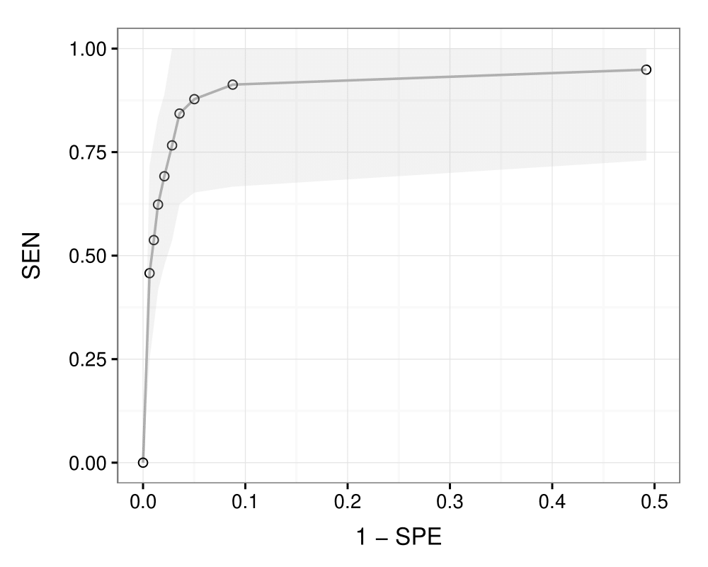
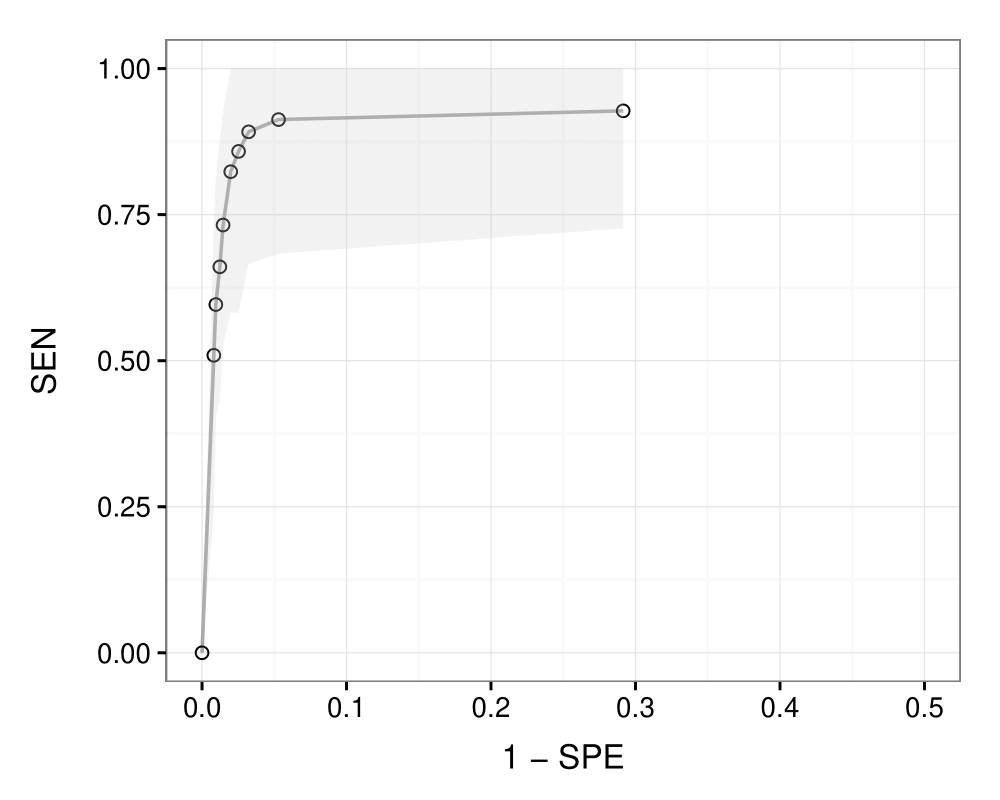
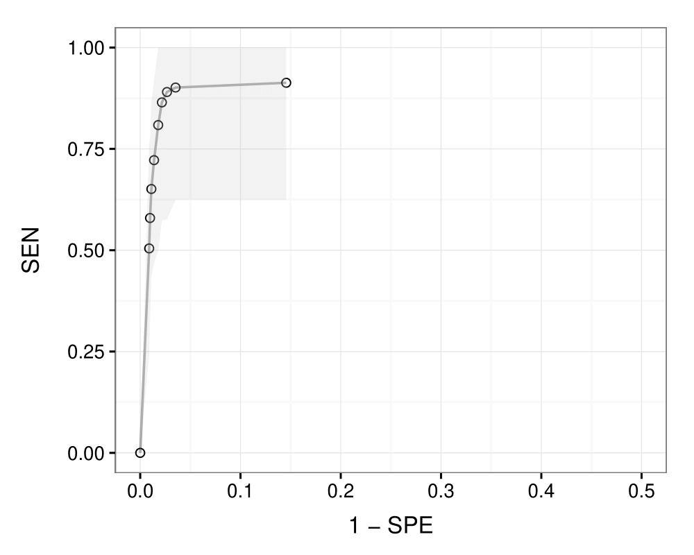
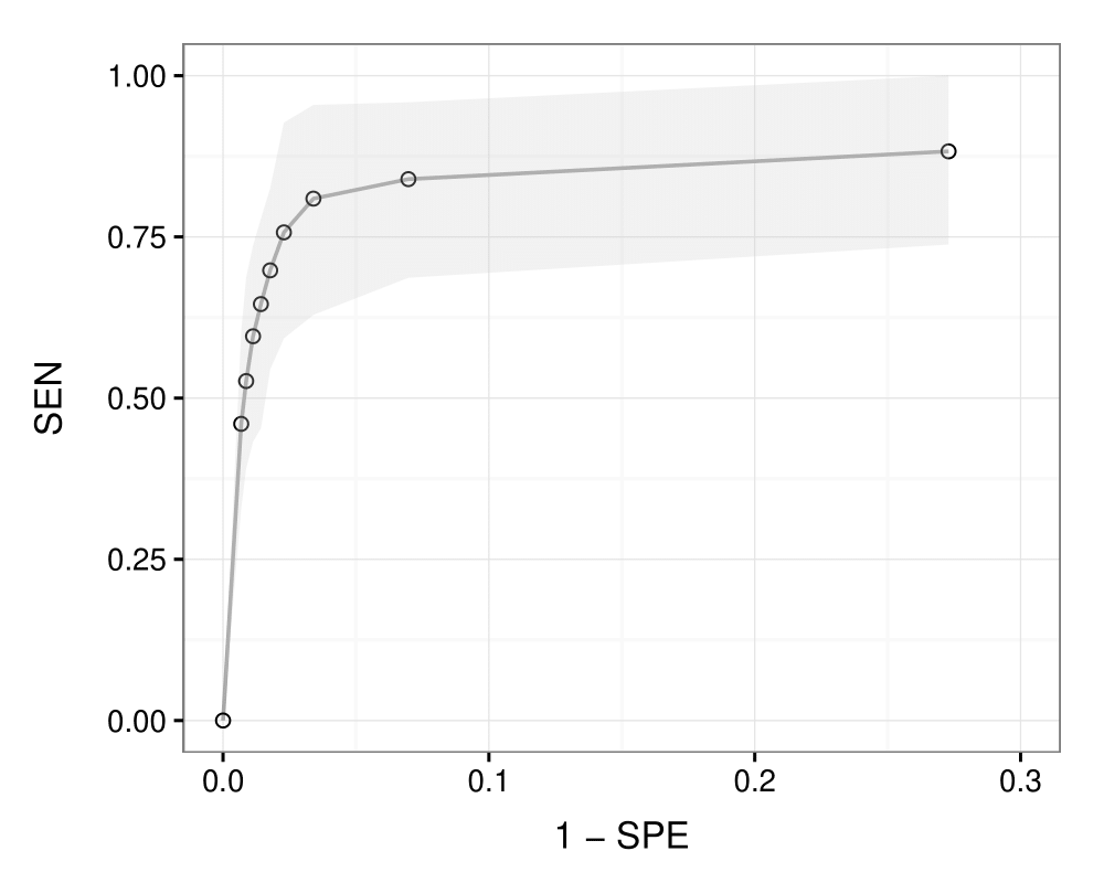
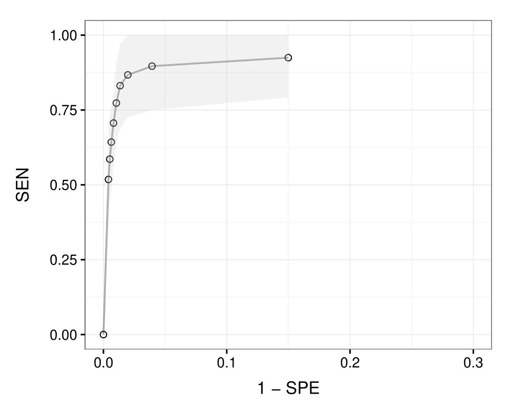
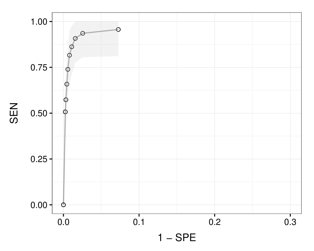
Figure 1: Simulations. Receiver operating characteristic (ROC) curve obtained under varying thresholds for the posterior probabilities of edge inclusion for each combination of number of nodes $q=\{20,40\}$ (first and second row respectively) and sample size $n\in\{100,200,500\}$. Dots and connecting line describe the (average over the 40 simulated DAGs) ROC curve, while the grey area represents the 5th-95th percentile band.

	$n=100$	$n=200$	$n=500$
$q=20$	93.89	94.19	95.12
$q=40$	90.94	94.91	97.19

Table 1: Simulations. Area under the curve (percentage values) computed from the average ROC curves in Figure 1 for number of nodes $q\in\{20,40\}$ and sample sizes $n\in\{100,200,500\}$.

A more specific check on the ability of our method in recovering the structure of the underlying DAG can be considered. Since $Y$ is the response, interest centers on the causal effect on $Y$ following an intervention on a variable in the system. A natural group of intervention variables is represented by the set of parents of the latent node $X_{1}$ either because they directly influence $X_{1}$ (and hence $Y$) or because they act as intermediate nodes along a pathway originating from a variable upstream in the graph. To this end, under each simulation scenario, we fix the threshold for edge inclusion $k^{*}=0.5$ and include those edges $u\rightarrow 1$ such that $\hat{p}_{u\rightarrow 1}(\cdot)\geq 0.5$ in analogy with the median probability model of Barbieri & Berger (2004). The resulting 0-1 vector of indicators for edge inclusion is $\bm{a}=(a_{1,1},\dots,a_{q,1})^{\top}$, where $a_{1,1}=0$ while, for $u=2,\dots,q$, $a_{u,1}=1$ if $u\rightarrow 1$ is included, 0 otherwise. Next we compute the proportion of predictors that are correctly classified,

$$p^{*}=\frac{1}{q-1}\sum_{u=2}^{q}\mathbbm{1}\big{\{}a_{u,1}=\bm{A}_{(u,1)}^{\mathcal{D}}\big{\}},$$

where $\bm{A}_{(u,v)}^{\mathcal{D}}$ denotes the $(u,v)$ element of the adjacency matrix of $\mathcal{D}$. The results are summarized in the box-plots of Figure 2 where we report the frequency distribution of $p^{*}$ computed over the 40 true DAGs. While for $n=100$ the proportion of correctly classified edges presents some variability with a median which is nevertheless around 80% ($q=40$) and $90\%$ ($q=20$), the performance greatly improves as the sample size increases with practically all values being close to 1.

$\quad\quad q=20$	$\quad\quad q=40$

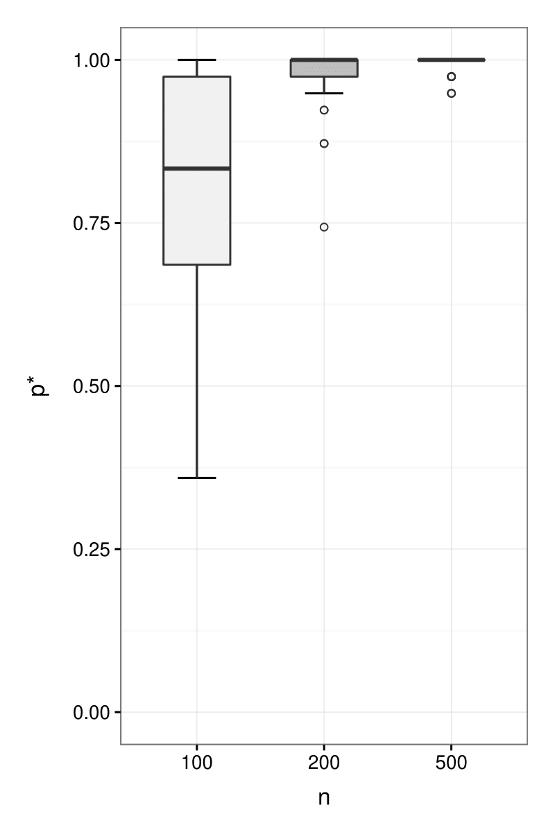
Figure 2: Simulations. Distribution across 40 simulated datasets of the proportion of predictors $p^{*}$ that are correctly classified given a threshold for edge inclusion $k^{*}=0.5$ for each combination of number of nodes $q\in\{20,40\}$ and sample size $n\in\{100,200,500\}$.

We now focus on causal effect estimation. Under each simulated DAG $\mathcal{D}$ and parameters $(\bm{D}^{\mathcal{D}},\bm{L}^{\mathcal{D}})$ we first compute the (true) covariance matrix $\bm{\Sigma}^{\mathcal{D}}$ using (5). Now recall from (13) that the causal effect on $Y$ is a probability which also depends on the level $\tilde{x}$ assigned to the intervened variable $X_{s}$. For each intervened node $s\in\{2,\dots,q\}$ we evaluate $\beta_{s}(\tilde{x},\bm{\Sigma}^{\mathcal{D}},\theta_{0})\equiv\beta_{s}^{true}(\tilde{x})$ at each observed value of $X_{s}$ in the simulation scenario, $(x_{1,s},\dots,x_{n,s})$, and obtain the $(n,1)$ vector of causal effects $\big{(}\beta_{s}^{true}(x_{1,s}),\dots,\beta_{s}^{true}(x_{n,s})\big{)}^{\top}$. Next we produce the collection of BMA estimates $\hat{\beta}_{s}^{BMA}(x_{1,s}),\dots,$ $\hat{\beta}_{s}^{BMA}(x_{n,s})$ according to Equation (27). To evaluate the performance of our method in estimating the causal effect we consider the differences $\big{(}\beta_{s}^{true}(x_{i,s})-\hat{\beta}_{s}^{BMA}(x_{i,s})\big{)}$ and compute the mean absolute error (MAE)

$$MAE_{s}=\frac{1}{n}\sum_{i=1}^{n}\big{|}\beta_{s}^{true}(x_{i,s})-\hat{\beta}_{s}^{BMA}(x_{i,s})\big{|},$$

for each intervened node $s=2,\dots,q$. Results are summarized in the box-plots of Figure 3, where we report the distribution of the MAE (constructed across the $40$ DAGs and nodes $s=2,\dots,q$) as a function of $n$. As expected, MAE decreases and approaches $0$ as the sample size $n$ grows for both values of $q$. Notice that the median value of MAE in the worst case scenario $(q=20,n=100)$ is about half of one percent.

$\quad\quad q=20$	$\quad\quad q=40$

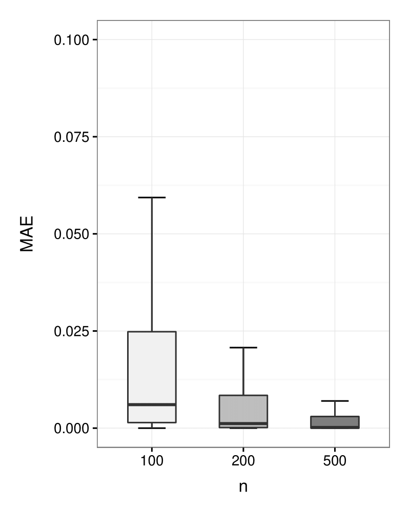
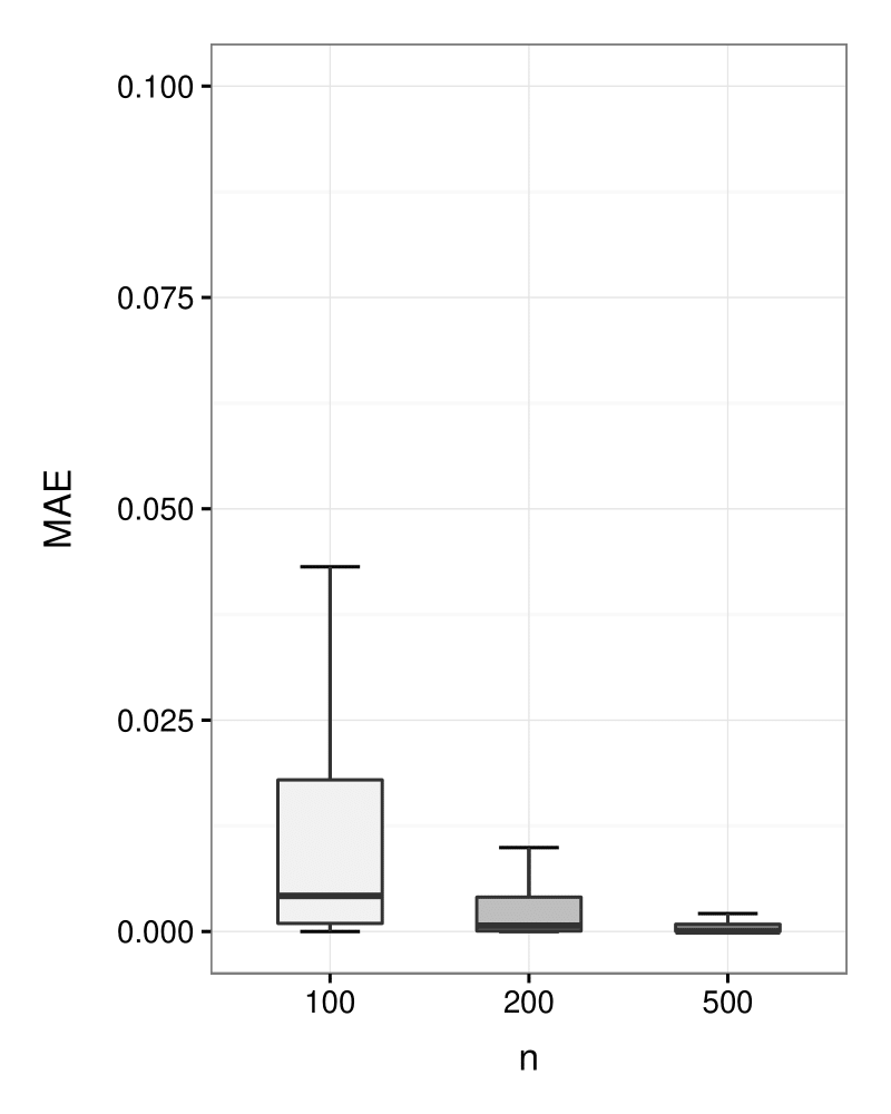
Figure 3: Simulations. Distribution over $40$ datasets and nodes $s\in\{2,\dots,q\}$ of the mean absolute error (MAE) of BMA estimates of true causal effects. Results are presented for each combination of number of nodes $q\in\{20,40\}$ and sample size $n\in\{100,200,500\}$.

Finally, we also explore settings where $n\leq q$: in particular we include simulation results for $q=40$ and $n\in\{10,20,40\}$. Again, we generate $40$ DAGs and the allied parameters as in our first simulation study. Results are summarized in the box-plots of Figure 4, where we report the distribution of the MAE, constructed across the 40 DAGs and nodes $s\in\{2,\dots,q\}$) as a function of $n$. It appears that, even if sample sizes are moderate, MAE decreases as $n$ grows.

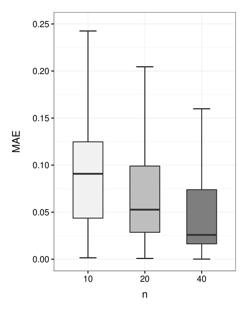
Figure 4: Simulations. Distribution over 40 datasets and nodes $s\in\{2,\dots,q\}$ of the mean absolute error (MAE) of BMA estimates of true causal effects. Results are presented for number of nodes $q=40$ and sample size $n\in\{10,20,40\}$.

7 Analysis of gene expressions from breast cancer cells

In this section we apply our method to a gene expression dataset presented in Yin et al. (2014). The aim of the original study was to evaluate the ability of a gene signature derived from breast cancer stem cells to predict the risk of metastasis and survival in breast cancer patients. To this end, a collection of genes which are believed to be the main responsible for tumor initiation, progression, and response to therapy was considered. The study was motivated by recent literature establishing the existence of a rare population of cells, called stem-like cells, which supposedly represent the cellular origin of cancer; see for instance O’Brien et al. (2006). Gene-expression levels were measured on $n=198$ breast cancer patients of which $62$ manifested distant metastasis. In the following we consider the expression levels of $q=28$ genes included in the original study and a binary response variable $Y$ indicating the occurrence (absence or presence, respectively $Y=0$ and $Y=1$) of distant metastasis. Evaluating the causal effect on $Y$ due to an hypothetical intervention on a specific gene which sets its expression level may help understand which genes are particularly relevant for determining distant metastasis. This in turn can be useful to identify external interventions, which are known to induce variations in the expression of specific genes. For instance epigenetic modifications of gene expressions may be induced by lifestyle and environmental factors such as nutrition-dietary components, exercise, physical activity and toxins; see Abdul et al. (2017). Similarly Campbell et al. (2017) examine the effects of lifestyle interventions on proposed biomarkers of lifestyle and cancer risk at the level of adipose tissue in humans.

We apply Algorithm 1 by fixing the number of MCMC iterations $T=120000$. Observations from the continuous variables $X_{2},\dots,X_{q}$ were standardized. We also set $g=1/n$ and $a=q+1$ in the prior on the Cholesky parameters of $\bm{\Omega}$ as in the simulation scenarios of Section 6. We first use the MCMC output to estimate the posterior probability of inclusion of each directed edge $u\rightarrow v$, that we report in the heat map of Figure 5. Results show a substantial degree of sparsity in the underlying graph structure and only $48$ edges have a posterior probability of inclusion exceeding $0.5$. Moreover, among the 28 genes, only gene IL8, for which $\hat{p}_{\textnormal{\,IL8}\rightarrow Y}(\cdot)=0.70$, seems to directly affect the response variable.

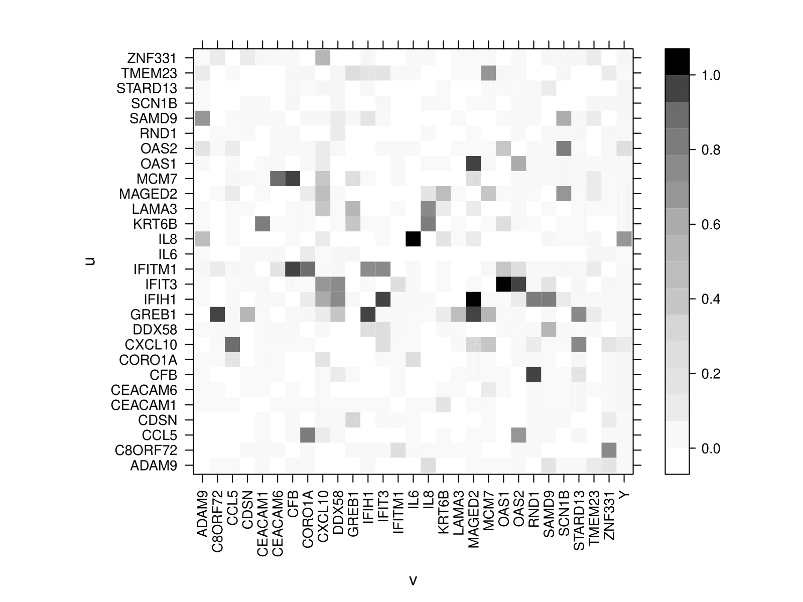
Figure 5: Gene expression data. Heat map with estimated marginal posterior probabilities of edge inclusion for each edge $u\rightarrow v$.

To evaluate the incidence of each gene on the probability of recurrence we compute the causal effect (13) on the response due to an intervention on a specific gene. To this end, starting from the MCMC output we produce a BMA estimate $\hat{\beta}^{BMA}_{s}(\tilde{x})$ for each gene $s=2,\dots,q$ according to (27). Since the causal effect depends on the level $\tilde{x}$ assigned to the intervened variable $X_{s}$, we evaluate $\hat{\beta}^{BMA}_{s}(\tilde{x})$ at each observed value of $X_{s}$, that is $x_{1,s},\dots,x_{n,s}$. The results are reported in Figure 6, where each box-plot refers to a gene $s\in\{2,\dots,q\}$ and summarizes the distribution of $n=198$ BMA estimates, $\big{\{}\hat{\beta}^{BMA}_{s}(x_{i,s})\big{\}}_{i=1}^{n}$. Because the data were standardized, the ranges of $X_{2},\dots,X_{q}$ are similar and we can meaningfully compare results across genes.

Recall from Proposition 3.1 that $\gamma_{s}$ is the covariance between $X_{s}$ and $X_{1}$. If $\gamma_{s}=0$, Equation (13) shows that the causal effect on $Y$ due to an intervention on $X_{s}$ does not vary with $\tilde{x}$. If prior information is weak in relation to the sample size, the estimate of the causal effect will be close to the overall frequency of distant metastasis in the sample (0.31). This is the situation exhibited by most genes in Figure 6. On the other hand if $\gamma_{s}$ is not zero, the collection of causal effects evaluated at $x_{is}$, $i=1,\ldots,n$ will vary. Since the observations are centred, their average is zero and the causal effects will be spread around the value corresponding to the average $\bar{x}_{s}=0$ whose estimate is 0.31 as indicated above. This is what happens for a few genes such as IL8, OAS2 and KRT6B, which exhibit a much greater variability of the causal effect across their measurements, implying that their regulation can influence the occurrence of distant metastasis. In particular, gene IL8 has also been identified as having a potential impact on cancer cells in several studies (Waugh & Wilson, 2008). Other genes which stand out in terms of variability are OAS2 and KRT6B, with the latter not directly linked to $Y$ (as one can see from the heat map of Figure 5) and exhibiting a moderate causal effect on $Y$ which is likely due to the strong association of KRT6B with IL8 (as it emerges from the posterior probabilities of edge inclusion in Figure 5).

For genes IL8 and OAS2 we also report in Figure 7 more detailed results for causal effect estimation. In particular, each plot reports the BMA estimates $\big{\{}\hat{\beta}^{BMA}_{s}(x_{i,s})\big{\}}_{i=1}^{n}$ (represented by $n=198$ dots), and the corresponding credible regions at level $95\%$ represented by the grey area. Results show that increasing expression levels of IL8 are likely to increase the presence of distant metastasis, with BMA estimates of the probability of recurrence ranging in the interval $[0.18;0.54]$. This is consistent with results we have obtained showing that most of the mass of the distribution of the coefficient $\gamma_{s}$ for these genes is assigned to the positive half-line; see also the discussion after (13). Moreover, more extreme levels of IL8 are associated with larger credible regions. A similar behavior, although less pronounced, is observed for gene OAS2 with BMA estimates ranging between $[0.25;0.41]$.

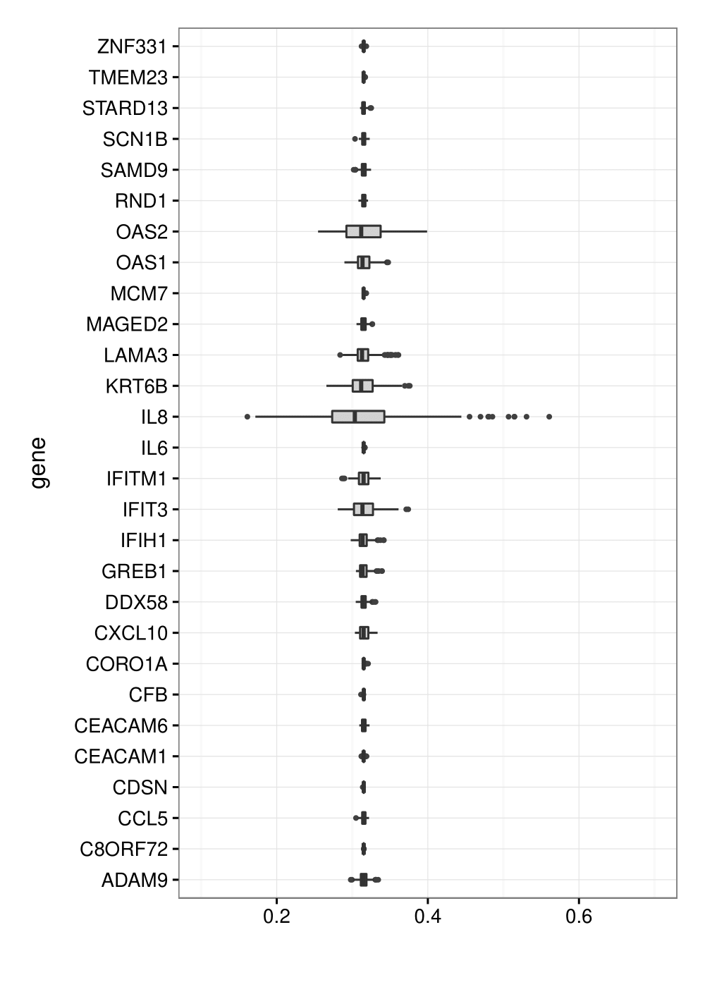
Figure 6: Gene expression data. Box-plots of BMA estimate of causal effect. Each box-plot refers to one of the 28 genes $s$, and represents the $n=198$ BMA estimates computed at each observed value $(x_{1,s},\dots,x_{n,s})$ of expression for gene $s$.

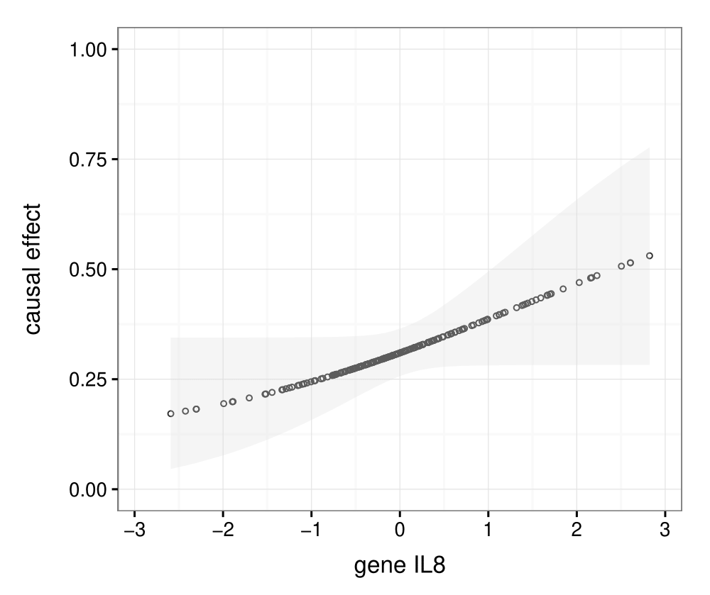
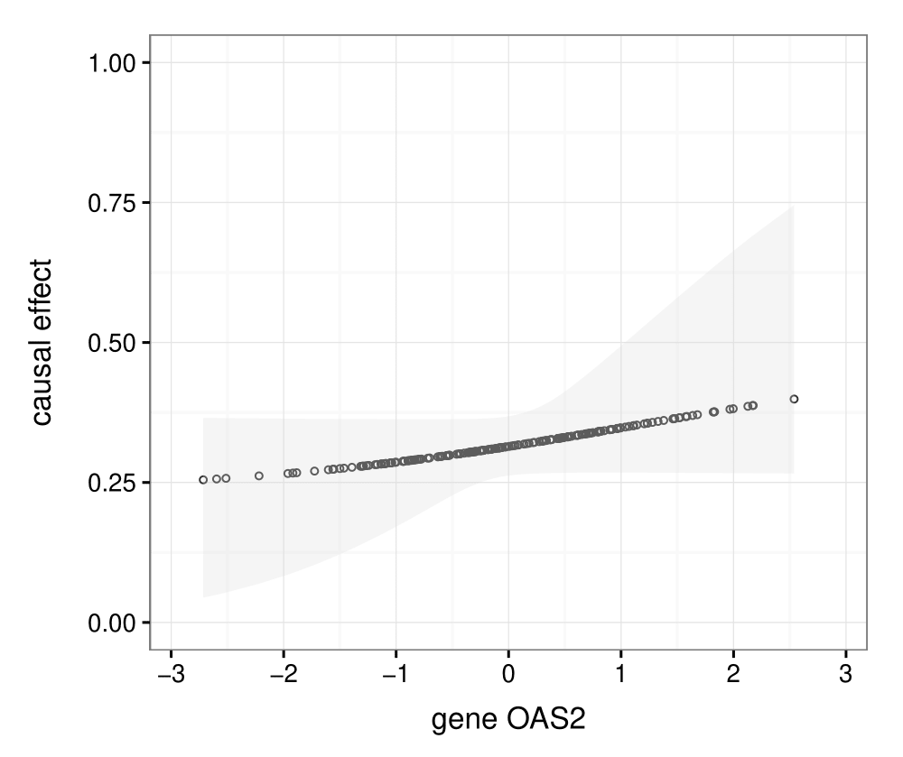
Figure 7: Gene expression data. BMA estimates (dots) and credible regions at level $95\%$ (grey area) for two selected genes, IL8 and OAS2.

8 Discussion

In this paper we deal with causal effect estimation from observational data. We consider a system of real-valued variables together with a binary response; interest lies in the evaluation of the causal effect on the response due to an external intervention on a variable. We assume that the response is generated by standard thresholding applied to a continuous latent variable, and assume that the joint distribution of all continuous variables belongs to a zero-mean Gaussian Directed Acyclic Graph (DAG) model, or equivalently a Structural Equation Model (SEM), and name the resulting model DAG-probit.

Rather than constructing a prior distribution on the covariance (or precision) matrix constrained by a given DAG, we proceed by assigning to the corresponding Cholesky parameters a DAG-Wishart prior whose hyperparameters are deduced from a single unique Wishart distribution. This technique not only drastically simplifies prior elicitation, but has the important advantage of producing score equivalence, meaning that marginal likelihoods of Markov equivalent DAG models are all equal (Geiger & Heckerman, 2002). This feature will have a useful implication, as we discuss at the end of this section.

Because the structure of the data-generating DAG is unknown, we construct an MCMC sampler whose target is the joint posterior distribution of the DAG and the allied Cholesky parameters. This is achieved by carefully tailoring a Partial Analytic Structure (PAS) algorithm to our DAG setting. As a by-product, we recover the MCMC sequence of causal effects corresponding to each visited DAG; this represents the input to our final Bayesian Model Averaging (BMA) estimate, which naturally accounts for model uncertainty on the underlying graph structure.

The assumption of jointly normally distributed random variables can be a source of concern whenever one faces a concrete data analysis. With regard to our application the Gaussian assumption has been often used to analyse gene expression data; see for instance Dobra et al. (2004) and Markowetz & Spang (2007). In addition, it allows to easily incorporate the binary outcome through a latent component, and results in an efficient algorithm, because of closed-form expressions both for the posterior distribution of parameters, as well as for the marginal likelihood of models.

Besides the assumption of normality, our model posits a unique graphical structure as the generating mechanism of all observations. Nevertheless, some problems may suggest to partition the units into groups each having a specific graphical structure which can be however related to the other ones, as in gene expressions collected on multiple tissues from the same individual (Xie et al., 2017). In this setting a multiple graphical model setup would be more appropriate to encourage similarities between group graphical structures; see for instance Peterson et al. (2015) for a Bayesian analysis of multiple Gaussian undirected graphical models. The latter could be a useful starting point for an extension of our DAG-probit model to multiple groups.

In this work we consider causal effects as obtained from interventions on single nodes. However in practice an exogenous intervention may affect many variables (genes) simultaneously and accordingly one may want to predict for instance the effect of a double or triple gene knockout on the response. Causal effect estimation from joint interventions is carried out in a Gaussian setting by Nandy et al. (2017) using a frequentist approach. Their results show that the causal effect of $X_{s}$ on the response in a joint intervention on a given set of variables can be still expressed as a function of the covariance matrix Markov w.r.t. $\mathcal{D}$. The same problem can be tackled by adopting a Bayesian methodology which combines DAG structural learning and causal effect estimation and is currently under investigation by ourselves. In addition, an extension to DAG-probit models should be feasible along the lines of this paper.

The methodology adopted in this work revolves around DAGs. However, it is known that in the Gaussian setting DAGs encoding the same conditional independencies (Markov equivalent DAGs) are not distinguishable using observational data (Verma & Pearl, 1990) and can be collected into Markov equivalence classes (MECs). Accordingly, when the goal of the analysis is structural learning (model selection) MECs represent the appropriate inferential object (Andersson et al., 1997). However, if the objective is causal effect estimation, this is no longer so, because Markov equivalent DAGs may return distinct causal effects. An inspection of (13) reveals the reason: a causal effect depends on the parent set of the intervened node, and this may differ among DAGs within the same MEC. Yet MECs can be exploited also for causal inference, as we now detail. In a frequentist setting, Maathuis et al. (2009) first estimate a MEC using the classic PC algorithm (Spirtes et al., 2000), and then provide an estimate of the causal effect under each DAG within the estimated equivalence class. Alternatively, a Bayesian methodology would first determine the posterior distribution on MEC space, and then, conditionally on a given MEC, compute the posterior of each causal effect within the class (one for each DAG). A single MEC causal effect estimate can be obtained by averaging effects across DAGs, using uniform weights on equivalent DAGs. Finally, an overall Bayesian Model Averaging (BMA) estimate can be obtained by averaging MEC-conditional estimates using posterior probabilities of MECs as weights; for details see (Castelletti & Consonni, 2020a). We remark that the above strategies require an exhaustive enumeration of all DAGs belonging to a MEC, which is not feasible even for a moderate number of nodes. Accordingly one considers only the distinct causal effects within a given MEC, because these values can be efficiently recovered (Maathuis et al., 2009, Algorithm 3) even in high-dimensional settings. In this work we seemingly ignore the issue of DAG Markov equivalence, and propose a causal inference procedure which directly focuses on DAG space, rather than MEC space. However, as already remarked at the beginning of this section, our method for parameter prior construction across DAG models guarantees score equivalence for DAGs within the same MEC. This, together with a uniform prior on DAGs within the same MEC, ensures that causal effects associated to Markov equivalent DAGs will be assigned equal weights in the resulting BMA estimate.

References

- Abdul et al. (2017) Abdul, Q., Yu, B., Chung, H., Jung, H. & J.S., C. (2017). Epigenetic modifications of gene expression by lifestyle and environment. Archives of Pharmacal Research 40 1219–1237. URL https://doi.org/10.1007/s12272-017-0973-3.
- Albert & Chib (1993) Albert, J. H. & Chib, S. (1993). Bayesian analysis of binary and polychotomous response data. Journal of the American Statistical Association 88 669–679. URL http://www.jstor.org/stable/2290350.
- Andersson et al. (1997) Andersson, S. A., Madigan, D. & Perlman, M. D. (1997). A characterization of Markov equivalence classes for acyclic digraphs. The Annals of Statistics 25 505–541. URL http://dx.doi.org/10.1214/aos/1031833662.
- Barbieri & Berger (2004) Barbieri, M. M. & Berger, J. O. (2004). Optimal predictive model selection. The Annals of Statistics 32 870–897. URL https://doi.org/10.1214/009053604000000238.
- Ben-David et al. (2015) Ben-David, E., Li, T., Massam, H. & Rajaratnam, B. (2015). High dimensional Bayesian inference for Gaussian directed acyclic graph models. arXiv pre-print URL https://arxiv.org/abs/1109.4371.
- Campbell et al. (2017) Campbell, K. L., Landells, C. E., Fan, J. & Brenner, D. R. (2017). A systematic review of the effect of lifestyle interventions on adipose tissue gene expression: Implications for carcinogenesis. Obesity 25 S40–S51. URL https://onlinelibrary.wiley.com/doi/abs/10.1002/oby.22010.
- Cao et al. (2019) Cao, X., Khare, K. & Ghosh, M. (2019). Posterior graph selection and estimation consistency for high-dimensional Bayesian DAG models. The Annals of Statistics 47 319–348. URL https://doi.org/10.1214/18-AOS1689.
- Castelletti & Consonni (2020a) Castelletti, F. & Consonni, G. (2020a). Bayesian inference of causal effects from observational data in Gaussian graphical models. Biometrics, In press .
- Castelletti & Consonni (2020b) Castelletti, F. & Consonni, G. (2020b). Supplementary material to “Bayesian causal inference in probit graphical models” .
- Dobra et al. (2004) Dobra, A., Hans, C., Jones, B., Nevins, J. R., Yao, G. & West, M. (2004). Sparse graphical models for exploring gene expression data. Journal of Multivariate Analysis 90 196 – 212. URL http://www.sciencedirect.com/science/article/pii/S0047259X04000259.
- Friedman (2004) Friedman, N. (2004). Inferring cellular networks using probabilistic graphical models. Science 303 799–805. URL https://science.sciencemag.org/content/303/5659/799.
- Friedman & Koller (2003) Friedman, N. & Koller, D. (2003). Being Bayesian about network structure. A Bayesian approach to structure discovery in Bayesian networks. Machine Learning 50 95–125. URL https://doi.org/10.1023/A:1020249912095.
- García-Donato & Martínez-Beneito (2013) García-Donato, G. & Martínez-Beneito, M. A. (2013). On sampling strategies in bayesian variable selection problems with large model spaces. Journal of the American Statistical Association 108 340–352. URL https://doi.org/10.1080/01621459.2012.742443.
- Geiger & Heckerman (2002) Geiger, D. & Heckerman, D. (2002). Parameter priors for directed acyclic graphical models and the characterization of several probability distributions. The Annals of Statistics 30 1412–1440. URL https://doi.org/10.1214/aos/1035844981.
- Godsill (2012) Godsill, S. J. (2012). On the relationship between markov chain monte carlo methods for model uncertainty. Journal of Computational and Graphical Statistics 10 230–248. URL https://doi.org/10.1198/10618600152627924.
- Guo et al. (2015) Guo, J., Levina, E., Michailidis, G. & Zhu, J. (2015). Graphical models for ordinal data. Journal of Computational and Graphical Statistics 24 183–204. URL https://doi.org/10.1080/10618600.2014.889023.
- Lauritzen (1996) Lauritzen, S. L. (1996). Graphical Models. Oxford University Press.
- Maathuis & Nandy (2016) Maathuis, M. & Nandy, P. (2016). A review of some recent advances in causal inference. In P. Bühlmann, P. Drineas, M. Kane & M. van der Laan, eds., Handbook of Big Data. Chapman and Hall/CRC, 387–408.
- Maathuis et al. (2009) Maathuis, M. H., Kalisch, M. & Bühlmann, P. (2009). Estimating high-dimensional intervention effects from observational data. The Annals of Statistics 37 3133–3164. URL https://doi.org/10.1214/09-AOS685.
- Markowetz & Spang (2007) Markowetz, F. & Spang, R. (2007). Inferring cellular networks - a review. BMC Bioinformatics 8. URL https://doi.org/10.1186/1471-2105-8-S6-S5.
- Nandy et al. (2017) Nandy, P., Maathuis, M. H. & Richardson, T. S. (2017). Estimating the effect of joint interventions from observational data in sparse high-dimensional settings. Ann. Statist. 45 647–674. URL https://doi.org/10.1214/16-AOS1462.
- O’Brien et al. (2006) O’Brien, C. A., Pollett, A., Gallinger, S. & Dick, J. E. (2006). A human colon cancer cell capable of initiating tumour growth in immunodeficient mice. Nature 445 106–110. URL https://doi.org/10.1038/nature05372.
- Pearl (1995) Pearl, J. (1995). Causal diagrams for empirical research. Biometrika 82 669–688. URL http://www.jstor.org/stable/2337329.
- Pearl (2000) Pearl, J. (2000). Causality: Models, Reasoning, and Inference. Cambridge University Press, Cambridge.
- Pearl (2009) Pearl, J. (2009). Causal inference in statistics: An overview. Statistics Surveys 3 96–146. URL https://doi.org/10.1214/09-SS057.
- Peters & Bühlmann (2014) Peters, J. & Bühlmann, P. (2014). Identifiability of Gaussian structural equation models with equal error variances. Biometrika 101 219–228. URL http://www.jstor.org/stable/43305605.
- Peterson et al. (2015) Peterson, C., Stingo, F. C. & Vannucci, M. (2015). Bayesian inference of multiple Gaussian graphical models. Journal of the American Statistical Association 110 159–174. PMID: 26078481, URL https://doi.org/10.1080/01621459.2014.896806.
- Spirtes et al. (2000) Spirtes, P., Glymour, C. & Scheines, R. (2000). Causation, Prediction and Search (2nd edition). Cambridge, MA: The MIT Press.
- Verma & Pearl (1990) Verma, T. & Pearl, J. (1990). Equivalence and synthesis of causal models. In Proceedings of the Sixth Annual Conference on Uncertainty in Artificial Intelligence, UAI 90. New York, NY, USA: Elsevier Science Inc., 255–270.
- Wang & Li (2012) Wang, H. & Li, S. Z. (2012). Efficient gaussian graphical model determination under g -wishart prior distributions. Electronic Journal of Statistics 6 168–198. URL https://doi.org/10.1214/12-EJS669.
- Waugh & Wilson (2008) Waugh, D. J. & Wilson, C. (2008). The interleukin-8 pathway in cancer. Clinical Cancer Research 14 6735–6741. URL https://doi.org/10.1158/1078-0432.CCR-07-4843.
- Xie et al. (2017) Xie, Y., Liu, Y. & Valdar, W. (2017). Joint estimation of multiple dependent Gaussian graphical models with applications to mouse genomics. Biometrika 103 493–511. URL https://doi.org/10.1093/biomet/asw035.
- Yin et al. (2014) Yin, Z.-Q., Liu, J.-J., Xu, Y.-C., Yu, J., Ding, G.-H., Yang, F., Tang, L., Liu, B.-H., Ma, Y., Xia, Y.-W., Lin, X.-L. & Wang, H.-X. (2014). A 41-gene signature derived from breast cancer stem cells as a predictor of survival. Journal of Experimental & Clinical Cancer Research 33. URL https://doi.org/10.1186/1756-9966-33-49.