Supplementary material for
Imaging phonon-mediated hydrodynamic flow in WTe₂

Extended Data Fig. 1: a Temperature dependent resistivity at zero magnetic field. The residual resistivity ratio (RRR) between 300 K and 2 K is $\sim 2000$, signifying the high quality of the single crystal. b Magnetic field (applied along the $\hat{c}$-axis) dependent resistivity showing Shubnikov-de Haas oscillations at 2 K. c The fast Fourier transform (FFT) of the background-subtracted data of (b) when plotted against the inverse of the magnetic field. We notice four fundamental peaks corresponding to the extremal orbits of the electron and hole pockets in the Brillouin zone Zhu et al. (2015).

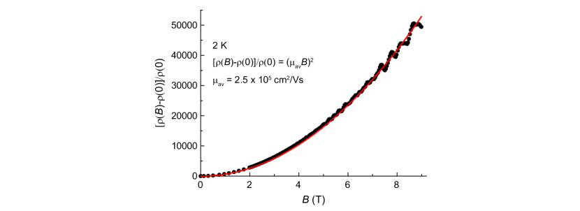
Extended Data Fig. 2: Fitting of the magnetic field dependent resistivity at 2 K according to the relation $\frac{\rho(B)-\rho(0)}{\rho(0)}=(\mu_{av}B)^{2}$ where $\mu_{av}$ is the average mobilityZhu et al. (2015); Ali et al. (2015). This allows us to extract $\mu_{av}=2.5\times 10^{5}~{}\mathrm{cm^{2}/Vs}$. Using the relation $\sigma=\mu ne$, the average carrier density $n=1.47\times 10^{20}~{}\mathrm{cm^{-3}}$ can be extracted.

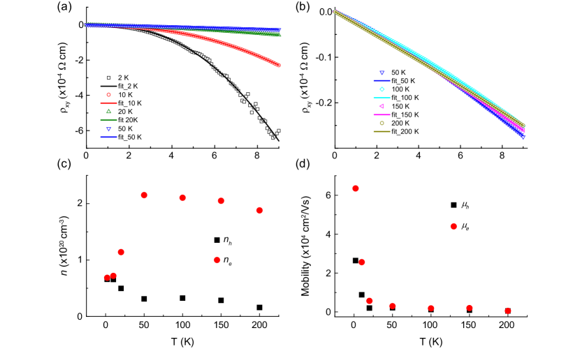
Extended Data Fig. 3: a, b Hall resistivity vs. magnetic field measured at different temperatures. The data is fitted according to the two-band model $\rho_{yx}=\frac{B}{e}\frac{(n_{h}\mu_{h}^{2}-n_{e}\mu_{e}^{2})+(n_{h}-n_{e})\mu_{h}^{2}\mu_{e}^{2}B^{2}}{(n_{h}\mu_{h}+n_{e}\mu_{e})^{2}+(n_{h}-n_{e})^{2}\mu_{h}^{2}\mu_{e}^{2}B^{2}}$ Luo et al. (2015); Zhao et al. (2015). c Carrier density of electrons and holes vs. temperature, extracted from the fits in (a) and (b). d Mobility of electrons and holes vs. temperature, extracted from the fits in (a) and (b).

Extended Data Fig. 4: Optical image of the WTe₂ sample used for the majority of the data in the manuscript, including Main text Fig. 2, 3, and 4. The $100~{}\mathrm{\mu m}$ long flake is contacted at its ends with gold contacts. The path along which our magnetic field profiles were taken is shown in white. An additional gold line nearby is used for delivery of RF power to manipulate the NV.

Extended Data Fig. 5: a An optical image of our scanning tip. A quartz rod is glued to the edge of one of the prongs of a quartz tuning fork. A diamond cube of $50\times 50\times 125~{}\mathrm{\mu m}$ is glued to the other side of the rod. b A closeup image of the diamond cube, with a $3~{}\mathrm{\mu m}$ etched pillar visible. This pillar is used as our scanning probe, and an NV defect is located $~{}20~{}\mathrm{nm}$ away from the pillar edge.

Extended Data Fig. 6: a A schematic for multiple pillar sensing. The diamond is tilted at an angle $\theta$ (using goniometric motors) so that one pillar is in contact with the substrate, while the scanning pillar maintains a constant height above the sample without touching it. The angle $\theta$ control the height of the NV probe above the sample. b An optical image of a multiple pillar scanning tip with 7 pillars. The extreme pillars are made to be thicker so they are optimized for durability in contact, while the central pillars are optimized for NV sensing.

1 Echo magnetometry

There are several ways to extract the magnetic field from the NV defect, and here we will describe the method used in the paper, which utilizes the long coherence of the NV as a quantum sensor.

The NV electron spin is a spin-1 system, and its low energy state are the triplet states $\left|-1\right>=\left|\downarrow\downarrow\right>$, $\left|0\right>=\frac{1}{\sqrt{2}}(\left|\uparrow\downarrow\right>+\left|\downarrow\uparrow\right>)$, and $\left|1\right>=\left|\uparrow\uparrow\right>$. The $\left|0\right>$ is split in energy from $\left|-1\right>$ and $\left|1\right>$ by the zero field splitting and $\left|-1\right>$ and $\left|1\right>$ are split by applying a bias magnetic field due to Zeeman splitting. We apply an external bias field of $1650~{}\mathrm{G}$ parallel to the NV axis, where the energy splitting between the $\left|-1\right>$ and $\left|0\right>$ states is $1.7~{}\mathrm{GHz}$. This is the only transition used in our experiment, and so the system can now be described as a qubit made of these two states.

An external magnetic field parallel to the NV axis shifts the frequency of our qubit by $g\mu_{B}B_{||}$ due to the Zeeman effect, where $g\sim 2$ is the NV g-factor, $\mu_{B}$ is the Bohr magneton, and $B_{||}$ is the applied parallel magnetic field. This shift is approximately $2.87~{}\mathrm{MHz/G}$. Measuring the resonance frequency of the qubit allows us to infer the local parallel magnetic field.

This frequency is often measured by a continuous spectroscopy method (ESR) in which the NV is probed with RF radiation at different frequencies to find the frequency at which the NV is excited, leading to reduced red counts in the optical measurement. While this method is simple, it has several drawbacks. The continuous drive can heat up the system being measured, and lead to broadening of the resonance peak. Also, the contrast in this measurement is halved as the states compared are $\left|0\right>$ and an equal mixture of $(\left|0\right>,\left|-1\right>)$ as opposed to full contrast between $\left|0\right>$ and $\left|-1\right>$. Another method is Ramsey interferometry, in which the qubit is placed in a superposition state $\frac{1}{\sqrt{2}}(\left|0\right>+i\left|-1\right>)$. This superposition evolves to acquire a phase $\frac{1}{\sqrt{2}}(\left|0\right>+ie^{i\Delta t}\left|-1\right>)$ due to the change $\Delta$ in the qubit resonance frequency. A measurement of this phase provides the shift in resonance frequency and therefore the magnetic field. This technique requires pulsed control, and thus overcomes many of drawbacks of continuous spectroscopy. The time over which we can acquire a phase is limited by the low frequency qubit coherence time $T_{2}^{*}$.

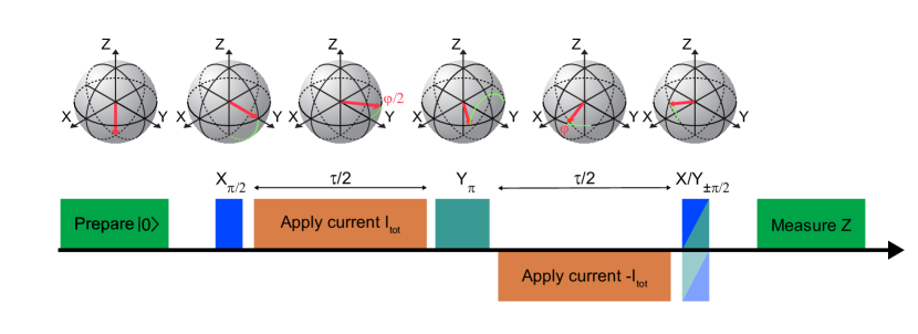
Fig. S1: A schematic of our echo magnetometry experiment. The pulses applied are shown below in sequence, and the Bloch sphere representation above shows the state of the qubit at the corresponding place in the sequence. The red arrow indicates the current state of the qubit, while the green line indicates the path it took on the Bloch sphere since the last step. A detailed description of the sequence can be found in Section 3. For the last $\pi/2$, there are four possible rotations, and the Bloch sphere representation shows the $\pi/2$ around the X-axis.

Pulsed manipulation of the qubit allows for more complicated sequences which cancel the effect of low frequency noise, improving the qubit coherence time from $T_{2}^{*}$ to $T_{2}$. In this experiment we used the simplest such sequence, the echo experiment, as shown in detail in Supplementary Fig. S1. The qubit is initially prepared in the $\left|0\right>$ state by illuminating green light. Afterwards, an RF pulse is applied to perform a $\pi/2$ pulse around the X-axis. This places the qubit in the superposition state $\frac{1}{\sqrt{2}}(\left|0\right>+i\left|-1\right>)$. Then a current $I_{tot}$ is applied along the device for a duration $\tau/2$. This current leads to a parallel magnetic field $B_{||}$ and thus to a frequency shift $\Delta=g\mu_{B}B_{||}$ in the qubit resonance frequency shift. During a time $\tau/2$ a phase $\varphi/2=\Delta\tau/2$ is acquired by the qubit, which is then left in the state $\frac{1}{\sqrt{2}}(\left|0\right>+ie^{\varphi/2}\left|-1\right>)$. A $\pi$ pulse around the Y-axis is then applied on the qubit, leading to the state $\frac{1}{\sqrt{2}}(\left|-1\right>-ie^{\varphi/2}\left|0\right>)=\frac{1}{\sqrt{2}}(\left|0\right>+ie^{-\varphi/2}\left|-1\right>)$. Note that the phase accumulated has been reversed and so applying the same current again will lead to a cancellation of the acquired phase. Instead we apply the opposite current, leading to an acquisition of an additional $-\varphi/2$ phase, leading to the state $\frac{1}{\sqrt{2}}(\left|0\right>+ie^{-\varphi}\left|-1\right>)$. The phase has now been acquired and we need to extract it. For this, we repeat this experiment with four different pulse options: $\pi/2$ pulse around X-axis, $\pi/2$ pulse around the Y-axis, $-\pi/2$ pulse around the X-axis, and $-\pi/2$ pulse around the Y-axis. For each option we then measure the $Z$ component of the qubit by applying green laser light and collecting red photons. From the 4 measurements of probabilities to be in the $\left|-1\right>$ state collected after their respective pulses we can extract $\varphi$ as:

$$\varphi=\arctan\left(\frac{M_{X\pi/2}-M_{X-\pi/2}}{M_{Y-\pi/2}-M_{Y\pi/2}}\right),$$ (S1)

where $M_{X\pi/2}$ is the measurement following the $\pi/2$ pulse around the X-axis and respectively for the others. The different measurements allow us to cancel the effect of background counts and focus only on the optical contrast due to the qubit state.

Note that this sequence is only useful for sensing alternating magnetic fields, where the field frequency is equal to the echo frequency. This is useful in current measurement where we can lock the application of current to the echo measurement, but is not useful for measuring static magnetic fields due to magnetization.

As mentioned above, this measurement cancels low frequency noise and thus allows us to acquire a signal up to $\tau=T_{2}$ as opposed to $T_{2}^{*}$. The probe we used had long coherence time $T_{2}=150~{}\mathrm{\mu s}$ (and $T_{2}^{*}=3~{}\mathrm{\mu s}$). However, as will be discussed in Section 6, our measurements were taken at shorter times $\tau=21~{}\mathrm{\mu s}$. This was chosen because we can afford to use relatively high current, for which a longer integration time would lead to phase accumulation significantly above $2\pi$ - leading to ambiguity in the magnetic field as we can only determine the phase up to $2\pi$.

2 Magnetic noise estimations of the NV detector

The measurements that are shown in the main text had to be measured in exceptional signal-to-noise ratio (SNR) in order to observe the slight changes over a small temperature range. In order to achieve that, we made use of a combination of relatively high current $(15-20~{}{\mu}A)$ together with our long echo time (${\approx}20~{}{\mu}s$). In this section we will try to estimate quantitatively the SNR that we have in our measurements. The signal (in $\mathrm{Counts/s}$) is given by:

$$Signal={\Delta}{\phi}{\cdot}C{\cdot}F{\cdot}T{\cdot}N_{Avg},$$ (S2)

where ${\Delta}{\phi}$ is the accumulated phase in the echo experiment, $C$ is the contrast, $F$ is the fluorescence of the NV in $\mathrm{Counts/s}$ , $T$ is the avalanche photo-diode (APD) acquisition time, and $N_{Avg}$ is the number of averages per second. The noise in the system is assumed to be only shot noise:

$$Noise=\sqrt{F{\cdot}T{\cdot}N_{Avg}}.$$ (S3)

We want to calculate the sensitivity per second, assuming a SNR of 1:

$$\frac{Signal}{Noise}=1={\Delta}{\phi}{\cdot}C{\cdot}\sqrt{F{\cdot}T}{\cdot}\sqrt{N_{Avg}}$$ (S4)

From that we can extract the minimal ${\Delta}{\phi}$:

$${\Delta}{\phi}=\frac{1}{C{\cdot}\sqrt{F{\cdot}T}}{\cdot}\frac{1}{\sqrt{N_{Avg}}}$$ (S5)

In order to estimate the smallest magnetic field, we need to convert phase to field via:

$${\Delta}B={\Delta}{\phi}{\cdot}\frac{1}{2{\pi}{\gamma}}{\cdot}\frac{1}{{\tau}},$$ (S6)

where $\Delta B$ is the magnetic field, $\tau$ is the spin-echo time, and ${\gamma}=g{\cdot}{\mu}_{B}=2.87~{}\frac{\mathrm{MHz}}{\mathrm{Gauss}}$ where $g$ is the g-factor and ${\mu}_{B}$ is the permeability of the vacuum. From that we get:

$${\Delta}B=\frac{1}{2{\pi}{\gamma}{\cdot}C\sqrt{F{\cdot}T}}{\cdot}\frac{1}{{\tau}}{\cdot}\frac{1}{\sqrt{N_{Avg}}}$$ (S7)

To estimate the magnetic noise, we can approximate (by ignoring overheads and assuming long enough ${\tau}$) $N_{Avg}{\approx}\frac{1}{{\tau}}$ (where we assume the total time spent measuring is $1~{}\mathrm{s}$). From that we get:

$$B_{noise}{\approx}\frac{1}{2{\pi}{\gamma}{\cdot}C\sqrt{F{\cdot}T}}{\cdot}\frac{1}{\sqrt{{\tau}}}$$ (S8)

In our NV center $C=0.15$ , $F=120{\cdot}10^{3}~{}\mathrm{Counts/s}$ , $T=300~{}\mathrm{ns}$, and for our experiments in the main text ${\tau}=21.2~{}\mathrm{{\mu}s}$. From these values we can estimate the magnetic field noise level:

$$B_{noise}=43~{}\mathrm{\frac{nT}{\sqrt{Hz}}}$$ (S9)

By comparing to theory, we empirically estimate of the noise in the magnetic field profile of the gold contact in Main text Fig. 2 and get:

$$B_{noise}=104~{}\mathrm{\frac{nT}{\sqrt{Hz}}}$$ (S10)

The additional noise can be attributed to mechanical noise and other overheads. In our measurements, in order to reduce the noise even further we were averaging over $10~{}\mathrm{s}$ which gives a noise of ${\Delta}B{\approx}13~{}\mathrm{nT}$. Together with a signal of ${\sim}5~{}\mathrm{{\mu}T}$ (peak to peak in Main text Fig. 2b without normalization) we get an estimate of the SNR of:

$$\frac{Signal}{Noise}~{}{\approx}~{}384$$ (S11)

We also want to extract from this magnetic noise the minimal current density that is possible to detect using our probe. Assuming a simple rectangular current profile, we can use the $B_{z}$ profile from Main text Fig. 2b, where we applied ${\sim}13~{}\mathrm{{\mu}A}$ when the device width is $1.7~{}\mathrm{{\mu}m}$ and got ${\sim}5~{}\mathrm{{\mu}T}$ peak to peak. To achieve a SNR of $1$ for a $10~{}\mathrm{s}$ measurement, we get the minimal current density:

$${\Delta}J~{}{\approx}~{}20~{}\mathrm{\frac{nA}{{\mu}m}}$$ (S12)

By taking advantage of our long $T_{2}$ and measuring for $150~{}\mathrm{{\mu}s}$ echo time, we are able to decrease this number even more and get:

$${\Delta}J~{}{\approx}~{}7.3~{}\mathrm{\frac{nA}{{\mu}m}}$$ (S13)

3 Cuts along the gold contact at different temperatures

In Main text Fig. 2c, the cuts along the gold line is used as a control which shows Ohmic flow, as opposed to the WTe₂ current profile. In Main text Fig. 3, we show the temperature dependence of the current profile in WTe₂. The current profile of the gold contact is expected to be Ohmic at all temperatures. To verify this point, we measure the flow profile at 90 K and 10 K and they are shown in Supplementary Fig. S2. The similarity between the two curves is comparable to our noise level, unlike the WTe₂ profiles which show a significant deviation.

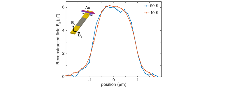
Fig. S2: Reconstruction of the magnetic field $B_{x}$ as a function of the position along the gold contact, taken at 90 K and 10 K.

4 Finding the same line-cut at different temperatures

In Main text Fig. 3 we have shown a dependence of the current profile on temperature. Due to mechanical deformations (thermal expansion) of the scanning system at different temperatures, we had to determine the exact location along the device to perform the scan for every temperature. We first used our optical microscope to determine the position roughly (up to a few microns). Following that, we performed a scan along the device (Inset, Supplementary Fig. S3) while keeping the tip at the center of the device. A point along the device happened to have a strong distortion of the current which manifested as a peak in the Rabi frequency at this point. In Supplementary Fig. S3 the measured Rabi frequency as a function of position is shown and a clear peak is visible at around $Y=0~{}\mathrm{\mu m}$. The peak serves as a marker, and for each temperature we performed our scan at the same distance ($2.7~{}\mathrm{\mu m}$) from the peak (dashed vertical lines Supplementary Fig. S3). Using this technique, we were able to verify the location along the device for every current profile scan in Main text Fig. 3.

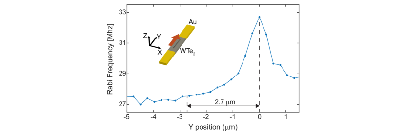
Fig. S3: Rabi frequency measured as a function of the position along y direction while keeping the x position along the center of the device. The peak is indicated by dashed line and measured $2.7~{}\mathrm{\mu m}$ away another dashed line indicates the position in which we performed the x scan (the scan in figure 3 of the main text).

5 Temperature dependence of current profile: additional data

To verify the reproducibility of the non-monotonic current profile temperature dependence shown in Main text Fig. 3, we took additional cuts at different $Y$ positions along the sample. One such set of cuts is shown in Supplementary Fig. S4. Note that these line cuts were taken without the careful $Y$ alignment procedure described in the previous section. Thus, the data shown in the Main text is more reliably free from measurement artefacts.

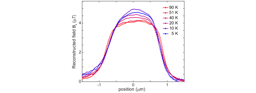
Fig. S4: Reconstruction of the magnetic field $B_{x}$ as a function of the position for various temperatures. Additional data showing non-monotonic temperature dependence.

6 Flow profile dependence on current

The bias applied on the WTe₂ that was used throughout the paper was chosen to be small enough that it is in the linear response regime yet large enough that the signal to noise ratio is maximized.

In order to verify linear response, we performed two scans with two different currents, one scan with relatively high current ($19~{}\mathrm{\mu A}$) and one scan with relatively low current ($4.7~{}\mathrm{\mu A}$). Importantly, to preserve the signal to noise ratio, we performed the two scans with different corresponding echo times to accumulate the same final phase (see Section 3 for details on AC magnetometry). For the high current scan, we used a $21~{}\mathrm{\mu s}$ phase accumulation time and for the low current scan we used $86~{}\mathrm{\mu s}$ (which is the same ratio between the current amplitudes). As a result, the low current scan was $~{}4$ times longer.

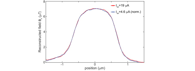
Fig. S5: Reconstructed magnetic field $B_{x}$ as a function of the position along the device, taken for two different current amplitudes. The red curve corresponds to a scan with a current of $19~{}\mathrm{\mu A}$ and measured with an echo time of $86~{}\mathrm{\mu s}$. The blue curve corresponds to a scan with current of $4.6~{}\mathrm{\mu A}$ and measured with an echo time of $86~{}\mathrm{\mu s}$. Both measurements were taken at $12~{}\mathrm{K}$.

The results can be seen in Supplementary Fig. S5, as two $B_{x}$ magnetic field profiles are shown. The blue one was taken with high current and the red with low current. As can be clearly seen, the difference between the two curves is very small which means that indeed we are in the linear response regime. So, in order to maximize signal to noise ratio and to avoid drifts of the mechanical scanning system over long scanning times we used the high current $19~{}\mathrm{\mu A}$ and $21~{}\mathrm{\mu s}$ echo time throughout the paper.

7 Magnetic field profile sample thickness dependence

In Main Text Fig. 2a,b we compare our data with the magnetic field profiles generated by the current profiles shown in Main Text Fig. 2c at our probe height. We use the approximation of current flowing in a 2D sheet, not accounting for our sample thickness of $60~{}\mathrm{nm}$.

To confirm that this is a good approximation, we show in Supplementary Fig. S6 the magnetic field profiles $B_{x}$ and $B_{z}$ generated by a uniform current profile for a 2D sheet (red line) and a $60~{}\mathrm{nm}$ thick sample (blue line). The good agreement between the profiles justifies our approximation.

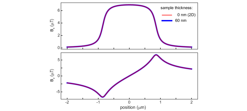
Fig. S6: Spatial profiles of the $B_{x}$ and $B_{z}$ magnetic field components generated by uniform current flow at the probe height $h=140~{}\mathrm{nm}$ above the sample. The red line corresponds to a 2D sample with no thickness, while the blue line corresponds to a thickness of $60~{}\mathrm{nm}$. For the blue line, the height $h$ is measured from the center of the sample. The blue line is intentionally thicker so both curves are visible.

8 Fourier magnetic field reconstruction

The energy splitting of the NV electron spin states are sensitive to the component of the magnetic field parallel to the NV axis. However, under certain conditions we can extract the full magnetic field vector from such a measurementBlakely (1996); Lima and Weiss (2009); Casola et al. (2018). This allowed us to reconstruct the $B_{x}$ component of the magnetic field, as shown in Main text Figs. 2c and 3.

The NV used in our experiment was oriented in the y-z plane. As the current flows along the y-axis, only the z-axis magnetic field component $B_{z}$ contributes field parallel to our NV. Thus, our NV directly measures $B_{z}$ as we scan above the sample, up to a factor of $1/\sqrt{3}$ due to the angle of the NV in the y-z plane.

We measure the magnetic field in a plane above the sample. Assuming all sources of magnetic field are below our plane, for the magnetic field in the plane we can assume source-free magnetism: $\nabla\cdot\vec{B}=0$ and $\nabla\times\vec{B}=0$. These additional equations allow us to extract the full vector $\vec{B}$ from a single component. The full derivation is covered in the previous references, and here we focus on the special case of extracting $B_{x}$ from $B_{z}$ which was used in our measurement. The equations then reduce to the simple form:

$$b_{x}(k_{x},k_{y},z)=-i\frac{k_{x}}{\sqrt{k_{x}^{2}+k_{y}^{2}}}b_{z}(k_{x},k_{y},z)$$ (S14)

where $k_{x}$, $k_{y}$ are the $x$ and $y$ components of the planar wave vector, and $b_{x/z}(k_{x},k_{y},z)=\int_{-\infty}^{\infty}\int_{-\infty}^{\infty}B_{x/z}(x,y,z)\allowbreak e^{-i(k_{x}x+k_{y}y)}dxdy$ is the 2D Fourier transform of $B_{x/z}$ on the plane. Thus, in Fourier space $B_{x}$ and $B_{z}$ are related by a simple factor, allowing us to extract the perpendicular $B_{x}$ component of the magnetic field.

For our analysis, we used the profile measured along the 1D path (x-axis) above the sample, and assumed the magnetic field pattern was constant along the y-axis. Note that in Main text Fig. 2b, the magnetic field is still finite at the edge of our scanning window. As the Fourier integral required the field on the entire plane, this was problematic for the reconstruction. To improve our analysis, we extrapolated both edges of our scan with fits to $1/x$ tails before applying the reconstruction.

9 Electron hydrodynamics overview: Nomenclature, regimes and relevant derivations

At high temperatures, electron transport is usually resistive. This is in large part due to the numerous momentum-relaxing scattering events, the microscopics of which are discussed below. Macroscopically, this leads to the well-known constitutive relation known as Ohm’s ‘law’, and can be described within the Drude theory of metals. At very low temperatures the electron mean-free path, the average distance electrons travel in between scattering events, can exceed the geometry’s length scale leading to ballistic behavior. In certain materials, there exists a collective-transport regime in between these two limits whereby mean free paths are low, suggesting numerous scattering events, but momentum is on-average conserved following scattering. This collective-transport behavior is commonly referred to as hydrodynamic flow due to the resemblance of the resulting flow signatures to classical hydrodynamics. While experimentally these transport regimes are observed as a function of temperature, a more natural choice for non-dimensional independent variables is the ratio of the momentum-relaxing and momentum-conserving mean free paths to the geometry’s length scale ($l_{mr}(T)/W$, $l_{mc}(T)/W$). Note that these depend implicitly on temperature.

9.1 Electronic Boltzmann transport equation

In the absence of momentum-conserving scattering, the steady-state evolution of non-equilibrium electron distribution functions is given, at the relaxation time approximation (RTA) level, by:

$$\boldsymbol{v}_{s}\cdot\nabla_{\boldsymbol{r}}f(s,\boldsymbol{r})+e\boldsymbol{E}\cdot\nabla_{s}f(s,\boldsymbol{r})=-\frac{f(s,\boldsymbol{r})-\bar{f}(s)}{\tau_{s}^{mr}},$$ (S15)

where $f(s,\boldsymbol{r})$ is the non-equilibrium distribution of electrons around position $\boldsymbol{r}$ with state label $s$ (encapsulating the wavevector $\boldsymbol{k}$ and band index $n$). Non-equilibrium electrons are allowed to drift in space with a particular group velocity, $\boldsymbol{v}_{s}$, as a result of an external forcing term, where $e$ is the electron charge and $\boldsymbol{E}$ is an externally-applied electric field. These drifting electrons undergo momentum-relaxing events with an lifetime, $\tau_{s}^{mr}$, which acts to returns them towards an equilibrium distribution $\bar{f}(s)$.

We investigate the flow signatures eq. S15 permits in a two-dimensional channel, making the common assumption of a circular Fermi surface de Jong and Molenkamp (1995). Due to translational invariance along the channel, eq. S15 simplifies to read:

$$v_{y}\partial_{y}F(y,\theta)-eE_{x}v_{x} =-\frac{F(y,\theta)-\langle F(y)\rangle_{\theta}}{\tau_{mr}}$$ (S16)

$$\sin(\theta)\partial_{y}F(y,\theta)+\frac{F(y,\theta)}{l_{mr}} =eE_{x}\cos(\theta),$$ (S17)

where we have introduced the linearized electron deviation, $F(y,\theta)$, via $f(y,\theta)\approx f_{0}-\left(\frac{\partial f_{0}}{\partial\epsilon}\right)F(y,\theta)$, and used $\boldsymbol{v}=v_{F}\binom{\cos(\theta)}{\sin(\theta)}$, $\langle F(y)\rangle_{\theta}=0$, and $l_{mr}=\tau_{mr}v_{F}$, where $v_{F}$ is the Fermi velocity, in simplifying the last line. Finally, since eq. S17 is linear, we seek normalized solutions of the form: $F(y,\theta)=eE_{x}\cos(\theta)\,l_{eff}(y,\theta)$ by solving:

$$\sin(\theta)\partial_{y}\,l_{eff}(y,\theta)+\frac{l_{eff}(y,\theta)}{l_{mr}}=1,$$ (S18)

This allows a natural definition for an ‘average’ mean free path $\tilde{l}_{eff}(y)$, which is directly proportional to current density, $j_{x}(y)$:

$$\tilde{l}_{eff}(y) =\int_{0}^{2\pi}\frac{d\theta}{\pi}\cos^{2}(\theta)l_{eff}(y,\theta)$$ (S19)

$$j_{x}(y) =\left(\frac{m}{\pi\hbar^{2}}\right)E_{F}e^{2}\frac{E_{x}}{mv_{F}}\tilde{l}_{eff}(y)$$ (S20)

Equation S18 can be readily solved using appropriate boundary conditions, which we take to be completely diffuse, i.e.

$$z\forall_{\theta}\in[0,\pi) \qquad l_{eff}(-W/2,\theta)=\frac{1}{\pi}\int_{\pi}^{2\pi}d\theta^{\prime}l_{eff}(-W/2,\theta^{\prime})=\mathrm{const}=0$$ (S21)

$$\forall_{\theta}\in[\pi,2\pi) \qquad l_{eff}(W/2,\theta)=\frac{1}{\pi}\int_{0}^{\pi}d\theta^{\prime}l_{eff}(W/2,\theta^{\prime})=\mathrm{const}=0,$$ (S22)

where $W$ is the channel width, and the constant value at the boundary can be chosen as zero at zero magnetic field Sulpizio et al. (2019).

9.2 Ballistic to diffusive transition

Supplementary Fig. S7a plots the solution to eq. S20 for various values of the first non-dimensional parameter, namely $l_{mr}/W$. It is instructive to identify the two limits. As $\lim_{l_{mr}/W\to 0}$, i.e. the electrons undergo multiple momentum-relaxing scattering events before reaching the edge of the geometry, we recover a uniform ‘Ohmic’ profile, with zero current density at the boundaries. At the other extreme, as $\lim_{l_{mr}/W\to\infty}$, i.e. electrons reach the edge of the geometry without undergoing any scattering, we recover the (essentially) uniform ‘Knudsen’ profile, with nonzero current density at the boundaries. In between the two limits, we observe a non-diffusive current profile, which peaks when $l_{mr}\sim W$. Note that, in contrast with the ‘Gurhzi’ flows described below, the current density remains nonzero at the boundary.

9.3 Hydrodynamic to diffusive transition

Before introducing momentum-conserving terms in our electronic BTE, it is instructive to approach the problem from the opposite direction, i.e. introduce momentum-relaxing terms to a pure hydrodynamic solution. To this end, our starting point is the electronic Stokes equation:

$$-\nu\partial^{2}_{y}\,j_{x}(y)+\tau_{mr}^{-1}\,j_{x}(y)=\frac{ne^{2}E_{x}}{m},$$ (S23)

where $\nu=l_{mc}v_{F}$ is an effective electron viscosity, $n$ is the carrier density, and $m$ is the electron effective mass. Using the (stricter) no-slip boundary conditions, i.e. $j_{x}(\pm W/2)=0$, the solution to eq. S23 is given by:

$$j_{x}(y) =\frac{e^{2}l_{mr}}{\hbar}\sqrt{\frac{n}{\pi}}E_{x}\left(1-\frac{\cosh(x/D)}{\cosh(W/2D)}\right)$$ (S24)

$$=\frac{I_{total}}{W-2D\tanh(W/2D)}\left(1-\frac{\cosh(x/D)}{\cosh(W/2D)}\right),$$ (S25)

where $D=\sqrt{l_{mc}l_{mr}}$ is the geometric average of the momentum-conserving and momentum-relaxing mean free paths called the ‘Gurzhi’ length, and we have normalized all the physical constants with the total current, $I_{total}$.

Supplementary Fig. S7b plots the solution to eq. S23 for various values of the non-dimensional parameter $D/W$. As in the ‘Knudsen’ case, as $\lim_{D/W\to 0}$ we recover a uniform ‘Ohmic’ profile, with $j_{x}(y)=\frac{I_{total}}{W}$. By contrast, as $\lim_{D/W\to\infty}$ we instead recover a fully parabolic ‘Poiseuille’ profile, with $j_{x}(y)=\frac{3I_{total}(1-4y^{2})}{2W}$. Note that, by virtue of our stringent boundary conditions, all solutions exhibit zero current density at the boundary and the peak current is monotonically increasing as $D/W$ increases. Both these observations are in stark contrast with our experimental observations, and thus we turn back to the electronic BTE.

Fig. S7: a Normalized current density solutions to the momentum-relaxing electronic BTE as a function of $l_{mr}/W$, the value of which is denoted by color. The profiles transition from uniform diffusive flow (at low $l_{mr}/W$), to non-diffusive flow (at $l_{mr}\sim W$), to ballistic ‘Knudsen‘ flow (at high $l_{mr}/W$). This is quantified by the curvature of the current (inset), peaking at 0.25. b Normalized current density solutions to the electronic Stokes as a function of $D/W$. The profiles transition monotonically from uniform diffusive flow (at low $D/W$), to parabolic ‘Poiseuille’ flow (at high $D/W$). c Comparison of experimental profiles with the ab initio profiles afforded within the ‘Knudsen‘ picture, showing poorer agreement as compared to Main Fig. 4c.

9.4 Momentum-conserving BTE

We seek to add additional scattering terms to eq. S18, which on-average conserve momentum:

$$\int_{0}^{2\pi}d\theta v_{x}\left.\frac{\partial l_{eff}(y,\theta)}{\partial t}\right|_{mc}=0$$ (S26)

The simplest possible such term is given by de Jong and Molenkamp (1995):

$$\sin(\theta)\partial_{y}\,l_{eff}(y,\theta)+\frac{l_{eff}(y,\theta)}{l_{mr}}=1+\left(-\frac{l_{eff}}{l_{mc}}+\frac{\tilde{l}_{eff}}{l_{mc}}\right)$$ (S27)

$$\sin(\theta)\partial_{y}\,l_{eff}(y,\theta)+\frac{l_{eff}(y,\theta)}{l}=1+\frac{\tilde{l}_{eff}}{l_{mc}},$$ (S28)

where the first additional term ‘depopulates’ electrons according to an average mean free path $l_{mc}$ and the second term enforces these electrons are redistributed appropriately to conserve momentum. In the last line, we use Mathhiessen’s rule $l^{-1}=l_{mc}^{-1}+l_{mr}^{-1}$ to combine the mean free path terms. Note that the presence of $\tilde{l}_{eff}$ in eq. S28 makes our equation integro-differential. We solve this using both an iterative and an integral solver, to avoid numerical instabilities of each method.

9.5 Experimental comparison against ballistic limit

Since the purely ballistic picture also permits non-diffusive flows which can exhibit non-monotonic curvature behavior, we compare the experimental results using eq. S20. This is shown in Supplementary Fig. S7c, which should be compared with Main Fig. 4c. First, note that the temperature peak is shifted from $\sim 15\mathrm{K}$ to $\sim 20\mathrm{K}$. Second, the non-monotonic temperature dependence requires substantially purer samples. Finally, we note that the experimental profiles are more curved than the maximum curvature afforded by the ‘Knudsen‘ picture.

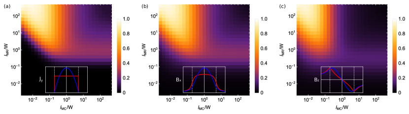
Fig. S8: a Current density curvature phase diagram for various values of $l_{mc(mr)}/W$. Inset shows the two curvature bounds for diffusive and parabolic flows respectively. b Normalized $B_{x}$ peak value phase diagram for various values of $l_{mc(mr)}/W$. Inset shows the $B_{x}$ profiles for diffusive and parabolic flows, which acts as our normalizing lower and upper bounds respectively. Note how the $B_{x}$ profile for diffusive flow is not flat, due to the finite height of the NV above the sample. c Normalized $B_{z}$ extremum position phase diagram for various values of $l_{mc(mr)}/W$. Inset shows the $B_{z}$ profiles for diffusive and parabolic flows, which acts as our normalizing lower and upper bounds respectively. Note that for diffusive flow the $B_{z}$ extrema positions align with the sample edge, and move inwards for curved profiles.

9.6 Current density profiles quantification

The solutions to eqs. S20 and S28 yield the current density as a function of position. In Main Fig.4, we summarize our results on a two-dimensional phase diagram, quantifying the profiles using a scalar metric. In this section, we discuss the various choices for scalar metrics and their slight differences. Supplementary Fig. S8a plots the current density’s curvature as a function of $l_{mc(mr)}/W$. While this is a natural choice, which is by construction normalized, we do not have direct access to the current density from our experiments. Also note that the current density exhibits a sharp transition between the ‘porous’ (bottom left) and hydrodynamic regimes (top left), making the differentiation of in-between regimes challenging. By contrast, our measurements are sensitive to the magnetic field induced by this current density above the sample, and we plot the $B_{x}$ and $B_{z}$ components in Supplementary Fig. S8b-c respectively. The two metrics are very similar, but we prefer to use the normalized peak value of the $B_{x}$ profile since its connection to the current density is more intuitive.

Fig. S9: a Overall effective mean free path for various values of $l_{mr(mc)}/W$. Note the density plot is clipped at $L_{eff}/W=5$, to emphasize the regions of interest. Overlaid arrows represent ab initio trajectories. b One-dimensional cuts of (a) for fixed values of $l_{mr}/W$, illustrating the possibility of non-monotonicity. c ab initio extracted conductivity, showing monotonic temperature dependence.

9.7 Electrical conductivity

A physical scalar representation of the current density, available using transport measurements, is the conductivity in the channel given by:

$$\sigma=\frac{ne^{2}}{m^{*}v_{F}}\int_{-W/2}^{W/2}\frac{dy}{W}\tilde{l}_{eff}(y)=\frac{ne^{2}}{m^{*}v_{F}}L_{eff},$$ (S29)

where $L_{eff}$ is the overall effective mean free path de Jong and Molenkamp (1995). Supplementary Fig. S9a plots $L_{eff}/W$ for various values of $l_{mr(mc)}/W$, with the ab initio trajectories overlaid as arrows. This indeed allows for non-monotonic behavior, highlighted by the 1D-cuts at fixed values of $l_{mr}/W$ in Supplementary Fig. S9b. While transport measurements of conductivity can in principle extract the non-monotonicity we observe in our spatially-resolved measurements, their dynamical range is different and in-fact our particular sample the non-monotonicity would not be observed. This is highlighted in Supplementary Fig. S9c, which further illustrates the importance of spatially-resolved measurements and theory.

9.8 Anisotropic Fermi Surface

In this section, we relax the assumption of a circular Fermi surface, used throughout the main text and preceding sections, and instead consider a ‘parametric‘ Fermi surface of the form $\boldsymbol{k}=k_{F}\rho(\theta)\binom{\cos(\theta)}{\sin(\theta)}$, where $\rho(\theta)$ is a polar equation defined between $\theta=0$ and $\theta=2\pi$, with an average value of 1. The Fermi velocity is then given by the vector normal to the Fermi wave-vector:

$$\boldsymbol{v}=v_{F}\binom{\cos(\theta)\rho(\theta)+\sin(\theta)\rho^{\prime}(\theta)}{\sin(\theta)\rho(\theta)-\cos(\theta)\rho^{\prime}(\theta)}$$ (S30)

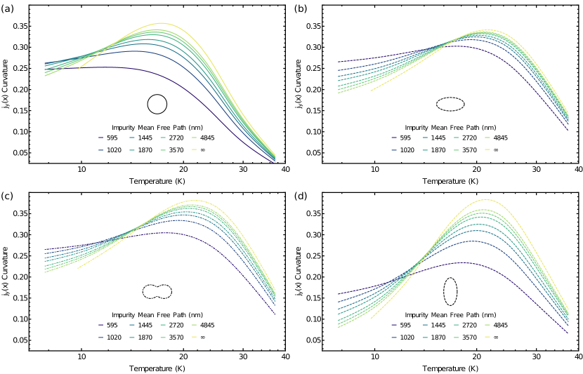
Fig. S10: Current density curvature variation as a function of temperature for systems with a a circular, b elliptical (eccentricity $e=0.875$), and c two-fold anisotropic (anisotropy strength $\epsilon=0.5$) Fermi surfaces. d Comparison between the relative of orientation of the Fermi surface to the channel direction for an elliptical Fermi surface with the same eccentricity as in b.

Note that we naturally recover the circular Fermi surface limit by setting $\rho(\theta)=1$. In particular we consider elliptical Fermi surfaces with an eccentricity $e$ and two-fold parametric Fermi surfaces with an anisotropy strength $\epsilon$, rotated at an angle $\theta_{0}$ with the horizontal axis:

$$\rho_{\mathrm{ellipse}}(\theta) =\sqrt{2}\sqrt{-\frac{\sqrt{1-e^{2}}}{-2+e^{2}+e^{2}\cos[2(\theta-\theta_{0})]}}$$ (S31)

$$\rho_{\mathrm{two-fold}}(\theta) =1+\epsilon\cos[2(\theta-\theta_{0})]$$ (S32)

The derivation of the anisotropic BTE proceeds by generalizing the parametrization in the main text $F(y,\theta)=eE_{x}v_{x}(\theta)\,l_{eff}(y,\theta)$ and using the fact that the drift-velocity along the transverse direction is zero at steady-state to decouple the terms in the integral de Jong and Molenkamp (1995). This leads to an equation of the form:

$$\hat{v}_{y}(\theta)\partial_{y}\,l_{eff}(y,\theta)+\frac{l_{eff}(y,\theta)}{l}=1+\frac{1}{l_{mc}}\int_{0}^{2\pi}\frac{d\theta^{\prime}}{\pi}\hat{v}_{x}^{2}(\theta)l_{eff}(y,\theta^{\prime}),$$ (S33)

which we solve numerically using an iterative finite-element solver. Equation S33 is convention-dominated, which presents numerical difficulties for certain parametric Fermi surfaces exhibiting $\theta$-discontinuities. We address this by adding a small amount ($\approx 5\times 10^{-4}$) of artificial diffusion to the right-hand-side of eq. S33.

Figure S10 plots the current density curvature as a function of temperature for various empirical impurity values (color-code), for different Fermi surface parametrizations. While the temperature non-monotonicity is perserved in all these configurations, with a peak around $15-25$K, the exact position of the peak appears to shift to higher temperatures for non-spherical Fermi surfaces. The effects of introducing both significant anisotropy in the Fermi surface (Fig. S10b) as well as non-convex regions (Fig. S10c) on the range of curvature values achieved appear to be otherwise weak. Finally, we investigated the effect of Fermi surface alignment with the channel direction (Fig. S10d). The increased distribution of Fermi velocity directions aligned with the channel can indeed lead to increased values of curvature Bachmann et al. (2021). While this phenomenon is most pronnounced in the ballistic limit Bachmann et al. (2021), we see remnants of this behavior persist in the regime we’re operating in - with considerable momentum-conserving interactions.

10 Computational details

The ab initio calculations were performed with the open source density functional theory (DFT) code JDFTx Sundararaman et al. (2017). First we fully relaxed the $T_{d}$-WTe₂ (Fig. 1c, main text) using fully relativistic Perdew-Burke-Ernzerhof pseudopotentials Perdew et al. (1996); Dal Corso (2014); Perdew et al. (2008) and Grimme’s D-2 van der Waals approach Grimme (2006). A kinetic cutoff energy of 40 Ha was used along with a $14\times 7\times 4$ Gamma-centered $k$-mesh, and a Fermi-Dirac smearing of 0.01 Ha for the Brillouin zone integration. Both the lattice constants and the ion positions were relaxed until the forces on all atoms were less than 10^-8 Ha/Bohr. The relaxed lattice constants were found to be $a=3.46$ Å, $b=6.20$ Å, and $c=13.09$ Å, respectively. To compute the e-ph scattering time, we performed frozen phonon calculations in a $1\times 1\times 1$ supercell, and obtained 88 maximally localized Wannier functions (MLWFs) by projecting the plane-wave bandstructure to W $d$ and Te $p$ orbitals, which allowed us to converge the electron scattering calculation on a much finer $112\times 56\times 32$ ($224\times 112\times 64$) $\mathbf{k^{\prime}}$ and $\mathbf{q}$ grid for $T>(<)20$ K. $\tau^{\mathrm{PH}}_{\mathrm{ee}}$ was collected on 56 irreducible q points in the Brillouin zone. For e-e scattering, we reduced the $k$-mesh to $6\times 3\times 2$ due to the computational cost, for which we verified the electronic structure. A dielectric matrix cutoff of 120 eV was used to include enough empty states, with a energy resolution of 0.01 eV.

Further, since the electronic structure of $T_{d}$-WTe₂ is known to be sensitive to lattice strain Soluyanov et al. (2015), the Weyl semimetal phase (WSM) was realized by confining the lattice constants to $a=3.48$ Å, $b=6.25$ Å, and $c=14.02$ Å. Here we employed fully relativistic Perdew-Wang Perdew and Wang (1992) pseudopotentials with the same settings as described earlier to obtain stable phonons. An extensive comparison between the Relaxed phase and WSM phase is shown in Sec. 10.

11 Relaxed phase vs. Weyl semimetal phase

As mentioned in the previous section, the WSM phase has $\sim 7$ % tensile strain along the stacking $\hat{z}$ axis. The phonon modes only show slight softening along the $\Gamma-Z$ direction compared to the relaxed structure, without significant difference overall. However, the relaxed phase has much more dispersive electronic structure along $\Gamma-Z$ direction due to a shorter distance between the van der Waals layers (Supplementary Fig. S11(a) and (c)). Consequently, the Fermi energy cuts through these bands, leading to a slightly more ‘metallic’ behavior in the relaxed phase. One may expect leaving a larger hole pocket (Supplementary Fig. S11(b) and (d)). However, when we examine the spatially resolved momentum relaxing electron-phonon lifetimes on the Fermi surface in these two structures, the WSM phase features longer-lived electrons than the relaxed phase.

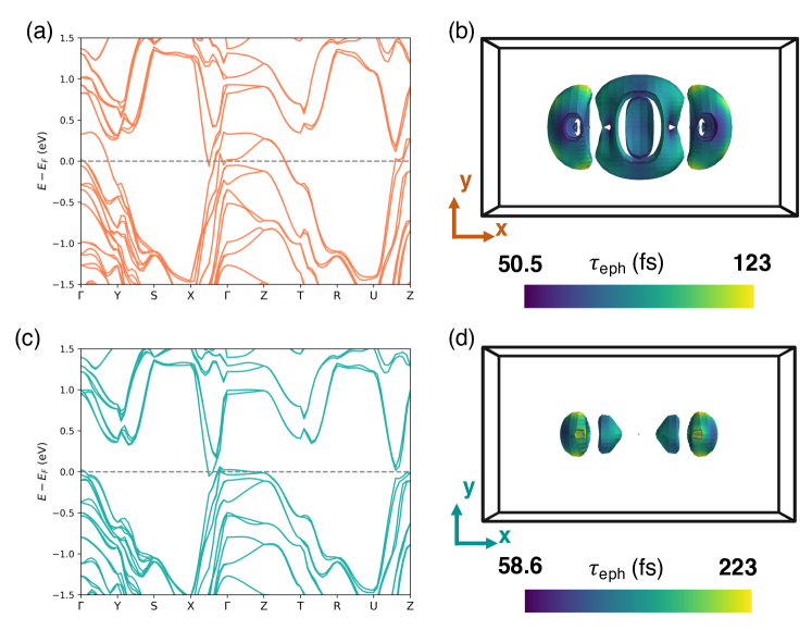
Fig. S11: Electronic bandstructures and Fermi surfaces for relaxed (a-b) and WSM (c-d) WTe₂ phases. In (b) and (d) we show the electron-phonon lifetimes at 28 K projected onto the Fermi surfaces to highlight the anisotropic feature.

To better understand their hydrodynamic behavior, we performed the same numerical calculation with ab initio $\tau_{\rm ee}$, $\tau_{\rm ee}^{\rm PH}$, and $\tau_{\rm eph}$. We found that while $\tau_{\rm mr}$ does not show predominant distinction, $\tau_{\rm ee}$ is greatly decreased in the WSM phase. As a result, the non-monotonic temperature dependence of the resulting current density profiles peaks at $\sim 8\mathrm{K}$, as shown in Supplementary Fig. S12.

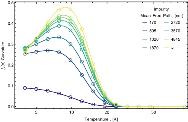
Fig. S12: Ab initio current density curvature solutions as a function of temperature for the Weyl semimetal phase. Note, the peak occurs at a lower temperature, and the curvature values are significantly higher than those observed experimentally.

12 Discussion on high temperature deviations between predicted behavior and experimental observations

As shown in Main Figs. 3,4, the experimental observations above $\sim 40\mathrm{K}$ deviate significantly from the predicted behavior. While the theoretical predictions admit almost entirely diffusive profiles, experimentally we observe curved profiles. In this section, we expand on possible causes for this discrepancy, which can be attributed to approximations made by the theory and experimental uncertainties. First, oxidation effects in the WTe₂ flake result in a non-uniform distribution of impurities, which in turn suggests a position-dependent mean free path. It is instructive to consider the extreme case in which such impurities permit no current density at the edges, effectively reducing the sample width, artificially suggesting enhanced flow in the center. Allowing for $\sim 10\%$ change in the effective width, for example, accounts for the discrepancy at $90~{}\mathrm{K}$. Similarly, while the theoretical model assumes an infinite two-dimensional ribbon, the sample has both finite length ($\sim 100~{}\mathrm{\mu m}$) and finite thickness ($\sim 50~{}\mathrm{nm}$). Since the electron mean free paths (Main Fig. 4a) are of the same order as the sample thickness, this will result in a transition between ‘Knudsen’ and ‘Poiseuille’ flow along the $\hat{z}$ direction, modifying the profiles along the $\hat{x}$ direction. Finally, since our sample is a thin WTe₂ flake exfoliated on a quartz substrate, the phonon spectrum will likely be modified away from that of the bulk crystal. Furthermore, considering the entire WTe₂ phonon spectrum ($<250\mathrm{cm}^{-1}$) is contained within the quartz phonon spectrum, bulk phonons from the WTe₂ can scatter into the substrate with little interface resistance, thus providing another competing scattering mechanism.

13 Electron-Hole Scattering Channels

As indicated by magnetoresistance and Hall resitivity signatures (Figs. S1-S3), WTe₂ is a semimetal with both electron and hole carriers present. In this section we discuss the effect of scattering between the electron and hole pockets on the phonon-mediated time scale ($\tau_{\rm ee}^{\rm PH}$). The identification of different charge carriers in the ab initio calculations is enabled by the well-defined band index used in the maximally localised Wannier functions (MLWFs) formalism, and subsequently adopted in our calculation of the electron phonon matrix elements. To this end, we compute the phonon mediated carrier lifetimes allowing scattering between only the electron (blue) or hole (orange) pockets (Fig. S13), and compare these against the lifetime values obtained allowing for scattering between all bands (red). We note that both momentum and current is conserved for electron-electron and hole-hole scattering, while only momentum is conserved for electron-hole scattering. To address the extent of electron-hole scattering, we use Matthiessen’s rule to sum the contributions assuming electron-electron and hole-hole scattering as independent channels (green curve in Fig. S13). The deviation of the effective lifetime given by Matthiessen’s rule (green) and the computed lifetime using all bands (red) is an indication of how independent these scattering channels are. At the temperatures of interest in this work ($\mathrm{T}\lesssim 90\mathrm{K}$), the two scattering channels are almost entirely independent, and phonon-mediated scattering between electron and hole bands can be neglected.

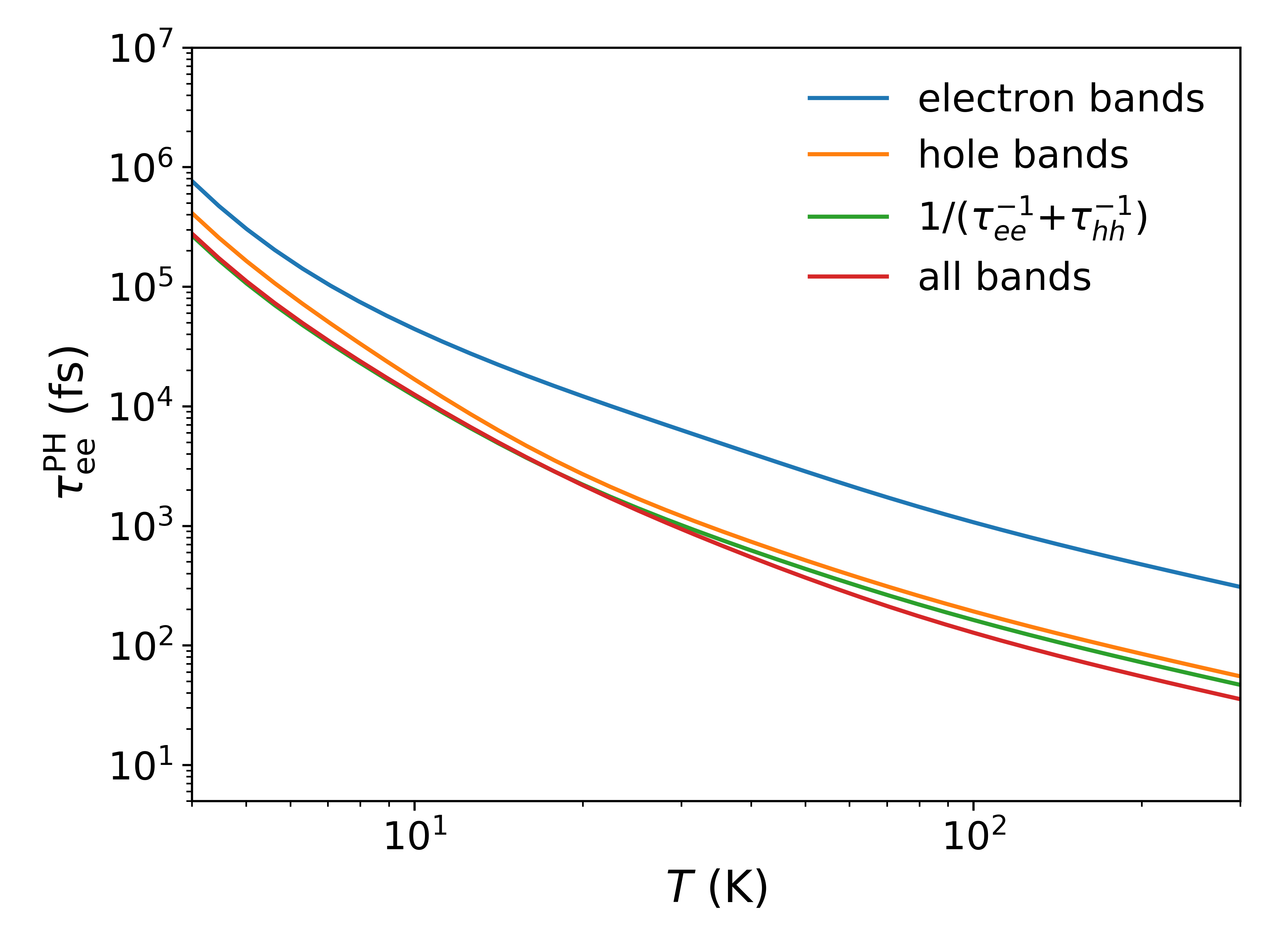
Fig. S13: Phonon mediated carrier lifetimes at different temperatures, computed with all electron bands (blue), all hole bands (orange), and all bands (red), while the green curve is calculated by summing the electron and hole contributions using Matthiessen’s rule.

14 Electron-phonon coupling strength in WTe₂

In this section we calculate the dimensionless coupling strength in WTe₂, which is closely related to the estimation of the critical temperature in phonon-mediated superconductors following the BCS theory McMillan (1968), to facilitate further comparison of WTe₂ with other systems. The electron-phonon coupling strength associated with a specific phonon mode (q$\nu$) can be calculated by

$$\lambda_{\textbf{q}\nu}=\frac{1}{N(\varepsilon_{F})\omega_{\textbf{q}\nu}}\sum_{mn}\int\frac{\mathrm{d}\textbf{k}}{\Omega_{\rm BZ}}|g_{mn,\nu}(\textbf{k,q})|^{2}\times\delta(\varepsilon_{n\textbf{k}}-\varepsilon_{F})\delta(\varepsilon_{m\textbf{k+q}}-\varepsilon_{F}),$$ (S34)

where $N(\varepsilon_{F})$ is the density of states per spin at the Fermi level and other symbols follow the same definition as in the Methods session. The isotropic dimensionless electron-phonon coupling strength ($\lambda$) of WTe₂ is given by the Brillouin zone sum over a uniform $14\times 7\times 4$ q-grid to be 0.49. As means of comparison with a known BCS superconducting system, we obtained $\lambda=\mathbf{0.745}$ on a $12\times 12\times 12$ q-grid for aluminum (superconducting at $T_{C}\approx 1.75$ K), while $\lambda=\mathbf{0.17}$ on a $8\times 8\times 8$ q-grid for copper (non-superconducting).

15 Carrier density effect on the scattering length scales in WTe₂

In layered ver der Waals structures, the Fermi level and thus the carrier density, are sensitive to structural characteristics such as crystal stoichiometry, strain, defects etc. In this section we discuss how differences in carrier density affect the momentum relaxing mean free paths ($l_{mr}$) in WTe₂ through ab initio calculations of both momentum relaxing and momentum conversing length scales through changing the electron chemical potential. For the momentum relaxing length scale, we explicitly examine, how the $\tau_{\rm mr}$ changes at different electron chemical potential, or Fermi level, in WTe₂ for both the WSM phase (solid lines) and the relaxed structure (dashed lines) at multiple temperatures shown in Fig. S14a. Allowing for a chemical potential range within $\pm 200$ meV, we do not see a significant change of $\tau_{\rm mr}$. For the momentum conserving length scale, in this context the phonon-mediated carrier mean free path, the carrier density could affect the phase space for phonon-electron interaction as well as the Brillouin zone integration of ($\tau_{n\textbf{k}}$) since only the states near the Fermi level are required, typically weighted by $-f^{\prime}(\varepsilon_{n\textbf{k}})$ under the Boltzmann relaxation time approximation (RTA). As shown in Fig. S14b, while the contribution from the electron (blue) and hole (orange) carriers could be modified when shifting the chemical potential above the Fermi energy by 50 meV, the change in the overall phonon-mediated length scales (red) is negligible. Therefore, we believe the carrier density will not hinder the intrinsic hydrodynamic limit in WTe₂.

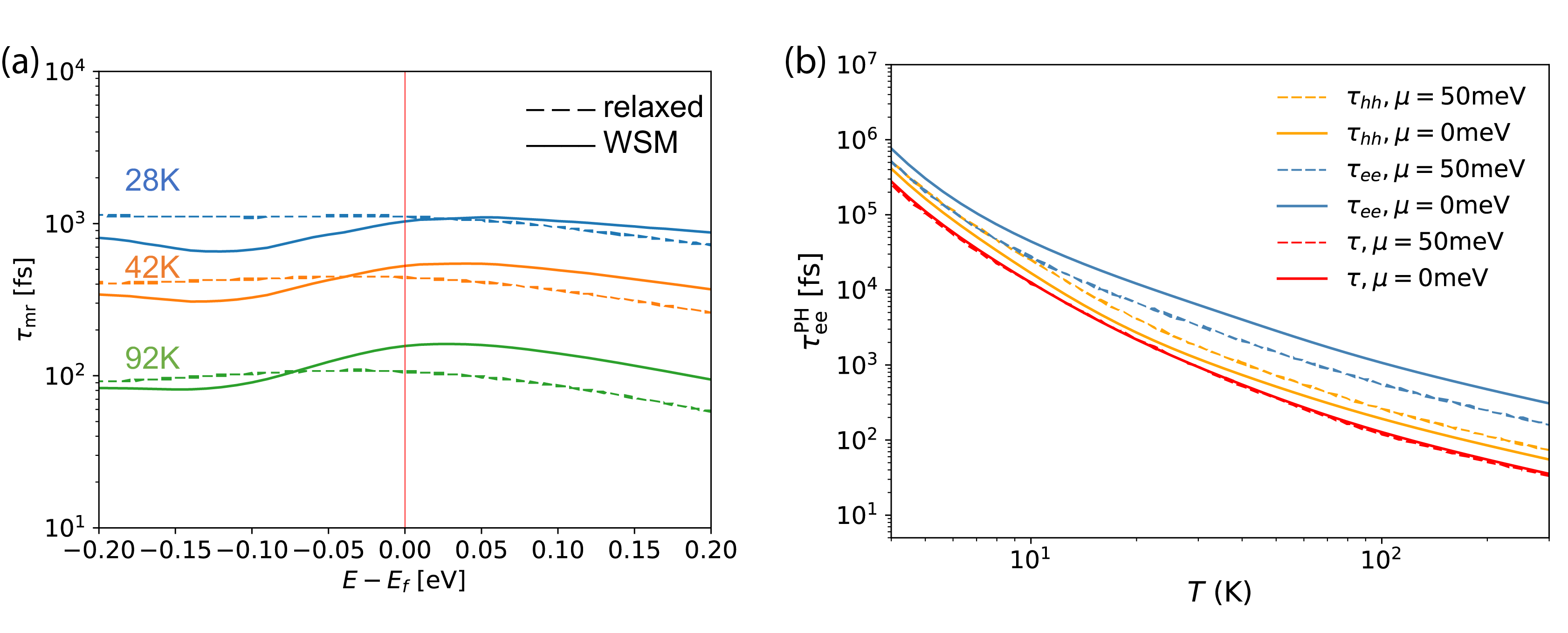
Fig. S14: (a) Momentum relaxing lifetime ($\tau_{\rm mr}$) at different electron chemical potentials at various temperatures (color coded), in both the relaxed structure (dashed lines) and the WSM phase (solid lines). (b) Phonon-mediated carrier lifetimes at different temperatures with a chemical potential shift of 50 meV, computed with all electron bands (blue), all hole bands (orange), and all bands (red).

References

- Zhu et al. (2015) Z. Zhu, X. Lin, J. Liu, B. Fauqué, Q. Tao, C. Yang, Y. Shi, and K. Behnia, Physical Review Letters 114, 176601 (2015).
- Ali et al. (2015) M. N. Ali, L. Schoop, J. Xiong, S. Flynn, Q. Gibson, M. Hirschberger, N. P. Ong, and R. J. Cava, EPL (Europhysics Letters) 110 (2015).
- Luo et al. (2015) Y. Luo, H. Li, Y. M. Dai, H. Miao, Y. G. Shi, H. Ding, A. J. Taylor, D. A. Yarotski, R. P. Prasankumar, and J. D. Thompson, Applied Physics Letters 107, 182411 (2015).
- Zhao et al. (2015) Y. Zhao, H. Liu, J. Yan, W. An, J. Liu, X. Zhang, H. Wang, Y. Liu, H. Jiang, Q. Li, Y. Wang, X.-Z. Li, D. Mandrus, X. C. Xie, M. Pan, and J. Wang, Phys. Rev. B 92, 041104 (2015).
- Blakely (1996) R. J. Blakely, Potential Theory in Gravity and Magnetic Applications (Cambridge University Press, 1996).
- Lima and Weiss (2009) E. A. Lima and B. P. Weiss, Journal of Geophysical Research: Solid Earth 114 (2009), 10.1029/2008JB006006.
- Casola et al. (2018) F. Casola, T. van der Sar, and A. Yacoby, Nature Reviews Materials 3, 17088 (2018).
- de Jong and Molenkamp (1995) M. J. M. de Jong and L. W. Molenkamp, Physical Review B 51, 13389 (1995).
- Note (1) Note that this section uses a different convention from the main text, with the channel current flowing along the direction.
- Sulpizio et al. (2019) J. A. Sulpizio, L. Ella, A. Rozen, J. Birkbeck, D. J. Perello, D. Dutta, M. Ben-Shalom, T. Taniguchi, K. Watanabe, T. Holder, R. Queiroz, A. Principi, A. Stern, T. Scaffidi, A. K. Geim, and S. Ilani, Nature 576, 75 (2019).
- Bachmann et al. (2021) M. D. Bachmann, A. L. Sharpe, A. W. Barnard, C. Putzke, T. Scaffidi, N. Nandi, S. Khim, M. Koenig, D. Goldhaber-Gordon, A. P. Mackenzie, and P. J. W. Moll, “Directional ballistic transport in the two-dimensional metal PdCoO2,” (2021), arXiv:2103.01332 [cond-mat.mes-hall] .
- Sundararaman et al. (2017) R. Sundararaman, K. Letchworth-Weaver, K. A. Schwarz, D. Gunceler, Y. Ozhabes, and T. Arias, SoftwareX 6, 278 (2017).
- Perdew et al. (1996) J. P. Perdew, K. Burke, and M. Ernzerhof, Phys. Rev. Lett. 77, 3865 (1996).
- Dal Corso (2014) A. Dal Corso, Computational Materials Science 95, 337 (2014).
- Perdew et al. (2008) J. P. Perdew, A. Ruzsinszky, G. I. Csonka, O. A. Vydrov, G. E. Scuseria, L. A. Constantin, X. Zhou, and K. Burke, Phys. Rev. Lett. 100, 136406 (2008).
- Grimme (2006) S. Grimme, Journal of Computational Chemistry 27, 1787 (2006).
- Soluyanov et al. (2015) A. A. Soluyanov, D. Gresch, Z. Wang, Q. Wu, M. Troyer, X. Dai, and B. A. Bernevig, Nature 527, 495 (2015).
- Perdew and Wang (1992) J. P. Perdew and Y. Wang, Phys. Rev. B 45, 13244 (1992).
- McMillan (1968) W. L. McMillan, Phys. Rev. 167, 331 (1968).