Magnetic Anisotropy in Spin-3/2 with Heavy Ligand in Honeycomb Mott Insulators: Application to CrI₃

Abstract

Ferromagnetism in the two-dimensional CrI₃ has generated a lot of excitement, and it was recently proposed that the spin-orbit coupling (SOC) in Iodine may generate bond-dependent spin interactions leading to magnetic anisotropy. Here we derive a microscopic spin model of S=3/2 on transition metals surrounded by heavy ligands in honeycomb Mott insulators using a strong-coupling perturbation theory. For ideal octahedra we find Heisenberg and Kitaev interactions, which favor the magnetic moment along the cubic axis via quantum fluctuations. When a slight trigonal distortion of the octahedra is present together with the SOC, three additional interactions arise, comprised of the off-diagonal symmetric $\Gamma$ and $\Gamma^{\prime}$, and single-ion anisotropy. The resulting magnetic anisotropy pins the moment perpendicular to the honeycomb plane as observed in a single-layer of CrI₃, suggesting the significance of SOC and trigonal distortion in understanding magnetism of two dimensional Mott insulators. Comparison to the spin-orbit coupled $J_{\rm eff}$= 1/2 and S=1 models is also presented.

I Introduction

Transition metal trihalides (TMT) are layered materials composed of transition metals (M) and halides (X) of the group 9 in a 1:3 ratio. They have a honeycomb layered structure, and depending on the filling of the $d$-orbitals in the transition metals, some are semiconductors and some are metals.McGuire (2017) Among them, RuCl₃, VI₃ and CrI₃ are Mott insulators. Magnetic orderings in these systems further establish the importance of electronic correlations and call for a microscopic understanding of spin models. For example, based on a strong-coupling perturbation theory of the generic spin modelKhaliullin (2005); Jackeli and Khaliullin (2009); Rau et al. (2014), it was shown that $\alpha$-RuCl₃ described by the effective spin $J_{\rm eff}=1/2$ has dominant bond-dependent Kitaev and off-diagonal symmetric $\Gamma$ interactions.Plumb et al. (2014); Kim et al. (2015) RuCl₃ has become an emergent candidate of spin-1/2 Kitaev spin liquidKitaev (2006). Intense research activities on various properties of RuCl₃ have been carried outSandilands et al. (2015); Kim et al. (2015); Sears et al. (2015); Johnson et al. (2015); Banerjee et al. (2016); Cao et al. (2016); Kim and Kee (2016); Janssen et al. (2017) and recently a magnetic-field induced spin liquid was suggested.Yadav et al. (2016); Baek et al. (2017); Wolter et al. (2017); Zheng et al. (2017); Janša et al. (2018); Kasahara et al. (2018); Yamashita et al. (2020)

In parallel theoretical interest in the ground state of higher-spin Kitaev models was initiated by classical model studies.Baskaran et al. (2008); Oitmaa et al. (2018) The classical Kitaev model has a macroscopic degeneracy named a classical spin liquidBaskaran et al. (2008), but the higher-spin quantum Kitaev model is not exactly solvable, and the ground state is currently unknown. Various numerical studies such as exact diagonalization on S=1 suggested that the ground state is possibly a spin liquid with gapless excitations.Koga et al. (2018) These studies were mainly of theoretical interest, until a microscopic derivation of the S=1 Kitaev-Heisenberg model in multi-orbital systems was found.Stavropoulos et al. (2019) Heavy ligand spin-orbit coupling (SOC) and strong Hund’s coupling in $e_{\rm g}$ orbitals is a way to generate S=1 bond-dependent Kitaev interaction. The magnetic field effects on the S=1 Kitaev model have also been investigated.Hickey et al. (2020); Zhu et al. (2020); Khait et al.

The bond-dependent interactions have recently been adopted into TMT systems, because the nearest neighbor (n.n.) Heisenberg $J$, Kitaev $K$ and $\Gamma$ interactions are allowed based on the symmetry of the lattice.Rau et al. (2014); Yamaji et al. (2014); Katukuri et al. (2014) In particular, ferromagnetism in a single-layer CrI₃ has generated excitement in recent years. Zhang et al. (2015); Torelli and Olsen (2018); Pershoguba et al. (2018); Zheng et al. (2018); Webster and Yan (2018); Liu et al. (2018); Wu et al. (2019); Olsen (2019); Besbes et al. (2019); Gudelli and Guo (2019); Xu et al. (2020); Pizzochero and Yazyev (2020); Pizzochero et al. (2020); Aguilera et al. (2020); Soriano et al. (2020) CrI₃ is a ferromagnetic (FM) insulator with $T_{c}\sim$ 61K for bulk samples.Handy and Gregory (1952); Dillon and Olson (1965); McGuire et al. (2015) Single-layer CrI₃ was successfully synthesized, which showed an FM ordering with $T_{c}\sim$ 45K. Huang et al. (2017) The two-dimensional FM Heisenberg model is insufficient to explain finite $T_{c}$, i.e., the Mermin-Wagner theoremMermin and Wagner (1966), and several theoretical models were proposed to explain the magnetic anisotropy. They include the XXZ modelLado and Fernández-Rossier (2017); Kim et al. (2019a), single-ion anisotropy and KitaevXu et al. (2018), and large Kitaev and small symmetric off-diagonal $\Gamma$ interactionsLee et al. (2020).

While the Heisenberg, Kitaev, and $\Gamma$ interactions are allowed by the symmetry, and found to be significant in the earlier derivations for lower-spinsJackeli and Khaliullin (2009); Rau et al. (2014); Stavropoulos et al. (2019), their strengths may not be significant in S=3/2 systems. Thus, a microscopic derivation of S=3/2 model is necessary to find the sources of the magnetic anisotropy. Here we derive a n.n. spin model for S=3/2 with three electrons in $t_{\rm 2g}$ orbitals of transition metal sites and strong SOC in $p$-orbitals of ligands. We take into account strong electron-electron interactions in multi-orbital systems including Hund’s coupling, and effects of trigonal distortions present in $R{\bar{3}}$ rhombohedral lattice. Contributions from $e_{\rm g}$ orbitals are important as shown below. The minimal n.n. model includes $J$, $K$, $\Gamma$, another symmetric off-diagonal $\Gamma^{\prime}$Rau and Kee , and single-ion anisotropy $A_{c}$ along the $\hat{c}$-axis, denoted as the $J-K-\Gamma-\Gamma^{\prime}-A_{c}$ model.

The rest of the paper is organized as follows. In Sec. II, the on-site Kanamori interaction and tight binding Hamiltonian are presented. In Sec. III, we derive the n.n. spin model consisting of Kitaev and Heisenberg interactions for ideal octahedra environment using standard perturbation theory. In Sec. IV, we study the spin model with trigonal distortion present in $R{\bar{3}}$ rhombohedral lattice. This includes the distortion-induced hopping matrix elements and three additional spin interactions generated via combined effects of SOC and distortion. In Sec. V, we apply the theory to CrI₃ and present the exchange interaction strengths using tight binding parameter sets obtained by density functional theory. The effects of the resulting magnetic anisotropy on the moment direction are found in Sec. VI. In Sec. VII we discuss the origin of the spin gap, finite $T_{c}$, and spin wave spectrum within the $J-K-\Gamma-\Gamma^{\prime}-A_{c}$ model. The effects of the the second n.n. Dzyaloshinskii-Moriya (DM) interaction is also discussed. Finally in Sec. VIII, we summarize our results and compare with $J_{\rm eff}$=1/2 and S=1 spin models. The detailed calculations are presented in the Appendix.

II Kanamori interaction and tight binding Hamiltonian

The honeycomb network is made of metal (M) $d$-orbital sites with half filled $t_{\rm 2g}$ orbitals and octahedra cages of non-magnetic ligand (X) sites with fully occupied $p$-orbitals. The full Hamiltonian is composed of the on-site Kanamori interaction and the tight binding Hamiltonian between two sites.

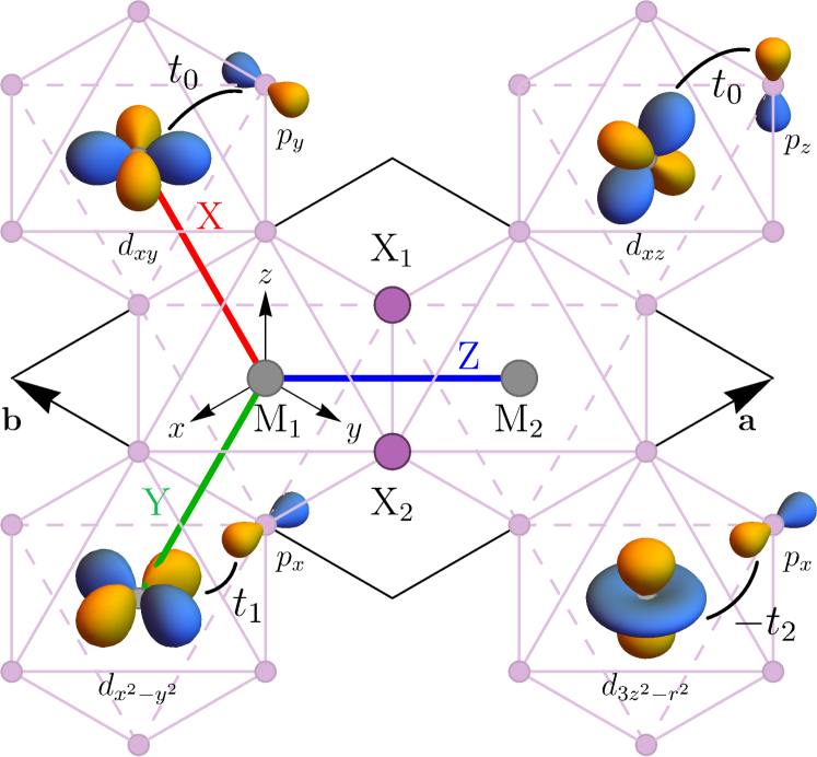
Figure 1: Edge-shared octahedra honeycomb structure unit cell $\mathbf{a,\ b}$, in global coordinates $xyz$. Transition metal sites M in gray and non-magnetic ligands X in purple. The n.n. bonds X, Y, Z are related by $C_{3}$ symmetry. The sites M₁, M₂, X₁, and X₂ are involved in the second order strong-coupling expansion on the Z bond. Indirect hopping integrals $t_{0}$, $t_{1}$ and $t_{2}$ are shown.

The on-site Hamiltonian of the M sites is described by the Kanamori interaction Kanamori (1963) as well as crystal field spitting:

$$H_{ee} = U\sum\limits_{\alpha}n_{\alpha\uparrow}n_{\alpha\downarrow}+\dfrac{U^{\prime}}{2}\sum\limits_{\begin{subarray}{c}\alpha\neq\beta,\\ \sigma,\sigma^{\prime}\end{subarray}}n_{\alpha\sigma}n_{\beta\sigma^{\prime}}$$ (1)

$$-\dfrac{J_{H}}{2}\sum\limits_{\begin{subarray}{c}\alpha\neq\beta,\\ \sigma,\sigma^{\prime}\end{subarray}}c^{\dagger}_{\alpha\sigma}c^{\dagger}_{\beta\sigma^{\prime}}c_{\beta\sigma}c_{\alpha\sigma^{\prime}}+J_{H}\sum\limits_{\alpha\neq\beta}c^{\dagger}_{\alpha\uparrow}c^{\dagger}_{\alpha\downarrow}c_{\beta\downarrow}c_{\beta\uparrow}$$

$$+\Delta_{c}\sum\limits_{\begin{subarray}{c}\alpha\in e_{\rm g},\\ \sigma\end{subarray}}c^{\dagger}_{\alpha\sigma}c_{\alpha\sigma},$$

where the density operator $n_{\alpha\sigma}$ is given by $c^{\dagger}_{\alpha\sigma}c_{\alpha\sigma}$, and $c^{\dagger}_{\alpha\sigma}$ is the creation operator with $\alpha$ orbital and spin $\sigma$. $U$ and $U^{\prime}$ are the intra-orbital and inter-orbital Hubbard interaction respectively, and $J_{H}$ is the Hund’s coupling for the spin-exchange and pair-hopping terms. $\Delta_{c}$ is a crystal field splitting on the M sites, originated from the surrounding octahedra, leading to the splitting of the $d$-orbitals into $t_{\rm 2g}$ and $e_{\rm g}$ orbitals. In a $d^{3}$ system one has half-filled $t_{\rm 2g}$ orbitals, where the Hund’s coupling $J_{H}$ selects for the S=3/2 configuration as the ground state, and the angular momentum is quenched. A table of the excited state energy spectrum is show in Appendix .1. The energies of the exited states are larger than the hopping integrals, which allows us to treat the tight binding hopping integrals as a perturbation.

In the edge shared octahedra structure, each bond between n.n. M sites involves two adjacent ligands, as shown in Fig. 1. A tight binding Hamiltonian between two transition metal sites M₁ and M₂ including the two adjacent ligands X₁ and X₂ is given below

$$H_{TB}=\left(\begin{array}[]{llll}\mathrm{0}_{5\times 5}&\mathbf{T_{M_{1}M_{2}}}&\mathbf{T_{M_{1}X_{1}}}&\mathbf{T_{M_{1}X_{2}}}\\ \mathbf{T_{M_{1}M_{2}}}^{\dagger}&\mathrm{0}_{5\times 5}&\mathbf{T_{M_{2}X_{1}}}&\mathbf{T_{M_{2}X_{2}}}\\ \mathbf{T_{M_{1}X_{1}}}^{\dagger}&\mathbf{T_{M_{2}X_{2}}}^{\dagger}&\mathrm{0}_{3\times 3}&\mathrm{0}_{3\times 3}\\ \mathbf{T_{M_{1}X_{2}}}^{\dagger}&\mathbf{T_{M_{2}X_{2}}}^{\dagger}&\mathrm{0}_{3\times 3}&\mathrm{0}_{3\times 3}\end{array}\right),$$ (2)

where $0_{n\times n}$ refers the $n\times n$ null matrix. The basis is chosen as $(C_{\mathrm{M}_{1},d}^{\dagger},C_{\mathrm{M}_{2},d}^{\dagger},C_{\mathrm{X}_{1},p}^{\dagger},C_{\mathrm{X}_{2},p}^{\dagger})$, where $C_{\mathrm{M}_{i},d}^{\dagger}=\left(c^{\dagger}_{i,x^{2}-y^{2}},c^{\dagger}_{i,3z^{2}-r^{2}},c^{\dagger}_{i,yz},c^{\dagger}_{i,xz},c^{\dagger}_{i,xy},\right)$ are five $d$-orbitals at site $\mathrm{M}_{i}$, and $C_{\mathrm{X}_{m},p}^{\dagger}=\left(c^{\dagger}_{m,p_{x}},c^{\dagger}_{m,p_{y}},c^{\dagger}_{m,p_{z}}\right)$ are three $p$-orbitals at ligand site $\mathrm{X}_{m}$. Each block of indirect hopping between $\mathrm{M}_{i}$ and $\mathrm{X}_{m}$ is denoted by $\mathbf{T_{M_{i}X_{m}}}$ and the direct hopping between $\mathrm{M}$ sites by $\mathbf{T_{M_{1}M_{2}}}$. The details of each block matrix will be presented latter.

To account for the indirect $d$ to $p$ hoppings we integrate out the $p$-orbitals through a perturbative procedure truncated at second order, leading to an effective $d$ to $d$ hopping model:

$$\mathbf{T^{\mathrm{eff}}_{M_{i}M_{j}}}=\sum_{(a,m)}\dfrac{\mathbf{T_{M_{i}X_{m}}}|a\rangle\langle a|\mathbf{T_{X_{m}M_{j}}}}{\Delta E_{a}},$$ (3)

where $(a,m)$ represent a sum over all single hole states $a$ of all sites X_m. The hole states are SOC states, thus creating two energy costs $\Delta E_{a}=\Delta-\lambda_{p}/2\text{ or }\Delta+\lambda_{p}$, where $\Delta=\epsilon_{d}-\epsilon_{p}$ is the atomic energy difference between M and X sites, and $\lambda_{p}$ is the SOC in $p$-orbitals. The SOC will introduce explicit spin dependence in the effective $d$ to $d$ hopping. The total effective hopping between the two M sites now reads

$$H^{\rm eff}_{TB}=\left(\begin{array}[]{llll}\mathrm{0}_{10\mathrm{x}10}&\mathbf{T_{M_{1}M_{2}}}+\mathbf{T^{\mathrm{eff}}_{M_{1}M_{2}}}\\ \mathbf{T_{M_{1}M_{2}}}^{\dagger}+\mathbf{T^{\mathrm{eff}}_{M_{1}M_{2}}}^{\dagger}&\mathrm{0}_{10\mathrm{x}10}\end{array}\right),$$ (4)

where we still retain the bare direct hoppings $\mathbf{T_{M_{1}M_{2}}}$. Below we focus on the ideal honeycomb structure and first examine the effects of $\mathbf{T^{\mathrm{eff}}_{M_{1}M_{2}}}$ before adding the direct hoppings $\mathbf{T_{M_{1}M_{2}}}$ and summarizing the resulting spin model.

III Ideal honeycomb structure

To understand the microscopic origin of the spin model, we start with the ideal honeycomb network surrounded by perfect edge shared octahedra. It was shown that the symmetry of the edge-shared octahedra Z bond allows Heisenberg $J$, Kitaev $K$, and symmetric off-diagonal $\Gamma$ interactions Rau et al. (2014); Yamaji et al. (2014); Katukuri et al. (2014). However, since their strengths depend on various exchange processes, we perform the strong coupling perturbation theory to determine the exchange terms.

Truncating at second order in perturbation theory, we arrive at the following Heisenberg-Kitaev $(J-K)$ spin model for the ideal honeycomb octahedra.

$$\begin{array}[]{c}H=\displaystyle\sum\limits_{\langle ij\rangle\in\gamma}J_{0}{\bf S}_{i}\cdot{\bf S}_{j}+K_{0}S_{i}^{\gamma}S_{j}^{\gamma},\\[11.38092pt] \end{array}$$ (5)

where $\gamma=x,y,z$ bond, and $J_{0}$ and $K_{0}$ refer to Heisenberg and Kitaev interactions for the ideal octahedra.

Below we present the details of the derivation of Heisenberg and Kitaev interactions. An explanation of the absence of the $\Gamma$ interaction within the second order perturbation theory is also discussed. The exchange processes include the contributions from both indirect and direct hoppings. We focus on the Z bond of the honeycomb Fig. 1, as the other two bonds are related by $C_{3}$ symmetry.

III.1 Superexchange path: indirect hopping

We first consider indirect hoppings between the M and X sites, which are the largest hopping integrals. They enter through the effective hoppings of Eq. (4). The non-zero indirect hopping between $\mathrm{M}_{1}$ and $\mathrm{X}_{1}$ sites $t_{0},\ t_{1},\ t_{2}$ are shown in Fig. 1. These hoppings are incorporated in $\mathbf{T^{eff}_{M_{1}M_{2}}}$, which can be simplified using the Slater-Koster decomposition and symmetry related $M-X$ bonds as shown in the Appendix. There are two contributions to both Heisenberg and Kitaev interactions, i.e., each interaction is composed of two exchange terms; one is from $t_{2g}-t_{2g}$ hoppings and the other is from $e_{\rm g}-t_{\rm 2g}$ hoppings

$$J_{0}=J_{0}^{\rm t_{2g}}+J_{0}^{\rm e_{g}},\ K_{0}=K_{0}^{\rm t_{2g}}+K_{0}^{\rm e_{g}},$$ (6)

where the superscript ${\rm t_{2g}}$ and ${\rm e_{g}}$ refer to its corresponding hopping processes. Below we present each exchange path leading to $J_{0}^{\rm t_{2g}}$, $K_{0}^{\rm t_{2g}}$, $J_{0}^{\rm e_{g}}$, and $K_{0}^{\rm e_{g}}$.

III.1.1 $t_{\rm 2g}-t_{\rm 2g}$ contributions

Introducing the effective hopping integral $t_{\mathrm{eff}}=\dfrac{t_{0}^{2}}{3}\left(\dfrac{2}{\Delta-\lambda_{p}/2}+\dfrac{1}{\Delta+\lambda_{p}}\right)$ between $M_{1}$ and $M_{2}$ via $p$-orbitals, and the ratio $r=\dfrac{2\lambda_{p}}{2\Delta+\lambda_{p}}$ between SOC $\lambda_{p}$ and the atomic energy difference $\Delta$, the hopping matrix involving only $t_{\rm 2g}$ orbitals, denoted by $t_{0}$ in Fig. 1, can be simplified in block form to

$$\mathbf{T^{eff}_{M_{1}M_{2}}}(t_{\rm 2g}\otimes t_{\rm 2g})=t_{\mathrm{eff}}\left(\begin{array}[]{rrr}0_{2\times 2}&\mathbf{\sigma}_{o}&i\dfrac{r}{2}\mathbf{\sigma}_{x}\\ \mathbf{\sigma}_{o}&0_{2\times 2}&-i\dfrac{r}{2}\mathbf{\sigma}_{y}\\ -i\dfrac{r}{2}\mathbf{\sigma}_{x}&i\dfrac{r}{2}\mathbf{\sigma}_{y}&0_{2\times 2}\end{array}\right),$$ (7)

where $t_{\rm 2g}=\{d_{yz},d_{xz},d_{xy}\}$ and $\sigma_{i}$ with $i=x,y,z$ are the Pauli matrices carrying the spin degrees of freedom and $\sigma_{o}$ is the $2\times 2$ identity matrix. The holes in the intermediate sates at the X site and their indirect hopping $\mathbf{T_{M_{i}X_{m}}}$ determine the type of $\sigma$ matrices in the effective hopping For example in the limit $\lambda_{p}\rightarrow 0$, only the $d_{yz}-d_{xz}$ term $t_{\mathrm{eff}}\sigma_{0}\rightarrow t^{2}_{0}/\Delta$ is present which contributes to the direct hopping channel. The new terms present for non-zero $\lambda_{p}$ are the spin-flip (SF) terms between $d_{yz}/d_{xz}$ and $d_{xy}$. Such terms would normally not appear in the second order perturbation process, as they involve a $d_{yz}/d_{xz}-p_{z}$ hopping followed by a $p_{x}/p_{y}-d_{xy}$ hopping, which will only occur if $p_{z}$ is entangled with $p_{x}/p_{y}$. The SOC among the $p_{x},p_{y},p_{z}$ generates such entanglement. Furthermore, when SOC is the dominant energy scale of the hole states, the wavefunctions are inevitably mixtures of $p$-orbitals and their spin, leading to $\sigma_{i}$ dependence proportional to the $r$ ratio of the SOC and atomic energy difference.

The superexchange process involving only $t_{\rm 2g}$ orbitals Eq. (7) result in

$$\begin{array}[]{c}J_{0}^{\rm t_{2g}}=\dfrac{8t^{2}_{\mathrm{eff}}}{9\left(U+2J_{H}\right)},\ K_{0}^{\rm t_{2g}}=-\dfrac{4(rt_{\mathrm{eff}})^{2}}{9\left(U+2J_{H}\right)}.\end{array}$$ (8)

The spin-dependent hoppings have generated a $S^{z}_{i}S^{z}_{j}$ Kitaev interaction. This can be rudimentarily understood by the following steps. To simplify the steps, we focus on one spin 1/2 electron hopping along the Z bond, through only a SF hopping. Imagining two sites starting in $(\uparrow,\uparrow)$ state, the SF hopping can lower the energy by the process: $(\uparrow,\uparrow)-\text{SF}-(0,\downarrow\uparrow)-\text{SF}-(\uparrow,\uparrow)$, at a energy cost of $-(rt_{\mathrm{eff}})^{2}/U$. On the other hand, if the two sites start in $(\uparrow,\downarrow)$ the SF process is forbidden from Pauli exclusion principle. Thus the exchange path starting from $(\uparrow,\uparrow)$ and ending in $(\uparrow,\uparrow)$ lowers the energy, which generates the FM $S^{z}_{i}S^{z}_{j}$ interaction. Carrying out the details for the S=3/2 leads to the expression of the spin exchange terms shown in Eq. (8).

Among the symmetry allowed terms, the symmetric off-diagonal term with operator $S^{x}_{i}S^{y}_{j}+S^{y}_{i}S^{x}_{j}=\dfrac{i}{2}\left(S_{i}^{-}S_{j}^{-}-S_{i}^{+}S_{j}^{+}\right)$ does not occur in the second order perturbation results. This operator would connect $(\uparrow,\uparrow)$ to $(\downarrow,\downarrow)$, which is definitely possible from a SF process, however, there is a subtle cancellation. Having a single Pauli matrix in the SF term creates such cancellation among the two paths within the spin block, resulting in a null $\Gamma$ term. Thus it becomes finite only when higher order perturbation terms are included, or when the octahedra are no longer ideal, as we will show in the later Sec. IV.

III.1.2 $e_{\rm g}-t_{\rm 2g}$ contributions

Given that the $p$-orbital’s hybridization with $e_{\rm g}$ is larger than with $t_{\rm 2g}$, denoted by $t_{1}$ and $t_{2}$ in Fig. 1,this contribution is essential. The final form of the effective $\mathbf{T^{\mathrm{eff}}_{M_{1}M_{2}}}(e_{\rm g}\otimes t_{\rm 2g})$ hopping includes SF terms in the $d_{yz},\ d_{xz}$ to $e_{\rm g}$ blocks, as well as spin-independent $-2t_{\rm eff}(t_{2}/t_{0})\sigma_{0}$ hopping between $d_{xy}$ and $d_{3z^{2}-r^{2}}$. The effective hopping matrix involving $e_{\rm g}-t_{\rm 2g}$ hoppings, in block matrix form, reads

$$\mathbf{T^{eff}_{M_{1}M_{2}}}(e_{\rm g}\otimes t_{\rm 2g})=t_{\mathrm{eff}}\left(\begin{array}[]{rrr}i\dfrac{r}{2}\dfrac{t_{1}}{t_{0}}\sigma_{y}&i\dfrac{r}{2}\dfrac{t_{1}}{t_{0}}\sigma_{x}&\lx@intercol\hfil 0_{2\times 2}\hfil\lx@intercol\\ -i\dfrac{r}{2}\dfrac{t_{2}}{t_{0}}\sigma_{y}&i\dfrac{r}{2}\dfrac{t_{2}}{t_{0}}\sigma_{x}&-2\dfrac{t_{2}}{t_{0}}\sigma_{o}\\ \end{array}\right),$$ (9)

where $e_{\rm g}=\{d_{x^{2}-y^{2}},d_{3z^{2}-r^{2}}\}$ and $t_{\rm 2g}=\{d_{yz},d_{xz},d_{xy}\}$. Carrying out the strong coupling expansion, these hoppings lead to the additional contribution to the Heisenberg and Kitaev interactions

$$\begin{array}[]{l}J_{0}^{\rm{e_{g}}}=-\dfrac{16\;J_{H}\;t_{\rm eff}^{2}}{3\left(\Delta_{c}+U^{\prime}-J_{H}\right)\left(\Delta_{c}+U^{\prime}+3J_{H}\right)}\dfrac{t_{2}^{2}}{t^{2}_{0}},\\ K_{0}^{\rm{e_{g}}}=\dfrac{2\;J_{H}(r\;t_{\rm eff})^{2}}{3\left(\Delta_{c}+U^{\prime}-J_{H}\right)\left(\Delta_{c}+U^{\prime}+3J_{H}\right)}\dfrac{t_{1}^{2}+t_{2}^{2}}{t^{2}_{0}}.\end{array}$$ (10)

Similar to the $t_{\rm 2g}-t_{\rm 2g}$ case, the SF terms contribute to the Kitaev interaction, while the spin-independent hopping, $-2t_{\rm eff}(t_{2}/t_{0})\sigma_{0}$, generates a FM Heisenberg term. The FM Heisenberg interaction originates from the competition of two exited states separated by Hund’s coupling, i.e, $e_{\rm g}$ paths consistent with the earlier findings obtained by the first principle calculations.Kashin et al. (2020); Soriano et al. (2020)

III.2 Direct hopping

The direct hopping, denoted by $t_{d1}$, $t_{d2}$, $t_{d3}$ and $\tilde{t}_{d0}$ in $\mathbf{T_{M_{1}M_{2}}}$ between M₁ and M₂ is given by

$$\begin{array}[]{l}\mathbf{T_{M_{1}M_{2}}}\left(t_{\rm 2g}\otimes t_{\rm 2g}\right)=\left(\begin{array}[]{ccccc}t_{d1}&t_{d2}&0\\ t_{d2}&t_{d1}&0\\ 0&0&t_{d3}\\ \end{array}\right)\otimes\mathbf{\sigma}_{o},\\[19.91684pt] \mathbf{T_{M_{1}M_{2}}}\left(e_{\rm g}\otimes t_{\rm 2g}\right)=\left(\begin{array}[]{ccc}0&0&0\\ 0&0&\tilde{t}_{d0}\\ \end{array}\right)\otimes\mathbf{\sigma}_{o}.\end{array}$$ (11)

The Slater-Koster decomposition is explained in the Appendix. Since there is no SF hopping terms, this does not generate the Kitaev interaction, but changes the Heisenberg interaction.

III.3 Summary and Comments

Combining both indirect and direct hopping contributions, the two exchange interactions for the ideal octahedra environment Eq. (5) are found to be

$$J_{0} = \dfrac{4\left(2t_{d1}^{2}+2(t_{\rm eff}+t_{d2})^{2}+t_{d3}^{2}\right)}{9\left(U+2J_{H}\right)}$$

$$- \dfrac{4J_{H}\left(2t_{\rm eff}(t_{2}/t_{0})-{\tilde{t}}_{d0}\right)^{2}}{3\left(\Delta_{c}+U^{\prime}-J_{H}\right)\left(\Delta_{c}+U^{\prime}+3J_{H}\right)},$$

$$K_{0} = -\dfrac{4\;(r\;t_{\rm eff})^{2}}{9\left(U+2J_{H}\right)}$$ (12)

$$+ \dfrac{2\;J_{H}(r\;t_{\rm eff})^{2}}{3\left(\Delta_{c}+U^{\prime}-J_{H}\right)\left(\Delta_{c}+U^{\prime}+3J_{H}\right)}\dfrac{t_{1}^{2}+t_{2}^{2}}{t^{2}_{0}}.$$

Thus for the ideal honeycomb structure, the $J-K$ model is derived within the second order perturbation theory.

Some comments are useful, which will also motivate further investigation on the effects of trigonal distortion presented in the next section. Kitaev and Heisenberg interactions have been generated while the $\Gamma$ interaction has not appeared at second order due to a subtle cancellation. The Kitaev has been generated purely from SF hoppings and has a prefactor of $r^{2}=(2\lambda_{p}/(2\Delta+\lambda_{p}))^{2}$, while the Heisenberg includes spin-independent hopping contributions. Nevertheless both $K$ and $J$ have two contributions which come with opposite signs: one from $t_{2g}$ only paths and the other from the paths involving $e_{\rm g}$. This leads to a smaller Kitaev compared to Heisenberg interaction, unless the contribution from $e_{\rm g}$ paths reduces the overall strength of the Heisenberg interaction. So long as the crystal field spitting is not excessively large, the naturally larger $e_{\rm g}$ hoppings will drive the system to a FM Heisenberg interaction.

The FM $J-K$ model pins the moment along the cubic axis when the quantum fluctuations are taken into accountJackeli and Avella (2015); Chaloupka and Khaliullin (2016), not along the observed [111] direction in CrI₃. We thus investigate if other interaction terms may be generated. The $\Gamma$ interaction allowed by the symmetry can be finite if higher order perturbation terms are included. However, one may ask if there are other interactions allowed by a slight distortion of the lattice within the second order perturbation theory without invoking higher order terms. Indeed TMT materials do not have ideal octahedra, but have either rhombohedral $R\bar{3}$ or monoclinic $C2/m$ structures, and their magnetism strongly depends on structural differences and number of layers.Klein et al. (2018); Song et al. (2018); Klein et al. (2019); Kim et al. (2019b) Below we study the effects of distorted octahedra, which induce additional hopping integrals which were forbidden without the distortion.

IV Effects of distortion: distorted octahdera

CrI₃ goes through a structural transition from $C2/m$ to $R{\bar{3}}$ structure at low temperature.McGuire et al. (2015) In the rhombohedral structure, there are two types of X ligand position deviations from the ideal octahedra structure. As shown in Fig. 2(a), a single octahedron can be viewed as two shaded triangles. One distortion is the staggered rotations of the two triangles denoted by $\delta x$ blue arrows, with displacements of X sites perpendicular to the $\hat{c}=[1,1,1]/\sqrt{3}$ direction. The other distortion is the compression of the distance between these two triangles along the $\hat{c}$-axis denoted by $\delta x^{\prime}$ orange arrows, with displacements along the $\hat{c}$ direction. Here the dimensionless parameters $\delta x$ and $\delta x^{\prime}$ are in units of the distance between the n.n. M sites $d_{M}$. Analytic formulas of the new positions of X sites under staggered rotations and compression are found in Appendix .3. In the $R\bar{3}$ space group there are other types of distortions, namely the M${}_{1}-$X_2,4,6 bond length can be different from the M${}_{1}-$X_1,3,5 bond length. This type of distortion is generally exceedingly small compared to $\delta x$ and $\delta x^{\prime}$ and we neglect it in the following analysis. Fig. 2(b) shows a top view of the the honeycomb unit cell with two such distorted octahedra forming the Z bond, and the staggered rotation of the right octahedron is the mirror image of the left octahedron.

\begin{overpic}[width=390.25534pt]{z_bond_distortion_representation_TAPANTA_v6.pdf} \put(1.0,95.0){a)} \put(1.0,40.0){b)} \end{overpic}

Figure 2: a) The distorted octahedra in $R{\bar{3}}$ is shown. The octahedron made of X ligand can be viewed as two yellow triangles normal to the $\hat{c}=[1,1,1]/\sqrt{3}$ direction. The blue arrows represent new positions of X due to the staggered rotations of the two yellow triangular faces. The change of position X due to the staggered rotations is parameterized by $\delta x$. In addition, there is a compression of the two yellow triangles, squeezed as shown by the orange arrows parallel to the $\hat{c}$-axis. The change of position due to the compression is parameterized by $\delta x^{\prime}$. b) A top view of distortions in a unit cell is shown. The dotted circles $\odot$ indicate the new position of X moving out of the page along +$\hat{c}$ while the circled cross $\otimes$ indicate a new position of X moving into the page toward $-\hat{c}$. The exact positions of X_{(1,2,3,4,5,6)} as a function of $\delta x$, $\delta x^{\prime}$ are found in the Appendix.

The distortion-induced hopping matrices have all elements non-zero in $\mathbf{T_{M_{i}X_{m}}}$ as a result of lowering the local symmetry of the octahedron from $O_{h}$ to $D_{3}$. We denote the new distortion allowed hopping integrals as $\delta t_{i}$. Starting with the distortion-induced hoppings, we follow the procedure described in Sec. III, namely we use the distortion-induced $\mathbf{T_{M_{i}X_{m}}}$ matrices to derive the effective $\mathbf{T^{\mathrm{eff}}_{M_{1}M_{2}}}(t_{\rm 2g}\otimes t_{\rm 2g})$ and $\mathbf{T^{\mathrm{eff}}_{M_{1}M_{2}}}(e_{\rm g}\otimes t_{\rm 2g})$. Details of their form is deferred to Appendix .4. Treating the distortion-induced effective hoppings as a perturbation against the on-site interactions Eq. (1) the minimal n.n. spin model is finally given by

$$\begin{array}[]{l}H=\displaystyle\sum\limits_{\langle ij\rangle\in\alpha\beta(\gamma)}\Big{[}J{\bf S}_{i}\cdot{\bf S}_{j}+KS_{i}^{\gamma}S_{j}^{\gamma}+\Gamma(S_{i}^{\alpha}S_{j}^{\beta}+S_{i}^{\beta}S_{j}^{\alpha})\\ \ \ \ \ \ \ \ \ \ \ \ \ \ \ \ \ \ +\ \Gamma^{\prime}(S_{i}^{\alpha}S_{j}^{\gamma}+S_{i}^{\beta}S_{j}^{\gamma}+S_{i}^{\gamma}S_{j}^{\alpha}+S_{i}^{\gamma}S_{j}^{\beta})\Big{]}\\ \ \ \ \ \ \ \ \ +\displaystyle\sum_{i}A_{c}({\bf S}_{i}\cdot\mathbf{\hat{c}})^{2},\end{array}$$ (13)

where $\alpha,\beta,(\gamma)$ refers to the $\gamma$ bond taking $\alpha$ and $\beta$ spin components Rau et al. (2014); Rau and Kee , and $\mathbf{\hat{c}}=[1,1,1]/\sqrt{3}$. In addition to the $J-K$ terms, two symmetric off-diagonal terms $\Gamma$ and $\Gamma^{\prime}$ have been generated, as well as the single-ion term $A_{c}$ allowed by the $C_{3}$ symmetry present on every site. $\Gamma$, $\Gamma^{\prime}$ and $A_{c}$ are proportional to distortion induced hoppings $\delta t$ as well as $r$, thus both distortion-induced hoppings and SOC is needed to bring rise to these terms. The form of the spin model $J-K-\Gamma-\Gamma^{\prime}-A_{c}$ to leading order in ${\delta t_{i}}$ as well as $e_{\rm g}$ contributions are listed in Table 6 in the Appendix. Note that both Heisenberg and Kitaev interactions are renormalized by the distortion, but the Heisenberg interaction has a linear term in $\delta t$, while Kitaev interaction does not.

V Application to CrI₃

To apply the above model to understand the magnetism in CrI₃, we use ab initio calculations to obtain the microscopic parameters. The calculation is performed with Vienna ab initio simulation package (VASP)Kresse and Hafner (1993). We use the Perdew-Burke-Ernzerhof (PBE) functionalPerdew et al. (1997) in our calculations. The experimental bulk structureMcGuire et al. (2015) is used for the calculations. We use WANNIER90Mostofi et al. (2008) to extract the hopping integrals.

From the density functional theory results, we estimate the crystal field splitting $\Delta_{c}=1253$ meV from on-site Cr $d$-orbitals as well as a crystal field splitting from the on-site I $p$-orbitals of $\Delta_{p}=528$ meV. From Cr $d$- and I $p$- orbitals we extract the atomic energy difference between Cr and I $\Delta=2070$ meV. Finally we find the dominant indirect $p-d$ hopping integrals $t_{0}$, $t_{1}$ and $t_{2}$ and the direct $d-d$ hoppings parameters, listed in Table 1, as well as the distortion induced $p-d$ hoppings, listed in Table 2. We verified that $t_{0}$, $t_{1}$ and $t_{2}$ obtained by the ab initio calculation match well with the Slater-Koster expectations of Eq. (A.4).

$t_{0}$	$t_{1}$	$t_{2}$	$t_{d1}$	$t_{d2}$	$t_{d3}$	$\tilde{t}_{d0}$
590.1	-992.13	-558.3	44.67	-41.26	-147.44	-20.75

Table 1: Indirect and direct hoppings in units of meV obtained by ab initio calculations. The hopping integrals are defined in Eq. (LABEL:eq:indirect) and Eq. (11).

$\delta t_{1}$	$\delta t_{2}$	$\delta t_{3}$	$\delta t_{4}$	$\delta t_{5}$	$\delta t_{1}^{\prime}$	$\delta t_{2}^{\prime}$	$\delta t_{3}^{\prime}$	$\delta t_{4}^{\prime}$
2.34	21.76	-22.81	-61.74	65.86	70.97	-43.50	-49.41	29.65

Table 2: Distortion-induced indirect hoppings in units of meV obtained by ab initio calculations. The hopping integrals are defined in Eq. (A.20).

In the ab initio calculations, we find a sizable crystal field spitting $\Delta_{p}$ on the ligand I sites, which we have not taken into account in the earlier analysis. It is about $528$  meV, which is comparable to an estimated SOC parameter of $\lambda_{p}=630$ meV. To capture its effects we revisit the effective hopping derivation, and add the crystal field spitting $\Delta_{p}$ on the X sites. Then the energy level in Eq. (3) split into three levels as $\Delta E_{a}=\Delta-\frac{\lambda}{2},\Delta+\frac{1}{4}\left(2\Delta_{p}+\lambda\pm\sqrt{\left(2\Delta_{p}-\lambda\right)^{2}+8\lambda^{2}}\right)$. While the holes in I sites are no longer pure total angular momentum states, the SOC is sizable enough to carry the spin entanglement through to the spin model. We found that second order perturbation theory, including the spitting $\Delta_{p}$ in the effective hoppings, does not change the form of the spin model Eq. (13). The analytic formulas would be vastly more complex in this case, so we proceed to a direct numerical evaluation of $J-K-\Gamma-\Gamma^{\prime}-A_{c}$ exchange terms using effective hoppings $\mathbf{T^{eff}_{M_{1}M_{2}}}$ obtained by the ab-inito calculations listed in the Tables.

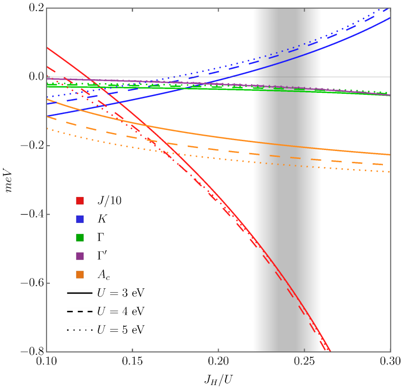
Figure 3: Spin model parameters $J$, $K$, $\Gamma$, $\Gamma^{\prime}$, and $A_{c}$ estimated from ab initio parameters and plotted against $J_{H}/U$. Solid, dashed, and dotted lines correspond to $U=3{\rm eV},\ 4{\rm eV}\text{ and }5{\rm eV}$ respectively. Shaded region corresponds to $J_{H}/U\sim 0.24$ which is relevant to CrI₃ microscopics.

Assuming the spherical symmetry, i.e., $U^{\prime}=U-2J_{H}$, we are left with two unknown parameters $U$ and $J_{H}$. We plot $J$, $K$, $\Gamma$, $\Gamma^{\prime}$, and $A_{c}$ as a function of $J_{H}/U$ for several $U$ values, with results shown in Fig. 3. The dominant term is Heisenberg except near the range $0.11\lesssim J_{H}/U\lesssim 0.13$ where $J$ is almost zero before it changes the sign. The sign of $J(K)$ are sensitive to the ratio $J_{H}/U$ and an adequately large Hund’s coupling allows the FM Heisenberg (AFM Kitaev) interaction to persevere. This reflects the competition of the $t_{\rm 2g}$ vs $e_{\rm g}$ terms seen in Eq. (III.3), with $e_{\rm g}$ eventually wining over $t_{\rm 2g}$ leading to the FM Heisenberg interaction. The distortion induced $\Gamma-\Gamma^{\prime}-A_{c}$ come in with FM sign, and the single-ion anisotropy $A_{c}$ is the sizable term. Adopting the ratio of $J_{H}/U\sim 0.24$ obtained by cRPA clculations Jang et al. (2019), CrI₃ sits in the shaded area in Fig. 3. CrI₃ is a ferromagnet with non-negligible $K-\Gamma-\Gamma^{\prime}-A_{c}$, and we now examine the implication of these exchange terms on the observed moment.

\begin{overpic}[width=390.25534pt]{several_moments_v2.pdf} \put(1.0,38.0){a)} \put(34.0,38.0){b)} \put(67.666,38.0){c)} \end{overpic}

Figure 4: Moment pinning calculation for difrent values of $(J,K,\Gamma)$ in the ferromagnetic phase: a) $(-1.00,-0.20,\ 0.00)$, b) $(-0.20,-1.00,\ 0.00)$, c) $(-0.20,-1.00,-0.02)$. Kitaev interaction always prefers the cubic axis in panel a) and b). A small interaction like $\Gamma$ is necessary to pin along the $\hat{c}$ direction as show in panel c).

VI Magnetic Anisotropy

We have shown how the ideal honeycomb structure leads to $J-K$ model up to second order in perturbation, while distortions additionally generate $\Gamma-\Gamma^{\prime}-A_{c}$. The magnetic moment of the ferromagnetic state obtained with the FM $J-K$ model is pinned along the cubic axis such as $[100]$ and $C_{3}$ equivalent directions via quantum fluctuationsJackeli and Avella (2015); Chaloupka and Khaliullin (2016). We take a closer look at the effects of $\Gamma-\Gamma^{\prime}-A_{c}$ on the moment direction. We show three examples in Fig. 4 to illustrate the moment pinning direction.

Following the method in Ref. [59], we perform exact diagonalization calculations on an eight site honeycomb cluster, with the cluster setup shown in the Appendix. Once the ground state wavefunction $\left|GS\right\rangle$ is obtained, the probability distribution $P=\left|\left\langle\Psi_{FM}(\theta,\phi)\right|\left.GS\right\rangle\right|^{2}$ is computed, where $\left|\Psi_{FM}(\theta,\phi)\right\rangle$ is a ferromagnetic ansatz with moment direction pointing at $(\theta,\phi)$ on the sphere. Results are show in Fig. 4 for different values of $J$, $K$, and $\Gamma$. Independent of ratio of $J$ and $K$, the moment is along the cubic axis as shown in the panel (a) and (b). On the other hand, when a small FM $\Gamma$ is introduced, the moment is along the $\hat{c}$ direction as shown in panel (c). This effect can be anticipated from the classical analysis. The classical $J-K-\Gamma$ model in the FM state with moment $\mathbf{S}_{0}=(S^{x}_{0},S^{y}_{0},S^{z}_{0})$ has an energy density per unit cell $u^{c}=(3J+K)+2\Gamma(S^{x}_{0}S^{y}_{0}+S^{y}_{0}S^{z}_{0}+S^{z}_{0}S^{x}_{0})$, which demands $min\left[u^{c}\right]\Rightarrow min\left[sgn(\Gamma)(S^{x}_{0}S^{y}_{0}+S^{y}_{0}S^{z}_{0}+S^{z}_{0}S^{x}_{0})\right]$. When $\Gamma<0$ we have $min\left[-(S^{x}_{0}S^{y}_{0}+S^{y}_{0}S^{z}_{0}+S^{z}_{0}S^{x}_{0})\right]\Rightarrow\mathbf{S}_{0}=\hat{c}$ leading to a moment pined on the [1,1,1]. We choose $\Gamma/K\ll 1$ to show that a tiny FM $\Gamma$ anisotropy results in the ${\hat{c}}$-axis moment shown in Fig. 4 (c).

FM $\Gamma^{\prime}$ has the identical effect as FM $\Gamma$ with respect to the moment direction of the ferromagnet. Clearly FM $A_{c}$ also promotes the ${\hat{c}}$-axis moment direction. All three interactions individually prefer the moment on the ${\hat{c}}$-axis. This effect is bigger than the quantum fluctuation effect of cubic axis pinning from the Kitaev term resulting in the observed ${\hat{c}}$-axis moment direction.

VII Spin gap and finite transition temperature

The preceding results suggest that it is likely that CrI₃ has dominant FM Heisenberg and smaller Kitaev interaction, and the magnetic anistoropy originates from the distortion of the octahedra together with the SOC of heavy ligands. The magnetic ordering pattern changes from bulk to films Huang et al. (2017); Sivadas et al. (2018); Jiang et al. (2019); Jang et al. (2019); Kim et al. (2019b); Soriano et al. (2019), suggesting a strong coupling between magnetism and crystal structures, which further implies the importance of the distorted octahedra in the presence of SOC. Our microscopic model has an interesting connection to the previous studies. The Kitaev and single-ion anistoropy in addition to the Heisenberg interaction were found in Ref.Xu et al. (2018) using density functional theory. If $\Gamma=\Gamma^{\prime}$, the $J-\Gamma-\Gamma^{\prime}$ model maps to the XXZ modelLado and Fernández-Rossier (2017); Kim et al. (2019a) in the $a-b-c$ crystallographic coordinate

$$J{\bf S}_{i}\cdot{\bf S}_{j} +\Gamma(S_{i}^{x}S_{j}^{y}+S_{i}^{y}S_{j}^{x}+S_{i}^{x}S_{j}^{z}+S_{i}^{z}S_{j}^{x}+S_{i}^{y}S_{j}^{z}+S_{i}^{z}S_{j}^{y})$$ (14)

$$\Longrightarrow\;\;\;J_{ab}{\bf S}_{i}\cdot{\bf S}_{j}+J_{c}S^{c}_{i}S^{c}_{j},$$

where $J_{ab}=J-\Gamma$ and $J_{c}=3\Gamma$.

Since the exchange parameters strongly depend on $J_{H}/U$, $\Delta_{c}/U$, and tight binding parameters, it is useful to obtain experimental inputs to determine some parameters. The inelastic neutron scattering experiments and magneto-Raman spectroscopy have reported a spin gap of approximately 0.36 meV at the Brillouin zone (BZ) center $\Gamma$-point.Chen et al. (2018); Cenker et al. (2021) This is also consistent with a small anistoropy found in the ferromagnetic resonance experimentLee et al. (2020), which is about $0.07$ meV leading to the spin gap of 0.3 meV.

Based on our spin wave analysis using the $J-K-\Gamma-\Gamma^{\prime}-A_{c}$ model including the second n.n. DM interaction, the spin wave dispersion $\omega_{\bf k}$ is expressed as $\omega_{0}+\rho\;k^{2}$ around the $\Gamma$-point. Here $\omega_{0}$ and $\rho$ are the spin gap and stiffness, respectively, and they are given by

$$\begin{gathered}\omega_{o}=-S(3\Gamma+6\Gamma^{\prime}+2A_{c}),\\ \rho=\dfrac{S}{12}\left|3J+K-\Gamma-2\Gamma^{\prime}-\tfrac{(K+2\Gamma-2\Gamma^{\prime})^{2}}{2\left(2\Gamma+4\Gamma^{\prime}+2A_{c}+3J+K\right)}\right|\end{gathered}$$ (15)

The details of the linear spin wave theory (LSWT) is presented in Appendix .7.

Kitaev and DM interactions do not generate a gap at the $\Gamma$-point within the LSWT. The classical ferromagnetic ground state under the Kitaev and DM terms have a continuous degeneracy, and as a result expanding around this ground state in the LSWT will not result in a spin gap from these terms. The spin gap is rather small, as expected because it is originated from a combination of slightly distorted octahedra and SOC, i.e., $\Gamma$, $\Gamma^{\prime}{}$, and $A_{c}$. While small, it is essential for a finite $T_{c}$ in a single layer CrI₃. In the FM ordered phase, at low temperatures the magnons are excited and their number is given by $N_{s}(T)=\int d^{2}k\frac{1}{e^{\beta\omega_{\bf k}}-1}=\frac{\pi}{\beta\rho}\int_{\beta\omega_{0}}\frac{dx}{e^{x}-1}.$ Without the spin gap $\omega_{0}$, $N_{s}$ diverges in two-dimension at any temperature except $T=0$, i.e., the celebrated Mermin-Wagner theoremMermin and Wagner (1966). Thus one can understand the essential role of $\omega_{0}$ which cuts the divergence, and allows the FM ordering at finite temperatures, as long as $\omega_{0}(T)$ remains finite for $T\leq T_{c}$. While quantifying the transition temperature requires further analysis Maksimov and Chernyshev (2020) , the temperature dependence of $\rho(T)$ and $\omega_{0}(T)$ from the inelastic neutron scattering measurementChen et al. (2018) indicates the crucial role of $\omega_{0}(T)$ which vanishes at $T_{c}$.

Another important parameter is the Kitaev interaction $K$, which leads to a gap at the the BZ corner $K$-point known as the Dirac gapLee et al. (2020), reported in the neutron scattering.Chen et al. (2018, 2020) However, the second n.n. DM term also generates the Dirac gap.Chen et al. (2018, 2020) We would like to point out that $\Gamma$ and $\Gamma^{\prime}$ also play a part in the Dirac gap as shown in Eq. (A.38). Estimating the Kitaev interaction by an independent experimental measurement and further analysis on the individual role of the Kitaev and DM interactions remain to be resolved in future studies.

VIII Summary and Discussion

We have shown a microscopic derivation of the n.n. spin model for honeycomb Mott insulators with three electrons in $t_{\rm 2g}$ orbitals at M sites surrounded by octahedral cages of ligands X with strong SOC. Using the standard strong-coupling perturbation theory, we found that there are only Heisenberg and Kitaev interactions for the ideal honeycomb lattice among the three symmetry allowed interactions ($J,K,\Gamma$), because $\Gamma$ is zero up to the second order perturbation. The exchange paths between $t_{\rm 2g}$ and $t_{\rm 2g}$ vs. $t_{\rm 2g}$ and $e_{\rm g}$ via ligands generate opposite signs for both Heisenberg and Kitaev interactions. The Heisenberg interaction is of order $t_{\rm eff}^{2}/U$, while the Kitaev is smaller by a factor of $r^{2}\sim(\lambda_{p}/\Delta)^{2}$. The FM Heisenberg interaction originates from the $e_{\rm g}$ paths, with the hopping integral between $e_{\rm g}$ and $p$-orbitals being larger compared to $t_{\rm 2g}$ and $p$-orbitals.

The FM Heisenberg and Kitaev interaction leads to FM ordering, but the moment direction is pinned along the cubic $x$, $y$, or $z$ axis, e.g., [100] (and $C_{3}$ equivalent directions) via quantum fluctuations. The $\hat{c}$-axis, [111], moment pinning found in CrI₃ should thus originate from other interactions, which are also responsible for the spin gap at the $\Gamma$-point in the neutron scattering measurementChen et al. (2018). Including the distorted octahedra present in the rhombohedral structure, three additional spin interactions are found. Inspecting the linear order in the distortion-induced hopping paths within the second order perturbation theory, $\Gamma$, $\Gamma^{\prime}$ and single-ion anisotropy $A_{c}$ contain terms linear in the distortion-induced hopping integrals. The Heisenberg interaction also contains such additional linear term, but the Kitaev does not, implying that it is possible to fine-tune a system closer to the Kitaev dominant regime via trigonal distortions.

In this work we have focused on the nature of the monolayer, however, some comments are in place when considering the physics of the bulk. We showed that the $t_{\rm 2g}-t_{\rm 2g}$ vs. $e_{\rm g}-t_{\rm 2g}$ contributions to the intra-layer Heisenberg term $J$ are opposite in sign. This property should hold for inter-layer Heisenberg interaction $J_{\perp}$ as well, because it is determined from superexchange processes. Thus the magnetic ordering pattern between layers depends on the details of orbital compositions. From the ab initio calculation, we found that the inter-layer hopping ranges from 10meV to 30meV. This leads to $J_{\perp}$ of order 0.1 meV. While it does not affect the intra-layer magnetism presented here, it is important for the ordering pattern in the bulkHuang et al. (2017); Sivadas et al. (2018); Jiang et al. (2019); Jang et al. (2019); Kim et al. (2019b); Soriano et al. (2019).

Comparison to $J_{\rm eff}=1/2$, S=1, and 3/2 spin systems would be useful. The SOC is necessary to generate the bond-dependent interaction, as spin and orbitals should be entangled to get such a directional dependent spin interaction. However, the presence of SOC is not enough to find an exotic phase like a spin liquid, because the dominant interaction is often the Heisenberg interaction. To compare different spin cases, a summary of the ideal honeycomb exchange interactions, $J_{0}$, $K_{0}$, and $\Gamma_{0}$ including the effective indirect hopping ($t_{\rm eff})$ and direct hopping ($t_{d}$) integrals, only up to the second order perturbation, is shown in the following Table 3.

Spin	Heisenberg $J_{0}$	Kitaev $K_{0}$	symm. [-0.1cm] off-diagonal $\Gamma_{0}$
$J_{\rm eff}=1/2\;(d^{5})$	$O(\frac{t_{d}^{2}}{t_{\rm eff}^{2}})$	$O(\frac{J_{H}}{U})$	$O(\frac{t_{d}}{t_{\rm eff}}\frac{J_{H}}{U})$
$S=1\;(d^{8})$	$O(r^{2})$	$O(r^{2})$	0
$S=3/2\;(d^{3})$	$O(1)$	$O(r^{2})$	0

Table 3: The leading term of the exchange interactions for the ideal honeycomb structure in unit of $t_{\rm eff}^{2}/U$ for different spin $S$ including only up to the second order perturbation terms. See the Appendix for the full expression of $JK\Gamma\Gamma^{\prime}A_{c}$ for S=3/2 including the trigonal distortion-induced hopping contributions.

Focusing on the ideal octahedra and n.n. model via second order superexchange processes, $J_{\rm eff}=1/2$ is unique because the Heisenberg term is absent. On the other hand, for the S=1 model from $d^{2}$ in $e_{\rm g}$-orbitals, the heavy ligand SOC generates the Kitaev interaction, which has the same order of magnitude with $J$. In fact, $K=-2J$, if only $e_{\rm g}$ paths are considered.Stavropoulos et al. (2019) For S=3/2 case, we found that $J$ is order 1 in units of roughly $t_{\rm eff}^{2}/U$, while $K$ is smaller by $r^{2}$. Thus it is hard to compete with the Heisenberg interaction. We speculate that this is valid for spins equal or higher than 3/2. Unlike S=1/2 and S=1 cases, the Heisenberg interaction is dominant in S=3/2, but a delicate cancellation among different contributions to the Heisenberg interaction, may let the Kitaev interaction overtake a major place. In particular, the Heisenberg interaction is more sensitive to the distortion-induced hopping integrals than the Kitaev term as shown in Table 6 in the Appendix, manipulating ocathedra may be a way to tune the system to a desired Kitaev dominant regime.

In summary, in the ideal octahedra environment, we find that there are only two spin interactions, Heisenberg and Kitaev interactions. Kitaev interaction is generally weaker compared to the Heisenberg interaction in contrast to the lower spin models. Indirect hoppings among $t_{\rm 2g}$ and $t_{\rm 2g}$ vs. $e_{\rm g}$ and $t_{\rm 2g}$ have opposite contributions. A detailed balance between the two indirect and direct hopping contributions highly depends on the hopping integrals, Hund’s coupling strength, and crystal field spitting. $\Gamma$ interaction is absent up to the second order due to a subtle cancellation. We further show that trigonal distortion allows three additional interactions, two symmetric off-diagonal interactions $\Gamma$ and $\Gamma^{\prime}$, and single-ion anisotropy $A_{c}$ along the $\hat{c}$-axis. They are all linearly proportional to a distortion-induced hopping integral. While they are much smaller than the Heisenberg interaction, they are essential for a spin gap in the FM phase of CrI₃ leading to a finite $T_{c}$. Our study offers a microscopic route to the n.n. spin models, $J-K-\Gamma-\Gamma^{\prime}{}-A_{c}$ interactions. Given that there are five exchange terms within the n.n. model, and second n.n. interactions including DM may be comparable to $\Gamma$, $\Gamma^{\prime}$ and $A_{c}$, further theoretical and experimental studies are required to determine the microscopic parameters of CrI₃ beyond the n.n. model.

-¿

*

APPENDIX

.1 Energy levels of on-site Kanamori Hamiltonian

To obtain the n.n. spin interaction, we used the second order perturbation theory, where the dominant interaction is Eq. (1). First we note that in the lowest energy state there are three electrons at each metal site M. The exchange processes then involve one electron hopping between M sites. Thus the intermediate states have two electrons in $t_{\rm 2g}$-orbitals on one M site and four electrons in either $t_{\rm 2g}$- or $e_{\rm g}$-orbitals on the other M site. On the other hand the single-ion anisotropy would follow from a single M site, where the three electrons in the ground state interact with an exited three electron state. The energy levels of all states involved in these exchange processes are given in Table 4.

Degen.	Energy	Microscopics
2 electrons (only in $t_{2g}$)
1	$E_{A,2,1}$	$=U+2J_{H}+2\epsilon_{d}$
2	$E_{A,2,2}$	$=U-\ J_{H}+2\epsilon_{d}$
3	$E_{A,2,3}$	$=U^{\prime}+\ J_{H}+2\epsilon_{d}$
9	$E_{A,2,4}$	$=U^{\prime}-\ J_{H}+2\epsilon_{d}$
3 electrons (GS)
4	$E_{A,3,gs}$	$=3U^{\prime}-3J_{H}+3\epsilon_{d}$
3 electrons (only in $t_{2g}$)
4	$E_{A,3,1}$	$=3U^{\prime}+3\epsilon_{d}$
6	$E_{A,3,2}$	$=U+2U^{\prime}-2J_{H}+3\epsilon_{d}$
6	$E_{A,3,3}$	$=U+2U^{\prime}+3\epsilon_{d}$
3 electrons (2-$t_{2g}$, 1-$e_{g}$)
8	$E_{A,3,e1}$	$=U+2U^{\prime}-2J_{H}+\Delta_{c}+3\epsilon_{d}$
4	$E_{A,3,e2}$	$=U+2U^{\prime}+J_{H}+\Delta_{c}+3\epsilon_{d}$
24	$E_{A,3,e3}$	$=3U^{\prime}-3J_{H}+\Delta_{c}+3\epsilon_{d}$
24	$E_{A,3,e4}$	$=3U^{\prime}+\Delta_{c}+3\epsilon_{d}$
4 electrons (only in $t_{2g}$)
1	$E_{A,4,1}$	$=2U+4U^{\prime}+4\epsilon_{d}$
2	$E_{A,4,2}$	$=2U+4U^{\prime}-3J_{H}+4\epsilon_{d}$
3	$E_{A,4,3}$	$=\ U+5U^{\prime}-\ J_{H}+4\epsilon_{d}$
9	$E_{A,4,4}$	$=\ U+5U^{\prime}-3J_{H}+4\epsilon_{d}$
4 electrons (3-$t_{2g}$, 1-$e_{g}$)
4	$E_{A,4,e1}$	$=6U^{\prime}+\Delta_{c}+4\epsilon_{d}$
6	$E_{A,4,e2}$	$=U+5U^{\prime}+\Delta_{c}+4\epsilon_{d}$
10	$E_{A,4,e3}$	$=6U^{\prime}-6J_{H}+\Delta_{c}+4\epsilon_{d}$
18	$E_{A,4,e4}$	$=U+5U^{\prime}-4J_{H}+\Delta_{c}+4\epsilon_{d}$
18	$E_{A,4,e5}$	$=6U^{\prime}-2J_{H}+\Delta_{c}+4\epsilon_{d}$
24	$E_{A,4,e6}$	$=U+5U^{\prime}-2J_{H}+\Delta_{c}+4\epsilon_{d}$

Table 4: Spectrum of Hamiltonian Eq. (1). Listed states can contribute to the second order strong coupling perturbation.

.2 Ideal hoppings

In the ideal octahedron environment the allowed indirect hoppings are show in Fig. 5. On the M${}_{1}-$X₁ bond we have the hopping matrix

$$\begin{array}[]{cccc}&&\begin{array}[]{ccc}p_{x}&p_{y}&p_{z}\end{array}&\\[5.69046pt] \mathbf{T_{M_{1}X_{1}}}&=&\left(\begin{array}[]{ccc}t_{1}&0&0\\ -t_{2}&0&0\\ 0&0&0\\ 0&0&t_{0}\\ 0&t_{0}&0\end{array}\right)&\begin{array}[]{l}d_{x^{2}-y^{2}}\\ d_{3z^{2}-r^{2}}\\ d_{yz}\\ d_{xz}\\ d_{xy}\ \ \ \ \ \ ,\end{array}\end{array}$$ (A.1)

The other indirect bonds $\mathbf{T_{M_{2}X_{2}}},\ \mathbf{T_{M_{2}X_{1}}},\ \mathbf{T_{M_{1}X_{2}}}$ are obtained from $\mathbf{T_{M_{1}X_{2}}}$ by consecutively applying the symmetry operation of the octahedron $C_{4}(0,0,1)$. Use of Eq. (LABEL:eq:indirect) and symmetry related bonds are then used in Eq. (4) to arrive at effective hoppings Eq. (7) and Eq. (9). Slater-Koster analysisSlater and Koster (1954) allows us to decompose $t_{0},\ t_{1},\ t_{2}$ and $t_{3}$ into $\sigma$- and $\pi$-bonding integrals between $d$- and $p$-orbitals

$$\begin{array}[]{llll}t_{0}=t_{pd\pi},&t_{1}=\dfrac{\sqrt{3}t_{pd\sigma}}{2},&t_{2}=\dfrac{t_{pd\sigma}}{2},&t_{3}=t_{pd\sigma},\\[8.5359pt] \lx@intercol\hfil t_{pd\sigma}<0,\ t_{pd\pi}>0,\ \left\lvert t_{pd\pi}\right\lvert<\left\lvert t_{pd\sigma}\right\lvert.\hfil\lx@intercol\end{array}$$ (A.4)

The direct hoppings Eq. (11) include $\delta$-bonding in addition to $\sigma$- and $\pi$-bondings

$$\begin{array}[]{cc}t_{d1}=\dfrac{t_{dd\pi}+t_{dd\delta}}{2},&t_{d2}=\dfrac{-t_{dd\pi}+t_{dd\delta}}{2}\\ t_{d3}=\dfrac{3t_{dd\sigma}+t_{dd\delta}}{4},&\tilde{t}_{d0}=\dfrac{\sqrt{3}\left(t_{dd\sigma}-t_{dd\delta}\right)}{4},\\[8.5359pt] \lx@intercol\hfil t_{dd\sigma}<0,\ t_{dd\pi}>0,t_{dd\delta}<0,\hfil\lx@intercol\\ \lx@intercol\hfil\left\lvert t_{dd\delta}\right\lvert<\left\lvert t_{dd\pi}\right\lvert<\left\lvert t_{dd\sigma}\right\lvert,\hfil\lx@intercol\\[8.5359pt] \end{array}$$ (A.9)

with the Anderse prediction $t_{dd\sigma}:t_{dd\pi}:t_{dd\delta}=-6:4:-1$.

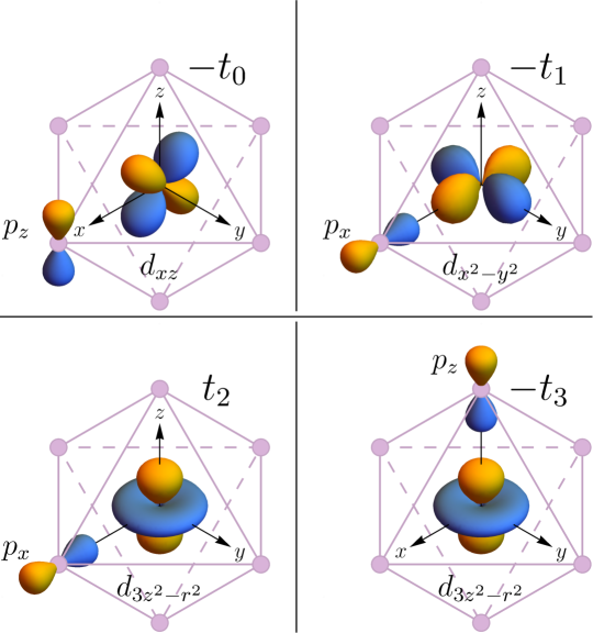
Figure 5: Indirect hoppings from X site to M site, in the global coordinates $xyz$.

.3 Positions of X sites under distortions

In the $R{\bar{3}}$ space group, octahedra made of two triangles as shown in Fig. 2 are rotated around ${\hat{c}}$-axis denoted by $\delta x$ blue arrows. Furthermore there is a slight change in the distance between these two triangles denoted by $\delta x^{\prime}$ yellow arrows. The new positions of ligands are parameterized by dimensionless $\delta x$ and $\delta x^{\prime}$, in units of the distance $d_{M}$ between M₁ and M₂. One can track the positions $\mathbf{r}_{m}$ of X_m, as it is related to the undistorted position $\mathbf{r}_{o,m}$, $\delta x$ and $\delta x^{\prime}$:

$$\begin{array}[]{l}\mathbf{r}_{m}=\mathbf{r}_{o,m}+\delta x\ d_{M}(\xi^{a}_{m}\ \hat{\mathbf{a}}+\xi^{b}_{m}\ \hat{\mathbf{b}})+\delta x^{\prime}\ d_{M}\zeta_{m}\ \hat{\mathbf{c}}\\[5.69046pt] \begin{array}[]{c|rrrrrrrrrrrrrr}m&\lx@intercol\hfil\mathbf{r}_{o,m}\hfil\lx@intercol&&\lx@intercol\hfil\left(\xi^{a}_{m},\xi^{b}_{m}\right)\hfil\lx@intercol&&\zeta_{m}\\ \hline\cr X_{1}&(&\frac{-d_{M}}{\sqrt{2}}&0&0&)&&(&-1&,&-1&)&&1\\ X_{2}&(&0&\frac{d_{M}}{\sqrt{2}}&0&)&&(&1&,&1&)&&-1\\ X_{3}&(&0&\frac{-d_{M}}{\sqrt{2}}&0&)&&(&1&,&0&)&&1\\ X_{4}&(&0&0&\frac{d_{M}}{\sqrt{2}}&)&&(&-1&,&0&)&&-1\\ X_{5}&(&0&0&\frac{-d_{M}}{\sqrt{2}}&)&&(&0&,&1&)&&1\\ X_{6}&(&\frac{d_{M}}{\sqrt{2}}&0&0&)&&(&0&,&-1&)&&-1\\ \end{array},\end{array}$$ (A.19)

where X_m lable sites as in Fig. 2(a) and $\hat{\mathbf{a}}$, $\hat{\mathbf{b}}$ and $\hat{\mathbf{c}}$ are unit vectors along the lattice vectors of Fig. 2(b).

.4 Distortion-induced hoppings

To get the distortion-induced hoppings one needs to find the directional cosines of the indirect $d-p$ bonds using the ligand positions Eq. (A.19). With the metal site located at $\mathbf{r}_{\mathrm{M}_{1}}$ and ligand X_m located at $\mathbf{r}_{m}$, the required directional cosines follow from $\mathbf{r}_{m}-\mathbf{r}_{\mathrm{M}_{1}}$. They are the inputs in the Slater-Koster formula for rotated bonds Ref. [75]. Here we only show the leading term in each matrix element generated from the above procedure. Note that all elements become finite, and the distortion-induced hopping between $t_{\rm 2g}$ and $p$-oribtials are denoted by $\delta t_{i}$ and $e_{\rm g}$ and $p$-orbitals by $\delta t^{\prime}_{i}$:

$$\mathbf{T_{M_{1}X_{1}}}=\left(\begin{array}[]{ccc}t_{1}&\delta t^{\prime}_{1}&\delta t^{\prime}_{2}\\ -t_{2}&\delta t^{\prime}_{3}&\delta t^{\prime}_{4}\\ \delta t_{1}&\delta t_{2}&\delta t_{3}\\ \delta t_{4}&\delta t_{1}&t_{0}\\ \delta t_{5}&t_{0}&\delta t_{1}\\ \end{array}\right),$$ (A.20)

where X₁ labels the site as in Fig. 2(a). The distorted octahedron realizes the $D_{3}$ point group, which contains $C_{3}(1,1,1)$ and $C_{2}^{\prime}(-1,1,0)$ rotations. The hoppings $\mathbf{T_{M_{1}X_{3}}}$ and $\mathbf{T_{M_{1}X_{5}}}$ are recovered by applying $C_{3}(1,1,1)$ to $\mathbf{T_{M_{1}X_{1}}}$. Further $\mathbf{T_{M_{1}X_{1}}}$ relates to $\mathbf{T_{M_{1}X_{2}}}$ by a $C_{2}^{\prime}(-1,1,0)$. Finally $\mathbf{T_{M_{1}X_{2}}}$ relates to $\mathbf{T_{M_{1}X_{4}}}$ and $\mathbf{T_{M_{1}X_{6}}}$ by $C_{3}(1,1,1)$. The direct hopping integrals denoted by $\mathbf{T_{M_{1}M_{2}}}$ is same the as Eq. (11). Making use of Eq. (A.20) we derive effective hoppings $\mathbf{T^{\mathrm{eff}}_{M_{1}M_{2}}}$ following the method in the main text Eq. (4). The distortion induced effective hoppings to leading order in $\delta t$ and listed in Table 5.

Table 5: Effective hoppings to leading order in distortion-induced hoppings, where $\delta t$ are defined in Eq. (A.20). Distortion induced hoppings are grouped in: $\delta t_{a}=\delta t_{1}-\delta t_{4},\ \delta t_{b}=2\delta t_{1}+\delta t_{4},\ \delta t_{c}=\delta t_{3}+\delta t_{5},\ \delta t_{d}=\delta t_{1}-\delta t_{2},\ \delta t_{e}=\delta t_{1}+\delta t_{4},\ \delta t_{f}=\delta t_{1}+\delta t_{2}$.

$\mathbf{T^{\mathrm{eff}}_{M_{1}M_{2}}}(t_{\rm 2g}\otimes t_{\rm 2g})=t_{\rm eff}\left(\begin{array}[]{ccc}T_{A}&T_{C}&T_{D}\\ T_{C}^{\dagger}&T_{A}&\ UT_{D}U^{\dagger}\\ T_{D}^{\dagger}&U^{\dagger}T_{D}^{\dagger}U&T_{B}\end{array}\right)$	$\mathbf{T^{\mathrm{eff}}_{M_{1}M_{2}}}(e_{\rm g}\otimes t_{\rm 2g})=t_{\rm eff}\left(\begin{array}[]{ccl}\tilde{T}_{A}&-U\tilde{T}_{A}U^{\dagger}&\tilde{T}_{C}\\ \tilde{T}_{B}&\ \ U\tilde{T}_{B}U^{\dagger}&\tilde{T}_{D}\\ \end{array}\right)$
$U=\mathrm{e}^{i\pi\frac{1}{\sqrt{2}}\left(\frac{\sigma_{x}}{2}-\frac{\sigma_{y}}{2}\right)}=\dfrac{i}{\sqrt{2}}(\sigma_{x}-\sigma_{y})$
$\begin{array}[]{ccl}T_{A}&=&\left(2\dfrac{\delta t_{3}}{t_{0}}+\dfrac{t_{d1}}{t_{\rm eff}}\right)\sigma_{o}\\[8.5359pt] T_{B}&=&\left(4\dfrac{\delta t_{5}}{t_{0}}+\dfrac{t_{d3}}{t_{\rm eff}}\right)\sigma_{o}\\[8.5359pt] T_{C}&=&\left(1+\dfrac{t_{d2}}{t_{\rm eff}}\right)\sigma_{o}+i\dfrac{r}{2}\dfrac{\delta t_{a}}{t_{0}}\left(\sigma_{x}+\sigma_{y}\right)\\[8.5359pt] T_{D}&=&\dfrac{\delta t_{b}}{t_{0}}\sigma_{o}+i\dfrac{r}{2}\left(\sigma_{x}-\dfrac{\delta t_{c}}{t_{0}}\sigma_{y}-\dfrac{\delta t_{d}}{t_{0}}\sigma_{z}\right)\\[8.5359pt] \end{array}$	$\begin{array}[]{ccl}\tilde{T}_{A}&=&\left(\dfrac{\delta t^{\prime}_{2}}{t_{0}}+\dfrac{\delta t_{d}t_{1}}{t_{0}^{2}}\right)\sigma_{o}+i\dfrac{r}{2}\left(\left(\dfrac{\delta t_{3}t_{1}}{t_{0}^{2}}-\dfrac{\delta t^{\prime}_{1}}{t_{0}}\right)\sigma_{x}+\dfrac{t_{1}}{t_{0}}\sigma_{y}-\dfrac{\delta t_{e}t_{1}}{t_{0}^{2}}\sigma_{z}\right)\\[8.5359pt] \tilde{T}_{B}&=&\left(\dfrac{\delta t^{\prime}_{4}}{t_{0}}-\dfrac{\delta t_{f}t_{2}}{t_{0}^{2}}\right)\sigma_{o}+i\dfrac{r}{2}\left(\left(\dfrac{\delta t_{3}t_{2}}{t_{0}^{2}}-\dfrac{\delta t^{\prime}_{3}}{t_{0}}\right)\sigma_{x}-\dfrac{t_{2}}{t_{0}}\sigma_{y}-\dfrac{\delta t_{a}t_{2}}{t_{0}^{2}}\sigma_{z}\right)\\[8.5359pt] \tilde{T}_{C}&=&i\dfrac{r}{2}\left(\left(\dfrac{\delta t_{1}t_{1}}{t_{0}^{2}}-\dfrac{\delta t_{2}^{\prime}}{t_{0}}\right)\left(\sigma_{x}+\sigma_{y}\right)-2\left(\dfrac{\delta t_{5}t_{1}}{t_{0}^{2}}-\dfrac{\delta t_{1}^{\prime}}{t_{0}}\right)\sigma_{z}\right)\\[8.5359pt] \tilde{T}_{D}&=&\left(-2\dfrac{t_{2}}{t_{0}}+\dfrac{\tilde{t}_{d0}}{t_{\rm eff}}\right)\sigma_{o}+i\dfrac{r}{2}\left(\dfrac{\delta t_{1}t_{2}}{t_{0}^{2}}+\dfrac{\delta t_{4}^{\prime}}{t_{0}}\right)\left(\sigma_{x}-\sigma_{y}\right).\end{array}$

Table 6: Spin model terms, under distortions, to leading order in $\delta t$. Distortion-induced $\delta t$ defined in Eq. (A.20), and character subscripted $\delta t$ defined in caption of Table 5 and Eq. (A.32)

		$t_{\rm 2g}\otimes t_{\rm 2g}$		$e_{\rm g}\otimes t_{\rm 2g}$
$J$	$=$	$\dfrac{4\left(2t_{d1}^{2}+2(t_{\rm eff}+t_{d2})^{2}+t_{d3}^{2}\right)}{9\left(U+2J_{H}\right)}$		$-\dfrac{4J_{H}\left(2t_{\rm eff}(t_{2}/t_{0})-{\tilde{t}}_{d0}\right)^{2}}{3\left(\Delta_{c}+U^{\prime}-J_{H}\right)\left(\Delta_{c}+U^{\prime}+3J_{H}\right)}$
		$+\dfrac{32t_{\rm eff}}{9(U+2J_{H})}\left(t_{d1}\dfrac{\delta t_{3}}{t_{0}}+t_{d3}\dfrac{\delta t_{5}}{t_{0}}\right)$
$K$	$=$	$-\dfrac{4\;(r\;t_{\rm eff})^{2}}{9\left(U+2J_{H}\right)}$		$\dfrac{2\;J_{H}(r\;t_{\rm eff})^{2}}{3\left(\Delta_{c}+U^{\prime}-J_{H}\right)\left(\Delta_{c}+U^{\prime}+3J_{H}\right)}\dfrac{t_{1}^{2}+t_{2}^{2}}{t^{2}_{0}}$
$\Gamma$	=	$-\dfrac{8(rt_{\rm eff})^{2}}{9\left(U+2J_{H}\right)}\left(\dfrac{\delta t_{c}}{t_{0}}\right)$		$-\dfrac{4J_{H}(rt_{\rm eff})^{2}}{3\left(\Delta_{c}+U^{\prime}-J_{H}\right)\left(\Delta_{c}+U^{\prime}+3J_{H}\right)}\left(\dfrac{t_{1}(t_{1}\delta t_{3}-t_{0}\delta t^{\prime}_{1})}{t_{0}^{3}}-\dfrac{t_{2}(t_{2}\delta t_{3}-t_{0}\delta t^{\prime}_{3})}{t_{0}^{3}}\right)$
$\Gamma^{\prime}$	=	$-\dfrac{4(rt_{\rm eff})^{2}}{9\left(U+2J_{H}\right)}\left(\dfrac{\delta t_{d}}{t_{0}}\right)$		$-\dfrac{2J_{H}(rt_{\rm eff})^{2}}{3\left(\Delta_{c}+U^{\prime}-J_{H}\right)\left(\Delta_{c}+U^{\prime}+3J_{H}\right)}\left(-\dfrac{t_{1}^{2}\delta t_{e}}{t_{0}^{3}}+\dfrac{t_{2}^{2}\delta t_{a}}{t_{0}^{3}}\right)$
$A_{c}$	=	$-\dfrac{4(rt_{\rm eff})^{2}}{\left(U+3J_{H}-U^{\prime}\right)}\left(\dfrac{\delta t_{\alpha}}{t_{0}}\right)$		$-\dfrac{4J_{H}(rt_{\rm eff})^{2}}{\Delta_{c}\left(\Delta_{c}+3J_{H}\right)}\left(\dfrac{t_{1}}{t_{0}}\left(\dfrac{\delta t_{\beta}t_{1}}{t_{0}^{2}}+\dfrac{\delta t^{\prime}_{\alpha}}{t_{0}}\right)-\dfrac{t_{2}+t_{3}}{t_{0}}\left(\dfrac{\delta t_{\beta}t_{2}+2\delta t_{1}t_{3}}{t_{0}^{2}}+\dfrac{\delta t^{\prime}_{\beta}}{t_{0}}\right)\right)$

.5 Single-ion anisotropy term

Due to the distortion and SOC, the single-ion anisotropic term is also generated via the hopping to anions which can hop back to create spin-dependent on-site terms denoted by $\mathbf{T^{\rm eff}_{M_{1}M_{1}}}=\mathbf{T^{\rm eff}_{M_{2}M_{2}}}$. Without the trigonal distortion, the effective hopping integrals between $t_{\rm 2g}$ at M₁ are given by

$$\begin{array}[]{l}\mathbf{T_{M_{1}M_{1}}^{\mathrm{eff}}}(t_{2g}\otimes t_{2g})=\\ t_{\mathrm{eff}}\left(\begin{array}[]{rrr}4\sigma_{o}&ir\sigma_{z}&-ir\sigma_{y}\\ -ir\sigma_{z}&4\sigma_{o}&ir\sigma_{x}\\ ir\sigma_{y}&-ir\sigma_{x}&4\sigma_{o}\\ \end{array}\right).\end{array}$$ (A.26)

Similarly, effective hopping between $t_{2g}$ and $e_{g}$ is found as

$$\begin{array}[]{l}\mathbf{T_{M_{1}M_{1}}^{\mathrm{eff}}}(e_{g}\otimes t_{2g})=\\ t_{\mathrm{eff}}\left(\begin{array}[]{rrr}ir\dfrac{t_{1}}{t_{0}}\sigma_{x}&ir\dfrac{t_{1}}{t_{0}}\sigma_{y}&-i2r\dfrac{t_{1}}{t_{0}}\sigma_{z}\\ ir\dfrac{t_{2}+t_{3}}{t_{0}}\sigma_{x}&-ir\dfrac{t_{2}+t_{3}}{t_{0}}\sigma_{y}&\lx@intercol\hfil 0_{2\times 2}\hfil\lx@intercol\\ \end{array}\right).\end{array}$$ (A.31)

They lead to an ${\bf S}_{i}\cdot{\bf S}_{i}$ term, which is just equal to $S(S+1)$, an irrelevant constant to the spin model. Thus there is no single-ion anisotropy without the trigonal distortion. With the trigonal distortion, the single-ion anisotropy along $\hat{c}$-axis is generated:

$$\begin{array}[]{ccl}A_{c}&=&-\dfrac{4(rt_{\rm eff})^{2}}{\left(U+3J_{H}-U^{\prime}\right)}\left(\dfrac{\delta t_{\alpha}}{t_{0}}\right)\\[11.38092pt] &&-\dfrac{4J_{H}(rt_{\rm eff})^{2}}{\Delta_{c}\left(\Delta_{c}+3J_{H}\right)}\left(\dfrac{t_{1}}{t_{0}}\left(\dfrac{\delta t_{\beta}t_{1}}{t_{0}^{2}}+\dfrac{\delta t^{\prime}_{\alpha}}{t_{0}}\right)\right.\\[11.38092pt] &&\left.-\dfrac{t_{2}+t_{3}}{t_{0}}\left(\dfrac{\delta t_{\beta}t_{2}+2\delta t_{1}t_{3}}{t_{0}^{2}}+\dfrac{\delta t^{\prime}_{\beta}}{t_{0}}\right)\right),\end{array}$$ (A.32)

where $\delta t_{\alpha}=-2\delta t_{1}+\delta t_{2}+\delta t_{3}+\delta t_{4}+\delta t_{5}$, $\delta t_{\beta}=\delta t_{2}+\delta t_{3}$, $\delta t^{\prime}_{\alpha}=-\delta t_{1}^{\prime}+\dfrac{\sqrt{3}\delta t_{4}^{\prime}-\delta t_{2}^{\prime}}{2}$, and $\delta t^{\prime}_{\beta}=-\delta t_{3}^{\prime}+\dfrac{\sqrt{3}\delta t_{2}^{\prime}+\delta t_{4}^{\prime}}{2}$.

.6 Spin interaction with trigonal distortion

Putting them all together, we have Heisenberg, Kitaev, $\Gamma$, $\Gamma^{\prime}$, and single-ion anisotropy $A_{c}$ term. Their form to leading order in distortion induced hoppings $\delta t$ are summarized in Table 6 bellow. Note that the Kitaev interaction does not have any linear term of distortion, and $\Gamma$, $\Gamma^{\prime}$ and single-ion anisotropy $A_{c}$ along $\hat{c}$-axis are finite due to both SOC and distortion.

.7 Spin Wave Theory

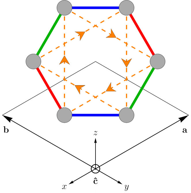
Figure 6: X Y and Z bonds of the $J-K-\Gamma-\Gamma^{\prime}-A_{c}$ shown in red, green and blue respectively. Second n.n are shown in orange. The orange arrows indicate when $\mathrm{sgn}(ij)=+1$ in the DM term.

We consider the $J-K-\Gamma-\Gamma^{\prime}-A_{c}$ as well as the second n.n. DM term ($\mathbf{D_{c}}$)

$$\begin{array}[]{lcl}H&=&\displaystyle\sum\limits_{\begin{subarray}{c}\langle i,j\rangle\in\alpha\beta(\gamma)\end{subarray}}\Big{[}J\mathbf{S}_{i}\cdot\mathbf{S}_{j}+KS_{i}^{\gamma}S_{j}^{\gamma}+\Gamma\left(S_{i}^{\alpha}S_{j}^{\beta}+S_{i}^{\beta}S_{j}^{\alpha}\right)\\ &&\ \ \ \ \ \ \ \ \ \ \ \ \ \ \ +\Gamma^{\prime}\left(S_{i}^{\alpha}S_{j}^{\gamma}+S_{i}^{\beta}S_{j}^{\gamma}+S_{i}^{\gamma}S_{j}^{\alpha}+S_{i}^{\gamma}S_{j}^{\beta}\right)\Big{]}\\[8.5359pt] &&+\displaystyle\sum\limits_{\langle\langle i,j\rangle\rangle}\mathbf{D_{c}}\cdot\left(\mathbf{S}_{i}\times\mathbf{S}_{j}\right)+\displaystyle\sum\limits_{i}A_{c}\left(\mathbf{S}_{i}\cdot\mathbf{\hat{c}}\right)^{2},\end{array}$$ (A.33)

where $\mathbf{D_{c}}=D_{c}\ \mathrm{sgn}(ij)\hat{c}$ and $\mathrm{sgn}(ij)=+1$ when $i$ to $j$ points along the orange arrows in Fig. 6. The standard Holstein-Primakoff transformation Holstein and Primakoff (1940) expanded to linear order in $S$ read

$$\begin{array}[]{lllll}S^{+}&=&\sqrt{2S}\left(1-\dfrac{a^{\dagger}a}{2S}\right)^{\frac{1}{2}}a&\simeq&\sqrt{2S}a,\\[8.5359pt] \ S^{-}&=&\sqrt{2S}a^{\dagger}\left(1-\dfrac{a^{\dagger}a}{2S}\right)^{\frac{1}{2}}&\simeq&\sqrt{2S}a^{\dagger},\\[8.5359pt] \ S^{z}&=&S-a^{\dagger}a.\end{array}$$ (A.34)

Using the above and Fourier transforming Eq. (A.33) leads to

$$\begin{array}[]{c}H=E_{CL}+\sum\limits_{\mathbf{k}\in BZ}\mathrm{x}_{\mathbf{k}}^{\dagger}\mathbf{h_{k}}\mathrm{x}_{\mathbf{k}},\\[8.5359pt] \mathrm{x}_{\mathbf{k}}^{\dagger}=(a^{\dagger}_{\mathbf{k}},\ b^{\dagger}_{\mathbf{k}},\ a_{\mathbf{-k}},\ b_{\mathbf{-k}}),\\[14.22636pt] \mathbf{h_{k}}=\left(\begin{array}[]{cccc}h_{o-}(\mathbf{k})&h_{1}(\mathbf{k})&0&h_{2}(\mathbf{k})\\ h_{1}(\mathbf{k})^{*}&h_{o+}(\mathbf{k})&h_{2}(-\mathbf{k})&0\\ 0&h_{2}(-\mathbf{k})^{*}&h_{o+}(\mathbf{k})&h_{1}(\mathbf{k})\\ h_{2}(\mathbf{k})^{*}&0&h_{1}(\mathbf{k})^{*}&h_{o-}(\mathbf{k})\end{array}\right),\end{array}$$ (A.35)

where the two species of bosons $a_{\mathbf{k}}$ and $b_{\mathbf{k}}$ correspond to the two sublattices of the unit cell. The $h(\mathbf{k})$ terms are

$$\begin{array}[]{l}h_{o\pm}(\mathbf{k})=h_{o}\pm h_{DM}(\mathbf{k}),\\[5.69046pt] h_{o}=-S\left(2A_{c}+2\Gamma+4\Gamma^{\prime}+3J+K\right),\\[5.69046pt] h_{DM}(\mathbf{k})=2SD_{c}\left(\sin({\bf a\cdot k})+\sin({\bf b\cdot k})\right.\\ \ \ \ \ \ \ \ \ \ \ \ \ \ \ \ \ \ \ \ \ \ \ \ \ \ \ \ \ \ \ \ \ \ \ \ \ \left.-\sin({\bf(a+b)\cdot k})\right),\\[5.69046pt] h_{1}(\mathbf{k})=-\dfrac{S\left(\Gamma+2\Gamma^{\prime}-3J-K\right)}{3}(1+\mathrm{e}^{-i\mathbf{a}\cdot\mathbf{k}}+\mathrm{e}^{i\mathbf{b}\cdot\mathbf{k}}),\\[5.69046pt] h_{2}(\mathbf{k})=\dfrac{S\left(2\Gamma-2\Gamma^{\prime}+K\right)}{6}\left((1-i\sqrt{3})\mathrm{e}^{-i\mathbf{a}\cdot\mathbf{k}}\right.\\ \ \ \ \ \ \ \ \ \ \ \ \ \ \ \ \ \ \ \ \ \ \ \ \ \ \ \ \ \ \ \ \ \ \ \left.+(1+i\sqrt{3})\mathrm{e}^{i\mathbf{b}\cdot\mathbf{k}}-2\right),\end{array}$$ (A.36)

where $\mathbf{a}$ and $\mathbf{b}$ are the lattice vectors in Fig. 6. Following standard methods of diagonalizing BdG HamiltoniansColpa (1978) we find the lowest eigenvalue around the $\Gamma$ point in the BZ, and upon expanding to orders of $k$, we get the spin gap $\omega_{o}$ and spin stiffness $\rho$:

$$\begin{array}[]{l}\omega_{\mathbf{k}}=\omega_{o}+\rho k^{2}\\[11.38092pt] \omega_{o}=S\left|3\Gamma+6\Gamma^{\prime}+2A_{c}\right|\\[11.38092pt] \lx@intercol\rho=\dfrac{S}{12}\Bigg{|}3J+K-\Gamma-2\Gamma^{\prime}\hfil\lx@intercol\\ \lx@intercol\hfil\ \ \ \ \ \ \ \ \ \ \ \ \ -\dfrac{(K+2\Gamma-2\Gamma^{\prime})^{2}}{2\left(2\Gamma+4\Gamma^{\prime}+2A_{c}+3J+K\right)}\Bigg{|}.\lx@intercol\end{array}$$ (A.37)

At the K point in the BZ the Dirac gap is $\omega^{K}_{+}-\omega^{K}_{-}$ where

$$\begin{array}[]{ccl}\omega^{K}_{+}&=&S\Big{\{}\left(6\Gamma^{\prime}+2A_{c}+3J\right)\left(4\Gamma+2\Gamma^{\prime}+2A_{c}+3J+2K\right)\\ &&+6\sqrt{3}D_{c}\left(2\Gamma+4\Gamma^{\prime}+2A_{c}+3J+K\right)+27D_{c}^{2}\Big{\}}^{1/2},\\[11.38092pt] \omega^{K}_{-}&=&S\left|2\Gamma+4\Gamma^{\prime}+2A_{c}+3J+K-3\sqrt{3}D_{c}\right|.\end{array}$$ (A.38)

.8 Exact diagonalization calculations

The moment pinning calculations are carried out by finding the ground state from exact diagonalization on an 8 site ($2\text{x}2$) honeycomb cluster with periodic conditions, shown in Fig. 7.

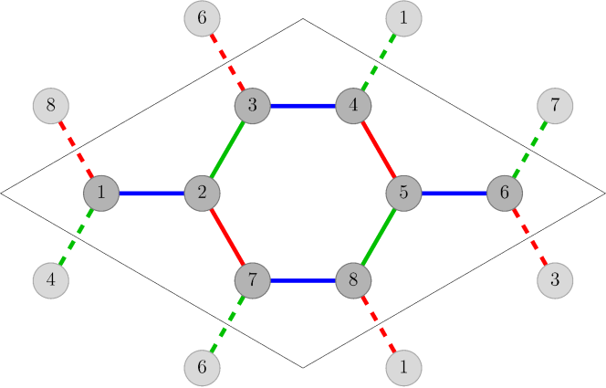
Figure 7: X,Y and Z bonds show in red, green and blue respectively. Dashed bonds represent the periodic boundary conditions.