Flux mobility delocalization in the Kitaev spin ladder

Abstract

We study the Kitaev spin-$1/2$ ladder, a model which exhibits self-localization due to fractionalization caused by exchange frustration. When a weak magnetic field is applied, the model is described by an effective fermionic Hamiltonian, with an additional time reversal symmetry breaking term. We show that this term alone is not capable of delocalizing the system but flux mobility is a prerequisite. For magnetic fields larger but comparable to the flux gap, fluxes become mobile and drive the system into a delocalized regime, featuring finite dc transport coefficients. Our findings are based on numerical techniques, exact diagonalization and dynamical quantum typicality, from which, we present results for the specific heat, the dynamical energy current correlation function, as well as the inverse participation ratio, contrasting the spin against the fermion representation. Implications of our results for two-dimensional extensions of the model will be speculated on.

¶Introduction.

Quantum spin liquids (QSL) are intriguing states of strongly correlated and highly entangled magnetic moments lacking spontaneous symmetry breaking and finite local order parameters down to zero temperature $T=0K$ Savary and Balents (2017); Zhou et al. (2017); Knolle and Moessner (2019). Instead, they feature topological order parameters and fractional excitations. One renown example of a $\mathbb{Z}_{2}$ QSL is the exactly solvable, two-dimensional (2D), Kitaev, spin-$1/2$ model (KSM), on a Honeycomb lattice Kitaev (2006); Hermanns et al. (2018). The spins that reside on the vertices of the Honeycomb lattice exhibit frustrating compass interactions and as a result fractionalize into fermions and $\mathbb{Z}_{2}$ gauge fluxes. Hence the total Hilbert space is fragmented in subspaces with reduced or absent translation symmetry. While the ground state resides in a uniform flux sector, fluxes can be thermally excited, thus becoming a temperature activated binary disorder for the fermions to scatter off.

Besides the original 2D-KSM, variants of it with different spin Stavropoulos et al. (2019); Baskaran et al. (2008); Rousochatzakis et al. (2018) or dimensionality have also been discussed in the literature Motome and Nasu (2020); Feng et al. (2007); Wu (2012); Steinigeweg and Brenig (2016); Metavitsiadis and Brenig (2017); Metavitsiadis et al. (2019); Agrapidis et al. (2019). The Kitaev ladder, a one-dimensional (1D) KSM is a very interesting model because the reduced dimensionality inflicts additional peculiarities upon it. The fermionic representation with the emergent $\mathbb{Z}_{2}$ gauge field still holds but in 1D the scattering off of fermions on disorder leads to localization Metavitsiadis and Brenig (2017). Thus in the 1D-KSM, single particle states are Anderson localized Anderson (1958) effectively leading to many body localization (MBL) Nandkishore and Huse (2015); Alet and Laflorencie (2018). The paradigm of localization in the absence of external disorder goes back to two-constituent systems (light-heavy particles) Kagan and Maksimov (1984) and has currently resurfaced in fracton phases of matter Nandkishore and Hermele (2019) with numerous applications on lattice gauge models and more De Roeck and Huveneers (2014); Schiulaz et al. (2015); Yao et al. (2016); Smith et al. (2017); Mondaini and Cai (2017); Michailidis et al. (2018); Mamaev et al. (2019); Brenes et al. (2018); Yarloo et al. (2019); Sala et al. (2020).

While transition metal compounds with a Kramers doublet due to strong spin-orbit coupling are good candidates for realizing the KSM Jackeli and Khaliullin (2009); Chaloupka et al. (2010); Takagi et al. (2019), a proximate Kitaev-QSL is the closest that has been reported so far Plumb et al. (2014); Nussinov and van den Brink (2015); Banerjee et al. (2016); Choi et al. (2012); Nishimoto et al. (2016); Yadav et al. (2016); Kitagawa et al. (2018); Wulferding et al. (2020). A valuable alternative for realizing the KSM might occur in cold atom experiments where compass interactions can be engineered Duan et al. (2003). Furthermore, optical lattices are also advancing the experimental study of non-ergodic systems exhibiting MBL Schreiber et al. (2015). Remarkably, the demonstration for realizing lattice gauge model with $\mathbb{Z}_{2}$ gauge fields coupled to 1D fermions has recently been reported Barbiero et al. (2019). Thus, all three fascinating fields of Kitaev-QSL, MBL, and lattice gauge models that will be discussed in this work, share the prospect of experimental materialization.

Here, we present results on the 1D-KSM including a uniform external magnetic field. First, using the specific heat we show that fluxes have a clear imprint to the specific heat. At weak magnetic fields, the effective fermionic representation still holds, with the magnetic field accounting for an additional next nearest neighbor (NNN), time reversal symmetry (TRS) breaking term. Violating time invariance in the context of Anderson localization could lead to delocalization due to the avoiding of multiple scattering events and thus reducing interference effects Economou (2006). Our results on the inverse participation ratio (IPR) as well as transport coefficients exclude this scenario. For larger magnetic fields, we are able to detect a delocalization transition, diagnosed by finite dc transport coefficients. This is, however, attributed to different physics, namely, to the mobility of the fluxes.

Our work is also of great interest for thermal measurements in proximate Kitaev-QSL materials, like $\alpha$-$\mathrm{RuCl_{3}}$. Despite its weak nature, the TRS breaking term, generated by the magnetic field , has been allegedly reported to give rise to a quantized thermal Hall effect in $\alpha-\mathrm{RuCl_{3}}$ Kasahara et al. (2018a), as originally predicted for the pure 2D-KSM Kitaev (2006). However, the existence and the nature of it are still under investigation Kasahara et al. (2018b); Hentrich et al. (2019); Yokoi et al. (2020); Vinkler-Aviv and Rosch (2018); Ye et al. (2018). Longitudinal thermal transport is also very important for the understanding of the excitations in these systems Yu et al. (2018); Hentrich et al. (2018); Hirobe et al. (2017); Leahy et al. (2017). From our analysis we can speculate on the longitudinal thermal transport of the 2D model. The hallmark of the spins’ fractionalization on the transport properties is a low frequency depletion in the spectrum of the dynamical energy correlations. While the limiting dc behavior differs for the 1D- and the 2D-KSM, the low frequency cut is a common attribute of both models Metavitsiadis and Brenig (2017); Nasu et al. (2017); Metavitsiadis et al. (2017); Pidatella et al. (2019). Our analysis here shows that magnetic fields larger but comparable to the flux gap make fluxes mobile, the low frequency spectrum depletion is filled in, and consequently the dc thermal conductivity is increased. After this process is completed, we do not expect significant changes in the dc thermal conductivity for further increasing the magnetic field.

Figure 1: (a) A three rung unit cell of the spin-$1/2$ Kitaev ladder. The direction of the arrows indicate the order of the Majorana pairs in the fermionic representation. The black dashed bond on rung $2l+1$, connecting the 0th and the 1st chain, comes from boundary conditions in the rung direction. The $\hat{e}_{x}$ vector emphasizes the 1D character of the model. (b) Specific heat versus temperature for different values of the magnetic field $B$. The data are obtained via ED in the spin representation for a system of $L=8$ rungs (i.e. 16 spins).

¶Model.

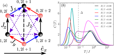
The KSM model describes bond-directional Ising interactions between spin $S=1/2$ operators Kitaev (2006). Its Hamiltonian in the presence of a magnetic field is given by (see also Fig. 1)

$$H_{S}=\sum_{\langle i,j\rangle}J^{a}_{ij}S_{i}^{a}S_{j}^{a}+g\mu_{B}\mathbf{B}\cdot\sum_{j}\mathbf{S}_{j}$$ (1)

with $J^{a}_{ij}$ the Kitaev interactions ($a=x,y,z$), $i,j$ nearest neighbor’s (NN) sites on the lattice, $g=1$ is the $g$-factor, $\mu_{B}=1$ the Bohr magneton, and $\mathbf{B}=(B,B,B)$ the magnetic field. We also set to unity the Planck and Boltzmann constants $\hbar,k_{B}=1$. The $J_{z}$-bonds in the middle of the hexagon arise from boundary conditions in the rung direction. Although the absence of these terms in Heisenberg Hamiltonians might give rise to new physics Luo et al. (2018), here they are not expected to play any role.

For $B=0$, KSM is characterized by a macroscopic number of local conservation laws, the so called flux (or vison) operators and due to that it becomes analytically solvable. The ground state sector resides in the uniform flux sector which is separated from other sectors by a gap $\Delta$. Here, we fix the Kitaev couplings to $J_{x}=2J$ and $J_{y}=J_{z}=J$, where the ground state is gapless, and we numerically determine $\Delta\simeq 0.07J$.

At finite temperatures the fluxes become thermally excited and a flux proliferation process occurs for $T<\Delta$. This behavior can be read off from the specific heat, $C(T)=\left(\langle H_{S}^{2}\rangle-\langle H_{S}\rangle^{2}\right)/T^{2}$, which is shown in Fig. 1 (b) for different values of the magnetic field $B$ Yoshitake et al. (2020); Patel and Trivedi (2019). The results are obtained from exact diagonalization for an $L=8$ rung system. For $B=0$, it exhibits the characteristic two-peak structure of Kitaev systems Nasu et al. (2014, 2015); Mishchenko et al. (2017); Metavitsiadis et al. (2017); Widmann et al. (2019). The low-temperature peak is associated with the flux proliferation, where the system gets flooded with flux excitations. The action with the Zeeman term creates an effective hopping term for the visons, making them effectively mobile Mandal et al. (2011). For $B<\Delta$, $C(T)$ remains practically unaffected indicating that the picture of the fluxes still holds. Intermediate magnetic fields reduce the height of the low-$T$ peak, which initially moves towards lower temperatures, characterizing a regime where visons are still present albeit mobile. For stronger $B$’s, the low temperature peak shifts to higher temperatures until it disappears, illustrating the absence of any trace of the fluxes.

Treating the magnetic field perturbatively for $B<\Delta$ enables a fermionic representation where spin operators are mapped into two species of Majorana fermions $c$ and $\bar{c}$ Kitaev (2006); You et al. (2012), with $\{c_{i},c_{j}\}=2\delta_{ij}=\{\bar{c}_{i},\bar{c}_{j}\}$ and $\{c_{i},\bar{c}_{j}\}=0$. One of the two species, say $c$, is itinerant, while the other pair up along the $z$-bond direction, they commute with the Hamiltonian, and they become static. We denote these local conservation laws with $\eta_{j}^{z}=\pm 1$ while we also introduce $\eta_{j}^{x}=\eta_{j}^{y}=1$ to unify the notation. The ground state occurs for $\eta_{j}^{z}=1$ while for $T\gg\Delta$ $\eta_{j}^{z}$ is completely disordered, $\langle\eta^{z}\rangle=0$. The magnetic field accounts for a TRS-breaking, NNN-interaction term in the fermionic representation, i.e., $H_{S}\approx H_{F}$ with

$$H_{F}=-\frac{i}{4}\sum_{\langle i,j\rangle}J^{a}_{ij}\eta_{i}^{a}c_{i}c_{j}-i\frac{J_{2}}{8}\sum_{\langle\langle i,j\rangle\rangle}\tilde{\eta}_{ij}c_{i}c_{j}~{},$$ (2)

and $J_{2}\sim\frac{B^{3}}{\Delta^{2}}$ Kitaev (2006); You et al. (2012); not (a). The double brackets in the second term denote summation over NNN sites and the order of the majorana pairs can be read off from Fig. 1(a). For $\tilde{\eta}$ holds: $\tilde{\eta}_{ij}=1$ for intrachain bonds or $\tilde{\eta}_{ij}=\eta_{i}^{z}+\eta_{j}^{z}$ for interchain bonds. In terms of Dirac fermions Feng et al. (2007); Chen and Nussinov (2008); Nussinov and Ortiz (2009); Mandal et al. (2012); Nussinov and van den Brink (2015), $H_{F}$ becomes a superconducting Hamiltonian on a two-site unit cell chain of length $L$, in the presence of an onsite $\mathbb{Z}_{2}$ gauge field $\sim\eta_{j}^{z}$ as well as bond disorder terms $\sim\tilde{\eta}_{ij}$.

Figure 2: System size scaling of the inverse participation ratio of the fermionic model, Eqs. (2) and (3), in a log-log scale for different values of the $J_{2}$ coupling. (a) Uniform gauge configuration. (b) Random average over $R=1000$ maximally disordered states, $\langle\eta^{z}\rangle=0$, and $3\sigma$ depicted as error bars.

¶Inverse participation ratio.

The first quantity that we look at in order to detect localization is the inverse participation ratio (IPR), which is given by the sum over the lattice sites of the squared probabilities of the wave-functions $\psi$ Evers and Mirlin (2008). For a given $\eta$-configuration, we denote the average IPR with $I_{\eta}$, while for disordered sectors, we average over $R$ gauge configurations to obtain the moments $\mathcal{I}_{p}$, viz.,

$$I_{\eta}=\frac{1}{L}\sum_{m=1}^{L}\sum_{l=1}^{L}|\psi_{m}^{\eta}(l)|^{4},\quad\mathcal{I}_{p}=\frac{1}{R}\sum_{r=1}^{R}\left(I_{\eta_{r}}\right)^{p}~{}.$$ (3)

From these definitions, the mean IPR is given by $\overline{I}=\mathcal{I}_{1}$ while the fluctuations around this mean can be quantified via the standard deviation $\sigma=\sqrt{\delta\overline{I}/R}$, where $\delta\overline{I}=\mathcal{I}_{2}-(\mathcal{I}_{1})^{2}$.

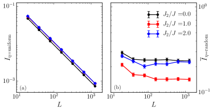
Assuming that all states of a system are localized $\psi_{m}^{\eta}(l)\sim\delta_{lm}$, the IPR is expected to scale as $\overline{I}(L)\sim\text{const.}$, while for extended states $\psi^{\eta}_{m}(l)\sim 1/\sqrt{L}$, $\overline{I}(L)\sim 1/L$. In Fig. 2(a), we plot in a log-log scale the IPR of the uniform gauge sector for different values of the $J_{2}$ coupling versus the system size, which reveals a $\sim 1/L$ scaling. On the contrary, for the same values of $J_{2}$, a random averaging over $R=1000$ sectors with $\langle\eta^{z}\rangle=0$ reveal the opposite behavior, namely $\overline{I}(L)\sim\text{const.}$. The difference between “clean” and “dirty” sectors is striking, and elucidates the localization character of the disordered states for any $J_{2}$. The initial drop of the IPR in Fig. 2(b) can be attributed to a comparable localization length $\xi$ with the system size. Moreover, from this behavior, it is hard to conclude a large sensitivity of $\xi$ to $J_{2}$.

¶Energy transport.

Figure 3: (a) Frequency dependence of the energy current correlation function in the fermionic representation, Eq. (2), for $J_{2}/J=0.026,1,2$ and $L=32$. For comparison, ${\mathcal{C}}(\omega)$ evaluated with $H_{S}$, for $B=0.05J$, and $L=8$ is also shown marked with cyan circles connected by a dotted line. (b) A zoom at low frequencies of (a). The lines depict second order polynomials, fitted in the range $0<\omega/J<0.07$ to extract the dc limit. (c) Finite size scaling of the Drude weight ${\mathcal{C}}_{0}$, in a semi-log plot. The lines are exponential fits.

Next we study the dynamical transport properties of $H_{F}$. For that, we employ the energy current dynamical auto-correlation function, which has the advantage to be diagonal in the gauge fields, and it is also directly related to the experimentally measurable thermal conductivity,

$${\mathcal{C}}(t)=\frac{1}{L}\left<j^{\epsilon}(t)j^{\epsilon}\right>,\quad{\mathcal{C}}(\omega)=\int dte^{i\omega t}{\mathcal{C}}(t)~{}.$$ (4)

Here, $j^{\epsilon}$ is the energy current operator, the exact expression of which is acquired via the time derivative of the polarization operator $j^{\epsilon}=\frac{\partial P}{\partial t}$ , $P=\sum_{l}r_{l}h_{l}$, with $h_{l}$ being a local energy density not (b) and $r_{l}$ its corresponding coordinate. The angled brackets denote a thermal expectation value, which here is restricted to infinite temperature. For the discussion of localization we are interested in the low-$\omega$ properties of ${\mathcal{C}}(\omega)$, and mainly its static part, which comprises two contributions: (i) the Drude weight arising from the non-vanishing due to degeneracies part of the correlation function at longer times, $2\pi{\mathcal{C}}_{0}=\lim_{t\rightarrow\infty}{\mathcal{C}}(t)$; (ii) the dc limit of the regular part ${\mathcal{C}}_{dc}=\lim_{\omega\rightarrow 0}{\mathcal{C}}(\omega)$. The former indicates ballistic while the latter dissipative transport and if both of them vanish, the system is an insulator.

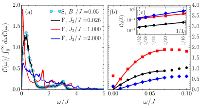
In Fig. 3(a), we present results for ${\mathcal{C}}(\omega)$, acquired via ED in the fermionic representation, for different values of the NNN interaction and $L=32$, corresponding to a Hilbert space dimension of $2^{64}$. Due to the different energy scales, we normalize the curves to a unit integral. In the fermionic representation, the quadratic form of $H_{F}$ yields two types of contributions in ${\mathcal{C}}$, “quasiparticle” or “pair-breaking”. These can be discerned in the curve for $J_{2}=0.026J$, corresponding to $B=0.05J<\Delta$. First, the maximum around $\omega\approx 0.4J$, is attributed to the quasiparticle part of the correlation function. The sharp decrease of ${\mathcal{C}}(\omega)$ at lower frequencies, $\omega\lesssim 0.2J$, better highlighted in Fig. 3(b), is inevitable due to the localization of the single particle states. Exactly the same behavior is recovered in the spin representation from the many-body Hamiltonian $H_{S}$, also plotted in Fig. 3(a), for $B/J=0.05$, and $L=8$. Second, the broader and of lower intensity hump, centered around $\omega\approx 3J$, corresponds to the pair-breaking type of contributions. As $J_{2}$ is further increased, the gap between the quasiparticle and the pair-breaking contributions is filled, however, as better seen in Fig. 3(b), the pseudo-gap at low frequencies does not close. In Fig. 3(b), we highlight the low frequency behavior of ${\mathcal{C}}(\omega)$ for the fermionic spectra plotted in panel (a). The lines connecting the points are second order polynomial fits in the range $0<\omega/J<0.07$, and extrapolate to tiny or even negative values at $\omega=0$ not (c). A small Drude weight ${\mathcal{C}}_{0}$ becomes also visible in Fig. 3(b), which finite size scaling behavior is plotted in Fig. 3(c) for systems $L=16-32$. The lines are exponential fits to the data and imply an exponential decay of $C_{0}$, namely, $C_{0}\rightarrow 0$ for $L\rightarrow\infty$. Thus, it can be inferred that both ${\mathcal{C}}_{0}$ and ${\mathcal{C}}_{dc}$ vanish in the thermodynamic limit.

As one of our prime results, we summarize the preceding by stating, that both the IPR and ${\mathcal{C}}(\omega)$ evidence, that a delocalization of the system cannot be captured within the fermionic representation despite the TRS-breaking nature of the NNN interaction induced by the magnetic field.

Figure 4: (a) Frequency dependence of the energy current correlation function in the spin representation, Eq. (1) for different values of the magnetic field, with $L=8$ (ED) and $L=12$ (DQT). (b) Finite size scaling of ${\mathcal{C}}(\omega)$ for $B=0.2J$.

¶Spin representation.

Next, we contrast the previous findings to ${\mathcal{C}}(\omega)$ obtained within the $H_{S}$ framework, where the magnetic field is taken fully into account, Eq. (1). To improve upon the available system sizes, facing the complete many body Hilbert space, and in addition to ED, we also employ Dynamical Quantum Typicality (DQT). In DQT a thermal mean value is approximated by an expectation value obtained from a single pure random state $|\psi\rangle$, drawn from a distribution that is invariant under all unitary transformations in Hilbert space (Haar measure), which leads to an exponential error decrease with $L$ Steinigeweg et al. (2014). The real part of correlation function is then evaluated via ${\mathcal{C}}^{\prime}(t)\approx\mathrm{Re}\frac{\langle\psi|j(t)j|\psi\rangle}{L\langle\psi|\psi\rangle}$ by solving a standard differential equation problem for the time evolution. The time evolution is performed with a $J\delta t=0.01$ step [corresponding to an accuracy of the order of $O(10^{-8})$ in the fourth order Runge-Kutta algorithm], while we integrate for times up to $Jt_{max}=100$.

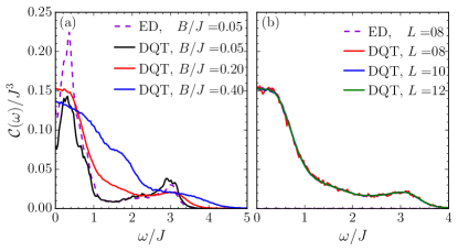
The results for ${\mathcal{C}}(\omega)$ for different values of $B$ are presented in Fig. 4(a). First, comparing DQT ($L=12$) and ED ($L=8$) at weak magnetic fields reveals a discrepancy between the two methods. This is due to the long time oscillations of the Kitaev terms, causing ${\mathcal{C}}(t)$ to oscillate even at the longest times kept here. These discrepancies disappear at higher magnetic fields where ${\mathcal{C}}(t_{max})=0$ and do not invalidate any of our conclusions, see also Fig. 4(b). As the magnetic field exceeds the gap, we observe a very rapid filling of the low frequency depletion. This can be interpreted as a large weakening of the fluxes’ scattering strength once they become mobile. Already at $B=0.2J$, the low frequency depletion disappears giving $C(\omega)$ a more Drude-like shape, although the higher frequency pair-breaking structure can still be observed. For even higher values of the magnetic field higher and lower frequencies are smoothly connected, while the dc limit shows only a weak dependence on $B>\Delta$. Thus one can argue, that $C_{dc}$, or equivalently the experimentally measurable thermal conductivity $\kappa_{dc}$, would exhibit a strong increase at $B\gtrsim\Delta$ followed by a weak variation as $B$ is further increased. Lastly in Fig. 4(b), we present the finite size scaling behavior of ${\mathcal{C}}(\omega)$, also comparing ED and DQT. We find, that there are practically no finite size effects at moderate magnetic fields in the data of the spin representation.

¶Discussion.

Our main finding here is, that fractionalization in the 1D-KSM, leading to a thermally activated flux disorder, induces self-localization for $B\lesssim\Delta$ and therefore leads to vanishing thermal transport coefficients. For stronger magnetic fields $B\gtrsim\Delta$, flux mobility and many-body interactions fill the low frequency depletion of ${\mathcal{C}}(\omega\ll 1)$ leading to delocalization and finite transport coefficients. The absence of this behavior in the popular simplification of the 1D-KSM, which treats magnetic fields only perturbatively, raises questions on the applicability of the latter model to describe finite-field transport.

Let us now speculate on the application of our results to the 2D-KSM. The characteristic low frequency depletion, attributed to the scattering of fermions on the gauge field Steinigeweg and Brenig (2016); Metavitsiadis and Brenig (2017), is also a characteristic of the 2D-KSM Nasu et al. (2017); Metavitsiadis et al. (2017); Pidatella et al. (2019). An essential difference in the absence of magnetic field between the 1D- and 2D-KSM is that in the latter, the pseudo-gap closes in the thermodynamic limit restoring dc transport. However, the mechanism of filling the low frequency depletion in the ${\mathcal{C}}(\omega)$ spectra due to the flux mobility will be also present in 2D. Taking into account that the flux gap of the 1D and the 2D systems are almost equal, $\Delta_{2D}\approx\Delta=0.07J$, and that typical values of Kitaev exchange are $J\approx 70K$, we expect $\Delta\approx 5K$. Therefore, a system with purely Kitaev interactions would exhibit a notable increase in the dc transport coefficients for magnetic fields around $B\gtrsim 7T$.

References

- Savary and Balents (2017) L. Savary and L. Balents, Reports on Progress in Physics 80, 016502 (2017), URL http://stacks.iop.org/0034-4885/80/i=1/a=016502.
- Zhou et al. (2017) Y. Zhou, K. Kanoda, and T.-K. Ng, Rev. Mod. Phys. 89, 025003 (2017), URL https://link.aps.org/doi/10.1103/RevModPhys.89.025003.
- Knolle and Moessner (2019) J. Knolle and R. Moessner, Annual Review of Condensed Matter Physics 10, 451 (2019), eprint https://doi.org/10.1146/annurev-conmatphys-031218-013401, URL https://doi.org/10.1146/annurev-conmatphys-031218-013401.
- Kitaev (2006) A. Kitaev, Annals of Physics 321, 2 (2006), ISSN 0003-4916, january Special Issue, URL http://www.sciencedirect.com/science/article/pii/S0003491605002381.
- Hermanns et al. (2018) M. Hermanns, I. Kimchi, and J. Knolle, Annual Review of Condensed Matter Physics 9, 17 (2018), eprint https://doi.org/10.1146/annurev-conmatphys-033117-053934, URL https://doi.org/10.1146/annurev-conmatphys-033117-053934.
- Stavropoulos et al. (2019) P. P. Stavropoulos, D. Pereira, and H.-Y. Kee, Phys. Rev. Lett. 123, 037203 (2019), URL https://link.aps.org/doi/10.1103/PhysRevLett.123.037203.
- Baskaran et al. (2008) G. Baskaran, D. Sen, and R. Shankar, Phys. Rev. B 78, 115116 (2008), URL https://link.aps.org/doi/10.1103/PhysRevB.78.115116.
- Rousochatzakis et al. (2018) I. Rousochatzakis, Y. Sizyuk, and N. B. Perkins, Nature Communications 9, 1575 (2018), ISSN 2041-1723, URL https://doi.org/10.1038/s41467-018-03934-1.
- Motome and Nasu (2020) Y. Motome and J. Nasu, Journal of the Physical Society of Japan 89, 012002 (2020), eprint https://doi.org/10.7566/JPSJ.89.012002, URL https://doi.org/10.7566/JPSJ.89.012002.
- Feng et al. (2007) X.-Y. Feng, G.-M. Zhang, and T. Xiang, Phys. Rev. Lett. 98, 087204 (2007), URL https://link.aps.org/doi/10.1103/PhysRevLett.98.087204.
- Wu (2012) N. Wu, Physics Letters A 376, 3530 (2012), ISSN 0375-9601, URL http://www.sciencedirect.com/science/article/pii/S0375960112010444.
- Steinigeweg and Brenig (2016) R. Steinigeweg and W. Brenig, Phys. Rev. B 93, 214425 (2016), URL https://link.aps.org/doi/10.1103/PhysRevB.93.214425.
- Metavitsiadis and Brenig (2017) A. Metavitsiadis and W. Brenig, Phys. Rev. B 96, 041115 (2017), URL https://link.aps.org/doi/10.1103/PhysRevB.96.041115.
- Metavitsiadis et al. (2019) A. Metavitsiadis, C. Psaroudaki, and W. Brenig, Phys. Rev. B 99, 205129 (2019), URL https://link.aps.org/doi/10.1103/PhysRevB.99.205129.
- Agrapidis et al. (2019) C. E. Agrapidis, J. van den Brink, and S. Nishimoto, Phys. Rev. B 99, 224418 (2019), URL https://link.aps.org/doi/10.1103/PhysRevB.99.224418.
- Anderson (1958) P. W. Anderson, Phys. Rev. 109, 1492 (1958), URL https://link.aps.org/doi/10.1103/PhysRev.109.1492.
- Nandkishore and Huse (2015) R. Nandkishore and D. A. Huse, Annual Review of Condensed Matter Physics 6, 15 (2015), eprint https://doi.org/10.1146/annurev-conmatphys-031214-014726, URL https://doi.org/10.1146/annurev-conmatphys-031214-014726.
- Alet and Laflorencie (2018) F. Alet and N. Laflorencie, Comptes Rendus Physique 19, 498 (2018), ISSN 1631-0705, quantum simulation / Simulation quantique, URL http://www.sciencedirect.com/science/article/pii/S163107051830032X.
- Kagan and Maksimov (1984) Y. Kagan and L. A. Maksimov, JETP 60, 201 (1984), [Russian original - ZhETF, 87, 348 (1984)], URL http://www.jetp.ac.ru/cgi-bin/e/index/e/60/1/p201?a=list.
- Nandkishore and Hermele (2019) R. M. Nandkishore and M. Hermele, Annual Review of Condensed Matter Physics 10, 295 (2019), eprint https://doi.org/10.1146/annurev-conmatphys-031218-013604, URL https://doi.org/10.1146/annurev-conmatphys-031218-013604.
- De Roeck and Huveneers (2014) W. De Roeck and F. m. c. Huveneers, Phys. Rev. B 90, 165137 (2014), URL https://link.aps.org/doi/10.1103/PhysRevB.90.165137.
- Schiulaz et al. (2015) M. Schiulaz, A. Silva, and M. Müller, Phys. Rev. B 91, 184202 (2015), URL https://link.aps.org/doi/10.1103/PhysRevB.91.184202.
- Yao et al. (2016) N. Y. Yao, C. R. Laumann, J. I. Cirac, M. D. Lukin, and J. E. Moore, Phys. Rev. Lett. 117, 240601 (2016), URL https://link.aps.org/doi/10.1103/PhysRevLett.117.240601.
- Smith et al. (2017) A. Smith, J. Knolle, D. L. Kovrizhin, and R. Moessner, Phys. Rev. Lett. 118, 266601 (2017), URL https://link.aps.org/doi/10.1103/PhysRevLett.118.266601.
- Mondaini and Cai (2017) R. Mondaini and Z. Cai, Phys. Rev. B 96, 035153 (2017), URL https://link.aps.org/doi/10.1103/PhysRevB.96.035153.
- Michailidis et al. (2018) A. A. Michailidis, M. Žnidarič, M. Medvedyeva, D. A. Abanin, T. c. v. Prosen, and Z. Papić, Phys. Rev. B 97, 104307 (2018), URL https://link.aps.org/doi/10.1103/PhysRevB.97.104307.
- Mamaev et al. (2019) M. Mamaev, I. Kimchi, M. A. Perlin, R. M. Nandkishore, and A. M. Rey, Phys. Rev. Lett. 123, 130402 (2019), URL https://link.aps.org/doi/10.1103/PhysRevLett.123.130402.
- Brenes et al. (2018) M. Brenes, M. Dalmonte, M. Heyl, and A. Scardicchio, Phys. Rev. Lett. 120, 030601 (2018), URL https://link.aps.org/doi/10.1103/PhysRevLett.120.030601.
- Yarloo et al. (2019) H. Yarloo, M. Mohseni-Rajaee, and A. Langari, Phys. Rev. B 99, 054403 (2019), URL https://link.aps.org/doi/10.1103/PhysRevB.99.054403.
- Sala et al. (2020) P. Sala, T. Rakovszky, R. Verresen, M. Knap, and F. Pollmann, Phys. Rev. X 10, 011047 (2020), URL https://link.aps.org/doi/10.1103/PhysRevX.10.011047.
- Jackeli and Khaliullin (2009) G. Jackeli and G. Khaliullin, Phys. Rev. Lett. 102, 017205 (2009), URL https://link.aps.org/doi/10.1103/PhysRevLett.102.017205.
- Chaloupka et al. (2010) J. c. v. Chaloupka, G. Jackeli, and G. Khaliullin, Phys. Rev. Lett. 105, 027204 (2010), URL http://link.aps.org/doi/10.1103/PhysRevLett.105.027204.
- Takagi et al. (2019) H. Takagi, T. Takayama, G. Jackeli, G. Khaliullin, and S. E. Nagler, Kitaev quantum spin liquid - concept and materialization (2019), eprint 1903.08081.
- Plumb et al. (2014) K. W. Plumb, J. P. Clancy, L. J. Sandilands, V. V. Shankar, Y. F. Hu, K. S. Burch, H.-Y. Kee, and Y.-J. Kim, Phys. Rev. B 90, 041112 (2014), URL https://link.aps.org/doi/10.1103/PhysRevB.90.041112.
- Nussinov and van den Brink (2015) Z. Nussinov and J. van den Brink, Rev. Mod. Phys. 87, 1 (2015), URL https://link.aps.org/doi/10.1103/RevModPhys.87.1.
- Banerjee et al. (2016) A. Banerjee, C. A. Bridges, J.-Q. Yan, A. A. Aczel, L. Li, M. B. Stone, G. E. Granroth, M. D. Lumsden, Y. Yiu, J. Knolle, et al., Nat. Mater. advance online publication (2016), URL http://dx.doi.org/10.1038/nmat4604.
- Choi et al. (2012) S. K. Choi, R. Coldea, A. N. Kolmogorov, T. Lancaster, I. I. Mazin, S. J. Blundell, P. G. Radaelli, Y. Singh, P. Gegenwart, K. R. Choi, et al., Phys. Rev. Lett. 108, 127204 (2012), URL https://link.aps.org/doi/10.1103/PhysRevLett.108.127204.
- Nishimoto et al. (2016) S. Nishimoto, V. M. Katukuri, V. Yushankhai, H. Stoll, U. K. Rößler, L. Hozoi, I. Rousochatzakis, and J. van den Brink, Nature Communications 7, 10273 (2016), ISSN 2041-1723, URL https://doi.org/10.1038/ncomms10273.
- Yadav et al. (2016) R. Yadav, N. A. Bogdanov, V. M. Katukuri, S. Nishimoto, J. van den Brink, and L. Hozoi, Scientific Reports 6, 37925 (2016), ISSN 2045-2322, URL https://doi.org/10.1038/srep37925.
- Kitagawa et al. (2018) K. Kitagawa, T. Takayama, Y. Matsumoto, A. Kato, R. Takano, Y. Kishimoto, S. Bette, R. Dinnebier, G. Jackeli, and H. Takagi, Nature 554, 341 (2018), ISSN 1476-4687, URL https://doi.org/10.1038/nature25482.
- Wulferding et al. (2020) D. Wulferding, Y. Choi, S.-H. Do, C. H. Lee, P. Lemmens, C. Faugeras, Y. Gallais, and K.-Y. Choi, Nature Communications 11, 1603 (2020), ISSN 2041-1723, URL https://doi.org/10.1038/s41467-020-15370-1.
- Duan et al. (2003) L.-M. Duan, E. Demler, and M. D. Lukin, Phys. Rev. Lett. 91, 090402 (2003), URL https://link.aps.org/doi/10.1103/PhysRevLett.91.090402.
- Schreiber et al. (2015) M. Schreiber, S. S. Hodgman, P. Bordia, H. P. Lüschen, M. H. Fischer, R. Vosk, E. Altman, U. Schneider, and I. Bloch, Science 349, 842 (2015), ISSN 0036-8075, eprint https://science.sciencemag.org/content/349/6250/842.full.pdf, URL https://science.sciencemag.org/content/349/6250/842.
- Barbiero et al. (2019) L. Barbiero, C. Schweizer, M. Aidelsburger, E. Demler, N. Goldman, and F. Grusdt, Science Advances 5 (2019), eprint https://advances.sciencemag.org/content/5/10/eaav7444.full.pdf, URL https://advances.sciencemag.org/content/5/10/eaav7444.
- Economou (2006) E. Economou, Green’s Functions in Quantum Physics, Springer Series in Solid-State Sciences (Springer, 2006), ISBN 9783540122661, URL https://link.springer.com/book/10.1007/3-540-28841-4.
- Kasahara et al. (2018a) Y. Kasahara, T. Ohnishi, Y. Mizukami, O. Tanaka, S. Ma, K. Sugii, N. Kurita, H. Tanaka, J. Nasu, Y. Motome, et al., Nature 559, 227 (2018a), ISSN 1476-4687, URL https://doi.org/10.1038/s41586-018-0274-0.
- Kasahara et al. (2018b) Y. Kasahara, K. Sugii, T. Ohnishi, M. Shimozawa, M. Yamashita, N. Kurita, H. Tanaka, J. Nasu, Y. Motome, T. Shibauchi, et al., Phys. Rev. Lett. 120, 217205 (2018b), URL https://link.aps.org/doi/10.1103/PhysRevLett.120.217205.
- Hentrich et al. (2019) R. Hentrich, M. Roslova, A. Isaeva, T. Doert, W. Brenig, B. Büchner, and C. Hess, Phys. Rev. B 99, 085136 (2019), URL https://link.aps.org/doi/10.1103/PhysRevB.99.085136.
- Yokoi et al. (2020) T. Yokoi, S. Ma, Y. Kasahara, S. Kasahara, T. Shibauchi, N. Kurita, H. Tanaka, J. Nasu, Y. Motome, C. Hickey, et al., Half-integer quantized anomalous thermal hall effect in the kitaev material -rucl3 (2020), eprint 2001.01899.
- Vinkler-Aviv and Rosch (2018) Y. Vinkler-Aviv and A. Rosch, Phys. Rev. X 8, 031032 (2018), URL https://link.aps.org/doi/10.1103/PhysRevX.8.031032.
- Ye et al. (2018) M. Ye, G. B. Halász, L. Savary, and L. Balents, Phys. Rev. Lett. 121, 147201 (2018), URL https://link.aps.org/doi/10.1103/PhysRevLett.121.147201.
- Yu et al. (2018) Y. J. Yu, Y. Xu, K. J. Ran, J. M. Ni, Y. Y. Huang, J. H. Wang, J. S. Wen, and S. Y. Li, Phys. Rev. Lett. 120, 067202 (2018), URL https://link.aps.org/doi/10.1103/PhysRevLett.120.067202.
- Hentrich et al. (2018) R. Hentrich, A. U. B. Wolter, X. Zotos, W. Brenig, D. Nowak, A. Isaeva, T. Doert, A. Banerjee, P. Lampen-Kelley, D. G. Mandrus, et al., Phys. Rev. Lett. 120, 117204 (2018), URL https://link.aps.org/doi/10.1103/PhysRevLett.120.117204.
- Hirobe et al. (2017) D. Hirobe, M. Sato, Y. Shiomi, H. Tanaka, and E. Saitoh, Phys. Rev. B 95, 241112 (2017), URL https://link.aps.org/doi/10.1103/PhysRevB.95.241112.
- Leahy et al. (2017) I. A. Leahy, C. A. Pocs, P. E. Siegfried, D. Graf, S.-H. Do, K.-Y. Choi, B. Normand, and M. Lee, Phys. Rev. Lett. 118, 187203 (2017), URL https://link.aps.org/doi/10.1103/PhysRevLett.118.187203.
- Nasu et al. (2017) J. Nasu, J. Yoshitake, and Y. Motome, Phys. Rev. Lett. 119, 127204 (2017), URL https://link.aps.org/doi/10.1103/PhysRevLett.119.127204.
- Metavitsiadis et al. (2017) A. Metavitsiadis, A. Pidatella, and W. Brenig, Phys. Rev. B 96, 205121 (2017), URL https://link.aps.org/doi/10.1103/PhysRevB.96.205121.
- Pidatella et al. (2019) A. Pidatella, A. Metavitsiadis, and W. Brenig, Phys. Rev. B 99, 075141 (2019), URL https://link.aps.org/doi/10.1103/PhysRevB.99.075141.
- Luo et al. (2018) Q. Luo, S. Hu, J. Zhao, A. Metavitsiadis, S. Eggert, and X. Wang, Phys. Rev. B 97, 214433 (2018), URL https://link.aps.org/doi/10.1103/PhysRevB.97.214433.
- Yoshitake et al. (2020) J. Yoshitake, J. Nasu, Y. Kato, and Y. Motome, Phys. Rev. B 101, 100408 (2020), URL https://link.aps.org/doi/10.1103/PhysRevB.101.100408.
- Patel and Trivedi (2019) N. D. Patel and N. Trivedi, Proceedings of the National Academy of Sciences 116, 12199 (2019), ISSN 0027-8424, eprint https://www.pnas.org/content/116/25/12199.full.pdf, URL https://www.pnas.org/content/116/25/12199.
- Nasu et al. (2014) J. Nasu, M. Udagawa, and Y. Motome, Phys. Rev. Lett. 113, 197205 (2014), URL https://link.aps.org/doi/10.1103/PhysRevLett.113.197205.
- Nasu et al. (2015) J. Nasu, M. Udagawa, and Y. Motome, Phys. Rev. B 92, 115122 (2015), URL https://link.aps.org/doi/10.1103/PhysRevB.92.115122.
- Mishchenko et al. (2017) P. A. Mishchenko, Y. Kato, and Y. Motome, Phys. Rev. B 96, 125124 (2017), URL https://link.aps.org/doi/10.1103/PhysRevB.96.125124.
- Widmann et al. (2019) S. Widmann, V. Tsurkan, D. A. Prishchenko, V. G. Mazurenko, A. A. Tsirlin, and A. Loidl, Phys. Rev. B 99, 094415 (2019), URL https://link.aps.org/doi/10.1103/PhysRevB.99.094415.
- Mandal et al. (2011) S. Mandal, S. Bhattacharjee, K. Sengupta, R. Shankar, and G. Baskaran, Phys. Rev. B 84, 155121 (2011), URL https://link.aps.org/doi/10.1103/PhysRevB.84.155121.
- You et al. (2012) Y.-Z. You, I. Kimchi, and A. Vishwanath, Phys. Rev. B 86, 085145 (2012), URL https://link.aps.org/doi/10.1103/PhysRevB.86.085145.
- not (a) Although for to be valid, here we treat it as a free parameter to be able to detect a possible delocalization due to the TRS term.
- Chen and Nussinov (2008) H.-D. Chen and Z. Nussinov, Journal of Physics A: Mathematical and Theoretical 41, 075001 (2008), URL https://doi.org/10.1088%2F1751-8113%2F41%2F7%2F075001.
- Nussinov and Ortiz (2009) Z. Nussinov and G. Ortiz, Phys. Rev. B 79, 214440 (2009), URL https://link.aps.org/doi/10.1103/PhysRevB.79.214440.
- Mandal et al. (2012) S. Mandal, R. Shankar, and G. Baskaran, Journal of Physics A: Mathematical and Theoretical 45, 335304 (2012), URL https://doi.org/10.1088%2F1751-8113%2F45%2F33%2F335304.
- Evers and Mirlin (2008) F. Evers and A. D. Mirlin, Rev. Mod. Phys. 80, 1355 (2008), URL https://link.aps.org/doi/10.1103/RevModPhys.80.1355.
- not (b) The unit cell chosen here is a linear combination of the one shown in Fig. 1 with the last -bond removed and the same one only shifted by one-rung, see also Refs. Metavitsiadis and Brenig (2017); Metavitsiadis et al. (2019). We have also tested other choices, which give no qualitative difference but at most some quantitative discrepancies at high frequencies.
- not (c) Even the tiny finite values can be shown that go to zero as by using an averaging over gauge configurations which allows to reach much larger system sizes Metavitsiadis and Brenig (2017).
- Steinigeweg et al. (2014) R. Steinigeweg, J. Gemmer, and W. Brenig, Phys. Rev. Lett. 112, 120601 (2014), URL http://link.aps.org/doi/10.1103/PhysRevLett.112.120601.