Sharp isoperimetric inequalities for infinite plane graphs with bounded vertex and face degrees

Abstract.

We give sharp bounds for isoperimetric constants of infinite plane graphs(tessellations) with bounded vertex and face degrees. For example if $G$ is a plane graph satisfying the inequalities $p_{1}\leq\deg v\leq p_{2}$ for $v\in V(G)$ and $q_{1}\leq\deg f\leq q_{2}$ for $f\in F(G)$, where $p_{1},p_{2},q_{1}$, and $q_{2}$ are natural numbers such that $1/p_{i}+1/q_{i}\leq 1/2$, $i=1,2$, then we show that

$$\Phi(p_{1},q_{1})\leq\inf_{S}\frac{|\partial S|}{|V(S)|}\leq\Phi(p_{2},q_{2}),$$

where the infimum is taken over all finite nonempty subgraphs $S\subset G$, $\partial S$ is the set of edges connecting $S$ to $G\setminus S$, and $\Phi(p,q)$ is defined by

$$\Phi(p,q)=(p-2)\sqrt{1-\frac{4}{(p-2)(q-2)}}.$$

For $p_{1}=3$ this gives an affirmative answer for a conjecture by Lawrencenko, Plummer, and Zha from 2002, and for general $p_{i}$ and $q_{i}$ our result fully resolves a question in the book by Lyons and Peres from 2016, where they extended the conjecture of Lawrencenko et al. to the above form. We also prove a discrete analogue of Weil’s isoperimetric theorem, extending a result of Angel, Benjamini, and Horesh from 2018, and give a positive answer for a problem asked by Angel et al. in the same paper.

1. Introduction

Graphs considered in this paper are infinite tessellations of the plane, on which we study geometric and topological properties of the graph and prove sharp isoperimetric inequalities. In particular we give an affirmative answer for Question 6.21 in the book by Lyons and Peres [49] as well as Conjecture 1.1 by Lawrencenko, Plummer, and Zha [47]. We also prove a discrete analogue of Weil’s isoperimetric theorem for non-positively curved surface, extending a result of Angel, Benjamini, and Horesh [3, Theorem 1.2], and give a positive answer for [3, Problem 3.2] by Angel et al. The main tool is the combinatorial Gauss-Bonnet theorem involving left turns(geodesic curvature), and we have obtained the results by interpreting left turns of the boundary curves combinatorially. The background and motivation of our research is the following.

Suppose $\mathcal{M}$ is a complete simply connected open 2-dimensional Riemannian manifold whose Gaussian curvature is bounded above by $k<0$. Then one can prove using the famous Cartan-Hadamard theorem that

(1.1) $$\inf_{\Omega}\left\{\frac{\mbox{length}(b\Omega)}{\mbox{area}(\Omega)}\right\}\geq\sqrt{-k},$$

where the infimum is taken over all finite regions $\Omega\subset\mathcal{M}$ with smooth boundaries $b\Omega$ (cf. [13, Theorem 34.2.6]). The constant(infimum) on the left hand side of (1.1) is called the isoperimetric constant of $\mathcal{M}$, or the Cheeger constant named after Jeff Cheeger [14], and known to be equal to $\sqrt{-k}$ for the hyperbolic plane of constant curvature $k<0$.

It might be natural to expect a similar phenomenon for discrete cases. Let us choose a plane graph $G$ as a discrete analogue of a 2-dimensional Riemannian manifold, and note that curvature on a plane graph is usually described in terms of vertex and face degrees. (See Section 2 for notation and terminology, and Section 3 for the concept and properties of combinatorial curvatures.) Thus a counterpart of a simply connected 2-dimensional Riemannian manifold of constant Gaussian curvature is a $(p,q)$-regular graph $G$, a tessellation of the plane with $\deg v=p$ for all $v\in V=V(G)$ and $\deg f=q$ for all $f\in F=F(G)$, where $p$ and $q$ are natural numbers greater than or equal to $3$, $V$ and $F$ are the vertex and face sets of $G$, respectively, and $\deg a$ denotes the degree of $a\in V\cup F$ (the number of edges incident to $a$). In this setting Riemannian manifolds whose curvatures are bounded from above would correspond to tessellations of the plane with vertex and face degrees bounded from below, say by $p$ and $q$, respectively.

There are several options for a discrete analogue to the isoperimetric constant. Let $S$ be a subgraph of a given tessellation $G$, and we define the edge boundary $\partial S$ of $S$ as the set of edges in $E=E(G)$ with one end on $V(S)$ and the other end on $V\setminus V(S)$, where $E$ is the edge set of $G$. Also we define the boundary walk $bS$ of $S$ as the sequence of edges traversed by those who walk along the topological boundary of $S$ in the positive direction. See Section 2 for the precise definition of $bS$, but at this point one may think of it as the set of edges in $E(S)$ that are included in the boundaries of faces in $F\setminus F(S)$. Now the isoperimetric constants, which are also known as the Cheeger constants as in the continuous case, of $G$ are defined by the formulae

(1.2) $$\imath(G)=\inf_{S}\frac{|\partial S|}{|V(S)|},\qquad \imath^{*}(G)=\inf_{S}\frac{|bS|}{|F(S)|},$$

$$\imath_{\sigma}(G)=\inf_{S}\frac{|\partial S|}{\sum_{v\in V(S)}\deg v},\qquad \imath_{\sigma}^{*}(G)=\inf_{S}\frac{|bS|}{\sum_{f\in F(S)}\deg f},$$

where the infima are taken over all finite nonempty subgraphs $S\subset G$ and $|\cdot|$ is the cardinality of the given set. Here it is also assumed that $F(S)\neq\emptyset$ for $\imath^{*}(G)$ and $\imath_{\sigma}^{*}(G)$.

Isoperimetric constants have been studied extensively in graph theory, because they are related to many important properties of the structures and therefore have many applications. See for instance [4, 51] and the references therein. The constants $\imath(G)$ and $\imath_{\sigma}(G)$ are the most common isoperimetric constants, because they can be defined for every type of graphs including non-planar graphs, disconnected graphs, and finite graphs (with some modification in the definition), and more importantly, because they have many applications to spectral theory on graphs, simple random walks, etc. For example, $\imath(G)$ and $\imath_{\sigma}(G)$ are used to bound the bottom of the spectrum of negative combinatorial Laplacian [21, 22, 23, 25, 41, 42, 44, 46, 50, 52]. These constants also appear on various settings [3, 4, 8, 9, 32, 33, 34, 35, 40, 43, 48, 49, 51, 53, 54, 56, 57, 61, 63, 70, 71, and more]. For $\imath^{*}(G)$ and $\imath^{*}_{\sigma}(G)$, they are defined by imitating the isoperimetric constants on Riemannian manifolds, hence these constants logically make sense only for graphs embedded into 2-dimensional manifolds. The constants $\imath^{*}(G)$ or $\imath^{*}_{\sigma}(G)$ are found in [34, 35, 47, 53, 58, 61], and positivity of these constants implies Gromov hyperbolicity of the graph, provided that face degrees are bounded [57, 58]. Note that $\imath^{*}(G)$ and $\imath^{*}_{\sigma}(G)$ are the duals of $\imath(G)$ and $\imath_{\sigma}(G)$, respectively; i.e., we have $\imath(G)=\imath^{*}(G^{*})$ and $\imath_{\sigma}(G)=\imath_{\sigma}^{*}(G^{*})$, where $G^{*}$ is the dual graph of $G$.

Now let us go back to the problem considered at the beginning, and suppose that $G$ is a $(p,q)$-regular graph with $p,q\geq 3$. If $1/p+1/q>1/2$, then $G$ is in fact a finite graph and a tessellation of the Riemann sphere, which is not what we are studying in this paper. Anyway in this case $G$ becomes one of the platonic solids; i.e., G is one of the tetrahedron, the octahedron, the icosahedron, the cube, or the dodecahedron (Figure 1).

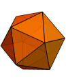
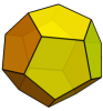
Figure 1. Platonic solids

The case $1/p+1/q=1/2$ happens if and only if $(p,q)\in\{(6,3),(4,4),(3,6)\}$, hence in this case $G$ is infinite and becomes one of the regular tilings of the plane; i.e., $G$ is the $6$-regular triangulation of the plane if $(p,q)=(6,3)$, the square lattice if $(p,q)=(4,4)$, and the hexagonal honeycomb if $(p,q)=(3,6)$ (Figure 2). Graphs in this category correspond to simply connected 2-dimensional Riemannian manifolds of constant zero curvature (i.e., the Euclidean plane), and have zero isoperimetric constants in (1.2).

Figure 2. Regular tilings of the plane

The case we are mostly interested in is when $1/p+1/q<1/2$; in this case the $(p,q)$-regular graph corresponds to a hyperbolic plane of constant negative curvature, and the isoperimetric constants in (1.2) are positive [34, 70, 71]. Moreover, the precise isoperimetric constants of $(p,q)$-regular graphs are computed independently by two groups of researchers, Häggström, Jonasson, and Lyons [32] and Higuchi and Shirai [35], and their results can be summarized as follows.

Theorem 1.

Suppose $G$ is a $(p,q)$-regular graph for some integers $p,q\geq 3$ satisfying $1/p+1/q\leq 1/2$. Then we have

$$\imath(G) =\Phi(p,q)\quad \imath^{*}(G) =\Phi(q,p),$$

$$\imath_{\sigma}(G) =\Phi(p,q)/p,\quad \imath_{\sigma}^{*}(G) =\Phi(q,p)/q,$$

where

$$\Phi(a,b)=(a-2)\sqrt{1-\frac{4}{(a-2)(b-2)}}.$$

As we discussed above, a discrete counterpart of a Riemannian manifold whose curvature is bounded above by a negative number is a tessellation $G$ of the plane such that $\deg v\geq p$ for all $v\in V$ and $\deg f\geq q$ for all $f\in F$, where $p,q$ are natural numbers satisfying $1/p+1/q<1/2$. Then as in the continuous case (1.1), one can expect that the isoperimetric constants of $G$ are bounded below by those of the $(p,q)$-regular graph; i.e., we can predict for example that

(1.3) $$\imath^{*}(G)\geq\Phi(q,p)=(q-2)\sqrt{1-\frac{4}{(p-2)(q-2)}},$$

and similar expectation would apply to the other isoperimetric constants. For this reason the inequality (1.3) was conjectured by Lawrencenko et al. [47, Conjecture 1.1] for the case $q=3$ (for $q>3$ it was also conjectured in the same paper [47], but only implicitly).

Conversely if $G$ is an infinite tessellation of the plane and if $\deg v\leq p$ and $\deg f\leq q$ for all $v\in V$ and $f\in F$, where $p$ and $q$ are as before, then it is also natural to expect that the isoperimetric constants of $G$ are not greater than those of the $(p,q)$-regular graphs. In this context Lyons and Peres posed the following question in [49, Question 6.21].

Question 2.

Suppose $G=(V,E,F)$ is a plane graph satisfying the inequalities $p_{1}\leq\deg v\leq p_{2}$ for all $v\in V(G)$ and $q_{1}\leq\deg f\leq q_{2}$ for all $f\in F(G)$, where $p_{1},p_{2},q_{1}$, and $q_{2}$ are natural numbers such that $1/p_{i}+1/q_{i}\leq 1/2$, $i=1,2$. Then does it always hold

$$\Phi(p_{1},q_{1})\leq\imath(G)\leq\Phi(p_{2},q_{2})\,?$$

Before stating our results, let us briefly describe some known estimates for isoperimetric constants. The first known such estimate is due to Dodziuk [22], who proved that if $G$ is a triangulation (i.e., $\deg f=3$ for every face $f$) and $\deg v\geq 7$ for every $v\in V=V(G)$, then we have

$$\imath^{*}(G)\geq\frac{1}{26}.$$

Dodziuk and Kendall also proved in [21] that

$$\imath_{\sigma}(G)\geq\frac{1}{78}$$

for triangulations $G$ with $\deg v\geq 7$ for every $v\in V$. On the other hand, Dodziuk’s bound for $\imath^{*}(G)$ was significantly improved by Mohar [53] such as

$$\imath^{*}(G)\geq\frac{p-6}{p-4},$$

where $G$ is a triangulation of the plane with $\deg v\geq p\geq 7$ for all $v\in V$, and this result was further improved by Lawrencenko et al.  [47] such as

$$\imath^{*}(G)\geq\frac{(p-6)(p^{2}-8p+15)}{(p-4)(p^{2}-8p+13)}.$$

When $G$ is a tessellation of the plane with $\deg v\geq p$ for all $v\in V$ and $\deg f\geq q$ for all $f\in F$, where $p,q$ are natural numbers such that $1/p+1/q<1/2$, it was shown by Mohar [54] that

$$\imath(G)\geq\frac{pq-2p-2q}{3q-8}.$$

Also see [44], where the constants $\imath(G)$ and $\imath_{\sigma}(G)$ are estimated in terms of (vertex) combinatorial curvature. (See Section 3 for the definition of combinatorial curvature.)

Now we present that

Theorem 3.

Suppose $G=(V,E,F)$ is a plane graph such that $p\leq\deg v<\infty$ and $q\leq\deg f<\infty$ for all $v\in V$ and $f\in F$, where $p$ and $q$ are natural numbers satisfying $1/p+1/q\leq 1/2$. Then we have

$$\imath(G) \geq\Phi(p,q)\quad \imath^{*}(G) \geq\Phi(q,p),$$

$$\imath_{\sigma}(G) \geq\Phi(p,q)/p,\quad \imath_{\sigma}^{*}(G) \geq\Phi(q,p)/q.$$

The conclusions of Theorem 3 remain true even when $G$ has some infinigons; i.e., $G$ has some faces $f$ with $\deg f=\infty$. See Section 9 for details. We have excluded infinigons from the statement of Theorem 3 just for simplicity, because our bounds for $\imath(G)$ and $\imath_{\sigma}(G)$ are obtained through dual graphs. Meanwhile, it is worth to mention that the graph $G$ in Theorem 3 must be an infinite tessellation of the plane, because its corner curvature is always negative. See [41, Theorem 1].

We next provide our second result, which is about upper bounds for isoperimetric constants.

Theorem 4.

Suppose $G=(V,E,F)$ is an infinite tessellation of the plane such that $\deg v\leq p$ and $\deg f\leq q$ for all $v\in V$ and $f\in F$, where $p$ and $q$ are natural numbers satisfying $1/p+1/q\leq 1/2$. Then we have

$$\imath(G) \leq\Phi(p,q)\quad \imath^{*}(G) \leq\Phi(q,p),$$

$$\imath_{\sigma}(G) \leq\Phi(p,q)/p,\quad \imath_{\sigma}^{*}(G) \leq\Phi(q,p)/q.$$

Note that Theorems 3 and 4 together completely resolve Question 2 as well as the conjecture by Lawrencenko et al., and our results are the best possible because the isoperimetric constants of $(p,q)$-regular graphs are the lower and upper bounds in Theorems 3 and 4, respectively.

Our next result can be characterized as a discrete version of Weil’s isoperimetric theorem. In 1926 Weil proved [69] (cf. [38]) that if $\mathcal{M}$ is a 2-dimensional Riemannian manifold whose Gaussian curvature is non-positive everywhere, the inequality

$$|b\Omega|\geq 2\sqrt{\pi\cdot\mbox{Area}(\Omega)}$$

holds for every domain $\Omega\subset\mathcal{M}$ homeomorphic to the unit disk. Then one may expect a similar phenomenon in the discrete setting as well, and in this context Angel, Benjamini, and Horesh proved the following theorem [3, Theorem 1.2].

Theorem 5.

Let $G=(V,E,F)$ be a plane graph such that $\deg v\geq 6$ and $\deg f\geq 3$ for every $v\in V$ and $f\in F$, respectively. If $S\subset G$ is a finite subgraph such that $|V(bS)|=n$, then we have

$$|V(S)|\leq\left\lfloor\frac{n^{2}}{12}+\frac{n}{2}+1\right\rfloor.$$

The equality can be achieved in certain subgraphs of the $6$-regular triangulation of the plane.

We have considered that $(p,q)$-regular graphs with $(p,q)\in\{(6,3),(4,4),(3,6)\}$ are the discrete counterparts of the Euclidean plane, and Theorem 5 deals with the case $(p,q)=(6,3)$. Thus we wished to extend Theorem 5 to the other counterparts of the Euclidean plane as well, and have obtained the following result.

Theorem 6.

Let $G=(V,E,F)$ be a plane graph such that $\deg v\geq p$ and $\deg f\geq q$ for every $v\in V$ and $f\in F$, respectively, where $p,q$ are natural numbers such that $1/p+1/q=1/2$. If $S\subset G$ is a finite subgraph satisfying $|V(bS)|=n$, then we have

(1.4) $$|V(S)|\leq\left\lfloor\frac{n^{2}}{4q}+\frac{n}{2}+1\right\rfloor$$

if $q=3$ or $4$, and

(1.5) $$|V(S)|\leq\left\lfloor\frac{n^{2}}{4q}+\frac{n}{2}+\frac{3}{2}\right\rfloor=\left\lfloor\frac{n^{2}}{24}+\frac{n}{2}+\frac{3}{2}\right\rfloor$$

if $q=6$.

One can ask when equality holds in (1.4) or (1.5). Theorem 5 says that it can be achieved in certain subgraphs of the $6$-regular triangulation of the plane, and we could make it explicit as follows.

Theorem 7.

Let $G$ be a regular tiling of the plane; i.e., $G$ is a $(p,q)$-regular graph for some $(p,q)\in\{(6,3),(4,4),(3,6)\}$. Then there exists $S\subset G$ for which equality holds in (1.4) or (1.5) (with $|V(bS)|=n$) if and only if one of the following holds:

1. $q=3$ and $n\in\mathbb{N}$;

2. $q=4$, and $n$ is $1$ or a positive even integer;

3. $q=6$, and $n$ is $1$ or a positive even integer such that $n\not\equiv 4,8\pmod{12}$.

If $G$ is either the square lattice (the $(4,4)$-regular graph) or the hexagonal honeycomb (the $(3,6)$-regular graph), then every simple cycle in $G$ must be of even length because $G$ is bipartite. This is why we have to consider only even integers $n>1$ in (b) and (c) of Theorem 7. Now we present our last result, solving a problem asked by Angel et al. in [3, Problem 3.2].

Theorem 8.

Suppose $T$ is a finite triangulation such that $\deg v\geq p$ for every internal vertex $v\in V(T)$, where $p$ is a natural number at least $6$. Then there exists a subgraph $S\subset G$ such that $|bS|=|bT|$ and $|V(S)|\geq|V(T)|$, where $G$ is a $p$-regular triangulation of the plane.

Definitely Theorem 8 follows from Theorem 6 and Theorem 7(a) for the case $p=6$. In general we will deduce Theorem 8 from the following statement.

Theorem 9.

Let $H$ be an infinite triangulation of the plane such that $\deg v\geq p\geq 6$ for every vertex $v$, and $G$ the $p$-regular triangulation. Then for any finite $T\subset H$, there exists $S\subset G$ such that $|V(S)|=|V(T)|$ and $|bS|\leq|V(bT)|$.

In [3] there are more open problems other than Problem 3.2 (Theorem 8), and among which we can answer for Problem 3.5 affirmatively. In fact, Problem 3.5 is a direct consequence of a theorem by Bonk and Eremenko [11]; see Section 9.

This paper is organized as follows. Preliminaries are given in Section 2, where we also introduce some unusual notation such as $D(S)$, $S^{+}$, and $S^{-}$. The concept of combinatorial curvature and two versions of the combinatorial Gauss-Bonnet formula involving boundary turns(geodesic curvature) are given in Section 3. A lemma is proved in Section 4, and using this lemma we prove Theorem 3 in Section 5. Basically Sections 3–5 are spent for the proof of Theorem 3. Theorem 4 is proved in Section 6, where some stuffs in Sections 3–5 are used and some others are modified. Theorems 6 and 7 will be proved in Section 7, applying the methods used for Theorems 3 and 4. In Section 8 we study triangulations and prove Theorems 8 and 9, and the paper is finished in Section 9 where we discuss [3, Problem 3.5] and plane graphs with infinigons (called locally tessellating plane graphs).

2. Preliminaries

Suppose $G$ is a graph with the vertex set $V=V(G)$ and the edge set $E=E(G)\subset V\times V$. We say that $G$ is connected if it is connected as a one-dimensional simplicial complex, infinite if it has infinitely many vertices and edges, and simple if it does not contain any multiple edges nor self loops; i.e., for $u,v\in V$ there is at most one edge $[u,v]\in E$ with endpoints $u$ and $v$, and every edge must have distinct endpoints. Because $G$ is always assumed to be an undirected graph in this paper, an edge of the form $[u,v]$ must be considered the same as $[v,u]$. If $[u,v]\in E$, the vertices $u,v$ are called neighbors or adjacent.

A graph $G$ is called planar if there exists a continuous injective map $h:G\hookrightarrow\mathbb{R}^{2}$, and the embedded image $h(G)$ is called a plane graph. In general a planar graph $G$ and its embedded plane graph $h(G)$ are different objects, but for simplicity we will not distinguish them and use the letter $G$ for its embedded graph $h(G)$. Thus $G$ will be considered a subset of $\mathbb{R}^{2}$. Moreover, we will always assume that $G$ is embedded into $\mathbb{R}^{2}$ locally finitely, which means that every compact set in $\mathbb{R}^{2}$ intersects only finitely many vertices and edges of $G$. The closure of each connected component of $\mathbb{R}^{2}\setminus G$ is called a (closed) face of $G$, and we denote by $F=F(G)$ the face set of $G$. Because a plane graph $G$ is completely determined by its vertex, edge, and face sets, we will identify $G$ with the triple $(V,E,F)$ and use the notation $G=(V,E,F)$, which are already used in Question 2 and Theorems 3–6.

Note that in our definition each face is a closed set in $\mathbb{R}^{2}$. Similarly we will treat vertices and edges of $G$ as closed sets in $\mathbb{R}^{2}$, and two objects in $V\cup E\cup F$ will be called incident to each other if one is a proper subset of the other. The degree of a vertex $v\in V$ is the number of edges incident to $v$, and similarly the degree or girth of a face $f\in F$ is the number of edges incident to $f$. The degrees of $v\in V$ and $f\in F$ will be denoted by $\deg v$ and $\deg f$, respectively. Following [5, 6], we call a connected simple plane graph a tessellation or tiling if the following conditions hold:

1. every edge is incident to two distinct faces;

2. any two distinct faces are either disjoint or intersect in one vertex or one edge;

3. every face is a polygon with finitely many sides; i.e., if $f^{\circ}$ is a component of $\mathbb{R}^{2}\setminus G$, then $f^{\circ}$ is homeomorphic to the unit disk $\mathbb{D}\subset\mathbb{R}^{2}$, the topological boundary of $f^{\circ}$ is homeomorphic to a circle, and we have $\deg f<\infty$, where $f=\overline{f^{\circ}}\in F$ is the closure of $f^{\circ}$.

If $G$ is a tessellation, we should have $\deg v=|E(v)|=|F(v)|$ and $\deg f=|V(f)|=|E(f)|$, where $|\cdot|$ denotes the cardinality of the given set. Here $V(a)$, $E(a)$, and $F(a)$ denote the sets of vertices, edges, and faces, respectively, incident to $a\in V\cup E\cup F$. Note that we must have $\deg v<\infty$ for every $v\in V$, because we have assumed that $G$ is embedded into $\mathbb{R}^{2}$ locally finitely.

Following [44], we call $G$ a locally tessellating plane graph, or a local tessellation of the plane, if $G$ is a connected simple plane graph satisfying (a) and (b) above, and (c^′) below instead of (c):

1. every face is a polygon with finitely or infinitely many sides; i.e., a component $f^{\circ}$ of $\mathbb{R}^{2}\setminus G$ either satisfies the statement (c) above, or it is homeomorphic to the upper half plane $\mathbb{R}\times\mathbb{R}^{+}=\{(x,y)\in\mathbb{R}^{2}:y>0\}$, the topological boundary of $f^{\circ}$ is homeomorphic to the $x$-axis, and $\deg f=\infty$ with $f=\overline{f^{\circ}}$.

That is, a local tessellation is almost the same as tessellations except that it may have faces of infinite degrees, called infinigons. Examples of local tessellations include tessellations of the plane, and infinite trees such that $\deg v\geq 3$ for every vertex $v$. Though we have defined local tessellations, however, we will not consider local tessellations which are different from tessellations until Section 9, the last section of the paper, hence one can mostly regard $G$ as just a tessellation.

For $V(S)\subset V$, $E(S)\subset E$, and $F(S)\subset F$, the triple $S=(V(S),E(S),F(S))$ is a subgraph of $G=(V,E,F)$ if $V(e)\subset V(S)$ for every $e\in E(S)$ and $E(f)\subset E(S)$ for every $f\in F(S)$. In this case we use the notation $S\subset G$. Remark that our definition for the face set $F(S)$ of $S$ is different from the usual definition, because in our definition $F(S)$ has to be a subset of $F$ and a nonempty subgraph might have the empty face set. A subgraph $S\subset G$ is called induced if it is induced by its vertex set; i.e., $S$ is induced if for $e\in E$ we have $e\in E(S)$ whenever $V(e)\subset V(S)$, and for $f\in F$ we have $f\in F(S)$ whenever $V(f)\subset V(S)$. We call $S\subset G$ a face graph if $V(S)=\bigcup_{f\in F(S)}V(f)$ and $E(S)=\bigcup_{f\in F(S)}E(f)$. Definitely face graphs are the subgraphs consisting of faces. If $S$ is a connected subgraph and $\chi(S)=|V(S)|-|E(S)|+|F(S)|=1$, where $\chi(\cdot)$ denotes the Euler characteristic of $S$, then $S$ will be called simply connected. A polygon is a simply connected face graph. Note that a face $f\in F$ itself can be considered a subgraph classified as a polygon.

A path is a sequence of vertices of the form $[v_{0},v_{1},\ldots,v_{n}]$ such that $[v_{i-1},v_{i}]\in E$ for all $i=1,2,\ldots,n$. In this case we will say that the length of the path is $n$, and the path connects (or joins) the initial vertex $v_{0}$ to the terminal vertex $v_{n}$. A path is called cycle if its initial and terminal vertices coincide, and simple if no vertices appear more than once except the case that the path is a cycle and the only repetition is the initial and terminal vertices. We remark that there is a path of zero length; i.e., a path could be of the form $[v]$ for some $v\in V$. However, because we consider only simple graphs which do not have self loops, there is no cycle of length one; i.e., the length of a cycle must be either zero or at least two. A walk will mean a union of paths, which usually arises when one walks along the boundary of some region. We will regard a path $\gamma=[v_{0},v_{1},\ldots,v_{n}]$ as a subgraph of $G$ with $V(\gamma)=\{v_{i}:i=0,1,\ldots,n\}$, $E(\gamma)=\{[v_{i-1},v_{i}]:i=1,2,\ldots,n\}$, and $F(\gamma)=\emptyset$. Similar definition will be applied to walks. However, paths (or walks) have one more structure than usual subgraphs: the orientation.

Our definition for paths or cycles is different from the usual one in graph theory, because we allow some repetitions of vertices or edges in a path. See [10, 20] for the usual definition for paths, cycles, and walks in graph theory. If we need to mention paths (or cycles) without repetitions of vertices, we will use the terminology simple path (or cycle, respectively) as defined in the previous paragraph.

Suppose a nonempty subgraph $S\subset G$ is given. Then we define the region $D(S)$ determined by $S$ as

$$D(S)=\left(\bigcup_{f\in F(S)}f\right)\cup\left(\bigcup_{e\in E(S)}e\right)\cup\left(\bigcup_{v\in V(S)}v\right).$$

The topological boundary of $D(S)$ is called the boundary walk of $S$ and denoted by $bS$. Note that if $S$ is connected and $\chi(S)=2-m$, that is, if $\mathbb{R}^{2}\setminus D(S)$ has $m$ components, then $bS$ can be written as a union of $m$ cycles. In other words, in this case we can write $bS=\Gamma_{1}\cup\Gamma_{2}\cup\cdots\cup\Gamma_{m}$, where each $\Gamma_{j}$ is a cycle corresponding to the boundary of a component of $\mathbb{R}^{2}\setminus D(S)$. If $S$ is not connected (but finite), let $S=S_{1}\cup\cdots\cup S_{k}$, where each $S_{i}$ is a connected component of $S$. Then each $bS_{i}$ can be written as a union of cycles as above, hence so can be $bS=bS_{1}\cup\cdots\cup bS_{k}$. We define $|bS|$ as the sum of lengths of the paths consisting of $bS$. Remark that in this paper the notation $|\cdot|$ denotes mostly the cardinality of the given set, but it will mean the length if the given object is a path or a walk, as in the case $|bS|$. Next we define the edge boundary $\partial S$ of $S$, which was in fact already defined in the introduction, as the set of edges connecting $V(S)$ to $V\setminus V(S)$.

For $v,w\in V$, the combinatorial distance $d(v,w)$ between $v$ and $w$ are the minimum of the lengths of paths joining $v$ and $w$. For $v_{0}\in V$ and $n\in\mathbb{N}$, the combinatorial ball $B_{n}(v_{0})$ of radius $n$ and centered at $v_{0}$ is the induced subgraph whose vertex set consists of the vertices $v\in V$ satisfying $d(v,v_{0})\leq n$. Now for a given nonempty subgraph $A\subset G$, let $A^{+}$ be the face graph consisting of all the faces incident to the vertices in $V(A)$. We let $\mathcal{B}_{1}=A^{+}$, and the quasi-balls $\mathcal{B}_{n}:=\mathcal{B}_{n}(A)$ with height $n\in\mathbb{N}$ and core $A$ are defined inductively by $\mathcal{B}_{k+1}=\mathcal{B}_{k}^{+}$ for all $k\in\mathbb{N}$. Conversely, for $S\subset G$ we define $S^{-}$ as the induced subgraph of $S$ whose vertex set is $V(S)\setminus V(bS)$. That is, $S^{-}$ is the subgraph of $S$ whose vertices lie in the interior of $D(S)$, and it has to be induced. Note that even though $S$ may not be induced while $S^{-}$ is always induced, we have $S^{-}\subset S$ because every vertex of $S^{-}$ belongs to the interior of $D(S)$. Finally we define the depth of a subgraph $S$ as follows: $S$ is of depth $0$ if $S^{-}$ is empty, and inductively we call $S$ is of depth $n$ if $S^{-}$ is of depth $n-1$.

3. Combinatorial Gauss-Bonnet Theorem

Let $G=(V,E,F)$ be a tessellation of the plane. For each $v\in V$, we define the (vertex) combinatorial curvature $\kappa(v)$ at $v$ by

(3.1) $$\kappa(v)=1-\frac{\deg v}{2}+\sum_{f\in F(v)}\frac{1}{\deg f}.$$

If $V_{0}$ is a finite subset of $V$, we define $\kappa(V_{0})=\sum_{v\in V_{0}}\kappa(v)$, and for a finite subgraph $S\subset G$ we use the notation $\kappa(S):=\kappa(V(S))$.

It is not clear when the concept of combinatorial curvature arose, but it was already considered by Descarte for convex polyhedra (cf. [24]), and studied by Nevanlinna in the early 20th century [55]. The current formula (3.1) is due to Stone [67], and the idea was used in [31] as well. Since then properties of combinatorial curvature have been extensively studied by many researchers [5, 6, 15, 16, 19, 28, 34, 36, 37, 40, 41, 42, 44, 45, 57, 59, 60, 61, 62, 68, 70, 71, and more].

The meaning of the combinatorial curvature is as follows. We associate each face $f\in F$ with a regular ($\deg f$)-gon of side lengths one, and we paste these regular polygons along sides by the way that the corresponding faces are pasted. Then the resulting surface, which we denote by $\mathcal{S}_{G}$, becomes a metric surface called a polyhedral surface, a special type of Aleksandrov surfaces [1, 64]. Definitely $\mathcal{S}_{G}$ is homeomorphic to the Euclidean plane, hence we can assume that $\mathcal{S}_{G}$ contains $G$ in a natural way. Also it is not difficult to see that $\mathcal{S}_{G}$ is locally isometric to subsets of the Euclidean plane except at the vertices of $G$, and at each $v\in V\subset\mathcal{S}_{G}$ the total angle $T(v)$ becomes $\sum_{f\in F(v)}(\pi-2\pi/\deg f)$. Therefore the atomic curvature at $v$ is

(3.2) $$\omega(\{v\})=2\pi-T(v)=2\pi-\sum_{f\in F(v)}\left(\pi-\frac{2\pi}{\deg f}\right)=2\pi\cdot\kappa(v).$$

Here $\omega(\cdot)$ denotes the integral curvature defined on Borel sets of $\mathcal{S}_{G}$. Thus the combinatorial curvature $\kappa$ is nothing but the usual integral curvature defined on the polyhedral surface $\mathcal{S}_{G}$, but it is normalized so that $2\pi$ corresponds to $1$ because we do not want to carry $2\pi$ in every formula.

In differential geometry perhaps the Gauss-Bonnet formula is one of the most basic and useful tools related to curvature. It seems not much different in the discrete setting either, but there are several versions for the combinatorial Gauss-Bonnet formula in graph theory. Let $G$ be a tessellation embedded locally finitely into a 2-dimensional compact manifold $\mathcal{M}$. Then $G$ must be a finite graph, and one can show that

(3.3) $$\kappa(G)=\sum_{v\in V}\kappa(v)=\chi(\mathcal{M}),$$

where $\chi(\mathcal{M})$ is the Euler characteristic of $\mathcal{M}$ (cf. [5, 15, 19, 59]). We will call (3.3) the basic form of the Gauss-Bonnet formula. The Gauss-Bonnet formulae we need, however, are more complicated than (3.3), and we have to introduce some more notation.

Let $\Gamma=[v_{0},v_{1},\cdots,v_{n}=v_{0}]$ be a cycle in a tessellation $G$ of the plane. Assume that $n\geq 2$, and for $k\in\{1,2,\ldots,n\}$ let $f_{1},f_{2},\ldots,f_{s}$ be the faces in $F$ that are incident to $v_{k}$ and lies on the right of $[v_{k-1},v_{k},v_{k+1}]$, where we interpret $v_{n+1}=v_{1}$ if $k=n$. Then the outer left turn occurred near $v_{k}$ is defined by

(3.4) $$\tau_{o}(v_{k};v_{k-1},v_{k+1})=\sum_{j=1}^{s}\left(\frac{1}{2}-\frac{1}{\deg f_{j}}\right)-\frac{1}{2},$$

and the outer left turn of $\Gamma$ is defined by the formula

$$\tau_{o}(\Gamma)=\sum_{k=1}^{n}\tau_{o}(v_{k};v_{k-1},v_{k+1}).$$

Similarly, let $g_{1},g_{2},\ldots,g_{t}$ be the faces in $F$ that are incident to $v_{k}$ and lies on the left of $[v_{k-1},v_{k},v_{k+1}]$. Then the inner left turn occurred near $v_{k}$ is defined by

(3.5) $$\tau_{i}(v_{k};v_{k-1},v_{k+1})=\frac{1}{2}-\sum_{j=1}^{t}\left(\frac{1}{2}-\frac{1}{\deg g_{j}}\right),$$

and the inner left turn of $\Gamma$ is defined by the sum

$$\tau_{i}(\Gamma)=\sum_{k=1}^{n}\tau_{i}(v_{k};v_{k-1},v_{k+1}).$$

Here we remark that if $v_{k-1}=v_{k+1}$, then all the faces incident to $v_{k}$ should be considered lying both on the right and on the left of $[v_{k-1},v_{k},v_{k+1}]$, hence in this case we must have $s=t=\deg v_{k}$ and

$$\kappa(v_{k})=\frac{1}{2}-\tau_{o}(v_{k};v_{k-1},v_{k+1})=\frac{1}{2}+\tau_{i}(v_{k};v_{k-1},v_{k+1}).$$

See Figure 3. Finally if $\Gamma$ is a cycle of zero length, that is, if $\Gamma=[v_{0}]$ for some $v_{0}\in V$, we define $\tau_{o}(\Gamma)=1-\kappa(v_{0})$ and $\tau_{i}(\Gamma)=\kappa(v_{0})-1$. Note that the quantity $2\pi(1-\kappa(v_{0}))$ is the total angle $T(v_{0})$ at the point $v_{0}\in\mathcal{S}_{G}$.

(a) the case $v_{k-1}\neq v_{k+1}$

(b) the case $v_{k-1}=v_{k+1}$ for $\tau_{o}$

(c) the case $v_{k-1}=v_{k+1}$ for $\tau_{i}$

Figure 3. Faces incident to $v_{k}$: the faces $f_{j}$ are on the right of $[v_{k-1},v_{k},v_{k+1}]$, and the faces $g_{j}$ are on the left of $[v_{k-1},v_{k},v_{k+1}]$. The case (b) will not appear for inner left turns, and the case (c) will not appear for outer left turns.

To explain the meaning of the inner and outer left turns defined above, suppose a cycle $\Gamma$ is given. Though we will consider more complicated cases later, here let us assume for simplicity that $\Gamma$ is a simple cycle enclosing a polygon, say $S$, in the positive direction. Moreover, we regard $\Gamma\subset G$ as a set lying in the polyhedral surface $\mathcal{S}_{G}$. Then we imagine that a person stands one step to the right from $\Gamma$, and walks side by side along $\Gamma$. Then $2\pi\cdot\tau_{o}(v_{k};v_{k-1},v_{k+1})$ would be the angle by which he or she turns to the left near $v_{k}$ (in the surface $\mathcal{S}_{G}$), and the total left turn made after a complete rotation along $\Gamma$ would be $2\pi\cdot\tau_{o}(\Gamma)$. Note that in this case all the vertices of $S$ will be inside the path traversed by that person. For the inner left turn, we think that this person stands one step to the left from $\Gamma$ and walks, and observe that $2\pi\cdot\tau_{i}(v_{k};v_{k-1},v_{k+1})$ is the left turn made near $v_{k}$. Thus $2\pi\cdot\tau_{i}(\Gamma)$ will become the total left turn made after a complete rotation along $\Gamma$, and in this case only the vertices in $S^{-}$ will be inside the path along which the person traveled. See Figure 4.

Figure 4. Meaning of outer and inner left turns.

Also note that, because $\Gamma$ was assumed to be simple, we have

$$\tau_{i}(\Gamma)-\tau_{o}(\Gamma) =\sum_{k=1}^{n}\bigl{(}\tau_{i}(v_{k};v_{k-1},v_{k+1})-\tau_{o}(v_{k};v_{k-1},v_{k+1})\bigr{)}$$

$$=\sum_{k=1}^{n}\kappa(v_{k})=\kappa(\Gamma).$$

As we explained at the end of the previous section, if $S$ is a finite subgraph of $G$ then we can write $bS=\Gamma_{1}\cup\Gamma_{2}\cup\cdots\cup\Gamma_{m}$, where each $\Gamma_{j}$ is a cycle corresponding to the topological boundary of a component of $\mathbb{R}^{2}\setminus D(S)$. Then we define $\tau_{o}(bS)$ as $\tau_{o}(bS)=\sum_{j=1}^{m}\tau_{o}(\Gamma_{j})$. Now we are ready to describe our first Gauss-Bonnet formula.

Theorem 10 (Combinatorial Gauss-Bonnet Theorem-Type I).

Suppose $G$ is an infinite tessellation and $S\subset G$ a finite subgraph of $G$, which is not necessarily connected. Then we have

(3.6) $$\kappa(S)+\tau_{o}(bS)=\chi(S),$$

where $\chi(S)=|V(S)|-|E(S)|+|F(S)|$, the Euler characteristic of $S$.

Proof.

We regard $D(S)$ as a set lying in the polyhedral surface $\mathcal{S}_{G}$, and for sufficiently small $\epsilon>0$ let $P$ be the region in $\mathcal{S}_{G}$ which is obtained from the closed $\epsilon$-neighborhood of $D(S)$ by sharpening the corner (see Figure 5).

Figure 5. Obtaining the region $P$ by sharpening corners. This operation does not change geodesic curvature of the boundary, but it makes it easier to compare the geodesic curvature of $bP$ with $\tau_{o}(bS)$.

That is, we slightly expand $D(S)$ in order to obtain $P$, and observe that the topological boundary $bP$ of $P$ becomes the union of paths traversed by a person walking in a position one step away to the right from $bS$. Let $P^{\circ}$ be the topological interior of $P$. Then the total left turn $\tau(bP)$, or the total geodesic curvature, of $bP$ is nothing but $2\pi\cdot\tau_{o}(\Gamma)$ as we observed before. Moreover, the integral curvature $\omega(P^{\circ})$ of $P^{\circ}$ is the same as $2\pi\cdot\sum_{v\in V(S)}\kappa(v)=2\pi\cdot\kappa(S)$ by (3.2), because $\mathcal{S}_{G}$ is locally Euclidean except at the vertices of $G$. Finally it is clear that the Euler characteristic $\chi(P)$ of $P$ is the same as that of $S$. Thus Theorem 10 follows from the Gauss-Bonnet Theorem for polyhedral surface [1, p. 214], which says that

(3.7) $$\omega(P^{\circ})+\tau(bP)=2\pi\cdot\chi(P).$$

This completes the proof of Theorem 10. ∎

To deduce the second combinatorial Gauss-Bonnet formula, suppose a finite subgraph $S\subset G$ is given. Furthermore, let us assume for a moment that $S$ is a face graph, and suppose that the interior of $D(S)$ has $m$ connected components, say $D_{1},D_{2},\ldots,D_{m}$. For each $j=1,2,\ldots,m$, let $S_{j}$ be the face subgraph of $S$ such that $D(S_{j})=\overline{D}_{j}$, where $\overline{(\cdot)}$ is the topological closure of the given set. Then we can write $bS_{j}=\gamma_{1}^{j}\cup\gamma_{2}^{j}\cup\cdots\cup\gamma_{l_{j}}^{j}$ if $\mathbb{R}^{2}\setminus D_{j}$ has $l_{j}$ components, where each $\gamma_{k}^{j}$ is a cycle corresponding to the boundary of a component of $\mathbb{R}^{2}\setminus D_{j}$. We remark at this point that what we consider are the components of $\mathbb{R}^{2}\setminus D_{j}$, not the components of $\mathbb{R}^{2}\setminus\overline{D}_{j}$ (see $\gamma_{2}$ in Figure 6). It is also worth to mention that no $\gamma_{j}$ is of length zero. Thus for a face graph $S$ we can write

(3.8) $$b_{i}S:=bS=bS_{1}\cup bS_{2}\cup\cdots\cup bS_{m}=\gamma_{1}\cup\cdots\cup\gamma_{l},$$

where $l=l_{1}+l_{2}+\cdots+l_{m}$ and each $\gamma_{k}$ corresponds to the boundary of a component of complements of a component of $D(S)^{\circ}$. Now if $S$ is not a face graph, we remove from $S$ all the edges and vertices of $S$ that are not incident to faces in $F(S)$, and we obtain a face graph $S_{0}$. Then we define the inner boundary walk of $S$ by $b_{i}S=b_{i}S_{0}$ using (3.8). See Figure 6 for the difference between the usual boundary walk $bS$ and the inner boundary walk $b_{i}S$. In fact, in the proof of Theorem 11 we will obtain a new region by shrinking $D(S)$, then $b_{i}S$ will be the walk that is topologically equivalent to the boundary of this new region.

Figure 6. A subgraph $S$ with 21 vertices $v_{0},v_{1},\ldots,v_{20}$ on the boundary $bS$. For this graph we can write $bS=\Gamma_{1}\cup\Gamma_{2}$ with $\Gamma_{1}=[v_{0},v_{1},\ldots,v_{5},v_{4},v_{6},v_{4},v_{3},v_{7},\ldots,v_{11},v_{8},v_{7},v_{12},v_{0},v_{13},\ldots,v_{17},v_{0}]$ and $\Gamma_{2}=[v_{15},v_{18},v_{19},v_{20},v_{15}]$. For the inner boundary walk $b_{i}S$ we have $b_{i}S=\gamma_{1}\cup\gamma_{2}\cup\gamma_{3}$ with $\gamma_{1}=[v_{0},\ldots,v_{3},v_{7},v_{12},v_{0}]$, $\gamma_{2}=[v_{0},v_{13},v_{14},v_{15},v_{18},v_{19},v_{20},v_{15},v_{16},v_{17},v_{0}]$, and $\gamma_{3}=[v_{8},\ldots,v_{11},v_{8}]$.

Now we are ready to present the second version of the Gauss-Bonnet formula we need. Note that if $b_{i}S$ is written as in (3.8), we define $\tau_{i}(b_{i}S)=\sum_{j=1}^{l}\tau_{i}(\gamma_{j})$.

Theorem 11 (Combinatorial Gauss-Bonnet Theorem-Type II).

Suppose $G$ is an infinite tessellation and $S\subset G$ a finite subgraph of $G$. Then we have

(3.9) $$\kappa(S^{-})+\tau_{i}(b_{i}S)=\chi(D(S)^{\circ}),$$

where $\chi(D(S)^{\circ})$ denotes the Euler characteristic of $D(S)^{\circ}$.

Recall that we have $\chi(D(S)^{\circ})=2-l$ when $D(S)^{\circ}$ is connected and $\mathbb{R}^{2}\setminus D(S)^{\circ}$ has $l$ connected components. For the case that $D(S)^{\circ}$ is disconnected, we have $\chi(D(S)^{\circ})=\chi(D_{1})+\cdots+\chi(D_{m})$, where $D_{1},\ldots,D_{m}$ are the connected components of $D(S)^{\circ}$. For example we have $\chi(D(S)^{\circ})=1+1+1=3$ for the subgraph $S$ in Figure 6, although we have $\chi(S)=2-2=0$. Also note that $\chi(S^{-})$ is in general different from $\chi(D(S)^{\circ})$ (cf. Figure 7).

Proof of Theorem 11.

As in the proof of Theorem 10 we regard $D(S)$ as a set in $\mathcal{S}_{G}$, and let $(bS)_{\epsilon}$ be the (open) $\epsilon$-neighborhood of $bS$ for sufficiently small $\epsilon$. Let $P$ be the region in $\mathcal{S}_{G}$ which is obtained by sharpening corners of $D(S)\setminus(bS)_{\epsilon}$. Then definitely $\chi(P)=\chi(D(S)^{\circ})$, $\omega(P^{\circ})=2\pi\cdot\kappa(S^{-})$, and $\tau(bP)=2\pi\cdot\tau_{i}(b_{i}S)$. Therefore (3.9) comes from (3.7) as in the proof of Theorem 10. ∎

When the subgraph $S$ is either connected or a polygon, statements similar to Theorem 11 (and perhaps Theorem 10 as well) can be found in [5, 6, 44]. This means that what is new in this section lies in that Theorems 10 and 11 have been stated without any restriction on $S$ (except the finiteness condition). We also believe that, even though there are no serious proofs in this section, Theorems 10 and 11 are the most important parts throughout the paper. These theorems were also extensively used to determine circle packing types of disk triangulation graphs [60].

4. A lemma

In this section we will deduce a lemma which will play an important role in the proof of Theorem 3. Let us first introduce some more concepts.

Suppose a tessellation of the plane $G=(V,E,F)$ is given, and let $S$ be a finite subgraph of $G$. Assume that $b_{i}S=\gamma_{1}\cup\gamma_{2}\cup\cdots\cup\gamma_{m}$ is the inner boundary walk of $S$, where $\gamma_{j}$’s are as explained in the previous section. For $j\in\{1,2,\ldots,m\}$, let $\gamma_{j}=[v_{0},v_{1},\ldots,v_{n}=v_{0}]$ for some vertices $v_{0},v_{1},\ldots,v_{n-1}$. Now if there exists an edge $e$ that is incident to $v_{k}$ and lies on the left of $[v_{k-1},v_{k},v_{k+1}]$, where we have the convention $v_{n+1}=v_{1}$ if $k=n$ as before, we will call such $e$ an inward edge and denote by $\mathfrak{e}(v_{k};v_{k-1},v_{k+1})$ the number of inward edges incident to $v_{k}$. We also define $\mathfrak{e}(\gamma_{j})=\sum_{k=1}^{n}\mathfrak{e}(v_{k};v_{k-1},v_{k+1})$ and $\mathfrak{e}(S)=\sum_{j=1}^{m}\mathfrak{e}(\gamma_{j})$. Similarly let $bS=\Gamma_{1}\cup\cdots\cup\Gamma_{m^{\prime}}$ and $\Gamma_{j}=[w_{0},\ldots,w_{n^{\prime}}=w_{0}]$ for $j\in\{1,2,\ldots,m^{\prime}\}$. If $n^{\prime}\geq 2$ and there exists an edge $e$ that is incident to $w_{k}$ and lies on the right of $[w_{k-1},w_{k},w_{k+1}]$, we call such $e$ an outward edge and denote by $\mathcal{E}(w_{k};w_{k-1},w_{k+1})$ the number of outward edges incident to $w_{k}$. We also let $\mathcal{E}(\Gamma_{j})=\sum_{k=1}^{n^{\prime}}\mathcal{E}(w_{k};w_{k-1},w_{k+1})$ in this case. If $n^{\prime}=0$, that is, if $\Gamma_{j}=[w_{0}]$ for some $w_{0}\in V$, then we define $\mathcal{E}(\Gamma_{j})$ as the set of all edges incident to $w_{0}$; i.e., we define $\mathcal{E}(\Gamma_{j})=|E(w_{0})|=\deg w_{0}$. Finally let $\mathcal{E}(S)=\sum_{j=1}^{m^{\prime}}\mathcal{E}(\Gamma_{j})$. Note that $\mathcal{E}(S)=|\partial S|$ if $S$ is induced, but in general only the inequality $\mathcal{E}(S)\geq|\partial S|$ holds.

Lemma 12.

Suppose $G=(V,E,F)$ is a plane graph such that $p\leq\deg v<\infty$ and $q\leq\deg f<\infty$ for all $v\in V$ and $f\in F$, where $p$ and $q$ are natural numbers satisfying $1/p+1/q\leq 1/2$. Let $S$ be a finite nonempty subgraph of $G$ such that $\mathbb{R}^{2}\setminus D(S)$ has only one component and $S^{-}$ contains at least two vertices. Then we have

(4.1) $$|V(b_{i}S)|\geq(pq-2p-2q)|V(S^{-})|+|V(bS^{-})|+2q.$$

Proof.

To show (4.1), we may assume that $S$ is connected by considering each components of $S$ separately. For example if $S$ has two connected components, then we will have $4q$ instead of $2q$ in the last term of (4.1), but anyway (4.1) will be true as long as we prove it for connected subgraphs. Thus $S$ will be regarded as a simply connected subgraph, because $\mathbb{R}^{2}\setminus D(S)$ was assumed to have only one component.

For $v\in V(S^{-})$ we have

$$\kappa(v) =1-\frac{\deg v}{2}+\sum_{f\in F(v)}\frac{1}{\deg f}\leq 1-\frac{\deg v}{2}+\frac{\deg v}{q}$$

$$=1-\frac{q-2}{2q}\cdot\deg v\leq-\frac{pq-2p-2q}{2q},$$

because $\deg v\geq p$ and $\deg f\geq q\geq 3$ for every $f\in F$. Thus we have

(4.2) $$\kappa(S^{-})\leq-\frac{pq-2p-2q}{2q}\cdot|V(S^{-})|.$$

We next let $b_{i}S=\gamma_{1}\cup\cdots\cup\gamma_{m}$, where $\gamma_{j}$’s are cycles as defined before. Note that, since $S$ is simply connected, $m=\chi(D(S)^{\circ})\geq 1$ and each $\gamma_{j}$ must be a nonconstant simple cycle enclosing a component of $D(S)^{\circ}$. Let $\gamma_{j}=[v_{0},v_{1},\ldots,v_{n}]$ for some $j\in\{1,2,\ldots,m\}$. Then for each $k\in\{1,2,\ldots,n\}$, using the notation $\mathfrak{e}_{k}=\mathfrak{e}(v_{k};v_{k-1},v_{k+1})$, we have from (3.5) that

$$\tau_{i}(v_{k};v_{k-1},v_{k+1})\leq\frac{1}{2}-\frac{\mathfrak{e}_{k}+1}{2}+\frac{\mathfrak{e}_{k}+1}{q}=\frac{2-q}{2q}\cdot\mathfrak{e}_{k}+\frac{1}{q},$$

because $\deg f\geq q$ for every $f\in F$ and $(\mathfrak{e}_{k}+1)$ is the number of faces lying on the left of $[v_{k-1},v_{k},v_{k+1}]$. Thus we get

(4.3) $$\tau_{i}(\gamma_{j})\leq\frac{|\gamma_{j}|}{q}-\frac{q-2}{2q}\cdot\mathfrak{e}(\gamma_{j})\quad\mbox{and}\quad\tau_{i}(b_{i}S)\leq\frac{|b_{i}S|}{q}-\frac{q-2}{2q}\cdot\mathfrak{e}(S).$$

Here a naive approach is to set $|b_{i}S|=|V(b_{i}S)|$, but this is in general not true because a vertex may appear in two or more cycles in $\gamma_{1},\ldots,\gamma_{m}$. Note that $|b_{i}S|$ denotes the length of the inner boundary walk, while $|V(b_{i}S)|$ denotes the number of vertices in $b_{i}S$. However, if a vertex $v$ appears in more than one cycle, simply connectedness of $S$ implies that such $v$ must be a cut vertex of $S$; i.e., $v$ is a vertex such that $S\setminus\{v\}$ is disconnected. Now if $v_{1},v_{2},\ldots,v_{n}$ are the vertices in $V(b_{i}S)$ that appear in $l_{1},l_{2},\ldots,l_{n}$ cycles, where each $l_{j}$ is at least $2$, then we must have $(l_{1}-1)+(l_{2}-1)+\cdots+(l_{n}-1)+1\leq m$ because removing $v_{j}$ from $S$ makes the number of components increase by $l_{j}-1$ and the number of components of $S\setminus\{v_{1},v_{2},\ldots,v_{n}\}$ cannot exceed that of $D(S)^{\circ}$. Therefore we have

(4.4) $$|b_{i}S|-|V(b_{i}S)| =(l_{1}-1)+(l_{2}-1)+\cdots+(l_{n}-1)$$

$$\leq m-1=\chi(D(S)^{\circ})-1,$$

hence from (4.3) we obtain

(4.5) $$\tau_{i}(b_{i}S)\leq\frac{|b_{i}S|}{q}-\frac{q-2}{2q}\mathfrak{e}(S)\leq\frac{|V(b_{i}S)|+\chi(D(S)^{\circ})-1}{q}-\frac{q-2}{2q}\cdot\mathfrak{e}(S).$$

Now (4.2), (4.5), and the Gauss-Bonnet formula of the second type (3.9) imply that

(4.6) $$|V(b_{i}S)| \geq\frac{pq-2p-2q}{2}\cdot|V(S^{-})|+\frac{q-2}{2}\cdot\mathfrak{e}(S)+(q-1)\chi(D(S)^{\circ})+1$$

$$\geq\frac{pq-2p-2q}{2}\cdot|V(S^{-})|+\frac{q-2}{2}\cdot\mathfrak{e}(S)+q,$$

because $\chi(D(S)^{\circ})=m\geq 1$.

In the next step we will apply the Gauss-Bonnet formula of the first type (3.6) to the subgraph $S^{-}$, the induced subgraph whose vertices are in $D(S)^{\circ}$. Let $bS^{-}=\Gamma_{1}\cup\cdots\cup\Gamma_{m^{\prime}}$ as before. Then because $S$ is simply connected, $m^{\prime}$ should be the number of components of $S^{-}$ and we have $m^{\prime}=\chi(S^{-})$. That is, simply connectedness of $S$ implies that $D(S^{-})$ does not have holes, and each $\Gamma_{j}$ must be the cycle enclosing a component of $D(S^{-})$. We also remark that some of $\Gamma_{j}$’s could be constant cycles.

Now we will pretend that every face outside $S^{-}$ is of degree $q$. In fact, if $f\notin F(S^{-})$ then it can contribute to $\kappa(S^{-})$ or $\tau_{o}(bS^{-})$ only through vertices $v\in V(bS^{-})\cap V(f)$. But in this case there exists only one cycle $\Gamma_{j}$ of the form $\Gamma_{j}=[\ldots,u,v,w,\ldots]$ such that $f$ lies on the right of $[u,v,w]$. In other words, at a fixed vertex $v\in V(bS^{-})\cap V(f)$ the face $f$ can touch only one component of $S^{-}$. Therefore with respect to the vertex $v$, values related to $f$ appear in (3.6) in exactly two places: in the combinatorial curvature $\kappa(v)$ and in the outer left turn $\tau_{o}(v;u,w)$. But the quantity $1/\deg f$ is added in the computation of $\kappa(v)$ and $-1/\deg f$ is added in the computation of $\tau_{o}(v;u,w)$, so they are canceled out in (3.6). This means that it does not matter what quantity we add to $\kappa(v)$ and subtract from $\tau_{o}(v;u,w)$, respectively, instead of $1/\deg f$, as long as the quantity we use are the same. Thus we can use $1/q$ instead of $1/\deg f$, so the pretended computation has been justified.

The inequality (4.2) definitely holds even in our pretended computation. Next for some $j\in\{1,2,\ldots,m^{\prime}\}$, we assume $\Gamma_{j}=[w_{0},w_{1},\ldots,w_{n^{\prime}}]$ with $n^{\prime}\geq 2$. Then by (3.4) our pretended computation gives

$$\tau_{o}(w_{k};w_{k-1},w_{k+1})\approx\frac{\mathcal{E}_{k}+1}{2}-\frac{\mathcal{E}_{k}+1}{q}-\frac{1}{2}=\frac{q-2}{2q}\cdot\mathcal{E}_{k}-\frac{1}{q}$$

with the notation $\mathcal{E}_{k}=\mathcal{E}(w_{k};w_{k-1},w_{k+1})$. Here the symbol ‘$\approx$’ means that we are doing pretended computation. Therefore we have

(4.7) $$\tau_{o}(\Gamma_{j})=\sum_{k=1}^{n^{\prime}}\tau_{o}(w_{k};w_{k-1},w_{k+1})\approx\frac{q-2}{2q}\cdot\mathcal{E}(\Gamma_{j})-\frac{|\Gamma_{j}|}{q}.$$

If $\Gamma_{j}=[w_{0}]$ for some $j$, then we have $|\Gamma_{j}|=0$ and get

(4.8) $$\tau_{o}(\Gamma_{j})=1-\kappa(w_{0})\approx\frac{\deg w_{0}}{2}-\frac{\deg w_{0}}{q}=\frac{q-2}{2q}\cdot\mathcal{E}(\Gamma_{j})-\frac{|\Gamma_{j}|}{q}.$$

Now (4.2), (4.7), (4.8), and (3.6) yield

$$|bS^{-}|+q\cdot\chi(S^{-})+\frac{pq-2p-2q}{2}\cdot|V(S^{-})|-\frac{q-2}{2}\cdot\mathcal{E}(S^{-})\leq 0.$$

Let $m_{0}$ be the number of components of $S^{-}$ consisting of single vertices. Then definitely we have $m_{0}\leq m^{\prime}=\chi(S^{-})$. But because $|V(bS^{-})|\leq|bS^{-}|+m_{0}$, we get

$$|V(bS^{-})|+q\leq|bS^{-}|+m_{0}+q\leq|bS^{-}|+m^{\prime}q=|bS^{-}|+q\cdot\chi(S^{-})$$

unless $S^{-}$ itself is a single vertex, which is the case we have excluded in the assumption. Therefore we obtain

(4.9) $$|V(bS^{-})|+q+\frac{pq-2p-2q}{2}\cdot|V(S^{-})|-\frac{q-2}{2}\cdot\mathcal{E}(S^{-})\leq 0.$$

To finish the proof of Lemma 12, suppose $e$ is an outward edge from a vertex on $bS^{-}$. Then a priori $e$ has an end on $S^{-}$. If the other end of $e$ belongs to $S^{-}$, then $e$ must be an edge in $E(S^{-})$ because $S^{-}$ is an induced subgraph, hence the edge $e$ cannot be an outward edge. This means that the other end of $e$ lies on $b_{i}S$, hence we must have $\mathfrak{e}(S)\geq\mathcal{E}(S^{-})$. See Figure 7 for the case $\mathfrak{e}(S)>\mathcal{E}(S^{-})$. Now one can easily obtain (4.1) by adding (4.6) and (4.9), and this completes the proof of Lemma 12. ∎

Figure 7. A subgraph $S$ with $\chi(S^{-})=2$, $\chi(D(S)^{\circ})=1$, $\mathfrak{e}(S)=12$, and $\mathcal{E}(S^{-})=8$.

Note that the previous proof also shows that

(4.10) $$|V(b_{i}S)|\geq(pq-2p-2q)|V(S^{-})|+|V(bS^{-})|+2q-1$$

if $S^{-}$ is a single vertex, which one can easily verify using direct computation.

5. Proof of Theorem 3

In this section we will prove Theorem 3, so throughout the section it is assumed that $G=(V,E,F)$ is a plane graph such that $p\leq\deg v<\infty$ and $q\leq\deg f<\infty$ for every $v\in V$ and $f\in F$, where $p$ and $q$ are natural numbers satisfying $1/p+1/q\leq 1/2$. But because there is nothing to prove when $1/p+1/q=1/2$, in which case we have $\Phi(p,q)=\Phi(q,p)=0$, we will further assume that $1/p+1/q<1/2$. Note that this condition is equivalent to

(5.1) $$pq-2p-2q=(p-2)(q-2)-4>0.$$

Let $S$ be a finite nonempty subgraph of $G$. Because we want to prove the inequality

(5.2) $$\frac{|bS|}{\sum_{f\in F(S)}\deg f}\geq\frac{\Phi(q,p)}{q}=\frac{q-2}{q}\sqrt{1-\frac{4}{(p-2)(q-2)}},$$

we may assume without loss of generality that $S$ is a simply connected face graph, since otherwise we can remove all the edges and vertices of $S$ which are not incident to faces in $F(S)$, add to $S$ all the vertices, edges, and faces contained in the closures of the bounded components of $\mathbb{R}^{2}\setminus D(S)$, and consider each components of $S$ separately. That is, we may assume that $S$ is a polygon, and in this case the quantity $|bS|$ will be the same as the number of edges in $E(S)$ that are incident to faces in $F\setminus F(S)$.

First it is not difficult to see that

$$\sum_{f\in F(S)}\deg f\leq 2|E(S)|-|bS|.$$

Then because $S$ is simply connected and $\deg f\geq q$ for all $f\in F$, Euler’s formula implies

$$1 =|V(S)|-|E(S)|+|F(S)|$$

$$\leq|V(S)|-\frac{1}{2}\cdot\sum_{f\in F(S)}\deg f-\frac{1}{2}\cdot|bS|+\frac{1}{q}\cdot\sum_{f\in F(S)}\deg f,$$

or we have

(5.3) $$\frac{q-2}{2q}\cdot\sum_{f\in F(S)}\deg f\leq|V(S)|-\frac{1}{2}\cdot|bS|-1.$$

Let $N\geq 0$ be the depth of $S$. (See the last paragraph in Section 2 for the definition of depth.) If $N=0$ then it is true that $|V(S)|\leq|bS|$, so (5.3) implies $(q-2)/q\leq|bS|/(\sum_{f\in F(S)}\deg f)$. Thus (5.2) definitely holds in this case. Now let us assume that $N\geq 1$.

Define $S_{N}=S$, and inductively we define $S_{N-k}=(S_{N-k+1})^{-}$ for $k=1,2,\ldots,N$. We also let $s_{n}=|V(bS_{n})|$ for $n=0,1,2,\ldots,N$. Then it is not difficult to see that $s_{0}+s_{1}+\cdots+s_{n}=|V(S_{n})|$ for every $n\in\{0,1,\ldots,N\}$, because $(S_{0})^{-}=\emptyset$ by the definition of depth. Moreover, for $n\geq 2$ the graph $S_{n}$ must satisfy the assumptions of Lemma 12, because we have assumed that $S$ is a simply connected face graph. Now since $V(b_{i}T)\subset V(bT)$ for every subgraph $T\subset G$, (4.1) and (4.10) imply that

(5.4) $$\begin{cases}s_{n}\geq s_{n-1}+(pq-2p-2q)(s_{0}+\cdots+s_{n-1})+2q\quad\mbox{ for }n=2,\ldots,N,\\ s_{1}\geq s_{0}+(pq-2p-2q)s_{0}+2q-1,\\ s_{0}\geq 1.\end{cases}$$

We will compare $\{s_{n}\}_{n=0}^{N}$ with the sequence $\{a_{n}\}_{n=0}^{N}$ defined by

(5.5) $$\begin{cases}a_{n}=a_{n-1}+(pq-2p-2q)(a_{0}+\cdots+a_{n-1})+2q\quad\mbox{ for }n=2,\ldots,N,\\ a_{1}=a_{0}+(pq-2p-2q)a_{0}+2q-1,\\ a_{0}=t_{0},\end{cases}$$

where $t_{0}$ is determined as follows. Set $a_{0}=t\in\mathbb{R}$, and observe that $a_{1}$ is a linear function in $t$ with positive coefficients. Therefore $a_{2}=a_{1}+(pq-2p-2q)(a_{0}+a_{1})+2q$ is also a linear function in $t$ with positive coefficients, and inductively we see that $a_{N}$ is a linear function in $t$ with positive coefficients as well. Thus there exists $t=t_{0}\in\mathbb{R}$ that makes $a_{N}=s_{N}$, and we will use such $t_{0}$ in (5.5).

If $t_{0}=a_{0}<s_{0}$, then definitely $a_{n}<s_{n}$ for every $n=1,2,\ldots,N$, contradicting our assumption $a_{N}=s_{N}$. Therefore $1\leq s_{0}\leq a_{0}$. Suppose

$$s_{0}+s_{1}+\cdots+s_{k-1}\leq a_{0}+a_{1}+\cdots+a_{k-1}$$

for some $k\in\{1,2\ldots,N\}$. If

$$s_{0}+s_{1}+\cdots+s_{k}>a_{0}+a_{1}+\cdots+a_{k},$$

then definitely we have $s_{k}>a_{k}$. Therefore (5.4) and (5.5) imply that $s_{k+1}>a_{k+1}$ and $s_{0}+s_{1}+\cdots+s_{k+1}>a_{0}+a_{1}+\cdots+a_{k+1}$. By repeating this argument we obtain the inequality $s_{N}>a_{N}$, which contradicts our choice of $t_{0}$. Therefore we have

(5.6) $$s_{0}+s_{1}+\cdots+s_{k}\leq a_{0}+a_{1}+\cdots+a_{k},$$

and by induction we see that (5.6) is true for all $k=0,1,2,\ldots,N-1$, especially for the case $k=N-1$.

Let $P=p-2$ and $Q=q-2$, and note that $PQ-4>0$ by (5.1). Also we see from (5.5) that the sequence $\{a_{n}\}$ satisfies the recurrence relation

(5.7) $$a_{n}-(PQ-2)a_{n-1}+a_{n-2}=0$$

for $n\geq 3$. Let $\alpha=\frac{1}{2}\left\{PQ-2+\sqrt{(PQ-2)^{2}-4}\right\}>1$, and we observe that $\alpha$ and $1/\alpha$ are the zeros of the characteristic polynomial $x^{2}-(PQ-2)x+1$ of the recurrence relation (5.7). Here our goal is to show the inequality

(5.8) $$a_{0}+a_{1}+\cdots+a_{N-1}\leq\frac{a_{N}}{\alpha-1}.$$

Suppose (5.8) is true. Then from (5.3) and (5.6) we get

$$\frac{q-2}{2q} \cdot\sum_{f\in F(S)}\deg f\leq|V(S)|-\frac{1}{2}\cdot|bS|-1\leq s_{0}+s_{1}+\cdots+s_{N}-\frac{s_{N}}{2}$$

$$=(s_{0}+s_{1}+\cdots+s_{N-1})+\frac{s_{N}}{2}\leq(a_{0}+a_{1}+\cdots+a_{N-1})+\frac{a_{N}}{2}$$

$$\leq\frac{a_{N}}{\alpha-1}+\frac{a_{N}}{2}=\frac{1}{2}\cdot\frac{\alpha+1}{\alpha-1}\cdot s_{N}\leq\frac{1}{2}\cdot\frac{\alpha+1}{\alpha-1}\cdot|bS|.$$

Note that $\alpha^{2}+1=(PQ-2)\cdot\alpha$ and $\alpha-\alpha^{-1}=\sqrt{(PQ-2)^{2}-4}$ because $\alpha$ and $1/\alpha$ are the zeros of the polynomial $x^{2}-(PQ-2)x+1$. Thus we have

$$\frac{|bS|}{\sum_{f\in F(S)}\deg f} \geq\frac{q-2}{q}\cdot\frac{\alpha-1}{\alpha+1}=\frac{q-2}{q}\cdot\frac{\alpha^{2}-1}{(\alpha+1)^{2}}=\frac{q-2}{q}\cdot\frac{\alpha(\alpha-\alpha^{-1})}{\alpha^{2}+1+2\alpha}$$

$$=\frac{q-2}{q}\cdot\frac{\alpha\cdot\sqrt{(PQ-2)^{2}-4}}{PQ\cdot\alpha}=\frac{q-2}{q}\sqrt{\frac{(PQ)\cdot(PQ-4)}{(PQ)^{2}}}$$

$$=\frac{q-2}{q}\sqrt{1-\frac{4}{(p-2)(q-2)}},$$

so (5.2) follows.

Since $\alpha$ and $1/\alpha$ are the zeros of the polynomial $x^{2}-(PQ-2)x+1$, we have from (5.7) that

(5.9) $$a_{n}-\alpha\cdot a_{n-1}=\frac{1}{\alpha}(a_{n-1}-\alpha\cdot a_{n-2})$$

for $n\geq 3$, and we obtain from (5.5) that

(5.10) $$a_{2}-\alpha\cdot a_{1}=\frac{1}{\alpha}(a_{1}-\alpha\cdot a_{0})+1.$$

We claim that

(5.11) $$a_{n}\leq\alpha\cdot a_{n-1}+2\alpha q$$

for all $n=1,2,\ldots$. In fact, the second row of (5.5) can be read as

(5.12) $$a_{1}=a_{0}+\left(\alpha+\frac{1}{\alpha}-2\right)a_{0}+2q-1=\left(\alpha+\frac{1}{\alpha}-1\right)a_{0}+2q-1,$$

hence we have

$$a_{1}-\alpha\cdot a_{0}=\left(\frac{1}{\alpha}-1\right)a_{0}+2q-1\leq 0\cdot a_{0}+2q-1=2q-1\leq 2\alpha q$$

because $\alpha\geq 1$ and $a_{0}\geq 1>0$. Therefore (5.10) implies

$$a_{2}-\alpha\cdot a_{1}=\frac{1}{\alpha}(a_{1}-\alpha\cdot a_{0})+1\leq\frac{2q-1}{\alpha}+1\leq(2q-1)+1=2q\leq 2\alpha q.$$

For $n\geq 3$ we have from (5.9) that

$$a_{n}- \alpha\cdot a_{n-1}=\frac{1}{\alpha}(a_{n-1}-\alpha\cdot a_{n-2})=\frac{1}{\alpha^{2}}(a_{n-2}-\alpha\cdot a_{n-3})$$

$$=\cdots=\frac{1}{\alpha^{n-2}}(a_{2}-\alpha\cdot a_{1})\leq\frac{2\alpha q}{\alpha^{n-2}}\leq 2\alpha q,$$

so the claim has been proved.

If $N=1$, the inequality (5.8) easily comes from (5.12). If $N\geq 2$, the first row of (5.5) can be written as

$$\left(\alpha+\frac{1}{\alpha}-2\right)(a_{0}+a_{1}+\cdots+a_{N-1})=a_{N}-a_{N-1}-2q.$$

But the claim (5.11) implies that

$$a_{N}-a_{N-1}-2q\leq a_{N}-\frac{a_{N}}{\alpha}+\frac{2\alpha q}{\alpha}-2q=\frac{\alpha-1}{\alpha}\cdot a_{N},$$

so we have

$$a_{0}+a_{1}+ \cdots+a_{N-1}\leq\left(\alpha+\frac{1}{\alpha}-2\right)^{-1}\cdot\frac{\alpha-1}{\alpha}\cdot a_{N}$$

$$=\frac{\alpha}{(\alpha-1)^{2}}\cdot\frac{\alpha-1}{\alpha}\cdot a_{N}=\frac{a_{N}}{\alpha-1},$$

which proves (5.8). We conclude that (5.2) holds for every $S\subset G$ such that $F(S)\neq\emptyset$.

Proof of Theorem 3.

Since the inequality (5.2) holds for every nonempty finite subgraph $S$ with $F(S)\neq\emptyset$, we definitely have $\imath_{\sigma}^{*}(G)\geq\Phi(q,p)/q$. The inequality $\imath_{\sigma}(G)=\imath_{\sigma}^{*}(G^{*})\geq\Phi(p,q)/p$ comes from the duality. Finally because $\sum_{v\in V(S)}\deg v\geq p\cdot|V(S)|$ and $\sum_{v\in F(S)}\deg f\geq q\cdot|F(S)|$, it is easy to see that $\imath(G)\geq\Phi(p,q)$ and $\imath^{*}(G)\geq\Phi(q,p)$. This completes the proof of Theorem 3. ∎

6. Proof of Theorem 4

In this section we will prove Theorem 4, and our strategy is to follow each steps in Sections 3–5 with inequalities reversed. One can check that our proof of Theorem 4 is almost the same as that of Theorem 3, but there are some details we need to treat carefully.

Suppose $G=(V,E,F)$ is an infinite tessellation of the plane such that $\deg v\leq p$ and $\deg f\leq q$ for all $v\in V$ and $f\in F$, where $p$ and $q$ are natural numbers satisfying $1/p+1/q\leq 1/2$. Choose $f_{0}\in F$, and for $n\in\mathbb{N}$ let $\mathcal{B}_{n}:=\mathcal{B}(f_{0})$ be the quasi-ball with the core $f_{0}$ and height $n$. (See Section 2 for the definition of quasi-balls.) We also set $\mathcal{B}_{0}=f_{0}$, the face graph with $F(\mathcal{B}_{0})=\{f_{0}\}$. Now we fix $n\in\{0\}\cup\mathbb{N}$, and note that $\chi(\mathcal{B}_{n})\leq 1$ because $\mathcal{B}_{n}$ is connected. Moreover we can write $b\mathcal{B}_{n}=\Gamma_{1}\cup\Gamma_{2}\cup\cdots\cup\Gamma_{m}$ with $m=2-\chi(\mathcal{B}_{n})$, where each $\Gamma_{j}$ corresponds to the boundary of a component of $\mathbb{R}^{2}\setminus D(\mathcal{B}_{n})$ as before. Definitely each $\Gamma_{j}$ is not constant, and it must be simple because $D(\mathcal{B}_{n})$ has a connected interior; i.e., $\mathcal{B}_{n}$ has no cut vertex. See (a) and (b) of Figure 8 for the cases which cannot happen for $\mathcal{B}_{n}$.

Suppose $\Gamma_{j}=[v_{0},v_{1},\ldots,v_{l}=v_{0}]$, and we denote by $\mathcal{E}_{k}=\mathcal{E}(v_{k};v_{k-1},v_{k+1})$ the number of edges incident to $v_{k}$ and lying on the right of $[v_{k-1},v_{k},v_{k+1}]$. Next we will do the pretended computation as in the proof of Theorem 3. That is, we will pretend that every face outside $\mathcal{B}_{n}$ is of degree $q$. Then our pretended computation gives

$$\tau_{o}(v_{k};v_{k-1},v_{k+1})\approx\frac{\mathcal{E}_{k}+1}{2}-\frac{\mathcal{E}_{k}+1}{q}-\frac{1}{2}=\frac{q-2}{2q}\cdot\mathcal{E}_{k}-\frac{1}{q},$$

hence we obtain

$$\tau_{o}(b\mathcal{B}_{n})\approx\frac{q-2}{2q}\cdot\mathcal{E}(\mathcal{B}_{n})-\frac{|b\mathcal{B}_{n}|}{q}$$

with the notation $\mathcal{E}(\Gamma_{j})=\sum_{k=1}^{l}\mathcal{E}(v_{k};v_{k-1},v_{k+1})$ and $\mathcal{E}(\mathcal{B}_{n})=\sum_{j=1}^{m}\mathcal{E}(\Gamma_{j})$. On the other hand, for $v\in V(\mathcal{B}_{n})$ we have

$$\kappa(v)=1-\frac{\deg v}{2}+\sum_{f\in F(v)}\frac{1}{\deg f}\gtrsim 1-\frac{q-2}{2q}\cdot\deg v\geq-\frac{pq-2p-2q}{2q},$$

where the notation ‘$\gtrsim$’ means that we have inequality ‘$\geq$’ in our pretended computation. Therefore

$$\kappa(\mathcal{B}_{n})\gtrsim-\frac{pq-2p-2q}{2q}\cdot|V(\mathcal{B}_{n})|,$$

and the Gauss-Bonnet formula of the first type (3.6) yields

(6.1) $$q\cdot\chi(\mathcal{B}_{n})\geq-\frac{pq-2p-2q}{2}\cdot|V(\mathcal{B}_{n})|+\frac{q-2}{2}\cdot\mathcal{E}(\mathcal{B}_{n})-|b\mathcal{B}_{n}|.$$

Figure 8. The cases that cannot happen for $\mathcal{B}_{n}$.

Recall that each $\Gamma_{j}$ is simple and corresponds to the boundary of a component of $\mathbb{R}^{2}\setminus D(\mathcal{B}_{n})$. Then since the interior of $D(\mathcal{B}_{n})$ is connected, we see that $\Gamma_{j}\cap\Gamma_{j^{\prime}}$ has at most a component for $j\neq j^{\prime}$. See Figure 8(c). But if $\Gamma_{j}\cap\Gamma_{j^{\prime}}\neq\emptyset$, then the intersection must be a vertex since $\mathcal{B}_{n}$ is a face graph and every edge in $E(\mathcal{B}_{n})$ is incident to at least one face in $F(\mathcal{B}_{n})$ (Figure 8(d)). Furthermore, one can check that the above argument can be extended as follows: if $\Gamma_{j_{1}}\cup\Gamma_{j_{2}}\cup\cdots\cup\Gamma_{j_{t}}$ is connected and $(\Gamma_{j_{1}}\cup\Gamma_{j_{2}}\cdots\cup\Gamma_{j_{t}})\cap\Gamma_{j^{\prime}}\neq\emptyset$ for some $j^{\prime}\notin\{j_{1},j_{2},\ldots,j_{t}\}$, then the intersection has only one component and it must be a vertex (Figure 8(e)). We conclude that if a vertex $v$ appears in $l$ distinct cycles in $\Gamma_{1},\Gamma_{2},\ldots,\Gamma_{m}$, then subtracting $v$ from $D(\mathcal{B}_{n})$ makes the number of components of $\mathbb{R}^{2}\setminus D(\mathcal{B}_{n})$ decrease by $l-1$, hence we have

(6.2) $$|b\mathcal{B}_{n}|-|V(b\mathcal{B}_{n})|\leq m-1=2-\chi(\mathcal{B}_{n})-1=1-\chi(\mathcal{B}_{n})$$

as we did in (4.4). Consequently we deduce from (6.1) the inequality

(6.3) $$0\leq|V(b\mathcal{B}_{n})|+q+\frac{pq-2p-2q}{2}\cdot|V(\mathcal{B}_{n})|-\frac{q-2}{2}\cdot\mathcal{E}(\mathcal{B}_{n})$$

because $\chi(\mathcal{B}_{n})\leq 1$.

In the next step we need an inequality similar to (4.6), and our initial attempt was to apply the Gauss-Bonnet formula of the second type (3.9) to $\mathcal{B}_{n+1}=\mathcal{B}_{n}^{+}$. We found a problem in this attempt, however, because there could be vertices in $V(\mathcal{B}_{n+1})\setminus V(\mathcal{B}_{n})$ that do not lie on $b_{i}\mathcal{B}_{n+1}$ (Figure 9).

Figure 9. The case that a vertex in $V(\mathcal{B}_{n+1})\setminus V(\mathcal{B}_{n})$ does not lie on $b_{i}\mathcal{B}_{n+1}$.

In other words, in general the walk $b_{i}\mathcal{B}_{n+1}$ does not pass through all the vertices we need. Thus in order to avoid this difficulty, we will consider the complement of $\mathcal{B}_{n}$ as follows. Let $\mathcal{T}_{n}$ be the induced subgraph of $G$ such that $V(\mathcal{T}_{n})=V\setminus V(\mathcal{B}_{n})$, and suppose that $-b\mathcal{T}_{n}=\gamma_{1}\cup\gamma_{2}\cup\cdots\cup\gamma_{m^{\prime}}$, where the negative sign represents the opposite orientation. Here each $\gamma_{j}$ can be chosen as a cycle corresponding the topological boundary of a component of $D(\mathcal{T}_{n})$, because connectedness of $D(\mathcal{B}_{n})^{\circ}$ implies that each component of $D(\mathcal{T}_{n})$ is simply connected. Now we define $b_{1}\mathcal{B}_{n+1}=-b\mathcal{T}_{n}$, and remark that $V(b_{1}\mathcal{B}_{n+1})=V(\mathcal{B}_{n+1})\setminus V(\mathcal{B}_{n})$ because each face in $F(\mathcal{B}_{n+1})$ is incident to at least one vertex in $V(\mathcal{B}_{n})$, hence faces in $F(\mathcal{B}_{n+1})$ are not included in $D(\mathcal{T}_{n})$ and consequently no vertex in $V(\mathcal{B}_{n+1})\setminus V(\mathcal{B}_{n})$ belongs to the interior of $D(\mathcal{T}_{n})$. Also it is clear that the set of vertices enclosed by the walk $b_{1}\mathcal{B}_{n+1}$ is exactly $V(\mathcal{B}_{n})$. Thus by sharpening the corners of the closed $\epsilon$-neighborhood of $D(\mathcal{T}_{n})$ and applying (3.7), the Gauss-Bonnet Theorem for polyhedral surface, to the complement of this sharpened region (where the complement is taken in $\mathcal{S}_{G}$), we obtain the following version of the combinatorial Gauss-Bonnet formula

(6.4) $$\kappa(\mathcal{B}_{n})+\tau_{i}(b_{1}\mathcal{B}_{n+1})=2-m^{\prime}.$$

Here $2-m^{\prime}$ is in general different from both $\chi(B_{n})$ and $\chi(D(\mathcal{B}_{n+1})^{\circ})$ (Figure 10). Also remark that some cycles in $\gamma_{1},\gamma_{2},\ldots,\gamma_{m^{\prime}}$ might be constant, say $[v]$ for some $v\in V$, for which the inner left turn was defined by $\tau_{i}([v])=\kappa(v)-1$.

Figure 10. The case where $2-m^{\prime}$ cannot be described in terms of the Euler characteristics of $\mathcal{B}_{n}$, $D(\mathcal{B}_{n+1})^{\circ}$, etc. In the above figure we assume that $\chi(\mathcal{B}_{n})=\chi(D(\mathcal{B}_{n+1})^{\circ})=1$, but we have $m^{\prime}=2$.

Now we perform computation similar to that in Section 4, and we have

$$\kappa(\mathcal{B}_{n})\geq-\frac{pq-2p-2q}{2q}\cdot|V(\mathcal{B}_{n})|$$

and

$$\tau_{i}(b_{1}\mathcal{B}_{n+1})\geq-\frac{q-2}{2q}\cdot\mathfrak{e}(\mathcal{B}_{n+1})+\frac{|b_{1}\mathcal{B}_{n+1}|}{q},$$

where $\mathfrak{e}(\mathcal{B}_{n+1})$ denotes the number of inward edges from $b_{1}\mathcal{B}_{n+1}$. Also note that at least one component of $\mathcal{T}_{n}$ is different from a vertex, hence at least one cycle in $\gamma_{1},\ldots,\gamma_{m^{\prime}}$ is not constant. Therefore we have

$$|b_{1}\mathcal{B}_{n+1}|+(m^{\prime}-1)\geq|V(b_{1}\mathcal{B}_{n+1})|.$$

But since

$$q(2-m^{\prime})+m^{\prime}-1=q+(m^{\prime}-1)(1-q)\leq q,$$

we obtain from (6.4) that

(6.5) $$|V(b_{1}\mathcal{B}_{n+1})|\leq\frac{pq-2p-2q}{2}\cdot|V(\mathcal{B}_{n})|+\frac{q-2}{2}\cdot\mathfrak{e}(\mathcal{B}_{n+1})+q.$$

Finally note that $\mathfrak{e}(\mathcal{B}_{n+1})\leq\mathcal{E}(\mathcal{B}_{n})$ because $\mathcal{T}_{n}$ is induced; i.e., each inward edge from $b_{1}\mathcal{B}_{n+1}$ must be an outward edge from $b\mathcal{B}_{n}$. Thus by adding (6.3) and (6.5) we get

(6.6) $$|V(b_{1}\mathcal{B}_{n+1})|\leq(pq-2p-2q)|V(\mathcal{B}_{n})|+|V(b\mathcal{B}_{n})|+2q,$$

which is what we have wanted to derive.

Suppose $1/p+1/q=1/2$. Then (6.6) can be read as

$$|V(b_{1}\mathcal{B}_{n+1})|\leq|V(b_{1}\mathcal{B}_{n})|+2q$$

because $pq-2p-2q=0$ and $V(b\mathcal{B}_{n})\subset V(b_{1}\mathcal{B}_{n})$ for all $n=0,1,2,\ldots$. Then since the combinatorial balls $B_{n}:=B_{n}(v_{0})$ are included in $\mathcal{B}_{n}=\mathcal{B}_{n}(f_{0})$ for $v_{0}\in V(f_{0})$, the number of vertices in $B_{n}$ grows at most polynomially. But in $G$ the vertex degrees are uniformly bounded by $p$, so the condition $\imath(G)>0$ implies that combinatorial balls must grow exponentially (cf. Section 8). Therefore we must have $\imath(G)=0$, and it is also not difficult to show, using duality and simple computation, that all the other isoperimetric constants in (1.2) are zero. Thus the statements in Theorem 4 follow in this case. Now we will assume that $1/p+1/q<1/2$ for the rest of this section.

Set $b_{0}=|V(\mathcal{B}_{0})|=\deg f_{0}$ and $b_{n}=|V(b_{1}\mathcal{B}_{n})|$ for $n\in\mathbb{N}$. Then because $|V(\mathcal{B}_{n})|=b_{0}+b_{1}+\cdots+b_{n}$ and $|V(b\mathcal{B}_{n})|\leq|V(b_{1}\mathcal{B}_{n})|=b_{n}$, we have from (6.6) that

$$\begin{cases}b_{n}\leq b_{n-1}+(pq-2p-2q)(b_{0}+\cdots+b_{n-1})+2q\quad\mbox{ for }n\in\mathbb{N},\\ b_{0}\leq q.\end{cases}$$

Let $\{a_{n}\}$ be the sequence satisfying

(6.7) $$\begin{cases}a_{n}=a_{n-1}+(pq-2p-2q)(a_{0}+\cdots+a_{n-1})+2q\quad\mbox{ for }n\in\mathbb{N},\\ a_{0}=t_{0},\end{cases}$$

where $t_{0}$ is a real number which makes $a_{N}=b_{N}$ for some sufficiently large $N$. Here $N$ is to be determined later, and beware that $t_{0}$ could be a negative number. We also set $P=p-2$, $Q=q-2$, and $\alpha=\frac{1}{2}\left\{PQ-2+\sqrt{(PQ-2)^{2}-4}\right\}>1$.

It is clear that $a_{0}\leq b_{0}$, since otherwise we would have the contradiction $a_{N}>b_{N}$. Then one can prove, using mathematical induction as in the previous section, that

(6.8) $$a_{0}+a_{1}+\cdots+a_{k}\leq b_{0}+b_{1}+\cdots+b_{k}$$

for all $k=0,1,\ldots,N-1$. We next claim that

(6.9) $$a_{n}\geq\alpha\cdot a_{n-1}$$

for all $n$. Note that (6.7) implies

$$a_{1}=a_{0}+\left(\alpha+\frac{1}{\alpha}-2\right)a_{0}+2q,$$

or

$$a_{1}-\alpha\cdot a_{0}=\left(\frac{1}{\alpha}-1\right)a_{0}+2q\geq\left(\frac{1}{\alpha}-1\right)q+2q\geq q>0$$

because $a_{0}\leq b_{0}\leq q$ and $\alpha>1$. Thus the claim (6.9) easily follows since $a_{n}$ satisfies the equation (5.9); i.e., it follows because

$$a_{n}-\alpha\cdot a_{n-1}=\frac{1}{\alpha}(a_{n-1}-\alpha\cdot a_{n-2})$$

for all $n\geq 2$. Therefore by (6.7) and (6.9) we have

$$\left(\alpha+\frac{1}{\alpha}-2\right)(a_{0}+a_{1}+\cdots+a_{n-1})=a_{n}-a_{n-1}-2q\geq\left(1-\frac{1}{\alpha}\right)a_{n}-2q,$$

or

(6.10) $$a_{0}+a_{1}+\cdots+a_{n-1}\geq\frac{a_{n}}{\alpha-1}-\frac{2q\alpha}{(\alpha-1)^{2}}.$$

Let $\epsilon>0$ be given, and we choose $N$ such that

(6.11) $$\sum_{f\in F(\mathcal{B}_{N})}\deg f>\frac{1}{\epsilon}\left(\frac{4q\alpha}{\alpha^{2}-1}+\frac{2(\alpha-1)}{\alpha+1}\right).$$

Because $\mathcal{B}_{N}$ is a face graph, we have

(6.12) $$\sum_{f\in F(\mathcal{B}_{N})}\deg f=2|E(\mathcal{B}_{N})|-|b\mathcal{B}_{N}|.$$

Then since $q\cdot|F(\mathcal{B}_{n})|\geq\sum_{f\in F(\mathcal{B}_{n})}\deg f$, Euler’s formula and (6.12) yield

$$\chi(\mathcal{B}_{N}) =|V(\mathcal{B}_{N})|-|E(\mathcal{B}_{N})|+|F(\mathcal{B}_{N})|$$

$$\geq|V(\mathcal{B}_{N})|-\frac{1}{2}\cdot\sum_{f\in F(\mathcal{B}_{N})}\deg f-\frac{1}{2}\cdot|b\mathcal{B}_{N}|+\frac{1}{q}\cdot\sum_{f\in F(\mathcal{B}_{N})}\deg f$$

or

(6.13) $$\frac{q-2}{2q}\cdot\sum_{f\in F(\mathcal{B}_{N})}\deg f\geq|V(\mathcal{B}_{N})|-\frac{|b\mathcal{B}_{N}|}{2}-\chi(\mathcal{B}_{N}).$$

Note that $|V(\mathcal{B}_{N})|=b_{0}+b_{1}+\cdots+b_{N}$ and $a_{N}=b_{N}$. We also have $b_{N}\geq|b\mathcal{B}_{N}|-1+\chi(\mathcal{B}_{N})$ from (6.2), because $b_{N}=|V(b_{1}\mathcal{B}_{N})|\geq|V(b\mathcal{B}_{N})|$. Thus we have from (6.8), (6.10), and (6.13) that

$$\frac{q-2}{2q}\cdot \sum_{f\in F(\mathcal{B}_{N})}\deg f\geq(b_{0}+b_{1}+\cdots+b_{N-1})+b_{N}-\frac{|b\mathcal{B}_{N}|}{2}-\chi(\mathcal{B}_{N})$$

$$\geq(a_{0}+a_{1}+\cdots+a_{N-1})+\frac{|b\mathcal{B}_{N}|}{2}-1\geq\frac{a_{N}}{\alpha-1}+\frac{|b\mathcal{B}_{N}|}{2}-1-\frac{2q\alpha}{(\alpha-1)^{2}}$$

$$\geq\frac{|b\mathcal{B}_{N}|-1+\chi(\mathcal{B}_{N})}{\alpha-1}+\frac{|b\mathcal{B}_{N}|}{2}-1-\frac{2q\alpha}{(\alpha-1)^{2}}.$$

We need to get rid of $\chi(\mathcal{B}_{N})$ from the above inequality. For this purpose, we consider the subgraph $\mathcal{A}_{N}\subset G$ which is obtained by adding to $\mathcal{B}_{N}$ all the vertices, edges, and faces included in the closures of the bounded components of $\mathbb{R}^{2}\setminus D(\mathcal{B}_{N})$. That is, we fill the holes of $\mathbb{R}^{2}\setminus D(\mathcal{B}_{N})$ to obtain $\mathcal{A}_{N}$. Then because the number of bounded components of $\mathbb{R}^{2}\setminus D(\mathcal{B}_{N})$ is $1-\chi(\mathcal{B}_{N})$, a sloppy estimate yields $|b\mathcal{B}_{N}|\geq|b\mathcal{A}_{N}|+1-\chi(\mathcal{B}_{N})\geq|b\mathcal{A}_{N}|$ and $\sum_{f\in F(\mathcal{B}_{N})}\deg f\leq\sum_{f\in F(\mathcal{A}_{N})}\deg f$. Thus we have

$$\frac{q-2}{2q}\cdot \sum_{f\in F(\mathcal{A}_{N})}\deg f\geq\frac{|b\mathcal{A}_{N}|}{\alpha-1}+\frac{|b\mathcal{A}_{N}|}{2}-1-\frac{2q\alpha}{(\alpha-1)^{2}}$$

$$=\frac{\alpha+1}{2(\alpha-1)}\cdot|b\mathcal{A}_{N}|-\frac{2q\alpha}{(\alpha-1)^{2}}-1.$$

Now (6.11) implies that

(6.14) $$\frac{|b\mathcal{A}_{N}|}{\sum_{f\in F(\mathcal{A}_{N})}\deg f}\leq\frac{\Phi(q,p)}{q}+\epsilon=\frac{q-2}{q}\sqrt{1-\frac{4}{(p-2)(q-2)}}+\epsilon.$$

We conclude that $\imath_{\sigma}(G)\leq\Phi(q,p)/q$ because $\epsilon>0$ is arbitrary. Finally the other inequalities in Theorem 4 can be easily deduced from (6.14), using duality and simple computation, and we left them to readers. This completes the proof of Theorem 4.

7. Discrete analogue to Weil’s isoperimetric theorem

Suppose $p$ and $q$ are natural numbers such that $1/p+1/q=1/2$; i.e., we assume that $(p,q)\in\{(6,3),(4,4),(3,6)\}$. Let $G=(V,E,F)$ be a plane graph satisfying $\deg v\geq p$ and $\deg f\geq q$ for $v\in V$ and $f\in F$, respectively, and $S$ a finite subgraph of $G$ with $|V(bS)|=n$. Our goal here is to prove Theorem 6, so we may assume that each component of $S$ is simply connected. Next, let us adopt the notation from Section 5 in order to use the methods there. That is, let $N$ be the depth of $S$, $S_{N}=S$, $S_{N-1}=(S_{N})^{-}$, etc., and $s_{k}=|V(bS_{k})|$ for $k=0,1,\ldots,N$.

Suppose $s_{0}\geq 2$. Then (4.1) implies in this case that

$$\begin{cases}s_{k}\geq s_{k-1}+2q\quad\mbox{ for }k=1,\ldots,N,\\ s_{0}\geq 2,\end{cases}$$

because $S$ satisfies the assumptions in Lemma 12. Let $a_{k}=t+2qk$ for $k=0,1,2,\ldots,N$, where $t$ is chosen so that $a_{N}=s_{N}$. Then definitely $t=n-2qN$, and we have $s_{N-1}\leq s_{N}-2q=a_{N}-2q=a_{N-1}$. Now if $s_{k}\leq a_{k}$, then

(7.1) $$s_{k-1}\leq s_{k}-2q\leq a_{k}-2q=a_{k-1},$$

hence we conclude that $s_{k}\leq a_{k}$ for all $k=0,1,2,\ldots,N$ by induction. In particular $t=a_{0}\geq s_{0}\geq 2$, and we also have

(7.2) $$|V(S)| =s_{0}+s_{1}+\ldots+s_{N}\leq a_{0}+a_{1}+\cdots+a_{N}$$

$$=\sum_{k=0}^{N}(t+2qk)=(N+1)t+qN^{2}+qN.$$

But because $n=t+2qN$ by the definition of $t$, we have

(7.3) $$\frac{n^{2}}{4q}+\frac{n}{2}=\frac{(t+2qN)^{2}}{4q}+\frac{t+2qN}{2}=\frac{t^{2}}{4q}+\frac{t}{2}+qN^{2}+qN+tN.$$

Therefore (7.2) implies that

$$|V(S)|\leq(N+1)t+qN^{2}+qN=\frac{n^{2}}{4q}+\frac{n}{2}-\frac{t^{2}}{4q}+\frac{t}{2}.$$

Note that the function $t\mapsto-\frac{t^{2}}{4q}+\frac{t}{2}$ assumes its maximum when $t=q$. Therefore we obtain

$$|V(S)|\leq\frac{n^{2}}{4q}+\frac{n}{2}-\frac{t^{2}}{4q}+\frac{t}{2}\leq\frac{n^{2}}{4q}+\frac{n}{2}-\frac{q^{2}}{4q}+\frac{q}{2}=\frac{n^{2}}{4q}+\frac{n}{2}+\frac{q}{4},$$

and the inequalities (1.4) and (1.5) hold in this case.

We next consider the case $s_{0}=1$. Then (4.1) and (4.10) imply that

$$\begin{cases}s_{k}\geq s_{k-1}+2q\quad\mbox{ for }k=2,\ldots,N,\\ s_{1}\geq s_{0}+2q-1=2q,\\ s_{0}=1.\end{cases}$$

Set $a_{0}=t+1$ and $a_{k}=t+2qk$ for $k=1,2,\ldots,N$, where $t$ is chosen so that $a_{N}=s_{N}=n$. Then the computation (7.1) shows that that $s_{k}\leq a_{k}$ for $k=1,2,\ldots,N$, and we also have $s_{0}\leq s_{1}-2q+1\leq a_{1}-2q+1=t+1=a_{0}$. Now let us further assume that $s_{k}<a_{k}$ for some $k\in\{0,1,2,\ldots,N-1\}$. Then $s_{k}\leq a_{k}-1$ because both $s_{k}$ and $a_{k}$ are natural numbers. Therefore

(7.4) $$|V(S)| =s_{0}+s_{1}+\ldots+s_{N}\leq a_{0}+a_{1}+\ldots+a_{N}-1$$

$$=(t+1)+\sum_{k=1}^{N}(t+2qk)-1=(N+1)t+qN^{2}+qN,$$

and the inequalities (1.4) and (1.5) follow as in the case $s_{0}\geq 2$. Finally if $s_{k}=a_{k}$ for all $k=0,1,2,\ldots,N$, then we must have $t=0$ and $s_{k}=2qk$ for $k=1,2,\ldots,N$. Therefore $n=s_{N}=2qN$ and

(7.5) $$|V(S)| =s_{0}+s_{1}+\ldots+s_{N}=1+\sum_{k=1}^{N}(2qk)$$

$$=1+qN+qN^{2}=\frac{n^{2}}{4q}+\frac{n}{2}+1,$$

which completes the proof of Theorem 6.

Next we will prove Theorem 7. We first start with the following proposition, which might be interesting by itself.

Proposition 13.

Suppose $G=(V,E,F)$ is a tessellation of the plane and $S\subset G$ is a finite subgraph satisfying the following properties:

1. $(S^{+})^{-}=S$;

2. either $S$ is an edge or $bS$ is a simple cycle of length $\geq 3$;

3. $bS^{+}=b_{i}S^{+}$ is a simple cycle;

4. $\deg f=q$ for every $f\in F(S^{+})\setminus F(S)$.

Then we have

(7.6) $$|V(bS^{+})|=|bS|-2q\cdot\sum_{v\in V(S)}\kappa(v)+2q.$$

For example if $\deg v\geq p$ and $\deg f=q$ for every $v\in V$ and $f\in F$, where $p,q$ are natural numbers such that $1/p+1/q\leq 1/2$, then every quasi-balls with a convex core will satisfy the properties in Proposition 13. Here convex means that the set $D(S_{0})$ is convex in $\mathcal{S}_{G}$.

Proof of Proposition 13.

The assumptions imply that both $S$ and $D(S^{+})^{\circ}$ are simply connected, $|V(bS^{+})|=|bS^{+}|$, and every inward edge from $bS^{+}$ is an outward edge from $S$. Thus we just follow the proof of Lemma 12 and check that each inequality there becomes an equality. We leave the details to readers. ∎

Let $G$ be a regular tiling of the plane; i.e., $G$ is a $(p,q)$-regular graph for some $(p,q)\in\{(6,3),(4,4),(3,6)\}$. We also let $S\subset G$, $n$, $N$, $t$, $s_{k}$, and $a_{k}$ be the same as in the proof of Theorem 6, and let $c=1$ if $q=3,4$ and $c=3/2$ if $q=6$. Also we assume that $n$ is even if $q=4$ or $6$, and

(7.7) $$|V(S)|=\left\lfloor\frac{n^{2}}{4q}+\frac{n}{2}+c\right\rfloor.$$

That is, we assume that equality holds in (1.4) or (1.5) for $S$.

If $t>0$, then (7.2), (7.3), (7.4), and (7.7) imply that

$$\left\lfloor\frac{t^{2}}{4q}+\frac{t}{2}+qN^{2}+qN+tN+c\right\rfloor=\left\lfloor\frac{n^{2}}{4q}+\frac{n}{2}+c\right\rfloor$$

$$=|V(S)|\leq(N+1)t+qN^{2}+qN,$$

so we must have

(7.8) $$\left\lfloor\frac{t^{2}}{4q}-\frac{t}{2}+c\right\rfloor\leq 0.$$

But the function $t\mapsto\frac{t^{2}}{4q}-\frac{t}{2}+c$ is always positive, hence (7.8) holds only when $t\in\{1,\ldots,2q-1\}$ (and $t\neq 1,11$ if $q=6$). Conversely, if $t\in\{1,\ldots,2q-1\}$ (and $t$ is even if $q=6$), then one can check that (7.8) actually holds. Thus we only need to consider the case $|V(S)|=s_{N}=2qN+t$ for $t\in[0,2q-1]$.

Case I: $n\equiv 0\pmod{2q}$
In this case we need equality in (7.5), which happens only when $s_{0}=1$ and $s_{k}=2qk$ for $k\geq 1$, because other computations in the proof of Theorem 6 cannot be applied to this case. Thus $S$ must be a quasi-ball with a core $v_{0}$ for some $v_{0}\in V$; i.e., we must have $S=\mathcal{B}_{N}(v_{0})$ (Figure 11). Conversely, Proposition 13 implies that $|V(b\mathcal{B}_{k+1}(v_{0}))|=|V(b\mathcal{B}_{k}(v_{0}))|+2q$ for every $k\in\mathbb{N}$ and $|V(b\mathcal{B}_{1}(v_{0}))|=2q$, so one can check that (7.7) holds for $S=\mathcal{B}_{N}(v_{0})$.

(a) $q=3$

(b) $q=4$

(c) $q=6$

Figure 11. quasi-balls of depth one with a vertex core

Case II: $n\equiv 1\pmod{2q}$
This case happens only when $s_{0}=1$, and we need equality in (7.4). Then because $t=1\equiv n\pmod{2q}$, we see that $s_{0}=1<2=1+t=a_{0}$ and $s_{k}=a_{k}=1+2qk$ for $k=1,2,\ldots,N$. Also note that we must have $q=3$ if $N\geq 1$, because $n$ is odd. Therefore $S_{0}$ must be a vertex, $S_{1}=\mathcal{B}_{1}(S_{0})\cup f$ for some triangle $f\in F$ incident to an edge in $bS_{1}$, and $S_{k}=\mathcal{B}_{k-1}(S_{1})$ for $k=2,3,\ldots,N$ (Figure 12(a), (b)). Since $D(S_{1})$ is convex, Proposition 13 implies that (7.7) actually holds for such $S$.

Strangely enough, studying (7.4) led us to the following example: a graph $S$ made up of 7 triangles sharing a vertex of degree $7$ (Figure 12(c)). Then $|V(bS)|=7$ and $|V(S)|=8$, so (7.7) holds for $S$. We believe that this is the only graph $S$ of depth $\geq 1$ satisfying (7.7), but $S$ is not isomorphic to subgraphs of regular tilings of the plane.

Figure 12. Graphs solving the isoperimetric problem with $n\equiv 1\pmod{6}$. The graph in (c) is not isomorphic to subgraphs in the regular triangulation of the plane.

Case III: $n\equiv t\in\{2,3,\ldots,2q-1\}\pmod{2q}$
In this case we never have equality in (7.4). In fact, (7.4) was used when $s_{0}=1$ and $a_{0}=1+t$, but if $t\geq 2$ then $a_{0}-s_{0}=t\geq 2$, hence equality does not hold in (7.4). Therefore we need equality in (7.2), so we have $s_{k}=t+2qk$ for $k=0,1,\ldots,N$. Moreover, in view of (7.6), we must have $|V(S_{0})|=|bS_{0}|$ for the equality $s_{0}+2q=s_{1}$. Also note that $S_{0}$ must be of depth zero. Therefore $S_{0}$ is an edge if $t=2$, a triangle if $t=3$, two triangles sharing an edge or a square if $t=4$, a trapezoid consisting of three triangles if $t=5$, two squares sharing an edge or a hexagon if $t=6$, and two hexagons sharing an edge if $t=10$ (Figure 13). This is the complete list of $S_{0}$ with desired property. For example, one can check that there is no subgraph $S_{0}$ of depth zero in the hexagonal honeycomb such that $bS_{0}$ is a simple cycle of length $4$ or $8$. Conversely if $S_{0}$ is one of such graphs in an appropriate regular tiling of the plane, then one can show using Proposition 13 that (7.7) is achieved in $S=\mathcal{B}_{N}(S_{0})$. In fact, if $S_{0}$ consists of two hexagons sharing an edge then $D(S_{0})$ is not a convex set, but even in this case one can check that the assumptions in Proposition 13 are satisfied. Therefore we can use Proposition 13 to prove the graph in consideration solves the isoperimetric problem.

(a) $q=3$

(b) $q=4$

(c) $q=6$

Figure 13. Cores, other than a vertex, of quasi-balls that solve the isoperimetric problem.

In Cases I–III we have completely described that for which $S$ the isoperimetric inequalities (1.4) and (1.5) are achieved, as long as $S$ is a subgraph of a regular tiling of the plane. This completes the proof of Theorem 7.

One may ask whether there exists a finite graph $S$ which solves the isoperimetric problem but $S$ is not isomorphic to subgraphs of regular tilings of the plane. The graph in Figure 12(c) is one of such examples, but are there more such graphs? For instance, is there a finite graph $S$ such that $S$ solves the isoperimetric problem for $(p,q)=(4,4)$, $S$ is not isomorphic to subgraphs in the square lattice, and $|V(bS)|=n\equiv 5\pmod{8}$? For $n=5$ a pentagon does the job, but in this case the depth of the graph is zero and it is of no interest. What if the graph has depth at least one?

We believe that there is no such example. If $n\equiv 5\pmod{8}$, then $S_{0}$ in the proof of Theorem 7 must be a pentagon. But because vertex and face degrees must be at least four in this problem, combinatorial curvatures at each vertices of the pentagon are at most $-1/20$, hence we have (see for example the formula (7.6))

$$|V(bS_{1})|\geq|V(S_{0})|-8\times\left(-\frac{1}{20}\right)\times 5+8=|V(S_{0})|+10=15.$$

But since $|V(S_{1})|-|V(bS_{1})|=5$, it already fails to solve the isoperimetric problem because by letting $n=|V(bS_{1})|$ we have

$$\left\lfloor\frac{n^{2}}{16}+\frac{n}{2}+1\right\rfloor-n\geq\left\lfloor\frac{15^{2}}{16}-\frac{15}{2}+1\right\rfloor=7>5.$$

Also note that $15\not\equiv 5\pmod{8}$.

8. Triangulations

Our bounds for isoperimetric constants in Theorems 3 and 4 were obtained by considering quasi-balls $\mathcal{B}_{n}$ instead of combinatorial balls $B_{n}$. In the proof of Theorem 4 we directly used quasi-balls, and our proof of Theorem 3 was performed with quasi-balls in mind throughout. For example, we have come up with the idea of using depth because we wanted to study quasi-balls. We also have seen in Theorem 7 that isoperimetric problems are solved mostly by quasi-balls. Moreover, it seems that combinatorial balls never give isoperimetric constants as explained in [32, Remark 4.3]. But there are still lots of problems stated in terms of combinatorial balls, and our method using quasi-balls does not work for such problems in general. For example, our method does not give any solution for finding the exponential growth rate defined by

$$\mu(G):=\limsup_{n\to\infty}\frac{1}{n}\ln|V(B_{n})|.$$

On the other hand, in literature there is another type of isoperimetric constants other than those in (1.2). Let $S$ be a finite subgraph of a tessellation $G=(V,E,F)$ of the plane, and let $d_{0}S$ be the set of vertices in $V(S)$ which have neighbors in $V\setminus V(S)$. Also define $d_{1}S$ as the set of vertices in $V\setminus V(S)$ which have neighbors in $V(S)$. Then the vertex isoperimetric constants are defined by

$$\jmath_{0}(G)=\inf_{S}\frac{|d_{0}S|}{|V(S)|}\quad\mbox{and}\quad\jmath_{1}(G)=\inf_{S}\frac{|d_{1}S|}{|V(S)|},$$

where infima are taken over all finite nonempty subgraphs $S$. The constants $\jmath_{0}(G)$ and $\jmath_{1}(G)$ are studied in geometric group theory [17, 29, 18, 31], and they also appear in many other literature concerning graphs [2, 7, 22, 26, 27, 32, 33, 49, 54, 57, 58, 60, 61, 65, 66]. Note that these constants are related to each other by the equation $\jmath_{0}(G)=\jmath_{1}(G)/(1+\jmath_{1}(G))$ (cf. [60, Lemma 6.1]). Moreover, one can see that if $\jmath_{0}(G)>0$ or $\jmath_{1}(G)>0$, then all of the other isoperimetric constants $\imath(G),\imath_{\sigma}(G),\imath^{*}(G)$, and $\imath^{*}_{\sigma}(G)$ are positive (cf. [57, Theorem 1(c)]. Conversely, if $\imath(G)>0$ and vertex degrees are uniformly bounded (or $\imath^{*}(G)>0$ and face degrees are uniformly bounded), we have $\jmath_{0}(G)>0$ and $\jmath_{1}(G)>0$.

Like the exponential growth rate, our method using quasi-balls does not work well for finding exact values of vertex isoperimetric constants. In fact, the methods in previous sections could yield some bounds for $\jmath_{0}(G)$ and $\jmath_{1}(G)$, but one can check that these bounds are not sharp. (We will describe such bounds in Theorem 14 below, but only for triangulations.) This phenomenon is understandable, however, because vertex isoperimetric constants are closely related to the exponential growth rate. Fix $v_{0}\in V$, and let $B_{n}$ and $S_{n}$ be the combinatorial balls and spheres, respectively, with radius $n$ and centered at $v_{0}$. If $\jmath_{1}(G)>0$, then

(8.1) $$|V(B_{n})|=|V(S_{n})|+|V(B_{n-1})|\geq\jmath_{1}(G)\cdot|V(B_{n-1})|+|V(B_{n-1})|$$

for all $n\in\mathbb{N}$, hence we have $|V(B_{n})|\geq(1+\jmath_{1}(G))^{n}$ and

(8.2) $$\mu(G)\geq\ln(1+\jmath_{1}(G))=\ln\left(\frac{1}{1-\jmath_{0}(G)}\right).$$

For triangulations, however, we have a different story because quasi-balls with a vertex core become combinatorial balls. For example, out computation immediately yields the following statement.

Theorem 14.

Suppose $G=(V,E,F)$ is a triangulation of the plane and let $p\geq 6$. If $\deg v\geq p$ for all $v\in V$ then

$$\jmath_{1}(G)\geq\frac{(p-6)+\sqrt{(p-2)(p-6)}}{2},$$

and if $\deg v\leq p$ for all $v\in V$ then

$$\jmath_{1}(G)\leq\frac{(p-6)+\sqrt{(p-2)(p-6)}}{2}.$$

Proof.

Suppose $\deg v\geq p$ for all $v\in V$, and let $S\subset G$ be a finite induced subgraph of $G$. We claim that every vertex in $bS$ belongs to $d_{0}S$. In fact, if $v\in V(bS)\setminus d_{0}S$, then there exists $u,w\in V(bS)$ such that a sequence of the form $[\ldots,u,v,w,\ldots]$ appears on $bS$ but there is no edge incident to $v$ and lying on the right of $[u,v,w]$. But because $G$ is a triangulation, the face incident to $v$ and lying on the right of $[u,v,w]$ must be the triangle with vertices $u,v$, and $w$, hence the edge $[u,w]$ belongs to $E(S)$ and the sequence $[u,v,w]$ cannot appear on $bS$. This contradiction proves the claim.

Now we follow the proof of Theorem 3, and obtain from (5.8) that

$$|d_{0}S|\geq\left(1-\frac{1}{\alpha}\right)\cdot|V(S)|\quad\mbox{and}\quad|d_{1}S|\geq(\alpha-1)\cdot|V(S)|,$$

where $\alpha=\frac{1}{2}\left\{p-4+\sqrt{(p-4)^{2}-4}\right\}$. This completes the proof of the first statement of Theorem 14. If $\deg v\leq p$ for all $v\in V$, we follow Theorem 4 and obtain from (6.10) the second statement of Theorem 14. We leave the details to readers. ∎

Theorem 14 answers the first half of [49, Question 6.20] for the case $q=3$ (i.e., the triangulation case), confirming a result by Haslegrave and Panagiotis in [33]. To be precise, Haslegrave and Panagiotis answered the first statement of [49, Question 6.20] for $q=3$ and $q=4$, but the question is still open for general $q$. By the way, Theorem 14 can be used to obtain the exponential growth rate via (8.2), which also confirms a result by Keller and Peyerimhoff in [44] for the case $q=3$. Moreover, our method could give a better result for the exponential growth rate as follows.

Theorem 15.

Suppose $G=(V,E,F)$ is a triangulation such that $\deg v\geq 6$ for all $v\in V$, and let $B_{n}$ be the combinatorial balls centered at a fixed vertex $v_{0}$. If

(8.3) $$\frac{1}{|V(B_{n})|}\sum_{v\in V(B_{n})}\deg v\geq c$$

for sufficiently large $n$, where $c$ is a positive real number $>6$, then we have

$$\mu(G)\geq\ln\frac{(c-4)+\sqrt{(c-2)(c-6)}}{2}.$$

Proof.

Let $S_{n}$ be the combinatorial sphere centered at $v_{0}$, and set $s_{n}=|V(S_{n})|$ for $n=0,1,2,\ldots$. Then because combinatorial balls in non-positively curved triangulation satisfy the assumptions of Proposition 13 (cf. [5, 6]), we have

$$s_{n+1}=6+s_{n}+\sum_{v\in V(B_{n})}(\deg v-6)$$

for $n=1,2,\ldots$. Therefore (8.3) implies

$$s_{n+1}\geq 6+s_{n}+(c-6)(s_{0}+s_{1}+\cdots+s_{n})$$

for sufficiently large $n$, say $n\geq n_{0}$. Fix $N\geq n_{0}$, and define $\{a_{n}\}_{n=n_{0}}^{N}$ as the sequence satisfying

$$\begin{cases}a_{n+1}=6+a_{n}+(c-6)(s_{0}+\cdots+s_{n_{0}-1}+a_{n_{0}}+a_{n_{0}+1}+\cdots+a_{n})\quad\mbox{ for }n\geq n_{0},\\ a_{n_{0}}=t,\end{cases}$$

where $t$ is defined so that $a_{N}=s_{N}$. Then we have $\sum_{k=n_{0}}^{N-1}s_{k}\leq\sum_{k=n_{0}}^{N-1}a_{k}$ as before. Let $\alpha=\frac{1}{2}\left\{c-4+\sqrt{(c-4)^{2}-4}\right\}>1$, and observe that

$$a_{n_{0}+1}-\alpha\cdot a_{n_{0}}=6+\left(\frac{1}{\alpha}-1\right)a_{n_{0}}+\left(\alpha+\frac{1}{\alpha}-2\right)(s_{0}+\cdots+s_{n_{0}-1}),$$

which is bounded from above by a constant not depending on $t=a_{n_{0}}$, hence not on the choice of $N$. But we know

$$a_{n+2}-\alpha\cdot a_{n+1}=\frac{1}{\alpha}\cdot(a_{n+1}-\alpha\cdot a_{n})$$

for $n\geq n_{0}$, so $a_{N}-\alpha\cdot a_{N-1}\leq 6$ for sufficiently large $N$. Therefore

$$(c-6) \cdot|V(B_{N-1})|=(c-6)(s_{0}+s_{1}+\cdots+s_{N-1})$$

$$\leq(c-6)(s_{0}+\cdots+s_{n_{0}-1}+a_{n_{0}}+a_{n_{0}+1}+\cdots+a_{N-1})$$

$$=a_{N}-a_{N-1}-6\leq a_{N}-\frac{a_{N}}{\alpha}+\frac{6}{\alpha}-6\leq\left(1-\frac{1}{\alpha}\right)\cdot|V(S_{N})|.$$

Because $\alpha+1/\alpha=c-4$, this inequality implies $(\alpha-1)\cdot|V(B_{N-1})|\leq|V(S_{N})|$ for sufficiently large $N$. Now computation similar to (8.1) and (8.2) proves the theorem. We leave the details to readers. ∎

We will finish this section with proofs for Theorems 8 and 9. Fix $p\geq 6$, and let $G=(V,E,F)$ be the $p$-regular triangulation of the plane. We define a sequence of subgraphs $\mathcal{P}_{n}\subset G$, which we call puffed-balls, as follows. Fix a vertex $v=v_{0}\in V$, and let $v_{1},v_{2},\ldots,v_{p}$ be the neighbors of $v$, enumerated counterclockwise around $v$. Then for $n=1,2,\ldots,p+1$, we define $\mathcal{P}_{n}$ as the induced subgraph with the vertex set $\{v_{0},v_{1},\ldots,v_{n-1}\}$. Suppose $\mathcal{P}_{n}$ has been defined for all $n\leq|V(B_{k}(v))|$, where $k$ is a natural number. Let $w_{1},w_{2},\ldots,w_{m}$ be the elements in $d_{1}B_{k}(v)=S_{k+1}(v)$, enumerated counterclockwise around $B_{k}(v)$. Here we must have enumerated $w_{j}$’s such that $w_{1}$ is a vertex with two parents and $w_{m}$ is a vertex with only one parent. That is, the first enumerated vertex $w_{1}$ must be a vertex of a triangle with one edge on $bB_{k}(v)=S_{k}(v)$, and the last enumerated vertex $w_{m}$ should not satisfy such a property. Then we define $\mathcal{P}_{n}$, $n=|V(B_{k}(v))|+j$ for $j=1,2,\ldots,m$, as the induced subgraph with the vertex set $V(B_{k}(v))\cup\{w_{1},w_{2},\ldots,w_{j}\}$. We repeat this process and obtain an infinite sequence of subgraphs $\mathcal{P}_{n}$ (Figure 14).

(a) $\mathcal{P}_{18}$

(b) $\mathcal{P}_{19}$

(c) $\mathcal{P}_{20}$

(d) $\mathcal{P}_{21}$

(e) $\mathcal{P}_{22}$

(f) $\mathcal{P}_{23}$

Figure 14. Puffed-balls in the $6$-regular triangulation of the plane.

From the definition it is clear that $|V(\mathcal{P}_{n})|=n$ for all $n\in\mathbb{N}$. For the boundary $b\mathcal{P}_{n}$, we have $|b\mathcal{P}_{1}|=0$, $|b\mathcal{P}_{n}|=n$ for $n=2,3,\ldots,p$, and $|b\mathcal{P}_{p+1}|=|bB_{1}(v)|=p$. In fact, it is true that

(8.4) $$|b\mathcal{P}_{n+1}|=|b\mathcal{P}_{n}|+\delta_{n},$$

where $\delta_{1}=2$ and $\delta_{n}\in\{0,1\}$ for $n\geq 2$. To prove (8.4), let $w$ be the vertex in $V(\mathcal{P}_{n+1})\setminus V(\mathcal{P}_{n})$ and suppose $k=d(v,w)$; i.e., we assume that $w\in S_{k}(v)$. If $w$ is the vertex enumerated first among those in $S_{k}(v)$, then $w$ has two parents and consequently $b\mathcal{P}_{n+1}$ is obtained from $b\mathcal{P}_{n}$ by replacing an edge by other two edges. Similarly if $w$ is not the last enumerate vertex in $S_{k}(v)$ and has only one parent, then we obtain $b\mathcal{P}_{n+1}$ by replacing an edge on $b\mathcal{P}_{n}$ by other two edges. Therefore in these cases we have $\delta_{n}=1$. But if $w$ is either the last enumerated vertex, or $w$ has two parents and is not the first enumerated vertex, then $b\mathcal{P}_{n+1}$ is obtained from $b\mathcal{P}_{n}$ by replacing two edges by other two edges, so in these cases we have $\delta_{n}=0$. See Figure 14. Thus we obtain the formula (8.4) for all $n$.

Now we are ready to prove Theorems 8 and 9. Note that $|V(b\mathcal{P}_{n})|=|b\mathcal{P}_{n}|$ for every $n\geq 2$, since $b\mathcal{P}_{n}$ is a simple cycle.

Proof of Theorems 8 and 9.

We first prove Theorem 9. For fixed $p\geq 6$, let $H$ be a triangulation of the plane such that $\deg v\geq p$ for every vertex $v$, and $G$ be the $p$-regular triangulation of the plane. Suppose $T$ is a nonempty finite subgraph of $H$ whose depth is zero. Since there is nothing to prove when $T$ is a vertex, let us assume that $|V(T)|\geq 2$. In this case we choose $S=\mathcal{P}_{n}\subset G$ with $n=|V(T)|$. Then definitely $|V(S)|=|V(T)|$, and $|bS|\leq|V(S)|=n=|V(T)|=|V(bT)|$ because $T$ is of depth zero.

Suppose that for every $T^{\prime}\subset H$ with depth at most $k$, there exists a puffed-ball $S^{\prime}$ such that $|V(S^{\prime})|=|V(T^{\prime})|$ and $|bS^{\prime}|\leq|V(bT^{\prime})|$. Suppose $T\subset H$ is of depth $k+1$. Then since $T^{-}$ is of depth $k$, there exists a puffed ball $\mathcal{P}_{m}$ such that $|V(\mathcal{P}_{m})|=m=|V(T^{-})|$ and $|b\mathcal{P}_{m}|\leq|V(bT^{-})|$. But (4.1) can be read in this case as

$$|V(bT)|\geq|V(bT^{-})|+(p-6)\cdot|V(T^{-})|+6,$$

while we have

(8.5) $$|b\mathcal{P}_{m}^{+}|=|b\mathcal{P}_{m}|+(p-6)\cdot|V(\mathcal{P}_{m})|+6$$

because puffed-balls satisfy the assumptions of Proposition 13. In fact, if $S_{t}(v)=\{w_{1},w_{2},\ldots,w_{l}\}$ and $V(\mathcal{P}_{m})=V(B_{t-1}(v))\cup\{w_{1},w_{2},\ldots,w_{j}\}$ for some $t\in\mathbb{N}$ and $j\in\{1,2,\ldots,l\}$, then one can check that $\mathcal{P}_{m}$ satisfies the assumptions of Proposition 13 if and only if the set $V(b\mathcal{P}_{m}^{+})$ consists of the vertices $w_{j+1},w_{j+2},\ldots,w_{l}$ and the children of $w_{1},w_{2},\ldots,w_{j}$. But the children, the vertices in $S_{t+1}(v)$ which are connected to the set $\{w_{1},\ldots,w_{j}\}$ by edges, are definitely on $b\mathcal{P}_{m}^{+}$, and the vertex $w_{i}$, $j+1\leq i\leq l$, lies on the boundary $b\mathcal{P}_{m}^{+}$ if it has a child that is not adjacent to any of the vertices $w_{1},\ldots,w_{j}$. Therefore the only case we have to worry about is when $j=l-1$ and every child of $w_{l}$ is also a child of either $w_{1}$ or $w_{l-1}$. But we chose the last enumerated vertex $w_{l}$ so that it has only one parent, hence the assumption $p\geq 6$ implies that $w_{l}$ has at least three children. Thus one of them, say the middle one, has only one parent $w_{l}$, and we see that $w_{l}$ must lie on $b\mathcal{P}_{m}^{+}$ even for the case $j=l-1$. We conclude that $\mathcal{P}_{m}$ satisfies the assumptions of Proposition 13 for all $m$, hence (8.5) is true.

Note that $\mathcal{P}_{m}^{+}$ is isomorphic to a puffed-ball $\mathcal{P}_{n}$ for some $n>m$. Thus for such $n$ we have $|b\mathcal{P}_{n}|\leq|V(bT)|$ by the formulae above, and

$$|V(T)|-|V(\mathcal{P}_{n})| =|V(bT)|+|V(T^{-})|-|b\mathcal{P}_{n}|-|V(\mathcal{P}_{m})|$$

$$=|V(bT)|-|b\mathcal{P}_{n}|=:\ell\geq 0.$$

Therefore $|V(\mathcal{P}_{n+\ell})|=|V(T)|$ and $|b\mathcal{P}_{n+\ell}|\leq|b\mathcal{P}_{n}|+\ell=|V(bT)|$ by (8.4), hence $\mathcal{P}_{n+\ell}$ is the puffed-ball satisfying the induction assumption. Now Theorem 9 follows.

For Theorem 8, suppose $T$ is a finite triangulation whose internal vertices are of degree at least $p\geq 6$. Then by (the proof of) Theorem 9 there exists a puffed-ball $\mathcal{P}_{n}$ such that $|V(\mathcal{P}_{n})|=|V(T)|$ and $|b\mathcal{P}_{n}|\leq|V(bT)|$. But in (8.4) we have $\delta_{k}=1$ for infinitely many $k$, so there exists $m\geq n$ such that $|b\mathcal{P}_{m}|=|bT|$ and $|V(\mathcal{P}_{m})|=m\geq n=|V(T)|$. This completes the proof of Theorem 8. ∎

Note that the graphs solving the isoperimetric problem (1.4) for $q=3$ are the puffed-balls $\mathcal{P}_{n}$ in the $6$-regular triangulation such that $1=\delta_{n}=|b\mathcal{P}_{n+1}|-|b\mathcal{P}_{n}|$.

9. Further discussion

In [3] Angel et al. proved the following statement.

Proposition 16.

Suppose $G=(V,E,F)$ is a triangulation such that $\deg v\geq 6$ for every $v$. If there exists $R>0$ such that every combinatorial ball of radius $R$ contains a vertex of degree at least $7$, then $\jmath_{0}(G)>0$.

They also asked in the same paper [3, Problem 3.5] if, under the assumptions in Proposition 16, the graph $G$ is hyperbolic in the sense of Gromov (cf. [12, 17, 29, 31]). The answer is positive, since the condition $\jmath_{0}(G)>0$ implies Gromov hyperbolicity of $G$, provided that $G$ is a tessellation of the plane with bounded face degrees [57, Theorem 6] (cf. [58, Theorem 1.1]). However, a more appropriate reference to this problem would be a work by Bonk and Eremenko [11], where they proved the following theorem.

Theorem 17.

Let $\mathcal{M}$ be an open simply connected non-positively curved Aleksandrov surface. Then the following statements are equivalent.

1. There exist $R>0$ and $\epsilon>0$ such that every relatively compact open disk $D_{R}(a)\subset\mathcal{M}$ has integral curvature less than $-\epsilon$, where $D_{R}(a)$ is the disk in $\mathcal{M}$ with radius $R$ and centered at $a\in\mathcal{M}$.

2. $\mathcal{M}$ is hyperbolic in the sense of Gromov.

3. A linear isoperimetric inequality holds on $\mathcal{M}$.

4. $\mathcal{M}$ is tight; i.e., there exists $C>0$ such that for every holomorphic map $f$ from the unit disk $\mathbb{D}\subset\mathbb{C}$ to $\mathcal{M}$, we have $\|f^{\prime}(z)\|\leq C$ for every $z\in\mathbb{D}$.

Note that the polyhedral surface $\mathcal{S}_{G}$ is a special type of Aleksandrov surfaces, and it is non-positively curved when $\deg v\geq 6$ for every vertex $v$. Moreover, the natural embedding $h:G\hookrightarrow\mathcal{S}_{G}$ is bi-Lipschitz such that every point in $\mathcal{S}_{G}$ lies within a bounded distance from $h(G)$ (i.e., $h$ is cobounded), hence it is also a rough isometry (quasi-isometry) [30, 39]. Therefore the conditions (i)–(iii) above can be carried to corresponding conditions on $G$, and vice versa. See for example [60, Section 6] and [58].

As we mentioned in the introduction, Theorem 3 is still valid even when the graph $G$ is a local tessellation of the plane; i.e., even when $G$ has some infinigons. In fact, if a finite graph $S\subset G$ is given, then it definitely cannot contain infinigons in its face set, hence the computation in Sections 3–5 is still valid and we have the same conclusions for $\imath^{*}(G)$ and $\imath_{\sigma}^{*}(G)$. For the isoperimetric constants $\imath(G)$ and $\imath_{\sigma}(G)$, there are several ways to overcome the hurdle, and one of them is to construct a tessellation $G^{\prime}$ that contains a subgraph $S^{\prime}$ which is isomorphic to $S$. Note that such $G^{\prime}$ always exists. But perhaps a better way is to compute them directly. First, we observe that the inequality (4.9) essentially says that

(9.1) $$|V(bS)|+q+\frac{pq-2p-2q}{2}\cdot|V(S)|\leq\frac{q-2}{2}\cdot|\partial S|$$

for every induced graph $S\subset G$, where $G$ satisfies the assumptions in Theorem 3. Then by (5.8) we have

(9.2) $$|V(S)|\leq\frac{\alpha}{\alpha-1}\cdot|V(bS)|,$$

hence (9.1) implies

$$\frac{\alpha-1}{\alpha}\cdot|V(S)|+\frac{1}{2}\left(\alpha+\frac{1}{\alpha}-2\right)|V(S)|\leq\frac{q-2}{2}\cdot|\partial S|,$$

or

$$\frac{|\partial S|}{|V(S)|}\geq\frac{1}{q-2}\left(\alpha-\frac{1}{\alpha}\right)=(p-2)\sqrt{1-\frac{4}{(p-2)(q-2)}}.$$

This gives the lower bound for $\imath(G)$. The computation for the lower bound of $\imath_{\sigma}(G)$ is a little bit complicated. Note that for simply connected $S$ we have $\sum_{v\in V(S)}\deg v=2|E(S)|+|\partial S|$. Thus computation similar to (5.3) yields

$$\frac{p-2}{2p}\sum_{v\in V(S)}\deg v\leq\frac{1}{2}\cdot|\partial S|+|F(S)|.$$

But (5.3) and (9.2) imply

$$\frac{q-2}{2}\cdot|F(S)|\leq\frac{1}{2}\left(1+\frac{1}{\alpha}\right)|V(S)|\leq\frac{1}{2p}\left(1+\frac{1}{\alpha}\right)\sum_{v\in V(S)}\deg v,$$

and the last two inequalities give the lower bound of $\imath_{\sigma}(G)$.

The case $q=\infty$ is also allowed in Theorem 4. In this case there is no assumption about face degrees, and the constants $\imath^{*}(G)$ and $\imath^{*}_{\sigma}(G)$ look meaningless. For $\imath(G)$ and $\imath_{\sigma}(G)$, one can immediately prove a corresponding statement by comparing $G$ with the $p$-regular tree, and interpreting $\Phi(p,\infty)$ appropriately such as $\Phi(p,\infty)=p-2$.

References

- [1] A. D. Aleksandrov and V. A. Zalgaller. Intrinsic geometry of surfaces. Translated from the Russian by J. M. Danskin. Translations of Mathematical Monographs, Vol. 15. American Mathematical Society, Providence, R.I., 1967.
- [2] N. Alon. Eigenvalues and expanders. volume 6, pages 83–96. 1986. Theory of computing (Singer Island, Fla., 1984).
- [3] Omer Angel, Itai Benjamini, and Nizan Horesh. An isoperimetric inequality for planar triangulations. Discrete Comput. Geom., 59(4):802–809, 2018.
- [4] Frank Bauer, Matthias Keller, and Radosław K. Wojciechowski. Cheeger inequalities for unbounded graph Laplacians. J. Eur. Math. Soc. (JEMS), 17(2):259–271, 2015.
- [5] O. Baues and N. Peyerimhoff. Curvature and geometry of tessellating plane graphs. Discrete Comput. Geom., 25(1):141–159, 2001.
- [6] Oliver Baues and Norbert Peyerimhoff. Geodesics in non-positively curved plane tessellations. Adv. Geom., 6(2):243–263, 2006.
- [7] I. Benjamini and O. Schramm. Every graph with a positive Cheeger constant contains a tree with a positive Cheeger constant. Geom. Funct. Anal., 7(3):403–419, 1997.
- [8] N. L. Biggs, Bojan Mohar, and John Shawe-Taylor. The spectral radius of infinite graphs. Bull. London Math. Soc., 20(2):116–120, 1988.
- [9] Béla Bollobás. The isoperimetric number of random regular graphs. European J. Combin., 9(3):241–244, 1988.
- [10] J. A. Bondy and U. S. R. Murty. Graph theory, volume 244 of Graduate Texts in Mathematics. Springer, New York, 2008.
- [11] Mario Bonk and Alexandre Eremenko. Uniformly hyperbolic surfaces. Indiana Univ. Math. J., 49(1):61–80, 2000.
- [12] Martin R. Bridson and André Haefliger. Metric spaces of non-positive curvature, volume 319 of Grundlehren der Mathematischen Wissenschaften [Fundamental Principles of Mathematical Sciences]. Springer-Verlag, Berlin, 1999.
- [13] Yu. D. Burago and V. A. Zalgaller. Geometric inequalities, volume 285 of Grundlehren der Mathematischen Wissenschaften [Fundamental Principles of Mathematical Sciences]. Springer-Verlag, Berlin, 1988. Translated from the Russian by A. B. Sosinskiĭ, Springer Series in Soviet Mathematics.
- [14] Jeff Cheeger. A lower bound for the smallest eigenvalue of the Laplacian. In Problems in analysis (Papers dedicated to Salomon Bochner, 1969), pages 195–199. 1970.
- [15] Beifang Chen. The Gauss-Bonnet formula of polytopal manifolds and the characterization of embedded graphs with nonnegative curvature. Proc. Amer. Math. Soc., 137(5):1601–1611, 2009.
- [16] Beifang Chen and Guantao Chen. Gauss-Bonnet formula, finiteness condition, and characterizations of graphs embedded in surfaces. Graphs Combin., 24(3):159–183, 2008.
- [17] M. Coornaert, T. Delzant, and A. Papadopoulos. Géométrie et théorie des groupes, volume 1441 of Lecture Notes in Mathematics. Springer-Verlag, Berlin, 1990. Les groupes hyperboliques de Gromov. [Gromov hyperbolic groups], With an English summary.
- [18] Pierre de la Harpe. Topics in geometric group theory. Chicago Lectures in Mathematics. University of Chicago Press, Chicago, IL, 2000.
- [19] Matt DeVos and Bojan Mohar. An analogue of the Descartes-Euler formula for infinite graphs and Higuchi’s conjecture. Trans. Amer. Math. Soc., 359(7):3287–3300, 2007.
- [20] Reinhard Diestel. Graph theory, volume 173 of Graduate Texts in Mathematics. Springer-Verlag, Berlin, third edition, 2005.
- [21] J. Dodziuk and W. S. Kendall. Combinatorial Laplacians and isoperimetric inequality. In From local times to global geometry, control and physics (Coventry, 1984/85), volume 150 of Pitman Res. Notes Math. Ser., pages 68–74. Longman Sci. Tech., Harlow, 1986.
- [22] Jozef Dodziuk. Difference equations, isoperimetric inequality and transience of certain random walks. Trans. Amer. Math. Soc., 284(2):787–794, 1984.
- [23] Jozef Dodziuk and Leon Karp. Spectral and function theory for combinatorial Laplacians. In Geometry of random motion (Ithaca, N.Y., 1987), volume 73 of Contemp. Math., pages 25–40. Amer. Math. Soc., Providence, RI, 1988.
- [24] Pasquale Joseph Federico. Descartes on polyhedra, volume 4 of Sources in the History of Mathematics and Physical Sciences. Springer-Verlag, New York-Berlin, 1982. A study of the ıt De solidorum elementis.
- [25] Koji Fujiwara. The Laplacian on rapidly branching trees. Duke Math. J., 83(1):191–202, 1996.
- [26] Peter Gerl. Amenable groups and amenable graphs. In Harmonic analysis (Luxembourg, 1987), volume 1359 of Lecture Notes in Math., pages 181–190. Springer, Berlin, 1988.
- [27] Peter Gerl. Random walks on graphs with a strong isoperimetric property. J. Theoret. Probab., 1(2):171–187, 1988.
- [28] Luca Ghidelli. On the largest planar graphs with everywhere positive combinatorial curvature. arXiv preprint arXiv:1708.08502, 2017.
- [29] Étienne Ghys and Pierre de la Harpe. Le bord d’un espace hyperbolique. In Sur les groupes hyperboliques d’après Mikhael Gromov (Bern, 1988), volume 83 of Progr. Math., pages 117–134. Birkhäuser Boston, Boston, MA, 1990.
- [30] M. Gromov. Hyperbolic manifolds, groups and actions. In Riemann surfaces and related topics: Proceedings of the 1978 Stony Brook Conference (State Univ. New York, Stony Brook, N.Y., 1978), volume 97 of Ann. of Math. Stud., pages 183–213. Princeton Univ. Press, Princeton, N.J., 1981.
- [31] M. Gromov. Hyperbolic groups. In Essays in group theory, volume 8 of Math. Sci. Res. Inst. Publ., pages 75–263. Springer, New York, 1987.
- [32] Olle Häggström, Johan Jonasson, and Russell Lyons. Explicit isoperimetric constants and phase transitions in the random-cluster model. Ann. Probab., 30(1):443–473, 2002.
- [33] John Haslegrave and Christoforos Panagiotis. Site percolation and isoperimetric inequalities for plane graphs. Random Structures & Algorithms, n/a(n/a).
- [34] Yusuke Higuchi. Combinatorial curvature for planar graphs. J. Graph Theory, 38(4):220–229, 2001.
- [35] Yusuke Higuchi and Tomoyuki Shirai. Isoperimetric constants of -regular planar graphs. Interdiscip. Inform. Sci., 9(2):221–228, 2003.
- [36] Bobo Hua, Jürgen Jost, and Shiping Liu. Geometric analysis aspects of infinite semiplanar graphs with nonnegative curvature. J. Reine Angew. Math., 700:1–36, 2015.
- [37] Bobo Hua and Yanhui Su. The set of vertices with positive curvature in a planar graph with nonnegative curvature. Adv. Math., 343:789–820, 2019.
- [38] Ivan Izmestiev. A simple proof of an isoperimetric inequality for Euclidean and hyperbolic cone-surfaces. Differential Geom. Appl., 43:95–101, 2015.
- [39] Masahiko Kanai. Rough isometries, and combinatorial approximations of geometries of noncompact Riemannian manifolds. J. Math. Soc. Japan, 37(3):391–413, 1985.
- [40] Matthias Keller. The essential spectrum of the Laplacian on rapidly branching tessellations. Math. Ann., 346(1):51–66, 2010.
- [41] Matthias Keller. Curvature, geometry and spectral properties of planar graphs. Discrete Comput. Geom., 46(3):500–525, 2011.
- [42] Matthias Keller. Geometric and spectral consequences of curvature bounds on tessellations. In Modern approaches to discrete curvature, volume 2184 of Lecture Notes in Math., pages 175–209. Springer, Cham, 2017.
- [43] Matthias Keller and Delio Mugnolo. General Cheeger inequalities for -Laplacians on graphs. Nonlinear Anal., 147:80–95, 2016.
- [44] Matthias Keller and Norbert Peyerimhoff. Cheeger constants, growth and spectrum of locally tessellating planar graphs. Math. Z., 268(3-4):871–886, 2011.
- [45] Matthias Keller, Norbert Peyerimhoff, and Felix Pogorzelski. Sectional curvature of polygonal complexes with planar substructures. Adv. Math., 307:1070–1107, 2017.
- [46] Aleksey Kostenko and Noema Nicolussi. Spectral estimates for infinite quantum graphs. Calc. Var. Partial Differential Equations, 58(1):Paper No. 15, 40, 2019.
- [47] Serge Lawrencenko, Michael D. Plummer, and Xiaoya Zha. Isoperimetric constants of infinite plane graphs. Discrete Comput. Geom., 28(3):313–330, 2002.
- [48] David A. Levin and Yuval Peres. Markov chains and mixing times. American Mathematical Society, Providence, RI, 2017. Second edition of [ MR2466937], With contributions by Elizabeth L. Wilmer, With a chapter on “Coupling from the past” by James G. Propp and David B. Wilson.
- [49] Russell Lyons and Yuval Peres. Probability on trees and networks, volume 42 of Cambridge Series in Statistical and Probabilistic Mathematics. Cambridge University Press, New York, 2016.
- [50] Bojan Mohar. Isoperimetric inequalities, growth, and the spectrum of graphs. Linear Algebra Appl., 103:119–131, 1988.
- [51] Bojan Mohar. Isoperimetric numbers of graphs. J. Combin. Theory Ser. B, 47(3):274–291, 1989.
- [52] Bojan Mohar. Some relations between analytic and geometric properties of infinite graphs. volume 95, pages 193–219. 1991. Directions in infinite graph theory and combinatorics (Cambridge, 1989).
- [53] Bojan Mohar. Isoperimetric numbers and spectral radius of some infinite planar graphs. Math. Slovaca, 42(4):411–425, 1992.
- [54] Bojan Mohar. Light structures in infinite planar graphs without the strong isoperimetric property. Trans. Amer. Math. Soc., 354(8):3059–3074, 2002.
- [55] Rolf Nevanlinna. Analytic functions. Translated from the second German edition by Phillip Emig. Die Grundlehren der mathematischen Wissenschaften, Band 162. Springer-Verlag, New York-Berlin, 1970.
- [56] Noema Nicolussi. Strong isoperimetric inequality for tessellating quantum graphs. In Discrete and Continuous Models in the Theory of Networks, pages 271–290. Springer International Publishing, 2020.
- [57] Byung-Geun Oh. Duality properties of strong isoperimetric inequalities on a planar graph and combinatorial curvatures. Discrete Comput. Geom., 51(4):859–884, 2014.
- [58] Byung-Geun Oh. Hyperbolic notions on a planar graph of bounded face degree. Bull. Korean Math. Soc., 52(4):1305–1319, 2015.
- [59] Byung-Geun Oh. On the number of vertices of positively curved planar graphs. Discrete Math., 340(6):1300–1310, 2017.
- [60] Byung-Geun Oh. Some criteria for circle packing types and combinatorial gauss-bonnet theorem. arXiv preprint arXiv:2003.07059, 2020.
- [61] Byung-Geun Oh and Jeehyeon Seo. Strong isoperimetric inequalities and combinatorial curvatures on multiply connected planar graphs. Discrete Comput. Geom., 56(3):558–591, 2016.
- [62] Paul Richard Oldridge. Characterizing the polyhedral graphs with positive combinatorial curvature. PhD thesis, 2017.
- [63] Ori Parzanchevski, Ron Rosenthal, and Ran J. Tessler. Isoperimetric inequalities in simplicial complexes. Combinatorica, 36(2):195–227, 2016.
- [64] Yu. G. Reshetnyak. Two-dimensional manifolds of bounded curvature. In Geometry, IV, volume 70 of Encyclopaedia Math. Sci., pages 3–163, 245–250. Springer, Berlin, 1993.
- [65] P. M. Soardi. Recurrence and transience of the edge graph of a tiling of the Euclidean plane. Math. Ann., 287(4):613–626, 1990.
- [66] Paolo M. Soardi. Potential theory on infinite networks, volume 1590 of Lecture Notes in Mathematics. Springer-Verlag, Berlin, 1994.
- [67] David A. Stone. A combinatorial analogue of a theorem of Myers. Illinois J. Math., 20(1):12–21, 1976.
- [68] Liang Sun and Xingxing Yu. Positively curved cubic plane graphs are finite. J. Graph Theory, 47(4):241–274, 2004.
- [69] André Weil. Sur les surfaces a courbure negative. CR Acad. Sci. Paris, 182(2):1069–1071, 1926.
- [70] Wolfgang Woess. A note on tilings and strong isoperimetric inequality. Math. Proc. Cambridge Philos. Soc., 124(3):385–393, 1998.
- [71] Andrzej Żuk. On the norms of the random walks on planar graphs. Ann. Inst. Fourier (Grenoble), 47(5):1463–1490, 1997.