Variance Reduced EXTRA and DIGing and Their Optimal Acceleration for Strongly Convex Decentralized Optimization

Huan Li    Zhouchen Lin    Yongchun Fang
Abstract

We study stochastic decentralized optimization for the problem of training machine learning models with large-scale distributed data. We extend the widely used EXTRA and DIGing methods with variance reduction (VR), and propose two methods: VR-EXTRA and VR-DIGing. The proposed VR-EXTRA requires the time of 𝒪((κs+n)log1ϵ)𝒪subscript𝜅𝑠𝑛1italic-ϵ{\cal O}((\kappa_{s}+n)\log\frac{1}{\epsilon}) stochastic gradient evaluations and 𝒪((κb+κc)log1ϵ)𝒪subscript𝜅𝑏subscript𝜅𝑐1italic-ϵ{\cal O}((\kappa_{b}+\kappa_{c})\log\frac{1}{\epsilon}) communication rounds to reach precision ϵitalic-ϵ\epsilon, which are the best complexities among the non-accelerated gradient-type methods, where κssubscript𝜅𝑠\kappa_{s} and κbsubscript𝜅𝑏\kappa_{b} are the stochastic condition number and batch condition number for strongly convex and smooth problems, respectively, κcsubscript𝜅𝑐\kappa_{c} is the condition number of the communication network, and n𝑛n is the sample size on each distributed node. The proposed VR-DIGing has a little higher communication cost of 𝒪((κb+κc2)log1ϵ)𝒪subscript𝜅𝑏superscriptsubscript𝜅𝑐21italic-ϵ{\cal O}((\kappa_{b}+\kappa_{c}^{2})\log\frac{1}{\epsilon}). Our stochastic gradient computation complexities are the same as the ones of single-machine VR methods, such as SAG, SAGA, and SVRG, and our communication complexities keep the same as those of EXTRA and DIGing, respectively. To further speed up the convergence, we also propose the accelerated VR-EXTRA and VR-DIGing with both the optimal 𝒪((nκs+n)log1ϵ)𝒪𝑛subscript𝜅𝑠𝑛1italic-ϵ{\cal O}((\sqrt{n\kappa_{s}}+n)\log\frac{1}{\epsilon}) stochastic gradient computation complexity and 𝒪(κbκclog1ϵ)𝒪subscript𝜅𝑏subscript𝜅𝑐1italic-ϵ{\cal O}(\sqrt{\kappa_{b}\kappa_{c}}\log\frac{1}{\epsilon}) communication complexity. Our stochastic gradient computation complexity is also the same as the ones of single-machine accelerated VR methods, such as Katyusha, and our communication complexity keeps the same as those of accelerated full batch decentralized methods, such as MSDA. To the best of our knowledge, our accelerated methods are the first to achieve both the optimal stochastic gradient computation complexity and communication complexity in the class of gradient-type methods.


1 Introduction

Emerging machine learning applications involve huge amounts of data samples, and the data are often distributed across multiple machines for storage and computational reasons. In this paper, we consider the following distributed convex optimization problem with m𝑚m nodes, and each node has n𝑛n local training samples:

minxpi=1mf(i)(x),wheref(i)(x)=1nj=1nf(i),j(x),subscript𝑥superscript𝑝superscriptsubscript𝑖1𝑚subscript𝑓𝑖𝑥wheresubscript𝑓𝑖𝑥1𝑛superscriptsubscript𝑗1𝑛subscript𝑓𝑖𝑗𝑥\displaystyle\min_{x\in\mathbb{R}^{p}}\sum_{i=1}^{m}f_{(i)}(x),\quad\mbox{where}\quad f_{(i)}(x)=\frac{1}{n}\sum_{j=1}^{n}f_{(i),j}(x), (1)

where the local component function f(i),jsubscript𝑓𝑖𝑗f_{(i),j} represents the j𝑗jth sample of node i𝑖i, and it is not accessible by any other node in the communication network. The network is abstracted as a connected and undirected graph 𝒢=(𝒱,)𝒢𝒱\mathcal{G}=(\mathcal{V},\mathcal{E}), where 𝒱={1,2,,m}𝒱12𝑚\mathcal{V}=\{1,2,...,m\} is the set of nodes, and 𝒱×𝒱𝒱𝒱\mathcal{E}\subset\mathcal{V}\times\mathcal{V} is the set of edges. Nodes i𝑖i and j𝑗j can send information to each other if and only if (i,j)𝑖𝑗(i,j)\in\mathcal{E}. The goal of the networked nodes is to cooperatively solve problem (1) via local computation and communication, that is, each node i𝑖i makes its decision only based on the local computations on f(i)subscript𝑓𝑖f_{(i)}, for example, the gradient, and the local information received from its neighbors in the network.

When the local data size n𝑛n is large, the cost of computing the full batch gradient f(i)subscript𝑓𝑖\nabla f_{(i)} at each iteration is expensive. To address the issue of large-scale distributed data, stochastic decentralized algorithms are often used to solve problem (1), where each node only randomly samples one component gradient at each iteration (extendable to the mini-batch settings with more than one randomly selected component). Most decentralized algorithms alternate between computations and communications. Thus to compare the performance of such methods, two measures are used: the number of communication rounds and the number of stochastic gradient evaluations, where one communication round allows each node to send information to their neighbors, for example, 𝒪(1)𝒪1{\cal O}(1) vectors of size p𝑝p, and one stochastic gradient evaluation refers to computing the randomly sampled f(i),jsubscript𝑓𝑖𝑗\nabla f_{(i),j} for all i𝒱𝑖𝒱i\in\mathcal{V} in parallel (Kovalev et al., 2020b).

Although stochastic decentralized optimization has been a hot topic in recent years, and several algorithms have been proposed, to the best of our knowledge, in the class of algorithms not relying on the expensive dual gradient evaluations, there is no algorithm optimal in both the number of communication rounds and the number of stochastic gradient evaluations (Kovalev et al., 2020b), where “optimal” means matching the corresponding lower bounds. In this paper, we extend two widely used decentralized algorithms of EXTRA (Shi et al., 2015) and DIGing (Nedić et al., 2017; Qu & Li, 2018), which have sparked a lot of interest in the distributed optimization community, to stochastic decentralized optimization by combining them with the powerful variance reduction technique. Furthermore, we propose two accelerated stochastic decentralized algorithms, which are optimal in the above two measures of communications and stochastic gradient computations.

1.1 Notations and Assumptions

Denote x(i)psubscript𝑥𝑖superscript𝑝x_{(i)}\in\mathbb{R}^{p} to be the local variable for node i𝑖i. To simplify the algorithm description in a compact form, we introduce the aggregate objective function f(𝐱)𝑓𝐱f(\mathbf{x}) with its aggregate variable 𝐱𝐱\mathbf{x} and aggregate gradient f(𝐱)𝑓𝐱\nabla f(\mathbf{x}) as

𝐱=(x(1)Tx(m)T),f(𝐱)=i=1mf(i)(x(i)),f(𝐱)=(f(1)(x(1))Tf(m)(x(m))T).formulae-sequence𝐱superscriptsubscript𝑥1𝑇superscriptsubscript𝑥𝑚𝑇formulae-sequence𝑓𝐱superscriptsubscript𝑖1𝑚subscript𝑓𝑖subscript𝑥𝑖𝑓𝐱subscript𝑓1superscriptsubscript𝑥1𝑇subscript𝑓𝑚superscriptsubscript𝑥𝑚𝑇\displaystyle\qquad\begin{aligned} \mathbf{x}=\left(\begin{array}[]{c}x_{(1)}^{T}\\ \vdots\\ x_{(m)}^{T}\end{array}\right),\quad f(\mathbf{x})=\sum_{i=1}^{m}f_{(i)}(x_{(i)}),\quad\nabla f(\mathbf{x})=\left(\begin{array}[]{c}\nabla f_{(1)}(x_{(1)})^{T}\\ \vdots\\ \nabla f_{(m)}(x_{(m)})^{T}\end{array}\right).\end{aligned} (2)

Denote xsuperscript𝑥x^{*} to be the optimal solution of problem (1), and let 𝐱=𝟏(x)Tsuperscript𝐱1superscriptsuperscript𝑥𝑇\mathbf{x}^{*}=\mathbf{1}(x^{*})^{T}, where 𝟏1\mathbf{1} is the column vector of m𝑚m ones. Denote I𝐼I as the identity matrix, and 𝒩(i)subscript𝒩𝑖\mathcal{N}_{(i)} as the neighborhood of node i𝑖i. Denote Ker(U)={xm|Ux=0}Ker𝑈conditional-set𝑥superscript𝑚𝑈𝑥0\mbox{Ker}(U)=\{x\in\mathbb{R}^{m}|Ux=0\} as the kernel space of matrix Um×m𝑈superscript𝑚𝑚U\in\mathbb{R}^{m\times m}, and Span(U)={ym|y=Ux,xm}Span𝑈conditional-set𝑦superscript𝑚formulae-sequence𝑦𝑈𝑥for-all𝑥superscript𝑚\mbox{Span}(U)=\{y\in\mathbb{R}^{m}|y=Ux,\forall x\in\mathbb{R}^{m}\} as the linear span of all the columns of U𝑈U. For matrices, we denote \|\cdot\| as the Frobenius norm for simplicity without ambiguity, since it is the only matrix norm we use in this paper. The notation ABsucceeds-or-equals𝐴𝐵A\succeq B means AB𝐴𝐵A-B is positive semidefinite.

We make the following assumptions for the functions in (1).

Assumption 1

Each f(i)(x)subscript𝑓𝑖𝑥f_{(i)}(x) is L(i)subscript𝐿𝑖L_{(i)}-smooth and μ𝜇\mu-strongly convex. Each f(i),j(x)subscript𝑓𝑖𝑗𝑥f_{(i),j}(x) is L(i),jsubscript𝐿𝑖𝑗L_{(i),j}-smooth and convex.

We say a function g(x)𝑔𝑥g(x) is L𝐿L-smooth if its gradient satisfies g(𝐲)g(𝐱)L𝐲𝐱norm𝑔𝐲𝑔𝐱𝐿norm𝐲𝐱\|\nabla g(\mathbf{y})-\nabla g(\mathbf{x})\|\leq L\|\mathbf{y}-\mathbf{x}\|. Motivated by (Hendrikx et al., 2021, 2020), we define several notations as follows:

Lf=maxiL(i),L¯(i)=1nj=1nL(i),j,L¯f=maxiL¯(i),κs=L¯fμ,κb=Lfμ.formulae-sequencesubscript𝐿𝑓subscript𝑖subscript𝐿𝑖formulae-sequencesubscript¯𝐿𝑖1𝑛superscriptsubscript𝑗1𝑛subscript𝐿𝑖𝑗formulae-sequencesubscript¯𝐿𝑓subscript𝑖subscript¯𝐿𝑖formulae-sequencesubscript𝜅𝑠subscript¯𝐿𝑓𝜇subscript𝜅𝑏subscript𝐿𝑓𝜇L_{f}=\max_{i}L_{(i)},\quad\overline{L}_{(i)}=\frac{1}{n}\sum_{j=1}^{n}L_{(i),j},\quad\overline{L}_{f}=\max_{i}\overline{L}_{(i)},\quad\kappa_{s}=\frac{\overline{L}_{f}}{\mu},\quad\kappa_{b}=\frac{L_{f}}{\mu}. (3)

Then f(𝐱)𝑓𝐱f(\mathbf{x}) is also μ𝜇\mu-strongly convex and Lfsubscript𝐿𝑓L_{f}-smooth. It always holds that L(i)L¯(i)nL(i)subscript𝐿𝑖subscript¯𝐿𝑖𝑛subscript𝐿𝑖L_{(i)}\leq\overline{L}_{(i)}\leq nL_{(i)}111See footnote 14 in (Allen-Zhu, 2018) for the analysis., which further gives

LfL¯fnLfandκbκsnκb.formulae-sequencesubscript𝐿𝑓subscript¯𝐿𝑓𝑛subscript𝐿𝑓andsubscript𝜅𝑏subscript𝜅𝑠𝑛subscript𝜅𝑏L_{f}\leq\overline{L}_{f}\leq nL_{f}\quad\mbox{and}\quad\kappa_{b}\leq\kappa_{s}\leq n\kappa_{b}. (4)

We follow (Hendrikx et al., 2021) to call κbsubscript𝜅𝑏\kappa_{b} the batch condition number, and κssubscript𝜅𝑠\kappa_{s} the stochastic condition number, which are classical quantities in the analysis of batch optimization methods and finite-sum optimization methods, respectively. Generally, we have κsnκbmuch-less-thansubscript𝜅𝑠𝑛subscript𝜅𝑏\kappa_{s}\ll n\kappa_{b}, see (Allen-Zhu, 2018) for the example and analysis.

In decentralized optimization, communication is often represented as a matrix multiplication with a weight matrix Wm×m𝑊superscript𝑚𝑚W\in\mathbb{R}^{m\times m}. We make the following assumptions for this weight matrix associated to the network222The weights can be assigned heuristically or optimized given the fixed graph structure (Boyd et al., 2004)..

Assumption 2

  1. 1.

    Wi,j0subscript𝑊𝑖𝑗0W_{i,j}\neq 0 if and only if agents i𝑖i and j𝑗j are neighbors or i=j𝑖𝑗i=j. Otherwise, Wi,j=0subscript𝑊𝑖𝑗0W_{i,j}=0.

  2. 2.

    W=WT𝑊superscript𝑊𝑇W=W^{T}, IWωIsucceeds-or-equals𝐼𝑊succeeds-or-equals𝜔𝐼I\succeq W\succeq\omega I, and W𝟏=𝟏𝑊11W\mathbf{1}=\mathbf{1}.

We let ω=0𝜔0\omega=0 for EXTRA, and ω=22𝜔22\omega=\frac{\sqrt{2}}{2} for DIGing. We can relax ω𝜔\omega to be any small positive constant for DIGing333In this case, condition (15) is relaxed to V𝐱2(1ω2)𝐱2superscriptnorm𝑉𝐱21superscript𝜔2superscriptnorm𝐱2\|V\mathbf{x}\|^{2}\leq(1-\omega^{2})\|\mathbf{x}\|^{2}. By the similar proofs of Theorem 1, we can obtain the 𝒪(1ω2(κb+κc2)log1ϵ)𝒪1superscript𝜔2subscript𝜅𝑏superscriptsubscript𝜅𝑐21italic-ϵ{\cal O}(\frac{1}{\omega^{2}}(\kappa_{b}+\kappa_{c}^{2})\log\frac{1}{\epsilon}) complexity for DIGing., and fix it to 2222\frac{\sqrt{2}}{2} to simplify the analysis. For EXTRA, we can also relax the condition to IW(1+δ)Isucceeds-or-equals𝐼𝑊succeeds-or-equals1𝛿𝐼I\succeq W\succeq(-1+\delta)I for any small positive constant δ𝛿\delta444In this case, the complexity of EXTRA becomes 𝒪(1δ(κb+κc)log1ϵ)𝒪1𝛿subscript𝜅𝑏subscript𝜅𝑐1italic-ϵ{\cal O}(\frac{1}{\delta}(\kappa_{b}+\kappa_{c})\log\frac{1}{\epsilon}).. Part 2 of Assumption 2 implies that the eigenvalues of W𝑊W lie in [ω,1]𝜔1[\omega,1], and its largest one σ1(W)subscript𝜎1𝑊\sigma_{1}(W) equals 1. Moreover, if the network is connected, we have σ2(W)<1subscript𝜎2𝑊1\sigma_{2}(W)<1, where σ2(W)subscript𝜎2𝑊\sigma_{2}(W) means the second largest eigenvalue. We often use

κc=11σ2(W)subscript𝜅𝑐11subscript𝜎2𝑊\kappa_{c}=\frac{1}{1-\sigma_{2}(W)} (5)

as the condition number of the communication network, which upper bounds the ratio between the largest eigenvalue and the smallest non-zero eigenvalue of (IW)𝐼𝑊(I-W), which is a gossip matrix (Scaman et al., 2017).

As will be introduced in the next section, we often use κbsubscript𝜅𝑏\kappa_{b} and κcsubscript𝜅𝑐\kappa_{c} to describe the number of communication rounds, and κssubscript𝜅𝑠\kappa_{s} for the number of stochastic gradient evaluations in stochastic decentralized optimization.

1.2 Literature Review

In this section, we give a brief review for the decentralized and stochastic methods, as well as their combination. Table 1 sums up the complexities of the representative ones.

1.2.1 Full Batch Decentralized Algorithms

Distributed optimization has gained significant attention for a long time (Bertsekas, 1983; Tsitsiklis et al., 1986). The modern distributed gradient descent (DGD) was proposed in (Nedić & Ozdaglar, 2009) for the general network topology, and was further extended in (Nedić, 2011; Ram et al., 2010; Yuan et al., 2016). These algorithms are usually slow due to the diminishing step-size, and suffer from the sublinear convergence even for strongly convex and smooth objectives. To avoid the diminishing step-size and speed up the convergence, several methods relying on tracking the differences of gradients have been proposed. Typical examples include EXTRA (Shi et al., 2015), DIGing (Nedić et al., 2017; Qu & Li, 2018), NIDS (Li et al., 2019), and other similar algorithms (Xu et al., 2015; Xin et al., 2018). Especially, EXTRA (Li & Lin, 2020) and NIDS (Li et al., 2019) have the 𝒪((κb+κc)log1ϵ)𝒪subscript𝜅𝑏subscript𝜅𝑐1italic-ϵ{\cal O}((\kappa_{b}+\kappa_{c})\log\frac{1}{\epsilon}) complexity both in communications and full batch gradient evaluations to solve problem (1) to reach precision ϵitalic-ϵ\epsilon, which is the best among the non-accelerated algorithms. DIGing has a slight higher complexity of 𝒪((κb+κc2)log1ϵ)𝒪subscript𝜅𝑏superscriptsubscript𝜅𝑐21italic-ϵ{\cal O}((\kappa_{b}+\kappa_{c}^{2})\log\frac{1}{\epsilon}) (Alghunaim et al., 2021). Another typical class of distributed algorithms is based on the Lagrangian function, and they work with the Fenchel dual. Examples include the dual ascent (Terelius et al., 2011; Scaman et al., 2017; Uribe et al., 2020), ADMM (Iutzeler et al., 2016; Makhdoumi & Ozdaglar, 2017; Aybat et al., 2018), and the primal-dual method (Lan et al., 2020; Scaman et al., 2018; Hong et al., 2017; Jakovetić, 2019). However, the dual-based methods often need to compute the gradient of the Fenchel conjugate of the local functions, called dual gradient in the sequel, which is expensive.

Nesterov’s acceleration technique is an efficient approach to speed up the convergence of first-order methods, and it has also been successfully applied to decentralized optimization. Typical examples include the distributed Nesterov gradient with consensus (Jakovetić et al., 2014), the distributed Nesterov gradient descent (Qu & Li, 2020), the multi-step dual accelerated method (MSDA) (Scaman et al., 2017, 2019), accelerated penalty method (Li et al., 2020b), accelerated EXTRA (Li & Lin, 2020), and the accelerated proximal alternating predictor-corrector method (APAPC) (Kovalev et al., 2020b). Some of these methods have suboptimal computation complexity, and Chebyshev acceleration (CA) (Arioli & Scott, 2014) is a powerful technique to further reduce the computation cost. Scaman et al. (2017, 2019) proved the Ω(κbκclog1ϵ)Ωsubscript𝜅𝑏subscript𝜅𝑐1italic-ϵ\varOmega(\sqrt{\kappa_{b}\kappa_{c}}\log\frac{1}{\epsilon}) lower bound on the number of communication rounds and the Ω(κblog1ϵ)Ωsubscript𝜅𝑏1italic-ϵ\varOmega(\sqrt{\kappa_{b}}\log\frac{1}{\epsilon}) lower bound on the number of full batch gradient evaluations, which means that any first-order full batch decentralized methods cannot be faster than these bounds. The MSDA and APAPC methods with CA achieve these lower bounds.

1.2.2 Stochastic Algorithms on a Single Machine

Stochastic gradient descent (SGD) has been the workhorse in machine learning. However, since the variance of the noisy gradient will not go to zero, SGD often suffers from the slow sublinear convergence. Variance reduction (VR) was designed to reduce the negative effect of the noise, which can improve the stochastic gradient computation complexity to 𝒪((κs+n)log1ϵ)𝒪subscript𝜅𝑠𝑛1italic-ϵ{\cal O}((\kappa_{s}+n)\log\frac{1}{\epsilon}). On the other hand, full batch methods, such as gradient descent, require 𝒪(κblog1ϵ)𝒪subscript𝜅𝑏1italic-ϵ{\cal O}(\kappa_{b}\log\frac{1}{\epsilon}) iterations, and thus 𝒪(nκblog1ϵ)𝒪𝑛subscript𝜅𝑏1italic-ϵ{\cal O}(n\kappa_{b}\log\frac{1}{\epsilon}) individual gradient evaluations for finite-sum problems with n𝑛n samples, which may be much larger than 𝒪((n+κs)log1ϵ)𝒪𝑛subscript𝜅𝑠1italic-ϵ{\cal O}((n+\kappa_{s})\log\frac{1}{\epsilon}) when κsnκbmuch-less-thansubscript𝜅𝑠𝑛subscript𝜅𝑏\kappa_{s}\ll n\kappa_{b}. Representative examples of VR methods include SAG (Schmidt et al., 2017), SAGA (Defazio et al., 2014), and SVRG (Johnson & Zhang, 2013; Xiao & Zhang, 2014). We can further accelerate the VR methods to the 𝒪((nκs+n)log1ϵ)𝒪𝑛subscript𝜅𝑠𝑛1italic-ϵ{\cal O}((\sqrt{n\kappa_{s}}+n)\log\frac{1}{\epsilon}) stochastic gradient computation complexity by Nesterov’s acceleration technique. Examples include Katyusha (Allen-Zhu, 2018) and its extensions in (Zhou et al., 2019; Kovalev et al., 2020a). Other accelerated stochastic algorithms can be found in (Lan & Zhou, 2018; Lin et al., 2018; Fercoq & Richtárik, 2015; Lin et al., 2015). Lan & Zhou (2018) proved the Ω((nκs+n)log1ϵ)Ω𝑛subscript𝜅𝑠𝑛1italic-ϵ\varOmega((\sqrt{n\kappa_{s}}+n)\log\frac{1}{\epsilon}) lower bound for strongly convex and smooth stochastic optimization, and Katyusha achieves this lower bound.

1.2.3 Stochastic Decentralized Algorithms

To address the issue of large-scale distributed data, Chen & Sayed (2012) and Ram et al. (2010) extended the DGD method to the distributed stochastic gradient descent (DSGD). To further improve the convergence of stochastic decentralized algorithms, Pu & Nedić (2021) combined DSGD with gradient tracking, Mokhtari & Ribeiro (2016) combined EXTRA with SAGA, and proposed the decentralized double stochastic averaging gradient algorithm, Xin et al. (2020b) combined gradient tracking with the VR technique, and two algorithms are proposed, namely, GT-SAGA and GT-SVRG. Li et al. (2020a) generalized the approximate Newton-type method called DANE with gradient tracking and variance reduction. See (Xin et al., 2020a) for a detailed review for the non-accelerated stochastic decentralized algorithms. Hendrikx et al. (2021) proposed an accelerated decentralized stochastic algorithm called ADFS for problems with finite-sum structures, which achieves the optimal 𝒪(κbκclog1ϵ)𝒪subscript𝜅𝑏subscript𝜅𝑐1italic-ϵ{\cal O}(\sqrt{\kappa_{b}\kappa_{c}}\log\frac{1}{\epsilon}) communication complexity. However, ADFS is a dual-based method, and it needs to compute the dual gradient at each iteration, which is expensive. Recently, Hendrikx et al. (2020) further proposed a dual-free decentralized method with variance reduction, called DVR, which achieves the 𝒪(κbκclog1ϵ)𝒪subscript𝜅𝑏subscript𝜅𝑐1italic-ϵ{\cal O}(\kappa_{b}\sqrt{\kappa_{c}}\log\frac{1}{\epsilon}) communication complexity and the 𝒪((κs+n)log1ϵ)𝒪subscript𝜅𝑠𝑛1italic-ϵ{\cal O}((\kappa_{s}+n)\log\frac{1}{\epsilon}) stochastic gradient computation complexity. These complexities can be further improved to 𝒪~(κbκcnκbκslog1ϵ)~𝒪subscript𝜅𝑏subscript𝜅𝑐𝑛subscript𝜅𝑏subscript𝜅𝑠1italic-ϵ\widetilde{\cal O}(\sqrt{\kappa_{b}\kappa_{c}}\sqrt{\frac{n\kappa_{b}}{\kappa_{s}}}\log\frac{1}{\epsilon}) and 𝒪~((nκs+n)log1ϵ)~𝒪𝑛subscript𝜅𝑠𝑛1italic-ϵ\widetilde{\cal O}((\sqrt{n\kappa_{s}}+n)\log\frac{1}{\epsilon}) by the Catalyst acceleration (Lin et al., 2018), respectively, where 𝒪~~𝒪\widetilde{\cal O} hides the poly-logarithmic factor, which is at least 𝒪(logκb)𝒪subscript𝜅𝑏{\cal O}(\log\kappa_{b})555See Proposition 17 in (Lin et al., 2018) and Corollary 7 in (Li & Lin, 2020).. We see that DVR-Catalyst achieves the optimal stochastic gradient computation complexity up to log factor. However, its communication cost is increased by a factor 𝒪(nκbκs)𝒪𝑛subscript𝜅𝑏subscript𝜅𝑠{\cal O}(\sqrt{\frac{n\kappa_{b}}{\kappa_{s}}}) compared with ADFS, which is always much larger than 1 in machine learning applications666As discussed in Section 1.2.2 for the comparison between the VR methods and gradient descent, stochastic methods have no advantage when κsnκbsubscript𝜅𝑠𝑛subscript𝜅𝑏\kappa_{s}\approx n\kappa_{b}. We often assume κsnκbmuch-less-thansubscript𝜅𝑠𝑛subscript𝜅𝑏\kappa_{s}\ll n\kappa_{b}., and it is of the 𝒪(n)𝒪𝑛{\cal O}(\sqrt{n}) order in the worst case. Hendrikx et al. (2021) proved the Ω((nκs+n)log1ϵ)Ω𝑛subscript𝜅𝑠𝑛1italic-ϵ\varOmega((\sqrt{n\kappa_{s}}+n)\log\frac{1}{\epsilon}) stochastic gradient computation and the Ω(κbκclog1ϵ)Ωsubscript𝜅𝑏subscript𝜅𝑐1italic-ϵ\varOmega(\sqrt{\kappa_{b}\kappa_{c}}\log\frac{1}{\epsilon}) communication lower bounds. The study on acceleration for the general stochastic problems without finite-sum structures can be found in (Dvinskikh & Gasnikov, 2021), (Gorbunov et al., 2019), and (Fallah et al., 2019). See the recent review (Gorbunov et al., 2022) for the accelerated stochastic decentralized algorithms.

1.3 Contributions

Although both the decentralized methods and stochastic methods have been well studied, their combination still has much work to do. For example, as far as we know, there is no gradient-type stochastic decentralized method achieving both the state-of-the-art communication and stochastic gradient computation complexities (either accelerated or non-accelerated) of the decentralized methods and stochastic methods simultaneously. In this paper we aim to address this issue. Our contributions include:

Table 1: Comparisons of various state-of-the-art decentralized and stochastic algorithms. See (3) and (5) for the definitions of κbsubscript𝜅𝑏\kappa_{b}, κssubscript𝜅𝑠\kappa_{s}, and κcsubscript𝜅𝑐\kappa_{c}. 𝒪~~𝒪\widetilde{\cal O} hides the poly-logarithmic factors. The complexities of Acc-VR-EXTRA and Acc-VR-DIGing hold under some conditions to restrict the size of κcsubscript𝜅𝑐\kappa_{c}. See part 1 of Remarks 3 and 4. Acc-VR-EXTRA-CA and Acc-VR-DIGing-CA remove these restrictions.
Methods
stochastic gradient
computation complexity
communication
complexity
dual
gradient
based ?
Full batch decentralized algorithms
EXTRA
(Shi et al., 2015)
(Li & Lin, 2020)
𝒪(n(κb+κc)log1ϵ)𝒪𝑛subscript𝜅𝑏subscript𝜅𝑐1italic-ϵ{\cal O}\left(n\left(\kappa_{b}+\kappa_{c}\right)\log\frac{1}{\epsilon}\right) 𝒪((κb+κc)log1ϵ)𝒪subscript𝜅𝑏subscript𝜅𝑐1italic-ϵ{\cal O}\left(\left(\kappa_{b}+\kappa_{c}\right)\log\frac{1}{\epsilon}\right) no
DIGing
(Nedić et al., 2017)
(Alghunaim et al., 2021)
𝒪(n(κb+κc2)log1ϵ)𝒪𝑛subscript𝜅𝑏superscriptsubscript𝜅𝑐21italic-ϵ{\cal O}\left(n\left(\kappa_{b}+\kappa_{c}^{2}\right)\log\frac{1}{\epsilon}\right) 𝒪((κb+κc2)log1ϵ)𝒪subscript𝜅𝑏superscriptsubscript𝜅𝑐21italic-ϵ{\cal O}\left(\left(\kappa_{b}+\kappa_{c}^{2}\right)\log\frac{1}{\epsilon}\right) no
MSDA+CA
(Scaman et al., 2017)
𝒪(nκblog1ϵ)𝒪𝑛subscript𝜅𝑏1italic-ϵ{\cal O}\left(n\sqrt{\kappa_{b}}\log\frac{1}{\epsilon}\right) 𝒪(κbκclog1ϵ)𝒪subscript𝜅𝑏subscript𝜅𝑐1italic-ϵ{\cal O}\left(\sqrt{\kappa_{b}\kappa_{c}}\log\frac{1}{\epsilon}\right) yes
APAPC+CA
(Kovalev et al., 2020b)
𝒪(nκblog1ϵ)𝒪𝑛subscript𝜅𝑏1italic-ϵ{\cal O}\left(n\sqrt{\kappa_{b}}\log\frac{1}{\epsilon}\right) 𝒪(κbκclog1ϵ)𝒪subscript𝜅𝑏subscript𝜅𝑐1italic-ϵ{\cal O}\left(\sqrt{\kappa_{b}\kappa_{c}}\log\frac{1}{\epsilon}\right) no
Stochastic algorithms on a single machine
VR methods
(Schmidt et al., 2017)
(Defazio et al., 2014)
(Johnson & Zhang, 2013)
𝒪((κs+n)log1ϵ)𝒪subscript𝜅𝑠𝑛1italic-ϵ{\cal O}\left(\left(\kappa_{s}+n\right)\log\frac{1}{\epsilon}\right) \\\backslash no
Katyusha
(Allen-Zhu, 2018)
𝒪((nκs+n)log1ϵ)𝒪𝑛subscript𝜅𝑠𝑛1italic-ϵ{\cal O}\left(\left(\sqrt{n\kappa_{s}}+n\right)\log\frac{1}{\epsilon}\right) \\\backslash no
Stochastic decentralized algorithms
GT-SAGA
(Xin et al., 2020b)
𝒪((κs2κc2+n)log1ϵ)𝒪superscriptsubscript𝜅𝑠2superscriptsubscript𝜅𝑐2𝑛1italic-ϵ{\cal O}\left(\left(\kappa_{s}^{2}\kappa_{c}^{2}+n\right)\log\frac{1}{\epsilon}\right) 𝒪((κs2κc2+n)log1ϵ)𝒪superscriptsubscript𝜅𝑠2superscriptsubscript𝜅𝑐2𝑛1italic-ϵ{\cal O}\left(\left(\kappa_{s}^{2}\kappa_{c}^{2}+n\right)\log\frac{1}{\epsilon}\right) no
GT-SVRG
(Xin et al., 2020b)
𝒪((κs2κc2logκs+n)log1ϵ)𝒪superscriptsubscript𝜅𝑠2superscriptsubscript𝜅𝑐2subscript𝜅𝑠𝑛1italic-ϵ{\cal O}\left(\left(\kappa_{s}^{2}\kappa_{c}^{2}\log\kappa_{s}+n\right)\log\frac{1}{\epsilon}\right) 𝒪((κs2κc2logκs+n)log1ϵ)𝒪superscriptsubscript𝜅𝑠2superscriptsubscript𝜅𝑐2subscript𝜅𝑠𝑛1italic-ϵ{\cal O}\left(\left(\kappa_{s}^{2}\kappa_{c}^{2}\log\kappa_{s}+n\right)\log\frac{1}{\epsilon}\right) no
ADFS
(Hendrikx et al., 2021)
𝒪((nκs+n)log1ϵ)𝒪𝑛subscript𝜅𝑠𝑛1italic-ϵ{\cal O}\left(\left(\sqrt{n\kappa_{s}}+n\right)\log\frac{1}{\epsilon}\right) 𝒪(κbκclog1ϵ)𝒪subscript𝜅𝑏subscript𝜅𝑐1italic-ϵ{\cal O}\left(\sqrt{\kappa_{b}\kappa_{c}}\log\frac{1}{\epsilon}\right) yes
DVR+CA
(Hendrikx et al., 2020)
𝒪((κs+n)log1ϵ)𝒪subscript𝜅𝑠𝑛1italic-ϵ{\cal O}\left(\left(\kappa_{s}+n\right)\log\frac{1}{\epsilon}\right) 𝒪(κbκclog1ϵ)𝒪subscript𝜅𝑏subscript𝜅𝑐1italic-ϵ{\cal O}\left(\kappa_{b}\sqrt{\kappa_{c}}\log\frac{1}{\epsilon}\right) no
DVR+Catalyst
(Hendrikx et al., 2020)
𝒪~((nκs+n)log1ϵ)~𝒪𝑛subscript𝜅𝑠𝑛1italic-ϵ\widetilde{\cal O}\left(\left(\sqrt{n\kappa_{s}}+n\right)\log\frac{1}{\epsilon}\right) 𝒪~(κbκcnκbκslog1ϵ)~𝒪subscript𝜅𝑏subscript𝜅𝑐𝑛subscript𝜅𝑏subscript𝜅𝑠1italic-ϵ\widetilde{\cal O}\left(\sqrt{\kappa_{b}\kappa_{c}}\sqrt{\frac{n\kappa_{b}}{\kappa_{s}}}\log\frac{1}{\epsilon}\right) no
Lower bounds
(Hendrikx et al., 2021)
Ω((nκs+n)log1ϵ)Ω𝑛subscript𝜅𝑠𝑛1italic-ϵ\varOmega\left(\left(\sqrt{n\kappa_{s}}+n\right)\log\frac{1}{\epsilon}\right) Ω(κbκclog1ϵ)Ωsubscript𝜅𝑏subscript𝜅𝑐1italic-ϵ\varOmega\left(\sqrt{\kappa_{b}\kappa_{c}}\log\frac{1}{\epsilon}\right) \\\backslash
Our results for stochastic decentralized optimization
VR-EXTRA 𝒪((κs+n)log1ϵ)𝒪subscript𝜅𝑠𝑛1italic-ϵ{\cal O}\left(\left(\kappa_{s}+n\right)\log\frac{1}{\epsilon}\right) 𝒪((κb+κc)log1ϵ)𝒪subscript𝜅𝑏subscript𝜅𝑐1italic-ϵ{\cal O}\left(\left(\kappa_{b}+\kappa_{c}\right)\log\frac{1}{\epsilon}\right) no
VR-DIGing 𝒪((κs+n)log1ϵ)𝒪subscript𝜅𝑠𝑛1italic-ϵ{\cal O}\left(\left(\kappa_{s}+n\right)\log\frac{1}{\epsilon}\right) 𝒪((κb+κc2)log1ϵ)𝒪subscript𝜅𝑏superscriptsubscript𝜅𝑐21italic-ϵ{\cal O}\left(\left(\kappa_{b}+\kappa_{c}^{2}\right)\log\frac{1}{\epsilon}\right) no
Acc-VR-EXTRA 𝒪((nκs+n)log1ϵ)𝒪𝑛subscript𝜅𝑠𝑛1italic-ϵ{\cal O}\left(\left(\sqrt{n\kappa_{s}}+n\right)\log\frac{1}{\epsilon}\right) 𝒪(κbκclog1ϵ)𝒪subscript𝜅𝑏subscript𝜅𝑐1italic-ϵ{\cal O}\left(\sqrt{\kappa_{b}\kappa_{c}}\log\frac{1}{\epsilon}\right) no
Acc-VR-DIGing 𝒪((nκs+n)log1ϵ)𝒪𝑛subscript𝜅𝑠𝑛1italic-ϵ{\cal O}\left(\left(\sqrt{n\kappa_{s}}+n\right)\log\frac{1}{\epsilon}\right) 𝒪(κcκblog1ϵ)𝒪subscript𝜅𝑐subscript𝜅𝑏1italic-ϵ{\cal O}\left(\kappa_{c}\sqrt{\kappa_{b}}\log\frac{1}{\epsilon}\right) no
Acc-VR-EXTRA+CA 𝒪((nκs+n)log1ϵ)𝒪𝑛subscript𝜅𝑠𝑛1italic-ϵ{\cal O}\left(\left(\sqrt{n\kappa_{s}}+n\right)\log\frac{1}{\epsilon}\right) 𝒪(κbκclog1ϵ)𝒪subscript𝜅𝑏subscript𝜅𝑐1italic-ϵ{\cal O}\left(\sqrt{\kappa_{b}\kappa_{c}}\log\frac{1}{\epsilon}\right) no
Acc-VR-DIGing+CA 𝒪((nκs+n)log1ϵ)𝒪𝑛subscript𝜅𝑠𝑛1italic-ϵ{\cal O}\left(\left(\sqrt{n\kappa_{s}}+n\right)\log\frac{1}{\epsilon}\right) 𝒪(κbκclog1ϵ)𝒪subscript𝜅𝑏subscript𝜅𝑐1italic-ϵ{\cal O}\left(\sqrt{\kappa_{b}\kappa_{c}}\log\frac{1}{\epsilon}\right) no
  1. 1.

    We extend the widely used EXTRA and DIGing methods to deal with large-scale distributed data by combining them with the powerful VR technique. We prove the 𝒪((κs+n)log1ϵ)𝒪subscript𝜅𝑠𝑛1italic-ϵ{\cal O}((\kappa_{s}+n)\log\frac{1}{\epsilon}) stochastic gradient computation complexity and the 𝒪((κb+κc)log1ϵ)𝒪subscript𝜅𝑏subscript𝜅𝑐1italic-ϵ{\cal O}((\kappa_{b}+\kappa_{c})\log\frac{1}{\epsilon}) communication complexity for VR-EXTRA, which are the best complexities among the non-accelerated stochastic decentralized methods as far as we know. The stochastic gradient computation complexity is the same as the single-machine VR methods, while the communication complexity is the same as the full batch EXTRA. For VR-DIGing, we establish the 𝒪((κs+n)log1ϵ)𝒪subscript𝜅𝑠𝑛1italic-ϵ{\cal O}((\kappa_{s}+n)\log\frac{1}{\epsilon}) stochastic gradient computation complexity and the 𝒪((κb+κc2)log1ϵ)𝒪subscript𝜅𝑏superscriptsubscript𝜅𝑐21italic-ϵ{\cal O}((\kappa_{b}+\kappa_{c}^{2})\log\frac{1}{\epsilon}) communication complexity. The latter one is a little worse than that of VR-EXTRA on the dependence of κcsubscript𝜅𝑐\kappa_{c}. Due to the parallelism across m𝑚m nodes, running VR-EXTRA and VR-DIGing with mn𝑚𝑛mn samples is as fast as running the single-machine VR methods with n𝑛n samples.

  2. 2.

    To further speed up the convergence, we combine EXTRA and DIGing with the accelerated VR technique. The proposed Acc-VR-EXTRA achieves the optimal 𝒪((nκs+n)log1ϵ)𝒪𝑛subscript𝜅𝑠𝑛1italic-ϵ{\cal O}((\sqrt{n\kappa_{s}}+n)\log\frac{1}{\epsilon}) stochastic gradient computation complexity and the optimal 𝒪(κbκclog1ϵ)𝒪subscript𝜅𝑏subscript𝜅𝑐1italic-ϵ{\cal O}(\sqrt{\kappa_{b}\kappa_{c}}\log\frac{1}{\epsilon}) communication complexity under some mild conditions to restrict the size of κcsubscript𝜅𝑐\kappa_{c}. The proposed Acc-VR-DIGing has the optimal 𝒪((nκs+n)log1ϵ)𝒪𝑛subscript𝜅𝑠𝑛1italic-ϵ{\cal O}((\sqrt{n\kappa_{s}}+n)\log\frac{1}{\epsilon}) stochastic gradient computation complexity and the 𝒪(κcκblog1ϵ)𝒪subscript𝜅𝑐subscript𝜅𝑏1italic-ϵ{\cal O}(\kappa_{c}\sqrt{\kappa_{b}}\log\frac{1}{\epsilon}) communication complexity with a little worse dependence on κcsubscript𝜅𝑐\kappa_{c}. The two methods are implemented in a single loop, and thus they are practical. We further combine Acc-VR-EXTRA and Acc-VR-DIGing with the Chebyshev acceleration to remove the restrictions on the size of κcsubscript𝜅𝑐\kappa_{c}, and improve the communication complexity of Acc-VR-DIGing to be optimal. Our complexities do not hide any poly-logarithmic factor. To the best of our knowledge, our methods are the first to exactly achieve both the optimal stochastic gradient computation complexity and the communication complexity in the class of gradient-type methods.

Table 1 summarizes the complexity comparisons to the state-of-the-art stochastic decentralized methods. Our VR-EXTRA has the same stochastic gradient computation complexity as DVR-CA, but our communication cost is lower than theirs when κc𝒪(κb2)subscript𝜅𝑐𝒪superscriptsubscript𝜅𝑏2\kappa_{c}\leq{\cal O}(\kappa_{b}^{2}). On the other hand, by combining with Chebyshev acceleration, our VR-EXTRA and VR-DIGing can also obtain the 𝒪(κbκclog1ϵ)𝒪subscript𝜅𝑏subscript𝜅𝑐1italic-ϵ{\cal O}(\kappa_{b}\sqrt{\kappa_{c}}\log\frac{1}{\epsilon}) communication complexity. For the accelerated methods, our Acc-VR-EXTRA-CA and Acc-VR-DIGing-CA outperform DVR-Catalyst on the stochastic gradient computation complexity at least by the poly-logarithmic factor 𝒪(logκb)𝒪subscript𝜅𝑏{\cal O}(\log\kappa_{b}), and our communication cost is also lower than that of DVR-Catalyst by the factor 𝒪(nκbκs)𝒪𝑛subscript𝜅𝑏subscript𝜅𝑠{\cal O}\left(\sqrt{\frac{n\kappa_{b}}{\kappa_{s}}}\right). On the other hand, DVR and its Catalyst acceleration require 𝒪(np)𝒪𝑛𝑝{\cal O}(np) memory at each node, while our methods only need 𝒪(p)𝒪𝑝{\cal O}(p) memory777This is similar to the memory cost comparison between SAG/SAGA and SVRG.. Although ADFS has the same complexities as our Acc-VR-EXTRA-CA and Acc-VR-DIGing-CA, our methods are gradient-type methods, while theirs requires to compute the dual gradient at each iteration, which is much more expensive.

2 Non-accelerated Variance Reduced EXTRA and DIGing

We first review the classical EXTRA and DIGing methods in Section 2.1. Then we develop the variance reduced EXTRA and DIGing in Sections 2.2 and 2.3. At last, we discuss the complexities of the proposed methods in Section 2.4.

2.1 Review of EXTRA and DIGing

A traditional way to analyze the decentralized optimization model is to write problem (1) in the following equivalent manner:

minx(1),,x(m)i=1mf(i)(x(i)),s.t.x(1)=x(2)==x(m).subscriptsubscript𝑥1subscript𝑥𝑚superscriptsubscript𝑖1𝑚subscript𝑓𝑖subscript𝑥𝑖s.t.subscript𝑥1subscript𝑥2subscript𝑥𝑚\displaystyle\min_{x_{(1)},\cdots,x_{(m)}}\sum_{i=1}^{m}f_{(i)}(x_{(i)}),\quad\mbox{s.t.}\quad x_{(1)}=x_{(2)}=\cdots=x_{(m)}.

Following (Alghunaim et al., 2021) and using the notations in (2), we further reformulate the above problem as the following linearly constrained problem:

min𝐱f(𝐱)+12αV𝐱2,s.t.U𝐱=0,subscript𝐱𝑓𝐱12𝛼superscriptnorm𝑉𝐱2s.t.𝑈𝐱0\displaystyle\min_{\mathbf{x}}f(\mathbf{x})+\frac{1}{2\alpha}\|V\mathbf{x}\|^{2},\quad\mbox{s.t.}\quad U\mathbf{x}=0, (6)

where the symmetric matrices Um×m𝑈superscript𝑚𝑚U\in\mathbb{R}^{m\times m} and Vm×m𝑉superscript𝑚𝑚V\in\mathbb{R}^{m\times m} satisfy

U𝐱=0x(1)==x(m)andV𝐱=0x(1)==x(m).U\mathbf{x}=0\Leftrightarrow x_{(1)}=\cdots=x_{(m)}\quad\mbox{and}\quad V\mathbf{x}=0\Leftrightarrow x_{(1)}=\cdots=x_{(m)}. (7)

where 12αV𝐱212𝛼superscriptnorm𝑉𝐱2\frac{1}{2\alpha}\|V\mathbf{x}\|^{2} can be regarded as the augmented term in the augmented Lagrange method (Bertsekas, 1982), which may speed up the convergence than the methods based on the pure Lagrangian function. Introducing the following augmented Lagrangian function

L(𝐱,λ)=f(𝐱)+12αV𝐱2+1αU𝐱,λ,𝐿𝐱𝜆𝑓𝐱12𝛼superscriptnorm𝑉𝐱21𝛼𝑈𝐱𝜆L(\mathbf{x},\lambda)=f(\mathbf{x})+\frac{1}{2\alpha}\|V\mathbf{x}\|^{2}+\frac{1}{\alpha}\left\langle U\mathbf{x},\mathbf{\lambda}\right\rangle,

we can apply the basic gradient method with a step-size α𝛼\alpha in the Gauss-Seidel-like order to compute the saddle point of problem (6), which leads to the following iterations (Alghunaim et al., 2021; Nedić et al., 2017):

𝐱k+1=𝐱k(αf(𝐱k)+Uλk+V2𝐱k),λk+1=λk+U𝐱k+1.missing-subexpressionsuperscript𝐱𝑘1superscript𝐱𝑘𝛼𝑓superscript𝐱𝑘𝑈superscript𝜆𝑘superscript𝑉2superscript𝐱𝑘missing-subexpressionsuperscript𝜆𝑘1superscript𝜆𝑘𝑈superscript𝐱𝑘1\displaystyle\begin{aligned} &\mathbf{x}^{k+1}=\mathbf{x}^{k}-\left(\alpha\nabla f(\mathbf{x}^{k})+U\mathbf{\lambda}^{k}+V^{2}\mathbf{x}^{k}\right),\\ &\mathbf{\lambda}^{k+1}=\mathbf{\lambda}^{k}+U\mathbf{x}^{k+1}.\end{aligned} (8)

Iteration (LABEL:alm) is a unified algorithmic framework, and different choices of U𝑈U and V𝑉V give different methods (Alghunaim et al., 2021). Specifically, when we choose U=IW2𝑈𝐼𝑊2U=\sqrt{\frac{I-W}{2}} and V=IW2𝑉𝐼𝑊2V=\sqrt{\frac{I-W}{2}}, (LABEL:alm) reduces to the famous EXTRA algorithm (Shi et al., 2015), which consists of the following iterations:

𝐱k+1=(I+W)𝐱kI+W2𝐱k1α(f(𝐱k)f(𝐱k1)).superscript𝐱𝑘1𝐼𝑊superscript𝐱𝑘𝐼𝑊2superscript𝐱𝑘1𝛼𝑓superscript𝐱𝑘𝑓superscript𝐱𝑘1\displaystyle\begin{aligned} \mathbf{x}^{k+1}=(I+W)\mathbf{x}^{k}-\frac{I+W}{2}\mathbf{x}^{k-1}-\alpha\left(\nabla f(\mathbf{x}^{k})-\nabla f(\mathbf{x}^{k-1})\right).\end{aligned}

When we choose U=IW𝑈𝐼𝑊U=I-W and V=IW2𝑉𝐼superscript𝑊2V=\sqrt{I-W^{2}}, (LABEL:alm) reduces to the DIGing (Nedić et al., 2017) method with the following iterations:

𝐬k+1=W𝐬k+f(𝐱k)f(𝐱k1),𝐱k+1=W𝐱kα𝐬k+1.missing-subexpressionsuperscript𝐬𝑘1𝑊superscript𝐬𝑘𝑓superscript𝐱𝑘𝑓superscript𝐱𝑘1missing-subexpressionsuperscript𝐱𝑘1𝑊superscript𝐱𝑘𝛼superscript𝐬𝑘1\displaystyle\begin{aligned} &\mathbf{s}^{k+1}=W\mathbf{s}^{k}+\nabla f(\mathbf{x}^{k})-\nabla f(\mathbf{x}^{k-1}),\\ &\mathbf{x}^{k+1}=W\mathbf{x}^{k}-\alpha\mathbf{s}^{k+1}.\end{aligned}

Both EXTRA and DIGing rely on tracking the differences of gradients at each iteration.

2.2 Development of VR-EXTRA and VR-DIGing

Now, we come to extend EXTRA and DIGing with the variance reduction technique proposed in SVRG (Johnson & Zhang, 2013). Specifically, SVRG maintains a snapshot vector w(i)ksuperscriptsubscript𝑤𝑖𝑘w_{(i)}^{k} after several SGD iterations, and keeps an iterative estimator ~f(i)(x(i)k)=f(i),j(x(i)k)f(i),j(w(i)k)+f(i)(w(i)k)~subscript𝑓𝑖superscriptsubscript𝑥𝑖𝑘subscript𝑓𝑖𝑗superscriptsubscript𝑥𝑖𝑘subscript𝑓𝑖𝑗superscriptsubscript𝑤𝑖𝑘subscript𝑓𝑖superscriptsubscript𝑤𝑖𝑘\widetilde{\nabla}f_{(i)}(x_{(i)}^{k})=\nabla f_{(i),j}(x_{(i)}^{k})-\nabla f_{(i),j}(w_{(i)}^{k})+\nabla f_{(i)}(w_{(i)}^{k}) of the full batch gradient for some randomly selected j𝑗j. When extending EXTRA and DIGing to stochastic decentralized optimization, a straightforward idea is to replace the local gradient f(i)(x(i)k)subscript𝑓𝑖superscriptsubscript𝑥𝑖𝑘\nabla f_{(i)}(x_{(i)}^{k}) in (LABEL:alm) by its VR estimator ~f(i)(x(i)k)~subscript𝑓𝑖superscriptsubscript𝑥𝑖𝑘\widetilde{\nabla}f_{(i)}(x_{(i)}^{k}). However, in this way the resultant algorithm needs the same number of stochastic gradient evaluations and communication rounds to precision ϵitalic-ϵ\epsilon. As summarized in Table 1, our goal is to provide computation and communication complexities matching those of SVRG and EXTRA/DIGing, respectively, which are not equal. To address this issue, we use the mini-batch VR technique, that is, select b𝑏b independent samples with replacement as a mini-batch 𝕊(i)subscript𝕊𝑖\mathbb{S}_{(i)}, and use this mini-batch to update the VR estimator. By carefully choosing the mini-batch size b𝑏b, we can balance the communication and stochastic gradient computation costs. Moreover, to simplify the algorithm development and analysis, we adopt the loopless SVRG proposed in (Kovalev et al., 2020a). Combining the above ideas, we have the following VR variant of (LABEL:alm) described in a distributed way:

(i)k=1bj𝕊(i)k1np(i),j(f(i),j(x(i)k)f(i),j(w(i)k))+f(i)(w(i)k),i,superscriptsubscript𝑖𝑘1𝑏subscript𝑗superscriptsubscript𝕊𝑖𝑘1𝑛subscript𝑝𝑖𝑗subscript𝑓𝑖𝑗superscriptsubscript𝑥𝑖𝑘subscript𝑓𝑖𝑗superscriptsubscript𝑤𝑖𝑘subscript𝑓𝑖superscriptsubscript𝑤𝑖𝑘for-all𝑖\displaystyle\nabla_{(i)}^{k}=\frac{1}{b}\sum_{j\in\mathbb{S}_{(i)}^{k}}\frac{1}{np_{(i),j}}\left(\nabla f_{(i),j}(x_{(i)}^{k})-\nabla f_{(i),j}(w_{(i)}^{k})\right)+\nabla f_{(i)}(w_{(i)}^{k}),\quad\forall i, (9a)
x(i)k+1=x(i)k(α(i)k+j𝒩(i)Uijλ(j)k+j𝒩(i)(V2)ijx(j)k),i,superscriptsubscript𝑥𝑖𝑘1superscriptsubscript𝑥𝑖𝑘𝛼superscriptsubscript𝑖𝑘subscript𝑗subscript𝒩𝑖subscript𝑈𝑖𝑗superscriptsubscript𝜆𝑗𝑘subscript𝑗subscript𝒩𝑖subscriptsuperscript𝑉2𝑖𝑗superscriptsubscript𝑥𝑗𝑘for-all𝑖\displaystyle x_{(i)}^{k+1}=x_{(i)}^{k}-\left(\alpha\nabla_{(i)}^{k}+\sum_{j\in\mathcal{N}_{(i)}}U_{ij}\mathbf{\lambda}_{(j)}^{k}+\sum_{j\in\mathcal{N}_{(i)}}(V^{2})_{ij}x_{(j)}^{k}\right),\quad\forall i, (9b)
λ(i)k+1=λ(i)k+j𝒩(i)Uijx(j)k+1,i,superscriptsubscript𝜆𝑖𝑘1superscriptsubscript𝜆𝑖𝑘subscript𝑗subscript𝒩𝑖subscript𝑈𝑖𝑗superscriptsubscript𝑥𝑗𝑘1for-all𝑖\displaystyle\mathbf{\lambda}_{(i)}^{k+1}=\mathbf{\lambda}_{(i)}^{k}+\sum_{j\in\mathcal{N}_{(i)}}U_{ij}x_{(j)}^{k+1},\quad\forall i, (9c)
w(i)k+1={x(i)k with probability bn,w(i)k with probability 1bn,i,superscriptsubscript𝑤𝑖𝑘1casessuperscriptsubscript𝑥𝑖𝑘 with probability 𝑏𝑛superscriptsubscript𝑤𝑖𝑘 with probability 1𝑏𝑛for-all𝑖\displaystyle w_{(i)}^{k+1}=\left\{\begin{array}[]{l}x_{(i)}^{k}\mbox{ with probability }\frac{b}{n},\\ w_{(i)}^{k}\mbox{ with probability }1-\frac{b}{n},\end{array}\right.\forall i, (9f)

where the mini-batch VR estimator update rule (9a) is motivated by (Allen-Zhu, 2018), in which each sample j𝑗j on node i𝑖i is selected with probability p(i),j=L(i),jj=1nL(i),jsubscript𝑝𝑖𝑗subscript𝐿𝑖𝑗superscriptsubscript𝑗1𝑛subscript𝐿𝑖𝑗p_{(i),j}=\frac{L_{(i),j}}{\sum_{j=1}^{n}L_{(i),j}}. The probabilistic update of the snapshot vector in (9f) is motivated by (Kovalev et al., 2020a), in which we update the full batch gradient f(i)(w(i)k+1)subscript𝑓𝑖superscriptsubscript𝑤𝑖𝑘1\nabla f_{(i)}(w_{(i)}^{k+1}) if w(i)k+1=x(i)ksuperscriptsubscript𝑤𝑖𝑘1superscriptsubscript𝑥𝑖𝑘w_{(i)}^{k+1}=x_{(i)}^{k}; otherwise, we use the old one. Steps (9b) and (9c) come from (LABEL:alm), but replacing the local gradients by their VR estimators. In steps (9a) and (9f), each node selects 𝕊(i)ksuperscriptsubscript𝕊𝑖𝑘\mathbb{S}_{(i)}^{k} and computes w(i)k+1superscriptsubscript𝑤𝑖𝑘1w_{(i)}^{k+1} independent of the other nodes.

At last, we write (9a)-(9f) in the EXTRA/DIGing style. Similar to (2), we denote

k=(((1)k)T((m)k)T)superscript𝑘superscriptsuperscriptsubscript1𝑘𝑇superscriptsuperscriptsubscript𝑚𝑘𝑇\displaystyle\begin{aligned} \quad\nabla^{k}=\left(\begin{array}[]{c}(\nabla_{(1)}^{k})^{T}\\ \vdots\\ (\nabla_{(m)}^{k})^{T}\end{array}\right)\end{aligned} (10)

to simplify the algorithm description. From steps (9b) and (9c), we have

𝐱k+1=(2IU2V2)𝐱k(IV2)𝐱k1α(kk1)superscript𝐱𝑘12𝐼superscript𝑈2superscript𝑉2superscript𝐱𝑘𝐼superscript𝑉2superscript𝐱𝑘1𝛼superscript𝑘superscript𝑘1\displaystyle\begin{aligned} \mathbf{x}^{k+1}=(2I-U^{2}-V^{2})\mathbf{x}^{k}-(I-V^{2})\mathbf{x}^{k-1}-\alpha\left(\nabla^{k}-\nabla^{k-1}\right)\end{aligned} (11)

in the compact form. Plugging U=IW2𝑈𝐼𝑊2U=\sqrt{\frac{I-W}{2}} and V=IW2𝑉𝐼𝑊2V=\sqrt{\frac{I-W}{2}} into (11), we have

𝐱k+1=(I+W)𝐱kI+W2𝐱k1α(kk1),superscript𝐱𝑘1𝐼𝑊superscript𝐱𝑘𝐼𝑊2superscript𝐱𝑘1𝛼superscript𝑘superscript𝑘1\displaystyle\begin{aligned} \mathbf{x}^{k+1}=(I+W)\mathbf{x}^{k}-\frac{I+W}{2}\mathbf{x}^{k-1}-\alpha\left(\nabla^{k}-\nabla^{k-1}\right),\end{aligned}

which is the VR variant of EXTRA, called VR-EXTRA. Plugging U=IW𝑈𝐼𝑊U=I-W and V=IW2𝑉𝐼superscript𝑊2V=\sqrt{I-W^{2}} into (11), we have

𝐱k+1=2W𝐱kW2𝐱k1α(kk1),superscript𝐱𝑘12𝑊superscript𝐱𝑘superscript𝑊2superscript𝐱𝑘1𝛼superscript𝑘superscript𝑘1\displaystyle\begin{aligned} \mathbf{x}^{k+1}=2W\mathbf{x}^{k}-W^{2}\mathbf{x}^{k-1}-\alpha\left(\nabla^{k}-\nabla^{k-1}\right),\end{aligned}

which is further equivalent to the following method, called VR-DIGing,

𝐬k+1=W𝐬k+kk1,𝐱k+1=W𝐱kα𝐬k+1.missing-subexpressionsuperscript𝐬𝑘1𝑊superscript𝐬𝑘superscript𝑘superscript𝑘1missing-subexpressionsuperscript𝐱𝑘1𝑊superscript𝐱𝑘𝛼superscript𝐬𝑘1\displaystyle\begin{aligned} &\mathbf{s}^{k+1}=W\mathbf{s}^{k}+\nabla^{k}-\nabla^{k-1},\\ &\mathbf{x}^{k+1}=W\mathbf{x}^{k}-\alpha\mathbf{s}^{k+1}.\end{aligned}

We see that VR-EXTRA and VR-DIGing are quite similar to the original EXTRA and DIGing. The only difference is that we replace the local gradients by their VR estimators. Thus the implementation is as simple as that of the original EXTRA and DIGing. We give the specific descriptions of VR-EXTRA and VR-DIGing in Algorithm 1 in a distributed way, including the parameter settings. To discuss EXTRA and DIGing in a unified framework, we denote

κ=2κc for EXTRAandκ=κc2 for DIGing.formulae-sequence𝜅2subscript𝜅𝑐 for EXTRAand𝜅superscriptsubscript𝜅𝑐2 for DIGing.\displaystyle\kappa=2\kappa_{c}\mbox{ for EXTRA}\qquad\mbox{and}\qquad\kappa=\kappa_{c}^{2}\mbox{ for DIGing.} (12)

See Lemma 1 for the reason. We will use κ𝜅\kappa frequently in this paper when we do not distinguish EXTRA and DIGing, and the readers can use (12) to get the specific properties of EXTRA and DIGing, respectively.

Algorithm 1 VR-EXTRA and VR-DIGing
  Initialize: x(i)0=w(i)0=xintsuperscriptsubscript𝑥𝑖0superscriptsubscript𝑤𝑖0subscript𝑥𝑖𝑛𝑡x_{(i)}^{0}=w_{(i)}^{0}=x_{int}, λ(i)0=0superscriptsubscript𝜆𝑖00\mathbf{\lambda}_{(i)}^{0}=0, compute x(i)1superscriptsubscript𝑥𝑖1x_{(i)}^{1} and w(i)1superscriptsubscript𝑤𝑖1w_{(i)}^{1} for all i𝑖i by (9b) and (9f), respectively. Let α=𝒪(1max{Lf,κμ})𝛼𝒪1subscript𝐿𝑓𝜅𝜇\alpha={\cal O}(\frac{1}{\max\{L_{f},\kappa\mu\}}) and b=max{L¯f,nμ}max{Lf,κμ}𝑏subscript¯𝐿𝑓𝑛𝜇subscript𝐿𝑓𝜅𝜇b=\frac{\max\{\overline{L}_{f},n\mu\}}{\max\{L_{f},\kappa\mu\}}, where κ=2κc𝜅2subscript𝜅𝑐\kappa=2\kappa_{c} for EXTRA, and κ=κc2𝜅superscriptsubscript𝜅𝑐2\kappa=\kappa_{c}^{2} for DIGing. Let s(i)1=f(i)(w(i)0)superscriptsubscript𝑠𝑖1subscript𝑓𝑖superscriptsubscript𝑤𝑖0s_{(i)}^{1}=\nabla f_{(i)}(w_{(i)}^{0}) for DIGing.
  Let distribution 𝒟(i)subscript𝒟𝑖\mathcal{D}_{(i)} be to output j[1,n]𝑗1𝑛j\in[1,n] with probability p(i),j=L(i),jnL¯(i)subscript𝑝𝑖𝑗subscript𝐿𝑖𝑗𝑛subscript¯𝐿𝑖p_{(i),j}=\frac{L_{(i),j}}{n\overline{L}_{(i)}}.
  for k=1,2,𝑘12k=1,2,... do
     Step 1: 𝕊(i)kbsuperscriptsubscript𝕊𝑖𝑘𝑏\mathbb{S}_{(i)}^{k}\leftarrow b independent samples from 𝒟(i)subscript𝒟𝑖\mathcal{D}_{(i)} with replacement, ifor-all𝑖\forall i,
     Step 2: Compute (i)ksuperscriptsubscript𝑖𝑘\nabla_{(i)}^{k} by (9a), ifor-all𝑖\forall i,
     Step 3: For EXTRA, compute x(i)k+1superscriptsubscript𝑥𝑖𝑘1x_{(i)}^{k+1} by
x(i)k+1=(x(i)k+j𝒩(i)Wijx(j)k)12(x(i)k1+j𝒩(i)Wijx(j)k1)α((i)k(i)k1),i,superscriptsubscript𝑥𝑖𝑘1superscriptsubscript𝑥𝑖𝑘subscript𝑗subscript𝒩𝑖subscript𝑊𝑖𝑗superscriptsubscript𝑥𝑗𝑘12superscriptsubscript𝑥𝑖𝑘1subscript𝑗subscript𝒩𝑖subscript𝑊𝑖𝑗superscriptsubscript𝑥𝑗𝑘1𝛼superscriptsubscript𝑖𝑘superscriptsubscript𝑖𝑘1for-all𝑖x_{(i)}^{k+1}=\left(x_{(i)}^{k}+\sum_{j\in\mathcal{N}_{(i)}}W_{ij}x_{(j)}^{k}\right)-\frac{1}{2}\left(x_{(i)}^{k-1}+\sum_{j\in\mathcal{N}_{(i)}}W_{ij}x_{(j)}^{k-1}\right)-\alpha\left(\nabla_{(i)}^{k}-\nabla_{(i)}^{k-1}\right),\forall i,
            For DIGing, compute x(i)k+1superscriptsubscript𝑥𝑖𝑘1x_{(i)}^{k+1} by
s(i)k+1=j𝒩(i)Wijs(j)k+(i)k(i)k1,x(i)k+1=j𝒩(i)Wijx(j)kαs(i)k+1,i,formulae-sequencesuperscriptsubscript𝑠𝑖𝑘1subscript𝑗subscript𝒩𝑖subscript𝑊𝑖𝑗superscriptsubscript𝑠𝑗𝑘superscriptsubscript𝑖𝑘superscriptsubscript𝑖𝑘1superscriptsubscript𝑥𝑖𝑘1subscript𝑗subscript𝒩𝑖subscript𝑊𝑖𝑗superscriptsubscript𝑥𝑗𝑘𝛼superscriptsubscript𝑠𝑖𝑘1for-all𝑖s_{(i)}^{k+1}=\sum_{j\in\mathcal{N}_{(i)}}W_{ij}s_{(j)}^{k}+\nabla_{(i)}^{k}-\nabla_{(i)}^{k-1},\qquad x_{(i)}^{k+1}=\sum_{j\in\mathcal{N}_{(i)}}W_{ij}x_{(j)}^{k}-\alpha s_{(i)}^{k+1},\quad\forall i,
     Step 4: Compute w(i)k+1superscriptsubscript𝑤𝑖𝑘1w_{(i)}^{k+1} by (9f), ifor-all𝑖\forall i.
  end for

2.3 Extension to Large κ𝜅\kappa

The particular choice of the mini-batch size b𝑏b in Algorithm 1 may be smaller than 1 when κ𝜅\kappa is large, which makes the algorithm meaningless. We discuss EXTRA and DIGing in a unified way in this section, so we use κ𝜅\kappa in this section, which is defined by (12). In fact, b1𝑏1b\geq 1 if and only if κmax{κs,n}𝜅subscript𝜅𝑠𝑛\kappa\leq\max\{\kappa_{s},n\}, see the proof of Theorem 1 in Section 4. In this section we consider the case of κ>max{κs,n}𝜅subscript𝜅𝑠𝑛\kappa>\max\{\kappa_{s},n\}.

Intuitively speaking, when κ𝜅\kappa is very large such that κb+κκs+nsubscript𝜅𝑏𝜅subscript𝜅𝑠𝑛\kappa_{b}+\kappa\geq\kappa_{s}+n, to reach the desired 𝒪((κb+κ)log1ϵ)𝒪subscript𝜅𝑏𝜅1italic-ϵ{\cal O}((\kappa_{b}+\kappa)\log\frac{1}{\epsilon}) communication complexity and the 𝒪((κs+n)log1ϵ)𝒪subscript𝜅𝑠𝑛1italic-ϵ{\cal O}((\kappa_{s}+n)\log\frac{1}{\epsilon}) stochastic gradient computation complexity, as summarized in Table 1, we should perform less than 1 stochastic gradient evaluation in average at each iteration. This observation motivates us to introduce some zero samples, that is to say, let f(i),n+1==f(i),n=0subscript𝑓𝑖𝑛1subscript𝑓𝑖superscript𝑛0f_{(i),n+1}=\cdots=f_{(i),n^{\prime}}=0 for all i𝑖i, and consider problem

minxpi=1mf(i)(x),wheref(i)(x)=1nj=1nf(i),j(x).subscript𝑥superscript𝑝superscriptsubscript𝑖1𝑚superscriptsubscript𝑓𝑖𝑥wheresuperscriptsubscript𝑓𝑖𝑥1superscript𝑛superscriptsubscript𝑗1superscript𝑛subscript𝑓𝑖𝑗𝑥\displaystyle\min_{x\in\mathbb{R}^{p}}\sum_{i=1}^{m}f_{(i)}^{\prime}(x),\quad\mbox{where}\quad f_{(i)}^{\prime}(x)=\frac{1}{n^{\prime}}\sum_{j=1}^{n^{\prime}}f_{(i),j}(x). (13)

The zero samples do not spend time to compute the stochastic gradient. We see that problems (13) and (1) are equivalent. To use Algorithm 1 to solve problem (13), we denote

L(i),j=nμnnL¯(i)nnfor alln<jn,formulae-sequencesubscript𝐿𝑖𝑗𝑛𝜇superscript𝑛𝑛subscript¯𝐿𝑖superscript𝑛𝑛for all𝑛𝑗superscript𝑛L_{(i),j}=\frac{n\mu n^{\prime}-n\overline{L}_{(i)}}{n^{\prime}-n}\quad\mbox{for all}\quad n<j\leq n^{\prime},

and let each sample be selected with probability L(i),jj=1nL(i),jsubscript𝐿𝑖𝑗superscriptsubscript𝑗1superscript𝑛subscript𝐿𝑖𝑗\frac{L_{(i),j}}{\sum_{j=1}^{n^{\prime}}L_{(i),j}}. Then we select the samples in [1,n]1𝑛[1,n] with probability L¯(i)μnsubscript¯𝐿𝑖𝜇superscript𝑛\frac{\overline{L}_{(i)}}{\mu n^{\prime}}, and select the zero samples with probability 1L¯(i)μn1subscript¯𝐿𝑖𝜇superscript𝑛1-\frac{\overline{L}_{(i)}}{\mu n^{\prime}}. It can be seen that f(i)(x)superscriptsubscript𝑓𝑖𝑥f_{(i)}^{\prime}(x) is nL(i)n𝑛subscript𝐿𝑖superscript𝑛\frac{nL_{(i)}}{n^{\prime}}-smooth and nμn𝑛𝜇superscript𝑛\frac{n\mu}{n^{\prime}}-strongly convex. Define the following notations:

n=κ,μ=nμn,Lf=maxinL(i)n=nLfn,L¯(i)=j=1nL(i),jn,L¯f=maxiL¯(i).formulae-sequenceformulae-sequencesuperscript𝑛𝜅formulae-sequencesuperscript𝜇𝑛𝜇superscript𝑛superscriptsubscript𝐿𝑓subscript𝑖𝑛subscript𝐿𝑖superscript𝑛𝑛subscript𝐿𝑓superscript𝑛formulae-sequencesuperscriptsubscript¯𝐿𝑖superscriptsubscript𝑗1superscript𝑛subscript𝐿𝑖𝑗superscript𝑛superscriptsubscript¯𝐿𝑓subscript𝑖superscriptsubscript¯𝐿𝑖n^{\prime}=\kappa,\quad\mu^{\prime}=\frac{n\mu}{n^{\prime}},\quad L_{f}^{\prime}=\max_{i}\frac{nL_{(i)}}{n^{\prime}}=\frac{nL_{f}}{n^{\prime}},\quad\overline{L}_{(i)}^{\prime}=\frac{\sum_{j=1}^{n^{\prime}}L_{(i),j}}{n^{\prime}},\quad\overline{L}_{f}^{\prime}=\max_{i}\overline{L}_{(i)}^{\prime}. (14)

We can easily check α=𝒪(1max{Lf,κμ})=𝒪(1nμ)𝛼𝒪1superscriptsubscript𝐿𝑓𝜅superscript𝜇𝒪1𝑛𝜇\alpha={\cal O}(\frac{1}{\max\{L_{f}^{\prime},\kappa\mu^{\prime}\}})={\cal O}(\frac{1}{n\mu}), and b=max{L¯f,nμ}max{Lf,κμ}=1𝑏superscriptsubscript¯𝐿𝑓superscript𝑛superscript𝜇superscriptsubscript𝐿𝑓𝜅superscript𝜇1b=\frac{\max\{\overline{L}_{f}^{\prime},n^{\prime}\mu^{\prime}\}}{\max\{L_{f}^{\prime},\kappa\mu^{\prime}\}}=1. See the proof of Theorem 2 in Section 4. Then we can use Algorithm 1 to solve problem (13).

2.4 Complexities

We prove the convergence of VR-EXTRA and VR-DIGing in a unified framework. From Assumption 2, we have the following easy-to-identify lemma, where the third inequality in (15) can be proved similarly to Lemma 4 in (Li et al., 2020b).

Lemma 1

Suppose that Assumption 2 holds with ω=0𝜔0\omega=0 for EXTRA. Let U=V=IW2𝑈𝑉𝐼𝑊2U=V=\sqrt{\frac{I-W}{2}}. Then we have

U𝐱2V𝐱2,V𝐱212𝐱2,andUλ21κλ2,λSpan(U),formulae-sequencesuperscriptnorm𝑈𝐱2superscriptnorm𝑉𝐱2formulae-sequencesuperscriptnorm𝑉𝐱212superscriptnorm𝐱2andformulae-sequencesuperscriptnorm𝑈𝜆21𝜅superscriptnorm𝜆2for-all𝜆Span𝑈\displaystyle\quad\qquad\|U\mathbf{x}\|^{2}\leq\|V\mathbf{x}\|^{2},\quad\|V\mathbf{x}\|^{2}\leq\frac{1}{2}\|\mathbf{x}\|^{2},\quad\mbox{and}\quad\|U\mathbf{\lambda}\|^{2}\geq\frac{1}{\kappa}\|\mathbf{\lambda}\|^{2},\forall\mathbf{\lambda}\in\mbox{Span}(U), (15)

where κ=21σ2(W)=2κc𝜅21subscript𝜎2𝑊2subscript𝜅𝑐\kappa=\frac{2}{1-\sigma_{2}(W)}=2\kappa_{c}. Suppose that Assumption 2 holds with ω=22𝜔22\omega=\frac{\sqrt{2}}{2} for DIGing. Let U=IW𝑈𝐼𝑊U=I-W and V=IW2𝑉𝐼superscript𝑊2V=\sqrt{I-W^{2}}. Then (15) also holds with κ=1(1σ2(W))2=κc2𝜅1superscript1subscript𝜎2𝑊2superscriptsubscript𝜅𝑐2\kappa=\frac{1}{(1-\sigma_{2}(W))^{2}}=\kappa_{c}^{2}.

Denote the following set of random variables:

𝕊k=i=1m𝕊(i)k,ξk={𝕊0,𝐰1,𝕊1,𝐰2,𝕊k1,𝐰k}.formulae-sequencesuperscript𝕊𝑘superscriptsubscript𝑖1𝑚superscriptsubscript𝕊𝑖𝑘superscript𝜉𝑘superscript𝕊0superscript𝐰1superscript𝕊1superscript𝐰2superscript𝕊𝑘1superscript𝐰𝑘\mathbb{S}^{k}=\cup_{i=1}^{m}\mathbb{S}_{(i)}^{k},\qquad\xi^{k}=\{\mathbb{S}^{0},\mathbf{w}^{1},\mathbb{S}^{1},\mathbf{w}^{2}\cdots,\mathbb{S}^{k-1},\mathbf{w}^{k}\}.

The next theorem gives the communication complexity and stochastic gradient computation complexity of algorithm (9a)-(9f) in a unified way.

Theorem 1

Suppose that Assumption 1 holds, and U𝑈U and V𝑉V satisfy (7) and (15). Let α=128max{Lf,κμ}𝛼128subscript𝐿𝑓𝜅𝜇\alpha=\frac{1}{28\max\{L_{f},\kappa\mu\}} and λ0=0superscript𝜆00\mathbf{\lambda}^{0}=0.

  1. 1.

    If κmax{κs,n}𝜅subscript𝜅𝑠𝑛\kappa\leq\max\{\kappa_{s},n\}, let b=max{L¯f,nμ}max{Lf,κμ}𝑏subscript¯𝐿𝑓𝑛𝜇subscript𝐿𝑓𝜅𝜇b=\frac{\max\{\overline{L}_{f},n\mu\}}{\max\{L_{f},\kappa\mu\}}. Then algorithm (9a)-(9f) requires the time of 𝒪((κb+κ)log1ϵ)𝒪subscript𝜅𝑏𝜅1italic-ϵ{\cal O}((\kappa_{b}+\kappa)\log\frac{1}{\epsilon}) communication rounds and 𝒪((κs+n)log1ϵ)𝒪subscript𝜅𝑠𝑛1italic-ϵ{\cal O}((\kappa_{s}+n)\log\frac{1}{\epsilon}) stochastic gradient evaluations to find 𝐱ksuperscript𝐱𝑘\mathbf{x}^{k} such that 𝔼ξk[𝐱k𝐱2]ϵsubscript𝔼superscript𝜉𝑘delimited-[]superscriptnormsuperscript𝐱𝑘superscript𝐱2italic-ϵ\mathbb{E}_{\xi^{k}}[\|\mathbf{x}^{k}-\mathbf{x}^{*}\|^{2}]\leq\epsilon.

  2. 2.

    If κmax{κs,n}𝜅subscript𝜅𝑠𝑛\kappa\geq\max\{\kappa_{s},n\}, let b=1𝑏1b=1. Then algorithm (9a)-(9f) requires the time of 𝒪((κb+κ)log1ϵ)𝒪subscript𝜅𝑏𝜅1italic-ϵ{\cal O}((\kappa_{b}+\kappa)\log\frac{1}{\epsilon}) communication rounds and 𝒪((κb+κ)log1ϵ)𝒪subscript𝜅𝑏𝜅1italic-ϵ{\cal O}((\kappa_{b}+\kappa)\log\frac{1}{\epsilon}) stochastic gradient evaluations to find 𝐱ksuperscript𝐱𝑘\mathbf{x}^{k} such that 𝔼ξk[𝐱k𝐱2]ϵsubscript𝔼superscript𝜉𝑘delimited-[]superscriptnormsuperscript𝐱𝑘superscript𝐱2italic-ϵ\mathbb{E}_{\xi^{k}}\big{[}\|\mathbf{x}^{k}-\mathbf{x}^{*}\|^{2}\big{]}\leq\epsilon.

Remark 1

Let’s explain the time of one communication rounds and one stochastic gradient evaluation. At each iteration, algorithm (9a)-(9f) performs one round of communication, that is, each node i𝑖i receives information x(j)ksuperscriptsubscript𝑥𝑗𝑘x_{(j)}^{k} and λ(j)ksuperscriptsubscript𝜆𝑗𝑘\mathbf{\lambda}_{(j)}^{k} from its neighbors for all j𝒩(i)𝑗subscript𝒩𝑖j\in\mathcal{N}_{(i)}. Then each node i𝑖i selects 𝕊(i)ksuperscriptsubscript𝕊𝑖𝑘\mathbb{S}_{(i)}^{k} randomly and computes (i)ksuperscriptsubscript𝑖𝑘\nabla_{(i)}^{k} with b𝑏b stochastic gradient evaluations. f(i)(w(i)k+1)subscript𝑓𝑖superscriptsubscript𝑤𝑖𝑘1\nabla f_{(i)}(w_{(i)}^{k+1}) is updated with probability b/n𝑏𝑛b/n, and each time with n𝑛n stochastic gradient evaluations. So each node computes b𝑏b stochastic gradients in average at each iteration. Since the computation is performed in parallel across all the nodes, we say that each iteration requires the time of one communication round and b𝑏b stochastic gradient evaluations in average.

From Theorem 1, we see that when κmax{κs,n}𝜅subscript𝜅𝑠𝑛\kappa\geq\max\{\kappa_{s},n\}, the stochastic gradient computation cost increases to 𝒪((κb+κ)log1ϵ)𝒪subscript𝜅𝑏𝜅1italic-ϵ{\cal O}((\kappa_{b}+\kappa)\log\frac{1}{\epsilon}). We can use the zero-sample strategy described in Section 2.3 to reduce the computation cost to 𝒪((κs+n)log1ϵ)𝒪subscript𝜅𝑠𝑛1italic-ϵ{\cal O}((\kappa_{s}+n)\log\frac{1}{\epsilon}), as described in the following theorem.

Theorem 2

Suppose that Assumption 1 and conditions (7) and (15) hold. Assume κ>max{κs,n}𝜅subscript𝜅𝑠𝑛\kappa>\max\{\kappa_{s},n\}. Applying Algorithm 1 to solve problem (13), it requires the time of 𝒪((κb+κ)log1ϵ)𝒪subscript𝜅𝑏𝜅1italic-ϵ{\cal O}((\kappa_{b}+\kappa)\log\frac{1}{\epsilon}) communication rounds and 𝒪((κs+n)log1ϵ)𝒪subscript𝜅𝑠𝑛1italic-ϵ{\cal O}((\kappa_{s}+n)\log\frac{1}{\epsilon}) stochastic gradient evaluations to find an ϵitalic-ϵ\epsilon-precision solution of problem (1) such that 𝔼ξk[𝐱k𝐱2]ϵsubscript𝔼superscript𝜉𝑘delimited-[]superscriptnormsuperscript𝐱𝑘superscript𝐱2italic-ϵ\mathbb{E}_{\xi^{k}}[\|\mathbf{x}^{k}-\mathbf{x}^{*}\|^{2}]\leq\epsilon.

We see that by introducing the zero samples with carefully designed nsuperscript𝑛n^{\prime} and L(i),jsubscript𝐿𝑖𝑗L_{(i),j} for n<jn𝑛𝑗superscript𝑛n<j\leq n^{\prime}, the complexities in Theorem 2 keep the same as those in part one of Theorem 1.

For the particular VR-EXTRA and VR-DIGing methods, we have the following complexities accordingly, where we replace κ𝜅\kappa in Theorems 1 and 2 by 2κc2subscript𝜅𝑐2\kappa_{c} and κc2superscriptsubscript𝜅𝑐2\kappa_{c}^{2}, respectively.

Corollary 1

Suppose that Assumptions 1 and 2 hold with ω=0𝜔0\omega=0. Use the zero-sample strategy if 2κcmax{κs,n}2subscript𝜅𝑐subscript𝜅𝑠𝑛2\kappa_{c}\geq\max\{\kappa_{s},n\}. Then the VR-EXTRA method in Algorithm 1 requires the time of 𝒪((κb+κc)log1ϵ)𝒪subscript𝜅𝑏subscript𝜅𝑐1italic-ϵ{\cal O}((\kappa_{b}+\kappa_{c})\log\frac{1}{\epsilon}) communication rounds and 𝒪((κs+n)log1ϵ)𝒪subscript𝜅𝑠𝑛1italic-ϵ{\cal O}((\kappa_{s}+n)\log\frac{1}{\epsilon}) stochastic gradient evaluations to find 𝐱ksuperscript𝐱𝑘\mathbf{x}^{k} such that 𝔼ξk[𝐱k𝐱2]ϵsubscript𝔼superscript𝜉𝑘delimited-[]superscriptnormsuperscript𝐱𝑘superscript𝐱2italic-ϵ\mathbb{E}_{\xi^{k}}[\|\mathbf{x}^{k}-\mathbf{x}^{*}\|^{2}]\leq\epsilon.

Corollary 2

Suppose that Assumptions 1 and 2 hold with ω=22𝜔22\omega=\frac{\sqrt{2}}{2}. Use the zero-sample strategy if κc2max{κs,n}superscriptsubscript𝜅𝑐2subscript𝜅𝑠𝑛\kappa_{c}^{2}\geq\max\{\kappa_{s},n\}. Then the VR-DIGing method in Algorithm 1 requires the time of 𝒪((κb+κc2)log1ϵ)𝒪subscript𝜅𝑏superscriptsubscript𝜅𝑐21italic-ϵ{\cal O}((\kappa_{b}+\kappa_{c}^{2})\log\frac{1}{\epsilon}) communication rounds and 𝒪((κs+n)log1ϵ)𝒪subscript𝜅𝑠𝑛1italic-ϵ{\cal O}((\kappa_{s}+n)\log\frac{1}{\epsilon}) stochastic gradient evaluations to find 𝐱ksuperscript𝐱𝑘\mathbf{x}^{k} such that 𝔼ξk[𝐱k𝐱2]ϵsubscript𝔼superscript𝜉𝑘delimited-[]superscriptnormsuperscript𝐱𝑘superscript𝐱2italic-ϵ\mathbb{E}_{\xi^{k}}[\|\mathbf{x}^{k}-\mathbf{x}^{*}\|^{2}]\leq\epsilon.

Remark 2

  1. 1.

    The communication complexity of VR-DIGing has a worse dependence on κcsubscript𝜅𝑐\kappa_{c} than that of VR-EXTRA. This is because EXTRA uses U=IW2𝑈𝐼𝑊2U=\sqrt{\frac{I-W}{2}} in problem (6), while DIGing uses U=IW𝑈𝐼𝑊U=I-W. From Lemma 1, we see that different choice of U𝑈U gives different order of κcsubscript𝜅𝑐\kappa_{c}.

  2. 2.

    From Table 1, we see that EXTRA and VR-EXTRA have the same communication complexity, and DIGing and VR-DIGing also have the same communication complexity. Thus extending EXTRA and DIGing to stochastic decentralized optimization does not need to pay a price of more communication cost theoretically.

  3. 3.

    When κmax{κs,n}𝜅subscript𝜅𝑠𝑛\kappa\leq\max\{\kappa_{s},n\}, running VR-EXTRA and VR-DIGing with mn𝑚𝑛mn samples needs the time of 𝒪((κs+n)log1ϵ)𝒪subscript𝜅𝑠𝑛1italic-ϵ{\cal O}((\kappa_{s}+n)\log\frac{1}{\epsilon}) stochastic gradient evaluations by parallelism, which is the same as that of running the single-machine VR methods with n𝑛n samples when we ignore the communication time. On the other hand, when we run the single-machine VR methods with mn𝑚𝑛mn samples, the required time increases to 𝒪((κs+mn)log1ϵ)𝒪subscript𝜅𝑠𝑚𝑛1italic-ϵ{\cal O}((\kappa_{s}+mn)\log\frac{1}{\epsilon}). Thus the linear speedup is achieved when n𝑛n is larger than κssubscript𝜅𝑠\kappa_{s}. The situation of κ>max{κs,n}𝜅subscript𝜅𝑠𝑛\kappa>\max\{\kappa_{s},n\} is more complicated because at each iteration, some machines would be computing gradients, while others would be idle if the zero-sample is chosen. Parallelism is destroyed and the actual running time would be larger than the time of 𝒪((κs+n)log1ϵ)𝒪subscript𝜅𝑠𝑛1italic-ϵ{\cal O}((\kappa_{s}+n)\log\frac{1}{\epsilon}) stochastic gradient evaluations.

  4. 4.

    Both in theory and in practice, we can choose a larger mini-batch size b𝑏b than the particular choice given in Algorithm 1, at the expense of a higher stochastic gradient computation complexity than 𝒪((κs+n)log1ϵ)𝒪subscript𝜅𝑠𝑛1italic-ϵ{\cal O}((\kappa_{s}+n)\log\frac{1}{\epsilon}). However, the communication complexity remains unchanged. See the proof of Theorem 1. Denote τ𝜏\tau to be the ratio between the practical running time of performing one communication round and one stochastic gradient computation. If κs+nτ(κb+κ)subscript𝜅𝑠𝑛𝜏subscript𝜅𝑏𝜅\kappa_{s}+n\leq\tau(\kappa_{b}+\kappa), that is, communications dominate the total running time, we can increase the mini-batch size to max{L¯f,nμ}max{Lf,κμ}τ(κb+κ)κs+n=τsubscript¯𝐿𝑓𝑛𝜇subscript𝐿𝑓𝜅𝜇𝜏subscript𝜅𝑏𝜅subscript𝜅𝑠𝑛𝜏\frac{\max\{\overline{L}_{f},n\mu\}}{\max\{L_{f},\kappa\mu\}}\frac{\tau(\kappa_{b}+\kappa)}{\kappa_{s}+n}=\tau, which does not increase the total running time of 𝒪(τ(κb+κ)log1ϵ)𝒪𝜏subscript𝜅𝑏𝜅1italic-ϵ{\cal O}(\tau(\kappa_{b}+\kappa)\log\frac{1}{\epsilon}).

Algorithm 2 Acc-VR-EXTRA and Acc-VR-DIGing
  Initialize: x(i)0=z(i)0=w(i)0subscriptsuperscript𝑥0𝑖subscriptsuperscript𝑧0𝑖subscriptsuperscript𝑤0𝑖x^{0}_{(i)}=z^{0}_{(i)}=w^{0}_{(i)}, λ(i)0=0subscriptsuperscript𝜆0𝑖0\mathbf{\lambda}^{0}_{(i)}=0 for all i𝑖i, α=𝒪(1Lf)𝛼𝒪1subscript𝐿𝑓\alpha={\cal O}(\frac{1}{L_{f}}), b=max{max{nL¯f/μ,n}max{κLf/μ,κ},L¯fLf}𝑏𝑛subscript¯𝐿𝑓𝜇𝑛𝜅subscript𝐿𝑓𝜇𝜅subscript¯𝐿𝑓subscript𝐿𝑓b=\max\{\frac{\max\{\sqrt{n\overline{L}_{f}/\mu},n\}}{\max\{\sqrt{\kappa L_{f}/\mu},\kappa\}},\frac{\overline{L}_{f}}{L_{f}}\}, θ1=min{12κμLf,12}subscript𝜃112𝜅𝜇subscript𝐿𝑓12\theta_{1}=\min\{\frac{1}{2}\sqrt{\frac{\kappa\mu}{L_{f}}},\frac{1}{2}\}, θ2=L¯f2Lfbsubscript𝜃2subscript¯𝐿𝑓2subscript𝐿𝑓𝑏\theta_{2}=\frac{\overline{L}_{f}}{2L_{f}b}, where κ=2κc𝜅2subscript𝜅𝑐\kappa=2\kappa_{c} for EXTRA, and κ=κc2𝜅superscriptsubscript𝜅𝑐2\kappa=\kappa_{c}^{2} for DIGing.
  Let U=V=IW2𝑈𝑉𝐼𝑊2U=V=\sqrt{\frac{I-W}{2}} for EXTRA, and U=IW𝑈𝐼𝑊U=I-W and V=IW2𝑉𝐼superscript𝑊2V=\sqrt{I-W^{2}} for DIGing.
  Let distribution 𝒟(i)subscript𝒟𝑖\mathcal{D}_{(i)} be to output j[1,n]𝑗1𝑛j\in[1,n] with probability p(i),j=L(i),jnL¯(i)subscript𝑝𝑖𝑗subscript𝐿𝑖𝑗𝑛subscript¯𝐿𝑖p_{(i),j}=\frac{L_{(i),j}}{n\overline{L}_{(i)}}.
  for k=0,1,2,𝑘012k=0,1,2,... do
     𝕊(i)kbsuperscriptsubscript𝕊𝑖𝑘𝑏\mathbb{S}_{(i)}^{k}\leftarrow b independent samples from 𝒟(i)subscript𝒟𝑖\mathcal{D}_{(i)} with replacement, ifor-all𝑖\forall i,
     Perform steps (16a)-(16h), ifor-all𝑖\forall i,
  end for

3 Accelerated Variance Reduced EXTRA and DIGing

In this section, we develop the accelerated VR-EXTRA and VR-DIGing methods. In algorithm (9a)-(9f), we combine (LABEL:alm) with the loopless SVRG to get the non-accelerated methods. To develop the accelerated methods, a straightforward idea is to combine (LABEL:alm) with the loopless Katyusha proposed in (Kovalev et al., 2020a), which leads to the following algorithm (16a)-(16h). We give the parameter settings in Algorithm 2. We will not write (16a)-(16h) in the EXTRA/DIGing style since the resultant methods are complex, and they are not very similar to the original EXTRA and DIGing besides the feature of tracking the differences of gradients.

y(i)k=θ1z(i)k+θ2w(i)k+(1θ1θ2)x(i)k,i,superscriptsubscript𝑦𝑖𝑘subscript𝜃1superscriptsubscript𝑧𝑖𝑘subscript𝜃2superscriptsubscript𝑤𝑖𝑘1subscript𝜃1subscript𝜃2superscriptsubscript𝑥𝑖𝑘for-all𝑖\displaystyle y_{(i)}^{k}=\theta_{1}z_{(i)}^{k}+\theta_{2}w_{(i)}^{k}+(1-\theta_{1}-\theta_{2})x_{(i)}^{k},\quad\forall i, (16a)
(i)k=1bj𝕊(i)k1np(i),j(f(i),j(y(i)k)f(i),j(w(i)k))+f(i)(w(i)k),i,superscriptsubscript𝑖𝑘1𝑏subscript𝑗superscriptsubscript𝕊𝑖𝑘1𝑛subscript𝑝𝑖𝑗subscript𝑓𝑖𝑗superscriptsubscript𝑦𝑖𝑘subscript𝑓𝑖𝑗superscriptsubscript𝑤𝑖𝑘subscript𝑓𝑖superscriptsubscript𝑤𝑖𝑘for-all𝑖\displaystyle\nabla_{(i)}^{k}=\frac{1}{b}\sum_{j\in\mathbb{S}_{(i)}^{k}}\frac{1}{np_{(i),j}}\left(\nabla f_{(i),j}(y_{(i)}^{k})-\nabla f_{(i),j}(w_{(i)}^{k})\right)+\nabla f_{(i)}(w_{(i)}^{k}),\quad\forall i, (16b)
z(i)k+1=11+μαθ1(μαθ1y(i)k+z(i)k1θ1(α(i)k+j𝒩(i)Uijλ(j)k+θ1j𝒩(i)(V2)ijz(j)k)),i,superscriptsubscript𝑧𝑖𝑘111𝜇𝛼subscript𝜃1𝜇𝛼subscript𝜃1superscriptsubscript𝑦𝑖𝑘superscriptsubscript𝑧𝑖𝑘1subscript𝜃1𝛼superscriptsubscript𝑖𝑘subscript𝑗subscript𝒩𝑖subscript𝑈𝑖𝑗superscriptsubscript𝜆𝑗𝑘subscript𝜃1subscript𝑗subscript𝒩𝑖subscriptsuperscript𝑉2𝑖𝑗superscriptsubscript𝑧𝑗𝑘for-all𝑖\displaystyle z_{(i)}^{k+1}=\frac{1}{1+\frac{\mu\alpha}{\theta_{1}}}\left(\frac{\mu\alpha}{\theta_{1}}y_{(i)}^{k}+z_{(i)}^{k}-\frac{1}{\theta_{1}}\left(\alpha\nabla_{(i)}^{k}+\sum_{j\in\mathcal{N}_{(i)}}U_{ij}\mathbf{\lambda}_{(j)}^{k}+\theta_{1}\sum_{j\in\mathcal{N}_{(i)}}(V^{2})_{ij}z_{(j)}^{k}\right)\right),\forall i, (16c)
λ(i)k+1=λ(i)k+θ1j𝒩(i)Uijz(j)k+1,i,superscriptsubscript𝜆𝑖𝑘1superscriptsubscript𝜆𝑖𝑘subscript𝜃1subscript𝑗subscript𝒩𝑖subscript𝑈𝑖𝑗superscriptsubscript𝑧𝑗𝑘1for-all𝑖\displaystyle\mathbf{\lambda}_{(i)}^{k+1}=\mathbf{\lambda}_{(i)}^{k}+\theta_{1}\sum_{j\in\mathcal{N}_{(i)}}U_{ij}z_{(j)}^{k+1},\quad\forall i, (16d)
x(i)k+1=y(i)k+θ1(z(i)k+1z(i)k),i,superscriptsubscript𝑥𝑖𝑘1superscriptsubscript𝑦𝑖𝑘subscript𝜃1superscriptsubscript𝑧𝑖𝑘1superscriptsubscript𝑧𝑖𝑘for-all𝑖\displaystyle x_{(i)}^{k+1}=y_{(i)}^{k}+\theta_{1}\left(z_{(i)}^{k+1}-z_{(i)}^{k}\right),\quad\forall i, (16e)
w(i)k+1={x(i)k with probability bn,w(i)k with probability 1bn,i.superscriptsubscript𝑤𝑖𝑘1casessuperscriptsubscript𝑥𝑖𝑘 with probability 𝑏𝑛superscriptsubscript𝑤𝑖𝑘 with probability 1𝑏𝑛for-all𝑖\displaystyle w_{(i)}^{k+1}=\left\{\begin{array}[]{l}x_{(i)}^{k}\mbox{ with probability }\frac{b}{n},\\ w_{(i)}^{k}\mbox{ with probability }1-\frac{b}{n},\end{array}\right.\forall i. (16h)

In the above algorithm, steps (16a) and (16e) are the Nesterov’s acceleration steps, which are motivated by (Allen-Zhu, 2018; Kovalev et al., 2020a). Steps (16c) and (16d) involve the operation of U𝐱𝑈𝐱U\mathbf{x}, which is uncomputable for U=IW2𝑈𝐼𝑊2U=\sqrt{\frac{I-W}{2}} in EXTRA in the distributed environment. Introducing the auxiliary variable λ~k=Uλksuperscript~𝜆𝑘𝑈superscript𝜆𝑘\widetilde{\mathbf{\lambda}}^{k}=U\mathbf{\lambda}^{k} and multiplying both sides of (16d) by U𝑈U leads to

𝐳k+1=11+μαθ1(μαθ1𝐲k+𝐳k1θ1(αk+λ~k+θ1V2𝐳k)),λ~k+1=λ~k+θ1U2𝐳k+1,missing-subexpressionsuperscript𝐳𝑘111𝜇𝛼subscript𝜃1𝜇𝛼subscript𝜃1superscript𝐲𝑘superscript𝐳𝑘1subscript𝜃1𝛼superscript𝑘superscript~𝜆𝑘subscript𝜃1superscript𝑉2superscript𝐳𝑘missing-subexpressionsuperscript~𝜆𝑘1superscript~𝜆𝑘subscript𝜃1superscript𝑈2superscript𝐳𝑘1\displaystyle\begin{aligned} &\mathbf{z}^{k+1}=\frac{1}{1+\frac{\mu\alpha}{\theta_{1}}}\left(\frac{\mu\alpha}{\theta_{1}}\mathbf{y}^{k}+\mathbf{z}^{k}-\frac{1}{\theta_{1}}\left(\alpha\nabla^{k}+\widetilde{\mathbf{\lambda}}^{k}+\theta_{1}V^{2}\mathbf{z}^{k}\right)\right),\\ &\widetilde{\mathbf{\lambda}}^{k+1}=\widetilde{\mathbf{\lambda}}^{k}+\theta_{1}U^{2}\mathbf{z}^{k+1},\end{aligned} (17)

in the compact form. From the definitions of U=V=IW2𝑈𝑉𝐼𝑊2U=V=\sqrt{\frac{I-W}{2}}, we only need to compute W𝐳𝑊𝐳W\mathbf{z}, which corresponds to the gossip-style communications. For DIGing, we do not need such auxiliary variables.

3.1 Complexities

Theorem 3 gives the complexities of algorithm (16a)-(16h) in a unified way, and Corollaries 3 and 4 provide the complexities for the particular Acc-VR-EXTRA and Acc-VR-DIGing methods, respectively.

Theorem 3

Suppose that Assumption 1 holds, and U𝑈U and V𝑉V satisfy (7) and (15). Let θ1=min{12κμLf,12}subscript𝜃112𝜅𝜇subscript𝐿𝑓12\theta_{1}=\min\{\frac{1}{2}\sqrt{\frac{\kappa\mu}{L_{f}}},\frac{1}{2}\}, θ2=L¯f2Lfbsubscript𝜃2subscript¯𝐿𝑓2subscript𝐿𝑓𝑏\theta_{2}=\frac{\overline{L}_{f}}{2L_{f}b}, α=110Lf𝛼110subscript𝐿𝑓\alpha=\frac{1}{10L_{f}}, λ0=0superscript𝜆00\mathbf{\lambda}^{0}=0, and b=max{max{nL¯f/μ,n}max{κLf/μ,κ},L¯fLf}𝑏𝑛subscript¯𝐿𝑓𝜇𝑛𝜅subscript𝐿𝑓𝜇𝜅subscript¯𝐿𝑓subscript𝐿𝑓b=\max\{\frac{\max\{\sqrt{n\overline{L}_{f}/\mu},n\}}{\max\{\sqrt{\kappa L_{f}/\mu},\kappa\}},\frac{\overline{L}_{f}}{L_{f}}\}.

  1. 1.

    If κnLfL¯f𝜅𝑛subscript𝐿𝑓subscript¯𝐿𝑓\kappa\leq\frac{nL_{f}}{\overline{L}_{f}}, such that b=max{nL¯f/μ,n}max{κLf/μ,κ}𝑏𝑛subscript¯𝐿𝑓𝜇𝑛𝜅subscript𝐿𝑓𝜇𝜅b=\frac{\max\{\sqrt{n\overline{L}_{f}/\mu},n\}}{\max\{\sqrt{\kappa L_{f}/\mu},\kappa\}}, then algorithm (16a)-(16h) requires the time of 𝒪((κ+κbκ)log1ϵ)𝒪𝜅subscript𝜅𝑏𝜅1italic-ϵ{\cal O}((\kappa+\sqrt{\kappa_{b}\kappa})\log\frac{1}{\epsilon}) communication rounds and 𝒪((nκs+n)log1ϵ)𝒪𝑛subscript𝜅𝑠𝑛1italic-ϵ{\cal O}((\sqrt{n\kappa_{s}}+n)\log\frac{1}{\epsilon}) stochastic gradient evaluations to find 𝐳ksuperscript𝐳𝑘\mathbf{z}^{k} such that 𝔼ξk[𝐳k𝐱2]ϵsubscript𝔼superscript𝜉𝑘delimited-[]superscriptnormsuperscript𝐳𝑘superscript𝐱2italic-ϵ\mathbb{E}_{\xi^{k}}\big{[}\|\mathbf{z}^{k}-\mathbf{x}^{*}\|^{2}\big{]}\leq\epsilon.

  2. 2.

    If κnLfL¯f𝜅𝑛subscript𝐿𝑓subscript¯𝐿𝑓\kappa\geq\frac{nL_{f}}{\overline{L}_{f}}, such that b=L¯fLf𝑏subscript¯𝐿𝑓subscript𝐿𝑓b=\frac{\overline{L}_{f}}{L_{f}}, then algorithm (16a)-(16h) requires the time of 𝒪((κ+κbκ)log1ϵ)𝒪𝜅subscript𝜅𝑏𝜅1italic-ϵ{\cal O}((\kappa+\sqrt{\kappa_{b}\kappa})\log\frac{1}{\epsilon}) communication rounds and 𝒪(L¯fLf(κ+κbκ)log1ϵ)𝒪subscript¯𝐿𝑓subscript𝐿𝑓𝜅subscript𝜅𝑏𝜅1italic-ϵ{\cal O}(\frac{\overline{L}_{f}}{L_{f}}(\kappa+\sqrt{\kappa_{b}\kappa})\log\frac{1}{\epsilon}) stochastic gradient evaluations to find 𝐳ksuperscript𝐳𝑘\mathbf{z}^{k} such that 𝔼ξk[𝐳k𝐱2]ϵsubscript𝔼superscript𝜉𝑘delimited-[]superscriptnormsuperscript𝐳𝑘superscript𝐱2italic-ϵ\mathbb{E}_{\xi^{k}}\big{[}\|\mathbf{z}^{k}-\mathbf{x}^{*}\|^{2}\big{]}\leq\epsilon.

Remark 3

  1. 1.

    As introduced in Section 1.1, we have κbκsnκbsubscript𝜅𝑏subscript𝜅𝑠𝑛subscript𝜅𝑏\kappa_{b}\leq\kappa_{s}\leq n\kappa_{b}, and we always assume κsnκbmuch-less-thansubscript𝜅𝑠𝑛subscript𝜅𝑏\kappa_{s}\ll n\kappa_{b} in the analysis of stochastic algorithms. Thus we can expect nLfL¯f𝑛subscript𝐿𝑓subscript¯𝐿𝑓\frac{nL_{f}}{\overline{L}_{f}} to be large for large-scale data. On the other hand, κcsubscript𝜅𝑐\kappa_{c} depends on the network scale and connectivity. For example, κc=𝒪(1)subscript𝜅𝑐𝒪1\kappa_{c}={\cal O}(1) for the commonly used Erdős-Rényi random graph, and κc=𝒪(mlogm)subscript𝜅𝑐𝒪𝑚𝑚\kappa_{c}={\cal O}(m\log m) for the geometric graph. In the worst case, for example, the linear graph or cycle graph, we have κc=𝒪(m2)subscript𝜅𝑐𝒪superscript𝑚2\kappa_{c}={\cal O}(m^{2}) (Nedić et al., 2018). Thus we can also expect κ𝜅\kappa to be not very large when the number of distributed nodes is limited and the network is well connected. So we can expect that the assumption κnLfL¯f𝜅𝑛subscript𝐿𝑓subscript¯𝐿𝑓\kappa\leq\frac{nL_{f}}{\overline{L}_{f}} always holds for large-scale distributed data, for example, thousands of nodes and each node with millions of data.

  2. 2.

    Similar to VR-EXTRA and VR-DIGing, both in theory and in practice, we can choose a larger mini-batch size b𝑏b than the particular choice given in Algorithm 2, at the expense of higher stochastic gradient computation complexities than the ones given in Theorem 3. However, the 𝒪((κbκ+κ)log1ϵ)𝒪subscript𝜅𝑏𝜅𝜅1italic-ϵ{\cal O}((\sqrt{\kappa_{b}\kappa}+\kappa)\log\frac{1}{\epsilon}) communication complexity remains unchanged. See the proof of Theorem 3. We take part one of Theorem 3 as an example. Recall the definition of τ𝜏\tau in Remark 2(4). If max{nκs,n}τmax{κbκ,κ}𝑛subscript𝜅𝑠𝑛𝜏subscript𝜅𝑏𝜅𝜅\max\{\sqrt{n\kappa_{s}},n\}\leq\tau\max\{\sqrt{\kappa_{b}\kappa},\kappa\}, that is, communications dominate the total running time, we can increase the mini-batch size to max{nL¯f/μ,n}max{κLf/μ,κ}τmax{κbκ,κ}max{nκs,n}=τ𝑛subscript¯𝐿𝑓𝜇𝑛𝜅subscript𝐿𝑓𝜇𝜅𝜏subscript𝜅𝑏𝜅𝜅𝑛subscript𝜅𝑠𝑛𝜏\frac{\max\{\sqrt{n\overline{L}_{f}/\mu},n\}}{\max\{\sqrt{\kappa L_{f}/\mu},\kappa\}}\frac{\tau\max\{\sqrt{\kappa_{b}\kappa},\kappa\}}{\max\{\sqrt{n\kappa_{s}},n\}}=\tau, which does not increase the total running time of 𝒪(τ(κbκ+κ)log1ϵ)𝒪𝜏subscript𝜅𝑏𝜅𝜅1italic-ϵ{\cal O}(\tau(\sqrt{\kappa_{b}\kappa}+\kappa)\log\frac{1}{\epsilon}).

Corollary 3

Suppose that Assumptions 1 and 2 hold with ω=0𝜔0\omega=0. Under the parameter settings in Theorem 3 with κ=2κc𝜅2subscript𝜅𝑐\kappa=2\kappa_{c}, if 2κcnLfL¯f2subscript𝜅𝑐𝑛subscript𝐿𝑓subscript¯𝐿𝑓2\kappa_{c}\leq\frac{nL_{f}}{\overline{L}_{f}} and κcκbsubscript𝜅𝑐subscript𝜅𝑏\kappa_{c}\leq\kappa_{b}, the Acc-VR-EXTRA algorithm requires the time of 𝒪((κc+κbκc)log1ϵ)=𝒪(κbκclog1ϵ)𝒪subscript𝜅𝑐subscript𝜅𝑏subscript𝜅𝑐1italic-ϵ𝒪subscript𝜅𝑏subscript𝜅𝑐1italic-ϵ{\cal O}((\kappa_{c}+\sqrt{\kappa_{b}\kappa_{c}})\log\frac{1}{\epsilon})={\cal O}(\sqrt{\kappa_{b}\kappa_{c}}\log\frac{1}{\epsilon}) communication rounds and 𝒪((nκs+n)log1ϵ)𝒪𝑛subscript𝜅𝑠𝑛1italic-ϵ{\cal O}((\sqrt{n\kappa_{s}}+n)\log\frac{1}{\epsilon}) stochastic gradient evaluations to find 𝐳ksuperscript𝐳𝑘\mathbf{z}^{k} such that 𝔼ξk[𝐳k𝐱2]ϵsubscript𝔼superscript𝜉𝑘delimited-[]superscriptnormsuperscript𝐳𝑘superscript𝐱2italic-ϵ\mathbb{E}_{\xi^{k}}[\|\mathbf{z}^{k}-\mathbf{x}^{*}\|^{2}]\leq\epsilon.

Corollary 4

Suppose that Assumptions 1 and 2 hold with ω=22𝜔22\omega=\frac{\sqrt{2}}{2}. Under the parameter settings in Theorem 3 with κ=κc2𝜅superscriptsubscript𝜅𝑐2\kappa=\kappa_{c}^{2}, if κc2nLfL¯fsuperscriptsubscript𝜅𝑐2𝑛subscript𝐿𝑓subscript¯𝐿𝑓\kappa_{c}^{2}\leq\frac{nL_{f}}{\overline{L}_{f}} and κc2κbsuperscriptsubscript𝜅𝑐2subscript𝜅𝑏\kappa_{c}^{2}\leq\kappa_{b}, the Acc-VR-DIGing algorithm requires the time of 𝒪((κc2+κcκb)log1ϵ)=𝒪(κcκblog1ϵ)𝒪superscriptsubscript𝜅𝑐2subscript𝜅𝑐subscript𝜅𝑏1italic-ϵ𝒪subscript𝜅𝑐subscript𝜅𝑏1italic-ϵ{\cal O}((\kappa_{c}^{2}+\kappa_{c}\sqrt{\kappa_{b}})\log\frac{1}{\epsilon})={\cal O}(\kappa_{c}\sqrt{\kappa_{b}}\log\frac{1}{\epsilon}) communication rounds and 𝒪((nκs+n)log1ϵ)𝒪𝑛subscript𝜅𝑠𝑛1italic-ϵ{\cal O}((\sqrt{n\kappa_{s}}+n)\log\frac{1}{\epsilon}) stochastic gradient evaluations to find 𝐳ksuperscript𝐳𝑘\mathbf{z}^{k} such that 𝔼ξk[𝐳k𝐱2]ϵsubscript𝔼superscript𝜉𝑘delimited-[]superscriptnormsuperscript𝐳𝑘superscript𝐱2italic-ϵ\mathbb{E}_{\xi^{k}}[\|\mathbf{z}^{k}-\mathbf{x}^{*}\|^{2}]\leq\epsilon.

Remark 4

  1. 1.

    From Table 1, we see that the communication complexity and stochastic gradient computation complexity of Acc-VR-EXTRA are both optimal under the restrictions of 2κcnLfL¯f2subscript𝜅𝑐𝑛subscript𝐿𝑓subscript¯𝐿𝑓2\kappa_{c}\leq\frac{nL_{f}}{\overline{L}_{f}} and κcκbsubscript𝜅𝑐subscript𝜅𝑏\kappa_{c}\leq\kappa_{b}. Similarly, the stochastic gradient computation complexity of Acc-VR-DIGing is also optimal. However, its communication complexity is worse than the corresponding lower bound by the 𝒪(κc)𝒪subscript𝜅𝑐{\cal O}(\sqrt{\kappa_{c}}) factor.

  2. 2.

    Running Acc-VR-EXTRA and Acc-VR-DIGing with mn𝑚𝑛mn samples needs the time of 𝒪((nκs+n)log1ϵ)𝒪𝑛subscript𝜅𝑠𝑛1italic-ϵ{\cal O}((\sqrt{n\kappa_{s}}+n)\log\frac{1}{\epsilon}) stochastic gradient evaluations, which is the same as that of running the single-machine Katyusha with n𝑛n samples when we ignore the communication time. On the other hand, when we run the single-machine Katyusha with mn𝑚𝑛mn samples, the required time increases to 𝒪((mnκs+mn)log1ϵ)𝒪𝑚𝑛subscript𝜅𝑠𝑚𝑛1italic-ϵ{\cal O}((\sqrt{mn\kappa_{s}}+mn)\log\frac{1}{\epsilon}). Since acceleration takes effect only when κsmnmuch-greater-thansubscript𝜅𝑠𝑚𝑛\kappa_{s}\gg mn, the parallelism speeds up Katyusha by the m𝑚\sqrt{m} factor. On the other hand, when κsnsubscript𝜅𝑠𝑛\kappa_{s}\leq n, the linear speedup is achieved.

At last, we compare VR-EXTRA and VR-DIGing with Acc-VR-EXTRA and Acc-VR-DIGing. Both the accelerated methods and non-accelerated methods have their own advantages.

  1. 1.

    The accelerated methods need less stochastic gradient computation evaluations than the non-accelerated methods when κs>nsubscript𝜅𝑠𝑛\kappa_{s}>n and κnLfL¯f𝜅𝑛subscript𝐿𝑓subscript¯𝐿𝑓\kappa\leq\frac{nL_{f}}{\overline{L}_{f}}. In this case, acceleration takes effect. Otherwise, the accelerated methods have no advantage over non-accelerated methods on the computation cost. Moreover, the non-accelerated methods have the superiority of simple implementation.

  2. 2.

    The accelerated methods need less communication rounds than their non-accelerated counterparts when κκb𝜅subscript𝜅𝑏\kappa\leq\kappa_{b}. When dealing with large-scale distributed data in machine learning, we may expect that computation often dominates the total running time. Otherwise, the full batch accelerated decentralized methods such as APAPC (Kovalev et al., 2020b) may be a better choice.

3.2 Chebyshev Acceleration

In this section we remove the restrictions on the size of κcsubscript𝜅𝑐\kappa_{c} in Corollaries 3 and 4, which come from matrix U𝑈U, as shown in (15). To make κ𝜅\kappa small, our goal is to construct a new matrix U^^𝑈\hat{U} by U𝑈U such that Ker(U^)=Span(𝟏)Ker^𝑈Span1\mbox{Ker}(\hat{U})=\mbox{Span}(\mathbf{1}) and U^λ21cλ2superscriptnorm^𝑈𝜆21𝑐superscriptnorm𝜆2\|\hat{U}\mathbf{\lambda}\|^{2}\geq\frac{1}{c}\|\mathbf{\lambda}\|^{2} for all λSpan(U^)𝜆Span^𝑈\mathbf{\lambda}\in\mbox{Span}(\hat{U}), where c𝑐c is a much smaller constant than κ𝜅\kappa. Moreover, the construction procedure should not take more than 𝒪(κc)𝒪subscript𝜅𝑐{\cal O}(\sqrt{\kappa_{c}}) time. Then we only need to replace U𝑈U and V𝑉V by U^^𝑈\hat{U} and some matrix V^^𝑉\hat{V} in algorithm (16a)-(16h), where U^^𝑈\hat{U} and V^^𝑉\hat{V} should satisfy the relations in (15). We follow (Scaman et al., 2017) to use Chebyshev acceleration to construct U^^𝑈\hat{U}, which is a common acceleration scheme to minimize c𝑐c.

3.2.1 Review of Chebyshev Acceleration

We first give a brief description of Chebyshev acceleration, which was first used to accelerate distributed optimization in (Scaman et al., 2017). We first introduce the Chebyshev polynomials defined as T0(x)=1subscript𝑇0𝑥1T_{0}(x)=1, T1(x)=xsubscript𝑇1𝑥𝑥T_{1}(x)=x, and Tk+1(x)=2xTk(x)Tk1(x)subscript𝑇𝑘1𝑥2𝑥subscript𝑇𝑘𝑥subscript𝑇𝑘1𝑥T_{k+1}(x)=2xT_{k}(x)-T_{k-1}(x) for all k1𝑘1k\geq 1. Given a positive semidefinite symmetric matrix Lm×m𝐿superscript𝑚𝑚L\in\mathbb{R}^{m\times m} such that Ker(L)=Span(𝟏)Ker𝐿Span1\mbox{Ker}(L)=\mbox{Span}(\mathbf{1}), denote λ1(L)λ2(L)λm1(L)>λm(L)=0subscript𝜆1𝐿subscript𝜆2𝐿subscript𝜆𝑚1𝐿subscript𝜆𝑚𝐿0\lambda_{1}(L)\geq\lambda_{2}(L)\geq\cdots\geq\lambda_{m-1}(L)>\lambda_{m}(L)=0 as the eigenvalues of L𝐿L. Following the notations in (Scaman et al., 2017), we define γ(L)=λm1(L)λ1(L)𝛾𝐿subscript𝜆𝑚1𝐿subscript𝜆1𝐿\gamma(L)=\frac{\lambda_{m-1}(L)}{\lambda_{1}(L)}, c1=1γ(L)1+γ(L)subscript𝑐11𝛾𝐿1𝛾𝐿c_{1}=\frac{1-\sqrt{\gamma(L)}}{1+\sqrt{\gamma(L)}}, c2=1+γ(L)1γ(L)subscript𝑐21𝛾𝐿1𝛾𝐿c_{2}=\frac{1+\gamma(L)}{1-\gamma(L)}, and c3=2λ1(L)+λm1(L)subscript𝑐32subscript𝜆1𝐿subscript𝜆𝑚1𝐿c_{3}=\frac{2}{\lambda_{1}(L)+\lambda_{m-1}(L)}. Then c3Lsubscript𝑐3𝐿c_{3}L has the spectrum in [1c21,1+c21]1superscriptsubscript𝑐211superscriptsubscript𝑐21[1-c_{2}^{-1},1+c_{2}^{-1}]. For any polynomial pt(x)subscript𝑝𝑡𝑥p_{t}(x) of degree at most t𝑡t, Theorem 6.1 in (Auzinger & Melenk, 2017) tells us that the solution of the following problem

minpt:pt(0)=0maxx[1c21,1+c21]|pt(x)1|subscript:subscript𝑝𝑡subscript𝑝𝑡00subscript𝑥1superscriptsubscript𝑐211superscriptsubscript𝑐21subscript𝑝𝑡𝑥1\min_{p_{t}:p_{t}(0)=0}\max_{x\in[1-c_{2}^{-1},1+c_{2}^{-1}]}|p_{t}(x)-1|

is

Pt(x)=1Tt(c2(1x))Tt(c2).subscript𝑃𝑡𝑥1subscript𝑇𝑡subscript𝑐21𝑥subscript𝑇𝑡subscript𝑐2P_{t}(x)=1-\frac{T_{t}(c_{2}(1-x))}{T_{t}(c_{2})}.

Moreover, from Corollary 6.1 in (Auzinger & Melenk, 2017), we have

minpt:pt(0)=0maxx[1c21,1+c21]|pt(x)1|=2c1t1+c12t,subscript:subscript𝑝𝑡subscript𝑝𝑡00subscript𝑥1superscriptsubscript𝑐211superscriptsubscript𝑐21subscript𝑝𝑡𝑥12superscriptsubscript𝑐1𝑡1superscriptsubscript𝑐12𝑡\min_{p_{t}:p_{t}(0)=0}\max_{x\in[1-c_{2}^{-1},1+c_{2}^{-1}]}|p_{t}(x)-1|=\frac{2c_{1}^{t}}{1+c_{1}^{2t}},

which means that the spectrum of Pt(c3L)subscript𝑃𝑡subscript𝑐3𝐿P_{t}(c_{3}L) lies in [12c1t1+c12t,1+2c1t1+c12t]12superscriptsubscript𝑐1𝑡1superscriptsubscript𝑐12𝑡12superscriptsubscript𝑐1𝑡1superscriptsubscript𝑐12𝑡\left[1-\frac{2c_{1}^{t}}{1+c_{1}^{2t}},1+\frac{2c_{1}^{t}}{1+c_{1}^{2t}}\right]. For the particular choice of t=3γ(L)𝑡3𝛾𝐿t=\frac{3}{\sqrt{\gamma(L)}}, it can be checked that c1t((1γ(L))1/γ(L))3e3superscriptsubscript𝑐1𝑡superscriptsuperscript1𝛾𝐿1𝛾𝐿3superscript𝑒3c_{1}^{t}\leq\Big{(}\left(1-\sqrt{\gamma(L)}\right)^{1/\sqrt{\gamma(L)}}\Big{)}^{3}\leq e^{-3}, which further leads to 2c1t1+c12t2e3+e30.12superscriptsubscript𝑐1𝑡1superscriptsubscript𝑐12𝑡2superscript𝑒3superscript𝑒30.1\frac{2c_{1}^{t}}{1+c_{1}^{2t}}\leq\frac{2}{e^{3}+e^{-3}}\leq 0.1. Thus the spectrum of Pt(c3L)subscript𝑃𝑡subscript𝑐3𝐿P_{t}(c_{3}L) is a subinterval of [0.9,1.1]0.91.1[0.9,1.1]. On the other hand, it can be checked that Pt(c3L)subscript𝑃𝑡subscript𝑐3𝐿P_{t}(c_{3}L) is a gossip matrix satisfying Ker(Pt(c3L))=Span(𝟏)Kersubscript𝑃𝑡subscript𝑐3𝐿Span1\mbox{Ker}(P_{t}(c_{3}L))=\mbox{Span}(\mathbf{1}) (Scaman et al., 2017). In practice, we can compute the operation Pt(c3L)𝐱subscript𝑃𝑡subscript𝑐3𝐿𝐱P_{t}(c_{3}L)\mathbf{x} by the following procedure (Scaman et al., 2017):

  Input: 𝐱𝐱\mathbf{x},
  Initialize: a0=1superscript𝑎01a^{0}=1, a1=c2superscript𝑎1subscript𝑐2a^{1}=c_{2}, 𝐳0=𝐱superscript𝐳0𝐱\mathbf{z}^{0}=\mathbf{x}, 𝐳1=c2(Ic3L)𝐱superscript𝐳1subscript𝑐2𝐼subscript𝑐3𝐿𝐱\mathbf{z}^{1}=c_{2}(I-c_{3}L)\mathbf{x},
  for s=1,2,,t1𝑠12𝑡1s=1,2,...,t-1 do
     as+1=2c2asas1superscript𝑎𝑠12subscript𝑐2superscript𝑎𝑠superscript𝑎𝑠1a^{s+1}=2c_{2}a^{s}-a^{s-1},
     𝐳s+1=2c2(Ic3L)𝐳s𝐳s1superscript𝐳𝑠12subscript𝑐2𝐼subscript𝑐3𝐿superscript𝐳𝑠superscript𝐳𝑠1\mathbf{z}^{s+1}=2c_{2}(I-c_{3}L)\mathbf{z}^{s}-\mathbf{z}^{s-1}.
  end for
  Output: Pt(c3L)𝐱=𝐱𝐳tatsubscript𝑃𝑡subscript𝑐3𝐿𝐱𝐱superscript𝐳𝑡superscript𝑎𝑡P_{t}(c_{3}L)\mathbf{x}=\mathbf{x}-\frac{\mathbf{z}^{t}}{a^{t}}.

3.2.2 Remove the Restrictions on the Size of κcsubscript𝜅𝑐\kappa_{c}

For the particular choice of U=V=IW2𝑈𝑉𝐼𝑊2U=V=\sqrt{\frac{I-W}{2}}, define U^=V^=12.2Pt(c3U2)^𝑈^𝑉12.2subscript𝑃𝑡subscript𝑐3superscript𝑈2\hat{U}=\hat{V}=\sqrt{\frac{1}{2.2}P_{t}(c_{3}U^{2})}, where c3=2λ1(U2)+λn1(U2)subscript𝑐32subscript𝜆1superscript𝑈2subscript𝜆𝑛1superscript𝑈2c_{3}=\frac{2}{\lambda_{1}(U^{2})+\lambda_{n-1}(U^{2})}. Then we have V^𝐱212𝐱2superscriptnorm^𝑉𝐱212superscriptnorm𝐱2\|\hat{V}\mathbf{x}\|^{2}\leq\frac{1}{2}\|\mathbf{x}\|^{2} and U^λ20.92.2λ213λ2superscriptnorm^𝑈𝜆20.92.2superscriptnorm𝜆213superscriptnorm𝜆2\|\hat{U}\mathbf{\lambda}\|^{2}\geq\frac{0.9}{2.2}\|\mathbf{\lambda}\|^{2}\geq\frac{1}{3}\|\mathbf{\lambda}\|^{2} for all λSpan(U^)𝜆Span^𝑈\mathbf{\lambda}\in\mbox{Span}(\hat{U}) with t=3γ(U2)=31σ2(W)=𝒪(κc)𝑡3𝛾superscript𝑈231subscript𝜎2𝑊𝒪subscript𝜅𝑐t=\frac{3}{\sqrt{\gamma(U^{2})}}=\frac{3}{\sqrt{1-\sigma_{2}(W)}}={\cal O}(\sqrt{\kappa_{c}}). So U^^𝑈\hat{U} and V^^𝑉\hat{V} satisfy the relations in (15), and replacing U𝑈U and V𝑉V by U^^𝑈\hat{U} and V𝑉V does not destroy the proof of Theorem 3. In the algorithm implementation, we only need to replace the operations U2𝐳superscript𝑈2𝐳U^{2}\mathbf{z} and V2𝐳superscript𝑉2𝐳V^{2}\mathbf{z} in (LABEL:acc-extra2) by 12.2Pt(c3U2)𝐳12.2subscript𝑃𝑡subscript𝑐3superscript𝑈2𝐳\frac{1}{2.2}P_{t}(c_{3}U^{2})\mathbf{z}. Moreover, replacing κ𝜅\kappa by the constant 333 in Theorem 3, we can expect that the assumptions on κ𝜅\kappa always hold. Since we need 𝒪(κc)𝒪subscript𝜅𝑐{\cal O}(\sqrt{\kappa_{c}}) time to construct U^^𝑈\hat{U} at each iteration, so the communication complexity remains (κbκclog1ϵ)subscript𝜅𝑏subscript𝜅𝑐1italic-ϵ\left(\sqrt{\kappa_{b}\kappa_{c}}\log\frac{1}{\epsilon}\right).

Corollary 5

Suppose that Assumptions 1 and 2 hold with ω=0𝜔0\omega=0. Under the parameter settings in Theorem 3 with κ=3𝜅3\kappa=3, Acc-VR-EXTRA with Chebyshev acceleration (CA) requires the time of (κbκclog1ϵ)subscript𝜅𝑏subscript𝜅𝑐1italic-ϵ\left(\sqrt{\kappa_{b}\kappa_{c}}\log\frac{1}{\epsilon}\right) communication rounds and 𝒪((nκs+n)log1ϵ)𝒪𝑛subscript𝜅𝑠𝑛1italic-ϵ{\cal O}((\sqrt{n\kappa_{s}}+n)\log\frac{1}{\epsilon}) stochastic gradient evaluations to find 𝐳ksuperscript𝐳𝑘\mathbf{z}^{k} such that 𝔼ξk[𝐳k𝐱2]ϵsubscript𝔼superscript𝜉𝑘delimited-[]superscriptnormsuperscript𝐳𝑘superscript𝐱2italic-ϵ\mathbb{E}_{\xi^{k}}[\|\mathbf{z}^{k}-\mathbf{x}^{*}\|^{2}]\leq\epsilon.

For the particular choice of U=IW𝑈𝐼𝑊U=I-W and V=IW2𝑉𝐼superscript𝑊2V=\sqrt{I-W^{2}}, define U^=222.2Pt(c3U)^𝑈222.2subscript𝑃𝑡subscript𝑐3𝑈\hat{U}=\frac{2-\sqrt{2}}{2.2}P_{t}(c_{3}U), W^=IU^^𝑊𝐼^𝑈\hat{W}=I-\hat{U}, and V^=IW^2^𝑉𝐼superscript^𝑊2\hat{V}=\sqrt{I-\hat{W}^{2}}, where c3=2λ1(U)+λn1(U)subscript𝑐32subscript𝜆1𝑈subscript𝜆𝑛1𝑈c_{3}=\frac{2}{\lambda_{1}(U)+\lambda_{n-1}(U)}. Then we have V^𝐱212𝐱2superscriptnorm^𝑉𝐱212superscriptnorm𝐱2\|\hat{V}\mathbf{x}\|^{2}\leq\frac{1}{2}\|\mathbf{x}\|^{2} and U^λ2120λ2superscriptnorm^𝑈𝜆2120superscriptnorm𝜆2\|\hat{U}\mathbf{\lambda}\|^{2}\geq\frac{1}{20}\|\mathbf{\lambda}\|^{2} for all λSpan(U^)𝜆Span^𝑈\mathbf{\lambda}\in\mbox{Span}(\hat{U}) with t=3γ(U)=𝒪(κc)𝑡3𝛾𝑈𝒪subscript𝜅𝑐t=\frac{3}{\sqrt{\gamma(U)}}={\cal O}(\sqrt{\kappa_{c}}). Similar to the above analysis for the Acc-VR-EXTRA-CA method, we have the following complexity corollary. Note that since we replace κ𝜅\kappa by the constant 202020 in Theorem 3, and use the fact that the construction of U^^𝑈\hat{U} needs 𝒪(κc)𝒪subscript𝜅𝑐{\cal O}(\sqrt{\kappa_{c}}) time at each iteration, we can reduce the communication cost from 𝒪(κcκblog1ϵ)𝒪subscript𝜅𝑐subscript𝜅𝑏1italic-ϵ{\cal O}(\kappa_{c}\sqrt{\kappa_{b}}\log\frac{1}{\epsilon}) to 𝒪(κbκclog1ϵ)𝒪subscript𝜅𝑏subscript𝜅𝑐1italic-ϵ{\cal O}(\sqrt{\kappa_{b}\kappa_{c}}\log\frac{1}{\epsilon}).

Corollary 6

Suppose that Assumptions 1 and 2 hold with ω=22𝜔22\omega=\frac{\sqrt{2}}{2}. Under the parameter settings of Theorem 3 with κ=20𝜅20\kappa=20, Acc-VR-DIGing-CA requires the time of 𝒪(κbκclog1ϵ)𝒪subscript𝜅𝑏subscript𝜅𝑐1italic-ϵ{\cal O}(\sqrt{\kappa_{b}\kappa_{c}}\log\frac{1}{\epsilon}) communication rounds and 𝒪((nκs+n)log1ϵ)𝒪𝑛subscript𝜅𝑠𝑛1italic-ϵ{\cal O}((\sqrt{n\kappa_{s}}+n)\log\frac{1}{\epsilon}) stochastic gradient evaluations to find 𝐳ksuperscript𝐳𝑘\mathbf{z}^{k} such that 𝔼ξk[𝐳k𝐱2]ϵsubscript𝔼superscript𝜉𝑘delimited-[]superscriptnormsuperscript𝐳𝑘superscript𝐱2italic-ϵ\mathbb{E}_{\xi^{k}}[\|\mathbf{z}^{k}-\mathbf{x}^{*}\|^{2}]\leq\epsilon.

Remark 5

  1. 1.

    From Corollaries 5 and 6, we see that the restrictions on κcsubscript𝜅𝑐\kappa_{c} in Corollaries 3 and 4 have been removed, and the communication complexity of Acc-VR-DIGing has been improved to be optimal by Chebyshev acceleration.

  2. 2.

    We can also combine Chebyshev acceleration with the non-accelerated VR-EXTRA and VR-DIGing, and give the 𝒪((κs+n)log1ϵ)𝒪subscript𝜅𝑠𝑛1italic-ϵ{\cal O}\left(\left(\kappa_{s}+n\right)\log\frac{1}{\epsilon}\right) stochastic gradient computation complexity and the 𝒪((κbκc)log1ϵ)𝒪subscript𝜅𝑏subscript𝜅𝑐1italic-ϵ{\cal O}\left(\left(\kappa_{b}\sqrt{\kappa_{c}}\right)\log\frac{1}{\epsilon}\right) communication complexity, which are the same as those of DVR (Hendrikx et al., 2020).

4 Proof of Theorems

We prove Theorems 1 and 3 in this section. We first introduce some useful properties. For L𝐿L-smooth and convex function f(𝐱)𝑓𝐱f(\mathbf{x}), we have (Nesterov, 2004)

f(𝐲)f(𝐱)f(𝐱),𝐲𝐱12Lf(𝐲)f(𝐱)2.𝑓𝐲𝑓𝐱𝑓𝐱𝐲𝐱12𝐿superscriptnorm𝑓𝐲𝑓𝐱2\displaystyle\begin{aligned} f(\mathbf{y})-f(\mathbf{x})-\left\langle\nabla f(\mathbf{x}),\mathbf{y}-\mathbf{x}\right\rangle\geq\frac{1}{2L}\|\nabla f(\mathbf{y})-\nabla f(\mathbf{x})\|^{2}.\end{aligned} (18)

Recall that xsuperscript𝑥x^{*} is the optimal solution of problem (1), then 𝐱superscript𝐱\mathbf{x}^{*} is also the optimal solution of the following linearly constrained convex problem

min𝐱f(𝐱),s.t.U𝐱=0,subscript𝐱𝑓𝐱s.t.𝑈𝐱0\displaystyle\min_{\mathbf{x}}f(\mathbf{x}),\quad\mbox{s.t.}\quad U\mathbf{x}=0, (19)

where U𝑈U satisfies (7). Furthermore, there exists λSpan(U)superscript𝜆Span𝑈\mathbf{\lambda}^{*}\in\mbox{Span}(U) such that

f(𝐱)+1αUλ=0.𝑓superscript𝐱1𝛼𝑈superscript𝜆0\displaystyle\begin{aligned} \nabla f(\mathbf{x}^{*})+\frac{1}{\alpha}U\mathbf{\lambda}^{*}=0.\end{aligned} (20)

The existence of λsuperscript𝜆\mathbf{\lambda}^{*} is proved in (Shi et al., 2015, Lemma 3.1). U𝐱=0𝑈superscript𝐱0U\mathbf{x}^{*}=0 and (20) are the Karush-Kuhn-Tucker (KKT) optimality conditions of problem (19).

4.1 Non-accelerated VR-EXTRA and VR-DIGing

We first give a classical property of the VR technique (Johnson & Zhang, 2013; Xiao & Zhang, 2014).

Lemma 2

Suppose that Assumption 1 and condition (7) hold. Then for algorithm (9a)-(9f), we have

𝔼𝕊k[kf(𝐱k)2]4L¯fb(f(𝐱k)f(𝐱)+1αλ,U𝐱k)+4L¯fb(f(𝐰k)f(𝐱)+1αλ,U𝐰k).subscript𝔼superscript𝕊𝑘delimited-[]superscriptnormsuperscript𝑘𝑓superscript𝐱𝑘2absent4subscript¯𝐿𝑓𝑏𝑓superscript𝐱𝑘𝑓superscript𝐱1𝛼superscript𝜆𝑈superscript𝐱𝑘missing-subexpression4subscript¯𝐿𝑓𝑏𝑓superscript𝐰𝑘𝑓superscript𝐱1𝛼superscript𝜆𝑈superscript𝐰𝑘\displaystyle\begin{aligned} \mathbb{E}_{\mathbb{S}^{k}}\big{[}\|\nabla^{k}-\nabla f(\mathbf{x}^{k})\|^{2}\big{]}\leq&\frac{4\overline{L}_{f}}{b}\left(f(\mathbf{x}^{k})-f(\mathbf{x}^{*})+\frac{1}{\alpha}\left\langle\mathbf{\lambda}^{*},U\mathbf{x}^{k}\right\rangle\right)\\ &+\frac{4\overline{L}_{f}}{b}\left(f(\mathbf{w}^{k})-f(\mathbf{x}^{*})+\frac{1}{\alpha}\left\langle\mathbf{\lambda}^{*},U\mathbf{w}^{k}\right\rangle\right).\end{aligned} (21)
Proof 1

From the proof of Lemma D.2 in (Allen-Zhu, 2018), we have

𝔼𝕊(i)k[(i)kf(i)(x(i)k)2]1b𝔼j𝒟(i)[1np(i),j(f(i),j(x(i)k)f(i),j(w(i)k))2],subscript𝔼superscriptsubscript𝕊𝑖𝑘delimited-[]superscriptnormsuperscriptsubscript𝑖𝑘subscript𝑓𝑖superscriptsubscript𝑥𝑖𝑘21𝑏subscript𝔼similar-to𝑗subscript𝒟𝑖delimited-[]superscriptnorm1𝑛subscript𝑝𝑖𝑗subscript𝑓𝑖𝑗superscriptsubscript𝑥𝑖𝑘subscript𝑓𝑖𝑗superscriptsubscript𝑤𝑖𝑘2\displaystyle\mathbb{E}_{\mathbb{S}_{(i)}^{k}}\big{[}\|\nabla_{(i)}^{k}-\nabla f_{(i)}(x_{(i)}^{k})\|^{2}\big{]}\leq\frac{1}{b}\mathbb{E}_{j\sim\mathcal{D}_{(i)}}\left[\left\|\frac{1}{np_{(i),j}}\left(\nabla f_{(i),j}(x_{(i)}^{k})-\nabla f_{(i),j}(w_{(i)}^{k})\right)\right\|^{2}\right],

where 𝒟(i)subscript𝒟𝑖\mathcal{D}_{(i)} is defined in Algorithm 1. Using identity a+b22b2+2b2superscriptnorm𝑎𝑏22superscriptnorm𝑏22superscriptnorm𝑏2\|a+b\|^{2}\leq 2\|b\|^{2}+2\|b\|^{2} and (18), from the proof of Lemma D.2 in (Allen-Zhu, 2018) and recalling that p(i),j=L(i),jnL¯(i)subscript𝑝𝑖𝑗subscript𝐿𝑖𝑗𝑛subscript¯𝐿𝑖p_{(i),j}=\frac{L_{(i),j}}{n\overline{L}_{(i)}}, we have

𝔼𝕊(i)k[(i)kf(i)(x(i)k)2]2b𝔼j𝒟(i)[1np(i),j(f(i),j(x(i)k)f(i),j(x))2]+2b𝔼j𝒟(i)[1np(i),j(f(i),j(w(i)k)f(i),j(x))2]4L¯(i)b(f(i)(x(i)k)f(i)(x)f(i)(x),x(i)kx)+4L¯(i)b(f(i)(w(i)k)f(i)(x)f(i)(x),w(i)kx).missing-subexpressionsubscript𝔼superscriptsubscript𝕊𝑖𝑘delimited-[]superscriptnormsuperscriptsubscript𝑖𝑘subscript𝑓𝑖superscriptsubscript𝑥𝑖𝑘2missing-subexpressionabsent2𝑏subscript𝔼similar-to𝑗subscript𝒟𝑖delimited-[]superscriptnorm1𝑛subscript𝑝𝑖𝑗subscript𝑓𝑖𝑗superscriptsubscript𝑥𝑖𝑘subscript𝑓𝑖𝑗superscript𝑥2missing-subexpression2𝑏subscript𝔼similar-to𝑗subscript𝒟𝑖delimited-[]superscriptnorm1𝑛subscript𝑝𝑖𝑗subscript𝑓𝑖𝑗superscriptsubscript𝑤𝑖𝑘subscript𝑓𝑖𝑗superscript𝑥2missing-subexpressionabsent4subscript¯𝐿𝑖𝑏subscript𝑓𝑖superscriptsubscript𝑥𝑖𝑘subscript𝑓𝑖superscript𝑥subscript𝑓𝑖superscript𝑥superscriptsubscript𝑥𝑖𝑘superscript𝑥missing-subexpression4subscript¯𝐿𝑖𝑏subscript𝑓𝑖superscriptsubscript𝑤𝑖𝑘subscript𝑓𝑖superscript𝑥subscript𝑓𝑖superscript𝑥superscriptsubscript𝑤𝑖𝑘superscript𝑥\displaystyle\begin{aligned} &\mathbb{E}_{\mathbb{S}_{(i)}^{k}}\big{[}\|\nabla_{(i)}^{k}-\nabla f_{(i)}(x_{(i)}^{k})\|^{2}\big{]}\\ ~{}~{}&\leq\frac{2}{b}\mathbb{E}_{j\sim\mathcal{D}_{(i)}}\left[\left\|\frac{1}{np_{(i),j}}\left(\nabla f_{(i),j}(x_{(i)}^{k})-\nabla f_{(i),j}(x^{*})\right)\right\|^{2}\right]\\ ~{}~{}&\quad+\frac{2}{b}\mathbb{E}_{j\sim\mathcal{D}_{(i)}}\left[\left\|\frac{1}{np_{(i),j}}\left(\nabla f_{(i),j}(w_{(i)}^{k})-\nabla f_{(i),j}(x^{*})\right)\right\|^{2}\right]\\ ~{}~{}&\leq\frac{4\overline{L}_{(i)}}{b}\left(f_{(i)}(x_{(i)}^{k})-f_{(i)}(x^{*})-\left\langle\nabla f_{(i)}(x^{*}),x_{(i)}^{k}-x^{*}\right\rangle\right)\\ ~{}~{}&\quad+\frac{4\overline{L}_{(i)}}{b}\left(f_{(i)}(w_{(i)}^{k})-f_{(i)}(x^{*})-\left\langle\nabla f_{(i)}(x^{*}),w_{(i)}^{k}-x^{*}\right\rangle\right).\end{aligned}

From the convexity of f(i)(x)subscript𝑓𝑖𝑥f_{(i)}(x), the definitions in (2), (3), and (10), and the fact that 𝕊(i)ksubscriptsuperscript𝕊𝑘𝑖\mathbb{S}^{k}_{(i)} and 𝕊(j)ksubscriptsuperscript𝕊𝑘𝑗\mathbb{S}^{k}_{(j)} are selected independently for all i𝑖i and j𝑗j, we have

𝔼𝕊k[kf(𝐱k)2]4L¯fb(f(𝐱k)f(𝐱)f(𝐱),𝐱k𝐱)+4L¯fb(f(𝐰k)f(𝐱)f(𝐱),𝐰k𝐱).subscript𝔼superscript𝕊𝑘delimited-[]superscriptnormsuperscript𝑘𝑓superscript𝐱𝑘2absent4subscript¯𝐿𝑓𝑏𝑓superscript𝐱𝑘𝑓superscript𝐱𝑓superscript𝐱superscript𝐱𝑘superscript𝐱missing-subexpression4subscript¯𝐿𝑓𝑏𝑓superscript𝐰𝑘𝑓superscript𝐱𝑓superscript𝐱superscript𝐰𝑘superscript𝐱\displaystyle\begin{aligned} \mathbb{E}_{\mathbb{S}^{k}}\big{[}\|\nabla^{k}-\nabla f(\mathbf{x}^{k})\|^{2}\big{]}\leq&\frac{4\overline{L}_{f}}{b}\left(f(\mathbf{x}^{k})-f(\mathbf{x}^{*})-\left\langle\nabla f(\mathbf{x}^{*}),\mathbf{x}^{k}-\mathbf{x}^{*}\right\rangle\right)\\ &+\frac{4\overline{L}_{f}}{b}\left(f(\mathbf{w}^{k})-f(\mathbf{x}^{*})-\left\langle\nabla f(\mathbf{x}^{*}),\mathbf{w}^{k}-\mathbf{x}^{*}\right\rangle\right).\end{aligned}

From the optimality condition in (20) and U𝐱=0𝑈superscript𝐱0U\mathbf{x}^{*}=0, we have the conclusion.

The following property is also useful in the analysis of mini-batch VR methods.

Lemma 3

For algorithm (9a)-(9f), we have

𝔼𝕊k[k]=f(𝐱k).subscript𝔼superscript𝕊𝑘delimited-[]superscript𝑘𝑓superscript𝐱𝑘\displaystyle\begin{aligned} \mathbb{E}_{\mathbb{S}^{k}}\big{[}\nabla^{k}\big{]}=\nabla f(\mathbf{x}^{k}).\end{aligned} (22)
Proof 2

From the definition of (i)ksuperscriptsubscript𝑖𝑘\nabla_{(i)}^{k} in (9a), and the fact that the elements in 𝕊(i)ksuperscriptsubscript𝕊𝑖𝑘\mathbb{S}_{(i)}^{k} are selected independently with replacement, we have

𝔼𝕊(i)k[(i)k]=𝔼j𝒟(i)[1np(i),j(f(i),j(x(i)k)f(i),j(w(i)k))+f(i)(w(i)k)]=f(i)(x(i)k).subscript𝔼superscriptsubscript𝕊𝑖𝑘delimited-[]superscriptsubscript𝑖𝑘absentsubscript𝔼similar-to𝑗subscript𝒟𝑖delimited-[]1𝑛subscript𝑝𝑖𝑗subscript𝑓𝑖𝑗superscriptsubscript𝑥𝑖𝑘subscript𝑓𝑖𝑗superscriptsubscript𝑤𝑖𝑘subscript𝑓𝑖superscriptsubscript𝑤𝑖𝑘subscript𝑓𝑖superscriptsubscript𝑥𝑖𝑘\displaystyle\begin{aligned} \mathbb{E}_{\mathbb{S}_{(i)}^{k}}\big{[}\nabla_{(i)}^{k}\big{]}=&\mathbb{E}_{j\sim\mathcal{D}_{(i)}}\left[\frac{1}{np_{(i),j}}\left(\nabla f_{(i),j}(x_{(i)}^{k})-\nabla f_{(i),j}(w_{(i)}^{k})\right)+\nabla f_{(i)}(w_{(i)}^{k})\right]=\nabla f_{(i)}(x_{(i)}^{k}).\end{aligned}

Using the definitions in (2) and (10), we have the conclusion.

The next lemma describes a progress in one iteration of (9a)-(9f).

Lemma 4

Suppose that Assumption 1 and conditions (7) and (15) hold. Then for algorithm (9a)-(9f), we have

𝔼𝕊k[f(𝐱k+1)f(𝐱)+1αλ,U𝐱k+1](12αμ2)𝐱k𝐱212α𝔼𝕊k[𝐱k+1𝐱2]+12α(λkλ2𝔼𝕊k[λk+1λ2])+12τ𝔼𝕊k[f(𝐱k)k2]12αV𝐱k2(14ατ+Lm2)𝔼𝕊k[𝐱k+1𝐱k2],missing-subexpressionsubscript𝔼superscript𝕊𝑘delimited-[]𝑓superscript𝐱𝑘1𝑓superscript𝐱1𝛼superscript𝜆𝑈superscript𝐱𝑘1missing-subexpressionabsent12𝛼𝜇2superscriptnormsuperscript𝐱𝑘superscript𝐱212𝛼subscript𝔼superscript𝕊𝑘delimited-[]superscriptnormsuperscript𝐱𝑘1superscript𝐱2missing-subexpression12𝛼superscriptnormsuperscript𝜆𝑘superscript𝜆2subscript𝔼superscript𝕊𝑘delimited-[]superscriptnormsuperscript𝜆𝑘1superscript𝜆2missing-subexpression12𝜏subscript𝔼superscript𝕊𝑘delimited-[]superscriptnorm𝑓superscript𝐱𝑘superscript𝑘212𝛼superscriptnorm𝑉superscript𝐱𝑘214𝛼𝜏subscript𝐿𝑚2subscript𝔼superscript𝕊𝑘delimited-[]superscriptnormsuperscript𝐱𝑘1superscript𝐱𝑘2\displaystyle\begin{aligned} &\mathbb{E}_{\mathbb{S}^{k}}\left[f(\mathbf{x}^{k+1})-f(\mathbf{x}^{*})+\frac{1}{\alpha}\left\langle\mathbf{\lambda}^{*},U\mathbf{x}^{k+1}\right\rangle\right]\\ ~{}~{}&\leq\left(\frac{1}{2\alpha}-\frac{\mu}{2}\right)\|\mathbf{x}^{k}-\mathbf{x}^{*}\|^{2}-\frac{1}{2\alpha}\mathbb{E}_{\mathbb{S}^{k}}\big{[}\|\mathbf{x}^{k+1}-\mathbf{x}^{*}\|^{2}\big{]}\\ ~{}~{}&\quad+\frac{1}{2\alpha}\left(\|\mathbf{\lambda}^{k}-\mathbf{\lambda}^{*}\|^{2}-\mathbb{E}_{\mathbb{S}^{k}}\big{[}\|\mathbf{\lambda}^{k+1}-\mathbf{\lambda}^{*}\|^{2}\big{]}\right)\\ ~{}~{}&\quad+\frac{1}{2\tau}\mathbb{E}_{\mathbb{S}^{k}}\big{[}\|\nabla f(\mathbf{x}^{k})-\nabla^{k}\|^{2}\big{]}-\frac{1}{2\alpha}\|V\mathbf{x}^{k}\|^{2}-\left(\frac{1}{4\alpha}-\frac{\tau+L_{m}}{2}\right)\mathbb{E}_{\mathbb{S}^{k}}\big{[}\|\mathbf{x}^{k+1}-\mathbf{x}^{k}\|^{2}\big{]},\end{aligned} (23)

for some τ>0𝜏0\tau>0 and Lm=max{Lf,κμ}subscript𝐿𝑚subscript𝐿𝑓𝜅𝜇L_{m}=\max\{L_{f},\kappa\mu\}.

Proof 3

From the Lfsubscript𝐿𝑓L_{f}-smoothness of f(𝐱)𝑓𝐱f(\mathbf{x}) and the definition of Lmsubscript𝐿𝑚L_{m}, we have

f(𝐱k+1)𝑓superscript𝐱𝑘1absent\displaystyle f(\mathbf{x}^{k+1})\leq f(𝐱k)+f(𝐱k),𝐱k+1𝐱k+Lm2𝐱k+1𝐱k2𝑓superscript𝐱𝑘𝑓superscript𝐱𝑘superscript𝐱𝑘1superscript𝐱𝑘subscript𝐿𝑚2superscriptnormsuperscript𝐱𝑘1superscript𝐱𝑘2\displaystyle f(\mathbf{x}^{k})+\left\langle\nabla f(\mathbf{x}^{k}),\mathbf{x}^{k+1}-\mathbf{x}^{k}\right\rangle+\frac{L_{m}}{2}\|\mathbf{x}^{k+1}-\mathbf{x}^{k}\|^{2}
=\displaystyle= f(𝐱k)+f(𝐱k)k,𝐱k+1𝐱k+k,𝐱k+1𝐱k+Lm2𝐱k+1𝐱k2𝑓superscript𝐱𝑘𝑓superscript𝐱𝑘superscript𝑘superscript𝐱𝑘1superscript𝐱𝑘superscript𝑘superscript𝐱𝑘1superscript𝐱𝑘subscript𝐿𝑚2superscriptnormsuperscript𝐱𝑘1superscript𝐱𝑘2\displaystyle f(\mathbf{x}^{k})+\left\langle\nabla f(\mathbf{x}^{k})-\nabla^{k},\mathbf{x}^{k+1}-\mathbf{x}^{k}\right\rangle+\left\langle\nabla^{k},\mathbf{x}^{k+1}-\mathbf{x}^{k}\right\rangle+\frac{L_{m}}{2}\|\mathbf{x}^{k+1}-\mathbf{x}^{k}\|^{2}
𝑎f(𝐱k)+12τf(𝐱k)k2+τ+Lm2𝐱k+1𝐱k2+k,𝐱k+1𝐱+k,𝐱𝐱k,𝑎𝑓superscript𝐱𝑘12𝜏superscriptnorm𝑓superscript𝐱𝑘superscript𝑘2𝜏subscript𝐿𝑚2superscriptnormsuperscript𝐱𝑘1superscript𝐱𝑘2missing-subexpressionsuperscript𝑘superscript𝐱𝑘1superscript𝐱superscript𝑘superscript𝐱superscript𝐱𝑘\displaystyle\begin{aligned} \overset{a}{\leq}&f(\mathbf{x}^{k})+\frac{1}{2\tau}\|\nabla f(\mathbf{x}^{k})-\nabla^{k}\|^{2}+\frac{\tau+L_{m}}{2}\|\mathbf{x}^{k+1}-\mathbf{x}^{k}\|^{2}\\ &+\left\langle\nabla^{k},\mathbf{x}^{k+1}-\mathbf{x}^{*}\right\rangle+\left\langle\nabla^{k},\mathbf{x}^{*}-\mathbf{x}^{k}\right\rangle,\end{aligned} (24)

where we use Young’s inequality in 𝑎𝑎\overset{a}{\leq}. Since

k=1α(𝐱k𝐱k+1)1αUλk1αV2𝐱k,superscript𝑘1𝛼superscript𝐱𝑘superscript𝐱𝑘11𝛼𝑈superscript𝜆𝑘1𝛼superscript𝑉2superscript𝐱𝑘\displaystyle\nabla^{k}=\frac{1}{\alpha}(\mathbf{x}^{k}-\mathbf{x}^{k+1})-\frac{1}{\alpha}U\mathbf{\lambda}^{k}-\frac{1}{\alpha}V^{2}\mathbf{x}^{k}, (25)
λk+1=λk+U𝐱k+1,superscript𝜆𝑘1superscript𝜆𝑘𝑈superscript𝐱𝑘1\displaystyle\mathbf{\lambda}^{k+1}=\mathbf{\lambda}^{k}+U\mathbf{x}^{k+1}, (26)

from (9b) and (9c), we have

k,𝐱k+1𝐱superscript𝑘superscript𝐱𝑘1superscript𝐱\displaystyle\left\langle\nabla^{k},\mathbf{x}^{k+1}-\mathbf{x}^{*}\right\rangle
=𝑏1α𝐱k𝐱k+1,𝐱k+1𝐱1αλk,U𝐱k+11αV𝐱k,V𝐱k+1𝑏1𝛼superscript𝐱𝑘superscript𝐱𝑘1superscript𝐱𝑘1superscript𝐱1𝛼superscript𝜆𝑘𝑈superscript𝐱𝑘11𝛼𝑉superscript𝐱𝑘𝑉superscript𝐱𝑘1\displaystyle~{}\overset{b}{=}\frac{1}{\alpha}\left\langle\mathbf{x}^{k}-\mathbf{x}^{k+1},\mathbf{x}^{k+1}-\mathbf{x}^{*}\right\rangle-\frac{1}{\alpha}\left\langle\mathbf{\lambda}^{k},U\mathbf{x}^{k+1}\right\rangle-\frac{1}{\alpha}\left\langle V\mathbf{x}^{k},V\mathbf{x}^{k+1}\right\rangle
=𝑐1α𝐱k𝐱k+1,𝐱k+1𝐱1αλ,U𝐱k+1𝑐1𝛼superscript𝐱𝑘superscript𝐱𝑘1superscript𝐱𝑘1superscript𝐱1𝛼superscript𝜆𝑈superscript𝐱𝑘1\displaystyle~{}\overset{c}{=}\frac{1}{\alpha}\left\langle\mathbf{x}^{k}-\mathbf{x}^{k+1},\mathbf{x}^{k+1}-\mathbf{x}^{*}\right\rangle-\frac{1}{\alpha}\left\langle\mathbf{\lambda}^{*},U\mathbf{x}^{k+1}\right\rangle
1αλkλ,λk+1λk1αV𝐱k,V𝐱k+11𝛼superscript𝜆𝑘superscript𝜆superscript𝜆𝑘1superscript𝜆𝑘1𝛼𝑉superscript𝐱𝑘𝑉superscript𝐱𝑘1\displaystyle~{}\quad-\frac{1}{\alpha}\left\langle\mathbf{\lambda}^{k}-\mathbf{\lambda}^{*},\mathbf{\lambda}^{k+1}-\mathbf{\lambda}^{k}\right\rangle-\frac{1}{\alpha}\left\langle V\mathbf{x}^{k},V\mathbf{x}^{k+1}\right\rangle
=12α(𝐱k𝐱2𝐱k+1𝐱2𝐱k+1𝐱k2)absent12𝛼superscriptnormsuperscript𝐱𝑘superscript𝐱2superscriptnormsuperscript𝐱𝑘1superscript𝐱2superscriptnormsuperscript𝐱𝑘1superscript𝐱𝑘2\displaystyle~{}=\frac{1}{2\alpha}\left(\|\mathbf{x}^{k}-\mathbf{x}^{*}\|^{2}-\|\mathbf{x}^{k+1}-\mathbf{x}^{*}\|^{2}-\|\mathbf{x}^{k+1}-\mathbf{x}^{k}\|^{2}\right)
+12α(λkλ2λk+1λ2+λk+1λk2)12𝛼superscriptnormsuperscript𝜆𝑘superscript𝜆2superscriptnormsuperscript𝜆𝑘1superscript𝜆2superscriptnormsuperscript𝜆𝑘1superscript𝜆𝑘2\displaystyle~{}\quad+\frac{1}{2\alpha}\left(\|\mathbf{\lambda}^{k}-\mathbf{\lambda}^{*}\|^{2}-\|\mathbf{\lambda}^{k+1}-\mathbf{\lambda}^{*}\|^{2}+\|\mathbf{\lambda}^{k+1}-\mathbf{\lambda}^{k}\|^{2}\right)
12α(V𝐱k2+V𝐱k+12V𝐱kV𝐱k+12)1αλ,U𝐱k+112𝛼superscriptnorm𝑉superscript𝐱𝑘2superscriptnorm𝑉superscript𝐱𝑘12superscriptnorm𝑉superscript𝐱𝑘𝑉superscript𝐱𝑘121𝛼superscript𝜆𝑈superscript𝐱𝑘1\displaystyle~{}\quad-\frac{1}{2\alpha}\left(\|V\mathbf{x}^{k}\|^{2}+\|V\mathbf{x}^{k+1}\|^{2}-\|V\mathbf{x}^{k}-V\mathbf{x}^{k+1}\|^{2}\right)-\frac{1}{\alpha}\left\langle\mathbf{\lambda}^{*},U\mathbf{x}^{k+1}\right\rangle
𝑑12α(𝐱k𝐱2𝐱k+1𝐱2)+12α(λkλ2λk+1λ2)12αV𝐱k214α𝐱k+1𝐱k21αλ,U𝐱k+1,missing-subexpression𝑑12𝛼superscriptnormsuperscript𝐱𝑘superscript𝐱2superscriptnormsuperscript𝐱𝑘1superscript𝐱212𝛼superscriptnormsuperscript𝜆𝑘superscript𝜆2superscriptnormsuperscript𝜆𝑘1superscript𝜆2missing-subexpression12𝛼superscriptnorm𝑉superscript𝐱𝑘214𝛼superscriptnormsuperscript𝐱𝑘1superscript𝐱𝑘21𝛼superscript𝜆𝑈superscript𝐱𝑘1\displaystyle\begin{aligned} &~{}\overset{d}{\leq}\frac{1}{2\alpha}\left(\|\mathbf{x}^{k}-\mathbf{x}^{*}\|^{2}-\|\mathbf{x}^{k+1}-\mathbf{x}^{*}\|^{2}\right)+\frac{1}{2\alpha}\left(\|\mathbf{\lambda}^{k}-\mathbf{\lambda}^{*}\|^{2}-\|\mathbf{\lambda}^{k+1}-\mathbf{\lambda}^{*}\|^{2}\right)\\ &~{}\quad-\frac{1}{2\alpha}\|V\mathbf{x}^{k}\|^{2}-\frac{1}{4\alpha}\|\mathbf{x}^{k+1}-\mathbf{x}^{k}\|^{2}-\frac{1}{\alpha}\left\langle\mathbf{\lambda}^{*},U\mathbf{x}^{k+1}\right\rangle,\end{aligned} (27)

where we use U𝐱=0𝑈superscript𝐱0U\mathbf{x}^{*}=0, V𝐱=0𝑉superscript𝐱0V\mathbf{x}^{*}=0, and the symmetry of U𝑈U and V𝑉V in =𝑏𝑏\overset{b}{=}, (26) in =𝑐𝑐\overset{c}{=}, λk+1λk2=U𝐱k+12V𝐱k+12superscriptnormsuperscript𝜆𝑘1superscript𝜆𝑘2superscriptnorm𝑈superscript𝐱𝑘12superscriptnorm𝑉superscript𝐱𝑘12\|\mathbf{\lambda}^{k+1}-\mathbf{\lambda}^{k}\|^{2}=\|U\mathbf{x}^{k+1}\|^{2}\leq\|V\mathbf{x}^{k+1}\|^{2} and V(𝐱k+1𝐱k)212𝐱k+1𝐱k2superscriptnorm𝑉superscript𝐱𝑘1superscript𝐱𝑘212superscriptnormsuperscript𝐱𝑘1superscript𝐱𝑘2\|V(\mathbf{x}^{k+1}-\mathbf{x}^{k})\|^{2}\leq\frac{1}{2}\|\mathbf{x}^{k+1}-\mathbf{x}^{k}\|^{2} in 𝑑𝑑\overset{d}{\leq}. On the other hand, from (22) and the strong convexity of f(𝐱)𝑓𝐱f(\mathbf{x}), we have

𝔼𝕊k[k,𝐱𝐱k]=f(𝐱k),𝐱𝐱kf(𝐱)f(𝐱k)μ2𝐱k𝐱2.subscript𝔼superscript𝕊𝑘delimited-[]superscript𝑘superscript𝐱superscript𝐱𝑘𝑓superscript𝐱𝑘superscript𝐱superscript𝐱𝑘𝑓superscript𝐱𝑓superscript𝐱𝑘𝜇2superscriptnormsuperscript𝐱𝑘superscript𝐱2\displaystyle\mathbb{E}_{\mathbb{S}^{k}}\left[\left\langle\nabla^{k},\mathbf{x}^{*}-\mathbf{x}^{k}\right\rangle\right]=\left\langle\nabla f(\mathbf{x}^{k}),\mathbf{x}^{*}-\mathbf{x}^{k}\right\rangle\leq f(\mathbf{x}^{*})-f(\mathbf{x}^{k})-\frac{\mu}{2}\|\mathbf{x}^{k}-\mathbf{x}^{*}\|^{2}. (28)

Plugging (LABEL:non-acc-cont4) and (28) into (24), we have

𝔼𝕊k[f(𝐱k+1)]f(𝐱)μ2𝐱k𝐱2+12τ𝔼𝕊k[f(𝐱k)k2]+12α(𝐱k𝐱2𝔼𝕊k[𝐱k+1𝐱2])+12α(λkλ2𝔼𝕊k[λk+1λ2])12αV𝐱k2(14ατ+Lm2)𝔼𝕊k[𝐱k+1𝐱k2]1α𝔼𝕊k[λ,U𝐱k+1].missing-subexpressionsubscript𝔼superscript𝕊𝑘delimited-[]𝑓superscript𝐱𝑘1missing-subexpressionabsent𝑓superscript𝐱𝜇2superscriptnormsuperscript𝐱𝑘superscript𝐱212𝜏subscript𝔼superscript𝕊𝑘delimited-[]superscriptnorm𝑓superscript𝐱𝑘superscript𝑘2missing-subexpression12𝛼superscriptnormsuperscript𝐱𝑘superscript𝐱2subscript𝔼superscript𝕊𝑘delimited-[]superscriptnormsuperscript𝐱𝑘1superscript𝐱212𝛼superscriptnormsuperscript𝜆𝑘superscript𝜆2subscript𝔼superscript𝕊𝑘delimited-[]superscriptnormsuperscript𝜆𝑘1superscript𝜆2missing-subexpression12𝛼superscriptnorm𝑉superscript𝐱𝑘214𝛼𝜏subscript𝐿𝑚2subscript𝔼superscript𝕊𝑘delimited-[]superscriptnormsuperscript𝐱𝑘1superscript𝐱𝑘21𝛼subscript𝔼superscript𝕊𝑘delimited-[]superscript𝜆𝑈superscript𝐱𝑘1\displaystyle\begin{aligned} &\mathbb{E}_{\mathbb{S}^{k}}\big{[}f(\mathbf{x}^{k+1})\big{]}\\ ~{}~{}&\leq f(\mathbf{x}^{*})-\frac{\mu}{2}\|\mathbf{x}^{k}-\mathbf{x}^{*}\|^{2}+\frac{1}{2\tau}\mathbb{E}_{\mathbb{S}^{k}}\big{[}\|\nabla f(\mathbf{x}^{k})-\nabla^{k}\|^{2}\big{]}\\ ~{}~{}&\quad+\frac{1}{2\alpha}\left(\|\mathbf{x}^{k}-\mathbf{x}^{*}\|^{2}-\mathbb{E}_{\mathbb{S}^{k}}\big{[}\|\mathbf{x}^{k+1}-\mathbf{x}^{*}\|^{2}\big{]}\right)+\frac{1}{2\alpha}\left(\|\mathbf{\lambda}^{k}-\mathbf{\lambda}^{*}\|^{2}-\mathbb{E}_{\mathbb{S}^{k}}\big{[}\|\mathbf{\lambda}^{k+1}-\mathbf{\lambda}^{*}\|^{2}\big{]}\right)\\ ~{}~{}&\quad-\frac{1}{2\alpha}\|V\mathbf{x}^{k}\|^{2}-\left(\frac{1}{4\alpha}-\frac{\tau+L_{m}}{2}\right)\mathbb{E}_{\mathbb{S}^{k}}\big{[}\|\mathbf{x}^{k+1}-\mathbf{x}^{k}\|^{2}\big{]}-\frac{1}{\alpha}\mathbb{E}_{\mathbb{S}^{k}}\left[\left\langle\mathbf{\lambda}^{*},U\mathbf{x}^{k+1}\right\rangle\right].\end{aligned}

Rearranging the terms, we have the conclusion.

To prove the linear convergence, we should make the constant before λkλ2superscriptnormsuperscript𝜆𝑘superscript𝜆2\|\mathbf{\lambda}^{k}-\mathbf{\lambda}^{*}\|^{2} in (LABEL:non-acc-one-iter) smaller than that before λk+1λ2superscriptnormsuperscript𝜆𝑘1superscript𝜆2\|\mathbf{\lambda}^{k+1}-\mathbf{\lambda}^{*}\|^{2}, which is established in the next lemma.

Lemma 5

Suppose that Assumption 1 and conditions (7) and (15) hold. Let α=128Lm𝛼128subscript𝐿𝑚\alpha=\frac{1}{28L_{m}} and λ0=0superscript𝜆00\mathbf{\lambda}^{0}=0. Then for algorithm (9a)-(9f), we have

12𝔼𝕊k[f(𝐱k+1)f(𝐱)+1αλ,U𝐱k+1](12αμ2)𝐱k𝐱212α𝔼𝕊k[𝐱k+1𝐱2]+(12α1ν4κLmα2)λkλ212α𝔼𝕊k[λk+1λ2]+L¯f6Lmb(f(𝐱k)f(𝐱)+1αλ,U𝐱k)+L¯f6Lmb(f(𝐰k)f(𝐱)+1αλ,U𝐰k),missing-subexpression12subscript𝔼superscript𝕊𝑘delimited-[]𝑓superscript𝐱𝑘1𝑓superscript𝐱1𝛼superscript𝜆𝑈superscript𝐱𝑘1missing-subexpressionabsent12𝛼𝜇2superscriptnormsuperscript𝐱𝑘superscript𝐱212𝛼subscript𝔼superscript𝕊𝑘delimited-[]superscriptnormsuperscript𝐱𝑘1superscript𝐱2missing-subexpression12𝛼1𝜈4𝜅subscript𝐿𝑚superscript𝛼2superscriptnormsuperscript𝜆𝑘superscript𝜆212𝛼subscript𝔼superscript𝕊𝑘delimited-[]superscriptnormsuperscript𝜆𝑘1superscript𝜆2missing-subexpressionsubscript¯𝐿𝑓6subscript𝐿𝑚𝑏𝑓superscript𝐱𝑘𝑓superscript𝐱1𝛼superscript𝜆𝑈superscript𝐱𝑘subscript¯𝐿𝑓6subscript𝐿𝑚𝑏𝑓superscript𝐰𝑘𝑓superscript𝐱1𝛼superscript𝜆𝑈superscript𝐰𝑘\displaystyle\begin{aligned} &\frac{1}{2}\mathbb{E}_{\mathbb{S}^{k}}\left[f(\mathbf{x}^{k+1})-f(\mathbf{x}^{*})+\frac{1}{\alpha}\left\langle\mathbf{\lambda}^{*},U\mathbf{x}^{k+1}\right\rangle\right]\\ ~{}~{}&\leq\left(\frac{1}{2\alpha}-\frac{\mu}{2}\right)\|\mathbf{x}^{k}-\mathbf{x}^{*}\|^{2}-\frac{1}{2\alpha}\mathbb{E}_{\mathbb{S}^{k}}\big{[}\|\mathbf{x}^{k+1}-\mathbf{x}^{*}\|^{2}\big{]}\\ ~{}~{}&\quad+\left(\frac{1}{2\alpha}-\frac{1-\nu}{4\kappa L_{m}\alpha^{2}}\right)\|\mathbf{\lambda}^{k}-\mathbf{\lambda}^{*}\|^{2}-\frac{1}{2\alpha}\mathbb{E}_{\mathbb{S}^{k}}\big{[}\|\mathbf{\lambda}^{k+1}-\mathbf{\lambda}^{*}\|^{2}\big{]}\\ ~{}~{}&\quad+\frac{\overline{L}_{f}}{6L_{m}b}\left(f(\mathbf{x}^{k})-f(\mathbf{x}^{*})+\frac{1}{\alpha}\left\langle\mathbf{\lambda}^{*},U\mathbf{x}^{k}\right\rangle\right)+\frac{\overline{L}_{f}}{6L_{m}b}\left(f(\mathbf{w}^{k})-f(\mathbf{x}^{*})+\frac{1}{\alpha}\left\langle\mathbf{\lambda}^{*},U\mathbf{w}^{k}\right\rangle\right),\end{aligned} (29)

with ν=31403141𝜈31403141\nu=\frac{3140}{3141}.

Proof 4

From the optimality condition in (20) and the smoothness property in (18), we have

f(𝐱k+1)f(𝐱)+1αλ,U𝐱k+1=f(𝐱k+1)f(𝐱)f(𝐱),𝐱k+1𝐱𝑓superscript𝐱𝑘1𝑓superscript𝐱1𝛼superscript𝜆𝑈superscript𝐱𝑘1𝑓superscript𝐱𝑘1𝑓superscript𝐱𝑓superscript𝐱superscript𝐱𝑘1superscript𝐱\displaystyle f(\mathbf{x}^{k+1})-f(\mathbf{x}^{*})+\frac{1}{\alpha}\left\langle\lambda^{*},U\mathbf{x}^{k+1}\right\rangle=f(\mathbf{x}^{k+1})-f(\mathbf{x}^{*})-\left\langle\nabla f(\mathbf{x}^{*}),\mathbf{x}^{k+1}-\mathbf{x}^{*}\right\rangle
12Lmf(𝐱k+1)f(𝐱)2=12Lmα2αf(𝐱k+1)+Uλ2absent12subscript𝐿𝑚superscriptnorm𝑓superscript𝐱𝑘1𝑓superscript𝐱212subscript𝐿𝑚superscript𝛼2superscriptnorm𝛼𝑓superscript𝐱𝑘1𝑈superscript𝜆2\displaystyle~{}\geq\frac{1}{2L_{m}}\|\nabla f(\mathbf{x}^{k+1})-\nabla f(\mathbf{x}^{*})\|^{2}=\frac{1}{2L_{m}\alpha^{2}}\|\alpha\nabla f(\mathbf{x}^{k+1})+U\lambda^{*}\|^{2}
=𝑎12Lmα2𝐱k+1𝐱k+U(λkλ)+V2𝐱k+αkαf(𝐱k)+αf(𝐱k)αf(𝐱k+1)2𝑎12subscript𝐿𝑚superscript𝛼2superscriptnormsuperscript𝐱𝑘1superscript𝐱𝑘𝑈superscript𝜆𝑘superscript𝜆superscript𝑉2superscript𝐱𝑘𝛼superscript𝑘𝛼𝑓superscript𝐱𝑘𝛼𝑓superscript𝐱𝑘𝛼𝑓superscript𝐱𝑘12\displaystyle~{}\overset{a}{=}\frac{1}{2L_{m}\alpha^{2}}\left\|\mathbf{x}^{k+1}-\mathbf{x}^{k}+U(\mathbf{\lambda}^{k}-\mathbf{\lambda}^{*})+V^{2}\mathbf{x}^{k}+\alpha\nabla^{k}-\alpha\nabla f(\mathbf{x}^{k})+\alpha\nabla f(\mathbf{x}^{k})-\alpha\nabla f(\mathbf{x}^{k+1})\right\|^{2}
𝑏1ν2Lmα2U(λkλ)212Lmα2(1ν1)𝐱k+1𝐱k+V2𝐱k𝑏1𝜈2subscript𝐿𝑚superscript𝛼2superscriptnorm𝑈superscript𝜆𝑘superscript𝜆2conditional12subscript𝐿𝑚superscript𝛼21𝜈1superscript𝐱𝑘1superscript𝐱𝑘superscript𝑉2superscript𝐱𝑘\displaystyle~{}\overset{b}{\geq}\frac{1-\nu}{2L_{m}\alpha^{2}}\|U(\mathbf{\lambda}^{k}-\mathbf{\lambda}^{*})\|^{2}-\frac{1}{2L_{m}\alpha^{2}}\left(\frac{1}{\nu}-1\right)\left\|\mathbf{x}^{k+1}-\mathbf{x}^{k}+V^{2}\mathbf{x}^{k}\right.
+αkαf(𝐱k)+αf(𝐱k)αf(𝐱k+1)2\displaystyle~{}\quad\hskip 71.13188pt\left.+\alpha\nabla^{k}-\alpha\nabla f(\mathbf{x}^{k})+\alpha\nabla f(\mathbf{x}^{k})-\alpha\nabla f(\mathbf{x}^{k+1})\right\|^{2}
𝑐1ν2κLmα2λkλ2(2Lmα2+2Lm)(1ν1)𝐱k+1𝐱k22Lm(1ν1)kf(𝐱k)22Lmα2(1ν1)V𝐱k2,missing-subexpression𝑐1𝜈2𝜅subscript𝐿𝑚superscript𝛼2superscriptnormsuperscript𝜆𝑘superscript𝜆22subscript𝐿𝑚superscript𝛼22subscript𝐿𝑚1𝜈1superscriptnormsuperscript𝐱𝑘1superscript𝐱𝑘2missing-subexpression2subscript𝐿𝑚1𝜈1superscriptnormsuperscript𝑘𝑓superscript𝐱𝑘22subscript𝐿𝑚superscript𝛼21𝜈1superscriptnorm𝑉superscript𝐱𝑘2\displaystyle\begin{aligned} ~{}&\overset{c}{\geq}\frac{1-\nu}{2\kappa L_{m}\alpha^{2}}\|\mathbf{\lambda}^{k}-\mathbf{\lambda}^{*}\|^{2}-\left(\frac{2}{L_{m}\alpha^{2}}+2L_{m}\right)\left(\frac{1}{\nu}-1\right)\|\mathbf{x}^{k+1}-\mathbf{x}^{k}\|^{2}\\ ~{}&\quad-\frac{2}{L_{m}}\left(\frac{1}{\nu}-1\right)\|\nabla^{k}-\nabla f(\mathbf{x}^{k})\|^{2}-\frac{2}{L_{m}\alpha^{2}}\left(\frac{1}{\nu}-1\right)\|V\mathbf{x}^{k}\|^{2},\end{aligned} (30)

where we use (25) in =𝑎𝑎\overset{a}{=}, ab2(1ν)a2(1ν1)b2superscriptnorm𝑎𝑏21𝜈superscriptnorm𝑎21𝜈1superscriptnorm𝑏2\|a-b\|^{2}\geq(1-\nu)\|a\|^{2}-(\frac{1}{\nu}-1)\|b\|^{2} in 𝑏𝑏\overset{b}{\geq} for some 0<ν<10𝜈10<\nu<1, (15), i=1nai2ni=1nai2superscriptnormsuperscriptsubscript𝑖1𝑛subscript𝑎𝑖2𝑛superscriptsubscript𝑖1𝑛superscriptnormsubscript𝑎𝑖2\|\sum_{i=1}^{n}a_{i}\|^{2}\leq n\sum_{i=1}^{n}\|a_{i}\|^{2}, the Lfsubscript𝐿𝑓L_{f}-smoothness of f(𝐱)𝑓𝐱f(\mathbf{x}), and V2𝐱k2V𝐱k2superscriptnormsuperscript𝑉2superscript𝐱𝑘2superscriptnorm𝑉superscript𝐱𝑘2\|V^{2}\mathbf{x}^{k}\|^{2}\leq\|V\mathbf{x}^{k}\|^{2} in 𝑐𝑐\overset{c}{\geq}, where the requirement of λkλSpan(U)superscript𝜆𝑘superscript𝜆Span𝑈\mathbf{\lambda}^{k}-\mathbf{\lambda}^{*}\in\mbox{Span}(U) in (15) holds since λ0Span(U)superscript𝜆0Span𝑈\mathbf{\lambda}^{0}\in\mbox{Span}(U), the update in (9c), and λSpan(U)superscript𝜆Span𝑈\mathbf{\lambda}^{*}\in\mbox{Span}(U). Dividing both sides of (LABEL:non-acc-cont6) by 2 and plugging it into (LABEL:non-acc-one-iter), we have

12𝔼𝕊k[f(𝐱k+1)f(𝐱)+1αλ,U𝐱k+1](12αμ2)𝐱k𝐱212α𝔼𝕊k[𝐱k+1𝐱2]+(12α1ν4κLmα2)λkλ212α𝔼𝕊k[λk+1λ2]+(12τ+1Lm(1ν1))𝔼𝕊k[f(𝐱k)k2](12α1Lmα2(1ν1))V𝐱k2(14ατ+Lm2(1Lmα2+Lm)(1ν1))𝔼𝕊k[𝐱k𝐱k+12].missing-subexpression12subscript𝔼superscript𝕊𝑘delimited-[]𝑓superscript𝐱𝑘1𝑓superscript𝐱1𝛼superscript𝜆𝑈superscript𝐱𝑘1missing-subexpressionabsent12𝛼𝜇2superscriptnormsuperscript𝐱𝑘superscript𝐱212𝛼subscript𝔼superscript𝕊𝑘delimited-[]superscriptnormsuperscript𝐱𝑘1superscript𝐱2missing-subexpression12𝛼1𝜈4𝜅subscript𝐿𝑚superscript𝛼2superscriptnormsuperscript𝜆𝑘superscript𝜆212𝛼subscript𝔼superscript𝕊𝑘delimited-[]superscriptnormsuperscript𝜆𝑘1superscript𝜆2missing-subexpression12𝜏1subscript𝐿𝑚1𝜈1subscript𝔼superscript𝕊𝑘delimited-[]superscriptnorm𝑓superscript𝐱𝑘superscript𝑘212𝛼1subscript𝐿𝑚superscript𝛼21𝜈1superscriptnorm𝑉superscript𝐱𝑘2missing-subexpression14𝛼𝜏subscript𝐿𝑚21subscript𝐿𝑚superscript𝛼2subscript𝐿𝑚1𝜈1subscript𝔼superscript𝕊𝑘delimited-[]superscriptnormsuperscript𝐱𝑘superscript𝐱𝑘12\displaystyle\begin{aligned} &\frac{1}{2}\mathbb{E}_{\mathbb{S}^{k}}\left[f(\mathbf{x}^{k+1})-f(\mathbf{x}^{*})+\frac{1}{\alpha}\left\langle\mathbf{\lambda}^{*},U\mathbf{x}^{k+1}\right\rangle\right]\\ ~{}~{}&\leq\left(\frac{1}{2\alpha}-\frac{\mu}{2}\right)\|\mathbf{x}^{k}-\mathbf{x}^{*}\|^{2}-\frac{1}{2\alpha}\mathbb{E}_{\mathbb{S}^{k}}\big{[}\|\mathbf{x}^{k+1}-\mathbf{x}^{*}\|^{2}\big{]}\\ ~{}~{}&\quad+\left(\frac{1}{2\alpha}-\frac{1-\nu}{4\kappa L_{m}\alpha^{2}}\right)\|\mathbf{\lambda}^{k}-\mathbf{\lambda}^{*}\|^{2}-\frac{1}{2\alpha}\mathbb{E}_{\mathbb{S}^{k}}\big{[}\|\mathbf{\lambda}^{k+1}-\mathbf{\lambda}^{*}\|^{2}\big{]}\\ ~{}~{}&\quad+\left(\frac{1}{2\tau}+\frac{1}{L_{m}}\left(\frac{1}{\nu}-1\right)\right)\mathbb{E}_{\mathbb{S}^{k}}\big{[}\|\nabla f(\mathbf{x}^{k})-\nabla^{k}\|^{2}\big{]}-\left(\frac{1}{2\alpha}-\frac{1}{L_{m}\alpha^{2}}\left(\frac{1}{\nu}-1\right)\right)\|V\mathbf{x}^{k}\|^{2}\\ ~{}~{}&\quad-\left(\frac{1}{4\alpha}-\frac{\tau+L_{m}}{2}-\left(\frac{1}{L_{m}\alpha^{2}}+L_{m}\right)\left(\frac{1}{\nu}-1\right)\right)\mathbb{E}_{\mathbb{S}^{k}}\big{[}\|\mathbf{x}^{k}-\mathbf{x}^{k+1}\|^{2}\big{]}.\end{aligned}

Letting τ=12.5Lm𝜏12.5subscript𝐿𝑚\tau=12.5L_{m}, ν=31403141𝜈31403141\nu=\frac{3140}{3141}, and α=128Lm𝛼128subscript𝐿𝑚\alpha=\frac{1}{28L_{m}}, such that 12α1Lmα2(1ν1)012𝛼1subscript𝐿𝑚superscript𝛼21𝜈10\frac{1}{2\alpha}-\frac{1}{L_{m}\alpha^{2}}(\frac{1}{\nu}-1)\geq 0, 14ατ+Lm2(1Lmα2+Lm)(1ν1)014𝛼𝜏subscript𝐿𝑚21subscript𝐿𝑚superscript𝛼2subscript𝐿𝑚1𝜈10\frac{1}{4\alpha}-\frac{\tau+L_{m}}{2}-(\frac{1}{L_{m}\alpha^{2}}+L_{m})(\frac{1}{\nu}-1)\geq 0, and 12τ+1Lm(1ν1)124Lm12𝜏1subscript𝐿𝑚1𝜈1124subscript𝐿𝑚\frac{1}{2\tau}+\frac{1}{L_{m}}(\frac{1}{\nu}-1)\leq\frac{1}{24L_{m}}, and using (21), we have the conclusion.

Now, we are ready to prove Theorem 1.

Proof 5

From step (9f), we have

𝔼w(i)k+1[f(i)(w(i)k+1)f(i)(x),w(i)k+1x]=bn(f(i)(x(i)k)f(i)(x),x(i)kx)+(1bn)(f(i)(w(i)k)f(i)(x),w(i)kx).missing-subexpressionsubscript𝔼superscriptsubscript𝑤𝑖𝑘1delimited-[]subscript𝑓𝑖superscriptsubscript𝑤𝑖𝑘1subscript𝑓𝑖superscript𝑥superscriptsubscript𝑤𝑖𝑘1superscript𝑥missing-subexpressionabsent𝑏𝑛subscript𝑓𝑖superscriptsubscript𝑥𝑖𝑘subscript𝑓𝑖superscript𝑥superscriptsubscript𝑥𝑖𝑘superscript𝑥1𝑏𝑛subscript𝑓𝑖superscriptsubscript𝑤𝑖𝑘subscript𝑓𝑖superscript𝑥superscriptsubscript𝑤𝑖𝑘superscript𝑥\displaystyle\begin{aligned} &\mathbb{E}_{w_{(i)}^{k+1}}\left[f_{(i)}(w_{(i)}^{k+1})-\left\langle\nabla f_{(i)}(x^{*}),w_{(i)}^{k+1}-x^{*}\right\rangle\right]\\ ~{}~{}&=\frac{b}{n}\left(f_{(i)}(x_{(i)}^{k})-\left\langle\nabla f_{(i)}(x^{*}),x_{(i)}^{k}-x^{*}\right\rangle\right)+\left(1-\frac{b}{n}\right)\left(f_{(i)}(w_{(i)}^{k})-\left\langle\nabla f_{(i)}(x^{*}),w_{(i)}^{k}-x^{*}\right\rangle\right).\end{aligned}

From the definitions in (2), the optimality condition in (20), and the fact that each w(i)k+1superscriptsubscript𝑤𝑖𝑘1w_{(i)}^{k+1} is computed independently at each node, we further have

𝔼𝐰k+1[f(𝐰k+1)f(𝐱)+1αλ,U𝐰k+1]=bn(f(𝐱k)f(𝐱)+1αλ,U𝐱k)+(1bn)(f(𝐰k)f(𝐱)+1αλ,U𝐰k).missing-subexpressionsubscript𝔼superscript𝐰𝑘1delimited-[]𝑓superscript𝐰𝑘1𝑓superscript𝐱1𝛼superscript𝜆𝑈superscript𝐰𝑘1missing-subexpressionabsent𝑏𝑛𝑓superscript𝐱𝑘𝑓superscript𝐱1𝛼superscript𝜆𝑈superscript𝐱𝑘1𝑏𝑛𝑓superscript𝐰𝑘𝑓superscript𝐱1𝛼superscript𝜆𝑈superscript𝐰𝑘\displaystyle\begin{aligned} &\mathbb{E}_{\mathbf{w}^{k+1}}\left[f(\mathbf{w}^{k+1})-f(\mathbf{x}^{*})+\frac{1}{\alpha}\left\langle\mathbf{\lambda}^{*},U\mathbf{w}^{k+1}\right\rangle\right]\\ ~{}~{}&=\frac{b}{n}\left(f(\mathbf{x}^{k})-f(\mathbf{x}^{*})+\frac{1}{\alpha}\left\langle\mathbf{\lambda}^{*},U\mathbf{x}^{k}\right\rangle\right)+\left(1-\frac{b}{n}\right)\left(f(\mathbf{w}^{k})-f(\mathbf{x}^{*})+\frac{1}{\alpha}\left\langle\mathbf{\lambda}^{*},U\mathbf{w}^{k}\right\rangle\right).\end{aligned} (31)

Multiplying both sides of (LABEL:non-acc-cont3) by nb(12b10nL¯f6Lmb)𝑛𝑏12𝑏10𝑛subscript¯𝐿𝑓6subscript𝐿𝑚𝑏\frac{n}{b}(\frac{1}{2}-\frac{b}{10n}-\frac{\overline{L}_{f}}{6L_{m}b}) and adding it to (LABEL:non-acc-cont2), taking expectation with respect to ξksuperscript𝜉𝑘\xi^{k}, from the easy-to-identity equation nb(12b10nL¯f6Lmb)(1bn)+L¯f6Lmbnb(12b10nL¯f6Lmb)(1b10n)𝑛𝑏12𝑏10𝑛subscript¯𝐿𝑓6subscript𝐿𝑚𝑏1𝑏𝑛subscript¯𝐿𝑓6subscript𝐿𝑚𝑏𝑛𝑏12𝑏10𝑛subscript¯𝐿𝑓6subscript𝐿𝑚𝑏1𝑏10𝑛\frac{n}{b}(\frac{1}{2}-\frac{b}{10n}-\frac{\overline{L}_{f}}{6L_{m}b})(1-\frac{b}{n})+\frac{\overline{L}_{f}}{6L_{m}b}\leq\frac{n}{b}(\frac{1}{2}-\frac{b}{10n}-\frac{\overline{L}_{f}}{6L_{m}b})(1-\frac{b}{10n}) under the condition L¯fLmb1subscript¯𝐿𝑓subscript𝐿𝑚𝑏1\frac{\overline{L}_{f}}{L_{m}b}\leq 1, we have

12𝔼ξk+1[f(𝐱k+1)f(𝐱)+1αλ,U𝐱k+1]+nb(12b10nL¯f6Lmb)𝔼ξk+1[f(𝐰k+1)f(𝐱)+1αλ,U𝐰k+1]+12α𝔼ξk+1[𝐱k+1𝐱2]+12α𝔼ξk+1[λk+1λ2](12b10n)𝔼ξk[f(𝐱k)f(𝐱)+1αλ,U𝐱k]+nb(12b10nL¯f6Lmb)(1b10n)𝔼ξk[f(𝐰k)f(𝐱)+1αλ,U𝐰k]+(12αμ2)𝔼ξk[𝐱k𝐱2]+(12α1ν4κLmα2)𝔼ξk[λkλ2]missing-subexpression12subscript𝔼superscript𝜉𝑘1delimited-[]𝑓superscript𝐱𝑘1𝑓superscript𝐱1𝛼superscript𝜆𝑈superscript𝐱𝑘1missing-subexpression𝑛𝑏12𝑏10𝑛subscript¯𝐿𝑓6subscript𝐿𝑚𝑏subscript𝔼superscript𝜉𝑘1delimited-[]𝑓superscript𝐰𝑘1𝑓superscript𝐱1𝛼superscript𝜆𝑈superscript𝐰𝑘1missing-subexpression12𝛼subscript𝔼superscript𝜉𝑘1delimited-[]superscriptnormsuperscript𝐱𝑘1superscript𝐱212𝛼subscript𝔼superscript𝜉𝑘1delimited-[]superscriptnormsuperscript𝜆𝑘1superscript𝜆2missing-subexpressionabsent12𝑏10𝑛subscript𝔼superscript𝜉𝑘delimited-[]𝑓superscript𝐱𝑘𝑓superscript𝐱1𝛼superscript𝜆𝑈superscript𝐱𝑘missing-subexpression𝑛𝑏12𝑏10𝑛subscript¯𝐿𝑓6subscript𝐿𝑚𝑏1𝑏10𝑛subscript𝔼superscript𝜉𝑘delimited-[]𝑓superscript𝐰𝑘𝑓superscript𝐱1𝛼superscript𝜆𝑈superscript𝐰𝑘missing-subexpression12𝛼𝜇2subscript𝔼superscript𝜉𝑘delimited-[]superscriptnormsuperscript𝐱𝑘superscript𝐱212𝛼1𝜈4𝜅subscript𝐿𝑚superscript𝛼2subscript𝔼superscript𝜉𝑘delimited-[]superscriptnormsuperscript𝜆𝑘superscript𝜆2\displaystyle\begin{aligned} &\frac{1}{2}\mathbb{E}_{\xi^{k+1}}\left[f(\mathbf{x}^{k+1})-f(\mathbf{x}^{*})+\frac{1}{\alpha}\left\langle\mathbf{\lambda}^{*},U\mathbf{x}^{k+1}\right\rangle\right]\\ ~{}~{}&\quad+\frac{n}{b}\left(\frac{1}{2}-\frac{b}{10n}-\frac{\overline{L}_{f}}{6L_{m}b}\right)\mathbb{E}_{\xi^{k+1}}\left[f(\mathbf{w}^{k+1})-f(\mathbf{x}^{*})+\frac{1}{\alpha}\left\langle\mathbf{\lambda}^{*},U\mathbf{w}^{k+1}\right\rangle\right]\\ ~{}~{}&\quad+\frac{1}{2\alpha}\mathbb{E}_{\xi^{k+1}}\big{[}\|\mathbf{x}^{k+1}-\mathbf{x}^{*}\|^{2}\big{]}+\frac{1}{2\alpha}\mathbb{E}_{\xi^{k+1}}\big{[}\|\mathbf{\lambda}^{k+1}-\mathbf{\lambda}^{*}\|^{2}\big{]}\\ ~{}~{}&\leq\left(\frac{1}{2}-\frac{b}{10n}\right)\mathbb{E}_{\xi^{k}}\left[f(\mathbf{x}^{k})-f(\mathbf{x}^{*})+\frac{1}{\alpha}\left\langle\mathbf{\lambda}^{*},U\mathbf{x}^{k}\right\rangle\right]\\ ~{}~{}&\quad+\frac{n}{b}\left(\frac{1}{2}-\frac{b}{10n}-\frac{\overline{L}_{f}}{6L_{m}b}\right)\left(1-\frac{b}{10n}\right)\mathbb{E}_{\xi^{k}}\left[f(\mathbf{w}^{k})-f(\mathbf{x}^{*})+\frac{1}{\alpha}\left\langle\mathbf{\lambda}^{*},U\mathbf{w}^{k}\right\rangle\right]\\ ~{}~{}&\quad+\left(\frac{1}{2\alpha}-\frac{\mu}{2}\right)\mathbb{E}_{\xi^{k}}\big{[}\|\mathbf{x}^{k}-\mathbf{x}^{*}\|^{2}\big{]}+\left(\frac{1}{2\alpha}-\frac{1-\nu}{4\kappa L_{m}\alpha^{2}}\right)\mathbb{E}_{\xi^{k}}\big{[}\|\mathbf{\lambda}^{k}-\mathbf{\lambda}^{*}\|^{2}\big{]}\end{aligned}
𝑎{12𝔼ξk[f(𝐱k)f(𝐱)+1αλ,U𝐱k]+nb(12b10nL¯f6Lmb)𝔼ξk[f(𝐰k)f(𝐱)+1αλ,U𝐰k]+12α𝔼ξk[𝐱k𝐱2]+12α𝔼ξk[λkλ2]}×max{1b5n,1b10n,1αμ,11ν2κLmα},\displaystyle\begin{aligned} ~{}~{}&\overset{a}{\leq}\left\{\frac{1}{2}\mathbb{E}_{\xi^{k}}\left[f(\mathbf{x}^{k})-f(\mathbf{x}^{*})+\frac{1}{\alpha}\left\langle\mathbf{\lambda}^{*},U\mathbf{x}^{k}\right\rangle\right]\right.\\ ~{}~{}&\qquad\left.+\frac{n}{b}\left(\frac{1}{2}-\frac{b}{10n}-\frac{\overline{L}_{f}}{6L_{m}b}\right)\mathbb{E}_{\xi^{k}}\left[f(\mathbf{w}^{k})-f(\mathbf{x}^{*})+\frac{1}{\alpha}\left\langle\mathbf{\lambda}^{*},U\mathbf{w}^{k}\right\rangle\right]\right.\\ ~{}~{}&\qquad\left.+\frac{1}{2\alpha}\mathbb{E}_{\xi^{k}}\big{[}\|\mathbf{x}^{k}-\mathbf{x}^{*}\|^{2}\big{]}+\frac{1}{2\alpha}\mathbb{E}_{\xi^{k}}\big{[}\|\mathbf{\lambda}^{k}-\mathbf{\lambda}^{*}\|^{2}\big{]}\right\}\\ ~{}~{}&\quad\times\max\left\{1-\frac{b}{5n},1-\frac{b}{10n},1-\alpha\mu,1-\frac{1-\nu}{2\kappa L_{m}\alpha}\right\},\end{aligned}

where we use the fact f(𝐱)+1αλ,U𝐱f(𝐱)+1αλ,U𝐱𝑓𝐱1𝛼superscript𝜆𝑈𝐱𝑓superscript𝐱1𝛼superscript𝜆𝑈superscript𝐱f(\mathbf{x})+\frac{1}{\alpha}\left\langle\mathbf{\lambda}^{*},U\mathbf{x}\right\rangle\geq f(\mathbf{x}^{*})+\frac{1}{\alpha}\left\langle\mathbf{\lambda}^{*},U\mathbf{x}^{*}\right\rangle for any 𝐱𝐱\mathbf{x}, and 12b10nL¯f6Lmb>012𝑏10𝑛subscript¯𝐿𝑓6subscript𝐿𝑚𝑏0\frac{1}{2}-\frac{b}{10n}-\frac{\overline{L}_{f}}{6L_{m}b}>0 in 𝑎𝑎\overset{a}{\leq}. From the setting of α=128Lm𝛼128subscript𝐿𝑚\alpha=\frac{1}{28L_{m}}, we know the algorithm needs 𝒪((nb+Lmμ+κ)log1ϵ)=𝑏𝒪((nb+Lfμ+κ)log1ϵ)𝒪𝑛𝑏subscript𝐿𝑚𝜇𝜅1italic-ϵ𝑏𝒪𝑛𝑏subscript𝐿𝑓𝜇𝜅1italic-ϵ{\cal O}((\frac{n}{b}+\frac{L_{m}}{\mu}+\kappa)\log\frac{1}{\epsilon})\overset{b}{=}{\cal O}((\frac{n}{b}+\frac{L_{f}}{\mu}+\kappa)\log\frac{1}{\epsilon}) iterations to find 𝐱ksuperscript𝐱𝑘\mathbf{x}^{k} such that 𝔼ξk[𝐱k𝐱2]ϵsubscript𝔼superscript𝜉𝑘delimited-[]superscriptnormsuperscript𝐱𝑘superscript𝐱2italic-ϵ\mathbb{E}_{\xi^{k}}\big{[}\|\mathbf{x}^{k}-\mathbf{x}^{*}\|^{2}\big{]}\leq\epsilon, where we use Lm=max{Lf,κμ}subscript𝐿𝑚subscript𝐿𝑓𝜅𝜇L_{m}=\max\{L_{f},\kappa\mu\} in =𝑏𝑏\overset{b}{=}. Recall that each iteration requires the time of one communication round and b𝑏b stochastic gradient evaluations in average, see Remark 1. So the communication complexity is 𝒪((nb+Lfμ+κ)log1ϵ)𝒪𝑛𝑏subscript𝐿𝑓𝜇𝜅1italic-ϵ{\cal O}((\frac{n}{b}+\frac{L_{f}}{\mu}+\kappa)\log\frac{1}{\epsilon}), and the stochastic gradient computation complexity is 𝒪((n+bLfμ+bκ)log1ϵ)=𝒪((n+bLmμ)log1ϵ)𝒪𝑛𝑏subscript𝐿𝑓𝜇𝑏𝜅1italic-ϵ𝒪𝑛𝑏subscript𝐿𝑚𝜇1italic-ϵ{\cal O}((n+\frac{bL_{f}}{\mu}+b\kappa)\log\frac{1}{\epsilon})={\cal O}((n+\frac{bL_{m}}{\mu})\log\frac{1}{\epsilon}).

Case 1. If κmax{L¯fμ,n}𝜅subscript¯𝐿𝑓𝜇𝑛\kappa\leq\max\{\frac{\overline{L}_{f}}{\mu},n\}, we have κμmax{L¯f,nμ}𝜅𝜇subscript¯𝐿𝑓𝑛𝜇\kappa\mu\leq\max\{\overline{L}_{f},n\mu\} and b=max{L¯f,nμ}max{Lf,κμ}max{L¯f,nμ}max{L¯f,nμ}=1𝑏subscript¯𝐿𝑓𝑛𝜇subscript𝐿𝑓𝜅𝜇subscript¯𝐿𝑓𝑛𝜇subscript¯𝐿𝑓𝑛𝜇1b=\frac{\max\{\overline{L}_{f},n\mu\}}{\max\{L_{f},\kappa\mu\}}\geq\frac{\max\{\overline{L}_{f},n\mu\}}{\max\{\overline{L}_{f},n\mu\}}=1, where we use LfL¯fmax{L¯f,nμ}subscript𝐿𝑓subscript¯𝐿𝑓subscript¯𝐿𝑓𝑛𝜇L_{f}\leq\overline{L}_{f}\leq\max\{\overline{L}_{f},n\mu\}. We also have b=max{L¯f,nμ}max{Lf,κμ}max{L¯f,nμ}Lfn𝑏subscript¯𝐿𝑓𝑛𝜇subscript𝐿𝑓𝜅𝜇subscript¯𝐿𝑓𝑛𝜇subscript𝐿𝑓𝑛b=\frac{\max\{\overline{L}_{f},n\mu\}}{\max\{L_{f},\kappa\mu\}}\leq\frac{\max\{\overline{L}_{f},n\mu\}}{L_{f}}\leq n, where we use L¯fnLfsubscript¯𝐿𝑓𝑛subscript𝐿𝑓\overline{L}_{f}\leq nL_{f} given in (4) and Lfμsubscript𝐿𝑓𝜇L_{f}\geq\mu. This verifies that the setting of b𝑏b is meaningful. On the other hand, since b=max{L¯f,nμ}Lm𝑏subscript¯𝐿𝑓𝑛𝜇subscript𝐿𝑚b=\frac{\max\{\overline{L}_{f},n\mu\}}{L_{m}}, we have L¯fLmb=L¯fmax{L¯f,nμ}1subscript¯𝐿𝑓subscript𝐿𝑚𝑏subscript¯𝐿𝑓subscript¯𝐿𝑓𝑛𝜇1\frac{\overline{L}_{f}}{L_{m}b}=\frac{\overline{L}_{f}}{\max\{\overline{L}_{f},n\mu\}}\leq 1 and nb=nLmmax{L¯f,nμ}nLmnμ=max{Lfμ,κ}𝑛𝑏𝑛subscript𝐿𝑚subscript¯𝐿𝑓𝑛𝜇𝑛subscript𝐿𝑚𝑛𝜇subscript𝐿𝑓𝜇𝜅\frac{n}{b}=\frac{nL_{m}}{\max\{\overline{L}_{f},n\mu\}}\leq\frac{nL_{m}}{n\mu}=\max\{\frac{L_{f}}{\mu},\kappa\}. Then the communication complexity is 𝒪((Lfμ+κ)log1ϵ)𝒪subscript𝐿𝑓𝜇𝜅1italic-ϵ{\cal O}((\frac{L_{f}}{\mu}+\kappa)\log\frac{1}{\epsilon}), and the stochastic gradient computation complexity is 𝒪((L¯fμ+n)log1ϵ)𝒪subscript¯𝐿𝑓𝜇𝑛1italic-ϵ{\cal O}((\frac{\overline{L}_{f}}{\mu}+n)\log\frac{1}{\epsilon}), where we use bLmμ=max{L¯f,nμ}μL¯fμ+n𝑏subscript𝐿𝑚𝜇subscript¯𝐿𝑓𝑛𝜇𝜇subscript¯𝐿𝑓𝜇𝑛\frac{bL_{m}}{\mu}=\frac{\max\{\overline{L}_{f},n\mu\}}{\mu}\leq\frac{\overline{L}_{f}}{\mu}+n.

If we choose bmax{L¯f,nμ}Lm𝑏subscript¯𝐿𝑓𝑛𝜇subscript𝐿𝑚b\geq\frac{\max\{\overline{L}_{f},n\mu\}}{L_{m}}, similar to the above analysis, we also have L¯fLmb1subscript¯𝐿𝑓subscript𝐿𝑚𝑏1\frac{\overline{L}_{f}}{L_{m}b}\leq 1 and nbmax{Lfμ,κ}𝑛𝑏subscript𝐿𝑓𝜇𝜅\frac{n}{b}\leq\max\{\frac{L_{f}}{\mu},\kappa\}. So the communication complexity remains unchanged, but the stochastic gradient computation complexity increases. This verifies Remark 2(4). Specially, if we let b=max{L¯f,nμ}max{Lf,κμ}τ(κb+κ)κs+n𝑏subscript¯𝐿𝑓𝑛𝜇subscript𝐿𝑓𝜅𝜇𝜏subscript𝜅𝑏𝜅subscript𝜅𝑠𝑛b=\frac{\max\{\overline{L}_{f},n\mu\}}{\max\{L_{f},\kappa\mu\}}\frac{\tau(\kappa_{b}+\kappa)}{\kappa_{s}+n}, we have bLmμ=τ(κb+κ)𝑏subscript𝐿𝑚𝜇𝜏subscript𝜅𝑏𝜅\frac{bL_{m}}{\mu}=\tau(\kappa_{b}+\kappa).

Case 2. If κmax{L¯fμ,n}𝜅subscript¯𝐿𝑓𝜇𝑛\kappa\geq\max\{\frac{\overline{L}_{f}}{\mu},n\}, letting b=1𝑏1b=1, we have L¯fLmb=L¯fLmL¯fκμ1subscript¯𝐿𝑓subscript𝐿𝑚𝑏subscript¯𝐿𝑓subscript𝐿𝑚subscript¯𝐿𝑓𝜅𝜇1\frac{\overline{L}_{f}}{L_{m}b}=\frac{\overline{L}_{f}}{L_{m}}\leq\frac{\overline{L}_{f}}{\kappa\mu}\leq 1. The communication complexity and stochastic gradient computation complexity are both 𝒪((Lfμ+n+κ)log1ϵ)=𝒪((Lfμ+κ)log1ϵ)𝒪subscript𝐿𝑓𝜇𝑛𝜅1italic-ϵ𝒪subscript𝐿𝑓𝜇𝜅1italic-ϵ{\cal O}((\frac{L_{f}}{\mu}+n+\kappa)\log\frac{1}{\epsilon})={\cal O}((\frac{L_{f}}{\mu}+\kappa)\log\frac{1}{\epsilon}), where we use κn𝜅𝑛\kappa\geq n.

Now, we prove Theorem 2, which reduces the stochastic gradient computation complexity from 𝒪((Lfμ+κ)log1ϵ)𝒪subscript𝐿𝑓𝜇𝜅1italic-ϵ{\cal O}((\frac{L_{f}}{\mu}+\kappa)\log\frac{1}{\epsilon}) to 𝒪((L¯fμ+n)log1ϵ)𝒪subscript¯𝐿𝑓𝜇𝑛1italic-ϵ{\cal O}((\frac{\overline{L}_{f}}{\mu}+n)\log\frac{1}{\epsilon}) in the case of κmax{L¯fμ,n}𝜅subscript¯𝐿𝑓𝜇𝑛\kappa\geq\max\{\frac{\overline{L}_{f}}{\mu},n\} by the zero-sample strategy.

Proof 6

From the definitions in (14), it can be easily checked that L¯(i)=j=1nL(i),jn=j=1nL(i),j+j=n+1nL(i),jn=nL¯(i)+nμnnL¯(i)n=nμsuperscriptsubscript¯𝐿𝑖superscriptsubscript𝑗1superscript𝑛subscript𝐿𝑖𝑗superscript𝑛superscriptsubscript𝑗1𝑛subscript𝐿𝑖𝑗superscriptsubscript𝑗𝑛1superscript𝑛subscript𝐿𝑖𝑗superscript𝑛𝑛subscript¯𝐿𝑖𝑛𝜇superscript𝑛𝑛subscript¯𝐿𝑖superscript𝑛𝑛𝜇\overline{L}_{(i)}^{\prime}=\frac{\sum_{j=1}^{n^{\prime}}L_{(i),j}}{n^{\prime}}=\frac{\sum_{j=1}^{n}L_{(i),j}+\sum_{j=n+1}^{n^{\prime}}L_{(i),j}}{n^{\prime}}=\frac{n\overline{L}_{(i)}+n\mu n^{\prime}-n\overline{L}_{(i)}}{n^{\prime}}=n\mu, L¯f=L¯(i)=nμsuperscriptsubscript¯𝐿𝑓superscriptsubscript¯𝐿𝑖𝑛𝜇\overline{L}_{f}^{\prime}=\overline{L}_{(i)}^{\prime}=n\mu, and b=max{L¯f,nμ}max{Lf,κμ}=nμmax{nLfκ,nμ}=nμnμ=1𝑏superscriptsubscript¯𝐿𝑓superscript𝑛superscript𝜇superscriptsubscript𝐿𝑓𝜅superscript𝜇𝑛𝜇𝑛subscript𝐿𝑓𝜅𝑛𝜇𝑛𝜇𝑛𝜇1b=\frac{\max\{\overline{L}_{f}^{\prime},n^{\prime}\mu^{\prime}\}}{\max\{L_{f}^{\prime},\kappa\mu^{\prime}\}}=\frac{n\mu}{\max\{\frac{nL_{f}}{\kappa},n\mu\}}=\frac{n\mu}{n\mu}=1, where we use κκsLfμ𝜅subscript𝜅𝑠subscript𝐿𝑓𝜇\kappa\geq\kappa_{s}\geq\frac{L_{f}}{\mu}.

Replacing n𝑛n, Lfsubscript𝐿𝑓L_{f}, μ𝜇\mu, and L¯fsubscript¯𝐿𝑓\overline{L}_{f} in the proof of Theorem 1 by nsuperscript𝑛n^{\prime}, Lfsuperscriptsubscript𝐿𝑓L_{f}^{\prime}, μsuperscript𝜇\mu^{\prime}, and L¯fsuperscriptsubscript¯𝐿𝑓\overline{L}_{f}^{\prime} given in (14), respectively, we know Lm=max{Lf,κμ}=nμsubscript𝐿𝑚superscriptsubscript𝐿𝑓𝜅superscript𝜇𝑛𝜇L_{m}=\max\{L_{f}^{\prime},\kappa\mu^{\prime}\}=n\mu and L¯fLmb=nμnμ=1superscriptsubscript¯𝐿𝑓subscript𝐿𝑚𝑏𝑛𝜇𝑛𝜇1\frac{\overline{L}_{f}^{\prime}}{L_{m}b}=\frac{n\mu}{n\mu}=1. So the algorithm needs 𝒪((nb+Lfμ+κ)log1ϵ)=𝒪((κ+Lfμ)log1ϵ)=𝒪(κlog1ϵ)𝒪superscript𝑛𝑏superscriptsubscript𝐿𝑓superscript𝜇𝜅1italic-ϵ𝒪𝜅subscript𝐿𝑓𝜇1italic-ϵ𝒪𝜅1italic-ϵ{\cal O}((\frac{n^{\prime}}{b}+\frac{L_{f}^{\prime}}{\mu^{\prime}}+\kappa)\log\frac{1}{\epsilon})={\cal O}((\kappa+\frac{L_{f}}{\mu})\log\frac{1}{\epsilon})={\cal O}(\kappa\log\frac{1}{\epsilon}) iterations to find 𝐱ksuperscript𝐱𝑘\mathbf{x}^{k} such that 𝔼ξk[𝐱k𝐱2]ϵsubscript𝔼superscript𝜉𝑘delimited-[]superscriptnormsuperscript𝐱𝑘superscript𝐱2italic-ϵ\mathbb{E}_{\xi^{k}}\big{[}\|\mathbf{x}^{k}-\mathbf{x}^{*}\|^{2}\big{]}\leq\epsilon. So the communication complexity and the stochastic gradient computation complexity are both 𝒪(κlog1ϵ)𝒪𝜅1italic-ϵ{\cal O}(\kappa\log\frac{1}{\epsilon}). Since we select the samples in [1,n]1𝑛\big{[}1,n\big{]} with probability j=1nL(i),jj=1nL(i),j=nL¯fnμκ=L¯fμκsuperscriptsubscript𝑗1𝑛subscript𝐿𝑖𝑗superscriptsubscript𝑗1superscript𝑛subscript𝐿𝑖𝑗𝑛subscript¯𝐿𝑓𝑛𝜇𝜅subscript¯𝐿𝑓𝜇𝜅\frac{\sum_{j=1}^{n}L_{(i),j}}{\sum_{j=1}^{n^{\prime}}L_{(i),j}}=\frac{n\overline{L}_{f}}{n\mu\kappa}=\frac{\overline{L}_{f}}{\mu\kappa}, and the zero samples do not spend the computation time, so the valid number of stochastic gradient evaluations is 𝒪(L¯fμκκlog1ϵ)=𝒪(L¯fμlog1ϵ)𝒪subscript¯𝐿𝑓𝜇𝜅𝜅1italic-ϵ𝒪subscript¯𝐿𝑓𝜇1italic-ϵ{\cal O}(\frac{\overline{L}_{f}}{\mu\kappa}\kappa\log\frac{1}{\epsilon})={\cal O}(\frac{\overline{L}_{f}}{\mu}\log\frac{1}{\epsilon}). On the other hand, we compute the full batch gradient with probability bn=1κ𝑏superscript𝑛1𝜅\frac{b}{n^{\prime}}=\frac{1}{\kappa}, which takes 𝒪(n1κκlog1ϵ)=𝒪(nlog1ϵ)𝒪𝑛1𝜅𝜅1italic-ϵ𝒪𝑛1italic-ϵ{\cal O}(n\frac{1}{\kappa}\kappa\log\frac{1}{\epsilon})={\cal O}(n\log\frac{1}{\epsilon}) valid stochastic gradient evaluations in total. So the final valid stochastic gradient computation complexity is 𝒪((L¯fμ+n)log1ϵ)𝒪subscript¯𝐿𝑓𝜇𝑛1italic-ϵ{\cal O}((\frac{\overline{L}_{f}}{\mu}+n)\log\frac{1}{\epsilon}).

At last, we explain that the zero samples do not destroy the proof of Theorem 1. For the zero sample f(i),j(x)=0subscript𝑓𝑖𝑗𝑥0f_{(i),j}(x)=0, we have f(i),j(x)=0subscript𝑓𝑖𝑗𝑥0\nabla f_{(i),j}(x)=0. So it also satisfies the convexity and L(i),jsubscript𝐿𝑖𝑗L_{(i),j}-smooth property (18) even for positive L(i),jsubscript𝐿𝑖𝑗L_{(i),j}. We can check that (21) and (22) also hold. In the proofs of Lemmas 4 and 5, we use the smoothness and strong convexity of f(i)(x)superscriptsubscript𝑓𝑖𝑥f_{(i)}^{\prime}(x), as explained in Section 2.3, which also hold.

4.2 Accelerated VR-EXTRA and VR-DIGing

From Lemma D.2 in (Allen-Zhu, 2018) and similar to Lemma 2, we have

𝔼𝕊k[kf(𝐲k)2]2L¯fb(f(𝐰k)f(𝐲k)f(𝐲k),𝐰k𝐲k).subscript𝔼superscript𝕊𝑘delimited-[]superscriptnormsuperscript𝑘𝑓superscript𝐲𝑘22subscript¯𝐿𝑓𝑏𝑓superscript𝐰𝑘𝑓superscript𝐲𝑘𝑓superscript𝐲𝑘superscript𝐰𝑘superscript𝐲𝑘\displaystyle\begin{aligned} \qquad\qquad\mathbb{E}_{\mathbb{S}^{k}}\big{[}\|\nabla^{k}-\nabla f(\mathbf{y}^{k})\|^{2}\big{]}\leq\frac{2\overline{L}_{f}}{b}\left(f(\mathbf{w}^{k})-f(\mathbf{y}^{k})-\left\langle\nabla f(\mathbf{y}^{k}),\mathbf{w}^{k}-\mathbf{y}^{k}\right\rangle\right).\end{aligned} (32)

Similar to (22), we also have

𝔼𝕊k[k]=f(𝐲k).missing-subexpressionsubscript𝔼superscript𝕊𝑘delimited-[]superscript𝑘𝑓superscript𝐲𝑘\displaystyle\begin{aligned} &\mathbb{E}_{\mathbb{S}^{k}}\big{[}\nabla^{k}\big{]}=\nabla f(\mathbf{y}^{k}).\end{aligned} (33)

The following lemma is the counterpart of Lemma 4, which gives a progress in one iteration of procedure (16a)-(16h).

Lemma 6

Suppose that Assumption 1 and conditions (7) and (15) hold. Let θ1+θ21subscript𝜃1subscript𝜃21\theta_{1}+\theta_{2}\leq 1. Then for algorithm (16a)-(16h), we have

𝔼𝕊k[f(𝐱k+1)f(𝐱)+1αλ,U𝐱k+1](1θ1θ2)(f(𝐱k)f(𝐱)+1αλ,U𝐱k)+θ2(f(𝐰k)f(𝐱)+1αλ,U𝐰k)+(L¯fτbθ2)(f(𝐰k)f(𝐲k)f(𝐲k),𝐰k𝐲k)+θ122α𝐳k𝐱2(θ122α+μθ12)𝔼𝕊k[𝐳k+1𝐱2]+12αλkλ212α𝔼𝕊k[λk+1λ2]θ122αV𝐳k2(θ124ατθ12+Lfθ122)𝔼𝕊k[𝐳k+1𝐳k2]μθ12𝔼𝕊k[𝐳k+1𝐲k2],missing-subexpressionsubscript𝔼superscript𝕊𝑘delimited-[]𝑓superscript𝐱𝑘1𝑓superscript𝐱1𝛼superscript𝜆𝑈superscript𝐱𝑘1missing-subexpressionabsent1subscript𝜃1subscript𝜃2𝑓superscript𝐱𝑘𝑓superscript𝐱1𝛼superscript𝜆𝑈superscript𝐱𝑘missing-subexpressionsubscript𝜃2𝑓superscript𝐰𝑘𝑓superscript𝐱1𝛼superscript𝜆𝑈superscript𝐰𝑘missing-subexpressionsubscript¯𝐿𝑓𝜏𝑏subscript𝜃2𝑓superscript𝐰𝑘𝑓superscript𝐲𝑘𝑓superscript𝐲𝑘superscript𝐰𝑘superscript𝐲𝑘missing-subexpressionsuperscriptsubscript𝜃122𝛼superscriptnormsuperscript𝐳𝑘superscript𝐱2superscriptsubscript𝜃122𝛼𝜇subscript𝜃12subscript𝔼superscript𝕊𝑘delimited-[]superscriptnormsuperscript𝐳𝑘1superscript𝐱2missing-subexpression12𝛼superscriptnormsuperscript𝜆𝑘superscript𝜆212𝛼subscript𝔼superscript𝕊𝑘delimited-[]superscriptnormsuperscript𝜆𝑘1superscript𝜆2missing-subexpressionsuperscriptsubscript𝜃122𝛼superscriptnorm𝑉superscript𝐳𝑘2superscriptsubscript𝜃124𝛼𝜏superscriptsubscript𝜃12subscript𝐿𝑓superscriptsubscript𝜃122subscript𝔼superscript𝕊𝑘delimited-[]superscriptnormsuperscript𝐳𝑘1superscript𝐳𝑘2𝜇subscript𝜃12subscript𝔼superscript𝕊𝑘delimited-[]superscriptnormsuperscript𝐳𝑘1superscript𝐲𝑘2\displaystyle\begin{aligned} &\mathbb{E}_{\mathbb{S}^{k}}\left[f(\mathbf{x}^{k+1})-f(\mathbf{x}^{*})+\frac{1}{\alpha}\left\langle\mathbf{\lambda}^{*},U\mathbf{x}^{k+1}\right\rangle\right]\\ ~{}~{}&\leq(1-\theta_{1}-\theta_{2})\left(f(\mathbf{x}^{k})-f(\mathbf{x}^{*})+\frac{1}{\alpha}\left\langle\mathbf{\lambda}^{*},U\mathbf{x}^{k}\right\rangle\right)\\ ~{}~{}&\quad+\theta_{2}\left(f(\mathbf{w}^{k})-f(\mathbf{x}^{*})+\frac{1}{\alpha}\left\langle\mathbf{\lambda}^{*},U\mathbf{w}^{k}\right\rangle\right)\\ ~{}~{}&\quad+\left(\frac{\overline{L}_{f}}{\tau b}-\theta_{2}\right)\left(f(\mathbf{w}^{k})-f(\mathbf{y}^{k})-\left\langle\nabla f(\mathbf{y}^{k}),\mathbf{w}^{k}-\mathbf{y}^{k}\right\rangle\right)\\ ~{}~{}&\quad+\frac{\theta_{1}^{2}}{2\alpha}\|\mathbf{z}^{k}-\mathbf{x}^{*}\|^{2}-\left(\frac{\theta_{1}^{2}}{2\alpha}+\frac{\mu\theta_{1}}{2}\right)\mathbb{E}_{\mathbb{S}^{k}}\big{[}\|\mathbf{z}^{k+1}-\mathbf{x}^{*}\|^{2}\big{]}\\ ~{}~{}&\quad+\frac{1}{2\alpha}\|\mathbf{\lambda}^{k}-\mathbf{\lambda}^{*}\|^{2}-\frac{1}{2\alpha}\mathbb{E}_{\mathbb{S}^{k}}\big{[}\|\mathbf{\lambda}^{k+1}-\mathbf{\lambda}^{*}\|^{2}\big{]}\\ ~{}~{}&\quad-\frac{\theta_{1}^{2}}{2\alpha}\|V\mathbf{z}^{k}\|^{2}-\left(\frac{\theta_{1}^{2}}{4\alpha}-\frac{\tau\theta_{1}^{2}+L_{f}\theta_{1}^{2}}{2}\right)\mathbb{E}_{\mathbb{S}^{k}}\big{[}\|\mathbf{z}^{k+1}-\mathbf{z}^{k}\|^{2}\big{]}-\frac{\mu\theta_{1}}{2}\mathbb{E}_{\mathbb{S}^{k}}\big{[}\|\mathbf{z}^{k+1}-\mathbf{y}^{k}\|^{2}\big{]},\end{aligned} (34)

for some τ>0𝜏0\tau>0.

Proof 7

From the Lfsubscript𝐿𝑓L_{f}-smoothness of f(𝐱)𝑓𝐱f(\mathbf{x}), similar to (24), we have

f(𝐱k+1)𝑓superscript𝐱𝑘1absent\displaystyle f(\mathbf{x}^{k+1})\leq f(𝐲k)+f(𝐲k),𝐱k+1𝐲k+Lf2𝐱k+1𝐲k2𝑓superscript𝐲𝑘𝑓superscript𝐲𝑘superscript𝐱𝑘1superscript𝐲𝑘subscript𝐿𝑓2superscriptnormsuperscript𝐱𝑘1superscript𝐲𝑘2\displaystyle f(\mathbf{y}^{k})+\left\langle\nabla f(\mathbf{y}^{k}),\mathbf{x}^{k+1}-\mathbf{y}^{k}\right\rangle+\frac{L_{f}}{2}\|\mathbf{x}^{k+1}-\mathbf{y}^{k}\|^{2}
\displaystyle\leq f(𝐲k)+12τf(𝐲k)k2+τ+Lf2𝐱k+1𝐲k2+k,𝐱k+1𝐲k𝑓superscript𝐲𝑘12𝜏superscriptnorm𝑓superscript𝐲𝑘superscript𝑘2𝜏subscript𝐿𝑓2superscriptnormsuperscript𝐱𝑘1superscript𝐲𝑘2superscript𝑘superscript𝐱𝑘1superscript𝐲𝑘\displaystyle f(\mathbf{y}^{k})+\frac{1}{2\tau}\|\nabla f(\mathbf{y}^{k})-\nabla^{k}\|^{2}+\frac{\tau+L_{f}}{2}\|\mathbf{x}^{k+1}-\mathbf{y}^{k}\|^{2}+\left\langle\nabla^{k},\mathbf{x}^{k+1}-\mathbf{y}^{k}\right\rangle
=𝑎f(𝐲k)+12τf(𝐲k)k2+τθ12+Lfθ122𝐳k+1𝐳k2+θ1k,𝐳k+1𝐳+θ1k,𝐳𝐳k.𝑎𝑓superscript𝐲𝑘12𝜏superscriptnorm𝑓superscript𝐲𝑘superscript𝑘2𝜏superscriptsubscript𝜃12subscript𝐿𝑓superscriptsubscript𝜃122superscriptnormsuperscript𝐳𝑘1superscript𝐳𝑘2missing-subexpressionsubscript𝜃1superscript𝑘superscript𝐳𝑘1superscript𝐳subscript𝜃1superscript𝑘superscript𝐳superscript𝐳𝑘\displaystyle\begin{aligned} \overset{a}{=}&f(\mathbf{y}^{k})+\frac{1}{2\tau}\|\nabla f(\mathbf{y}^{k})-\nabla^{k}\|^{2}+\frac{\tau\theta_{1}^{2}+L_{f}\theta_{1}^{2}}{2}\|\mathbf{z}^{k+1}-\mathbf{z}^{k}\|^{2}\\ &+\theta_{1}\left\langle\nabla^{k},\mathbf{z}^{k+1}-\mathbf{z}^{*}\right\rangle+\theta_{1}\left\langle\nabla^{k},\mathbf{z}^{*}-\mathbf{z}^{k}\right\rangle.\end{aligned} (35)

where we use

𝐱k+1𝐲k=θ1(𝐳k+1𝐳k)superscript𝐱𝑘1superscript𝐲𝑘subscript𝜃1superscript𝐳𝑘1superscript𝐳𝑘\mathbf{x}^{k+1}-\mathbf{y}^{k}=\theta_{1}(\mathbf{z}^{k+1}-\mathbf{z}^{k}) (36)

in =𝑎𝑎\overset{a}{=}, which comes from (16e). Since

k=θ1α(𝐳k𝐳k+1)+μ(𝐲k𝐳k+1)1αUλkθ1αV2𝐳k,superscript𝑘subscript𝜃1𝛼superscript𝐳𝑘superscript𝐳𝑘1𝜇superscript𝐲𝑘superscript𝐳𝑘11𝛼𝑈superscript𝜆𝑘subscript𝜃1𝛼superscript𝑉2superscript𝐳𝑘\displaystyle\nabla^{k}=\frac{\theta_{1}}{\alpha}(\mathbf{z}^{k}-\mathbf{z}^{k+1})+\mu(\mathbf{y}^{k}-\mathbf{z}^{k+1})-\frac{1}{\alpha}U\mathbf{\lambda}^{k}-\frac{\theta_{1}}{\alpha}V^{2}\mathbf{z}^{k}, (37)
λk+1=λk+θ1U𝐳k+1,superscript𝜆𝑘1superscript𝜆𝑘subscript𝜃1𝑈superscript𝐳𝑘1\displaystyle\mathbf{\lambda}^{k+1}=\mathbf{\lambda}^{k}+\theta_{1}U\mathbf{z}^{k+1}, (38)

from (16c) and (16d), similar to (LABEL:non-acc-cont4), we have

θ1k,𝐳k+1𝐱subscript𝜃1superscript𝑘superscript𝐳𝑘1superscript𝐱\displaystyle\theta_{1}\left\langle\nabla^{k},\mathbf{z}^{k+1}-\mathbf{x}^{*}\right\rangle
=θ12α𝐳k𝐳k+1,𝐳k+1𝐱+μθ1𝐲k𝐳k+1,𝐳k+1𝐱absentsuperscriptsubscript𝜃12𝛼superscript𝐳𝑘superscript𝐳𝑘1superscript𝐳𝑘1superscript𝐱𝜇subscript𝜃1superscript𝐲𝑘superscript𝐳𝑘1superscript𝐳𝑘1superscript𝐱\displaystyle~{}=\frac{\theta_{1}^{2}}{\alpha}\left\langle\mathbf{z}^{k}-\mathbf{z}^{k+1},\mathbf{z}^{k+1}-\mathbf{x}^{*}\right\rangle+\mu\theta_{1}\left\langle\mathbf{y}^{k}-\mathbf{z}^{k+1},\mathbf{z}^{k+1}-\mathbf{x}^{*}\right\rangle
θ1αλk,U𝐳k+1θ12αV𝐳k,V𝐳k+1subscript𝜃1𝛼superscript𝜆𝑘𝑈superscript𝐳𝑘1superscriptsubscript𝜃12𝛼𝑉superscript𝐳𝑘𝑉superscript𝐳𝑘1\displaystyle~{}\quad-\frac{\theta_{1}}{\alpha}\left\langle\mathbf{\lambda}^{k},U\mathbf{z}^{k+1}\right\rangle-\frac{\theta_{1}^{2}}{\alpha}\left\langle V\mathbf{z}^{k},V\mathbf{z}^{k+1}\right\rangle
=𝑏θ12α𝐳k𝐳k+1,𝐳k+1𝐱+μθ1𝐲k𝐳k+1,𝐳k+1𝐱𝑏superscriptsubscript𝜃12𝛼superscript𝐳𝑘superscript𝐳𝑘1superscript𝐳𝑘1superscript𝐱𝜇subscript𝜃1superscript𝐲𝑘superscript𝐳𝑘1superscript𝐳𝑘1superscript𝐱\displaystyle~{}\overset{b}{=}\frac{\theta_{1}^{2}}{\alpha}\left\langle\mathbf{z}^{k}-\mathbf{z}^{k+1},\mathbf{z}^{k+1}-\mathbf{x}^{*}\right\rangle+\mu\theta_{1}\left\langle\mathbf{y}^{k}-\mathbf{z}^{k+1},\mathbf{z}^{k+1}-\mathbf{x}^{*}\right\rangle
θ1αλ,U𝐳k+11αλkλ,λk+1λkθ12αV𝐳k,V𝐳k+1subscript𝜃1𝛼superscript𝜆𝑈superscript𝐳𝑘11𝛼superscript𝜆𝑘superscript𝜆superscript𝜆𝑘1superscript𝜆𝑘superscriptsubscript𝜃12𝛼𝑉superscript𝐳𝑘𝑉superscript𝐳𝑘1\displaystyle~{}\quad-\frac{\theta_{1}}{\alpha}\left\langle\mathbf{\lambda}^{*},U\mathbf{z}^{k+1}\right\rangle-\frac{1}{\alpha}\left\langle\mathbf{\lambda}^{k}-\mathbf{\lambda}^{*},\mathbf{\lambda}^{k+1}-\mathbf{\lambda}^{k}\right\rangle-\frac{\theta_{1}^{2}}{\alpha}\left\langle V\mathbf{z}^{k},V\mathbf{z}^{k+1}\right\rangle
=θ122α(𝐳k𝐱2𝐳k+1𝐱2𝐳k+1𝐳k2)absentsuperscriptsubscript𝜃122𝛼superscriptnormsuperscript𝐳𝑘superscript𝐱2superscriptnormsuperscript𝐳𝑘1superscript𝐱2superscriptnormsuperscript𝐳𝑘1superscript𝐳𝑘2\displaystyle~{}=\frac{\theta_{1}^{2}}{2\alpha}\left(\|\mathbf{z}^{k}-\mathbf{x}^{*}\|^{2}-\|\mathbf{z}^{k+1}-\mathbf{x}^{*}\|^{2}-\|\mathbf{z}^{k+1}-\mathbf{z}^{k}\|^{2}\right)
+μθ12(𝐲k𝐱2𝐳k+1𝐱2𝐳k+1𝐲k2)𝜇subscript𝜃12superscriptnormsuperscript𝐲𝑘superscript𝐱2superscriptnormsuperscript𝐳𝑘1superscript𝐱2superscriptnormsuperscript𝐳𝑘1superscript𝐲𝑘2\displaystyle~{}\quad+\frac{\mu\theta_{1}}{2}\left(\|\mathbf{y}^{k}-\mathbf{x}^{*}\|^{2}-\|\mathbf{z}^{k+1}-\mathbf{x}^{*}\|^{2}-\|\mathbf{z}^{k+1}-\mathbf{y}^{k}\|^{2}\right)
+12α(λkλ2λk+1λ2+λk+1λk2)12𝛼superscriptnormsuperscript𝜆𝑘superscript𝜆2superscriptnormsuperscript𝜆𝑘1superscript𝜆2superscriptnormsuperscript𝜆𝑘1superscript𝜆𝑘2\displaystyle~{}\quad+\frac{1}{2\alpha}\left(\|\mathbf{\lambda}^{k}-\mathbf{\lambda}^{*}\|^{2}-\|\mathbf{\lambda}^{k+1}-\mathbf{\lambda}^{*}\|^{2}+\|\mathbf{\lambda}^{k+1}-\mathbf{\lambda}^{k}\|^{2}\right)
θ122α(V𝐳k2+V𝐳k+12V𝐳k+1V𝐳k2)θ1αλ,U𝐳k+1superscriptsubscript𝜃122𝛼superscriptnorm𝑉superscript𝐳𝑘2superscriptnorm𝑉superscript𝐳𝑘12superscriptnorm𝑉superscript𝐳𝑘1𝑉superscript𝐳𝑘2subscript𝜃1𝛼superscript𝜆𝑈superscript𝐳𝑘1\displaystyle~{}\quad-\frac{\theta_{1}^{2}}{2\alpha}\left(\|V\mathbf{z}^{k}\|^{2}+\|V\mathbf{z}^{k+1}\|^{2}-\|V\mathbf{z}^{k+1}-V\mathbf{z}^{k}\|^{2}\right)-\frac{\theta_{1}}{\alpha}\left\langle\mathbf{\lambda}^{*},U\mathbf{z}^{k+1}\right\rangle
𝑐θ122α(𝐳k𝐱2𝐳k+1𝐱2)+μθ12(𝐲k𝐱2𝐳k+1𝐱2)+12α(λkλ2λk+1λ2)θ122αV𝐳k2θ124α𝐳k+1𝐳k2μθ12𝐳k+1𝐲k2θ1αλ,U𝐳k+1,missing-subexpression𝑐superscriptsubscript𝜃122𝛼superscriptnormsuperscript𝐳𝑘superscript𝐱2superscriptnormsuperscript𝐳𝑘1superscript𝐱2𝜇subscript𝜃12superscriptnormsuperscript𝐲𝑘superscript𝐱2superscriptnormsuperscript𝐳𝑘1superscript𝐱2missing-subexpression12𝛼superscriptnormsuperscript𝜆𝑘superscript𝜆2superscriptnormsuperscript𝜆𝑘1superscript𝜆2superscriptsubscript𝜃122𝛼superscriptnorm𝑉superscript𝐳𝑘2superscriptsubscript𝜃124𝛼superscriptnormsuperscript𝐳𝑘1superscript𝐳𝑘2missing-subexpression𝜇subscript𝜃12superscriptnormsuperscript𝐳𝑘1superscript𝐲𝑘2subscript𝜃1𝛼superscript𝜆𝑈superscript𝐳𝑘1\displaystyle\begin{aligned} ~{}&\overset{c}{\leq}\frac{\theta_{1}^{2}}{2\alpha}\left(\|\mathbf{z}^{k}-\mathbf{x}^{*}\|^{2}-\|\mathbf{z}^{k+1}-\mathbf{x}^{*}\|^{2}\right)+\frac{\mu\theta_{1}}{2}\left(\|\mathbf{y}^{k}-\mathbf{x}^{*}\|^{2}-\|\mathbf{z}^{k+1}-\mathbf{x}^{*}\|^{2}\right)\\ ~{}&\quad+\frac{1}{2\alpha}\left(\|\mathbf{\lambda}^{k}-\mathbf{\lambda}^{*}\|^{2}-\|\mathbf{\lambda}^{k+1}-\mathbf{\lambda}^{*}\|^{2}\right)-\frac{\theta_{1}^{2}}{2\alpha}\|V\mathbf{z}^{k}\|^{2}-\frac{\theta_{1}^{2}}{4\alpha}\|\mathbf{z}^{k+1}-\mathbf{z}^{k}\|^{2}\\ ~{}&\quad-\frac{\mu\theta_{1}}{2}\|\mathbf{z}^{k+1}-\mathbf{y}^{k}\|^{2}-\frac{\theta_{1}}{\alpha}\left\langle\mathbf{\lambda}^{*},U\mathbf{z}^{k+1}\right\rangle,\end{aligned} (39)

where we use (38) in =𝑏𝑏\overset{b}{=}, λk+1λk2=θ1U𝐳k+12θ12V𝐳k+12superscriptnormsuperscript𝜆𝑘1superscript𝜆𝑘2superscriptnormsubscript𝜃1𝑈superscript𝐳𝑘12superscriptsubscript𝜃12superscriptnorm𝑉superscript𝐳𝑘12\|\mathbf{\lambda}^{k+1}-\mathbf{\lambda}^{k}\|^{2}=\|\theta_{1}U\mathbf{z}^{k+1}\|^{2}\leq\theta_{1}^{2}\|V\mathbf{z}^{k+1}\|^{2} and V(𝐳k+1𝐳k)212𝐳k+1𝐳k2superscriptnorm𝑉superscript𝐳𝑘1superscript𝐳𝑘212superscriptnormsuperscript𝐳𝑘1superscript𝐳𝑘2\|V(\mathbf{z}^{k+1}-\mathbf{z}^{k})\|^{2}\leq\frac{1}{2}\|\mathbf{z}^{k+1}-\mathbf{z}^{k}\|^{2} in 𝑐𝑐\overset{c}{\leq}. On the other hand, from (LABEL:acc-nabla-y), we have

θ1𝔼𝕊k[k,𝐱𝐳k]=θ1f(𝐲k),𝐱𝐳ksubscript𝜃1subscript𝔼superscript𝕊𝑘delimited-[]superscript𝑘superscript𝐱superscript𝐳𝑘subscript𝜃1𝑓superscript𝐲𝑘superscript𝐱superscript𝐳𝑘\displaystyle\theta_{1}\mathbb{E}_{\mathbb{S}^{k}}\left[\left\langle\nabla^{k},\mathbf{x}^{*}-\mathbf{z}^{k}\right\rangle\right]=\theta_{1}\left\langle\nabla f(\mathbf{y}^{k}),\mathbf{x}^{*}-\mathbf{z}^{k}\right\rangle
=𝑑f(𝐲k),θ1𝐱+θ2𝐰k+(1θ1θ2)𝐱k𝐲k𝑑𝑓superscript𝐲𝑘subscript𝜃1superscript𝐱subscript𝜃2superscript𝐰𝑘1subscript𝜃1subscript𝜃2superscript𝐱𝑘superscript𝐲𝑘\displaystyle~{}\overset{d}{=}\left\langle\nabla f(\mathbf{y}^{k}),\theta_{1}\mathbf{x}^{*}+\theta_{2}\mathbf{w}^{k}+(1-\theta_{1}-\theta_{2})\mathbf{x}^{k}-\mathbf{y}^{k}\right\rangle
=θ1f(𝐲k),𝐱𝐲k+(1θ1θ2)f(𝐲k),𝐱k𝐲k+θ2f(𝐲k),𝐰k𝐲kabsentsubscript𝜃1𝑓superscript𝐲𝑘superscript𝐱superscript𝐲𝑘1subscript𝜃1subscript𝜃2𝑓superscript𝐲𝑘superscript𝐱𝑘superscript𝐲𝑘subscript𝜃2𝑓superscript𝐲𝑘superscript𝐰𝑘superscript𝐲𝑘\displaystyle~{}=\theta_{1}\left\langle\nabla f(\mathbf{y}^{k}),\mathbf{x}^{*}-\mathbf{y}^{k}\right\rangle+(1-\theta_{1}-\theta_{2})\left\langle\nabla f(\mathbf{y}^{k}),\mathbf{x}^{k}-\mathbf{y}^{k}\right\rangle+\theta_{2}\left\langle\nabla f(\mathbf{y}^{k}),\mathbf{w}^{k}-\mathbf{y}^{k}\right\rangle
𝑒θ1(f(𝐱)f(𝐲k)μ2𝐲k𝐱2)+(1θ1θ2)(f(𝐱k)f(𝐲k))+θ2f(𝐲k),𝐰k𝐲k𝑒subscript𝜃1𝑓superscript𝐱𝑓superscript𝐲𝑘𝜇2superscriptnormsuperscript𝐲𝑘superscript𝐱21subscript𝜃1subscript𝜃2𝑓superscript𝐱𝑘𝑓superscript𝐲𝑘subscript𝜃2𝑓superscript𝐲𝑘superscript𝐰𝑘superscript𝐲𝑘\displaystyle~{}\overset{e}{\leq}\theta_{1}\left(f(\mathbf{x}^{*})-f(\mathbf{y}^{k})-\frac{\mu}{2}\|\mathbf{y}^{k}-\mathbf{x}^{*}\|^{2}\right)+(1-\theta_{1}-\theta_{2})(f(\mathbf{x}^{k})-f(\mathbf{y}^{k}))+\theta_{2}\left\langle\nabla f(\mathbf{y}^{k}),\mathbf{w}^{k}-\mathbf{y}^{k}\right\rangle
=θ1f(𝐱)+(1θ1θ2)f(𝐱k)(1θ2)f(𝐲k)μθ12𝐲k𝐱2+θ2f(𝐲k),𝐰k𝐲k,missing-subexpressionabsentsubscript𝜃1𝑓superscript𝐱1subscript𝜃1subscript𝜃2𝑓superscript𝐱𝑘1subscript𝜃2𝑓superscript𝐲𝑘𝜇subscript𝜃12superscriptnormsuperscript𝐲𝑘superscript𝐱2subscript𝜃2𝑓superscript𝐲𝑘superscript𝐰𝑘superscript𝐲𝑘\displaystyle\begin{aligned} ~{}&=\theta_{1}f(\mathbf{x}^{*})+(1-\theta_{1}-\theta_{2})f(\mathbf{x}^{k})-(1-\theta_{2})f(\mathbf{y}^{k})-\frac{\mu\theta_{1}}{2}\|\mathbf{y}^{k}-\mathbf{x}^{*}\|^{2}+\theta_{2}\left\langle\nabla f(\mathbf{y}^{k}),\mathbf{w}^{k}-\mathbf{y}^{k}\right\rangle,\end{aligned} (40)

where we use (16a) in =𝑑𝑑\overset{d}{=}, and the strong convexity of f(𝐱)𝑓𝐱f(\mathbf{x}) in =𝑒𝑒\overset{e}{=}. Plugging (LABEL:acc-cont2) and (LABEL:acc-cont3) into (35), and using (32), we have

𝔼𝕊k[f(𝐱k+1)]θ1f(𝐱)+(1θ1θ2)f(𝐱k)+θ2f(𝐲k)μθ12𝐲k𝐱2+θ2f(𝐲k),𝐰k𝐲k+L¯fτb(f(𝐰k)f(𝐲k)f(𝐲k),𝐰k𝐲k)+θ122α(𝐳k𝐱2𝔼𝕊k[𝐳k+1𝐱2])+μθ12(𝐲k𝐱2𝔼𝕊k[𝐳k+1𝐱2])+12α(λkλ2𝔼𝕊k[λk+1λ2])θ1α𝔼𝕊k[λ,U𝐳k+1]θ122αV𝐳k2(θ124ατθ12+Lfθ122)𝔼𝕊k[𝐳k+1𝐳k2]μθ12𝔼𝕊k[𝐳k+1𝐲k2]missing-subexpressionsubscript𝔼superscript𝕊𝑘delimited-[]𝑓superscript𝐱𝑘1missing-subexpressionabsentsubscript𝜃1𝑓superscript𝐱1subscript𝜃1subscript𝜃2𝑓superscript𝐱𝑘subscript𝜃2𝑓superscript𝐲𝑘𝜇subscript𝜃12superscriptnormsuperscript𝐲𝑘superscript𝐱2subscript𝜃2𝑓superscript𝐲𝑘superscript𝐰𝑘superscript𝐲𝑘missing-subexpressionsubscript¯𝐿𝑓𝜏𝑏𝑓superscript𝐰𝑘𝑓superscript𝐲𝑘𝑓superscript𝐲𝑘superscript𝐰𝑘superscript𝐲𝑘missing-subexpressionsuperscriptsubscript𝜃122𝛼superscriptnormsuperscript𝐳𝑘superscript𝐱2subscript𝔼superscript𝕊𝑘delimited-[]superscriptnormsuperscript𝐳𝑘1superscript𝐱2𝜇subscript𝜃12superscriptnormsuperscript𝐲𝑘superscript𝐱2subscript𝔼superscript𝕊𝑘delimited-[]superscriptnormsuperscript𝐳𝑘1superscript𝐱2missing-subexpression12𝛼superscriptnormsuperscript𝜆𝑘superscript𝜆2subscript𝔼superscript𝕊𝑘delimited-[]superscriptnormsuperscript𝜆𝑘1superscript𝜆2subscript𝜃1𝛼subscript𝔼superscript𝕊𝑘delimited-[]superscript𝜆𝑈superscript𝐳𝑘1missing-subexpressionsuperscriptsubscript𝜃122𝛼superscriptnorm𝑉superscript𝐳𝑘2superscriptsubscript𝜃124𝛼𝜏superscriptsubscript𝜃12subscript𝐿𝑓superscriptsubscript𝜃122subscript𝔼superscript𝕊𝑘delimited-[]superscriptnormsuperscript𝐳𝑘1superscript𝐳𝑘2𝜇subscript𝜃12subscript𝔼superscript𝕊𝑘delimited-[]superscriptnormsuperscript𝐳𝑘1superscript𝐲𝑘2\displaystyle\begin{aligned} &\mathbb{E}_{\mathbb{S}^{k}}\big{[}f(\mathbf{x}^{k+1})\big{]}\\ ~{}~{}&\leq\theta_{1}f(\mathbf{x}^{*})+(1-\theta_{1}-\theta_{2})f(\mathbf{x}^{k})+\theta_{2}f(\mathbf{y}^{k})-\frac{\mu\theta_{1}}{2}\|\mathbf{y}^{k}-\mathbf{x}^{*}\|^{2}+\theta_{2}\left\langle\nabla f(\mathbf{y}^{k}),\mathbf{w}^{k}-\mathbf{y}^{k}\right\rangle\\ ~{}~{}&\quad+\frac{\overline{L}_{f}}{\tau b}\left(f(\mathbf{w}^{k})-f(\mathbf{y}^{k})-\left\langle\nabla f(\mathbf{y}^{k}),\mathbf{w}^{k}-\mathbf{y}^{k}\right\rangle\right)\\ ~{}~{}&\quad+\frac{\theta_{1}^{2}}{2\alpha}\left(\|\mathbf{z}^{k}-\mathbf{x}^{*}\|^{2}-\mathbb{E}_{\mathbb{S}^{k}}\big{[}\|\mathbf{z}^{k+1}-\mathbf{x}^{*}\|^{2}\big{]}\right)+\frac{\mu\theta_{1}}{2}\left(\|\mathbf{y}^{k}-\mathbf{x}^{*}\|^{2}-\mathbb{E}_{\mathbb{S}^{k}}\big{[}\|\mathbf{z}^{k+1}-\mathbf{x}^{*}\|^{2}\big{]}\right)\\ ~{}~{}&\quad+\frac{1}{2\alpha}\left(\|\mathbf{\lambda}^{k}-\mathbf{\lambda}^{*}\|^{2}-\mathbb{E}_{\mathbb{S}^{k}}\big{[}\|\mathbf{\lambda}^{k+1}-\mathbf{\lambda}^{*}\|^{2}\big{]}\right)-\frac{\theta_{1}}{\alpha}\mathbb{E}_{\mathbb{S}^{k}}\left[\left\langle\mathbf{\lambda}^{*},U\mathbf{z}^{k+1}\right\rangle\right]\\ ~{}~{}&\quad-\frac{\theta_{1}^{2}}{2\alpha}\|V\mathbf{z}^{k}\|^{2}-\left(\frac{\theta_{1}^{2}}{4\alpha}-\frac{\tau\theta_{1}^{2}+L_{f}\theta_{1}^{2}}{2}\right)\mathbb{E}_{\mathbb{S}^{k}}\big{[}\|\mathbf{z}^{k+1}-\mathbf{z}^{k}\|^{2}\big{]}-\frac{\mu\theta_{1}}{2}\mathbb{E}_{\mathbb{S}^{k}}\big{[}\|\mathbf{z}^{k+1}-\mathbf{y}^{k}\|^{2}\big{]}\end{aligned}
=𝑓θ1f(𝐱)+(1θ1θ2)f(𝐱k)+θ2f(𝐰k)+(L¯fτbθ2)(f(𝐰k)f(𝐲k)f(𝐲k),𝐰k𝐲k)+θ122α𝐳k𝐱2(θ122α+μθ12)𝔼𝕊k[𝐳k+1𝐱2]+12α(λkλ2𝔼𝕊k[λk+1λ2])1α𝔼𝕊k[λ,U𝐱k+1θ2U𝐰k(1θ1θ2)U𝐱k]θ122αV𝐳k2(θ124ατθ12+Lfθ122)𝔼𝕊k[𝐳k+1𝐳k2]μθ12𝔼𝕊k[𝐳k+1𝐲k2],missing-subexpression𝑓subscript𝜃1𝑓superscript𝐱1subscript𝜃1subscript𝜃2𝑓superscript𝐱𝑘subscript𝜃2𝑓superscript𝐰𝑘missing-subexpressionsubscript¯𝐿𝑓𝜏𝑏subscript𝜃2𝑓superscript𝐰𝑘𝑓superscript𝐲𝑘𝑓superscript𝐲𝑘superscript𝐰𝑘superscript𝐲𝑘missing-subexpressionsuperscriptsubscript𝜃122𝛼superscriptnormsuperscript𝐳𝑘superscript𝐱2superscriptsubscript𝜃122𝛼𝜇subscript𝜃12subscript𝔼superscript𝕊𝑘delimited-[]superscriptnormsuperscript𝐳𝑘1superscript𝐱2missing-subexpression12𝛼superscriptnormsuperscript𝜆𝑘superscript𝜆2subscript𝔼superscript𝕊𝑘delimited-[]superscriptnormsuperscript𝜆𝑘1superscript𝜆2missing-subexpression1𝛼subscript𝔼superscript𝕊𝑘delimited-[]superscript𝜆𝑈superscript𝐱𝑘1subscript𝜃2𝑈superscript𝐰𝑘1subscript𝜃1subscript𝜃2𝑈superscript𝐱𝑘missing-subexpressionsuperscriptsubscript𝜃122𝛼superscriptnorm𝑉superscript𝐳𝑘2superscriptsubscript𝜃124𝛼𝜏superscriptsubscript𝜃12subscript𝐿𝑓superscriptsubscript𝜃122subscript𝔼superscript𝕊𝑘delimited-[]superscriptnormsuperscript𝐳𝑘1superscript𝐳𝑘2𝜇subscript𝜃12subscript𝔼superscript𝕊𝑘delimited-[]superscriptnormsuperscript𝐳𝑘1superscript𝐲𝑘2\displaystyle\begin{aligned} ~{}~{}&\overset{f}{=}\theta_{1}f(\mathbf{x}^{*})+(1-\theta_{1}-\theta_{2})f(\mathbf{x}^{k})+\theta_{2}f(\mathbf{w}^{k})\\ ~{}~{}&\quad+\left(\frac{\overline{L}_{f}}{\tau b}-\theta_{2}\right)\left(f(\mathbf{w}^{k})-f(\mathbf{y}^{k})-\left\langle\nabla f(\mathbf{y}^{k}),\mathbf{w}^{k}-\mathbf{y}^{k}\right\rangle\right)\\ ~{}~{}&\quad+\frac{\theta_{1}^{2}}{2\alpha}\|\mathbf{z}^{k}-\mathbf{x}^{*}\|^{2}-\left(\frac{\theta_{1}^{2}}{2\alpha}+\frac{\mu\theta_{1}}{2}\right)\mathbb{E}_{\mathbb{S}^{k}}\big{[}\|\mathbf{z}^{k+1}-\mathbf{x}^{*}\|^{2}\big{]}\\ ~{}~{}&\quad+\frac{1}{2\alpha}\left(\|\mathbf{\lambda}^{k}-\mathbf{\lambda}^{*}\|^{2}-\mathbb{E}_{\mathbb{S}^{k}}\big{[}\|\mathbf{\lambda}^{k+1}-\mathbf{\lambda}^{*}\|^{2}\big{]}\right)\\ ~{}~{}&\quad-\frac{1}{\alpha}\mathbb{E}_{\mathbb{S}^{k}}\left[\left\langle\mathbf{\lambda}^{*},U\mathbf{x}^{k+1}-\theta_{2}U\mathbf{w}^{k}-(1-\theta_{1}-\theta_{2})U\mathbf{x}^{k}\right\rangle\right]\\ ~{}~{}&\quad-\frac{\theta_{1}^{2}}{2\alpha}\|V\mathbf{z}^{k}\|^{2}-\left(\frac{\theta_{1}^{2}}{4\alpha}-\frac{\tau\theta_{1}^{2}+L_{f}\theta_{1}^{2}}{2}\right)\mathbb{E}_{\mathbb{S}^{k}}\big{[}\|\mathbf{z}^{k+1}-\mathbf{z}^{k}\|^{2}\big{]}-\frac{\mu\theta_{1}}{2}\mathbb{E}_{\mathbb{S}^{k}}\big{[}\|\mathbf{z}^{k+1}-\mathbf{y}^{k}\|^{2}\big{]},\end{aligned}

where we use (16a) and (16e) in =𝑓𝑓\overset{f}{=}. Rearranging the terms, we have the conclusion.

Similar to Lemma 5, we establish the smaller constant before λkλ2superscriptnormsuperscript𝜆𝑘superscript𝜆2\|\mathbf{\lambda}^{k}-\mathbf{\lambda}^{*}\|^{2} than that before λk+1λ2superscriptnormsuperscript𝜆𝑘1superscript𝜆2\|\mathbf{\lambda}^{k+1}-\mathbf{\lambda}^{*}\|^{2} in the next lemma.

Lemma 7

Suppose that Assumption 1 and conditions (7) and (15) hold. Choose b𝑏b such that θ2=L¯f2Lfb12subscript𝜃2subscript¯𝐿𝑓2subscript𝐿𝑓𝑏12\theta_{2}=\frac{\overline{L}_{f}}{2L_{f}b}\leq\frac{1}{2}. Let θ112subscript𝜃112\theta_{1}\leq\frac{1}{2}, α=110Lf𝛼110subscript𝐿𝑓\alpha=\frac{1}{10L_{f}}, and λ0=0superscript𝜆00\mathbf{\lambda}^{0}=0. Then for algorithm (16a)-(16h), we have

(1θ12)𝔼𝕊k[f(𝐱k+1)f(𝐱)+1αλ,U𝐱k+1](1θ1θ2)(f(𝐱k)f(𝐱)+1αλ,U𝐱k)+θ2(f(𝐰k)f(𝐱)+1αλ,U𝐰k)+θ122α𝐳k𝐱2(θ122α+μθ12)𝔼𝕊k[𝐳k+1𝐱2]+(12α(1ν)θ14κLfα2)λkλ212α𝔼𝕊k[λk+1λ2],missing-subexpression1subscript𝜃12subscript𝔼superscript𝕊𝑘delimited-[]𝑓superscript𝐱𝑘1𝑓superscript𝐱1𝛼superscript𝜆𝑈superscript𝐱𝑘1missing-subexpressionabsent1subscript𝜃1subscript𝜃2𝑓superscript𝐱𝑘𝑓superscript𝐱1𝛼superscript𝜆𝑈superscript𝐱𝑘subscript𝜃2𝑓superscript𝐰𝑘𝑓superscript𝐱1𝛼superscript𝜆𝑈superscript𝐰𝑘missing-subexpressionsuperscriptsubscript𝜃122𝛼superscriptnormsuperscript𝐳𝑘superscript𝐱2superscriptsubscript𝜃122𝛼𝜇subscript𝜃12subscript𝔼superscript𝕊𝑘delimited-[]superscriptnormsuperscript𝐳𝑘1superscript𝐱2missing-subexpression12𝛼1𝜈subscript𝜃14𝜅subscript𝐿𝑓superscript𝛼2superscriptnormsuperscript𝜆𝑘superscript𝜆212𝛼subscript𝔼superscript𝕊𝑘delimited-[]superscriptnormsuperscript𝜆𝑘1superscript𝜆2\displaystyle\begin{aligned} &\left(1-\frac{\theta_{1}}{2}\right)\mathbb{E}_{\mathbb{S}^{k}}\left[f(\mathbf{x}^{k+1})-f(\mathbf{x}^{*})+\frac{1}{\alpha}\left\langle\mathbf{\lambda}^{*},U\mathbf{x}^{k+1}\right\rangle\right]\\ ~{}~{}&\leq(1-\theta_{1}-\theta_{2})\left(f(\mathbf{x}^{k})-f(\mathbf{x}^{*})+\frac{1}{\alpha}\left\langle\mathbf{\lambda}^{*},U\mathbf{x}^{k}\right\rangle\right)+\theta_{2}\left(f(\mathbf{w}^{k})-f(\mathbf{x}^{*})+\frac{1}{\alpha}\left\langle\mathbf{\lambda}^{*},U\mathbf{w}^{k}\right\rangle\right)\\ ~{}~{}&\quad+\frac{\theta_{1}^{2}}{2\alpha}\|\mathbf{z}^{k}-\mathbf{x}^{*}\|^{2}-\left(\frac{\theta_{1}^{2}}{2\alpha}+\frac{\mu\theta_{1}}{2}\right)\mathbb{E}_{\mathbb{S}^{k}}\big{[}\|\mathbf{z}^{k+1}-\mathbf{x}^{*}\|^{2}\big{]}\\ ~{}~{}&\quad+\left(\frac{1}{2\alpha}-\frac{(1-\nu)\theta_{1}}{4\kappa L_{f}\alpha^{2}}\right)\|\mathbf{\lambda}^{k}-\mathbf{\lambda}^{*}\|^{2}-\frac{1}{2\alpha}\mathbb{E}_{\mathbb{S}^{k}}\big{[}\|\mathbf{\lambda}^{k+1}-\mathbf{\lambda}^{*}\|^{2}\big{]},\end{aligned} (41)

with ν=127128𝜈127128\nu=\frac{127}{128}.

Proof 8

From (18) and (20), similar to (LABEL:non-acc-cont6), we have

f(𝐱k+1)f(𝐱)+1αλ,U𝐱k+112Lfα2αf(𝐱k+1)+Uλ2𝑓superscript𝐱𝑘1𝑓superscript𝐱1𝛼superscript𝜆𝑈superscript𝐱𝑘112subscript𝐿𝑓superscript𝛼2superscriptnorm𝛼𝑓superscript𝐱𝑘1𝑈superscript𝜆2\displaystyle f(\mathbf{x}^{k+1})-f(\mathbf{x}^{*})+\frac{1}{\alpha}\left\langle\lambda^{*},U\mathbf{x}^{k+1}\right\rangle\geq\frac{1}{2L_{f}\alpha^{2}}\|\alpha\nabla f(\mathbf{x}^{k+1})+U\lambda^{*}\|^{2}
=𝑎12Lfα2αμ(𝐳k+1𝐲k)+θ1(𝐳k+1𝐳k)+U(λkλ)+θ1V2𝐳kconditional𝑎12subscript𝐿𝑓superscript𝛼2𝛼𝜇superscript𝐳𝑘1superscript𝐲𝑘subscript𝜃1superscript𝐳𝑘1superscript𝐳𝑘𝑈superscript𝜆𝑘superscript𝜆subscript𝜃1superscript𝑉2superscript𝐳𝑘\displaystyle~{}\overset{a}{=}\frac{1}{2L_{f}\alpha^{2}}\left\|\alpha\mu(\mathbf{z}^{k+1}-\mathbf{y}^{k})+\theta_{1}(\mathbf{z}^{k+1}-\mathbf{z}^{k})+U(\mathbf{\lambda}^{k}-\mathbf{\lambda}^{*})+\theta_{1}V^{2}\mathbf{z}^{k}\right.
+αkαf(𝐲k)+αf(𝐲k)αf(𝐱k+1)2\displaystyle~{}\quad\hskip 38.41139pt\left.+\alpha\nabla^{k}-\alpha\nabla f(\mathbf{y}^{k})+\alpha\nabla f(\mathbf{y}^{k})-\alpha\nabla f(\mathbf{x}^{k+1})\right\|^{2}
1ν2Lfα2U(λkλ)212Lfα2(1ν1)αμ(𝐳k+1𝐲k)+θ1(𝐳k+1𝐳k)absent1𝜈2subscript𝐿𝑓superscript𝛼2superscriptnorm𝑈superscript𝜆𝑘superscript𝜆2conditional12subscript𝐿𝑓superscript𝛼21𝜈1𝛼𝜇superscript𝐳𝑘1superscript𝐲𝑘subscript𝜃1superscript𝐳𝑘1superscript𝐳𝑘\displaystyle~{}\geq\frac{1-\nu}{2L_{f}\alpha^{2}}\|U(\mathbf{\lambda}^{k}-\mathbf{\lambda}^{*})\|^{2}-\frac{1}{2L_{f}\alpha^{2}}\left(\frac{1}{\nu}-1\right)\left\|\alpha\mu(\mathbf{z}^{k+1}-\mathbf{y}^{k})+\theta_{1}(\mathbf{z}^{k+1}-\mathbf{z}^{k})\right.
+θ1V2𝐳k+αkαf(𝐲k)+αf(𝐲k)αf(𝐱k+1)2\displaystyle~{}\quad\hskip 79.6678pt\left.+\theta_{1}V^{2}\mathbf{z}^{k}+\alpha\nabla^{k}-\alpha\nabla f(\mathbf{y}^{k})+\alpha\nabla f(\mathbf{y}^{k})-\alpha\nabla f(\mathbf{x}^{k+1})\right\|^{2}
𝑏1ν2κLfα2λkλ25μ22Lf(1ν1)𝐳k+1𝐲k25θ122Lfα2(1ν1)V𝐳k252Lf(1ν1)kf(𝐲k)2(5θ122Lfα2+5Lfθ122)(1ν1)𝐳k+1𝐳k2,missing-subexpression𝑏1𝜈2𝜅subscript𝐿𝑓superscript𝛼2superscriptnormsuperscript𝜆𝑘superscript𝜆25superscript𝜇22subscript𝐿𝑓1𝜈1superscriptnormsuperscript𝐳𝑘1superscript𝐲𝑘25superscriptsubscript𝜃122subscript𝐿𝑓superscript𝛼21𝜈1superscriptnorm𝑉superscript𝐳𝑘2missing-subexpression52subscript𝐿𝑓1𝜈1superscriptnormsuperscript𝑘𝑓superscript𝐲𝑘25superscriptsubscript𝜃122subscript𝐿𝑓superscript𝛼25subscript𝐿𝑓superscriptsubscript𝜃1221𝜈1superscriptnormsuperscript𝐳𝑘1superscript𝐳𝑘2\displaystyle\begin{aligned} ~{}&\overset{b}{\geq}\frac{1-\nu}{2\kappa L_{f}\alpha^{2}}\|\mathbf{\lambda}^{k}-\mathbf{\lambda}^{*}\|^{2}-\frac{5\mu^{2}}{2L_{f}}\left(\frac{1}{\nu}-1\right)\|\mathbf{z}^{k+1}-\mathbf{y}^{k}\|^{2}-\frac{5\theta_{1}^{2}}{2L_{f}\alpha^{2}}\left(\frac{1}{\nu}-1\right)\|V\mathbf{z}^{k}\|^{2}\\ ~{}&\quad-\frac{5}{2L_{f}}\left(\frac{1}{\nu}-1\right)\|\nabla^{k}-\nabla f(\mathbf{y}^{k})\|^{2}-\left(\frac{5\theta_{1}^{2}}{2L_{f}\alpha^{2}}+\frac{5L_{f}\theta_{1}^{2}}{2}\right)\left(\frac{1}{\nu}-1\right)\|\mathbf{z}^{k+1}-\mathbf{z}^{k}\|^{2},\end{aligned} (42)

where we use (37) in =𝑎𝑎\overset{a}{=}, (15), the Lfsubscript𝐿𝑓L_{f}-smoothness of f(𝐱)𝑓𝐱f(\mathbf{x}), (36), and V2𝐳k2V𝐳k2superscriptnormsuperscript𝑉2superscript𝐳𝑘2superscriptnorm𝑉superscript𝐳𝑘2\|V^{2}\mathbf{z}^{k}\|^{2}\leq\|V\mathbf{z}^{k}\|^{2} in 𝑏𝑏\overset{b}{\geq}. Multiplying both sides of (LABEL:acc-cont7) by θ12subscript𝜃12\frac{\theta_{1}}{2} and plugging it into (LABEL:acc-cont8), using (32), we have

(1θ12)𝔼𝕊k[f(𝐱k+1)f(𝐱)+1αλ,U𝐱k+1](1θ1θ2)(f(𝐱k)f(𝐱)+1αλ,U𝐱k)+θ2(f(𝐰k)f(𝐱)+1αλ,U𝐰k)+(L¯fτb+5L¯fθ12bLf(1ν1)θ2)(f(𝐰k)f(𝐲k)f(𝐲k),𝐰k𝐲k)+θ122α𝐳k𝐱2(θ122α+μθ12)𝔼𝕊k[𝐳k+1𝐱2]+(12α(1ν)θ14κLfα2)λkλ212α𝔼𝕊k[λk+1λ2](θ122α5θ134Lfα2(1ν1))V𝐳k2(μθ125μ2θ14Lf(1ν1))𝔼𝕊k[𝐳k+1𝐲k2](θ124ατθ12+Lfθ122(5θ134Lfα2+5Lfθ134)(1ν1))𝔼𝕊k[𝐳k+1𝐳k2].missing-subexpression1subscript𝜃12subscript𝔼superscript𝕊𝑘delimited-[]𝑓superscript𝐱𝑘1𝑓superscript𝐱1𝛼superscript𝜆𝑈superscript𝐱𝑘1missing-subexpressionabsent1subscript𝜃1subscript𝜃2𝑓superscript𝐱𝑘𝑓superscript𝐱1𝛼superscript𝜆𝑈superscript𝐱𝑘missing-subexpressionsubscript𝜃2𝑓superscript𝐰𝑘𝑓superscript𝐱1𝛼superscript𝜆𝑈superscript𝐰𝑘missing-subexpressionsubscript¯𝐿𝑓𝜏𝑏5subscript¯𝐿𝑓subscript𝜃12𝑏subscript𝐿𝑓1𝜈1subscript𝜃2𝑓superscript𝐰𝑘𝑓superscript𝐲𝑘𝑓superscript𝐲𝑘superscript𝐰𝑘superscript𝐲𝑘missing-subexpressionsuperscriptsubscript𝜃122𝛼superscriptnormsuperscript𝐳𝑘superscript𝐱2superscriptsubscript𝜃122𝛼𝜇subscript𝜃12subscript𝔼superscript𝕊𝑘delimited-[]superscriptnormsuperscript𝐳𝑘1superscript𝐱2missing-subexpression12𝛼1𝜈subscript𝜃14𝜅subscript𝐿𝑓superscript𝛼2superscriptnormsuperscript𝜆𝑘superscript𝜆212𝛼subscript𝔼superscript𝕊𝑘delimited-[]superscriptnormsuperscript𝜆𝑘1superscript𝜆2missing-subexpressionsuperscriptsubscript𝜃122𝛼5superscriptsubscript𝜃134subscript𝐿𝑓superscript𝛼21𝜈1superscriptnorm𝑉superscript𝐳𝑘2𝜇subscript𝜃125superscript𝜇2subscript𝜃14subscript𝐿𝑓1𝜈1subscript𝔼superscript𝕊𝑘delimited-[]superscriptnormsuperscript𝐳𝑘1superscript𝐲𝑘2missing-subexpressionsuperscriptsubscript𝜃124𝛼𝜏superscriptsubscript𝜃12subscript𝐿𝑓superscriptsubscript𝜃1225superscriptsubscript𝜃134subscript𝐿𝑓superscript𝛼25subscript𝐿𝑓superscriptsubscript𝜃1341𝜈1subscript𝔼superscript𝕊𝑘delimited-[]superscriptnormsuperscript𝐳𝑘1superscript𝐳𝑘2\displaystyle\begin{aligned} &\left(1-\frac{\theta_{1}}{2}\right)\mathbb{E}_{\mathbb{S}^{k}}\left[f(\mathbf{x}^{k+1})-f(\mathbf{x}^{*})+\frac{1}{\alpha}\left\langle\mathbf{\lambda}^{*},U\mathbf{x}^{k+1}\right\rangle\right]\\ ~{}~{}&\leq(1-\theta_{1}-\theta_{2})\left(f(\mathbf{x}^{k})-f(\mathbf{x}^{*})+\frac{1}{\alpha}\left\langle\mathbf{\lambda}^{*},U\mathbf{x}^{k}\right\rangle\right)\\ ~{}~{}&\quad+\theta_{2}\left(f(\mathbf{w}^{k})-f(\mathbf{x}^{*})+\frac{1}{\alpha}\left\langle\mathbf{\lambda}^{*},U\mathbf{w}^{k}\right\rangle\right)\\ ~{}~{}&\quad+\left(\frac{\overline{L}_{f}}{\tau b}+\frac{5\overline{L}_{f}\theta_{1}}{2bL_{f}}\left(\frac{1}{\nu}-1\right)-\theta_{2}\right)\left(f(\mathbf{w}^{k})-f(\mathbf{y}^{k})-\left\langle\nabla f(\mathbf{y}^{k}),\mathbf{w}^{k}-\mathbf{y}^{k}\right\rangle\right)\\ ~{}~{}&\quad+\frac{\theta_{1}^{2}}{2\alpha}\|\mathbf{z}^{k}-\mathbf{x}^{*}\|^{2}-\left(\frac{\theta_{1}^{2}}{2\alpha}+\frac{\mu\theta_{1}}{2}\right)\mathbb{E}_{\mathbb{S}^{k}}\big{[}\|\mathbf{z}^{k+1}-\mathbf{x}^{*}\|^{2}\big{]}\\ ~{}~{}&\quad+\left(\frac{1}{2\alpha}-\frac{(1-\nu)\theta_{1}}{4\kappa L_{f}\alpha^{2}}\right)\|\mathbf{\lambda}^{k}-\mathbf{\lambda}^{*}\|^{2}-\frac{1}{2\alpha}\mathbb{E}_{\mathbb{S}^{k}}\big{[}\|\mathbf{\lambda}^{k+1}-\mathbf{\lambda}^{*}\|^{2}\big{]}\\ ~{}~{}&\quad-\left(\frac{\theta_{1}^{2}}{2\alpha}-\frac{5\theta_{1}^{3}}{4L_{f}\alpha^{2}}\left(\frac{1}{\nu}-1\right)\right)\|V\mathbf{z}^{k}\|^{2}-\left(\frac{\mu\theta_{1}}{2}-\frac{5\mu^{2}\theta_{1}}{4L_{f}}\left(\frac{1}{\nu}-1\right)\right)\mathbb{E}_{\mathbb{S}^{k}}\big{[}\|\mathbf{z}^{k+1}-\mathbf{y}^{k}\|^{2}\big{]}\\ ~{}~{}&\quad-\left(\frac{\theta_{1}^{2}}{4\alpha}-\frac{\tau\theta_{1}^{2}+L_{f}\theta_{1}^{2}}{2}-\left(\frac{5\theta_{1}^{3}}{4L_{f}\alpha^{2}}+\frac{5L_{f}\theta_{1}^{3}}{4}\right)\left(\frac{1}{\nu}-1\right)\right)\mathbb{E}_{\mathbb{S}^{k}}\big{[}\|\mathbf{z}^{k+1}-\mathbf{z}^{k}\|^{2}\big{]}.\end{aligned}

Letting θ112subscript𝜃112\theta_{1}\leq\frac{1}{2}, θ2=L¯f2Lfbsubscript𝜃2subscript¯𝐿𝑓2subscript𝐿𝑓𝑏\theta_{2}=\frac{\overline{L}_{f}}{2L_{f}b}, τ=3Lf𝜏3subscript𝐿𝑓\tau=3L_{f}, ν=127128𝜈127128\nu=\frac{127}{128}, and α=110Lf𝛼110subscript𝐿𝑓\alpha=\frac{1}{10L_{f}} such that L¯fτb+5L¯fθ12Lfb(1ν1)θ20subscript¯𝐿𝑓𝜏𝑏5subscript¯𝐿𝑓subscript𝜃12subscript𝐿𝑓𝑏1𝜈1subscript𝜃20\frac{\overline{L}_{f}}{\tau b}+\frac{5\overline{L}_{f}\theta_{1}}{2L_{f}b}(\frac{1}{\nu}-1)-\theta_{2}\leq 0, θ122α5θ134Lfα2(1ν1)0superscriptsubscript𝜃122𝛼5superscriptsubscript𝜃134subscript𝐿𝑓superscript𝛼21𝜈10\frac{\theta_{1}^{2}}{2\alpha}-\frac{5\theta_{1}^{3}}{4L_{f}\alpha^{2}}(\frac{1}{\nu}-1)\geq 0, μθ125μ2θ14Lf(1ν1)0𝜇subscript𝜃125superscript𝜇2subscript𝜃14subscript𝐿𝑓1𝜈10\frac{\mu\theta_{1}}{2}-\frac{5\mu^{2}\theta_{1}}{4L_{f}}(\frac{1}{\nu}-1)\geq 0, and θ124ατθ12+Lfθ122(5θ134Lfα2+5Lfθ134)(1ν1)0superscriptsubscript𝜃124𝛼𝜏superscriptsubscript𝜃12subscript𝐿𝑓superscriptsubscript𝜃1225superscriptsubscript𝜃134subscript𝐿𝑓superscript𝛼25subscript𝐿𝑓superscriptsubscript𝜃1341𝜈10\frac{\theta_{1}^{2}}{4\alpha}-\frac{\tau\theta_{1}^{2}+L_{f}\theta_{1}^{2}}{2}-(\frac{5\theta_{1}^{3}}{4L_{f}\alpha^{2}}+\frac{5L_{f}\theta_{1}^{3}}{4})(\frac{1}{\nu}-1)\geq 0, we have the conclusion.

Now, we are ready to prove Theorem 3.

Proof 9

Let bmax{max{nL¯f/μ,n}max{κLf/μ,κ},L¯fLf}𝑏𝑛subscript¯𝐿𝑓𝜇𝑛𝜅subscript𝐿𝑓𝜇𝜅subscript¯𝐿𝑓subscript𝐿𝑓b\geq\max\{\frac{\max\{\sqrt{n\overline{L}_{f}/\mu},n\}}{\max\{\sqrt{\kappa L_{f}/\mu},\kappa\}},\frac{\overline{L}_{f}}{L_{f}}\}, then we know θ2=L¯f2Lfb12subscript𝜃2subscript¯𝐿𝑓2subscript𝐿𝑓𝑏12\theta_{2}=\frac{\overline{L}_{f}}{2L_{f}b}\leq\frac{1}{2} and b1𝑏1b\geq 1, where we use L¯fLfsubscript¯𝐿𝑓subscript𝐿𝑓\overline{L}_{f}\geq L_{f}. We also have max{max{nL¯f/μ,n}max{κLf/μ,κ},L¯fLf}max{max{nL¯fμ,n}μκLf,L¯fLf}=max{nL¯fκLf,n2μκLf,L¯fLf}𝑎n𝑛subscript¯𝐿𝑓𝜇𝑛𝜅subscript𝐿𝑓𝜇𝜅subscript¯𝐿𝑓subscript𝐿𝑓𝑛subscript¯𝐿𝑓𝜇𝑛𝜇𝜅subscript𝐿𝑓subscript¯𝐿𝑓subscript𝐿𝑓𝑛subscript¯𝐿𝑓𝜅subscript𝐿𝑓superscript𝑛2𝜇𝜅subscript𝐿𝑓subscript¯𝐿𝑓subscript𝐿𝑓𝑎𝑛\max\{\frac{\max\{\sqrt{n\overline{L}_{f}/\mu},n\}}{\max\{\sqrt{\kappa L_{f}/\mu},\kappa\}},\frac{\overline{L}_{f}}{L_{f}}\}\leq\max\{\max\{\sqrt{\frac{n\overline{L}_{f}}{\mu}},n\}\sqrt{\frac{\mu}{\kappa L_{f}}},\frac{\overline{L}_{f}}{L_{f}}\}=\max\{\sqrt{\frac{n\overline{L}_{f}}{\kappa L_{f}}},\sqrt{\frac{n^{2}\mu}{\kappa L_{f}}},\frac{\overline{L}_{f}}{L_{f}}\}\overset{a}{\leq}n, where 𝑎𝑎\overset{a}{\leq} uses κ1𝜅1\kappa\geq 1 and μLfL¯fnLf𝜇subscript𝐿𝑓subscript¯𝐿𝑓𝑛subscript𝐿𝑓\mu\leq L_{f}\leq\overline{L}_{f}\leq nL_{f} given in (4). This verifies that the setting of b𝑏b is meaningful.

Multiplying both sides of (LABEL:non-acc-cont3) by θ2bnθ120κsubscript𝜃2𝑏𝑛subscript𝜃120𝜅\frac{\theta_{2}}{\frac{b}{n}-\frac{\theta_{1}}{20\kappa}} and adding it to (LABEL:acc-cont9), we have

(1θ12)𝔼𝕊k[f(𝐱k+1)f(𝐱)+1αλ,U𝐱k+1]+θ2bnθ120κ𝔼𝐰k+1[f(𝐰k+1)f(𝐱)+1αλ,U𝐰k+1](1θ1θ2+bnθ2bnθ120κ)(f(𝐱k)f(𝐱)+1αλ,U𝐱k)+(θ2+(1bn)θ2bnθ120κ)(f(𝐰k)f(𝐱)+1αλ,U𝐰k)+θ122α𝐳k𝐱2(θ122α+μθ12)𝔼𝕊k[𝐳k+1𝐱2]+(12α(1ν)θ14κLfα2)λkλ212α𝔼𝕊k[λk+1λ2].missing-subexpression1subscript𝜃12subscript𝔼superscript𝕊𝑘delimited-[]𝑓superscript𝐱𝑘1𝑓superscript𝐱1𝛼superscript𝜆𝑈superscript𝐱𝑘1missing-subexpressionsubscript𝜃2𝑏𝑛subscript𝜃120𝜅subscript𝔼superscript𝐰𝑘1delimited-[]𝑓superscript𝐰𝑘1𝑓superscript𝐱1𝛼superscript𝜆𝑈superscript𝐰𝑘1missing-subexpressionabsent1subscript𝜃1subscript𝜃2𝑏𝑛subscript𝜃2𝑏𝑛subscript𝜃120𝜅𝑓superscript𝐱𝑘𝑓superscript𝐱1𝛼superscript𝜆𝑈superscript𝐱𝑘missing-subexpressionsubscript𝜃21𝑏𝑛subscript𝜃2𝑏𝑛subscript𝜃120𝜅𝑓superscript𝐰𝑘𝑓superscript𝐱1𝛼superscript𝜆𝑈superscript𝐰𝑘missing-subexpressionsuperscriptsubscript𝜃122𝛼superscriptnormsuperscript𝐳𝑘superscript𝐱2superscriptsubscript𝜃122𝛼𝜇subscript𝜃12subscript𝔼superscript𝕊𝑘delimited-[]superscriptnormsuperscript𝐳𝑘1superscript𝐱2missing-subexpression12𝛼1𝜈subscript𝜃14𝜅subscript𝐿𝑓superscript𝛼2superscriptnormsuperscript𝜆𝑘superscript𝜆212𝛼subscript𝔼superscript𝕊𝑘delimited-[]superscriptnormsuperscript𝜆𝑘1superscript𝜆2\displaystyle\begin{aligned} &\left(1-\frac{\theta_{1}}{2}\right)\mathbb{E}_{\mathbb{S}^{k}}\left[f(\mathbf{x}^{k+1})-f(\mathbf{x}^{*})+\frac{1}{\alpha}\left\langle\mathbf{\lambda}^{*},U\mathbf{x}^{k+1}\right\rangle\right]\\ ~{}~{}&\quad+\frac{\theta_{2}}{\frac{b}{n}-\frac{\theta_{1}}{20\kappa}}\mathbb{E}_{\mathbf{w}^{k+1}}\left[f(\mathbf{w}^{k+1})-f(\mathbf{x}^{*})+\frac{1}{\alpha}\left\langle\mathbf{\lambda}^{*},U\mathbf{w}^{k+1}\right\rangle\right]\\ ~{}~{}&\leq\left(1-\theta_{1}-\theta_{2}+\frac{b}{n}\frac{\theta_{2}}{\frac{b}{n}-\frac{\theta_{1}}{20\kappa}}\right)\left(f(\mathbf{x}^{k})-f(\mathbf{x}^{*})+\frac{1}{\alpha}\left\langle\mathbf{\lambda}^{*},U\mathbf{x}^{k}\right\rangle\right)\\ ~{}~{}&\quad+\left(\theta_{2}+\left(1-\frac{b}{n}\right)\frac{\theta_{2}}{\frac{b}{n}-\frac{\theta_{1}}{20\kappa}}\right)\left(f(\mathbf{w}^{k})-f(\mathbf{x}^{*})+\frac{1}{\alpha}\left\langle\mathbf{\lambda}^{*},U\mathbf{w}^{k}\right\rangle\right)\\ ~{}~{}&\quad+\frac{\theta_{1}^{2}}{2\alpha}\|\mathbf{z}^{k}-\mathbf{x}^{*}\|^{2}-\left(\frac{\theta_{1}^{2}}{2\alpha}+\frac{\mu\theta_{1}}{2}\right)\mathbb{E}_{\mathbb{S}^{k}}\big{[}\|\mathbf{z}^{k+1}-\mathbf{x}^{*}\|^{2}\big{]}\\ ~{}~{}&\quad+\left(\frac{1}{2\alpha}-\frac{(1-\nu)\theta_{1}}{4\kappa L_{f}\alpha^{2}}\right)\|\mathbf{\lambda}^{k}-\mathbf{\lambda}^{*}\|^{2}-\frac{1}{2\alpha}\mathbb{E}_{\mathbb{S}^{k}}\big{[}\|\mathbf{\lambda}^{k+1}-\mathbf{\lambda}^{*}\|^{2}\big{]}.\end{aligned} (43)

We can easily check that

1θ1θ2+bnθ2bnθ120κ=1θ1θ2+θ21nθ120bκ=1θ1+nθ1θ220bκ1nθ120bκ𝑏1θ1+θ139=13839θ1,missing-subexpression1subscript𝜃1subscript𝜃2𝑏𝑛subscript𝜃2𝑏𝑛subscript𝜃120𝜅1subscript𝜃1subscript𝜃2subscript𝜃21𝑛subscript𝜃120𝑏𝜅missing-subexpressionabsent1subscript𝜃1𝑛subscript𝜃1subscript𝜃220𝑏𝜅1𝑛subscript𝜃120𝑏𝜅𝑏1subscript𝜃1subscript𝜃13913839subscript𝜃1\displaystyle\begin{aligned} &1-\theta_{1}-\theta_{2}+\frac{b}{n}\frac{\theta_{2}}{\frac{b}{n}-\frac{\theta_{1}}{20\kappa}}=1-\theta_{1}-\theta_{2}+\frac{\theta_{2}}{1-\frac{n\theta_{1}}{20b\kappa}}\\ ~{}~{}&\quad=1-\theta_{1}+\frac{\frac{n\theta_{1}\theta_{2}}{20b\kappa}}{1-\frac{n\theta_{1}}{20b\kappa}}\overset{b}{\leq}1-\theta_{1}+\frac{\theta_{1}}{39}=1-\frac{38}{39}\theta_{1},\end{aligned}

and

θ2+(1bn)θ2bnθ120κ=θ2+(θ120κbn)θ2bnθ120κ+(1θ120κ)θ2bnθ120κ=(1θ120κ)θ2bnθ120κ,subscript𝜃21𝑏𝑛subscript𝜃2𝑏𝑛subscript𝜃120𝜅absentsubscript𝜃2subscript𝜃120𝜅𝑏𝑛subscript𝜃2𝑏𝑛subscript𝜃120𝜅1subscript𝜃120𝜅subscript𝜃2𝑏𝑛subscript𝜃120𝜅missing-subexpressionabsent1subscript𝜃120𝜅subscript𝜃2𝑏𝑛subscript𝜃120𝜅\displaystyle\begin{aligned} \theta_{2}+\left(1-\frac{b}{n}\right)\frac{\theta_{2}}{\frac{b}{n}-\frac{\theta_{1}}{20\kappa}}&=\theta_{2}+\left(\frac{\theta_{1}}{20\kappa}-\frac{b}{n}\right)\frac{\theta_{2}}{\frac{b}{n}-\frac{\theta_{1}}{20\kappa}}+\left(1-\frac{\theta_{1}}{20\kappa}\right)\frac{\theta_{2}}{\frac{b}{n}-\frac{\theta_{1}}{20\kappa}}\\ &=\left(1-\frac{\theta_{1}}{20\kappa}\right)\frac{\theta_{2}}{\frac{b}{n}-\frac{\theta_{1}}{20\kappa}},\end{aligned}

where we check 𝑏𝑏\overset{b}{\leq} in the following two cases. In the first case, if κLfμ𝜅subscript𝐿𝑓𝜇\kappa\leq\frac{L_{f}}{\mu}, we have θ1=12κμLfsubscript𝜃112𝜅𝜇subscript𝐿𝑓\theta_{1}=\frac{1}{2}\sqrt{\frac{\kappa\mu}{L_{f}}} and bmax{nL¯fκLf,n2μκLf,L¯fLf}𝑏𝑛subscript¯𝐿𝑓𝜅subscript𝐿𝑓superscript𝑛2𝜇𝜅subscript𝐿𝑓subscript¯𝐿𝑓subscript𝐿𝑓b\geq\max\{\sqrt{\frac{n\overline{L}_{f}}{\kappa L_{f}}},\sqrt{\frac{n^{2}\mu}{\kappa L_{f}}},\frac{\overline{L}_{f}}{L_{f}}\}. So we have nθ220bκ=𝑐nL¯f40Lfb2κnL¯f40LfκκLfnL¯f=140𝑛subscript𝜃220𝑏𝜅𝑐𝑛subscript¯𝐿𝑓40subscript𝐿𝑓superscript𝑏2𝜅𝑛subscript¯𝐿𝑓40subscript𝐿𝑓𝜅𝜅subscript𝐿𝑓𝑛subscript¯𝐿𝑓140\frac{n\theta_{2}}{20b\kappa}\overset{c}{=}\frac{n\overline{L}_{f}}{40L_{f}b^{2}\kappa}\leq\frac{n\overline{L}_{f}}{40L_{f}\kappa}\frac{\kappa L_{f}}{n\overline{L}_{f}}=\frac{1}{40} and nθ120bκ=n40bκκμLfn40κκLfn2μκμLf=140𝑛subscript𝜃120𝑏𝜅𝑛40𝑏𝜅𝜅𝜇subscript𝐿𝑓𝑛40𝜅𝜅subscript𝐿𝑓superscript𝑛2𝜇𝜅𝜇subscript𝐿𝑓140\frac{n\theta_{1}}{20b\kappa}=\frac{n}{40b\kappa}\sqrt{\frac{\kappa\mu}{L_{f}}}\leq\frac{n}{40\kappa}\sqrt{\frac{\kappa L_{f}}{n^{2}\mu}}\sqrt{\frac{\kappa\mu}{L_{f}}}=\frac{1}{40}, where =𝑐𝑐\overset{c}{=} uses the setting of θ2subscript𝜃2\theta_{2}. So we get 𝑏𝑏\overset{b}{\leq}. In the second case, if κLfμ𝜅subscript𝐿𝑓𝜇\kappa\geq\frac{L_{f}}{\mu}, we have θ1=12subscript𝜃112\theta_{1}=\frac{1}{2} and bmax{nL¯fμ1κ,nκ,L¯fLf}nκ𝑏𝑛subscript¯𝐿𝑓𝜇1𝜅𝑛𝜅subscript¯𝐿𝑓subscript𝐿𝑓𝑛𝜅b\geq\max\{\sqrt{\frac{n\overline{L}_{f}}{\mu}}\frac{1}{\kappa},\frac{n}{\kappa},\frac{\overline{L}_{f}}{L_{f}}\}\geq\frac{n}{\kappa}. So we have nθ220bκ𝑑n40bκ140𝑛subscript𝜃220𝑏𝜅𝑑𝑛40𝑏𝜅140\frac{n\theta_{2}}{20b\kappa}\overset{d}{\leq}\frac{n}{40b\kappa}\leq\frac{1}{40} and nθ120bκ=n40bκ140𝑛subscript𝜃120𝑏𝜅𝑛40𝑏𝜅140\frac{n\theta_{1}}{20b\kappa}=\frac{n}{40b\kappa}\leq\frac{1}{40}, where 𝑑𝑑\overset{d}{\leq} uses θ212subscript𝜃212\theta_{2}\leq\frac{1}{2} derived at the beginning of this proof. So we also get 𝑏𝑏\overset{b}{\leq}.

Taking expectation with respect to ξksuperscript𝜉𝑘\xi^{k} on both sides of (LABEL:acc-cont10) and rearranging the terms, we have

(1θ12)𝔼ξk+1[f(𝐱k+1)f(𝐱)+1αλ,U𝐱k+1]+θ2bnθ120κ𝔼ξk+1[f(𝐰k+1)f(𝐱)+1αλ,U𝐰k+1]+(θ122α+μθ12)𝔼ξk+1[𝐳k+1𝐱2]+12α𝔼ξk+1[λk+1λ2](13839θ1)𝔼ξk[f(𝐱k)f(𝐱)+1αλ,U𝐱k]+θ2bnθ120κ(1θ120κ)𝔼ξk[f(𝐰k)f(𝐱)+1αλ,U𝐰k]+θ122α𝔼ξk[𝐳k𝐱2]+(12α(1ν)θ14κLfα2)𝔼ξk[λkλ2]𝑓{(1θ12)𝔼ξk[f(𝐱k)f(𝐱)+1αλ,U𝐱k]+θ2bnθ120κ𝔼ξk[f(𝐰k)f(𝐱)+1αλ,U𝐰k]+(θ122α+μθ12)𝔼ξk[𝐳k𝐱2]+12α𝔼ξk[λkλ2]}×max{13839θ11θ12,1θ120κ,11+μαθ1,1(1ν)θ12κLfα},\displaystyle\begin{aligned} &\left(1-\frac{\theta_{1}}{2}\right)\mathbb{E}_{\xi^{k+1}}\left[f(\mathbf{x}^{k+1})-f(\mathbf{x}^{*})+\frac{1}{\alpha}\left\langle\mathbf{\lambda}^{*},U\mathbf{x}^{k+1}\right\rangle\right]\\ ~{}~{}&\quad+\frac{\theta_{2}}{\frac{b}{n}-\frac{\theta_{1}}{20\kappa}}\mathbb{E}_{\xi^{k+1}}\left[f(\mathbf{w}^{k+1})-f(\mathbf{x}^{*})+\frac{1}{\alpha}\left\langle\mathbf{\lambda}^{*},U\mathbf{w}^{k+1}\right\rangle\right]\\ ~{}~{}&\quad+\left(\frac{\theta_{1}^{2}}{2\alpha}+\frac{\mu\theta_{1}}{2}\right)\mathbb{E}_{\xi^{k+1}}\big{[}\|\mathbf{z}^{k+1}-\mathbf{x}^{*}\|^{2}\big{]}+\frac{1}{2\alpha}\mathbb{E}_{\xi^{k+1}}\big{[}\|\mathbf{\lambda}^{k+1}-\mathbf{\lambda}^{*}\|^{2}\big{]}\\ ~{}~{}&\leq\left(1-\frac{38}{39}\theta_{1}\right)\mathbb{E}_{\xi^{k}}\left[f(\mathbf{x}^{k})-f(\mathbf{x}^{*})+\frac{1}{\alpha}\left\langle\mathbf{\lambda}^{*},U\mathbf{x}^{k}\right\rangle\right]\\ ~{}~{}&\quad+\frac{\theta_{2}}{\frac{b}{n}-\frac{\theta_{1}}{20\kappa}}\left(1-\frac{\theta_{1}}{20\kappa}\right)\mathbb{E}_{\xi^{k}}\left[f(\mathbf{w}^{k})-f(\mathbf{x}^{*})+\frac{1}{\alpha}\left\langle\mathbf{\lambda}^{*},U\mathbf{w}^{k}\right\rangle\right]\\ ~{}~{}&\quad+\frac{\theta_{1}^{2}}{2\alpha}\mathbb{E}_{\xi^{k}}\big{[}\|\mathbf{z}^{k}-\mathbf{x}^{*}\|^{2}\big{]}+\left(\frac{1}{2\alpha}-\frac{(1-\nu)\theta_{1}}{4\kappa L_{f}\alpha^{2}}\right)\mathbb{E}_{\xi^{k}}\big{[}\|\mathbf{\lambda}^{k}-\mathbf{\lambda}^{*}\|^{2}\big{]}\\ ~{}~{}&\overset{f}{\leq}\left\{\left(1-\frac{\theta_{1}}{2}\right)\mathbb{E}_{\xi^{k}}\left[f(\mathbf{x}^{k})-f(\mathbf{x}^{*})+\frac{1}{\alpha}\left\langle\mathbf{\lambda}^{*},U\mathbf{x}^{k}\right\rangle\right]\right.\\ ~{}~{}&\qquad\left.+\frac{\theta_{2}}{\frac{b}{n}-\frac{\theta_{1}}{20\kappa}}\mathbb{E}_{\xi^{k}}\left[f(\mathbf{w}^{k})-f(\mathbf{x}^{*})+\frac{1}{\alpha}\left\langle\mathbf{\lambda}^{*},U\mathbf{w}^{k}\right\rangle\right]\right.\\ ~{}~{}&\qquad\left.+\left(\frac{\theta_{1}^{2}}{2\alpha}+\frac{\mu\theta_{1}}{2}\right)\mathbb{E}_{\xi^{k}}\big{[}\|\mathbf{z}^{k}-\mathbf{x}^{*}\|^{2}\big{]}+\frac{1}{2\alpha}\mathbb{E}_{\xi^{k}}\big{[}\|\mathbf{\lambda}^{k}-\mathbf{\lambda}^{*}\|^{2}\big{]}\right\}\\ ~{}~{}&\quad\times\max\left\{\frac{1-\frac{38}{39}\theta_{1}}{1-\frac{\theta_{1}}{2}},1-\frac{\theta_{1}}{20\kappa},\frac{1}{1+\frac{\mu\alpha}{\theta_{1}}},1-\frac{(1-\nu)\theta_{1}}{2\kappa L_{f}\alpha}\right\},\end{aligned}

where 𝑓𝑓\overset{f}{\leq} uses the fact that f(𝐱)+1αλ,U𝐱f(𝐱)+1αλ,U𝐱𝑓𝐱1𝛼superscript𝜆𝑈𝐱𝑓superscript𝐱1𝛼superscript𝜆𝑈superscript𝐱f(\mathbf{x})+\frac{1}{\alpha}\left\langle\mathbf{\lambda}^{*},U\mathbf{x}\right\rangle\geq f(\mathbf{x}^{*})+\frac{1}{\alpha}\left\langle\mathbf{\lambda}^{*},U\mathbf{x}^{*}\right\rangle for any 𝐱𝐱\mathbf{x}, and nθ120bκ140𝑛subscript𝜃120𝑏𝜅140\frac{n\theta_{1}}{20b\kappa}\leq\frac{1}{40} in the above analysis such that bnθ120κ𝑏𝑛subscript𝜃120𝜅\frac{b}{n}\geq\frac{\theta_{1}}{20\kappa}.

From the settings of θ1subscript𝜃1\theta_{1} and α𝛼\alpha and κ1𝜅1\kappa\geq 1, we can easily check 13839θ11θ1211839θ111839θ1κ=𝒪(1θ1κ)13839subscript𝜃11subscript𝜃1211839subscript𝜃111839subscript𝜃1𝜅𝒪1subscript𝜃1𝜅\frac{1-\frac{38}{39}\theta_{1}}{1-\frac{\theta_{1}}{2}}\leq 1-\frac{18}{39}\theta_{1}\leq 1-\frac{18}{39}\frac{\theta_{1}}{\kappa}={\cal O}(1-\frac{\theta_{1}}{\kappa}), 11+μαθ11μα2θ1=𝒪(1μLfθ1)11𝜇𝛼subscript𝜃11𝜇𝛼2subscript𝜃1𝒪1𝜇subscript𝐿𝑓subscript𝜃1\frac{1}{1+\frac{\mu\alpha}{\theta_{1}}}\leq 1-\frac{\mu\alpha}{2\theta_{1}}={\cal O}(1-\frac{\mu}{L_{f}\theta_{1}}) due to μα=μ10Lf110μLfθ1𝜇𝛼𝜇10subscript𝐿𝑓110𝜇subscript𝐿𝑓subscript𝜃1\mu\alpha=\frac{\mu}{10L_{f}}\leq\frac{1}{10}\sqrt{\frac{\mu}{L_{f}}}\leq\theta_{1}, and 1(1ν)θ12κLfα=𝒪(1θ1κ)11𝜈subscript𝜃12𝜅subscript𝐿𝑓𝛼𝒪1subscript𝜃1𝜅1-\frac{(1-\nu)\theta_{1}}{2\kappa L_{f}\alpha}={\cal O}(1-\frac{\theta_{1}}{\kappa}). Thus the algorithm needs 𝒪((κθ1+Lfθ1μ)log1ϵ)𝒪𝜅subscript𝜃1subscript𝐿𝑓subscript𝜃1𝜇1italic-ϵ{\cal O}((\frac{\kappa}{\theta_{1}}+\frac{L_{f}\theta_{1}}{\mu})\log\frac{1}{\epsilon}) iterations to find 𝐳ksuperscript𝐳𝑘\mathbf{z}^{k} such that 𝔼ξk[𝐳k𝐱2]ϵsubscript𝔼superscript𝜉𝑘delimited-[]superscriptnormsuperscript𝐳𝑘superscript𝐱2italic-ϵ\mathbb{E}_{\xi^{k}}\big{[}\|\mathbf{z}^{k}-\mathbf{x}^{*}\|^{2}\big{]}\leq\epsilon.

We first consider the communication complexity.

  1. 1.

    If κLfμ𝜅subscript𝐿𝑓𝜇\kappa\leq\frac{L_{f}}{\mu}, we have θ1=12κμLfsubscript𝜃112𝜅𝜇subscript𝐿𝑓\theta_{1}=\frac{1}{2}\sqrt{\frac{\kappa\mu}{L_{f}}} and 𝒪((κθ1+Lfθ1μ)log1ϵ)=𝒪(κLfμlog1ϵ)𝒪𝜅subscript𝜃1subscript𝐿𝑓subscript𝜃1𝜇1italic-ϵ𝒪𝜅subscript𝐿𝑓𝜇1italic-ϵ{\cal O}((\frac{\kappa}{\theta_{1}}+\frac{L_{f}\theta_{1}}{\mu})\log\frac{1}{\epsilon})={\cal O}(\sqrt{\frac{\kappa L_{f}}{\mu}}\log\frac{1}{\epsilon}). So the communication complexity is 𝒪(κLfμlog1ϵ)𝒪𝜅subscript𝐿𝑓𝜇1italic-ϵ{\cal O}(\sqrt{\frac{\kappa L_{f}}{\mu}}\log\frac{1}{\epsilon}).

  2. 2.

    If κLfμ𝜅subscript𝐿𝑓𝜇\kappa\geq\frac{L_{f}}{\mu}, we have θ1=12subscript𝜃112\theta_{1}=\frac{1}{2} and 𝒪((κθ1+Lfθ1μ)log1ϵ)=𝒪((κ+Lfμ)log1ϵ)=𝒪(κlog1ϵ)𝒪𝜅subscript𝜃1subscript𝐿𝑓subscript𝜃1𝜇1italic-ϵ𝒪𝜅subscript𝐿𝑓𝜇1italic-ϵ𝒪𝜅1italic-ϵ{\cal O}((\frac{\kappa}{\theta_{1}}+\frac{L_{f}\theta_{1}}{\mu})\log\frac{1}{\epsilon})={\cal O}((\kappa+\frac{L_{f}}{\mu})\log\frac{1}{\epsilon})={\cal O}(\kappa\log\frac{1}{\epsilon}). So the communication complexity is 𝒪(κlog1ϵ)𝒪𝜅1italic-ϵ{\cal O}(\kappa\log\frac{1}{\epsilon}).

So the algorithm needs the time of 𝒪(max{κLfμ,κ}log1ϵ)𝒪𝜅subscript𝐿𝑓𝜇𝜅1italic-ϵ{\cal O}(\max\{\sqrt{\frac{\kappa L_{f}}{\mu}},\kappa\}\log\frac{1}{\epsilon}) communication rounds to find an ϵitalic-ϵ\epsilon-optimal solution 𝐳ksuperscript𝐳𝑘\mathbf{z}^{k} such that 𝔼ξk[𝐳k𝐱2]ϵsubscript𝔼superscript𝜉𝑘delimited-[]superscriptnormsuperscript𝐳𝑘superscript𝐱2italic-ϵ\mathbb{E}_{\xi^{k}}\big{[}\|\mathbf{z}^{k}-\mathbf{x}^{*}\|^{2}\big{]}\leq\epsilon.

Next, we consider the stochastic gradient computation complexity.

  1. 1.

    If max{nL¯fμ,n}LfL¯fmax{κLfμ,κ}𝑛subscript¯𝐿𝑓𝜇𝑛subscript𝐿𝑓subscript¯𝐿𝑓𝜅subscript𝐿𝑓𝜇𝜅\max\{\sqrt{\frac{n\overline{L}_{f}}{\mu}},n\}\frac{L_{f}}{\overline{L}_{f}}\geq\max\{\sqrt{\frac{\kappa L_{f}}{\mu}},\kappa\} such that b=max{nL¯f/μ,n}max{κLf/μ,κ}𝑏𝑛subscript¯𝐿𝑓𝜇𝑛𝜅subscript𝐿𝑓𝜇𝜅b=\frac{\max\{\sqrt{n\overline{L}_{f}/\mu},n\}}{\max\{\sqrt{\kappa L_{f}/\mu},\kappa\}}, the stochastic gradient computation complexity is 𝒪(bmax{κLfμ,κ}log1ϵ)=𝒪(max{nL¯fμ,n}log1ϵ)𝒪𝑏𝜅subscript𝐿𝑓𝜇𝜅1italic-ϵ𝒪𝑛subscript¯𝐿𝑓𝜇𝑛1italic-ϵ{\cal O}(b\max\{\sqrt{\frac{\kappa L_{f}}{\mu}},\kappa\}\log\frac{1}{\epsilon})={\cal O}(\max\{\sqrt{\frac{n\overline{L}_{f}}{\mu}},n\}\log\frac{1}{\epsilon}).

  2. 2.

    If max{nL¯fμ,n}LfL¯fmax{κLfμ,κ}𝑛subscript¯𝐿𝑓𝜇𝑛subscript𝐿𝑓subscript¯𝐿𝑓𝜅subscript𝐿𝑓𝜇𝜅\max\{\sqrt{\frac{n\overline{L}_{f}}{\mu}},n\}\frac{L_{f}}{\overline{L}_{f}}\leq\max\{\sqrt{\frac{\kappa L_{f}}{\mu}},\kappa\} such that b=L¯fLf𝑏subscript¯𝐿𝑓subscript𝐿𝑓b=\frac{\overline{L}_{f}}{L_{f}}, the stochastic gradient computation complexity is 𝒪(bmax{κLfμ,κ}log1ϵ)=𝒪(L¯fLfmax{κLfμ,κ}log1ϵ)𝒪𝑏𝜅subscript𝐿𝑓𝜇𝜅1italic-ϵ𝒪subscript¯𝐿𝑓subscript𝐿𝑓𝜅subscript𝐿𝑓𝜇𝜅1italic-ϵ{\cal O}(b\max\{\sqrt{\frac{\kappa L_{f}}{\mu}},\kappa\}\log\frac{1}{\epsilon})={\cal O}(\frac{\overline{L}_{f}}{L_{f}}\max\{\sqrt{\frac{\kappa L_{f}}{\mu}},\kappa\}\log\frac{1}{\epsilon}).

  3. 3.

    If we choose b>max{max{nL¯f/μ,n}max{κLf/μ,κ},L¯fLf}𝑏𝑛subscript¯𝐿𝑓𝜇𝑛𝜅subscript𝐿𝑓𝜇𝜅subscript¯𝐿𝑓subscript𝐿𝑓b>\max\{\frac{\max\{\sqrt{n\overline{L}_{f}/\mu},n\}}{\max\{\sqrt{\kappa L_{f}/\mu},\kappa\}},\frac{\overline{L}_{f}}{L_{f}}\}, the stochastic gradient computation complexity is higher than the above ones. But the communication complexity remains unchanged. This verifies Remark 3(2).

At last, we discuss the condition max{nL¯fμ,n}LfL¯fmax{κLfμ,κ}𝑛subscript¯𝐿𝑓𝜇𝑛subscript𝐿𝑓subscript¯𝐿𝑓𝜅subscript𝐿𝑓𝜇𝜅\max\{\sqrt{\frac{n\overline{L}_{f}}{\mu}},n\}\frac{L_{f}}{\overline{L}_{f}}\geq\max\{\sqrt{\frac{\kappa L_{f}}{\mu}},\kappa\}. We know that ϕ(κ)max{κLfμ,κ}italic-ϕ𝜅𝜅subscript𝐿𝑓𝜇𝜅\phi(\kappa)\equiv\max\{\sqrt{\frac{\kappa L_{f}}{\mu}},\kappa\} is a piece-wise increasing function with respect to κ𝜅\kappa such that ϕ(κ)={κLfμ,if 0κLfμ,κ,if κLfμ,italic-ϕ𝜅cases𝜅subscript𝐿𝑓𝜇if 0𝜅subscript𝐿𝑓𝜇𝜅if 𝜅subscript𝐿𝑓𝜇\phi(\kappa)=\left\{\begin{array}[]{cl}\sqrt{\frac{\kappa L_{f}}{\mu}},&\mbox{if }0\leq\kappa\leq\frac{L_{f}}{\mu},\\ \kappa,&\mbox{if }\kappa\geq\frac{L_{f}}{\mu},\end{array}\right. and ϕ(κ){Lfμ,if ϕ(κ)=κLfμ,Lfμ,if ϕ(κ)=κ.italic-ϕ𝜅casesabsentsubscript𝐿𝑓𝜇if italic-ϕ𝜅𝜅subscript𝐿𝑓𝜇absentsubscript𝐿𝑓𝜇if italic-ϕ𝜅𝜅\phi(\kappa)\left\{\begin{array}[]{cl}\leq\frac{L_{f}}{\mu},&\mbox{if }\phi(\kappa)=\sqrt{\frac{\kappa L_{f}}{\mu}},\\ \geq\frac{L_{f}}{\mu},&\mbox{if }\phi(\kappa)=\kappa.\end{array}\right.

  1. 1.

    If nL¯fμ𝑛subscript¯𝐿𝑓𝜇n\geq\frac{\overline{L}_{f}}{\mu}, we have max{nL¯fμ,n}LfL¯f=nLfL¯fLfμ𝑛subscript¯𝐿𝑓𝜇𝑛subscript𝐿𝑓subscript¯𝐿𝑓𝑛subscript𝐿𝑓subscript¯𝐿𝑓subscript𝐿𝑓𝜇\max\{\sqrt{\frac{n\overline{L}_{f}}{\mu}},n\}\frac{L_{f}}{\overline{L}_{f}}=\frac{nL_{f}}{\overline{L}_{f}}\geq\frac{L_{f}}{\mu}. So the condition max{nL¯fμ,n}LfL¯fmax{κLfμ,κ}𝑛subscript¯𝐿𝑓𝜇𝑛subscript𝐿𝑓subscript¯𝐿𝑓𝜅subscript𝐿𝑓𝜇𝜅\max\{\sqrt{\frac{n\overline{L}_{f}}{\mu}},n\}\frac{L_{f}}{\overline{L}_{f}}\geq\max\{\sqrt{\frac{\kappa L_{f}}{\mu}},\kappa\} is equivalent to nLfL¯fκ𝑛subscript𝐿𝑓subscript¯𝐿𝑓𝜅\frac{nL_{f}}{\overline{L}_{f}}\geq\kappa.

  2. 2.

    If nL¯fμ𝑛subscript¯𝐿𝑓𝜇n\leq\frac{\overline{L}_{f}}{\mu}, we have max{nL¯fμ,n}LfL¯f=nLf2μL¯fLfμ𝑛subscript¯𝐿𝑓𝜇𝑛subscript𝐿𝑓subscript¯𝐿𝑓𝑛superscriptsubscript𝐿𝑓2𝜇subscript¯𝐿𝑓subscript𝐿𝑓𝜇\max\{\sqrt{\frac{n\overline{L}_{f}}{\mu}},n\}\frac{L_{f}}{\overline{L}_{f}}=\sqrt{\frac{nL_{f}^{2}}{\mu\overline{L}_{f}}}\leq\frac{L_{f}}{\mu}. So max{nL¯fμ,n}LfL¯fmax{κLfμ,κ}𝑛subscript¯𝐿𝑓𝜇𝑛subscript𝐿𝑓subscript¯𝐿𝑓𝜅subscript𝐿𝑓𝜇𝜅\max\{\sqrt{\frac{n\overline{L}_{f}}{\mu}},n\}\frac{L_{f}}{\overline{L}_{f}}\geq\max\{\sqrt{\frac{\kappa L_{f}}{\mu}},\kappa\} is equivalent to nLf2μL¯fκLfμ𝑛superscriptsubscript𝐿𝑓2𝜇subscript¯𝐿𝑓𝜅subscript𝐿𝑓𝜇\sqrt{\frac{nL_{f}^{2}}{\mu\overline{L}_{f}}}\geq\sqrt{\frac{\kappa L_{f}}{\mu}}, that is, nLfL¯fκ𝑛subscript𝐿𝑓subscript¯𝐿𝑓𝜅\frac{nL_{f}}{\overline{L}_{f}}\geq\kappa.

5 Numerical Experiments

Consider the following decentralized regularized logistic regression problem:

minxpi=1mf(i)(x),wheref(i)(x)=μ2x2+1nj=1nlog(1+exp(y(i),jA(i),jTx)),subscript𝑥superscript𝑝superscriptsubscript𝑖1𝑚subscript𝑓𝑖𝑥wheresubscript𝑓𝑖𝑥𝜇2superscriptnorm𝑥21𝑛superscriptsubscript𝑗1𝑛1subscript𝑦𝑖𝑗superscriptsubscript𝐴𝑖𝑗𝑇𝑥\displaystyle\min_{x\in\mathbb{R}^{p}}\sum_{i=1}^{m}f_{(i)}(x),\quad\mbox{where}\quad f_{(i)}(x)=\frac{\mu}{2}\|x\|^{2}+\frac{1}{n}\sum_{j=1}^{n}\log\left(1+\exp(-y_{(i),j}A_{(i),j}^{T}x)\right),

where the pairs (A(i),j,y(i),j)p×{1,1}subscript𝐴𝑖𝑗subscript𝑦𝑖𝑗superscript𝑝11(A_{(i),j},y_{(i),j})\in\mathbb{R}^{p}\times\{1,-1\} are taken from the RCV1 dataset888https://www.csie.ntu.edu.tw/ cjlin/libsvmtools/datasets/binary.html with p=47236𝑝47236p=47236, m=49𝑚49m=49, and n=500𝑛500n=500. Denote A(i)=[A(i),1,A(i),2,,A(i),n]p×nsubscript𝐴𝑖subscript𝐴𝑖1subscript𝐴𝑖2subscript𝐴𝑖𝑛superscript𝑝𝑛A_{(i)}=[A_{(i),1},A_{(i),2},\cdots,A_{(i),n}]\in\mathbb{R}^{p\times n} as the data matrix on the i𝑖ith node. For this special problem and dataset, we observe Lf=maxiA(i)224n+μ0.016+μsubscript𝐿𝑓subscript𝑖superscriptsubscriptnormsubscript𝐴𝑖224𝑛𝜇0.016𝜇L_{f}=\max_{i}\frac{\|A_{(i)}\|_{2}^{2}}{4n}+\mu\approx 0.016+\mu and L¯f=maxiA(i)F24n+μ=14+μsubscript¯𝐿𝑓subscript𝑖superscriptsubscriptnormsubscript𝐴𝑖𝐹24𝑛𝜇14𝜇\overline{L}_{f}=\max_{i}\frac{\|A_{(i)}\|_{F}^{2}}{4n}+\mu=\frac{1}{4}+\mu, respectively. We test the performance of the proposed algorithms on different ratios between κssubscript𝜅𝑠\kappa_{s} and n𝑛n. Specifically, we test on μ=5×10⁵𝜇5superscript105\mu=5\times 10^{-5}, μ=5×10⁶𝜇5superscript106\mu=5\times 10^{-6}, and μ=5×10⁷𝜇5superscript107\mu=5\times 10^{-7}, which correspond to κs=L¯fμ5×10³subscript𝜅𝑠subscript¯𝐿𝑓𝜇5superscript103\kappa_{s}=\frac{\overline{L}_{f}}{\mu}\approx 5\times 10^{3}, κs5×104subscript𝜅𝑠5superscript104\kappa_{s}\approx 5\times 10^{4}, and κs5×105subscript𝜅𝑠5superscript105\kappa_{s}\approx 5\times 10^{5}, respectively. Note that n=500𝑛500n=500. We also observe nκbκs31.9𝑛subscript𝜅𝑏subscript𝜅𝑠31.9\frac{n\kappa_{b}}{\kappa_{s}}\approx 31.9.

We test the performance on two kinds of networks: the Erdős-Rényi random graph and the two-dimensional grid graph, where each pair of nodes has a connection with the ratio of 0.20.20.2 for the first graph, and m𝑚m nodes are placed in the m×m𝑚𝑚\sqrt{m}\times\sqrt{m} grid and each node is connected with its neighbors around it for the second graph. Theoretically, κc=𝒪(1)subscript𝜅𝑐𝒪1\kappa_{c}={\cal O}(1) for the first graph, and κc=𝒪(mlogm)subscript𝜅𝑐𝒪𝑚𝑚\kappa_{c}={\cal O}(m\log m) for the second graph. Practically, we observe κc=4.62subscript𝜅𝑐4.62\kappa_{c}=4.62 and κc=19.9subscript𝜅𝑐19.9\kappa_{c}=19.9 for the two graphs, respectively. We set the weight matrix as W=MλminI1λmin𝑊𝑀subscript𝜆𝐼1subscript𝜆W=\frac{M-\lambda_{\min}I}{1-\lambda_{\min}} for both graphs, where M𝑀M is the Metropolis weight matrix (Boyd et al., 2004) with Mij={1max{d(i),d(j)}if (i,j),1l𝒩(i)Milif i=j,0if (i,j) and ij.subscript𝑀𝑖𝑗cases1𝑑𝑖𝑑𝑗if 𝑖𝑗1subscript𝑙subscript𝒩𝑖subscript𝑀𝑖𝑙if 𝑖𝑗0if 𝑖𝑗 and 𝑖𝑗M_{ij}=\left\{\begin{array}[]{ll}\frac{1}{\max\{d(i),d(j)\}}&\mbox{if }(i,j)\in\mathcal{E},\\ 1-\sum_{l\in\mathcal{N}_{(i)}}M_{il}&\mbox{if }i=j,\\ 0&\mbox{if }(i,j)\notin\mathcal{E}\mbox{ and }i\neq j.\end{array}\right., d(i)𝑑𝑖d(i) is the degree of node i𝑖i, and λmin<0subscript𝜆0\lambda_{\min}<0 is the smallest negative eigenvalue of M𝑀M.

We compare the proposed VR-EXTRA, Acc-VR-EXTRA, Acc-VR-EXTRA-CA, VR-DIGing, Acc-VR-DIGing, and Acc-VR-DIGing-CA with EXTRA (Shi et al., 2015), DIGing (Nedić et al., 2017), GT-SVRG (Xin et al., 2020a), APAPC (Kovalev et al., 2020b), and accelerated DVR (Acc-DVR) (Hendrikx et al., 2020). For the case of μ=5×10⁶𝜇5superscript106\mu=5\times 10^{-6}, we choose the best step-sizes α=1Lf𝛼1subscript𝐿𝑓\alpha=\frac{1}{L_{f}} for Acc-VR-EXTRA, Acc-VR-EXTRA-CA, Acc-VR-DIGing, and Acc-VR-DIGing-CA, α=3Lf𝛼3subscript𝐿𝑓\alpha=\frac{3}{L_{f}} for VR-EXTRA, VR-DIGing, and GT-SVRG, and α=7Lf𝛼7subscript𝐿𝑓\alpha=\frac{7}{L_{f}} for EXTRA and DIGing. The other parameters are chosen according to the theories. We set the parameters of APAPC according to Theorem 2 in (Kovalev et al., 2020b). For Acc-DVR, we follow the suggestions in the experimental section in (Hendrikx et al., 2020) to set the number of inner iterations to n1pcomm𝑛1subscript𝑝𝑐𝑜𝑚𝑚\frac{n}{1-p_{comm}} (one pass over the local dataset), and the batch Lipschitz constant as Lf=0.01L¯fsubscript𝐿𝑓0.01subscript¯𝐿𝑓L_{f}=0.01\overline{L}_{f}, which leads to better performance of Acc-DVR than the theoretical setting of Lf=maxiA(i)224n+μsubscript𝐿𝑓subscript𝑖superscriptsubscriptnormsubscript𝐴𝑖224𝑛𝜇L_{f}=\max_{i}\frac{\|A_{(i)}\|_{2}^{2}}{4n}+\mu. We follow Algorithm 2 and Theorem 5 in (Hendrikx et al., 2020) to choose other parameters of Acc-DVR, that is, α=2Lfκc𝛼2subscript𝐿𝑓subscript𝜅𝑐\alpha=\frac{2}{L_{f}\kappa_{c}}, η=min{pcomm(β+μ),pijα(1+1/(4nμ))}𝜂subscript𝑝𝑐𝑜𝑚𝑚𝛽𝜇subscript𝑝𝑖𝑗𝛼114𝑛𝜇\eta=\min\{p_{comm}(\beta+\mu),\frac{p_{ij}}{\alpha(1+1/(4n\mu))}\}, β=L¯fnμ𝛽subscript¯𝐿𝑓𝑛𝜇\beta=\frac{\overline{L}_{f}}{n}-\mu, pcomm=(1+n+κsβκbβκc)1subscript𝑝𝑐𝑜𝑚𝑚superscript1𝑛superscriptsubscript𝜅𝑠𝛽superscriptsubscript𝜅𝑏𝛽subscript𝜅𝑐1p_{comm}=(1+\frac{n+\kappa_{s}^{\beta}}{\kappa_{b}^{\beta}\kappa_{c}})^{-1}, pij=1pcommnsubscript𝑝𝑖𝑗1subscript𝑝𝑐𝑜𝑚𝑚𝑛p_{ij}=\frac{1-p_{comm}}{n}, κsβ=L¯fβ+μsuperscriptsubscript𝜅𝑠𝛽subscript¯𝐿𝑓𝛽𝜇\kappa_{s}^{\beta}=\frac{\overline{L}_{f}}{\beta+\mu}, and κbβ=Lfβ+μsuperscriptsubscript𝜅𝑏𝛽subscript𝐿𝑓𝛽𝜇\kappa_{b}^{\beta}=\frac{L_{f}}{\beta+\mu}999We do not find the parameters in APAPC and Acc-DVR in the role as step-sizes in the form of 𝒪(1Lf)𝒪1subscript𝐿𝑓{\cal O}(\frac{1}{L_{f}}), thus we set the parameters according to their theories directly.. For the case of μ=5×10⁷𝜇5superscript107\mu=5\times 10^{-7}, we choose the same parameters as above. For the case of μ=5×10⁵𝜇5superscript105\mu=5\times 10^{-5}, we set the step-sizes α=2Lf𝛼2subscript𝐿𝑓\alpha=\frac{2}{L_{f}} for VR-EXTRA, VR-DIGing, and GT-SVRG, and α=3Lf𝛼3subscript𝐿𝑓\alpha=\frac{3}{L_{f}} for EXTRA and DIGing, and other parameters are chosen the same as above. Specially, since nκbκs<2κc𝑛subscript𝜅𝑏subscript𝜅𝑠2subscript𝜅𝑐\frac{n\kappa_{b}}{\kappa_{s}}<2\kappa_{c} and nκbκs<κc2𝑛subscript𝜅𝑏subscript𝜅𝑠superscriptsubscript𝜅𝑐2\frac{n\kappa_{b}}{\kappa_{s}}<\kappa_{c}^{2} for the grid graph, we set the mini-batch size b=L¯fLf𝑏subscript¯𝐿𝑓subscript𝐿𝑓b=\frac{\overline{L}_{f}}{L_{f}} for Acc-VR-EXTRA and Acc-VR-DIGing according to Remark 3(1).
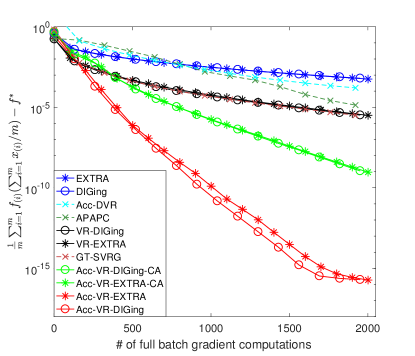
Refer to caption Refer to caption
Figure 1: Comparisons on Erdős-Rényi random graph with μ=5×10⁷𝜇5superscript107\mu=5\times 10^{-7} (top), μ=5×10⁶𝜇5superscript106\mu=5\times 10^{-6} (middle), and μ=5×10⁵𝜇5superscript105\mu=5\times 10^{-5} (bottom).
Refer to caption Refer to caption
Figure 2: Comparisons on grid graph with μ=5×10⁷𝜇5superscript107\mu=5\times 10^{-7} (top), μ=5×10⁶𝜇5superscript106\mu=5\times 10^{-6} (middle), and μ=5×10⁵𝜇5superscript105\mu=5\times 10^{-5} (bottom).

Figures 1 and 2 plot the results on the Erdős-Rényi random graph and grid graph, respectively, where fsuperscript𝑓f^{*} is approximated by the minimum value of the objective function over all iterations of all the compared algorithms. We have the following observations:

  1. 1.

    VR-EXTRA and VR-DIGing need less gradient computations than EXTRA and DIGing to reach the same precision for all cases of μ𝜇\mu. This verifies the efficiency of variance reduction in decentralized optimization to reduce the computation cost.

  2. 2.

    When considering the communication cost, VR-EXTRA and VR-DIGing perform worse than EXTRA and DIGing in practice, although they have the same communication complexities theoretically. This is reasonable since EXTRA and DIGing go through all the data at each communication round, while VR-EXTRA and VR-DIGing only use a mini-batch. We observe the mini-batch size of b=L¯fLf16𝑏subscript¯𝐿𝑓subscript𝐿𝑓16b=\frac{\overline{L}_{f}}{L_{f}}\approx 16 in our experiment.

  3. 3.

    Acc-VR-EXTRA and Acc-VR-DIGing perform better than VR-EXTRA and VR-DIGing on both computations and communications when κssubscript𝜅𝑠\kappa_{s} is much larger than n𝑛n. For example, κs=1000nsubscript𝜅𝑠1000𝑛\kappa_{s}=1000n in the top plots and κs=100nsubscript𝜅𝑠100𝑛\kappa_{s}=100n in the middle plots. Otherwise, as seen in the bottom plots with κs=10nsubscript𝜅𝑠10𝑛\kappa_{s}=10n, Acc-VR-EXTRA and Acc-VR-DIGing perform quite similarly to VR-EXTRA and VR-DIGing, especially on the computations. This verifies that acceleration only takes effect to reduce the computation cost when κsnmuch-greater-thansubscript𝜅𝑠𝑛\kappa_{s}\gg n.

  4. 4.

    When considering the communication cost, Acc-VR-EXTRA performs similarly to the optimal full batch method of APAPC. This observation matches the theory that the two methods have the same communication complexity.

  5. 5.

    Acc-VR-EXTRA-CA and Acc-VR-DIGing-CA do not perform well in practice, although they are theoretically optimal. Thus Acc-VR-EXTRA-CA and Acc-VR-DIGing-CA are more interesting in theory, but they are not suggested in practice.

6 Conclusion and Future Research

This paper extends the widely used EXTRA and DIGing methods with variance reduction, and four VR-based stochastic decentralized algorithms are proposed. The proposed VR-EXTRA has the 𝒪((κs+n)log1ϵ)𝒪subscript𝜅𝑠𝑛1italic-ϵ{\cal O}((\kappa_{s}+n)\log\frac{1}{\epsilon}) stochastic gradient computation complexity and the 𝒪((κb+κc)log1ϵ)𝒪subscript𝜅𝑏subscript𝜅𝑐1italic-ϵ{\cal O}((\kappa_{b}+\kappa_{c})\log\frac{1}{\epsilon}) communication complexity. The proposed VR-DIGing has a little worse communication complexity of 𝒪((κb+κc2)log1ϵ)𝒪subscript𝜅𝑏superscriptsubscript𝜅𝑐21italic-ϵ{\cal O}((\kappa_{b}+\kappa_{c}^{2})\log\frac{1}{\epsilon}). Our stochastic gradient computation complexities keep the same as the single-machine VR methods such as SVRG, and our communication complexities are the same as those of EXTRA and DIGing, respectively. The proposed accelerated VR-EXTRA and VR-DIGing achieve both the optimal 𝒪((nκs+n)log1ϵ)𝒪𝑛subscript𝜅𝑠𝑛1italic-ϵ{\cal O}((\sqrt{n\kappa_{s}}+n)\log\frac{1}{\epsilon}) stochastic gradient computation complexity and 𝒪(κbκclog1ϵ)𝒪subscript𝜅𝑏subscript𝜅𝑐1italic-ϵ{\cal O}(\sqrt{\kappa_{b}\kappa_{c}}\log\frac{1}{\epsilon}) communication complexity. They are also the same as the ones of single-machine accelerated VR methods such as Katyusha, and the accelerated full batch decentralized methods such as MSDA, respectively.

DIGing, called gradient tracking in other literatures, is a fundamental decentralized algorithm in the distributed optimization community. However, its state-of-the-art complexity is 𝒪((κb+κc2)log1ϵ)𝒪subscript𝜅𝑏superscriptsubscript𝜅𝑐21italic-ϵ{\cal O}((\kappa_{b}+\kappa_{c}^{2})\log\frac{1}{\epsilon}), which is worse than the 𝒪((κb+κc)log1ϵ)𝒪subscript𝜅𝑏subscript𝜅𝑐1italic-ϵ{\cal O}((\kappa_{b}+\kappa_{c})\log\frac{1}{\epsilon}) one of EXTRA. An open problem is that can we improve it from 𝒪((κb+κc2)log1ϵ)𝒪subscript𝜅𝑏superscriptsubscript𝜅𝑐21italic-ϵ{\cal O}((\kappa_{b}+\kappa_{c}^{2})\log\frac{1}{\epsilon}) to 𝒪((κb+κc)log1ϵ)𝒪subscript𝜅𝑏subscript𝜅𝑐1italic-ϵ{\cal O}((\kappa_{b}+\kappa_{c})\log\frac{1}{\epsilon})? Recently, Koloskova et al. (2021) gave some potential directions, where the complexity is improved from 𝒪(κb2κc2log1ϵ)𝒪superscriptsubscript𝜅𝑏2superscriptsubscript𝜅𝑐21italic-ϵ{\cal O}(\kappa_{b}^{2}\kappa_{c}^{2}\log\frac{1}{\epsilon}) (Qu & Li, 2018) to 𝒪(κbκclog1ϵ)𝒪subscript𝜅𝑏subscript𝜅𝑐1italic-ϵ{\cal O}(\kappa_{b}\kappa_{c}\log\frac{1}{\epsilon}). That is, the dependence on κc2superscriptsubscript𝜅𝑐2\kappa_{c}^{2} has been reduced to κcsubscript𝜅𝑐\kappa_{c}. Currently, it is unclear whether the complexity can be further improved to 𝒪((κb+κc)log1ϵ)𝒪subscript𝜅𝑏subscript𝜅𝑐1italic-ϵ{\cal O}((\kappa_{b}+\kappa_{c})\log\frac{1}{\epsilon}).

In our Algorithms 1 and 2, we set the parameters dependent on κcsubscript𝜅𝑐\kappa_{c}, Lfsubscript𝐿𝑓L_{f}, and L¯fsubscript¯𝐿𝑓\overline{L}_{f}, where κcsubscript𝜅𝑐\kappa_{c} needs the global knowledge of the network, while Lfsubscript𝐿𝑓L_{f} and L¯fsubscript¯𝐿𝑓\overline{L}_{f} needs to know the parameters of the other nodes. It is important to design practical algorithms only dependent on the local parameters, such as the Lipschitz constant L(i)subscript𝐿𝑖L_{(i)} and strong-convexity constant μ(i)subscript𝜇𝑖\mu_{(i)}, while still keep the optimal complexities. Another open problem is whether the reformulation (6) can be extended to directed graphs, where U𝑈U and V𝑉V cannot simply take the ones in this paper. Other interesting extensions include compression, asynchrony, and so on.

References

  • Alghunaim et al. (2021) Alghunaim, S. A., Ryu, E. K., Yuan, K., and H.Sayed, A. Decentralized proximal gradient algorithms with linear covnergence rates. IEEE Transactions on Automatic Control, 66(6):2787–2794, 2021.
  • Allen-Zhu (2018) Allen-Zhu, Z. Katyusha: The first direct acceleration of stochastic gradient methods. Journal of Machine Learning Research, 18(221):1–51, 2018.
  • Arioli & Scott (2014) Arioli, M. and Scott, J. Chebyshev acceleration of iterative refinement. Numerical Algorithms, 66(3):591–608, 2014.
  • Auzinger & Melenk (2017) Auzinger, W. and Melenk, J. M. Iterative solution of large linear systems. Lecture notes, TU Wien, 2017.
  • Aybat et al. (2018) Aybat, N. S., Wang, Z., Lin, T., and Ma, S. Distributed linearized alternating direction method of multipliers for composite convex consensus optimization. IEEE Transactions on Automatic Control, 63(1):5–20, 2018.
  • Bertsekas (1982) Bertsekas, D. P. Constrained Optimization and Lagrange Multiplier Methods. Athena Scientific, Belmont, Massachusetts, 1982.
  • Bertsekas (1983) Bertsekas, D. P. Distributed asynchromous computation of fixed points. Mathmatical Programming, 27:107–120, 1983.
  • Boyd et al. (2004) Boyd, S., Diaconis, P., and Xiao, L. Fastest mixing markov chain on a graph. SIAM Review, 46(4):667–689, 2004.
  • Chen & Sayed (2012) Chen, J. and Sayed, A. H. Diffusion adaptation strategies for distributed optimization and learning over networks. IEEE Transactions on Signal Processing, 60(8):4289–4305, 2012.
  • Defazio et al. (2014) Defazio, A., Bach, F., and Lacoste-Julien, S. SAGA: A fast incremental gradient method with support for non-strongly convex composite objectives. In Advances in Neural Information Processing Systems (NIPS), pp.  1646–1654, 2014.
  • Dvinskikh & Gasnikov (2021) Dvinskikh, D. and Gasnikov, A. Decentralized and parallelized primal and dual accelerated methods for stochastic convex programming problems. Journal of Inverse and Ill-posed Problems, 29(3):385–405, 2021.
  • Fallah et al. (2019) Fallah, A., Gürbüzbalaban, M., Ozdaglar, A., Simsekli, U., and Zhu, L. Robust distributed accelerated stochastic gradient methods for multi-agent networks. preprint arXiv:1910.08701, 2019.
  • Fercoq & Richtárik (2015) Fercoq, O. and Richtárik, P. Accelerated, parallel, and proximal coordinate descent. SIAM Journal on Optimization, 25(4):1997–2023, 2015.
  • Gorbunov et al. (2019) Gorbunov, E., Dvinskikh, D., and Gasnikov, A. Optimal decentralized distributed algorithms for stochastic convex optimization. preprint arXiv:1911.07363, 2019.
  • Gorbunov et al. (2022) Gorbunov, E., Rogozin, A., Beznosikov, A., Dvinskikh, D., and Gasnikov, A. Recent theoretical advances in decentralized distributed convex optimization. In High-Dimensional Optimization and Probability, pp. 253–325. Springer, 2022.
  • Hendrikx et al. (2020) Hendrikx, H., Bach, F., and Massoulié, L. Dual-free stochastic decentralized optimization with variance reduction. In Advances in Neural Information Processing Systems (NeurIPS), pp.  19455–19466, 2020.
  • Hendrikx et al. (2021) Hendrikx, H., Bach, F., and Massoulié, L. An optimal algorithm for decentralized finite-sum optimization. SIAM Journal on Optimization, 31(4):2753–2783, 2021.
  • Hong et al. (2017) Hong, M., Hajinezhad, D., and Zhao, M.-M. Prox-PDA: The proximal primal-dual algorithm for fast distributed nonconvex optimization and learning over networks. In International Conference on Machine Learning (ICML), pp. 1529–1538, 2017.
  • Iutzeler et al. (2016) Iutzeler, F., Bianchi, P., Ciblat, P., and Hachem, W. Explicit convergence rate of a distributed alternating direction method of multipliers. IEEE Transactions on Automatic Control, 61(4):892–904, 2016.
  • Jakovetić (2019) Jakovetić, D. A unification and generatliztion of exact distributed first order methods. IEEE Transactions on Signal and Information Processing over Networks, 5(1):31–46, 2019.
  • Jakovetić et al. (2014) Jakovetić, D., Xavier, J., and Moura, J. M. F. Fast distributed gradient methods. IEEE Transactions on Automatic Control, 59(5):1131–1146, 2014.
  • Johnson & Zhang (2013) Johnson, R. and Zhang, T. Accelerating stochastic gradient descent using predictive variance reduction. In Advances in Neural Information Processing Systems (NIPS), pp.  315–323, 2013.
  • Koloskova et al. (2021) Koloskova, A., Lin, T., and Stich, S. U. An improved analysis of gradient tracking for decentralized machine learning. In Advances in Neural Information Processing Systems (NeurIPS), pp.  11422–11435, 2021.
  • Kovalev et al. (2020a) Kovalev, D., Horváth, S., and Richtárik, P. Don’t jump through hoops and remove those loops: SVRG and Katyusha are better without the outer loop. In International Conference on Algorithmic Learning Theory (ALT), pp.  451–467, 2020a.
  • Kovalev et al. (2020b) Kovalev, D., Salim, A., and Richtárik, P. Optimal and practical algorithms for smooth and strongly convex decentralized optimization. In Advances in Neural Information Processing Systems (NeurIPS), pp.  18342–18352, 2020b.
  • Lan & Zhou (2018) Lan, G. and Zhou, Y. An optimal randomized incremental gradient method. Mathematical Programming, 171:167–215, 2018.
  • Lan et al. (2020) Lan, G., Lee, S., and Zhou, Y. Communication-efficient algorithms for decentralized and stochastic optimization. Mathematical Programming, 180:237–284, 2020.
  • Li et al. (2020a) Li, B., Cen, S., Chen, Y., and Chi, Y. Communication-efficient distributed optimization in networks with gradient tracking and variance reduction. Journal of Machine Learning Research, 21(180):1–51, 2020a.
  • Li & Lin (2020) Li, H. and Lin, Z. Revisiting EXTRA for smooth distributed optimization. SIAM Journal on Optimization, 30(3):1795–1821, 2020.
  • Li et al. (2020b) Li, H., Fang, C., Yin, W., and Lin, Z. Decentralized accelerated gradient methods with increasing penalty parameters. IEEE transactions on Signal Processing, 68:4855–4870, 2020b.
  • Li et al. (2019) Li, Z., Shi, W., and Yan, M. A decentralized proximal-gradient method with network independent step-sizes and separated convergence rates. IEEE Transactions on Signal Processing, 67(17):4494–4506, 2019.
  • Lin et al. (2018) Lin, H., Mairal, J., and Harchaoui, Z. Catalyst acceleration for first-order convex optimization: from theory to practice. Journal of Machine Learning Research, 18(212):1–54, 2018.
  • Lin et al. (2015) Lin, Q., Lu, Z., and Xiao, L. An accelerated randomized proximal coordinate gradient method and its application to regularized empirical risk minimization. SIAM Journal on Optimization, 25(4):2244–2273, 2015.
  • Makhdoumi & Ozdaglar (2017) Makhdoumi, A. and Ozdaglar, A. Convergence rate of distributed ADMM over networks. IEEE Transactions on Automatic Control, 62(10):5082–5095, 2017.
  • Mokhtari & Ribeiro (2016) Mokhtari, A. and Ribeiro, A. DSA: Decenrtalized double stochastic averaging gradient algorithm. Journal of Machine Learning Research, 17(61):1–35, 2016.
  • Nedić (2011) Nedić, A. Asynchronous broadcast-based convex optimization over a network. IEEE Transactions on Automatic Control, 56(6):1337–1351, 2011.
  • Nedić & Ozdaglar (2009) Nedić, A. and Ozdaglar, A. Distributed subgradient methods for multi-agent optimization. IEEE Transactions on Automatic Control, 54(1):48–61, 2009.
  • Nedić et al. (2017) Nedić, A., Olshevsky, A., and Shi, W. Achieving geometric convergence for distributed optimization over time-varying graphs. SIAM Journal on Optimization, 27(4):2597–2633, 2017.
  • Nedić et al. (2018) Nedić, A., Olshevsky, A., and Rabbat, M. G. Network topology and communication-computation tradeoffs in decentralized optimization. Proceedings of the IEEE, 106(5):953–976, 2018.
  • Nesterov (2004) Nesterov, Y. Introductory Lectures on Convex Optimization: A Basic Course. Kluwer Academic, Boston, 2004.
  • Pu & Nedić (2021) Pu, S. and Nedić, A. Distributed stochastic gradient tracking methods. Mathematical Programming, 187:409–457, 2021.
  • Qu & Li (2018) Qu, G. and Li, N. Harnessing smoothness to accelerate distributed optimization. IEEE Transactions on Control of Network Systems, 5(3):1245–1260, 2018.
  • Qu & Li (2020) Qu, G. and Li, N. Accelerated distributed Nesterov gradient descent. IEEE Transactions on Automatic Control, 65(6):2566–2581, 2020.
  • Ram et al. (2010) Ram, S. S., Nedić, A., and Veeravalli, V. V. Distributed stochastic subgradient projection algorithms for convex optimization. Journal of Optimization Theory and Applications, 147:516–545, 2010.
  • Scaman et al. (2017) Scaman, K., Bach, F., Bubeck, S., Lee, Y. T., and Massoulié, L. Optimal algorithms for smooth and strongly convex distributed optimization in networks. In International Conference on Machine Learning (ICML), pp. 3027–3036, 2017.
  • Scaman et al. (2018) Scaman, K., Bach, F., Bubeck, S., Lee, Y. T., and Massoulié, L. Optimal algorithms for non-smooth distributed optimization in networks. In Advances in Neural Information Processing Systems (NeurIPS), pp.  2740–2749, 2018.
  • Scaman et al. (2019) Scaman, K., Bach, F., Bubeck, S., Lee, Y. T., and Massoulié, L. Optimal convergence rates for convex distributed optimization in networks. Journal of Machine Learning Research, 20(159):1–31, 2019.
  • Schmidt et al. (2017) Schmidt, M., Le Roux, N., and Bach, F. Minimizing finite sums with the stochastic average gradient. Mathematical Programming, 162:83–112, 2017.
  • Shi et al. (2015) Shi, W., Ling, Q., Wu, G., and Yin, W. EXTRA: An exact first-order algorithm for decentralized consensus optimization. SIAM Journal on Optimization, 25(2):944–966, 2015.
  • Terelius et al. (2011) Terelius, H., Topcu, U., and Murray, R. M. Decentralized multi-agent optimization via dual decomposition. IFAC proceedings volumes, 44(1):11245–11251, 2011.
  • Tsitsiklis et al. (1986) Tsitsiklis, J. N., Bertsekas, D. P., and Athans, M. Distributed asynchronous deterministic and stochastic gradient optimization algorithms. IEEE Transaction on Automatic Control, 31(9):803–812, 1986.
  • Uribe et al. (2020) Uribe, C. A., Lee, S., Gasnikov, A., and Nedić, A. A dual approach for optimal algorithms in distributed optimization over networks. In Information Theory and Applications Workshop (ITA), pp. 1–37, 2020.
  • Xiao & Zhang (2014) Xiao, L. and Zhang, T. A proximal stochastic gradient method with progressive variance reduction. SIAM Journal on Optimization, 24(4):2057–2075, 2014.
  • Xin et al. (2018) Xin, R., Khan, U. A., and Kar, S. A linear algorithm for optimization over directed graphs with geometric convergence. IEEE Control Systems Letters, 2(3):315–320, 2018.
  • Xin et al. (2020a) Xin, R., Kar, S., and Khan, U. A. Decentralized stochastic optimization and machine learning: A unified variance-reduction framework for robust performance and fast convergence. IEEE Signal Processing Magazine, 37(3):102–113, 2020a.
  • Xin et al. (2020b) Xin, R., Khan, U. A., and Kar, S. Variance-reduced decentralized stochastic optimization with accelerated convergence. IEEE Transactions on Signal Processing, 68:6255–6271, 2020b.
  • Xu et al. (2015) Xu, J., Zhu, S., Soh, Y. C., and Xie, L. Augmented distributed gradient methods for multi-agent optimization under uncoordinated constant stepsizes. In IEEE Conference on Decision and Control (CDC), pp. 2055–2060, 2015.
  • Yuan et al. (2016) Yuan, K., Ling, Q., and Yin, W. On the convergence of decentralized gradient descent. SIAM Journal on Optimization, 26(3):1835–1854, 2016.
  • Zhou et al. (2019) Zhou, K., Shang, F., and Cheng, J. A simple stochastic variance reduced algorithm with fast convergence rates. In International Conference on Machine Learning (ICML), pp. 5975–5984, 2019.