Minimum variance estimation of statistical anisotropy via galaxy survey

Maresuke Shiraishi    Teppei Okumura    and Kazuyuki Akitsu
Abstract

We consider the benefits of measuring cosmic statistical anisotropy from redshift-space correlators of the galaxy number density fluctuation and the peculiar velocity field without adopting the plane-parallel (PP) approximation. Since the correlators are decomposed using the general tripolar spherical harmonic (TripoSH) basis, we can deal with wide-angle contributions untreatable by the PP approximation, and at the same time, target anisotropic signatures can be cleanly extracted. We, for the first time, compute the covariance of the TripoSH decomposition coefficient and the Fisher matrix to forecast the detectability of statistical anisotropy. The resultant expression of the covariance is free from nontrivial mixings between each multipole moment caused by the PP approximation and hence the detectability is fully optimized. Compared with the analysis under the PP approximation, the superiority in detectability is always confirmed, and it is highlighted, especially in the cases that the shot noise level is large and that target statistical anisotropy has a blue-tilted shape in Fourier space. The application of the TripoSH-based analysis to forthcoming all-sky survey data could result in constraints on anisotropy comparable to or tighter than the current cosmic microwave background ones.

1 Introduction

The assumption of global isotropy of the Universe is one key underpinning of the concordance ΛΛ\LambdaCDM cosmology. This is linked with the cosmic no-hair conjecture at the primordial inflationary stage. On the other hand, recently, possibilities of the departure from isotropy have been widely and thoroughly argued. The presence of some source fields as vector or higher-spin fields (e.g. [1, 2, 3, 4]), an inflating solid (e.g. [5, 6]), fossil gravitational waves (e.g. [7, 8]) and large-scale tides (e.g. [9, 10, 11, 12, 13]) in both early and late Universe has been proposed and studied for such possibilities.

Broken isotropy or equivalently broken rotational invariance imprints quite unique signatures in the two-point correlation function (2PCF) or the power spectrum between a variety of cosmic observables such as the cosmic microwave background (CMB), large-scale structure, the 21-cm radiation and the gravitational wave background. The anisotropic signatures have been tested with diverse observed data, however, there is no detection up to now. In the analysis using angular power spectra computed on the 2D sphere, a nonvanishing signal in off-diagonal multipole modes is an observational indicator. No detection of it places upper bound on the anisotropic component. The stringent one comes from the CMB, reading 102similar-toabsentsuperscript102\sim 10^{-2} of the isotropic component [14, 15, 16, 17]. Such constraints can be utilized for determining the particle content of the Universe (e.g. [18, 19, 20]).

On the other hand, very recently, the isotropy test in the 3D space has also been thoroughly examined. In ref. [21], we developed an efficient way to extract the anisotropic signal from the 2PCF of 3D galaxy clustering. The current upper bound obtained in this way is within an order of magnitude of the CMB constraint [22], while a drastic update is expected in the future since the signal-to-noise ratio in the 3D analysis grows even faster than the 2D one as the number of accessible Fourier modes increases [21, 19, 13].

The observational constraints and their forecasts mentioned above were obtained imposing the plane-parallel (PP) approximation where two different line-of-sight (LOS) directions s^1subscript^𝑠1\hat{s}_{1} and s^2subscript^𝑠2\hat{s}_{2} are identified with each other. This approximation has worked well in the analysis of galaxy surveys so far because the data where the visible angle of the survey area become too large has not been used. In contrast, this approximation is not applicable to the analysis including any wide-angle contribution targeted by proposed all-sky surveys such as SPHEREx [23], Euclid [24] and WFIRST [25]. Establishing a complete analysis methodology without the PP approximation is therefore a pressing issue.111See refs. [26, 27, 28] for a few studies on analyzing observed galaxy clustering in configuration space.

In the absence of the PP approximation, the 2PCF is characterized by three directions: two LOS vectors, s^1subscript^𝑠1\hat{s}_{1} and s^2subscript^𝑠2\hat{s}_{2}, and its separation vector, s^12𝐬1𝐬2^subscript^𝑠12^subscript𝐬1subscript𝐬2\hat{s}_{12}\equiv\widehat{{\bf s}_{1}-{\bf s}_{2}}, where hat denotes a unit vector. In the appendix of ref. [21], we found that the directional dependence can be completely decomposed using the general tripolar spherical harmonic (TripoSH) basis {Y(s^12){Y1(s^1)Y2(s^2)}}LMsubscripttensor-productsubscript𝑌subscript^𝑠12subscripttensor-productsubscript𝑌subscript1subscript^𝑠1subscript𝑌subscript2subscript^𝑠2superscript𝐿𝑀\{Y_{\ell}(\hat{s}_{12})\otimes\{Y_{\ell_{1}}(\hat{s}_{1})\otimes Y_{\ell_{2}}(\hat{s}_{2})\}_{\ell^{\prime}}\}_{LM} [29]. If the Universe is isotropic, nonvanishing coefficients are confined to L=0𝐿0L=0. There are many previous works on the response of the L=0𝐿0L=0 coefficients on a variety of isotropic Universe models (e.g. [30, 31, 32, 33, 34, 35]).222See e.g., refs. [36, 37, 38, 39, 40] for other decomposition approaches. In contrast, ref. [21] showed that the L>0𝐿0L>0 coefficients become a clean indicator of broken isotropy.

As for L=0𝐿0L=0, very recently, the covariance of the TripoSH coefficient was also examined in our paper [41]. We then found that nontrivial mixings between different multipole moments as seen in the PP-limit covariance do not exist. This fact minimizes the covariance and hence drastically optimizes the signal-to-noise ratio, especially at higher multipole moments.

In this paper, in anticipation of the anisotropic signal measurement using wide-angle data, we generalize our covariance formalism in ref. [41] by including L>0𝐿0L>0. As in ref. [41], we consider power spectra of density and velocity fields in redshift space as observables in galaxy redshift surveys, peculiar velocity surveys and kinematic Sunyaev-Zel’dovich surveys (e.g. [42, 43, 44, 45, 46, 47, 48, 49]). We then confirm that, even for L>0𝐿0L>0, the covariance is minimized by virtue of high separability of the general TripoSH basis. We also compute the Fisher matrix and forecast the constraints on a widely-used isotropy breaking parameter gLMsubscript𝑔𝐿𝑀g_{LM} [see eqs. (3.9) and (4.1) for definition] from the galaxy density and velocity fields. It is then found that our new TripoSH-based analysis always surpasses the previous PP-limit one in detectability of gLMsubscript𝑔𝐿𝑀g_{LM} thanks to minimizing the covariance, and the superiority becomes remarkable if the shot noise level enlarges or if target anisotropy has a blue-tilted shape in Fourier space.

This paper is organized as follows. In the next section, we summarize the linear-order expressions of the galaxy number density fluctuation and the peculiar velocity field underlying our discussions. In section 3, we perform the TripoSH decomposition of the 2PCF of the density and velocity fields and estimate the signal arising from the anisotropic Universe models and the covariance of the TripoSH coefficient. The error estimation on gLMsubscript𝑔𝐿𝑀g_{LM} is done in section 4. The final section is devoted to the conclusion of this paper. In appendix A, the Fisher matrix computation in the PP limit based on the bipolar spherical harmonic (BipoSH) decomposition is argued. In appendix B, some mathematical identities utilized in this paper are summarized.

2 Linear theory for cosmic density and velocity fields

In this paper, as cosmic observables, we take into account two scalar quantities: the galaxy number density contrast δ(𝐬)n(𝐬)/n¯(s)1𝛿𝐬𝑛𝐬¯𝑛𝑠1\delta({\bf s})\equiv n({\bf s})/\bar{n}(s)-1 and the LOS peculiar velocity field u(𝐬)=𝐯(𝐬)s^𝑢𝐬𝐯𝐬^𝑠u({\bf s})={\bf v}({\bf s})\cdot\hat{s} in redshift space. Since our main interest is to extract large-scale information on statistical anisotropy from galaxy clustering, we may work with the linear theory representation [50, 45, 34]:

X(𝐬)=d3k(2π)3ei𝐤𝐬FX(𝐤,s^),𝑋𝐬superscript𝑑3𝑘superscript2𝜋3superscript𝑒𝑖𝐤𝐬superscript𝐹𝑋𝐤^𝑠X({\bf s})=\int\frac{d^{3}k}{(2\pi)^{3}}e^{i{\bf k}\cdot{\bf s}}F^{X}({\bf k},\hat{s}), (2.1)

where X={δ,u}𝑋𝛿𝑢X=\{\delta,u\} and

Fδ(𝐤,s^)[biαks(k^s^)f+(k^s^)2f]δm(𝐤),Fu(𝐤,s^)iaHk(k^s^)fδm(𝐤).formulae-sequencesuperscript𝐹𝛿𝐤^𝑠delimited-[]𝑏𝑖𝛼𝑘𝑠^𝑘^𝑠𝑓superscript^𝑘^𝑠2𝑓subscript𝛿𝑚𝐤superscript𝐹𝑢𝐤^𝑠𝑖𝑎𝐻𝑘^𝑘^𝑠𝑓subscript𝛿𝑚𝐤\displaystyle\begin{split}F^{\delta}({\bf k},\hat{s})&\equiv\left[b-i\frac{\alpha}{ks}(\hat{k}\cdot\hat{s})f+(\hat{k}\cdot\hat{s})^{2}f\right]\delta_{m}({\bf k}),\\ F^{u}({\bf k},\hat{s})&\equiv i\frac{aH}{k}(\hat{k}\cdot\hat{s})f\delta_{m}({\bf k}).\end{split} (2.2)

The linear bias parameter b𝑏b, the linear growth rate f𝑓f, the scale factor a𝑎a, the Hubble parameter H𝐻H, the selection function αdlnn¯(s)/dlns+2𝛼𝑑¯𝑛𝑠𝑑𝑠2\alpha\equiv d\ln\bar{n}(s)/d\ln s+2, the real-space matter density fluctuation δm(𝐤)subscript𝛿𝑚𝐤\delta_{m}({\bf k}) and FX(𝐤,s^)superscript𝐹𝑋𝐤^𝑠F^{X}({\bf k},\hat{s}) depend on time, redshift or the conformal distance although it is not clearly stated as an argument for notational convenience. This convention is also adopted henceforth unless the parameter dependence is nontrivial. Note that FX(𝐤,s^)superscript𝐹𝑋𝐤^𝑠F^{X}({\bf k},\hat{s}) does not correspond to the Fourier counterpart of X(𝐬)𝑋𝐬X({\bf s}) because there still remains the s^^𝑠\hat{s} dependence. For later convenience, we expand the angular dependence due to the redshift-space distortion using the Legendre polynomials (x)subscript𝑥{\cal L}_{\ell}(x) as

FX(𝐤,s^)=jcjX(k)j(k^s^)δm(𝐤),superscript𝐹𝑋𝐤^𝑠subscript𝑗superscriptsubscript𝑐𝑗𝑋𝑘subscript𝑗^𝑘^𝑠subscript𝛿𝑚𝐤F^{X}({\bf k},\hat{s})=\sum_{j}c_{j}^{X}(k){\cal L}_{j}(\hat{k}\cdot\hat{s})\delta_{m}({\bf k}), (2.3)

where cjX=(1)jcjXsuperscriptsubscript𝑐𝑗𝑋superscript1𝑗superscriptsubscript𝑐𝑗𝑋c_{j}^{X*}=(-1)^{j}c_{j}^{X} and

c0δ=b+13f,c1δ=iαksf,c2δ=23f,cj3δ=0,c1u=iaHkf,c0u=cj2u=0.\displaystyle\begin{split}&c_{0}^{\delta}=b+\frac{1}{3}f,\ \ c_{1}^{\delta}=-i\frac{\alpha}{ks}f,\ \ c_{2}^{\delta}=\frac{2}{3}f,\ \ c_{j\geq 3}^{\delta}=0,\\ &c_{1}^{u}=i\frac{aH}{k}f,\ \ c_{0}^{u}=c_{j\geq 2}^{u}=0.\end{split} (2.4)

Now, we assume that the matter distribution in real space is statistically homogeneous but is allowed to be statistically anisotropic in anticipation of anisotropic cosmological scenarios. The matter power spectrum then takes the form

δm(𝐤1)δm(𝐤2)=(2π)3δ(3)(𝐤1+𝐤2)Pm(𝐤1).expectationsubscript𝛿𝑚subscript𝐤1subscript𝛿𝑚subscript𝐤2superscript2𝜋3superscript𝛿3subscript𝐤1subscript𝐤2subscript𝑃𝑚subscript𝐤1\Braket{\delta_{m}({\bf k}_{1})\delta_{m}({\bf k}_{2})}=(2\pi)^{3}\delta^{(3)}({\bf k}_{1}+{\bf k}_{2})P_{m}({\bf k}_{1}). (2.5)

In this case, the 2PCF of the density and velocity fields is written as

ξX1X2(𝐬12,s^1,s^2)superscript𝜉subscript𝑋1subscript𝑋2subscript𝐬12subscript^𝑠1subscript^𝑠2\displaystyle\xi^{X_{1}X_{2}}({\bf s}_{12},\hat{s}_{1},\hat{s}_{2}) \displaystyle\equiv X1(𝐬1)X2(𝐬2)expectationsubscript𝑋1subscript𝐬1subscript𝑋2subscript𝐬2\displaystyle\Braket{X_{1}({\bf s}_{1})X_{2}({\bf s}_{2})} (2.6)
=\displaystyle= d3k(2π)3ei𝐤𝐬12PX1X2(𝐤,s^1,s^2),superscript𝑑3𝑘superscript2𝜋3superscript𝑒𝑖𝐤subscript𝐬12superscript𝑃subscript𝑋1subscript𝑋2𝐤subscript^𝑠1subscript^𝑠2\displaystyle\int\frac{d^{3}k}{(2\pi)^{3}}e^{i{\bf k}\cdot{\bf s}_{12}}P^{X_{1}X_{2}}({\bf k},\hat{s}_{1},\hat{s}_{2}),

where 𝐬12𝐬1𝐬2subscript𝐬12subscript𝐬1subscript𝐬2{\bf s}_{12}\equiv{\bf s}_{1}-{\bf s}_{2} and

PX1X2(𝐤,s^1,s^2)=j1j2cj1X1(k)(1)j2cj2X2(k)j1(k^s^1)j2(k^s^2)Pm(𝐤).superscript𝑃subscript𝑋1subscript𝑋2𝐤subscript^𝑠1subscript^𝑠2subscriptsubscript𝑗1subscript𝑗2superscriptsubscript𝑐subscript𝑗1subscript𝑋1𝑘superscript1subscript𝑗2superscriptsubscript𝑐subscript𝑗2subscript𝑋2𝑘subscriptsubscript𝑗1^𝑘subscript^𝑠1subscriptsubscript𝑗2^𝑘subscript^𝑠2subscript𝑃𝑚𝐤P^{X_{1}X_{2}}({\bf k},\hat{s}_{1},\hat{s}_{2})=\sum_{j_{1}j_{2}}c_{j_{1}}^{X_{1}}(k)(-1)^{j_{2}}c_{j_{2}}^{X_{2}}(k){\cal L}_{j_{1}}(\hat{k}\cdot\hat{s}_{1}){\cal L}_{j_{2}}(\hat{k}\cdot\hat{s}_{2})P_{m}({\bf k}). (2.7)

Note that PX1X2(𝐤,s^1,s^2)superscript𝑃subscript𝑋1subscript𝑋2𝐤subscript^𝑠1subscript^𝑠2P^{X_{1}X_{2}}({\bf k},\hat{s}_{1},\hat{s}_{2}) cannot be regarded as the Fourier counterpart of ξX1X2(𝐬12,s^1,s^2)superscript𝜉subscript𝑋1subscript𝑋2subscript𝐬12subscript^𝑠1subscript^𝑠2\xi^{X_{1}X_{2}}({\bf s}_{12},\hat{s}_{1},\hat{s}_{2}) because the s^1subscript^𝑠1\hat{s}_{1} and s^2subscript^𝑠2\hat{s}_{2} dependence still leaves.

Our formalism developed below is based on these formulae. Although the contributions of unequal-time correlators are not included for simplicity, they become treatable through a small extension. The above variables depend on cosmological parameters. Our numerical analysis performed below is done by fixing their values to be consistent with the latest CMB limits [51].

3 Tripolar spherical harmonic decomposition

In this section, we decompose the 2PCF (2.6) using the TripoSH basis, and extract the anisotropic signatures. Moreover, we compute the covariance of the decomposition coefficient.

3.1 Decomposition rule

As seen in eq. (2.6), the 2PCF is characterized by s^12subscript^𝑠12\hat{s}_{12}, s^1subscript^𝑠1\hat{s}_{1} and s^2subscript^𝑠2\hat{s}_{2}. For a general angular decomposition basis, let us introduce the TripoSH function taking these three angles as arguments [29, 21]:

𝒳12LM(s^12,s^1,s^2)superscriptsubscript𝒳subscript1subscript2superscript𝐿𝑀subscript^𝑠12subscript^𝑠1subscript^𝑠2\displaystyle{\cal X}_{\ell\ell_{1}\ell_{2}\ell^{\prime}}^{LM}(\hat{s}_{12},\hat{s}_{1},\hat{s}_{2}) \displaystyle\equiv {Y(s^12){Y1(s^1)Y2(s^2)}}LMsubscripttensor-productsubscript𝑌subscript^𝑠12subscripttensor-productsubscript𝑌subscript1subscript^𝑠1subscript𝑌subscript2subscript^𝑠2superscript𝐿𝑀\displaystyle\{Y_{\ell}(\hat{s}_{12})\otimes\{Y_{\ell_{1}}(\hat{s}_{1})\otimes Y_{\ell_{2}}(\hat{s}_{2})\}_{\ell^{\prime}}\}_{LM} (3.1)
=\displaystyle= mm1m2m𝒞mmLM𝒞1m12m2mYm(s^12)Y1m1(s^1)Y2m2(s^2),subscript𝑚subscript𝑚1subscript𝑚2superscript𝑚superscriptsubscript𝒞𝑚superscriptsuperscript𝑚𝐿𝑀superscriptsubscript𝒞subscript1subscript𝑚1subscript2subscript𝑚2superscriptsuperscript𝑚subscript𝑌𝑚subscript^𝑠12subscript𝑌subscript1subscript𝑚1subscript^𝑠1subscript𝑌subscript2subscript𝑚2subscript^𝑠2\displaystyle\sum_{mm_{1}m_{2}m^{\prime}}{\cal C}_{\ell m\ell^{\prime}m^{\prime}}^{LM}{\cal C}_{\ell_{1}m_{1}\ell_{2}m_{2}}^{\ell^{\prime}m^{\prime}}Y_{\ell m}(\hat{s}_{12})Y_{\ell_{1}m_{1}}(\hat{s}_{1})Y_{\ell_{2}m_{2}}(\hat{s}_{2}),

where 𝒞l1m1l2m2l3m3(1)l1l2+m32l3+1(l1l2l3m1m2m3)superscriptsubscript𝒞subscript𝑙1subscript𝑚1subscript𝑙2subscript𝑚2subscript𝑙3subscript𝑚3superscript1subscript𝑙1subscript𝑙2subscript𝑚32subscript𝑙31matrixsubscript𝑙1subscript𝑙2subscript𝑙3subscript𝑚1subscript𝑚2subscript𝑚3{\cal C}_{l_{1}m_{1}l_{2}m_{2}}^{l_{3}m_{3}}\equiv(-1)^{l_{1}-l_{2}+m_{3}}\sqrt{2l_{3}+1}\left(\begin{matrix}l_{1}&l_{2}&l_{3}\\ m_{1}&m_{2}&-m_{3}\end{matrix}\right) is the Clebsch-Gordan coefficient. We decompose the 2PCF according to

ξX1X2(𝐬12,s^1,s^2)=12LMΞ12LMX1X2(s12)𝒳12LM(s^12,s^1,s^2).superscript𝜉subscript𝑋1subscript𝑋2subscript𝐬12subscript^𝑠1subscript^𝑠2subscriptsubscript1subscript2superscript𝐿𝑀superscriptsubscriptΞsubscript1subscript2superscript𝐿𝑀subscript𝑋1subscript𝑋2subscript𝑠12superscriptsubscript𝒳subscript1subscript2superscript𝐿𝑀subscript^𝑠12subscript^𝑠1subscript^𝑠2\xi^{X_{1}X_{2}}({\bf s}_{12},\hat{s}_{1},\hat{s}_{2})=\sum_{\ell\ell_{1}\ell_{2}\ell^{\prime}LM}\Xi_{\ell\ell_{1}\ell_{2}\ell^{\prime}}^{LMX_{1}X_{2}}(s_{12}){\cal X}_{\ell\ell_{1}\ell_{2}\ell^{\prime}}^{LM}(\hat{s}_{12},\hat{s}_{1},\hat{s}_{2}). (3.2)

Note that the coefficient with L=M=0𝐿𝑀0L=M=0, Ξ1200X1X2superscriptsubscriptΞsubscript1subscript200subscript𝑋1subscript𝑋2\Xi_{\ell\ell_{1}\ell_{2}\ell}^{00X_{1}X_{2}}, is equivalent to Ξ12X1X2superscriptsubscriptΞsubscript1subscript2subscript𝑋1subscript𝑋2\Xi_{\ell\ell_{1}\ell_{2}}^{X_{1}X_{2}} in ref. [41]. As confirmed in ref. [21] and the next subsection of this paper, distinctive signatures of statistical anisotropy appear for L>0𝐿0L>0.

Now, we consider the TripoSH decomposition of eq. (2.6). For later convenience, let us expand PX1X2superscript𝑃subscript𝑋1subscript𝑋2P^{X_{1}X_{2}} according to

PX1X2(𝐤,s^1,s^2)=12LMΠ12LMX1X2(k)𝒳12LM(k^,s^1,s^2).superscript𝑃subscript𝑋1subscript𝑋2𝐤subscript^𝑠1subscript^𝑠2subscriptsubscript1subscript2superscript𝐿𝑀superscriptsubscriptΠsubscript1subscript2superscript𝐿𝑀subscript𝑋1subscript𝑋2𝑘superscriptsubscript𝒳subscript1subscript2superscript𝐿𝑀^𝑘subscript^𝑠1subscript^𝑠2P^{X_{1}X_{2}}({\bf k},\hat{s}_{1},\hat{s}_{2})=\sum_{\ell\ell_{1}\ell_{2}\ell^{\prime}LM}\Pi_{\ell\ell_{1}\ell_{2}\ell^{\prime}}^{LMX_{1}X_{2}}(k){\cal X}_{\ell\ell_{1}\ell_{2}\ell^{\prime}}^{LM}(\hat{k},\hat{s}_{1},\hat{s}_{2}). (3.3)

Plugging this into eq. (2.6) and simplifying the k^^𝑘\hat{k} integral by use of eqs. (B.1) and (B.2), we find that ξX1X2superscript𝜉subscript𝑋1subscript𝑋2\xi^{X_{1}X_{2}} recovers eq. (3.2) with

Ξ12LMX1X2(s12)=i0k2dk2π2j(ks12)Π12LMX1X2(k).superscriptsubscriptΞsubscript1subscript2superscript𝐿𝑀subscript𝑋1subscript𝑋2subscript𝑠12superscript𝑖superscriptsubscript0superscript𝑘2𝑑𝑘2superscript𝜋2subscript𝑗𝑘subscript𝑠12superscriptsubscriptΠsubscript1subscript2superscript𝐿𝑀subscript𝑋1subscript𝑋2𝑘\Xi_{\ell\ell_{1}\ell_{2}\ell^{\prime}}^{LMX_{1}X_{2}}(s_{12})=i^{\ell}\int_{0}^{\infty}\frac{k^{2}dk}{2\pi^{2}}j_{\ell}(ks_{12})\Pi_{\ell\ell_{1}\ell_{2}\ell^{\prime}}^{LMX_{1}X_{2}}(k). (3.4)

The practical form of Π12LMX1X2superscriptsubscriptΠsubscript1subscript2superscript𝐿𝑀subscript𝑋1subscript𝑋2\Pi_{\ell\ell_{1}\ell_{2}\ell^{\prime}}^{LMX_{1}X_{2}} is obtained computing

Π12LMX1X2(k)=d2k^d2s^1d2s^2PX1X2(𝐤,s^1,s^2)𝒳12LM(k^,s^1,s^2).superscriptsubscriptΠsubscript1subscript2superscript𝐿𝑀subscript𝑋1subscript𝑋2𝑘superscript𝑑2^𝑘superscript𝑑2subscript^𝑠1superscript𝑑2subscript^𝑠2superscript𝑃subscript𝑋1subscript𝑋2𝐤subscript^𝑠1subscript^𝑠2superscriptsubscript𝒳subscript1subscript2superscript𝐿𝑀^𝑘subscript^𝑠1subscript^𝑠2\Pi_{\ell\ell_{1}\ell_{2}\ell^{\prime}}^{LMX_{1}X_{2}}(k)=\int d^{2}\hat{k}\int d^{2}\hat{s}_{1}\int d^{2}\hat{s}_{2}\,P^{X_{1}X_{2}}({\bf k},\hat{s}_{1},\hat{s}_{2}){\cal X}_{\ell\ell_{1}\ell_{2}\ell^{\prime}}^{LM*}(\hat{k},\hat{s}_{1},\hat{s}_{2}). (3.5)

It is convenient to introduce a reduced coefficient:

𝒫12LMX1X2(k)(1)L+h12hL4π(2+1)Π12LMX1X2(k),superscriptsubscript𝒫subscript1subscript2superscript𝐿𝑀subscript𝑋1subscript𝑋2𝑘superscript1𝐿superscriptsubscriptsubscript1subscript2superscriptsubscriptsuperscript𝐿4𝜋2superscript1superscriptsubscriptΠsubscript1subscript2superscript𝐿𝑀subscript𝑋1subscript𝑋2𝑘{\cal P}_{\ell\ell_{1}\ell_{2}\ell^{\prime}}^{LMX_{1}X_{2}}(k)\equiv(-1)^{L+\ell^{\prime}}\frac{h_{\ell_{1}\ell_{2}\ell^{\prime}}h_{\ell\ell^{\prime}L}}{\sqrt{4\pi(2\ell^{\prime}+1)}}\Pi_{\ell\ell_{1}\ell_{2}\ell^{\prime}}^{LMX_{1}X_{2}}(k), (3.6)

where

hl1l2l3(2l1+1)(2l2+1)(2l3+1)4π(l1l2l3000).subscriptsubscript𝑙1subscript𝑙2subscript𝑙32subscript𝑙112subscript𝑙212subscript𝑙314𝜋matrixsubscript𝑙1subscript𝑙2subscript𝑙3000h_{l_{1}l_{2}l_{3}}\equiv\sqrt{\frac{(2l_{1}+1)(2l_{2}+1)(2l_{3}+1)}{4\pi}}\left(\begin{matrix}l_{1}&l_{2}&l_{3}\\ 0&0&0\end{matrix}\right). (3.7)

The coefficient 𝒫12LMX1X2superscriptsubscript𝒫subscript1subscript2superscript𝐿𝑀subscript𝑋1subscript𝑋2{\cal P}_{\ell\ell_{1}\ell_{2}\ell^{\prime}}^{LMX_{1}X_{2}} corresponds to the BipoSH coefficient in the PP limit s^1=s^2subscript^𝑠1subscript^𝑠2\hat{s}_{1}=\hat{s}_{2} (see appendix A.1 for definition) with a simple relation:

PLMX1X2(k)=12𝒫12LMX1X2(k);superscriptsubscript𝑃superscript𝐿𝑀subscript𝑋1subscript𝑋2𝑘subscriptsubscript1subscript2superscriptsubscript𝒫subscript1subscript2superscript𝐿𝑀subscript𝑋1subscript𝑋2𝑘P_{\ell\ell^{\prime}}^{LMX_{1}X_{2}}(k)=\sum_{\ell_{1}\ell_{2}}{\cal P}_{\ell\ell_{1}\ell_{2}\ell^{\prime}}^{LMX_{1}X_{2}}(k); (3.8)

thus, facilitates the comparison with the previous PP-limit results. One can see from this that, in the PP approximation, the two multipole moments 1subscript1\ell_{1} and 2subscript2\ell_{2}, which are associated with s^1subscript^𝑠1\hat{s}_{1} and s^2subscript^𝑠2\hat{s}_{2}, respectively, are contracted and disappear. This gives rise to the information loss (see appendix A.3 for details).

3.2 Anisotropic signal

If the matter distribution in real space breaks statistical isotropy, there remains k^^𝑘\hat{k} dependence in its power spectrum. We express it with a generic form,

Pm(𝐤)=P¯m(k)LMGLM(k)YLM(k^),subscript𝑃𝑚𝐤subscript¯𝑃𝑚𝑘subscript𝐿𝑀subscript𝐺𝐿𝑀𝑘subscript𝑌𝐿𝑀^𝑘P_{m}({\bf k})=\bar{P}_{m}(k)\sum_{LM}G_{LM}(k)Y_{LM}(\hat{k}), (3.9)

where P¯msubscript¯𝑃𝑚\bar{P}_{m}\in\mathbb{R} quantifies the isotropic component (and hence G00=4πsubscript𝐺004𝜋G_{00}=\sqrt{4\pi}), and GL1,M(k)subscript𝐺𝐿1𝑀𝑘G_{L\geq 1,M}(k) represents the fraction of the departure from isotropy, obeying GLM=(1)MGL,Msubscript𝐺𝐿𝑀superscript1𝑀superscriptsubscript𝐺𝐿𝑀G_{LM}=(-1)^{M}G_{L,-M}^{*}\in\mathbb{C} and GL=odd,M=0subscript𝐺𝐿odd𝑀0G_{L={\rm odd},M}=0 from Pm(𝐤)=Pm(𝐤)=Pm(𝐤)subscript𝑃𝑚𝐤subscript𝑃𝑚𝐤superscriptsubscript𝑃𝑚𝐤P_{m}({\bf k})=P_{m}(-{\bf k})=P_{m}^{*}(-{\bf k}). This type of directional dependence can originate from the primordial curvature power spectrum, e.g., if higher spin fields couple to some scalar fields in the inflationary era. In the simplest case where there are spin-1 vectors coupled to inflaton scalars, G2Msubscript𝐺2𝑀G_{2M} does not vanish as well as G00subscript𝐺00G_{00} (e.g. [52, 53, 54, 55, 56, 18, 57]). More generally, spin-s𝑠s fields generate G00subscript𝐺00G_{00}, G2Msubscript𝐺2𝑀G_{2M}, G4Msubscript𝐺4𝑀G_{4M}, \cdots, G2(s1),Msubscript𝐺2𝑠1𝑀G_{2(s-1),M} and G2s,Msubscript𝐺2𝑠𝑀G_{2s,M} [4, 19]. Nonvanishing GL>2,Msubscript𝐺𝐿2𝑀G_{L>2,M} can also be sourced from two-form fields [58] and even from spin-1 vectors coupled to noninflaton scalars [59]. In such models, the scale dependence of GLM(k)subscript𝐺𝐿𝑀𝑘G_{LM}(k) can be controlled by the shape of the coupling function or the potential. Even in the absence of higher spin fields, nonzero G2Msubscript𝐺2𝑀G_{2M} can also be induced by an inflating solid or elastic medium [5, 6] and fossil gravitational waves [7, 8]. Due to the nonlinearity of gravity, large scale tides beyond the survey region also leave an anisotropic imprint on the observed power spectrum [9, 10, 11, 12, 13] and thus yield the form of eq. (3.9). Note that eq. (3.9) recovers the usual isotropic power spectrum, Pm(𝐤)=P¯m(k)subscript𝑃𝑚𝐤subscript¯𝑃𝑚𝑘P_{m}({\bf k})=\bar{P}_{m}(k), by taking GL1,M=0subscript𝐺𝐿1𝑀0G_{L\geq 1,M}=0.

After substituting eq. (2.7) into eq. (3.5), we simplify the k^^𝑘\hat{k}, s^1subscript^𝑠1\hat{s}_{1} and s^2subscript^𝑠2\hat{s}_{2} integrals by use of eqs. (B.2) and (B.4). We finally obtain

Π12LMX1X2(k)=(4π)2(1)+2h12hL(21+1)(22+1)2+12L+1c1X1(k)c2X2(k)P¯m(k)GLM(k).superscriptsubscriptΠsubscript1subscript2superscript𝐿𝑀subscript𝑋1subscript𝑋2𝑘superscript4𝜋2superscript1subscript2subscriptsubscript1subscript2superscriptsubscriptsuperscript𝐿2subscript112subscript212superscript12𝐿1superscriptsubscript𝑐subscript1subscript𝑋1𝑘superscriptsubscript𝑐subscript2subscript𝑋2𝑘subscript¯𝑃𝑚𝑘subscript𝐺𝐿𝑀𝑘\Pi_{\ell\ell_{1}\ell_{2}\ell^{\prime}}^{LMX_{1}X_{2}}(k)=\frac{(4\pi)^{2}(-1)^{\ell+\ell_{2}}h_{\ell_{1}\ell_{2}\ell^{\prime}}h_{\ell\ell^{\prime}L}}{(2\ell_{1}+1)(2\ell_{2}+1)\sqrt{2\ell^{\prime}+1}\sqrt{2L+1}}c_{\ell_{1}}^{X_{1}}(k)c_{\ell_{2}}^{X_{2}}(k)\bar{P}_{m}(k)G_{LM}(k). (3.10)

Without loss of generality, according to eq. (3.6), this can be transformed into the reduced coefficient as

𝒫12LMX1X2(k)=𝒫¯12LX1X2(k)GLM(k)4π,superscriptsubscript𝒫subscript1subscript2superscript𝐿𝑀subscript𝑋1subscript𝑋2𝑘superscriptsubscript¯𝒫subscript1subscript2superscript𝐿subscript𝑋1subscript𝑋2𝑘subscript𝐺𝐿𝑀𝑘4𝜋{\cal P}_{\ell\ell_{1}\ell_{2}\ell^{\prime}}^{LMX_{1}X_{2}}(k)=\bar{\cal P}_{\ell\ell_{1}\ell_{2}\ell^{\prime}}^{LX_{1}X_{2}}(k)\frac{G_{LM}(k)}{\sqrt{4\pi}}, (3.11)

where

𝒫¯12LX1X2(k)(4π)2(1)2h122hL2(21+1)(22+1)(2+1)2L+1c1X1(k)c2X2(k)P¯m(k).superscriptsubscript¯𝒫subscript1subscript2superscript𝐿subscript𝑋1subscript𝑋2𝑘superscript4𝜋2superscript1subscript2superscriptsubscriptsubscript1subscript2superscript2superscriptsubscriptsuperscript𝐿22subscript112subscript212superscript12𝐿1superscriptsubscript𝑐subscript1subscript𝑋1𝑘superscriptsubscript𝑐subscript2subscript𝑋2𝑘subscript¯𝑃𝑚𝑘\bar{\cal P}_{\ell\ell_{1}\ell_{2}\ell^{\prime}}^{LX_{1}X_{2}}(k)\equiv\frac{(4\pi)^{2}(-1)^{\ell_{2}}h_{\ell_{1}\ell_{2}\ell^{\prime}}^{2}h_{\ell\ell^{\prime}L}^{2}}{(2\ell_{1}+1)(2\ell_{2}+1)(2\ell^{\prime}+1)\sqrt{2L+1}}c_{\ell_{1}}^{X_{1}}(k)c_{\ell_{2}}^{X_{2}}(k)\bar{P}_{m}(k). (3.12)
Refer to caption Refer to caption
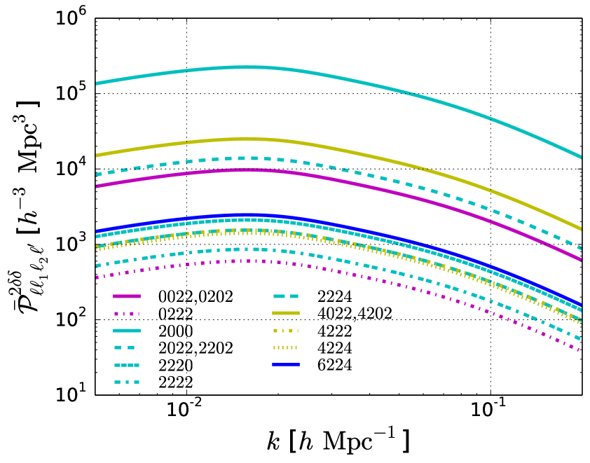
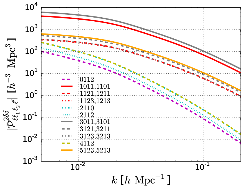
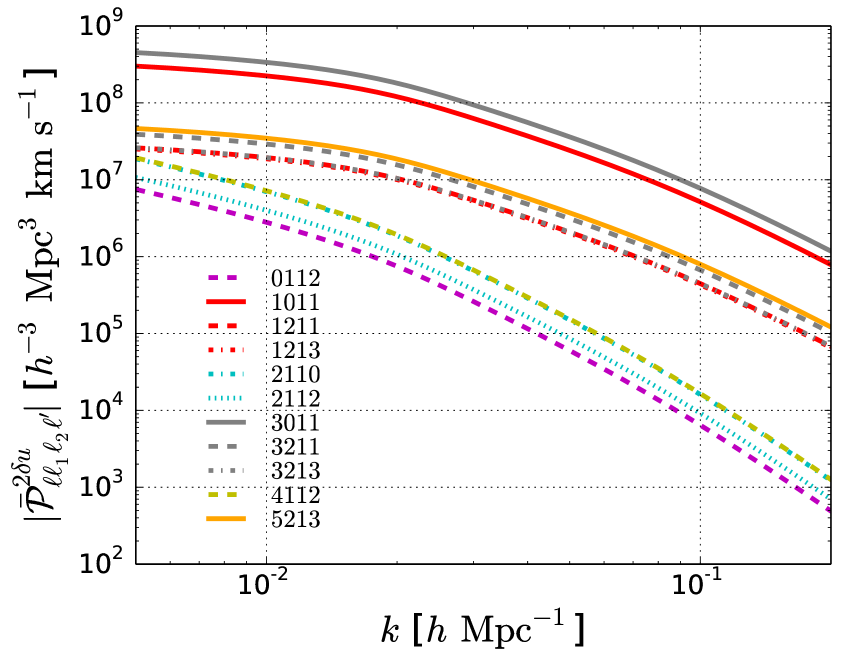
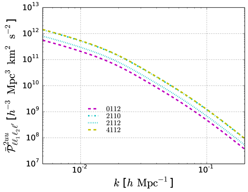
Figure 1: All nonvanishing components of 𝒫¯122δδsuperscriptsubscript¯𝒫subscript1subscript2superscript2𝛿𝛿\bar{\cal P}_{\ell\ell_{1}\ell_{2}\ell^{\prime}}^{2\delta\delta} (top two panels), 𝒫¯122δusuperscriptsubscript¯𝒫subscript1subscript2superscript2𝛿𝑢\bar{\cal P}_{\ell\ell_{1}\ell_{2}\ell^{\prime}}^{2\delta u} (bottom left panel) and 𝒫¯122uusuperscriptsubscript¯𝒫subscript1subscript2superscript2𝑢𝑢\bar{\cal P}_{\ell\ell_{1}\ell_{2}\ell^{\prime}}^{2uu} (bottom right panel), obtained from eq. (3.12), as a function of k𝑘k at b=2.0𝑏2.0b=2.0, z=0.5𝑧0.5z=0.5 and α=2𝛼2\alpha=2. The label of each curve represents the value of 12subscript1subscript2superscript\ell\ell_{1}\ell_{2}\ell^{\prime}. These signals are generated in, e.g., an inflationary model where a spin-1 vector couples to a scalar.

It is confirmed from this that nonzero L>0𝐿0L>0 coefficients are the distinctive features of the isotropy-breaking signal. The selection rules of h12subscriptsubscript1subscript2superscripth_{\ell_{1}\ell_{2}\ell^{\prime}} and hLsubscriptsuperscript𝐿h_{\ell\ell^{\prime}L} restrict the allowed multipole domain to |12|1+2subscript1subscript2superscriptsubscript1subscript2|\ell_{1}-\ell_{2}|\leq\ell^{\prime}\leq\ell_{1}+\ell_{2}, ||L+superscript𝐿superscript|\ell-\ell^{\prime}|\leq L\leq\ell+\ell^{\prime}, 1+2+=evensubscript1subscript2superscripteven\ell_{1}+\ell_{2}+\ell^{\prime}=\rm even and ++L=evensuperscript𝐿even\ell+\ell^{\prime}+L=\rm even. The total number of nonvanishing TripoSH coefficients therefore increases with L𝐿L. For example, 32 𝒫¯122δδsuperscriptsubscript¯𝒫subscript1subscript2superscript2𝛿𝛿\bar{\cal P}_{\ell\ell_{1}\ell_{2}\ell^{\prime}}^{2\delta\delta}, 11 𝒫¯122δusuperscriptsubscript¯𝒫subscript1subscript2superscript2𝛿𝑢\bar{\cal P}_{\ell\ell_{1}\ell_{2}\ell^{\prime}}^{2\delta u} and 4 𝒫¯122uusuperscriptsubscript¯𝒫subscript1subscript2superscript2𝑢𝑢\bar{\cal P}_{\ell\ell_{1}\ell_{2}\ell^{\prime}}^{2uu}, and 36 𝒫¯124δδsuperscriptsubscript¯𝒫subscript1subscript2superscript4𝛿𝛿\bar{\cal P}_{\ell\ell_{1}\ell_{2}\ell^{\prime}}^{4\delta\delta}, 12 𝒫¯124δusuperscriptsubscript¯𝒫subscript1subscript2superscript4𝛿𝑢\bar{\cal P}_{\ell\ell_{1}\ell_{2}\ell^{\prime}}^{4\delta u} and 4 𝒫¯124uusuperscriptsubscript¯𝒫subscript1subscript2superscript4𝑢𝑢\bar{\cal P}_{\ell\ell_{1}\ell_{2}\ell^{\prime}}^{4uu} do not vanish for L=2𝐿2L=2 and 444, respectively.

One can see the shapes of 𝒫¯122δδsuperscriptsubscript¯𝒫subscript1subscript2superscript2𝛿𝛿\bar{\cal P}_{\ell\ell_{1}\ell_{2}\ell^{\prime}}^{2\delta\delta}, 𝒫¯122δusuperscriptsubscript¯𝒫subscript1subscript2superscript2𝛿𝑢\bar{\cal P}_{\ell\ell_{1}\ell_{2}\ell^{\prime}}^{2\delta u} and 𝒫¯122uusuperscriptsubscript¯𝒫subscript1subscript2superscript2𝑢𝑢\bar{\cal P}_{\ell\ell_{1}\ell_{2}\ell^{\prime}}^{2uu} in figure 1. The coefficients sourced by the monopole c0δsuperscriptsubscript𝑐0𝛿c_{0}^{\delta}, corresponding to 1=0subscript10\ell_{1}=0 and/or 2=0subscript20\ell_{2}=0, have the significant amplitudes. The coefficients for 1=1subscript11\ell_{1}=1 and/or 2=1subscript21\ell_{2}=1 have relatively red-tilted shapes because c1X(k)k1proportional-tosuperscriptsubscript𝑐1𝑋𝑘superscript𝑘1c_{1}^{X}(k)\propto k^{-1}.

3.3 Covariance

Here, we compute the covariance of the TripoSH coefficient. The 2PCF reconstructed from a single realization is given by

ξ^X1X2(𝐬12,s^1,s^2)=d3k(2π)3ei𝐤𝐬12P^X1X2(𝐤,s^1,s^2),superscript^𝜉subscript𝑋1subscript𝑋2subscript𝐬12subscript^𝑠1subscript^𝑠2superscript𝑑3𝑘superscript2𝜋3superscript𝑒𝑖𝐤subscript𝐬12superscript^𝑃subscript𝑋1subscript𝑋2𝐤subscript^𝑠1subscript^𝑠2\hat{\xi}^{X_{1}X_{2}}({\bf s}_{12},\hat{s}_{1},\hat{s}_{2})=\int\frac{d^{3}k}{(2\pi)^{3}}e^{i{\bf k}\cdot{\bf s}_{12}}\hat{P}^{X_{1}X_{2}}({\bf k},\hat{s}_{1},\hat{s}_{2}), (3.13)

where

P^X1X2(𝐤,s^1,s^2)1VFX1(𝐤,s^1)FX2(𝐤,s^2)PnoiseX1X2.superscript^𝑃subscript𝑋1subscript𝑋2𝐤subscript^𝑠1subscript^𝑠21𝑉superscript𝐹subscript𝑋1𝐤subscript^𝑠1superscript𝐹subscript𝑋2𝐤subscript^𝑠2superscriptsubscript𝑃noisesubscript𝑋1subscript𝑋2\hat{P}^{X_{1}X_{2}}({\bf k},\hat{s}_{1},\hat{s}_{2})\equiv\frac{1}{V}F^{X_{1}}({\bf k},\hat{s}_{1})F^{X_{2}}(-{\bf k},\hat{s}_{2})-P_{\rm noise}^{X_{1}X_{2}}. (3.14)

with V𝑉V the survey volume and PnoiseX1X2superscriptsubscript𝑃noisesubscript𝑋1subscript𝑋2P_{\rm noise}^{X_{1}X_{2}} the power spectrum of the shot noise. We regard ξX1X2superscript𝜉subscript𝑋1subscript𝑋2\xi^{X_{1}X_{2}}, PX1X2superscript𝑃subscript𝑋1subscript𝑋2P^{X_{1}X_{2}} and their decomposition coefficients with hats as quantities estimated from a single realization henceforth.

We assume Gaussianity of FXsuperscript𝐹𝑋F^{X}; thus, the covariance of P^X1X2superscript^𝑃subscript𝑋1subscript𝑋2\hat{P}^{X_{1}X_{2}} can be simplified to

P^X1X2(𝐤,s^1,s^2)P^X~1X~2(𝐤~,s~^1,s~^2)csubscriptexpectationsuperscript^𝑃subscript𝑋1subscript𝑋2𝐤subscript^𝑠1subscript^𝑠2superscript^𝑃subscript~𝑋1subscript~𝑋2~𝐤subscript^~𝑠1subscript^~𝑠2𝑐\displaystyle\Braket{\hat{P}^{X_{1}X_{2}}({\bf k},\hat{s}_{1},\hat{s}_{2})\hat{P}^{\tilde{X}_{1}\tilde{X}_{2}}(\tilde{\bf k},\hat{\tilde{s}}_{1},\hat{\tilde{s}}_{2})}_{c}
=4πδk,k~Nk[δ(2)(k^+k~^)PtotX1X~1(𝐤,s^1,s~^1)PtotX2X~2(𝐤,s^2,s~^2)\displaystyle\qquad=4\pi\frac{\delta_{k,\tilde{k}}}{N_{k}}\left[\delta^{(2)}(\hat{k}+\hat{\tilde{k}})P_{\rm tot}^{X_{1}\tilde{X}_{1}}({\bf k},\hat{s}_{1},\hat{\tilde{s}}_{1})P_{\rm tot}^{X_{2}\tilde{X}_{2}}(-{\bf k},\hat{s}_{2},\hat{\tilde{s}}_{2})\right.
+δ(2)(k^k~^)PtotX1X~2(𝐤,s^1,s~^2)PtotX2X~1(𝐤,s^2,s~^1)],\displaystyle\qquad\qquad\qquad\left.+\delta^{(2)}(\hat{k}-\hat{\tilde{k}})P_{\rm tot}^{X_{1}\tilde{X}_{2}}({\bf k},\hat{s}_{1},\hat{\tilde{s}}_{2})P_{\rm tot}^{X_{2}\tilde{X}_{1}}(-{\bf k},\hat{s}_{2},\hat{\tilde{s}}_{1})\right], (3.15)

where Nk=Vk2dk/(2π2)subscript𝑁𝑘𝑉superscript𝑘2𝑑𝑘2superscript𝜋2N_{k}=Vk^{2}dk/(2\pi^{2}) and PtotX1X2PX1X2+PnoiseX1X2superscriptsubscript𝑃totsubscript𝑋1subscript𝑋2superscript𝑃subscript𝑋1subscript𝑋2superscriptsubscript𝑃noisesubscript𝑋1subscript𝑋2P_{\rm tot}^{X_{1}X_{2}}\equiv P^{X_{1}X_{2}}+P_{\rm noise}^{X_{1}X_{2}}. Besides, supposing that the anisotropic contributions in PX1X2superscript𝑃subscript𝑋1subscript𝑋2P^{X_{1}X_{2}} are negligibly small; namely |GL1,M|G00much-less-thansubscript𝐺𝐿1𝑀subscript𝐺00|G_{L\geq 1,M}|\ll G_{00}, PtotX1X2superscriptsubscript𝑃totsubscript𝑋1subscript𝑋2P_{\rm tot}^{X_{1}X_{2}} is expressed as

PtotX1X2(𝐤,s^1,s^2)=j1j2(1)j2pj1j2X1X2(k)j1(k^s^1)j2(k^s^2),superscriptsubscript𝑃totsubscript𝑋1subscript𝑋2𝐤subscript^𝑠1subscript^𝑠2subscriptsubscript𝑗1subscript𝑗2superscript1subscript𝑗2superscriptsubscript𝑝subscript𝑗1subscript𝑗2subscript𝑋1subscript𝑋2𝑘subscriptsubscript𝑗1^𝑘subscript^𝑠1subscriptsubscript𝑗2^𝑘subscript^𝑠2P_{\rm tot}^{X_{1}X_{2}}({\bf k},\hat{s}_{1},\hat{s}_{2})=\sum_{j_{1}j_{2}}(-1)^{j_{2}}p_{j_{1}j_{2}}^{X_{1}X_{2}}(k){\cal L}_{j_{1}}(\hat{k}\cdot\hat{s}_{1}){\cal L}_{j_{2}}(\hat{k}\cdot\hat{s}_{2}), (3.16)

where

pj1j2X1X2(k)cj1X1(k)cj2X2(k)P¯m(k)+PnoiseX1X2δj1,0δj2,0.superscriptsubscript𝑝subscript𝑗1subscript𝑗2subscript𝑋1subscript𝑋2𝑘superscriptsubscript𝑐subscript𝑗1subscript𝑋1𝑘superscriptsubscript𝑐subscript𝑗2subscript𝑋2𝑘subscript¯𝑃𝑚𝑘superscriptsubscript𝑃noisesubscript𝑋1subscript𝑋2subscript𝛿subscript𝑗10subscript𝛿subscript𝑗20p_{j_{1}j_{2}}^{X_{1}X_{2}}(k)\equiv c_{j_{1}}^{X_{1}}(k)c_{j_{2}}^{X_{2}}(k)\bar{P}_{m}(k)+P_{\rm noise}^{X_{1}X_{2}}\delta_{j_{1},0}\delta_{j_{2},0}. (3.17)

The covariance of Π^12LMX1X2superscriptsubscript^Πsubscript1subscript2superscript𝐿𝑀subscript𝑋1subscript𝑋2\hat{\Pi}_{\ell\ell_{1}\ell_{2}\ell^{\prime}}^{LMX_{1}X_{2}} is obtained through the double TripoSH decomposition of the covariance of P^X1X2superscript^𝑃subscript𝑋1subscript𝑋2\hat{P}^{X_{1}X_{2}} as

Π^12LMX1X2(k)Π^~~1~2~L~M~X~1X~2(k~)c=d2k^d2s^1d2s^2d2k~^d2s~^1d2s~^2subscriptexpectationsuperscriptsubscript^Πsubscript1subscript2superscript𝐿𝑀subscript𝑋1subscript𝑋2𝑘superscriptsubscript^Π~subscript~1subscript~2superscript~~𝐿~𝑀subscript~𝑋1subscript~𝑋2~𝑘𝑐superscript𝑑2^𝑘superscript𝑑2subscript^𝑠1superscript𝑑2subscript^𝑠2superscript𝑑2^~𝑘superscript𝑑2subscript^~𝑠1superscript𝑑2subscript^~𝑠2\displaystyle\Braket{\hat{\Pi}_{\ell\ell_{1}\ell_{2}\ell^{\prime}}^{LMX_{1}X_{2}}(k)\hat{\Pi}_{\tilde{\ell}\tilde{\ell}_{1}\tilde{\ell}_{2}\tilde{\ell}^{\prime}}^{\tilde{L}\tilde{M}\tilde{X}_{1}\tilde{X}_{2}}(\tilde{k})}_{c}=\int d^{2}\hat{k}\int d^{2}\hat{s}_{1}\int d^{2}\hat{s}_{2}\,\int d^{2}\hat{\tilde{k}}\int d^{2}\hat{\tilde{s}}_{1}\int d^{2}\hat{\tilde{s}}_{2}
×𝒳12LM(k^,s^1,s^2)𝒳~~1~2~L~M~(k~^,s~^1,s~^2)P^X1X2(𝐤,s^1,s^2)P^X~1X~2(𝐤~,s~^1,s~^2)c.absentsuperscriptsubscript𝒳subscript1subscript2superscript𝐿𝑀^𝑘subscript^𝑠1subscript^𝑠2superscriptsubscript𝒳~subscript~1subscript~2superscript~~𝐿~𝑀^~𝑘subscript^~𝑠1subscript^~𝑠2subscriptexpectationsuperscript^𝑃subscript𝑋1subscript𝑋2𝐤subscript^𝑠1subscript^𝑠2superscript^𝑃subscript~𝑋1subscript~𝑋2~𝐤subscript^~𝑠1subscript^~𝑠2𝑐\displaystyle\qquad\times{\cal X}_{\ell\ell_{1}\ell_{2}\ell^{\prime}}^{LM*}(\hat{k},\hat{s}_{1},\hat{s}_{2}){\cal X}_{\tilde{\ell}\tilde{\ell}_{1}\tilde{\ell}_{2}\tilde{\ell}^{\prime}}^{\tilde{L}\tilde{M}*}(\hat{\tilde{k}},\hat{\tilde{s}}_{1},\hat{\tilde{s}}_{2})\Braket{\hat{P}^{X_{1}X_{2}}({\bf k},\hat{s}_{1},\hat{s}_{2})\hat{P}^{\tilde{X}_{1}\tilde{X}_{2}}(\tilde{\bf k},\hat{\tilde{s}}_{1},\hat{\tilde{s}}_{2})}_{c}. (3.18)

In a similar way to the derivation of eq. (3.10), we can simplify the s^1subscript^𝑠1\hat{s}_{1}, s^2subscript^𝑠2\hat{s}_{2}, s~^1subscript^~𝑠1\hat{\tilde{s}}_{1} and s~^2subscript^~𝑠2\hat{\tilde{s}}_{2} integrals by means of eq. (B.4). Via the transformation into the reduced coefficient by eq. (3.6), we derive the form of the covariance matrix of 𝒫^12LMX1X2superscriptsubscript^𝒫subscript1subscript2superscript𝐿𝑀subscript𝑋1subscript𝑋2\hat{\cal P}_{\ell\ell_{1}\ell_{2}\ell^{\prime}}^{LMX_{1}X_{2}}, reading

𝐂𝒫;𝒫subscript𝐂𝒫superscript𝒫\displaystyle{\bf C}_{{\cal P};{\cal P}^{*}} \displaystyle\equiv 𝒫^12LMX1X2(k)𝒫^~~1~2~L~M~X~1X~2(k~)csubscriptexpectationsuperscriptsubscript^𝒫subscript1subscript2superscript𝐿𝑀subscript𝑋1subscript𝑋2𝑘superscriptsubscript^𝒫~subscript~1subscript~2superscript~~𝐿~𝑀subscript~𝑋1subscript~𝑋2~𝑘𝑐\displaystyle\Braket{\hat{\cal P}_{\ell\ell_{1}\ell_{2}\ell^{\prime}}^{LMX_{1}X_{2}}(k)\hat{\cal P}_{\tilde{\ell}\tilde{\ell}_{1}\tilde{\ell}_{2}\tilde{\ell}^{\prime}}^{\tilde{L}\tilde{M}\tilde{X}_{1}\tilde{X}_{2}*}(\tilde{k})}_{c} (3.19)
=\displaystyle= δL,L~δM,M~δk,k~NkΥ12;~~1~2~L;X1X2;X~1X~2(k),subscript𝛿𝐿~𝐿subscript𝛿𝑀~𝑀subscript𝛿𝑘~𝑘subscript𝑁𝑘superscriptsubscriptΥsubscript1subscript2superscript~subscript~1subscript~2superscript~𝐿subscript𝑋1subscript𝑋2subscript~𝑋1subscript~𝑋2𝑘\displaystyle\delta_{L,\tilde{L}}\delta_{M,\tilde{M}}\frac{\delta_{k,\tilde{k}}}{N_{k}}\Upsilon_{\ell\ell_{1}\ell_{2}\ell^{\prime};\tilde{\ell}\tilde{\ell}_{1}\tilde{\ell}_{2}\tilde{\ell}^{\prime}}^{L;X_{1}X_{2};\tilde{X}_{1}\tilde{X}_{2}}(k),

where

Υ12;~~1~2~L;X1X2;X~1X~2(k)superscriptsubscriptΥsubscript1subscript2superscript~subscript~1subscript~2superscript~𝐿subscript𝑋1subscript𝑋2subscript~𝑋1subscript~𝑋2𝑘\displaystyle\Upsilon_{\ell\ell_{1}\ell_{2}\ell^{\prime};\tilde{\ell}\tilde{\ell}_{1}\tilde{\ell}_{2}\tilde{\ell}^{\prime}}^{L;X_{1}X_{2};\tilde{X}_{1}\tilde{X}_{2}}(k) \displaystyle\equiv (4π)4(1)2+~1h122hL2h~1~2~2h~~L2(21+1)(22+1)(2+1)(2~1+1)(2~2+1)(2~+1)(2L+1)superscript4𝜋4superscript1subscript2subscript~1superscriptsubscriptsubscript1subscript2superscript2superscriptsubscriptsuperscript𝐿2superscriptsubscriptsubscript~1subscript~2superscript~2superscriptsubscript~superscript~𝐿22subscript112subscript212superscript12subscript~112subscript~212superscript~12𝐿1\displaystyle\frac{(4\pi)^{4}(-1)^{\ell_{2}+\tilde{\ell}_{1}}h_{\ell_{1}\ell_{2}\ell^{\prime}}^{2}h_{\ell\ell^{\prime}L}^{2}h_{\tilde{\ell}_{1}\tilde{\ell}_{2}\tilde{\ell}^{\prime}}^{2}h_{\tilde{\ell}\tilde{\ell}^{\prime}L}^{2}}{(2\ell_{1}+1)(2\ell_{2}+1)(2\ell^{\prime}+1)(2\tilde{\ell}_{1}+1)(2\tilde{\ell}_{2}+1)(2\tilde{\ell}^{\prime}+1)(2L+1)} (3.20)
×[p1~1X1X~1(k)p2~2X2X~2(k)+(1)Lp1~2X1X~2(k)p2~1X2X~1(k)],absentdelimited-[]superscriptsubscript𝑝subscript1subscript~1subscript𝑋1subscript~𝑋1𝑘superscriptsubscript𝑝subscript2subscript~2subscript𝑋2subscript~𝑋2𝑘superscript1𝐿superscriptsubscript𝑝subscript1subscript~2subscript𝑋1subscript~𝑋2𝑘superscriptsubscript𝑝subscript2subscript~1subscript𝑋2subscript~𝑋1𝑘\displaystyle\times\left[p_{\ell_{1}\tilde{\ell}_{1}}^{X_{1}\tilde{X}_{1}}(k)p_{\ell_{2}\tilde{\ell}_{2}}^{X_{2}\tilde{X}_{2}}(k)+(-1)^{L}p_{\ell_{1}\tilde{\ell}_{2}}^{X_{1}\tilde{X}_{2}}(k)p_{\ell_{2}\tilde{\ell}_{1}}^{X_{2}\tilde{X}_{1}}(k)\right],

with pj1j2X1X2superscriptsubscript𝑝subscript𝑗1subscript𝑗2subscript𝑋1subscript𝑋2p_{j_{1}j_{2}}^{X_{1}X_{2}} the coefficient of the double Legendre expansion of PtotX1X2superscriptsubscript𝑃totsubscript𝑋1subscript𝑋2P_{\rm tot}^{X_{1}X_{2}}, defined in eqs. (3.16) and (3.17). This can be straightforwardly transformed into the covariance of Ξ^12LMX1X2superscriptsubscript^Ξsubscript1subscript2superscript𝐿𝑀subscript𝑋1subscript𝑋2\hat{\Xi}_{\ell\ell_{1}\ell_{2}\ell^{\prime}}^{LMX_{1}X_{2}} by means of eqs. (3.4) and (3.6).

In analogy with the L=0𝐿0L=0 case [41], we also find from eqs. (3.20) and (3.17) that the covariance becomes independent of PnoiseX1X2superscriptsubscript𝑃noisesubscript𝑋1subscript𝑋2P_{\rm noise}^{X_{1}X_{2}} at some special multipole configurations, e.g., where none or only one of 1subscript1\ell_{1}, 2subscript2\ell_{2}, ~1subscript~1\tilde{\ell}_{1} and ~2subscript~2\tilde{\ell}_{2} becomes 00. The covariance then takes the minimized form as

Υ12;~~1~2~L;X1X2;X~1X~2(k)=[1+(1)L]𝒫¯12LX1X2(k)𝒫¯~~1~2~LX~1X~2(k).superscriptsubscriptΥsubscript1subscript2superscript~subscript~1subscript~2superscript~𝐿subscript𝑋1subscript𝑋2subscript~𝑋1subscript~𝑋2𝑘delimited-[]1superscript1𝐿superscriptsubscript¯𝒫subscript1subscript2superscript𝐿subscript𝑋1subscript𝑋2𝑘superscriptsubscript¯𝒫~subscript~1subscript~2superscript~𝐿subscript~𝑋1subscript~𝑋2𝑘\Upsilon_{\ell\ell_{1}\ell_{2}\ell^{\prime};\tilde{\ell}\tilde{\ell}_{1}\tilde{\ell}_{2}\tilde{\ell}^{\prime}}^{L;X_{1}X_{2};\tilde{X}_{1}\tilde{X}_{2}}(k)=\left[1+(-1)^{L}\right]\bar{\cal P}_{\ell\ell_{1}\ell_{2}\ell^{\prime}}^{LX_{1}X_{2}}(k)\bar{\cal P}_{\tilde{\ell}\tilde{\ell}_{1}\tilde{\ell}_{2}\tilde{\ell}^{\prime}}^{L\tilde{X}_{1}\tilde{X}_{2}*}(k). (3.21)

This form reveals that there is no entanglement between different multipole moments, which appear in the PP-limit covariance (A.15) or (A.16). This fact results in the improvement of the detectability of GLMsubscript𝐺𝐿𝑀G_{LM} as shown in the next section.

4 Expected errors on gLMsubscript𝑔𝐿𝑀g_{LM}

In this section, we forecast the detectability of the anisotropic amplitude GL>0,Msubscript𝐺𝐿0𝑀G_{L>0,M} for L=even𝐿evenL={\rm even} by computing the Fisher matrix. We assume that GLMsubscript𝐺𝐿𝑀G_{LM} has a power-law shape,

GLM(k)=gLM(kk)q,subscript𝐺𝐿𝑀𝑘subscript𝑔𝐿𝑀superscript𝑘subscript𝑘𝑞G_{LM}(k)=g_{LM}\left(\frac{k}{k_{*}}\right)^{q}, (4.1)

with k0.05Mpc1subscript𝑘0.05superscriptMpc1k_{*}\equiv 0.05\,{\rm Mpc}^{-1} the pivot scale adopted in the CMB analysis [15, 14, 16]. The power-law shape is naturally predicted, e.g, in vector inflation models [53, 55, 18]. We then compute 1σ1𝜎1\sigma errors on gLMsubscript𝑔𝐿𝑀g_{LM} for five degrees of tilt: q=±2𝑞plus-or-minus2q=\pm 2, ±1plus-or-minus1\pm 1 and 00.

4.1 Fisher matrix formalism

The Fisher matrix for gLMsubscript𝑔𝐿𝑀g_{LM} is defined as

FgLM,gL~M~𝓟gLM𝐂𝒫;𝒫1𝓟𝖳gL~M~,subscript𝐹subscript𝑔𝐿𝑀subscript𝑔~𝐿~𝑀superscript𝓟superscriptsubscript𝑔𝐿𝑀subscriptsuperscript𝐂1superscript𝒫𝒫superscript𝓟𝖳subscript𝑔~𝐿~𝑀F_{g_{LM},g_{\tilde{L}\tilde{M}}}\equiv\frac{\partial\boldsymbol{\cal P}^{*}}{\partial g_{LM}^{*}}\,{\bf C}^{-1}_{{\cal P}^{*};{\cal P}}\,\frac{\partial\boldsymbol{\cal P}^{\mathsf{T}}}{\partial g_{\tilde{L}\tilde{M}}}, (4.2)

where 𝓟𝓟\boldsymbol{\cal P} is a vector composed of the TripoSH coefficients, and 𝓟𝖳superscript𝓟𝖳\boldsymbol{\cal P}^{\mathsf{T}} is its transpose. Since the covariance matrix (3.19) is diagonalized with respect to L𝐿L and M𝑀M, the Fisher matrix is also diagonalized as

FgLM,gL~M~=LδL,L~δM,M~.subscript𝐹subscript𝑔𝐿𝑀subscript𝑔~𝐿~𝑀subscript𝐿subscript𝛿𝐿~𝐿subscript𝛿𝑀~𝑀F_{g_{LM},g_{\tilde{L}\tilde{M}}}={\cal F}_{L}\delta_{L,\tilde{L}}\delta_{M,\tilde{M}}. (4.3)

Taking the continuous limit kΔk𝑑ksubscript𝑘Δ𝑘differential-d𝑘\sum_{k}\Delta k\to\int dk, we obtain

L=X1X2X~1X~2Vkminkmaxk2dk(2π)3(kk)2q12~~1~2~𝒫¯12LX1X2(k)(Υ1)12;~~1~2~L;X1X2;X~1X~2(k)𝒫¯~~1~2~LX~1X~2(k),subscript𝐿subscriptsubscript𝑋1subscript𝑋2subscript~𝑋1subscript~𝑋2𝑉superscriptsubscriptsubscript𝑘minsubscript𝑘maxsuperscript𝑘2𝑑𝑘superscript2𝜋3superscript𝑘subscript𝑘2𝑞subscriptsubscript1subscript2superscript~subscript~1subscript~2superscript~superscriptsubscript¯𝒫subscript1subscript2superscript𝐿subscript𝑋1subscript𝑋2𝑘superscriptsubscriptsuperscriptΥ1subscript1subscript2superscript~subscript~1subscript~2superscript~𝐿subscript𝑋1subscript𝑋2subscript~𝑋1subscript~𝑋2𝑘superscriptsubscript¯𝒫~subscript~1subscript~2superscript~𝐿subscript~𝑋1subscript~𝑋2𝑘{\cal F}_{L}=\sum_{\begin{subarray}{c}X_{1}X_{2}\\ \tilde{X}_{1}\tilde{X}_{2}\end{subarray}}V\int_{k_{\rm min}}^{k_{\rm max}}\frac{k^{2}dk}{(2\pi)^{3}}\left(\frac{k}{k_{*}}\right)^{2q}\sum_{\begin{subarray}{c}\ell\ell_{1}\ell_{2}\ell^{\prime}\\ \tilde{\ell}\tilde{\ell}_{1}\tilde{\ell}_{2}\tilde{\ell}^{\prime}\end{subarray}}\bar{\cal P}_{\ell\ell_{1}\ell_{2}\ell^{\prime}}^{LX_{1}X_{2}*}(k)(\Upsilon^{-1})_{\ell\ell_{1}\ell_{2}\ell^{\prime};\tilde{\ell}\tilde{\ell}_{1}\tilde{\ell}_{2}\tilde{\ell}^{\prime}}^{L;X_{1}X_{2};\tilde{X}_{1}\tilde{X}_{2}}(k)\bar{\cal P}_{\tilde{\ell}\tilde{\ell}_{1}\tilde{\ell}_{2}\tilde{\ell}^{\prime}}^{L\tilde{X}_{1}\tilde{X}_{2}}(k), (4.4)

where X1X2X~1X~2subscriptsubscript𝑋1subscript𝑋2subscript~𝑋1subscript~𝑋2\sum_{\begin{subarray}{c}X_{1}X_{2}\\ \tilde{X}_{1}\tilde{X}_{2}\end{subarray}} and 12~~1~2~subscriptsubscript1subscript2superscript~subscript~1subscript~2superscript~\sum_{\begin{subarray}{c}\ell\ell_{1}\ell_{2}\ell^{\prime}\\ \tilde{\ell}\tilde{\ell}_{1}\tilde{\ell}_{2}\tilde{\ell}^{\prime}\end{subarray}} should be performed in terms of all observable fields and multipoles one wants to take into account, respectively. One can also compute the Fisher matrix based on Ξ12LMX1X2superscriptsubscriptΞsubscript1subscript2superscript𝐿𝑀subscript𝑋1subscript𝑋2\Xi_{\ell\ell_{1}\ell_{2}\ell^{\prime}}^{LMX_{1}X_{2}}, while a similar result should be obtained since it is related to eq. (4.4) via the simple Hankel transformation (3.4). The expected 1σ1𝜎1\sigma error is computed according to ΔgLM=1/LΔsubscript𝑔𝐿𝑀1subscript𝐿\Delta g_{LM}=1/\sqrt{{\cal F}_{L}}. Numerical results are described in the next subsection.

In the simplest case where one uses the information of only one of the three different 2PCFs (X1X2={δδ,δu,uu}subscript𝑋1subscript𝑋2𝛿𝛿𝛿𝑢𝑢𝑢X_{1}X_{2}=\{\delta\delta,\delta u,uu\}) and a single multipole set, the Fisher matrix is given by

L|12X1X2=Vkminkmaxk2dk(2π)3(kk)2q|𝒫¯12LX1X2(k)|2Υ12;12L;X1X2;X1X2(k).evaluated-atsubscript𝐿subscript1subscript2superscriptsubscript𝑋1subscript𝑋2𝑉superscriptsubscriptsubscript𝑘minsubscript𝑘maxsuperscript𝑘2𝑑𝑘superscript2𝜋3superscript𝑘subscript𝑘2𝑞superscriptsuperscriptsubscript¯𝒫subscript1subscript2superscript𝐿subscript𝑋1subscript𝑋2𝑘2superscriptsubscriptΥsubscript1subscript2superscriptsubscript1subscript2superscript𝐿subscript𝑋1subscript𝑋2subscript𝑋1subscript𝑋2𝑘{\cal F}_{L}|_{\ell\ell_{1}\ell_{2}\ell^{\prime}}^{X_{1}X_{2}}=V\int_{k_{\rm min}}^{k_{\rm max}}\frac{k^{2}dk}{(2\pi)^{3}}\left(\frac{k}{k_{*}}\right)^{2q}\frac{|\bar{\cal P}_{\ell\ell_{1}\ell_{2}\ell^{\prime}}^{LX_{1}X_{2}}(k)|^{2}}{\Upsilon_{\ell\ell_{1}\ell_{2}\ell^{\prime};\ell\ell_{1}\ell_{2}\ell^{\prime}}^{L;X_{1}X_{2};X_{1}X_{2}}(k)}. (4.5)

In particular, for 10subscript10\ell_{1}\neq 0 and 20subscript20\ell_{2}\neq 0, the covariance takes the minimized form (3.21). The Fisher matrix is accordingly maximized and can be analytically computed as

L|12X1X2=Vk316π3×{[(kmaxk)2q+3(kmink)2q+3]12q+3:q32ln(kmaxkmin):q=32.evaluated-atsubscript𝐿subscript1subscript2superscriptsubscript𝑋1subscript𝑋2𝑉superscriptsubscript𝑘316superscript𝜋3casesdelimited-[]superscriptsubscript𝑘maxsubscript𝑘2𝑞3superscriptsubscript𝑘minsubscript𝑘2𝑞312𝑞3:absent𝑞32subscript𝑘maxsubscript𝑘min:absent𝑞32{\cal F}_{L}|_{\ell\ell_{1}\ell_{2}\ell^{\prime}}^{X_{1}X_{2}}=\frac{Vk_{*}^{3}}{16\pi^{3}}\times\begin{cases}\left[\left(\frac{k_{\rm max}}{k_{*}}\right)^{2q+3}-\left(\frac{k_{\rm min}}{k_{*}}\right)^{2q+3}\right]\frac{1}{2q+3}&:q\neq-\frac{3}{2}\\ \ln\left(\frac{k_{\rm max}}{k_{\rm min}}\right)&:q=-\frac{3}{2}\end{cases}. (4.6)

For example, for L=2𝐿2L=2, the following 21+9+4219421+9+4 components take this form,

{2|0112δδ,2|0222δδ,2|1121δδ,2|1123δδ,2|1211δδ,2|1213δδ,2|2110δδ,2|2112δδ,2|2220δδ,2|2222δδ,2|2224δδ,2|3121δδ,2|3123δδ,2|3211δδ,2|3213δδ,2|4112δδ,2|4222δδ,2|4224δδ,2|5123δδ,2|5213δδ,2|6224δδ,{2|0112δu,2|1211δu,2|1213δu,2|2110δu,2|2112δu,2|3211δu,2|3213δu,2|4112δu,2|5213δu,{2|0112uu,2|2110uu,2|2112uu,2|4112uu.casesevaluated-atsubscript20112𝛿𝛿evaluated-atsubscript20222𝛿𝛿otherwiseevaluated-atsubscript21121𝛿𝛿evaluated-atsubscript21123𝛿𝛿evaluated-atsubscript21211𝛿𝛿evaluated-atsubscript21213𝛿𝛿otherwiseevaluated-atsubscript22110𝛿𝛿evaluated-atsubscript22112𝛿𝛿evaluated-atsubscript22220𝛿𝛿evaluated-atsubscript22222𝛿𝛿evaluated-atsubscript22224𝛿𝛿otherwiseevaluated-atsubscript23121𝛿𝛿evaluated-atsubscript23123𝛿𝛿evaluated-atsubscript23211𝛿𝛿evaluated-atsubscript23213𝛿𝛿otherwiseevaluated-atsubscript24112𝛿𝛿evaluated-atsubscript24222𝛿𝛿evaluated-atsubscript24224𝛿𝛿otherwiseevaluated-atsubscript25123𝛿𝛿evaluated-atsubscript25213𝛿𝛿otherwiseevaluated-atsubscript26224𝛿𝛿otherwisecasesevaluated-atsubscript20112𝛿𝑢otherwiseevaluated-atsubscript21211𝛿𝑢evaluated-atsubscript21213𝛿𝑢otherwiseevaluated-atsubscript22110𝛿𝑢evaluated-atsubscript22112𝛿𝑢otherwiseevaluated-atsubscript23211𝛿𝑢evaluated-atsubscript23213𝛿𝑢otherwiseevaluated-atsubscript24112𝛿𝑢otherwiseevaluated-atsubscript25213𝛿𝑢otherwisecasesevaluated-atsubscript20112𝑢𝑢otherwiseevaluated-atsubscript22110𝑢𝑢evaluated-atsubscript22112𝑢𝑢otherwiseevaluated-atsubscript24112𝑢𝑢otherwise\displaystyle\begin{split}&\begin{cases}{\cal F}_{2}|_{0112}^{\delta\delta},\ \ {\cal F}_{2}|_{0222}^{\delta\delta},\\ {\cal F}_{2}|_{1121}^{\delta\delta},\ \ {\cal F}_{2}|_{1123}^{\delta\delta},\ \ {\cal F}_{2}|_{1211}^{\delta\delta},\ \ {\cal F}_{2}|_{1213}^{\delta\delta},\\ {\cal F}_{2}|_{2110}^{\delta\delta},\ \ {\cal F}_{2}|_{2112}^{\delta\delta},\ \ {\cal F}_{2}|_{2220}^{\delta\delta},\ \ {\cal F}_{2}|_{2222}^{\delta\delta},\ \ {\cal F}_{2}|_{2224}^{\delta\delta},\\ {\cal F}_{2}|_{3121}^{\delta\delta},\ \ {\cal F}_{2}|_{3123}^{\delta\delta},\ \ {\cal F}_{2}|_{3211}^{\delta\delta},\ \ {\cal F}_{2}|_{3213}^{\delta\delta},\\ {\cal F}_{2}|_{4112}^{\delta\delta},\ \ {\cal F}_{2}|_{4222}^{\delta\delta},\ \ {\cal F}_{2}|_{4224}^{\delta\delta},\\ {\cal F}_{2}|_{5123}^{\delta\delta},\ \ {\cal F}_{2}|_{5213}^{\delta\delta},\\ {\cal F}_{2}|_{6224}^{\delta\delta},\end{cases}\\ &\begin{cases}{\cal F}_{2}|_{0112}^{\delta u},\\ {\cal F}_{2}|_{1211}^{\delta u},\ \ {\cal F}_{2}|_{1213}^{\delta u},\\ {\cal F}_{2}|_{2110}^{\delta u},\ \ {\cal F}_{2}|_{2112}^{\delta u},\\ {\cal F}_{2}|_{3211}^{\delta u},\ \ {\cal F}_{2}|_{3213}^{\delta u},\\ {\cal F}_{2}|_{4112}^{\delta u},\\ {\cal F}_{2}|_{5213}^{\delta u},\end{cases}\qquad\begin{cases}{\cal F}_{2}|_{0112}^{uu},\\ {\cal F}_{2}|_{2110}^{uu},\ \ {\cal F}_{2}|_{2112}^{uu},\\ {\cal F}_{2}|_{4112}^{uu}.\end{cases}\end{split} (4.7)

We stress that eq. (4.6) exactly holds irrespective of the shot noise level. In contrast, in the PP-limit analysis [21, 19], eq. (4.6) has been approximately derived for X1X2=δδsubscript𝑋1subscript𝑋2𝛿𝛿X_{1}X_{2}=\delta\delta, though we then must assume a noiseless survey (see the next subsection and appendix A.4 for details).

4.2 Results
Refer to caption
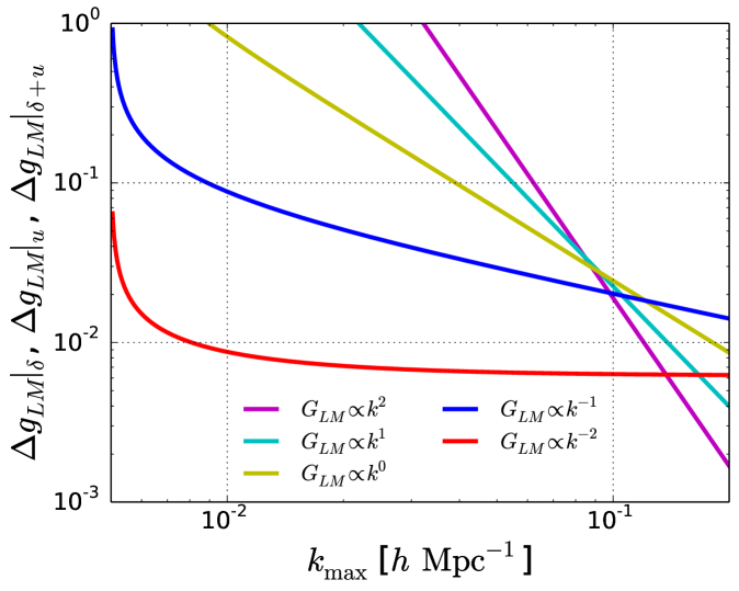
Figure 2: Expected 1σ1𝜎1\sigma errors on gLMsubscript𝑔𝐿𝑀g_{LM} from the δ𝛿\delta-only, u𝑢u-only and δ+u𝛿𝑢\delta+u data as a function of kmaxsubscript𝑘maxk_{\rm max} when GLMk±2proportional-tosubscript𝐺𝐿𝑀superscript𝑘plus-or-minus2G_{LM}\propto k^{\pm 2}, k±1superscript𝑘plus-or-minus1k^{\pm 1} and k0superscript𝑘0k^{0}. These completely overlap with each other. We here adopt kmin=0.005hMpc1subscript𝑘min0.005superscriptMpc1k_{\rm min}=0.005h\,\rm Mpc^{-1} and V=2.5h3Gpc3𝑉2.5superscript3superscriptGpc3V=2.5h^{-3}\,\rm Gpc^{3}.
Refer to caption Refer to caption
Refer to caption
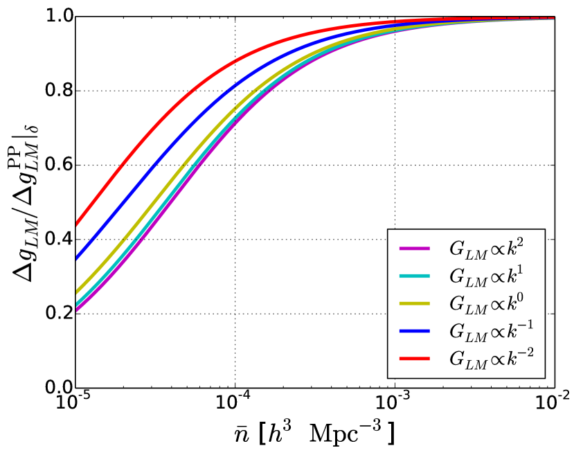
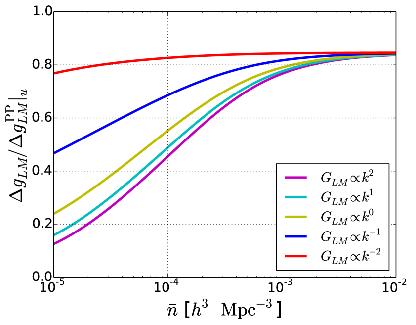
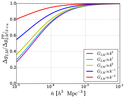
Figure 3: Ratios of expected 1σ1𝜎1\sigma errors on gLMsubscript𝑔𝐿𝑀g_{LM} from the δ𝛿\delta-only, u𝑢u-only and δ+u𝛿𝑢\delta+u data to the counterparts estimated in the PP limit as a function of the number density of observed galaxies n¯¯𝑛\bar{n} when GLMk±2proportional-tosubscript𝐺𝐿𝑀superscript𝑘plus-or-minus2G_{LM}\propto k^{\pm 2}, k±1superscript𝑘plus-or-minus1k^{\pm 1} and k0superscript𝑘0k^{0}. To make this figure, kmin=0.005hMpc1subscript𝑘min0.005superscriptMpc1k_{\rm min}=0.005h\,\rm Mpc^{-1}, kmax=0.1hMpc1subscript𝑘max0.1superscriptMpc1k_{\rm max}=0.1h\,\rm Mpc^{-1}, b=2.0𝑏2.0b=2.0 and z=0.5𝑧0.5z=0.5 are adopted. The results are not so sensitive to the change of these parameters.

Here we discuss numerical results estimated from δ𝛿\delta only (ΔgLM|δevaluated-atΔsubscript𝑔𝐿𝑀𝛿\Delta g_{LM}|_{\delta}), u𝑢u only (ΔgLM|uevaluated-atΔsubscript𝑔𝐿𝑀𝑢\Delta g_{LM}|_{u}) and δ𝛿\delta and u𝑢u jointly (ΔgLM|δ+uevaluated-atΔsubscript𝑔𝐿𝑀𝛿𝑢\Delta g_{LM}|_{\delta+u}). We then find that ΔgLM|δevaluated-atΔsubscript𝑔𝐿𝑀𝛿\Delta g_{LM}|_{\delta}, ΔgLM|uevaluated-atΔsubscript𝑔𝐿𝑀𝑢\Delta g_{LM}|_{u} and ΔgLM|δ+uevaluated-atΔsubscript𝑔𝐿𝑀𝛿𝑢\Delta g_{LM}|_{\delta+u} have identical values, and it coincides with the inverse of the root of eq. (4.6). This means that the corresponding Fisher matrices contain the information of eq. (4.6) in submatrices, while eq. (4.6) already takes the maximized form; thus, there is no additional gain by integrating all multipoles. We also confirm that ΔgLM|δevaluated-atΔsubscript𝑔𝐿𝑀𝛿\Delta g_{LM}|_{\delta}, ΔgLM|uevaluated-atΔsubscript𝑔𝐿𝑀𝑢\Delta g_{LM}|_{u} and ΔgLM|δ+uevaluated-atΔsubscript𝑔𝐿𝑀𝛿𝑢\Delta g_{LM}|_{\delta+u} are robust against the change of L𝐿L, M𝑀M, PnoiseX1X2superscriptsubscript𝑃noisesubscript𝑋1subscript𝑋2P_{\rm noise}^{X_{1}X_{2}}, z𝑧z, b𝑏b, f𝑓f or any cosmological parameter as inferred from eq. (4.6).

Figure 2 describes ΔgLM|δevaluated-atΔsubscript𝑔𝐿𝑀𝛿\Delta g_{LM}|_{\delta}, ΔgLM|uevaluated-atΔsubscript𝑔𝐿𝑀𝑢\Delta g_{LM}|_{u} and ΔgLM|δ+uevaluated-atΔsubscript𝑔𝐿𝑀𝛿𝑢\Delta g_{LM}|_{\delta+u} as a function of kmaxsubscript𝑘maxk_{\rm max} at the level of current experiments: kmin=0.005hMpc1subscript𝑘min0.005superscriptMpc1k_{\rm min}=0.005h\,\rm Mpc^{-1} and V=2.5h3Gpc3𝑉2.5superscript3superscriptGpc3V=2.5h^{-3}\,\rm Gpc^{3}. The kmaxsubscript𝑘maxk_{\rm max} dependence corresponding to the tilt of GLMsubscript𝐺𝐿𝑀G_{LM} is confirmed. The detectability can approach the CMB level ΔgLM102similar-toΔsubscript𝑔𝐿𝑀superscript102\Delta g_{LM}\sim 10^{-2} [19] as kmaxsubscript𝑘maxk_{\rm max} is close to 0.1hMpc10.1superscriptMpc10.1h\,\rm Mpc^{-1}. Surpassing this value is expected in a forthcoming survey by increasing V𝑉V.

Next, we discuss the detectability improvement relative to the PP-limit results ΔgLMPPΔsuperscriptsubscript𝑔𝐿𝑀PP\Delta g_{LM}^{\rm PP} computed from eq. (A.17). In figure 3 we show ΔgLM/ΔgLMPPΔsubscript𝑔𝐿𝑀Δsuperscriptsubscript𝑔𝐿𝑀PP\Delta g_{LM}/\Delta g_{LM}^{\rm PP} as a function of n¯¯𝑛\bar{n}, which determines the sizes of the shot noise spectra according to Pnoiseδδ=1/n¯superscriptsubscript𝑃noise𝛿𝛿1¯𝑛P_{\rm noise}^{\delta\delta}=1/\bar{n}, Pnoiseuu=σu2/n¯superscriptsubscript𝑃noise𝑢𝑢superscriptsubscript𝜎𝑢2¯𝑛P_{\rm noise}^{uu}=\sigma_{u}^{2}/\bar{n} and Pnoiseδu=Pnoiseuδ=0superscriptsubscript𝑃noise𝛿𝑢superscriptsubscript𝑃noise𝑢𝛿0P_{\rm noise}^{\delta u}=P_{\rm noise}^{u\delta}=0, where σu=300km/ssubscript𝜎𝑢300kms\sigma_{u}=300\,\rm km/s is assumed. Note that this ratio is independent of V𝑉V.

The observed fact that ΔgLM/ΔgLMPP1Δsubscript𝑔𝐿𝑀Δsuperscriptsubscript𝑔𝐿𝑀PP1\Delta g_{LM}/\Delta g_{LM}^{\rm PP}\leq 1 for any n¯¯𝑛\bar{n} means that, in detectability, our TripoSH-based analysis always surpasses the PP-limit one. The PP approximation causes nontrivial mode mixings at the covariance level and the degradation of detectability (see appendix A.3 for details). However, the superiority of the TripoSH-based analysis fades in the high number density limit. This is because ΔgLMΔsubscript𝑔𝐿𝑀\Delta g_{LM} remains constant, while ΔgLMPPΔsuperscriptsubscript𝑔𝐿𝑀PP\Delta g_{LM}^{\rm PP} shrinks owing to the reduction of the covariance (A.15). In the noiseless limit (or equivalently, in the large n¯¯𝑛\bar{n} regime), ΔgLM/ΔgLMPP|δevaluated-atΔsubscript𝑔𝐿𝑀Δsuperscriptsubscript𝑔𝐿𝑀PP𝛿\Delta g_{LM}/\Delta g_{LM}^{\rm PP}|_{\delta} reaches 1similar-toabsent1\sim 1, while, interestingly, ΔgLM/ΔgLMPP|uevaluated-atΔsubscript𝑔𝐿𝑀Δsuperscriptsubscript𝑔𝐿𝑀PP𝑢\Delta g_{LM}/\Delta g_{LM}^{\rm PP}|_{u} still remains 0.8similar-toabsent0.8\sim 0.8, meaning that at least 20%similar-toabsentpercent20\sim 20\% improvement is always expected compared to the PP-limit analysis regardless of the shape of GLMsubscript𝐺𝐿𝑀G_{LM}. This benefits from a fact that ΔgLMPP|uevaluated-atΔsuperscriptsubscript𝑔𝐿𝑀PP𝑢\Delta g_{LM}^{\rm PP}|_{u} is not minimized even in the noiseless limit due to residual mode mixings in the PP-limit covariance (see appendix A.4 for a detailed explanation). Comparing eq. (4.6) with the PP-limit analytic results (A.20) and (A.22), these values are recovered.

On the other hand, the superiority of the TripoSH-based analysis becomes remarkable as GLM(k)subscript𝐺𝐿𝑀𝑘G_{LM}(k) is blue-tilted. In the blue-tilted case the bias due to the shot noise is more effective at larger k𝑘k and hence ΔgLMPPΔsuperscriptsubscript𝑔𝐿𝑀PP\Delta g_{LM}^{\rm PP} is further smoothed. In contrast, ΔgLMΔsubscript𝑔𝐿𝑀\Delta g_{LM} is free from this effect (because of no dependence on n¯¯𝑛\bar{n}) and therefore the gap between them is widened.

5 Conclusions

In this paper, we, for the first time, have examined the detectability of cosmic statistical anisotropy via galaxy density and velocity surveys without assuming the PP approximation. To extract the anisotropic signal from the 2PCF of the density and velocity fields, we have performed a TripoSH decomposition. The covariance of the TripoSH coefficient has been computed for the first time, and from the resultant analytic expression, the absence of nontrivial mixings between each multipole moment, which appear in the PP-limit covariance, has been confirmed. Owing to this fact, the covariance is minimized, resulting in the optimization of signal detectability. Via a Fisher matrix calculation, we have shown that, in terms of the detectability of statistical anisotropy, our TripoSH-based estimation always has an advantage over the previous PP-limit one. Remarkable superiority has been confirmed, especially in the cases that the shot noise level is large and that target statistical anisotropy has a blue-tilted shape in Fourier space.

In upcoming all-sky surveys [23, 24, 25], wide-angle effects in the 2PCF, which cannot be treated by the PP-limit formalism, will play a critical role. As we have shown in this paper, inclusion of wide-angle effects in the data analysis is beneficial for the cosmic isotropy test. Since the TripoSH decomposition is applicable as long as two LOS directions are distinguishable from each other, an analysis of no all-sky survey data could even achieve a similar detectability improvement. As some experiments will start running in the few years [23, 60], a feasible estimator of the TripoSH coefficient and a methodology for removing artificial anisotropic contaminations due to, e.g., asymmetric survey geometry should be immediately established.

Throughout this paper, linear theory has always been adopted, and any general relativistic effect (e.g. [33]) has not been taken into account. Hence, the reasonability of our estimates is not trivial for extremely large or small scales. The geometrical distortion produced by the Alcock-Paczynski effect [61, 62, 63], has also not been included in our analysis since the geometrical distortion on the curved sky is not trivial. These should be clarified in future works.

Acknowledgments

M. S. is supported by JSPS KAKENHI Grant Nos. JP19K14718 and JP20H05859. T. O. acknowledges support from the Ministry of Science and Technology of Taiwan under Grant Nos. MOST 106-2119-M-001-031-MY3 and MOST 109-2112-M-001-027- and the Career Development Award, Academia Sinica (AS-CDA-108-M02) for the period of 2019 to 2023. K. A. is supported by Grand-in-Aid for JSPS fellows No. JP19J12254. M. S. and K. A. also acknowledge the Center for Computational Astrophysics, National Astronomical Observatory of Japan, for providing the computing resources of the Cray XC50.

Appendix A Expected errors on gLMsubscript𝑔𝐿𝑀g_{LM} in the plane-parallel limit

In this appendix, we discuss the Fisher matrix forecasts for gLMsubscript𝑔𝐿𝑀g_{LM} in the PP limit (s^1=s^2subscript^𝑠1subscript^𝑠2\hat{s}_{1}=\hat{s}_{2}). As for the δ𝛿\delta-only case, there already exist complete discussions in the literature [21, 19, 13], while here it is extended by adding the velocity field.

A.1 Bipolar spherical harmonic decomposition

In the PP limit, the 2PCF is characterized by two angles: s^12subscript^𝑠12\hat{s}_{12} and s^s^1=s^2^𝑠subscript^𝑠1subscript^𝑠2\hat{s}\equiv\hat{s}_{1}=\hat{s}_{2}. In this case, the angular dependence is completely decomposed according to

ξX1X2(𝐬12,s^,s^)=LMξLMX1X2(s12)XLM(s^12,s^),superscript𝜉subscript𝑋1subscript𝑋2subscript𝐬12^𝑠^𝑠subscriptsuperscript𝐿𝑀superscriptsubscript𝜉superscript𝐿𝑀subscript𝑋1subscript𝑋2subscript𝑠12superscriptsubscript𝑋superscript𝐿𝑀subscript^𝑠12^𝑠\xi^{X_{1}X_{2}}({\bf s}_{12},\hat{s},\hat{s})=\sum_{\ell\ell^{\prime}LM}\xi_{\ell\ell^{\prime}}^{LMX_{1}X_{2}}(s_{12})X_{\ell\ell^{\prime}}^{LM}(\hat{s}_{12},\hat{s}), (A.1)

where we employ the BipoSH basis [29], reading

XLM(s^12,s^)superscriptsubscript𝑋superscript𝐿𝑀subscript^𝑠12^𝑠\displaystyle X_{\ell\ell^{\prime}}^{LM}(\hat{s}_{12},\hat{s}) \displaystyle\equiv {Y(s^12)Y(s^)}LMsubscripttensor-productsubscript𝑌subscript^𝑠12subscript𝑌superscript^𝑠𝐿𝑀\displaystyle\{Y_{\ell}(\hat{s}_{12})\otimes Y_{\ell^{\prime}}(\hat{s})\}_{LM} (A.2)
=\displaystyle= mm𝒞mmLMYm(s^12)Ym(s^).subscript𝑚superscript𝑚superscriptsubscript𝒞𝑚superscriptsuperscript𝑚𝐿𝑀subscript𝑌𝑚subscript^𝑠12subscript𝑌superscriptsuperscript𝑚^𝑠\displaystyle\sum_{mm^{\prime}}{\cal C}_{\ell m\ell^{\prime}m^{\prime}}^{LM}Y_{\ell m}(\hat{s}_{12})Y_{\ell^{\prime}m^{\prime}}(\hat{s}).

This is related to the TripoSH basis in the PP limit as

𝒳12LM(s^12,s^,s^)=(1)h122+1XLM(s^12,s^).superscriptsubscript𝒳subscript1subscript2superscript𝐿𝑀subscript^𝑠12^𝑠^𝑠superscript1superscriptsubscriptsubscript1subscript2superscript2superscript1superscriptsubscript𝑋superscript𝐿𝑀subscript^𝑠12^𝑠{\cal X}_{\ell\ell_{1}\ell_{2}\ell^{\prime}}^{LM}(\hat{s}_{12},\hat{s},\hat{s})=(-1)^{\ell^{\prime}}\frac{h_{\ell_{1}\ell_{2}\ell^{\prime}}}{\sqrt{2\ell^{\prime}+1}}\,X_{\ell\ell^{\prime}}^{LM}(\hat{s}_{12},\hat{s}). (A.3)

The BipoSH coefficient ξLMX1X2superscriptsubscript𝜉superscript𝐿𝑀subscript𝑋1subscript𝑋2\xi_{\ell\ell^{\prime}}^{LMX_{1}X_{2}} is related to the Fourier-space counterpart:

πLMX1X2(k)d2k^d2s^PX1X2(𝐤,s^,s^)XLM(k^,s^),superscriptsubscript𝜋superscript𝐿𝑀subscript𝑋1subscript𝑋2𝑘superscript𝑑2^𝑘superscript𝑑2^𝑠superscript𝑃subscript𝑋1subscript𝑋2𝐤^𝑠^𝑠superscriptsubscript𝑋superscript𝐿𝑀^𝑘^𝑠\pi_{\ell\ell^{\prime}}^{LMX_{1}X_{2}}(k)\equiv\int d^{2}\hat{k}\int d^{2}\hat{s}\,P^{X_{1}X_{2}}({\bf k},\hat{s},\hat{s})X_{\ell\ell^{\prime}}^{LM*}(\hat{k},\hat{s}), (A.4)

via the Hankel transformation:

ξLMX1X2(s12)=i0k2dk2π2j(ks12)πLMX1X2(k).superscriptsubscript𝜉superscript𝐿𝑀subscript𝑋1subscript𝑋2subscript𝑠12superscript𝑖superscriptsubscript0superscript𝑘2𝑑𝑘2superscript𝜋2subscript𝑗𝑘subscript𝑠12superscriptsubscript𝜋superscript𝐿𝑀subscript𝑋1subscript𝑋2𝑘\xi_{\ell\ell^{\prime}}^{LMX_{1}X_{2}}(s_{12})=i^{\ell}\int_{0}^{\infty}\frac{k^{2}dk}{2\pi^{2}}j_{\ell}(ks_{12})\pi_{\ell\ell^{\prime}}^{LMX_{1}X_{2}}(k). (A.5)

Note that \ell and superscript\ell^{\prime} represent the multipole moments associated with k^^𝑘\hat{k} (or s^12subscript^𝑠12\hat{s}_{12}) and s^^𝑠\hat{s}, respectively.

Let us define the reduced coefficient as

PLMX1X2(k)(1)LhL4ππLMX1X2(k),superscriptsubscript𝑃superscript𝐿𝑀subscript𝑋1subscript𝑋2𝑘superscript1𝐿subscriptsuperscript𝐿4𝜋superscriptsubscript𝜋superscript𝐿𝑀subscript𝑋1subscript𝑋2𝑘P_{\ell\ell^{\prime}}^{LMX_{1}X_{2}}(k)\equiv(-1)^{L}\frac{h_{\ell\ell^{\prime}L}}{\sqrt{4\pi}}\pi_{\ell\ell^{\prime}}^{LMX_{1}X_{2}}(k), (A.6)

where P00X1X2superscriptsubscript𝑃00subscript𝑋1subscript𝑋2P_{\ell\ell}^{00X_{1}X_{2}} is equivalent to the usual Legendre decomposition coefficient.

A.2 Anisotropic signal

Now, we perform the BipoSH decomposition of the redshift-space density and velocity power spectrum originating from the directional-dependent matter power spectrum (3.9). We rewrite eq. (2.7) into

PX1X2(𝐤,s^,s^)=jPjX1X2(k)j(k^s^)LMGLM(k)YLM(k^),superscript𝑃subscript𝑋1subscript𝑋2𝐤^𝑠^𝑠subscript𝑗superscriptsubscript𝑃𝑗subscript𝑋1subscript𝑋2𝑘subscript𝑗^𝑘^𝑠subscript𝐿𝑀subscript𝐺𝐿𝑀𝑘subscript𝑌𝐿𝑀^𝑘P^{X_{1}X_{2}}({\bf k},\hat{s},\hat{s})=\sum_{j}P_{j}^{X_{1}X_{2}}(k){\cal L}_{j}(\hat{k}\cdot\hat{s})\sum_{LM}G_{LM}(k)Y_{LM}(\hat{k}), (A.7)

where

PjX1X2(k)j1j24π(1)j2hj1j2j2(2j1+1)(2j2+1)cj1X1(k)cj2X2(k)P¯m(k)superscriptsubscript𝑃𝑗subscript𝑋1subscript𝑋2𝑘subscriptsubscript𝑗1subscript𝑗24𝜋superscript1subscript𝑗2superscriptsubscriptsubscript𝑗1subscript𝑗2𝑗22subscript𝑗112subscript𝑗21superscriptsubscript𝑐subscript𝑗1subscript𝑋1𝑘superscriptsubscript𝑐subscript𝑗2subscript𝑋2𝑘subscript¯𝑃𝑚𝑘P_{j}^{X_{1}X_{2}}(k)\equiv\sum_{j_{1}j_{2}}\frac{4\pi(-1)^{j_{2}}h_{j_{1}j_{2}j}^{2}}{(2j_{1}+1)(2j_{2}+1)}c_{j_{1}}^{X_{1}}(k)c_{j_{2}}^{X_{2}}(k)\bar{P}_{m}(k) (A.8)

corresponds to the conventional Legendre decomposition coefficient of the isotropic power spectrum. The explicit expressions of all nonzero components read

P0δδ(k)=(b2+23bf+15f2)P¯m(k),P2δδ(k)=(43bf+47f2)P¯m(k),P4δδ(k)=835f2P¯m(k),P1δu(k)=P1uδ(k)=i(bf+35f2)aHkP¯m(k),P3δu(k)=P3uδ(k)=25if2aHkP¯m(k),P0uu(k)=13f2(aHk)2P¯m(k),P2uu(k)=23f2(aHk)2P¯m(k),formulae-sequenceformulae-sequencesuperscriptsubscript𝑃0𝛿𝛿𝑘superscript𝑏223𝑏𝑓15superscript𝑓2subscript¯𝑃𝑚𝑘formulae-sequencesuperscriptsubscript𝑃2𝛿𝛿𝑘43𝑏𝑓47superscript𝑓2subscript¯𝑃𝑚𝑘formulae-sequencesuperscriptsubscript𝑃4𝛿𝛿𝑘835superscript𝑓2subscript¯𝑃𝑚𝑘superscriptsubscript𝑃1𝛿𝑢𝑘superscriptsubscript𝑃1𝑢𝛿𝑘𝑖𝑏𝑓35superscript𝑓2𝑎𝐻𝑘subscript¯𝑃𝑚𝑘superscriptsubscript𝑃3𝛿𝑢𝑘superscriptsubscript𝑃3𝑢𝛿𝑘25𝑖superscript𝑓2𝑎𝐻𝑘subscript¯𝑃𝑚𝑘formulae-sequencesuperscriptsubscript𝑃0𝑢𝑢𝑘13superscript𝑓2superscript𝑎𝐻𝑘2subscript¯𝑃𝑚𝑘superscriptsubscript𝑃2𝑢𝑢𝑘23superscript𝑓2superscript𝑎𝐻𝑘2subscript¯𝑃𝑚𝑘\displaystyle\begin{split}P_{0}^{\delta\delta}(k)&=\left(b^{2}+\frac{2}{3}bf+\frac{1}{5}f^{2}\right)\bar{P}_{m}(k),\\ P_{2}^{\delta\delta}(k)&=\left(\frac{4}{3}bf+\frac{4}{7}f^{2}\right)\bar{P}_{m}(k),\\ P_{4}^{\delta\delta}(k)&=\frac{8}{35}f^{2}\bar{P}_{m}(k),\\ P_{1}^{\delta u}(k)&=-P_{1}^{u\delta}(k)=-i\left(bf+\frac{3}{5}f^{2}\right)\frac{aH}{k}\bar{P}_{m}(k),\\ P_{3}^{\delta u}(k)&=-P_{3}^{u\delta}(k)=-\frac{2}{5}if^{2}\frac{aH}{k}\bar{P}_{m}(k),\\ P_{0}^{uu}(k)&=\frac{1}{3}f^{2}\left(\frac{aH}{k}\right)^{2}\bar{P}_{m}(k),\\ P_{2}^{uu}(k)&=\frac{2}{3}f^{2}\left(\frac{aH}{k}\right)^{2}\bar{P}_{m}(k),\end{split} (A.9)

where we have dropped the terms including c1δsuperscriptsubscript𝑐1𝛿c_{1}^{\delta} because of the smallness in the PP limit.

Plugging eq. (A.7) into eq. (A.4) and performing the k^^𝑘\hat{k} and s^^𝑠\hat{s} integrals lead to

PLMX1X2(k)=4π2L+1hL22+1PX1X2(k)GLM(k).superscriptsubscript𝑃superscript𝐿𝑀subscript𝑋1subscript𝑋2𝑘4𝜋2𝐿1superscriptsubscriptsuperscript𝐿22superscript1superscriptsubscript𝑃superscriptsubscript𝑋1subscript𝑋2𝑘subscript𝐺𝐿𝑀𝑘P_{\ell\ell^{\prime}}^{LMX_{1}X_{2}}(k)=\sqrt{\frac{4\pi}{2L+1}}\frac{h_{\ell\ell^{\prime}L}^{2}}{2\ell^{\prime}+1}P_{\ell^{\prime}}^{X_{1}X_{2}}(k)G_{LM}(k). (A.10)

Only the coefficients obeying the selection rule of hLsubscriptsuperscript𝐿h_{\ell\ell^{\prime}L}, i.e., ||L+superscript𝐿superscript|\ell-\ell^{\prime}|\leq L\leq\ell+\ell^{\prime} and ++L=evensuperscript𝐿even\ell+\ell^{\prime}+L=\rm even do not vanish.

A.3 Covariance

In the PP limit, the covariance of P^X1X2superscript^𝑃subscript𝑋1subscript𝑋2\hat{P}^{X_{1}X_{2}} (3.15) slightly changes as

P^X1X2(𝐤,s^,s^)P^X~1X~2(𝐤~,s~^,s~^)c=4πδk,k~Nk×4πδ(2)(s^s~^)subscriptexpectationsuperscript^𝑃subscript𝑋1subscript𝑋2𝐤^𝑠^𝑠superscript^𝑃subscript~𝑋1subscript~𝑋2~𝐤^~𝑠^~𝑠𝑐4𝜋subscript𝛿𝑘~𝑘subscript𝑁𝑘4𝜋superscript𝛿2^𝑠^~𝑠\displaystyle\Braket{\hat{P}^{X_{1}X_{2}}({\bf k},\hat{s},\hat{s})\hat{P}^{\tilde{X}_{1}\tilde{X}_{2}}(\tilde{\bf k},\hat{\tilde{s}},\hat{\tilde{s}})}_{c}=4\pi\frac{\delta_{k,\tilde{k}}}{N_{k}}\times 4\pi\delta^{(2)}(\hat{s}-\hat{\tilde{s}})
×[δ(2)(k^+k~^)PtotX1X~1(𝐤,s^,s^)PtotX2X~2(𝐤,s^,s^)\displaystyle\qquad\qquad\qquad\times\left[\delta^{(2)}(\hat{k}+\hat{\tilde{k}})P_{\rm tot}^{X_{1}\tilde{X}_{1}}({\bf k},\hat{s},\hat{s})P_{\rm tot}^{X_{2}\tilde{X}_{2}}(-{\bf k},\hat{s},\hat{s})\right.
+δ(2)(k^k~^)PtotX1X~2(𝐤,s^,s^)PtotX2X~1(𝐤,s^,s^)].\displaystyle\qquad\qquad\qquad\quad\left.+\delta^{(2)}(\hat{k}-\hat{\tilde{k}})P_{\rm tot}^{X_{1}\tilde{X}_{2}}({\bf k},\hat{s},\hat{s})P_{\rm tot}^{X_{2}\tilde{X}_{1}}(-{\bf k},\hat{s},\hat{s})\right]. (A.11)

In a conventional manner, we expand PtotX1X2superscriptsubscript𝑃totsubscript𝑋1subscript𝑋2P_{\rm tot}^{X_{1}X_{2}} using the Legendre polynomials as

PtotX1X2(𝐤,s^,s^)=jP(O)jX1X2(k)j(k^s^),superscriptsubscript𝑃totsubscript𝑋1subscript𝑋2𝐤^𝑠^𝑠subscript𝑗superscriptsubscript𝑃O𝑗subscript𝑋1subscript𝑋2𝑘subscript𝑗^𝑘^𝑠P_{\rm tot}^{X_{1}X_{2}}({\bf k},\hat{s},\hat{s})=\sum_{j}P_{{\rm(O)}\,j}^{X_{1}X_{2}}(k){\cal L}_{j}(\hat{k}\cdot\hat{s}), (A.12)

where

P(O)jX1X2(k)=PjX1X2(k)+PnoiseX1X2δj,0.superscriptsubscript𝑃O𝑗subscript𝑋1subscript𝑋2𝑘superscriptsubscript𝑃𝑗subscript𝑋1subscript𝑋2𝑘superscriptsubscript𝑃noisesubscript𝑋1subscript𝑋2subscript𝛿𝑗0P_{{\rm(O)}\,j}^{X_{1}X_{2}}(k)=P_{j}^{X_{1}X_{2}}(k)+P_{\rm noise}^{X_{1}X_{2}}\delta_{j,0}. (A.13)

The double BipoSH decomposition of eq. (A.11) leads to the covariance of P^LMX1X2superscriptsubscript^𝑃superscript𝐿𝑀subscript𝑋1subscript𝑋2\hat{P}_{\ell\ell^{\prime}}^{LMX_{1}X_{2}} as

P^LMX1X2(k)P^~~L~M~X~1X~2(k~)c=δL,L~δM,M~δk,k~NkΘ;~~L;X1X2;X~1X~2(k),subscriptexpectationsuperscriptsubscript^𝑃superscript𝐿𝑀subscript𝑋1subscript𝑋2𝑘superscriptsubscript^𝑃~superscript~~𝐿~𝑀subscript~𝑋1subscript~𝑋2~𝑘𝑐subscript𝛿𝐿~𝐿subscript𝛿𝑀~𝑀subscript𝛿𝑘~𝑘subscript𝑁𝑘superscriptsubscriptΘsuperscript~superscript~𝐿subscript𝑋1subscript𝑋2subscript~𝑋1subscript~𝑋2𝑘\Braket{\hat{P}_{\ell\ell^{\prime}}^{LMX_{1}X_{2}}(k)\hat{P}_{\tilde{\ell}\tilde{\ell}^{\prime}}^{\tilde{L}\tilde{M}\tilde{X}_{1}\tilde{X}_{2}*}(\tilde{k})}_{c}=\delta_{L,\tilde{L}}\delta_{M,\tilde{M}}\frac{\delta_{k,\tilde{k}}}{N_{k}}\Theta_{\ell\ell^{\prime};\tilde{\ell}\tilde{\ell}^{\prime}}^{L;X_{1}X_{2};\tilde{X}_{1}\tilde{X}_{2}}(k), (A.14)

where

Θ;~~L;X1X2;X~1X~2(k)superscriptsubscriptΘsuperscript~superscript~𝐿subscript𝑋1subscript𝑋2subscript~𝑋1subscript~𝑋2𝑘\displaystyle\Theta_{\ell\ell^{\prime};\tilde{\ell}\tilde{\ell}^{\prime}}^{L;X_{1}X_{2};\tilde{X}_{1}\tilde{X}_{2}}(k) =\displaystyle= hLh~~Lj1j2j(4π)3(1)L++j2hj1j2j2h~jh~j(2j1+1)(2j2+1)(2j+1){L~~j}subscriptsuperscript𝐿subscript~superscript~𝐿subscriptsubscript𝑗1subscript𝑗2𝑗superscript4𝜋3superscript1𝐿subscript𝑗2superscriptsubscriptsubscript𝑗1subscript𝑗2𝑗2subscript~𝑗subscriptsuperscriptsuperscript~𝑗2subscript𝑗112subscript𝑗212𝑗1matrix𝐿~superscript~𝑗superscript\displaystyle h_{\ell\ell^{\prime}L}h_{\tilde{\ell}\tilde{\ell}^{\prime}L}\sum_{j_{1}j_{2}j}\frac{(4\pi)^{3}(-1)^{L+\ell+j_{2}}h_{j_{1}j_{2}j}^{2}h_{\ell\tilde{\ell}j}h_{\ell^{\prime}\tilde{\ell}^{\prime}j}}{(2j_{1}+1)(2j_{2}+1)(2j+1)}\left\{\begin{matrix}L&\tilde{\ell}&\tilde{\ell}^{\prime}\\ j&\ell^{\prime}&\ell\end{matrix}\right\} (A.15)
×[(1)~P(O)j1X1X~1(k)P(O)j2X2X~2(k)+P(O)j1X1X~2(k)P(O)j2X2X~1(k)].absentdelimited-[]superscript1~superscriptsubscript𝑃Osubscript𝑗1subscript𝑋1subscript~𝑋1𝑘superscriptsubscript𝑃Osubscript𝑗2subscript𝑋2subscript~𝑋2𝑘superscriptsubscript𝑃Osubscript𝑗1subscript𝑋1subscript~𝑋2𝑘superscriptsubscript𝑃Osubscript𝑗2subscript𝑋2subscript~𝑋1𝑘\displaystyle\times\left[(-1)^{\tilde{\ell}}P_{{\rm(O)}\,j_{1}}^{X_{1}\tilde{X}_{1}}(k)P_{{\rm(O)}\,j_{2}}^{X_{2}\tilde{X}_{2}}(k)+P_{{\rm(O)}\,j_{1}}^{X_{1}\tilde{X}_{2}}(k)P_{{\rm(O)}\,j_{2}}^{X_{2}\tilde{X}_{1}}(k)\right].

To derive this, we have used eq. (B.5). Note that Θ;~~L;δδ;δδsuperscriptsubscriptΘsuperscript~superscript~𝐿𝛿𝛿𝛿𝛿\Theta_{\ell\ell^{\prime};\tilde{\ell}\tilde{\ell}^{\prime}}^{L;\delta\delta;\delta\delta} is equivalent to Θ,~~LsuperscriptsubscriptΘsuperscript~superscript~𝐿\Theta_{\ell\ell^{\prime},\tilde{\ell}\tilde{\ell}^{\prime}}^{L} in ref. [21] although their forms seem different from each other.

Let us focus on the monopole moments =~=0superscriptsuperscript~0\ell^{\prime}=\tilde{\ell}^{\prime}=0, which contribute dominantly to the δ𝛿\delta-only and u𝑢u-only Fisher matrix. The corresponding elements of the covariance matrix read

Θ0;~0L;δδ;δδ=δ,Lδ~,L(2L+1)[1+(1)L][(P0δδ+Pnoiseδδ)2+15(P2δδ)2+19(P4δδ)2],Θ0;~0L;uu;uu=δ,Lδ~,L(2L+1)[1+(1)L][(P0uu+Pnoiseuu)2+15(P2uu)2].formulae-sequencesuperscriptsubscriptΘ0~0𝐿𝛿𝛿𝛿𝛿subscript𝛿𝐿subscript𝛿~𝐿2𝐿1delimited-[]1superscript1𝐿delimited-[]superscriptsuperscriptsubscript𝑃0𝛿𝛿superscriptsubscript𝑃noise𝛿𝛿215superscriptsuperscriptsubscript𝑃2𝛿𝛿219superscriptsuperscriptsubscript𝑃4𝛿𝛿2superscriptsubscriptΘ0~0𝐿𝑢𝑢𝑢𝑢subscript𝛿𝐿subscript𝛿~𝐿2𝐿1delimited-[]1superscript1𝐿delimited-[]superscriptsuperscriptsubscript𝑃0𝑢𝑢superscriptsubscript𝑃noise𝑢𝑢215superscriptsuperscriptsubscript𝑃2𝑢𝑢2\displaystyle\begin{split}\Theta_{\ell 0;\tilde{\ell}0}^{L;\delta\delta;\delta\delta}&=\delta_{\ell,L}\delta_{\tilde{\ell},L}(2L+1)\left[1+(-1)^{L}\right]\left[(P_{0}^{\delta\delta}+P_{\rm noise}^{\delta\delta})^{2}+\frac{1}{5}(P_{2}^{\delta\delta})^{2}+\frac{1}{9}(P_{4}^{\delta\delta})^{2}\right],\\ \Theta_{\ell 0;\tilde{\ell}0}^{L;uu;uu}&=\delta_{\ell,L}\delta_{\tilde{\ell},L}(2L+1)\left[1+(-1)^{L}\right]\left[(P_{0}^{uu}+P_{\rm noise}^{uu})^{2}+\frac{1}{5}(P_{2}^{uu})^{2}\right].\end{split} (A.16)

As confirmed from these, not only the Legendre monopole P0XXsuperscriptsubscript𝑃0𝑋𝑋P_{0}^{XX} but the other multipoles as P2XXsuperscriptsubscript𝑃2𝑋𝑋P_{2}^{XX} and P4XXsuperscriptsubscript𝑃4𝑋𝑋P_{4}^{XX} coexist in the monopole moment of the covariance Θ0;~0L;XX;XXsuperscriptsubscriptΘ0~0𝐿𝑋𝑋𝑋𝑋\Theta_{\ell 0;\tilde{\ell}0}^{L;XX;XX}. The similar mode mixing is also observed for >0superscript0\ell^{\prime}>0 or ~>0superscript~0\tilde{\ell}^{\prime}>0. This is due to the identification of four LOS directions by the PP approximation and gives rise to the detectability loss on gLMsubscript𝑔𝐿𝑀g_{LM}.

A.4 Fisher matrix forecasts

The Fisher matrix for gLMsubscript𝑔𝐿𝑀g_{LM} in the PP limit reads

LPP=X1X2X~1X~2Vkminkmaxk2dk2π2~~PLMX1X2(k)gLM(Θ1);~~L;X1X2;X~1X~2(k)P~~LMX~1X~2(k)gLM.superscriptsubscript𝐿PPsubscriptsubscript𝑋1subscript𝑋2subscript~𝑋1subscript~𝑋2𝑉superscriptsubscriptsubscript𝑘minsubscript𝑘maxsuperscript𝑘2𝑑𝑘2superscript𝜋2subscriptsuperscript~superscript~superscriptsubscript𝑃superscript𝐿𝑀subscript𝑋1subscript𝑋2𝑘superscriptsubscript𝑔𝐿𝑀superscriptsubscriptsuperscriptΘ1superscript~superscript~𝐿subscript𝑋1subscript𝑋2subscript~𝑋1subscript~𝑋2𝑘superscriptsubscript𝑃~superscript~𝐿𝑀subscript~𝑋1subscript~𝑋2𝑘subscript𝑔𝐿𝑀{\cal F}_{L}^{\rm PP}=\sum_{\begin{subarray}{c}X_{1}X_{2}\\ \tilde{X}_{1}\tilde{X}_{2}\end{subarray}}V\int_{k_{\rm min}}^{k_{\rm max}}\frac{k^{2}dk}{2\pi^{2}}\sum_{\begin{subarray}{c}\ell\ell^{\prime}\\ \tilde{\ell}\tilde{\ell}^{\prime}\end{subarray}}\frac{\partial P_{\ell\ell^{\prime}}^{LMX_{1}X_{2}*}(k)}{\partial g_{LM}^{*}}(\Theta^{-1})_{\ell\ell^{\prime};\tilde{\ell}\tilde{\ell}^{\prime}}^{L;X_{1}X_{2};\tilde{X}_{1}\tilde{X}_{2}}(k)\frac{\partial P_{\tilde{\ell}\tilde{\ell}^{\prime}}^{LM\tilde{X}_{1}\tilde{X}_{2}}(k)}{\partial g_{LM}}. (A.17)

This is used for computation of ΔgLM/ΔgLMPPΔsubscript𝑔𝐿𝑀Δsuperscriptsubscript𝑔𝐿𝑀PP\Delta g_{LM}/\Delta g_{LM}^{\rm PP} in figure 3.

We confirm that LPP|δevaluated-atsuperscriptsubscript𝐿PP𝛿{\cal F}_{L}^{\rm PP}|_{\delta} and LPP|uevaluated-atsuperscriptsubscript𝐿PP𝑢{\cal F}_{L}^{\rm PP}|_{u} are mostly determined by the =~=0superscriptsuperscript~0\ell^{\prime}=\tilde{\ell}^{\prime}=0 modes and therefore we may evaluate these as

LPP|XVkminkmaxk2dk(2π)3(kk)2q(2L+1)[P0XX(k)]2ΘL0;L0L;XX;XX(k).similar-to-or-equalsevaluated-atsuperscriptsubscript𝐿PP𝑋𝑉superscriptsubscriptsubscript𝑘minsubscript𝑘maxsuperscript𝑘2𝑑𝑘superscript2𝜋3superscript𝑘subscript𝑘2𝑞2𝐿1superscriptdelimited-[]superscriptsubscript𝑃0𝑋𝑋𝑘2superscriptsubscriptΘ𝐿0𝐿0𝐿𝑋𝑋𝑋𝑋𝑘{\cal F}_{L}^{\rm PP}|_{X}\simeq V\int_{k_{\rm min}}^{k_{\rm max}}\frac{k^{2}dk}{(2\pi)^{3}}\left(\frac{k}{k_{*}}\right)^{2q}\frac{(2L+1)[P_{0}^{XX}(k)]^{2}}{\Theta_{L0;L0}^{L;XX;XX}(k)}. (A.18)

Let us consider the noiseless limit: PnoiseX1X2P0XXmuch-less-thansuperscriptsubscript𝑃noisesubscript𝑋1subscript𝑋2superscriptsubscript𝑃0𝑋𝑋P_{\rm noise}^{X_{1}X_{2}}\ll P_{0}^{XX}. As for the δ𝛿\delta-only case, the contributions of higher-order moments: P2δδsuperscriptsubscript𝑃2𝛿𝛿P_{2}^{\delta\delta} and P4δδsuperscriptsubscript𝑃4𝛿𝛿P_{4}^{\delta\delta} to the covariance are subdominant; thus, the covariance approximately takes the minimized form:

ΘL0;L0L;δδ;δδ|noiseless(2L+1)[1+(1)L](P0δδ)2.\Theta_{L0;L0}^{L;\delta\delta;\delta\delta}|^{\rm noiseless}\simeq(2L+1)\left[1+(-1)^{L}\right](P_{0}^{\delta\delta})^{2}. (A.19)

Calculating the k𝑘k integral with this form leads to

LPP|δnoiselessVk316π3×{[(kmaxk)2q+3(kmink)2q+3]12q+3:q32ln(kmaxkmin):q=32,similar-to-or-equalsevaluated-atsuperscriptsubscript𝐿PP𝛿noiseless𝑉superscriptsubscript𝑘316superscript𝜋3casesdelimited-[]superscriptsubscript𝑘maxsubscript𝑘2𝑞3superscriptsubscript𝑘minsubscript𝑘2𝑞312𝑞3:absent𝑞32subscript𝑘maxsubscript𝑘min:absent𝑞32{\cal F}_{L}^{\rm PP}|_{\delta}^{\rm noiseless}\simeq\frac{Vk_{*}^{3}}{16\pi^{3}}\times\begin{cases}\left[\left(\frac{k_{\rm max}}{k_{*}}\right)^{2q+3}-\left(\frac{k_{\rm min}}{k_{*}}\right)^{2q+3}\right]\frac{1}{2q+3}&:q\neq-\frac{3}{2}\\ \ln\left(\frac{k_{\rm max}}{k_{\rm min}}\right)&:q=-\frac{3}{2}\end{cases}, (A.20)

which agrees with the TripoSH-based Fisher matrix (4.6). On the other hand, as for the u𝑢u-only case, the minimization of the covariance is suppressed as P0uusuperscriptsubscript𝑃0𝑢𝑢P_{0}^{uu} and P2uusuperscriptsubscript𝑃2𝑢𝑢P_{2}^{uu} contribute comparably to the covariance. Using a fact that P2uu=2P0uusuperscriptsubscript𝑃2𝑢𝑢2superscriptsubscript𝑃0𝑢𝑢P_{2}^{uu}=2P_{0}^{uu} [see eq. (A.9)], we derive

ΘL0;L0L;uu;uu|noiseless=95(2L+1)[1+(1)L](P0uu)2,\Theta_{L0;L0}^{L;uu;uu}|^{\rm noiseless}=\frac{9}{5}(2L+1)\left[1+(-1)^{L}\right](P_{0}^{uu})^{2}, (A.21)

and consequently

LPP|unoiseless59LPP|δnoiseless,similar-to-or-equalsevaluated-atsuperscriptsubscript𝐿PP𝑢noiselessevaluated-at59superscriptsubscript𝐿PP𝛿noiseless{\cal F}_{L}^{\rm PP}|_{u}^{\rm noiseless}\simeq\frac{5}{9}{\cal F}_{L}^{\rm PP}|_{\delta}^{\rm noiseless}, (A.22)

meaning that the δ𝛿\delta-only case is superior in detectability of gLMsubscript𝑔𝐿𝑀g_{LM} to the u𝑢u-only one in the noiseless limit. These analytic estimates are utilized for explanation of the behavior of ΔgLM/ΔgLMPPΔsubscript𝑔𝐿𝑀Δsuperscriptsubscript𝑔𝐿𝑀PP\Delta g_{LM}/\Delta g_{LM}^{\rm PP} in the large n¯¯𝑛\bar{n} regime described in figure 3.

Appendix B Useful identities

This section summarizes some mathematical identities used in this paper.

Angular dependences in functions are expanded with the spherical harmonics as

l(k^n^)=4π2l+1mYlm(k^)Ylm(n^),ei𝐤𝐱=LM4πiLjL(kx)YLM(k^)YLM(x^).formulae-sequencesubscript𝑙^𝑘^𝑛4𝜋2𝑙1subscript𝑚subscript𝑌𝑙𝑚^𝑘superscriptsubscript𝑌𝑙𝑚^𝑛superscript𝑒𝑖𝐤𝐱subscript𝐿𝑀4𝜋superscript𝑖𝐿subscript𝑗𝐿𝑘𝑥subscript𝑌𝐿𝑀^𝑘superscriptsubscript𝑌𝐿𝑀^𝑥\displaystyle\begin{split}{\cal L}_{l}(\hat{k}\cdot\hat{n})&=\frac{4\pi}{2l+1}\sum_{m}Y_{lm}(\hat{k})Y_{lm}^{*}(\hat{n}),\\ e^{i{\bf k}\cdot{\bf x}}&=\sum_{LM}4\pi i^{L}j_{L}(kx)Y_{LM}(\hat{k})Y_{LM}^{*}(\hat{x}).\end{split} (B.1)

Angular integrals of multiples of spherical harmonics can be performed employing

Yl1m1(n^)Yl2m2(n^)=l3m3Yl3m3(n^)hl1l2l3(l1l2l3m1m2m3),d2n^Yl1m1(n^)Yl2m2(n^)=δl1,l2δm1,m2.formulae-sequencesubscript𝑌subscript𝑙1subscript𝑚1^𝑛subscript𝑌subscript𝑙2subscript𝑚2^𝑛subscriptsubscript𝑙3subscript𝑚3superscriptsubscript𝑌subscript𝑙3subscript𝑚3^𝑛subscriptsubscript𝑙1subscript𝑙2subscript𝑙3matrixsubscript𝑙1subscript𝑙2subscript𝑙3subscript𝑚1subscript𝑚2subscript𝑚3superscript𝑑2^𝑛subscript𝑌subscript𝑙1subscript𝑚1^𝑛superscriptsubscript𝑌subscript𝑙2subscript𝑚2^𝑛subscript𝛿subscript𝑙1subscript𝑙2subscript𝛿subscript𝑚1subscript𝑚2\displaystyle\begin{split}Y_{l_{1}m_{1}}(\hat{n})Y_{l_{2}m_{2}}(\hat{n})&=\sum_{l_{3}m_{3}}Y_{l_{3}m_{3}}^{*}(\hat{n})h_{l_{1}l_{2}l_{3}}\left(\begin{matrix}l_{1}&l_{2}&l_{3}\\ m_{1}&m_{2}&m_{3}\end{matrix}\right),\\ \int d^{2}\hat{n}\,Y_{l_{1}m_{1}}(\hat{n})Y_{l_{2}m_{2}}^{*}(\hat{n})&=\delta_{l_{1},l_{2}}\delta_{m_{1},m_{2}}.\end{split} (B.2)

Some equations including the Wigner symbols are simplified following

δm1,m1δm2,m2=l3m3(2l3+1)(l1l2l3m1m2m3)(l1l2l3m1m2m3),δl3,l3δm3,m32l3+1=m1m2(l1l2l3m1m2m3)(l1l2l3m1m2m3),2l+1δL,0=m(1)lm(llLmm0),(l1l2l3m1m2m3){l1l2l3l4l5l6}=m4m5m6(1)i=46(limi)(l5l1l6m5m1m6)×(l6l2l4m6m2m4)(l4l3l5m4m3m5).formulae-sequencesubscript𝛿subscript𝑚1superscriptsubscript𝑚1subscript𝛿subscript𝑚2superscriptsubscript𝑚2subscriptsubscript𝑙3subscript𝑚32subscript𝑙31matrixsubscript𝑙1subscript𝑙2subscript𝑙3subscript𝑚1subscript𝑚2subscript𝑚3matrixsubscript𝑙1subscript𝑙2subscript𝑙3superscriptsubscript𝑚1superscriptsubscript𝑚2subscript𝑚3formulae-sequencesubscript𝛿subscript𝑙3superscriptsubscript𝑙3subscript𝛿subscript𝑚3superscriptsubscript𝑚32subscript𝑙31subscriptsubscript𝑚1subscript𝑚2matrixsubscript𝑙1subscript𝑙2subscript𝑙3subscript𝑚1subscript𝑚2subscript𝑚3matrixsubscript𝑙1subscript𝑙2superscriptsubscript𝑙3subscript𝑚1subscript𝑚2superscriptsubscript𝑚3formulae-sequence2𝑙1subscript𝛿𝐿0subscript𝑚superscript1𝑙𝑚matrix𝑙𝑙𝐿𝑚𝑚0matrixsubscript𝑙1subscript𝑙2subscript𝑙3subscript𝑚1subscript𝑚2subscript𝑚3matrixsubscript𝑙1subscript𝑙2subscript𝑙3subscript𝑙4subscript𝑙5subscript𝑙6subscriptsubscript𝑚4subscript𝑚5subscript𝑚6superscript1superscriptsubscript𝑖46subscript𝑙𝑖subscript𝑚𝑖matrixsubscript𝑙5subscript𝑙1subscript𝑙6subscript𝑚5subscript𝑚1subscript𝑚6matrixsubscript𝑙6subscript𝑙2subscript𝑙4subscript𝑚6subscript𝑚2subscript𝑚4matrixsubscript𝑙4subscript𝑙3subscript𝑙5subscript𝑚4subscript𝑚3subscript𝑚5\displaystyle\begin{split}\delta_{m_{1},m_{1}^{\prime}}\delta_{m_{2},m_{2}^{\prime}}&=\sum_{l_{3}m_{3}}(2l_{3}+1)\left(\begin{matrix}l_{1}&l_{2}&l_{3}\\ m_{1}&m_{2}&m_{3}\end{matrix}\right)\left(\begin{matrix}l_{1}&l_{2}&l_{3}\\ m_{1}^{\prime}&m_{2}^{\prime}&m_{3}\end{matrix}\right),\\ \frac{\delta_{l_{3},l_{3}^{\prime}}\delta_{m_{3},m_{3}^{\prime}}}{2l_{3}+1}&=\sum_{m_{1}m_{2}}\left(\begin{matrix}l_{1}&l_{2}&l_{3}\\ m_{1}&m_{2}&m_{3}\end{matrix}\right)\left(\begin{matrix}l_{1}&l_{2}&l_{3}^{\prime}\\ m_{1}&m_{2}&m_{3}^{\prime}\end{matrix}\right),\\ \sqrt{2l+1}\delta_{L,0}&=\sum_{m}(-1)^{l-m}\left(\begin{matrix}l&l&L\\ m&-m&0\end{matrix}\right),\\ \left(\begin{matrix}l_{1}&l_{2}&l_{3}\\ m_{1}&m_{2}&m_{3}\end{matrix}\right)\left\{\begin{matrix}l_{1}&l_{2}&l_{3}\\ l_{4}&l_{5}&l_{6}\end{matrix}\right\}&=\sum_{m_{4}m_{5}m_{6}}(-1)^{\sum_{i=4}^{6}(l_{i}-m_{i})}\left(\begin{matrix}l_{5}&l_{1}&l_{6}\\ m_{5}&-m_{1}&-m_{6}\end{matrix}\right)\\ &\quad\times\left(\begin{matrix}l_{6}&l_{2}&l_{4}\\ m_{6}&-m_{2}&-m_{4}\end{matrix}\right)\left(\begin{matrix}l_{4}&l_{3}&l_{5}\\ m_{4}&-m_{3}&-m_{5}\end{matrix}\right).\end{split} (B.3)

Employing the above identities, a key angular integral in the computation of the TripoSH coefficient and its covariance can be reduced to

d2s^1d2s^2𝒳12LM(k^,s^1,s^2)j1(k^s^1)j2(k^s^2)superscript𝑑2subscript^𝑠1superscript𝑑2subscript^𝑠2superscriptsubscript𝒳subscript1subscript2superscript𝐿𝑀^𝑘subscript^𝑠1subscript^𝑠2subscriptsubscript𝑗1^𝑘subscript^𝑠1subscriptsubscript𝑗2^𝑘subscript^𝑠2\displaystyle\int d^{2}\hat{s}_{1}\int d^{2}\hat{s}_{2}\,{\cal X}_{\ell\ell_{1}\ell_{2}\ell^{\prime}}^{LM*}(\hat{k},\hat{s}_{1},\hat{s}_{2}){\cal L}_{j_{1}}(\hat{k}\cdot\hat{s}_{1}){\cal L}_{j_{2}}(\hat{k}\cdot\hat{s}_{2})
=(4π)2(1)h12hL(21+1)(22+1)2+12L+1YLM(k^)δ1,j1δ2,j2.absentsuperscript4𝜋2superscript1subscriptsubscript1subscript2superscriptsubscriptsuperscript𝐿2subscript112subscript212superscript12𝐿1superscriptsubscript𝑌𝐿𝑀^𝑘subscript𝛿subscript1subscript𝑗1subscript𝛿subscript2subscript𝑗2\displaystyle\quad=\frac{(4\pi)^{2}(-1)^{\ell}h_{\ell_{1}\ell_{2}\ell^{\prime}}h_{\ell\ell^{\prime}L}}{(2\ell_{1}+1)(2\ell_{2}+1)\sqrt{2\ell^{\prime}+1}\sqrt{2L+1}}Y_{LM}^{*}(\hat{k})\delta_{\ell_{1},j_{1}}\delta_{\ell_{2},j_{2}}. (B.4)

An angular integral appearing in the computation of the BipoSH covariance is reduced to

d2k^d2s^XLM(k^,s^)X~~L~M~(k^,s^)j1(k^s^)j2(k^s^)superscript𝑑2^𝑘superscript𝑑2^𝑠superscriptsubscript𝑋superscript𝐿𝑀^𝑘^𝑠superscriptsubscript𝑋~superscript~~𝐿~𝑀^𝑘^𝑠subscriptsubscript𝑗1^𝑘^𝑠subscriptsubscript𝑗2^𝑘^𝑠\displaystyle\int d^{2}\hat{k}\int d^{2}\hat{s}\,X_{\ell\ell^{\prime}}^{LM*}(\hat{k},\hat{s})X_{\tilde{\ell}\tilde{\ell}^{\prime}}^{\tilde{L}\tilde{M}*}(\hat{k},\hat{s}){\cal L}_{j_{1}}(\hat{k}\cdot\hat{s}){\cal L}_{j_{2}}(\hat{k}\cdot\hat{s})
=j(4π)2(1)+~hj1j2j2h~jh~j(2j1+1)(2j2+1)(2j+1){L~~j}(1)MδL,L~δM,M~.absentsubscript𝑗superscript4𝜋2superscript1superscript~superscriptsubscriptsubscript𝑗1subscript𝑗2𝑗2subscript~𝑗subscriptsuperscriptsuperscript~𝑗2subscript𝑗112subscript𝑗212𝑗1matrix𝐿~superscript~𝑗superscriptsuperscript1𝑀subscript𝛿𝐿~𝐿subscript𝛿𝑀~𝑀\displaystyle\quad=\sum_{j}\frac{(4\pi)^{2}(-1)^{\ell+\tilde{\ell}^{\prime}}h_{j_{1}j_{2}j}^{2}h_{\ell\tilde{\ell}j}h_{\ell^{\prime}\tilde{\ell}^{\prime}j}}{(2j_{1}+1)(2j_{2}+1)(2j+1)}\left\{\begin{matrix}L&\tilde{\ell}&\tilde{\ell}^{\prime}\\ j&\ell^{\prime}&\ell\end{matrix}\right\}(-1)^{M}\delta_{L,\tilde{L}}\delta_{M,-\tilde{M}}. (B.5)

References