Tunable Subnetwork Splitting for Model-parallelism of Neural Network Training

Abstract

Alternating minimization methods have recently been proposed as alternatives to the gradient descent for deep neural network optimization. Alternating minimization methods can typically decompose a deep neural network into layerwise subproblems, which can then be optimized in parallel. Despite the significant parallelism, alternating minimization methods are rarely explored in training deep neural networks because of the severe accuracy degradation. In this paper, we analyze the reason and propose to achieve a compelling trade-off between parallelism and accuracy by a reformulation called Tunable Subnetwork Splitting Method (TSSM), which can tune the decomposition granularity of deep neural networks. Two methods gradient splitting Alternating Direction Method of Multipliers (gsADMM) and gradient splitting Alternating Minimization (gsAM) are proposed to solve the TSSM formulation. Experiments on five benchmark datasets show that our proposed TSSM can achieve significant speedup without observable loss of training accuracy. The code has been released at https://github.com/xianggebenben/TSSM.

1 Introduction

Deep learning has gained unprecedented success during the last decade in a variety of applications such as healthcare and social media [11, 15]. Over recent years, the sizes of state-of-the-art deep learning models have increased significantly fast from millions of parameters to over billions [4]. Therefore, efficient and scalable training of a deep neural network in time is crucial and has drawn much attention from the machine learning community. Traditional gradient-based methods such as Stochastic Gradient Descent (SGD) and Adaptive moment estimation (Adam) play a dominant role in training neural networks. They train deep neural networks by the well-known backpropagation algorithm [10]. However, the backpropagation algorithm maybe computationally expensive when training very deep neural networks. This is because the backpropagation algorithm has poor concurrency and is difficult to be parallelized by layers, since the weights in one layer have to wait before all its dependent layers are updated, which is known as “backward locking” [6]. One famous recent work has proposed Decoupled Network Interface (DNI) to break backward locking, where a true gradient is replaced with an estimated synthetic gradient. However, extensive experiments show that the performance of DNI degraded seriously for very deep neural networks such as residual neural networks (ResNet) due to extra estimation errors [5, 6].
To address this challenge, some researchers have explored the possibility of alternating minimization methods as alternatives. These methods first decompose a large-scale deep neural network training problem into layerwise subproblems, each of which can be solved separately by efficient algorithms or closed-form solutions. Despite the good potential, the main challenge of alternating minimization methods consists in the nontrivial accuracy loss in training deep neural networkss during the decomposition process, because it is required to introduce extra constraints as well as possible relaxations. For example, our experiments show that the accuracy of ADMM was degraded to about $70\%$ when training a 10-layer feed-forward neural network, while SGD reached over $95\%$. The investigation results demonstrate that the “decomposition” of a deep neural network is a double-edged sword that can improve the parallelism. while lowering down accuracy. The deeper a neural network is, the more profound such a trend is.
In sum, gradient-based methods can achieve good accuracy but low parallelism, while, on the other hand, alternating minimization-based methods show good parallelism but low accuracy. Given that neither of the above two is robust enough for modern large-scale deep neural networks, in this paper, we achieve a compelling trade-off between them, with a novel reformulation of neural network training framework named Tunable Subnetwork Splitting Method (TSSM) to control the decomposition granularity of deep neural networks and the degree of relaxations. Under this reformulation, we further propose two methods to solve it, which are gradient splitting Alternating Direction Method of Multipliers (gsADMM), and gradient splitting Alternating Minimization (gsAM).

2 Tunable Subnetwork Splitting Method (TSSM)

In this section, we present our novel problem formulation and two model-parallelism based training algorithms. Specifically, Section 2.1 introduces the deep neural network training problem via tunable subnetwork splitting. Sections 2.2 and 2.3 present the gsADMM and gsAM algorithms, respectively.

2.1 Problem Formulation

Table 1: Notations Used in This Paper

Notations	Descriptions
$n$	Number of subnetworks.
$M$	Number of training samples.
$y$	the predefined label vector.
$W_{l}$	The weight of the $l$-th subnetwork.
$p_{l}$	The input of the $l$-th subnetwork.
$f_{l}(p_{l})$	The architecture of the $l$-th subnetwork.
$q_{l}$	The output of the $l$-th subnetwork.
$R(W_{n},p_{n};y)$	The loss function in the $n$-th subnetwork.

All notations used in this paper are outlined in Table 1. We assume that a typical deep neural network consists of $n$ subnetworks, $p_{l}$, $q_{l}$ and $W_{l}$ denote the input, output and weights of the $l$-th subnetwork, respectively. $p_{1}$ is the input of both the first subnetwork and the whole neural network, $y$ is a predefined training label vector, and $M$ is the number of the training set. The deep neural network training problem can be formulated as follows:

Problem 1.

$$\min\nolimits_{W_{l},p_{l}}R(W_{n},p_{n};y)$$

$$s.t.\ q_{l}=f_{l}(W_{l},p_{l}),\ p_{l+1}=q_{l}(l=1,\cdots,n-1)$$

where $f_{l}$ is the architecture of the $l$-th subnetwork, and $R(\bullet)$ is a continuous loss function on the $n$-th subnetwork. The constraint $q_{l}=f_{l}(W_{l},p_{l})(l=1,\cdots,n-1)$ is difficult to handle here, this is because the architecture of a neural network $f_{l}$ is highly nonlinear. To handle this challenge, we relax Problem 1 to Problem 2 by imposing penalties on the objective as follows:

Problem 2.

$$\min\nolimits_{W_{l},p_{l}}R(W_{n},p_{n};y)+\sum\nolimits_{l=1}^{n-1}\Omega(W_{l},p_{l},q_{l})\$$

$$s.t.\ p_{l+1}=q_{l}(l=1,\cdots,n-1)$$

where the penalty is $\Omega(W_{l},p_{l},q_{l})=(\alpha/2M)\|q_{l}-f_{l}(W_{l},p_{l})\|^{2}_{2}$ and $\alpha>0$ is a tuning parameter. It is easy to verify that $R(W_{n},f_{n-1}(W_{n-1},\cdots,f_{1}(W_{1},p_{1}),\cdots,);y)$ is the loss function of Problem 1 by replacing the loss with constraints $q_{l}=f_{l}(W_{l},p_{l})$ and $p_{l+1}=q_{l}$ recursively, and $R(W_{n},p_{n};y)$ is the loss function of Problem 2.

Here we demonstrate how the relaxation influences the model accuracy by Theorem 1. Denote $r_{l}=q_{l}-f_{l}(W_{l},p_{l})$ as the relaxed term in the $l$-th subnetwork, the following theorem demonstrates the approximation error via $r_{l}$.

Theorem 1 (Approximation Error).

We define $\|R(W_{n},f_{n-1}(W_{n-1},\cdots,f_{1}(W_{1},p_{1}),\cdots,);y)\!-\!R(W_{n},p_{n};y)\|$ as the approximation error. If $f_{l}(W_{l},p_{l})(l=1,\cdots,n-1)$ and $R(W_{n},p_{n};y)$ are Lipschitz continuous with respect to $p_{l}$ and $p_{n}$ with coefficient $H_{l}(W_{l})>0$ and $H_{n}(W_{n})>0$, respectively, then for any $(W_{1},\cdots,W_{n})$ we have

$$\|R(W_{n},f_{n-1}(W_{n-1},\cdots,f_{1}(W_{1},p_{1}),\cdots,);y)\!-\!R(W_{n},p_{n};y)\|$$

$$\leq H_{n}(W_{n})\sum\nolimits_{l=1}^{n-1}(\|r_{l}\|\prod\nolimits_{j=l\!+\!1}^{n\!-\!1}H_{j}(W_{j}))$$ (1)

The definition of Lipschitz continuity is given in the Appendix. The assumption in Theorem 1 is mild to satisfy: most common networks such as fully-connected neural networks and Convectional Neural Networks (CNN) are Lipschitz continuous [12]; common loss functions such as the cross-entropy loss and the least square loss are Lipschitz continuous as well [13]. Theorem 1 states that the gap between the loss functions of Problems 1 and 2 is upper bounded by the linear combination of $r_{i}$. The larger $n$ is (i.e. The more subnetworks we split a neural network into), the larger upper bound of the approximation error is (i.e., the worse training performance a neural network has), and the finer-gained a deep neural networks is parallelized during training. In other words, this theorem indicates that there is a trade-off between the degree of parallelism and performance. This also explains why existing ADMM methods drastically degrade the accuracy in the deep neural network problems: they decompose a deep neural network into layer-wise components, where all layers involve approximation errors. And hence the errors drastically increase while deep neural networks is deeper. And our proposed formulation aims to control the approximation error and degree of relaxation via $n$ toward model parallelism without too much loss of performance. In the next two sections, we present two novel model-parallelism based algorithms to solve this formulation.

2.2 The gsADMM Algorithm

Algorithm 1 the gsADMM Algorithm

0: $y$, $p_{1}$, $\rho$, $\alpha$.

0: $\textbf{W},\textbf{p},\textbf{q}$.

 Initialize $k=0$.

 while $\textbf{W}^{k},\textbf{p}^{k},\textbf{q}^{k}$ do not converge do

    Choose the sample index set $s\subset[1,2,3,\cdots,M]$ of size $b$ uniformly at random and generate $(p^{k}_{l,s},q^{k}_{l,s})(l=1,\cdots,n-1)$ and $(p^{k}_{n,s},y_{s})$.

    $W^{k+1}_{l}$ is updated by SGD or Adam in parallel.

    Update $p_{l}^{k+1}$ by Equation (4) in parallel.

    Update $q_{l}^{k+1}$ by Equation (5) in parallel.

    Update $u_{l}^{k+1}$ by Equation (6) in parallel.

    $k\leftarrow k+1$.

 end while

 Output $\textbf{W},\textbf{p},\textbf{q}$.

Now we follow the standard rountine of ADMM to solve Problem 2. The augmented Lagrangian function is mathematically formulated as $L_{\rho}(\textbf{W},\textbf{p},\textbf{q},\textbf{u})=R(W_{n},p_{n};y)+\sum\nolimits_{l=1}^{n-1}\Omega(W_{l},p_{l},q_{l})+\sum\nolimits_{l=1}^{n-1}u_{l}^{T}(p_{l+1}-q_{l})+(\rho/2)\sum\nolimits_{l=1}^{n-1}\|p_{l+1}-q_{l}\|^{2}_{2}$ where $\rho>0$ is a penalty parameter and $u_{l}$ is a dual variable. To simplify the notations, we denote $\textbf{p}=\{p_{l}\}_{l=1}^{n}$,$\textbf{W}=\{W_{l}\}_{l=1}^{n}$, $\textbf{q}=\{q_{l}\}_{l=1}^{n-1}$, $\textbf{u}=\{u_{l}\}_{l=1}^{n-1}$, $\textbf{W}^{k+1}=\{W_{l}^{k+1}\}_{l=1}^{L}$, $\textbf{p}^{k+1}=\{p_{l}^{k+1}\}_{l=1}^{L}$, $\textbf{q}^{k+1}=\{q_{l}^{k+1}\}_{l=1}^{L}$, $\textbf{u}^{k+1}=\{u_{l}^{k+1}\}_{l=1}^{L}$, $\textbf{p}^{k+1}_{s}=\{p_{l,s}^{k+1}\}_{l=1}^{L}$, $\textbf{q}^{k+1}_{s}=\{q_{l,s}^{k+1}\}_{l=1}^{L}$. The core idea of the gsADMM algorithm is to update one variable alternately while fixing others, which is shown in Algorithm 1. Specifically, in Line 5, a sample index set $s$ of size $b$ is chosen randomly from the training set of size $M$ , in order to generate the batch training set for the $l$-th subnetwork, which are $(p^{k}_{l,s},q^{k}_{l,s})(l=1,\cdots,n-1)$ and $(p^{k}_{n,s},y_{s})$. Lines 7, 9, 10 and 11 update $W_{l}$, $p_{l}$, $q_{l}$, and $u_{l}$, respectively. All subproblems are discussed as follows:
1. Update W
This subproblem can be updated via either SGD or Adam. Take the SGD as an example, the solution is shown as follows:

$$W_{l}^{k+1}\leftarrow W_{l}^{k}-\nabla_{W_{l}}\Omega(W^{k}_{l},p^{k}_{l,s},q^{k}_{l,s})/\tau_{1}^{k+1}(l=1,\cdots,n-1)$$ (2)

$$W_{n}^{k+1}\leftarrow W_{n}^{k}-\nabla_{W_{n}}R(W^{k}_{n},p^{k}_{n,s};y_{s})/\tau_{1}^{k+1}$$ (3)

where $1/\tau_{1}^{k+1}>0$ is a learning rate for SGD on the $(k+1)$-th epoch.
2. Update p
The solution is shown as follows:

$$\textbf{p}^{k+1}\leftarrow\textbf{p}^{k}-\nabla_{\textbf{p}}L_{\rho}(\textbf{W}^{k+1},\textbf{p}^{k},\textbf{q}^{k},\textbf{u}^{k})/\tau_{2}^{k+1}$$ (4)

where $1/\tau^{k+1}_{2}>0$ is a learning rate.
3. Update q
This subproblem has a closed-form solution, which is shown as follows:

$$q^{k+1}_{l}\leftarrow(\alpha f_{l}(W^{k+1}_{l},p^{k+1}_{l})+\rho Mp^{k+1}_{l+1}+Mu^{k}_{l})/(\rho M+\alpha)$$ (5)

4. Update u
The dual variable u is updated as follows:

$$u^{k+1}_{l}\leftarrow u^{k}_{l}+\rho(p^{k+1}_{l+1}-q^{k+1}_{l})$$ (6)

2.3 The gsAM Algorithm

Algorithm 2 the gsAM Algorithm

0: $y$, $p_{1}$, $\rho$, $\alpha$.

0: $\textbf{W},\textbf{p},\textbf{q}$.

 Initialize $k=0$.

 while $\textbf{W}^{k},\textbf{p}^{k}$ do not converge do

    Choose the sample index set $s\subset[1,2,3,\cdots,M]$ of size $b$ uniformly at random and generate $(p^{k}_{l,s},p^{k}_{{l+1},s})(l=1,\cdots,n-1)$ and $(p^{k}_{n,s},y_{s})$.

    $W^{k+1}_{l}$ is updated by SGD or Adam in parallel.

    for l=2 to n do

      Update $p_{l}^{k+1}$ by Equations (7) and (8).

    end for

    $k\leftarrow k+1$.

 end while

 Output $\textbf{W},\textbf{p},\textbf{q}$.

The gsADMM algorithm can realize model parallelism while it may consume a lot of memory when training a large-scale deep neural network because of more extra variables involved. For example, for the deep Residual Network (ResNet) architecture, the dimension of $p_{l},q_{l}$ and $u_{l}$ maybe as large as $50000\times 64\times 7\times 7$. To handle this challenge, we propose a variant of gsADMM called gsAM via reducing the number of auxiliary variables. To achieve this, we transform Problem 2 equivalently to Problem 3 via reducing the constraint $p_{l+1}=q_{l}$ as follows:

Problem 3.

$$\min\nolimits_{W_{l},p_{l}}F(\textbf{W},\textbf{p})=R(W_{n},p_{n};y)+\sum\nolimits_{l=1}^{n-1}\Omega(W_{l},p_{l},p_{l+1})$$

Next we apply the gsAM algorithm to solve Problem 3, as shown in Algorithm 2. Specifically, Line 5 generates the batch training set for the $l$-th subnetwork, which are $(p^{k}_{l,s},p^{k}_{l+1,s})(l=1,\cdots,n-1)$ and $(p^{k}_{n,s},y_{s})$, and we assume that $F(\textbf{W}^{k},\textbf{p}^{k})=\mathbb{E}(F(\textbf{W}^{k},\textbf{p}_{s}^{k}))$. Lines 7, and 9 update $W_{l}$ and $p_{l}$ respectively. All subproblems are discussed as follows:
1. Update W
Taking SGD as an example, the solution is shown as follows, where $1/\tau^{k+1}_{1}>0$ is a learning rate:

$$W_{l}^{k+1}\leftarrow W_{l}^{k}-\nabla_{W_{l}}\Omega(W^{k}_{l},p^{k}_{l,s},p^{k}_{{l+1},s})/\tau_{1}^{k+1}(l=1,\cdots,n-1)$$

$$W_{n}^{k+1}\leftarrow W_{n}^{k}-\nabla_{W_{n}}R(W^{k}_{n},p^{k}_{n,s};y_{s})/\tau_{1}^{k+1}$$

2. Update p
This can be solved via gradient descent as follows, where $1/\tau^{k+1}_{2}>0$ is a learning rate:

$$p^{k\!+\!1}_{l}\!\leftarrow\!p^{k}_{l}\!-\!(\nabla_{p_{l}}\Omega(W^{k\!+\!1}_{l\!-\!1},p^{k\!+\!1}_{l\!-\!1},p^{k}_{l})\!+\!\nabla_{p_{l}}\Omega(W^{k\!+\!1}_{l}\!,\!p^{k}_{l}\!,\!p^{k}_{l\!+\!1}))/\tau_{2}^{k\!+\!1}$$ (7)

$$p^{k\!+\!1}_{n}\leftarrow p^{k}_{n}\!-\!(\nabla_{p_{n}}\Omega(W^{k\!+\!1}_{n\!-\!1},p^{k\!+\!1}_{n\!-\!1},p^{k}_{n})\!+\!\nabla_{p_{n}}R(W^{k+1}_{n},p^{k}_{n};y))/\tau_{2}^{k\!+\!1}$$ (8)

3 Experiment

In this section, we evaluate TSSM using five benchmark datasets. Effectiveness and speedup are compared with state-of-the-art methods on different neural network architectures. All experiments were conducted on a 64-bit Ubuntu 16.04 LTS server with Intel (R) Xeon CPU and GTX1080Ti GPU.

3.1 Experimental Settings

In this experiment, five benchmark datasets, MNIST [9], Fashion MNIST [14], kMNIST [3], CIFAR10 [8] and CIFAR100 [8] are used for comparison.
SGD [1], Adam [7] and the deep learning Alternating Direction Method of Multipliers (dlADMM) [13] are state-of-the-art comparison methods. All hyperparameters were chosen by maximizing the accuracy of the training datasets. The learning rate of SGD and Adam were set to 0.01 and 0.001, respectively. dlADMM’s $\rho$ was set to $10^{-6}$. Due to space limit, the details of all datasets and comparison methods can be found in the Appendix.

3.2 Experimental Results

3.2.1 Performance

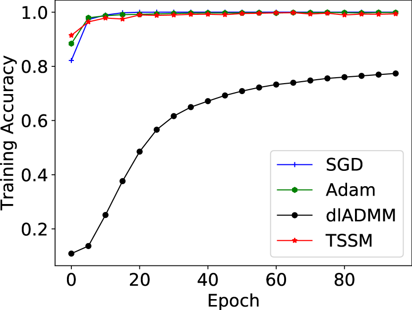
(a). MNIST

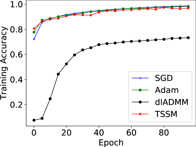
(b). Fashion MNIST

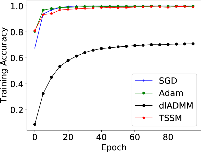
(c). kMNIST

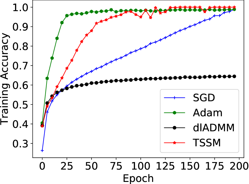
(d). CIFAR10

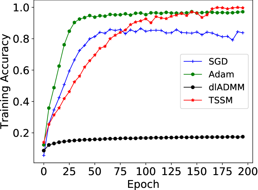
(e). CIFAR100

Figure 1: Training accuracy of all methods on five datasets. Our TSSM reaches the same training accuracy as SGD and Adam.

.

We compare the performance of the TSSM with other methods. In this experiment, we split a network into two subnetworks. gsAM performs almost identical as gsADMM, and we only shows TSSM solved by gsADMM.
We set up a feed-forward neural network which contained nine hidden layers with $512$ neurons each. The Rectified linear unit (ReLU) was used for the activation function. The loss function was set as the cross-entropy loss. $\alpha$ and $\rho$ were set to $1$. $\tau_{1}$ and $\tau_{2}$ were both set to $100$. Moreover, we set up another Convolution Neural Network (CNN), which was tested on CIFAR10 and CIFAR100 datasets. This CNN architecture has two alternating stages of $3\times 3$ convolution filters and $2\times 2$ max pooling with no stride, followed by two fully connected layer of $512$ rectified linear hidden units (ReLU’s). Each CNN layer has 32 filters. The number of epoch for feed-forward neural network and CNN was set to 100 and 200, respectively. The batch size for all methods except dlADMM was set to $120$. This is because dlADMM is a full-batch method.
As shown in Figure 1, our proposed TSSM reaches almost $100\%$ training accuracy on every dataset, which is similar to SGD and Adam. dlADMM, however, performed the worst on all datasets. This can be explained by our Theorem 1 that, dlADMM over-relaxes the neural network problems, and its performance becomes worse as the neural network gets deeper (compared with its excellent performance of shallow networks shown in [13]).

3.2.2 Speedup

(a). Training accuracy.

(b). Training time per epoch.

Figure 2: Training accuracy and training time on the ResNet-like architecture and CIFAR10 dataset: TSSM achieves the same performance as SGD yet more efficiently.

Finally, we demonstrate how much speedup the TSSM can achieve for training large-scale neural networks. We test TSSM on a ResNet-like architecture. This network consists of $9\times 9$ convolution filters with stride of 3 and $3\times 3$ max pooling with stride of 3 that are followed by 24 ResNet blocks, an average pooling and two fully connected layers of 512 rectified linear hidden units (ReLU’s). Each ResNet block is composed of two stages of $3\times 3$ convolution filters.
Figure 2(a) shows the training accuracy of SGD, Adam, and our proposed TSSM on the CIFAR10 dataset. dlADMM was not compared due to its inferior performance in the previous experiments. Specifically, we split this ResNet-like architecture into two, three, and four subnetworks. In Figure 2(a), our TSSM reaches nearly $100\%$ training accuracy for all the subnetwork configurations that we tested, while Adam only achieves below $90\%$ training accuracy. Figure 2(b) compares the training time per epoch for all methods. TSSM$\_$2, TSSM$\_$3, TSSM$\_$4 represent 2, 3, and 4 subnetworks split by TSSM, respectively. The results were the average of 500 epochs. It takes at least 40 seconds for SGD and Adam to finish an epoch, while TSSM$\_$2 only takes 25 seconds per epoch. The training duration scales (sub-linearly) as TSSM is configured with more subnetworks. TSSM can effectively reduce the training time by as much as $50\%$ without loss of training accuracy. This demonstrates TSSM’s efficacy in both training accuracy and parallelism.

4 Conclusion

In this paper, we propose the TSSM and two mode-parallelism based algorithms gsADMM and gsAM to train deep neural networks. We split a neural network into independent subnetworks while controlling the loss of performance. Experiments on five benchmark datasets demonstrate the performance and speedup of the proposed TSSM.

Appendix The defintion of Lipschitz Continuity
The Lipschitz continuity is defined as follows:

Definition 1.

(Lipschitz Continuity) A function $g(x)$ is Lipschitz continuous if there exists a constant $D>0$ such that $\forall x_{1},x_{2}$, the following holds

$$\|g(x_{1})-g(x_{2})\|\leq D\|x_{1}-x_{2}\|.$$

Proof of Theorem 1

Proof.

Because

$$\|f_{l}(W_{l},f_{l-1}(\cdots,f_{1}(W_{1},p_{1}),\cdots,))-q_{l}\|$$

$$=\|f_{l}(W_{l},f_{l-1}(\cdots,f_{1}(W_{1},p_{1}),\cdots,))-f_{l}(W_{l},p_{l})+f_{l}(W_{l},p_{l})-q_{l}\|$$

$$\leq\|f_{l}(W_{l},f_{l-1}(\cdots,f_{1}(W_{1},p_{1}),\cdots,))-f_{l}(W_{l},p_{l})\|+\|f_{l}(W_{l},p_{l})-q_{l}\|\text{ (Triangle Inequality)}$$

$$\leq H_{l}(W_{l})\|f_{l-1}(\cdots,f_{1}(W_{1},p_{1}),\cdots,)-p_{l}\|+\|f_{l}(W_{l},p_{l})-q_{l}\|(\text{$f_{l}$ is Lipschitz continuous})$$

$$=H_{l}(W_{l})\|f_{l-1}(\cdots,f_{1}(W_{1},p_{1}),\cdots,)-q_{l-1}\|+\|f_{l}(W_{l},p_{l})-q_{l}\|(\text{$q_{l-1}=p_{l}$})$$

$$=H_{l}(W_{l})\|f_{l-1}(\cdots,f_{1}(W_{1},p_{1}),\cdots,)-q_{l-1}\|+\|r_{l}\|(r_{l}=f_{l}(W_{l},p_{l})-q_{l})$$ (9)

We apply recursively Equation (9) to obtain

$$\|f_{n-1}(W_{n-1},f_{n-2}(\cdots,f_{1}(W_{1},p_{1}),\cdots,))-q_{n-1}\|$$

$$\leq H_{n-1}(W_{n-1})\|f_{n-2}(\cdots,f_{1}(W_{1},p_{1}),\cdots,)-q_{n-2}\|+\|r_{n-1}\|$$

$$\leq H_{n-1}(W_{n-1})H_{n-2}(W_{n-2})\|f_{n-3}(\cdots,f_{1}(W_{1},p_{1}),\cdots,)-q_{n-3}\|+H_{n-1}(W_{n-1})\|r_{n-2}\|+\|r_{n-1}\|$$

$$\leq\cdots$$

$$\leq\sum\nolimits_{l=1}^{n-1}(\|r_{l}\|\prod\nolimits_{j=l+1}^{n-1}H_{j}(W_{j}))$$

Therefore

$$\|R(W_{n},f_{n-1}(W_{n-1},\cdots,f_{1}(W_{1},p_{1}),\cdots,);y)-R(W_{n},p_{n};y)\|$$

$$\leq H_{n}(W_{n})\|f_{n-1}(W_{n-1},\cdots,f_{1}(W_{1},p_{1}),\cdots,)-p_{n}\|$$

$$=H_{n}(W_{n})\|f_{n-1}(W_{n-1},\cdots,f_{1}(W_{1},p_{1}),\cdots,)-q_{n-1}\|(\textbf{$q_{n-1}=p_{n}$})$$

$$\leq H_{n}(W_{n})\sum\nolimits_{l=1}^{n-1}(\|r_{l}\|\prod\nolimits_{j=l+1}^{n-1}H_{j}(W_{j}))$$

∎

Experimental Details

Dataset

In this experiment, five benchmark datasets were used for comparison, all of which are provided by the Keras library [2].
1. MNIST [9]. The MNIST dataset has ten classes of handwritten-digit images, which was firstly introduced by Lecun et al. in 1998 [9]. It contains 55,000 training samples and 10,000 test samples with 196 features each.
2. Fashion MNIST [14]. The Fashion MNIST dataset has ten classes of assortment images on the website of Zalando, which is Europe’s largest online fashion platform [14]. The Fashion-MNIST dataset consists of 60,000 training samples and 10,000 test samples with 196 features each.
3. Kuzushiji-MNIST [3]. The Kuzushiji-MNIST dataset has ten classes, each of which is a character to represent each of the 10 rows of Hiragana. The Kuzushiji-MNIST dataset consists of 60,000 training samples and 10,000 test samples with 196 features each.
4. CIFAR10 [8]. CIFAR10 is a collection of color images with 10 different classes. The number of training data and test data are 60,000 and 10,000, respectively, with 768 features each.
5. CIFAR100 [8]. CIFAR100 is similar to CIFAR10 except that CIFAR100 has 100 classes. The number of training data and test data are 60,000 and 1,0000, respectively, with 768 features each.

Comparison Methods

The SGD, Adam, and the dlADMM are state-of-the-art comparison methods. All hyperparameters were chosen by maximizing the accuracy of the training dataset.
1) Stochastic Gradient Descent (SGD) [1]. SGD and its variants are the most popular deep learning optimizers, whose convergence has been studied extensively in the literature. The learning rate was set to $10^{-2}$.
2) Adaptive momentum estimation (Adam) [7]. Adam is the most popular optimization method for deep learning models. It estimates the first and second momentum to correct the biased gradient and thus makes convergence fast. The learning rate was set to $10^{-3}$.
3) deep learning Alternating Direction Method of Multipliers (dlADMM) [13]. dlADMM is an improved version of ADMM for deep learning models. The parameter $\rho$ was set to $10^{-6}$.

References

- [1] Léon Bottou. Large-scale machine learning with stochastic gradient descent. In Proceedings of COMPSTAT’2010, pages 177–186. Springer, 2010.
- [2] François Chollet et al. Keras. https://keras.io, 2015.
- [3] Tarin Clanuwat, Mikel Bober-Irizar, Asanobu Kitamoto, Alex Lamb, Kazuaki Yamamoto, and David Ha. Deep learning for classical japanese literature. In NeurIPS 2018 Workshop on Machine Learning for Creativity and Design, 2018.
- [4] Kaiming He, Xiangyu Zhang, Shaoqing Ren, and Jian Sun. Deep residual learning for image recognition. In Proceedings of the IEEE conference on computer vision and pattern recognition, pages 770–778, 2016.
- [5] Zhouyuan Huo, Bin Gu, and Heng Huang. Training neural networks using features replay. In Advances in Neural Information Processing Systems, pages 6659–6668, 2018.
- [6] Zhouyuan Huo, Bin Gu, Heng Huang, et al. Decoupled parallel backpropagation with convergence guarantee. In International Conference on Machine Learning, pages 2098–2106, 2018.
- [7] Diederik P Kingma and Jimmy Ba. Adam: A method for stochastic optimization. 2014.
- [8] Alex Krizhevsky et al. Learning multiple layers of features from tiny images. Technical report, Citeseer, 2009.
- [9] Yann LeCun, Léon Bottou, Yoshua Bengio, Patrick Haffner, et al. Gradient-based learning applied to document recognition. Proceedings of the IEEE, 86(11):2278–2324, 1998.
- [10] Henry Leung and Simon Haykin. The complex backpropagation algorithm. IEEE Transactions on signal processing, 39(9):2101–2104, 1991.
- [11] Riccardo Miotto, Fei Wang, Shuang Wang, Xiaoqian Jiang, and Joel T Dudley. Deep learning for healthcare: review, opportunities and challenges. Briefings in bioinformatics, 19(6):1236–1246, 2018.
- [12] Aladin Virmaux and Kevin Scaman. Lipschitz regularity of deep neural networks: analysis and efficient estimation. In Advances in Neural Information Processing Systems, pages 3835–3844, 2018.
- [13] Junxiang Wang, Fuxun Yu, Xiang Chen, and Liang Zhao. Admm for efficient deep learning with global convergence. In Proceedings of the 25th ACM SIGKDD International Conference on Knowledge Discovery & Data Mining, pages 111–119, 2019.
- [14] Han Xiao, Kashif Rasul, and Roland Vollgraf. Fashion-mnist: a novel image dataset for benchmarking machine learning algorithms. 2017.
- [15] Liang Zhao, Jiangzhuo Chen, Feng Chen, Wei Wang, Chang-Tien Lu, and Naren Ramakrishnan. Simnest: Social media nested epidemic simulation via online semi-supervised deep learning. In 2015 IEEE International Conference on Data Mining, pages 639–648. IEEE, 2015.