The Fun is Finite: Douglas–Rachford and Sudoku Puzzle — Finite Termination and Local Linear Convergence

Abstract

In recent years, the Douglas–Rachford splitting method has been shown to be effective at solving many non-convex optimization problems. In this paper we present a local convergence analysis for non-convex feasibility problems and show that both finite termination and local linear convergence are obtained. For a generalization of the Sudoku puzzle, we prove that the local linear rate of convergence of Douglas–Rachford is exactly $\frac{\sqrt{5}}{5}$ and independent of puzzle size. For the $s$-queens problem we prove that Douglas–Rachford converges after a finite number of iterations. Numerical results on solving Sudoku puzzles and $s$-queens puzzles are provided to support our theoretical findings.

Key words. Douglas–Rachford $\cdot$ Feasibility problem $\cdot$ Sudoku Puzzle $\cdot$ Finite Termination Local Linear Convergence

AMS subject classifications. 49J52 $\cdot$ 65K05 $\cdot$ 65K10 $\cdot$ 90C25

1 Introduction

Given two non-empty sets $C$ and $S$ whose intersection is also non-empty, the feasibility problem aims to find a common point in the intersection $C\cap S$. In the literature, popular numerical schemes for solving feasibility problems are developed based on projection, among them alternating projection is the fundamental one. The method of alternating projection was first introduced by von Neumann for the case of two linear subspaces [29], then was extended to closed convex sets by Bregman [11]. Relaxation is a standard approach to speed up alternating projection and related work can be found in [22, 12].

Proximal splitting methods, such as Forward–Backward [21] splitting and Backward–Backward splitting [13], and Peaceman–Rachford/Douglas–Rachford splitting [25, 14], can also be applied to solve feasibility problem either directly or up to reformulation. Moreover, equivalence between projection based methods and proximal splitting methods can be established, such as alternating projection is equivalent to Backward–Backward splitting while relaxed alternating relaxed projection covers Peaceman–Rachford/Douglas–Rachford splitting as special cases [13].

Our focus in this paper is Douglas-Rachford splitting method, which has shown to be effective for solving feasibility problem, particularly in the non-convex setting [7]. However, the convergence property is rather less understood than its convex counter part. One reason for this is that Douglas–Rachford splitting method is not symmetric and non-descent, when compared to (proximal) gradient descent whose non-convex case is much better studied [4]. Research on non-convex Douglas–Rachford either focuses on specific cases or imposing stronger assumptions (e.g. smoothness) and proposes modifications to the original iteration. For instance [1] considers Douglas–Rachford splitting for solving feasibility problem of a line intersecting with a circle, and conditions for convergence are provided. In [19], the authors proposed a damped Douglas–Rachford splitting method for general non-convex optimization problem under the condition that one function has a Lipschitz continuous gradient.

The study of this paper is motivated by applying Douglas–Rachford to solve Sudoku puzzle, for which three different convergence behaviors are observed

• Globally, the method converges sub-linearly.

• Locally, two regimes occur: finite termination and linear convergence.

Finite termination and local linear convergence are reported in the literature [10, 7], however, conditions in respective work either are designed for convex setting or cannot be satisfied by Sudoku puzzle. Therefore, a new analysis is needed for Douglas–Rachford splitting which is the aim of this paper:

1. Finite termination Under a non-degeneracy condition, see (4.1), we show in Section 4 that one sequence generated by Douglas–Rachford splitting has the finite termination property. All sequences terminate in a finite number of iterations if the problem satisfies certain assumptions (e.g. polyhedrality, see Assumptions A.1-A.3).

2. Local linear convergence We also provide a precise characterization for the local linear convergence of Douglas–Rachford splitting method. Particularly, for Sudoku puzzle, we prove that locally the linear rate of convergence of Douglas–Rachford splitting method is precisely $\frac{\sqrt{5}}{5}$. Moreover, such a rate is independent of puzzle size. For the damped Douglas–Rachford splitting method, we also provide an exact estimation of the local linear rate which depends on the damping coefficient.

Relation to Prior Work

There are several existing work studying the finite termination property of the standard Douglas–Rachford splitting method. In [10], the authors established finite convergence of Douglas–Rachford in the presence of Slater’s condition, for solving convex feasibility problems where one set is an affine subspace and the other is a polyhedron, or one set is an epigraph and the other one is a hyperplane. The result was extended to general convex optimization problems in [20] under the notion of partial smoothness [18]. In [23], finite termination is proved for finding a point which is guaranteed to be in the interior of one set whose interior is assumed to be non-empty. The result of [10] was later extended to the non-convex case in [7], where one of the two sets can be finite.

For local linear convergence, results can be found in for instance [26] where linear convergence of Douglas–Rachford splitting method is established under a regularity condition. Similar results can be found in [16, 15]. Under a constraint qualification condition, [19] also discussed the local linear convergence property of the damped Douglas–Rachford splitting method.

Paper Organization

The rest of the paper is organized as follows. Some preliminaries are collected in Section 2. Section 3 states our main assumptions on problem (3.1) and introduces the standard and damped Douglas–Rachford algorithms, global convergence is also discussed. Our main result on local convergence of Douglas–Rachford is presented in Section 4. In Section 5, we report numerical experiments on Sudoku puzzle and $s$-queens puzzle to support our theoretical findings.

2 Preliminaries

Throughout the paper, $\mathbb{N}$ is the set of nonnegative integers, $\mathbb{R}^{n}$ is a finite $n$-dimensional real Euclidean space equipped with scalar product $\langle\cdot,\,\cdot\rangle$ and norm ${|\kern-1.125pt|}\cdot{|\kern-1.125pt|}$. $\mathrm{Id}$ denotes the identity operator on $\mathbb{R}^{n}$. For a matrix $M\in\mathbb{R}^{n\times n}$, we denote $\rho(M)$ its spectral radius.

Projection and reflection

Below we collect necessary concepts related to sets.

Definition 2.1 (Distance and indicator function).

Let $C\subset\mathbb{R}^{n}$ be non-empty and $x\in\mathbb{R}^{n}$. The distance function of $x$ to $C$ is defined by

$$\mathrm{dist}(x,C)\stackrel{{\scriptstyle{\mathrm{def}}}}{{=}}\inf_{y\in C}{|\kern-1.125pt|}x-y{|\kern-1.125pt|}.$$

The indicator function of $C$ is defined by $\iota_{C}(x)=\left\{\begin{aligned} 0&:x\in C,\\ +\infty&:x\notin C.\end{aligned}\right.$

Definition 2.2 (Projection & reflection).

Let $C\subset\mathbb{R}^{n}$ be non-empty and $x\in\mathbb{R}^{n}$. The projection of $x$ onto $C$, denoted by $\mathscr{P}_{C}(x)$, is a set defined by

$$\mathscr{P}_{C}(x)\stackrel{{\scriptstyle{\mathrm{def}}}}{{=}}\big{\{}y\in C:{|\kern-1.125pt|}x-y{|\kern-1.125pt|}=\mathrm{dist}(x,C)\big{\}}.$$

The mapping $\mathscr{P}_{C}\colon\mathbb{R}^{n}\rightrightarrows C$ is called the projection operator. The relaxed projection $\mathscr{P}^{\lambda}_{C}$ is defined via

$$\mathscr{P}^{\lambda}_{C}(x)=\lambda\mathscr{P}_{C}(x)+(1-\lambda)x,$$

where $\lambda\in]0,2]$ is the relaxation parameter. When $\lambda=2$, the corresponding mapping is called reflection and denoted by $\mathscr{R}_{C}(x)=2\mathscr{P}_{C}(x)-x$.

Definition 2.3 (Prox-regularity).

A non-empty closed set $C\subset\mathbb{R}^{n}$ is prox-regular at $x\in C$ for $v$ if $x=\mathscr{P}_{C}(x+v)$. If $\mathscr{P}_{C}$ is single-valued in an open neighborhood of $x\in C$, $C$ is called prox-regular at $x$.

Definition 2.4 (Normal vector).

Given $C\subset\mathbb{R}^{n}$ and $x\in C$, the proximal normal cone $\mathscr{N}_{C}^{p}(x)$ of $C$ at $x$ is defined by

$$\mathscr{N}_{C}^{p}(x)=\mathrm{cone}\big{(}{\mathscr{P}_{C}^{-1}(x)-x}\big{)}.$$

The limiting normal cone $\mathscr{N}_{C}(x)$ is defined as any vector that can be written as the limit of proximal normals: $v\in\mathscr{N}_{C}(x)$ if and only if there exists sequences $\{x_{k}\}_{k\in\mathbb{N}}\in C$ and $\{v_{k}\}_{k\in\mathbb{N}}$ in $\mathscr{N}_{C}(x_{k})$ such that $x_{k}\to x$ and $v_{k}\to v$.

Let $C_{1},C_{2}\subset\mathbb{R}^{n}$ be two sets with non-empty intersection. The feasibility problem of $C_{1},C_{2}$ is to find a common point in the intersection, i.e.

$$\mathrm{find}\quad x\in\mathbb{R}^{n}\quad\mathrm{s.t.}\quad x\in C_{1}\mathbin{\scalebox{1.5}{$\cap$}}C_{2}.$$

A fundamental algorithm to solve the problem is the alternating projection method which, as indicated by the name, represents the procedure: from a given point $x_{0}$, apply projection onto each set alternatively

$$x_{k+1}=\mathscr{P}_{C_{2}}\mathscr{P}_{C_{1}}(x_{k}).$$ (2.1)

One can also consider relaxation for each projection operator and the whole iteration, which results in the following iteration

$$x_{k+1}=x_{k}+\lambda\big{(}{\mathscr{P}^{\lambda_{2}}_{C_{2}}\mathscr{P}^{\lambda_{1}}_{C_{1}}(x_{k})-x_{k}}\big{)},$$

where $\lambda,{\lambda_{1}},{\lambda_{2}}$ are relaxation parameters. The iteration becomes Peaceman–Rachford splitting (alternating reflection) for $(\lambda,{\lambda_{1}},{\lambda_{2}})=(1,2,2)$ and Douglas–Rachford splitting for $(\lambda,{\lambda_{1}},{\lambda_{2}})=(1/2,2,2)$. We refer to [6] for a survey on the alternating projection method.

Convergent Matrices

To discuss the local linear convergence, we need the following preliminary results on convergent matrices which are taken from [24].

Definition 2.5 (Convergent matrices).

A matrix $M\in\mathbb{R}^{n\times n}$ is convergent to $\mathrm{M}^{\infty}\in\mathbb{R}^{n\times n}$ if, and only if, $\lim_{k\to+\infty}{|\kern-1.125pt|}M^{k}-\mathrm{M}^{\infty}{|\kern-1.125pt|}=0$. $M$ is said to be linearly convergent if there exists $\eta\in[0,1[$ and $K\in\mathbb{N}$ such that for all $k\geq K$, there holds ${|\kern-1.125pt|}M^{k}-\mathrm{M}^{\infty}{|\kern-1.125pt|}=O(\eta^{k})$. If $M$ does not converge at any rate $\eta^{\prime}\in[0,\eta[$ then $\eta$ is called the optimum convergence rate.

Definition 2.6 (Semi-simple eigenvalue).

For $M\in\mathbb{R}^{n\times n}$, an eigenvalue $\eta$ is called semi-simple if and only if $\mathrm{rank}(M-\eta\mathrm{Id})=\mathrm{rank}((M-\eta\mathrm{Id})^{2})$.

Theorem 2.7 (Limits of powers).

For $M\in\mathbb{R}^{n\times n}$, the power of $M$ converges to $\mathrm{M}^{\infty}$ if and only if $\rho(M)<1$ or $\rho(M)=1$ with $1$ being the only eigenvalue on the complex unit circle and semi-simple.

Whenever $M$ is convergent, it converges linearly to $\mathrm{M}^{\infty}$, and we have the following lemma.

Lemma 2.8 (Convergence rate).

Suppose $M\in\mathbb{R}^{n\times n}$ is convergent to some $\mathrm{M}^{\infty}\in\mathbb{R}^{n\times n}$, then

1. for any $k\in\mathbb{N}$,

   $$M^{k}-\mathrm{M}^{\infty}=(M-\mathrm{M}^{\infty})^{k}\quad\text{and}\quad{|\kern-1.125pt|}M^{k}-\mathrm{M}^{\infty}{|\kern-1.125pt|}\leq{|\kern-1.125pt|}M-\mathrm{M}^{\infty}{|\kern-1.125pt|}^{k}.$$

   The equality holds only when $M$ is normal.

2. We have $\rho(M-\mathrm{M}^{\infty})<1$, and $M$ is linearly convergent for any $\eta\in]\rho(M-\mathrm{M}^{\infty}),1[$.

3. $\rho(M-\mathrm{M}^{\infty})$ is the optimal convergence rate if one of the following holds

   1. $M$ is normal.

   2. All the eigenvalues $\eta\in\Theta_{M}$ such that ${\lvert}\eta{\rvert}=\rho(M-\mathrm{M}^{\infty})$ are semi-simple.

• See Theorems 2.12, 2.13, 2.15 and 2.16 of [9]. ∎

Angles between Subspaces

To precisely characterize the local linear convergence rate, we need the following concepts regarding the angles between subspaces. Let $T_{1}$ and $T_{2}$ be two linear subspaces with dimension $p\stackrel{{\scriptstyle{\mathrm{def}}}}{{=}}\dim(T_{1})$ and $q\stackrel{{\scriptstyle{\mathrm{def}}}}{{=}}\dim(T_{2})$, and without loss of generality, suppose that $1\leq p\leq q\leq n-1$.

Definition 2.9 (Principal angles).

The principal angles $\theta_{k}\in[0,\frac{\pi}{2}]$, $k=1,\ldots,p$ between linear subspaces $T_{1}$ and $T_{2}$ are defined by, with $u_{0}=v_{0}\stackrel{{\scriptstyle{\mathrm{def}}}}{{=}}0$ and inductively

$$\cos(\theta_{k})\stackrel{{\scriptstyle{\mathrm{def}}}}{{=}}\langle u_{k},\,v_{k}\rangle=\max\big{\{}\langle u,\,v\rangle\,\,\,\mathrm{s.t.}\,\,\, u\in T_{1},v\in T_{2},{|\kern-1.125pt|}u{|\kern-1.125pt|}=1,{|\kern-1.125pt|}v{|\kern-1.125pt|}=1,$$

$$\langle u,\,u_{i}\rangle=\langle v,\,v_{i}\rangle=0,\,i=0,\dotsm,k-1\big{\}}.$$

The principal angles $\theta_{k}$ are unique with $0\leq\theta_{1}\leq\theta_{2}\leq\dotsm\leq\theta_{p}\leq\pi/2$.

Definition 2.10 (Friedrichs angle).

The Friedrichs angle $\theta_{F}\in[0,\frac{\pi}{2}]$ between $T_{1}$ and $T_{2}$ is

$$\cos\big{(}{\theta_{F}(T_{1},T_{2})}\big{)}\stackrel{{\scriptstyle{\mathrm{def}}}}{{=}}\max\langle u,\,v\rangle\,\,\,\mathrm{s.t.} u\in T_{1}\cap(T_{1}\cap T_{2})^{\perp},{|\kern-1.125pt|}u{|\kern-1.125pt|}=1,$$

$$v\in T_{2}\cap(T_{1}\cap T_{2})^{\perp},{|\kern-1.125pt|}v{|\kern-1.125pt|}=1.$$

The following lemma shows the relation between the Friedrichs and principal angles.

Lemma 2.11 ([9, Proposition 3.3]).

We have $\theta_{F}(T_{1},T_{2})=\theta_{d+1}>0$ where $d\stackrel{{\scriptstyle{\mathrm{def}}}}{{=}}\dim(T_{1}\cap T_{2})$.

3 Problem and algorithm

The formal statement of the feasibility problem is written below

$$\mathrm{find}\quad\,\,{x\in\mathbb{R}^{n}}\quad\mathrm{s.t.}\quad x\in C\mathbin{\scalebox{1.5}{$\cap$}}S,$$ (3.1)

where the following assumptions are imposed

1. $C\subset\mathbb{R}^{n}$ is a closed set;

2. $S\subset\mathbb{R}^{n}$ is an affine subspace;

3. $C\mathbin{\scalebox{1.5}{$\cap$}}S\neq\emptyset$, i.e. the intersection is non-empty.

Note that the problem (3.1) is not necessarily convex as we suppose $C$ is only non-empty and closed. Examples of (3.1) are provided in Section 4, including the Sudoku puzzle and $s$-queens puzzle.

3.1 Douglas–Rachford splitting method

The development of Douglas–Rachford (DR) splitting method [14] dates back to 1950s for solving numerical PDEs. In recently years, the method has also been shown to be effective for non-convex feasibility problem [17, 2]. Details of the method for solving (3.1) is described in Algorithm 1.

Initial: $z_{0}\in\mathbb{R}^{n}$;

repeat

      

$$x_{k+1} =\mathscr{P}_{S}({z}_{k}),$$ (3.2)

$$u_{k+1} \in\mathscr{P}_{C}(2x_{k+1}-{z}_{k}),$$

$${z}_{k+1} ={z}_{k}+u_{k+1}-x_{k+1},$$

until convergence;

Algorithm 1 Standard Douglas–Rachford splitting (DR)

The above iteration can be written as the fixed-point iteration of variable ${z}_{k}$. Denote the fixed-point operator

$$\mathscr{F}_{\mathrm{DR}}\stackrel{{\scriptstyle{\mathrm{def}}}}{{=}}{{\frac{\raisebox{0.41669pt}{\footnotesize$1$}}{\raisebox{-1.24994pt}{\footnotesize$2$}}}}\big{(}{(2\mathscr{P}_{C}-\mathrm{Id})(2\mathscr{P}_{S}-\mathrm{Id})+\mathrm{Id}}\big{)},$$ (3.3)

then we have ${z}_{k+1}=\mathscr{F}_{\mathrm{DR}}({z}_{k})$. The other two variables $u_{k},x_{k}$ are called the shadow sequences [8].

Determining the convergence properties of Douglas–Rachford splitting for the non-convex setting is a challenging problem, the non-descent property of the method makes it much harder to obtain convergence result than the descent-type methods which includes (proximal) gradient descent [4].

Moreover, since the method has three different sequences $u_{k},x_{k}$ and ${z}_{k}$, various different convergence behaviors may occur. We refer to [7] for more detailed discussions. In Example 3.2, we demonstrate a case of a circle intersecting with a line where:

• The shadow sequences $\{u_{k}\}_{k\in\mathbb{N}}$, $\{x_{k}\}_{k\in\mathbb{N}}$ converge to $u^{\star}$ and $x^{\star}$, respectively. But $u^{\star}\neq x^{\star}$.

• The fixed-point sequence $\{{z}_{k}\}_{k\in\mathbb{N}}$ diverges.

As our main interest in this paper is to study the local behavior, for the rest of the paper, we suppose that the standard DR is globally convergent:

1. The standard Douglas–Rachford splitting method for solving (3.1) is globally convergent.

Consequently, one has

$${z}_{k}\to{z}^{\star}\in\mathrm{Fix}(\mathscr{F}_{\mathrm{DR}})\stackrel{{\scriptstyle{\mathrm{def}}}}{{=}}\big{\{}z\in\mathbb{R}^{n}:z=\mathscr{F}_{\mathrm{DR}}(z)\big{\}}\quad\text{and}\quad u_{k},x_{k}\to x^{\star}\in\mathscr{P}_{S}({z}^{\star}).$$

To avoid assumption (A.4), people either turn to specific cases [3] or imposing stronger assumptions such as smoothness [28]. Modifications to the original Douglas–Rachford splitting method are also considered in the literature. Below we describe a damped version of Douglas–Rachford proposed in [19].

Solving the feasibility problem (3.1) is equivalent to the following constrained smooth optimization.

$$\min_{x\in\mathbb{R}^{n}}\,{{\frac{\raisebox{0.41669pt}{\footnotesize$1$}}{\raisebox{-1.24994pt}{\footnotesize$2$}}}}\mathrm{dist}^{2}(x,S)\,\quad\mathrm{s.t.}\quad x\in C.$$ (3.4)

In (3.2), the update of $x_{k+1}$ is equivalent to solving $\min_{x\in\mathbb{R}^{n}}\,\iota_{S}(x)+\frac{1}{2\gamma}{|\kern-1.125pt|}x-{z}_{k}{|\kern-1.125pt|}^{2}$. Replacing the indicator function with the distance function,

$$\min_{x\in\mathbb{R}^{n}}\,{{\frac{\raisebox{0.41669pt}{\footnotesize$1$}}{\raisebox{-1.24994pt}{\footnotesize$2$}}}}\mathrm{dist}^{2}(x,S)+{{\frac{\raisebox{0.41669pt}{\footnotesize$1$}}{\raisebox{-1.24994pt}{\footnotesize$2\gamma$}}}}{|\kern-1.125pt|}x-{z}_{k}{|\kern-1.125pt|}^{2},$$

we then get

$$x_{k+1}={{\frac{\raisebox{0.41669pt}{\footnotesize$1$}}{\raisebox{-1.24994pt}{\footnotesize$1+\gamma$}}}}\big{(}{{{z}_{k}}+\gamma\mathscr{P}_{S}({z}_{k})}\big{)}={z}_{k}+{{\frac{\raisebox{0.41669pt}{\footnotesize$\gamma$}}{\raisebox{-1.24994pt}{\footnotesize$1+\gamma$}}}}\big{(}{\mathscr{P}_{S}({z}_{k})-{z}_{k}}\big{)}=\mathscr{P}_{S}^{\frac{\gamma}{1+\gamma}}({z}_{k}).$$

As a result, we obtain the algorithm proposed in [19].

Initial: $\gamma>0$, $z_{0}\in\mathbb{R}^{n}$;

repeat

      

$$x_{k+1} =\mathscr{P}_{S}^{\frac{\gamma}{1+\gamma}}({z}_{k}),$$ (3.5)

$$u_{k+1} \in\mathscr{P}_{C}(2x_{k+1}-{z}_{k}),$$

$${z}_{k+1} ={z}_{k}+u_{k+1}-x_{k+1},$$

until convergence;

Algorithm 2 A damped Douglas–Rachford splitting (dDR)

We refer to the original work [19] for a more detailed discussion of Algorithm 2. When $\gamma=+\infty$, Algorithm 2 recovers the standard Douglas–Rachford splitting method (3.2). The fixed-point operator of dDR reads

$$\mathscr{F}_{\mathrm{dDR}}\stackrel{{\scriptstyle{\mathrm{def}}}}{{=}}{{\frac{\raisebox{0.41669pt}{\footnotesize$1$}}{\raisebox{-1.24994pt}{\footnotesize$2$}}}}\big{(}{(2\mathscr{P}_{C}-\mathrm{Id})(2\mathscr{P}_{S}^{\frac{\gamma}{1+\gamma}}-\mathrm{Id})+\mathrm{Id}}\big{)}.$$ (3.6)

We have the following convergence result of dDR from [19].

Lemma 3.1 (Global convergence of dDR [19, Theorem 5]).

For the non-convex feasibility problem (3.1), suppose Assumptions A.1-A.3 hold and moreover $C$ is compact. Choose $\gamma\in]0,\sqrt{3/2}-1[$ for the Douglas–Rachford splitting method (3.5), then the sequence $\{u_{k},x_{k},{z}_{k}\}_{k\in\mathbb{N}}$ is bounded, and given any cluster point $(u^{\star},x^{\star},{z}^{\star})$ of the sequence, there holds ${|\kern-1.125pt|}{z}_{k}-{z}_{k-1}{|\kern-1.125pt|}\to 0$, $u^{\star}=x^{\star}$ and $x^{\star}$ is a stationary point of the problem (3.4).

In the example below, we demonstrate a case where DR fails to solve the problem while dDR succeeds.

Example 3.2 (A circle intersects with a line).

Let $C=\{x\in\mathbb{R}^{2}:{|\kern-1.125pt|}x{|\kern-1.125pt|}=1\}$ be the unit circle and $S=\{x\in\mathbb{R}^{2}:\langle x,\,\left(\begin{smallmatrix}1\\ 2\end{smallmatrix}\right)\rangle=\sqrt{2}\}$ be a line that intersects with $C$ at two different points. For both methods, same initial point $z_{0}=(-10,-8)$ is chosen. For damped DR, we set $\gamma=\frac{1}{5}$. In Figure 1 we observe:

• For the standard DR (left): ${z}_{k}$ is not convergent, $u_{k}$ and $x_{k}$ converge to two different points and the method fails to find a feasible point.

• For the damped DR (right): all three sequences converge to the same feasible point.

We refer to [1] for a detailed discussion of the convergence properties of the standard DR for solving this feasibility problem.

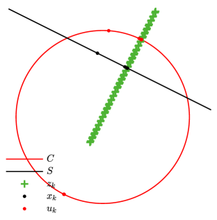
(a) Standard Douglas–Rachford

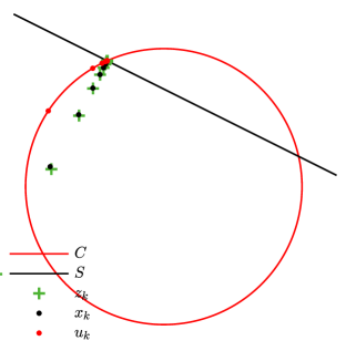
(b) Damped Douglas–Rachford

Figure 1: Convergence behavior of the standard and damped Douglas–Rachford for solving the problem of a line intersecting with a circle.

Though dDR solves the problem, as remarked in the original paper [19], it may also converges to some stationary point of (3.4) which is not a solution. In fact, as we shall see in the numerical experiments, for the Sudoku puzzle and $s$-queens puzzle, dDR with $\gamma=\frac{1}{5}\in]0,\sqrt{3/2}-1[$ fails all tests while sDR achieves very good performance; see Table 1.

3.2 Problems with more than two sets

Up to now, we have been dealing with feasibility problem of two sets, while in various scenarios we need to deal with the case of finding common points of more than two sets. In what follows, we briefly show that, by a product space trick, we can reformulate the problem into the form of (3.1).

Let $m\geq 2$ be an integer, $C_{i}$ a non-empty closed set for each $i\in\{1,\ldots,m\}$. Consider the following feasibility problem

$$\mathrm{find}\quad x\,\in\mathbb{R}^{n}\quad\mathrm{s.t.}\quad x\in\mathbin{\scalebox{1.5}{$\cap$}}_{i=1}^{m}C_{i}.$$ (3.7)

Let $\mathbfcal{H}=\underset{\textrm{$m$ times}}{\underbrace{\mathbb{R}^{n}\times\cdots\times\mathbb{R}^{n}}}$ be the product space endowed with the scalar inner-product and norm

$$\forall\bm{x},\bm{y}\in\mathbfcal{H},\,\bm{\langle\kern-5.0pt\langle}\bm{x},\bm{y}\bm{\rangle\kern-5.0pt\rangle}=\mathbin{\scalebox{1.125}{$\sum$}}_{i=1}^{m}\langle x_{i},\,y_{i}\rangle,\,\bm{|\kern-1.125pt|}\bm{x}\bm{|\kern-1.125pt|}=\big{(}{\mathbin{\scalebox{0.9}{$\sum$}}_{i=1}^{m}{|\kern-1.125pt|}x_{i}{|\kern-1.125pt|}^{2}}\big{)}^{1/2}.$$

Let $\mathbfcal{C}\stackrel{{\scriptstyle{\mathrm{def}}}}{{=}}C_{1}\times\dotsm\times C_{m}$, then $\mathbfcal{C}\subset\mathbfcal{H}$, and denote the subspace $\mathbfcal{S}\stackrel{{\scriptstyle{\mathrm{def}}}}{{=}}\{\bm{x}=(x_{i})_{i}\in\mathbfcal{H}:x_{1}=\dotsm=x_{m}\}$. The feasibility problem (3.7) can be reformulated into the following form

$$\mathrm{find}\quad\bm{x}\in\mathbfcal{H}\quad\mathrm{s.t.}\quad\bm{x}\in\mathbfcal{C}{\mathbin{\scalebox{1.5}{$\cap$}}}\mathbfcal{S}.$$ (3.8)

The projection operator of $\mathbfcal{C}$ is component-wise for each set $C_{i},i=1,\ldots,m$,

$$\mathscr{P}_{\mathbfcal{C}}\bm{x}=(\mathscr{P}_{C_{1}}x_{1},\dotsm,\mathscr{P}_{C_{m}}x_{m}).$$

Define $\mathbfcal{K}:\mathbb{R}^{n}\to\mathbfcal{S},\,x\mapsto(x,\dotsm,x)$, then we have $\mathscr{P}_{\mathbfcal{S}}(\bm{x})=\mathbfcal{K}(\tfrac{1}{m}\sum_{i=1}^{m}x_{i})$.

Adapting the standard Douglas–Rachford to the case of (3.7), we obtain

$$x_{k+1}={{\frac{\raisebox{0.41669pt}{\footnotesize$1$}}{\raisebox{-1.24994pt}{\footnotesize$m$}}}}\mathbin{\scalebox{1.125}{$\sum$}}_{i=1}^{m}z_{i,k},$$ (3.9)

For $$i=1,\ldots,m$$:

$$\left\lfloor\begin{aligned} u_{i,k+1}&\in\mathscr{P}_{C_{i}}(2x_{k+1}-z_{i,k}),\\ z_{i,k+1}&=z_{i,k}+u_{i,k+1}-x_{k+1}.\end{aligned}\right.$$

Note that for the standard DR, there is no need to store $\bm{x}$ and simply $x_{k+1}=\frac{1}{m}\mathbin{\scalebox{1.125}{$\sum$}}_{i=1}^{m}z_{i,k}$ is sufficient. Correspondingly, we also have the following iteration for the damped Douglas–Rachford splitting method:

For $$i=1,\ldots,m$$: (3.10)

$$\left\lfloor\begin{aligned} x_{i,k+1}&={{\frac{\raisebox{0.41669pt}{\footnotesize$1$}}{\raisebox{-1.24994pt}{\footnotesize$1+\gamma$}}}}\big{(}{z_{i,k}+\gamma{{\frac{\raisebox{0.41669pt}{\footnotesize$1$}}{\raisebox{-1.24994pt}{\footnotesize$m$}}}}\mathbin{\scalebox{1.125}{$\sum$}}_{j=1}^{m}z_{j,k}}\big{)},\\ u_{i,k+1}&\in\mathscr{P}_{C_{i}}(2x_{i,k+1}-z_{i,k}),\\ z_{i,k+1}&=z_{i,k}+u_{i,k+1}-x_{i,k+1}.\end{aligned}\right.$$

4 Local convergence of Douglas–Rachford splitting

In this section we present our main result, the local convergence of Douglas–Rachford splitting. We first present the result in a general setting and then specialize to the case of Sudoku and $s$-queens puzzles.

Non-degeneracy condition

To deliver the result, a non-degeneracy condition is needed for set $C$. Assume Assumption A.4 holds for standard DR and that dDR is ran under the condition of Lemma 3.1, then at convergence for both methods we have ${z}_{k}\to{z}^{\star}$ and $u_{k},x_{k}\to x^{\star}$. We assume that $C$ is prox-regular at $x^{\star}$ for $x^{\star}-{z}^{\star}$ and the following condition holds

$$x^{\star}-{z}^{\star}\in\mathrm{int}\big{(}{\mathscr{N}_{C}(x^{\star})}\big{)}$$ (4.1)

where $\mathrm{int}(\cdot)$ stands for the interior of the set.

Remark 4.1.

The non-degeneracy condition (4.1) requires $\mathscr{N}_{C}(x^{\star})$ has a non-empty interior, which means that $x^{\star}$ is a vertex of the set $C$. A graphical illustration of the non-degeneracy condition (4.1) is provided in Figure 2 below.

Figure 2: Normal cone (red) at a point $x^{*}$ in the polytope $C$ (green).

4.1 Local convergence of Douglas–Rachford splitting

We start with the standard Douglas–Rachford splitting and then the damped iteration. Relation with some existing work in the literature is also discussed.

4.1.1 The standard Douglas–Rachford splitting

For standard Douglas–Rachford splitting method, for what follows we impose the global convergence as an assumption, i.e. A.4 holds.

Theorem 4.2 (Finite termination of DR).

For the feasibility problem (3.1) and the Douglas–Rachford iteration (3.2), suppose Assumptions A.1-A.4 hold. Then $\{u_{k},x_{k},{z}_{k}\}_{k\in\mathbb{N}}$ converges to $(x^{\star},x^{\star},{z}^{\star})$ with ${z}^{\star}\in\mathrm{Fix}(\mathscr{F}_{\mathrm{DR}})$ being a fixed point and $x^{\star}=\mathscr{P}_{S}({z}^{\star})$. If, moreover, the non-degeneracy condition (4.1) holds, then $\{u_{k},x_{k},{z}_{k}\}_{k\in\mathbb{N}}$ converges to $(x^{\star},x^{\star},{z}^{\star})$ finitely.

Remark 4.3.

It is worth noting that Theorem 4.2 also holds true for the convex setting. In [10] the authors study DR for solving convex affine-polyhedral feasibility problem, and impose the following condition for finite convergence

$$S\mathbin{\scalebox{1.5}{$\cap$}}\mathrm{int}(C)\neq\emptyset,$$ (4.2)

which does not hold for the non-convex case as the interior of $C$ in (3.1) can be empty; See also Section 4.2 the puzzles for which (4.2) fails. In [7], when the non-convex set is finite, finite termination is proved given that the other set is an affine subspace or a half-space. In comparison, our result here does not need the set to be finite and provides an extension to that of [10], as we characterize the situation where finite convergence happens but (4.2) fails.

• The imposed global convergence of (3.2) means

  $${z}_{k}\to{z}^{\star}\in\mathrm{Fix}(\mathscr{F}_{\mathrm{DR}})\quad\text{and}\quad u_{k},x_{k}\to x^{\star}=\mathscr{P}_{S}({z}^{\star}).$$ (4.3)

  The prox-regularity of $C$ at $x^{\star}$ for $x^{\star}-{z}^{\star}$ and the non-degeneracy condition (4.1) imply that there exists an open set $\mathcal{B}$ such that

  $$2x^{\star}-{z}^{\star}\in\mathcal{B}\subset\mathscr{N}_{C}(x^{\star})+x^{\star}\quad\text{and}\quad\mathscr{P}_{C}(\mathcal{B})=\{x^{\star}\}.$$

  By the definition of convergence, there must therefore exist $K\in\mathbb{N}$ such that $2x_{k+1}-{z}_{k+1}\in\mathcal{B}$ for all $k\geq K$. Consequently, by the update of $u_{k+1}$ in (3.5),

  $$u_{k+1}=\mathscr{P}_{C}(2x_{k+1}-{z}_{k})=x^{\star}$$

  which is the finite convergence of $u_{k+1}$.

  For the update of $x_{k}$ in (3.2), this time we have directly

  $$x_{k+1}-x^{\star} =\mathscr{P}_{S}({z}_{k}-{z}^{\star}).$$

  For ${z}_{k+1}$, let $K>0$ be such that $u_{k}=x^{\star}$ for all $k\geq K$, we have

  $${z}_{k+1}-{z}^{\star}=({z}_{k}-{z}^{\star})+(u_{k+1}-x^{\star})-(x_{k+1}-x^{\star}) =({z}_{k}-{z}^{\star})-(x_{k+1}-x^{\star})$$

  $$=(\mathrm{Id}-\mathscr{P}_{S})({z}_{k}-{z}^{\star})$$

  $$=(\mathrm{Id}-\mathscr{P}_{S})^{k+1-K}(z_{K}-{z}^{\star}).$$

  Since ${z}_{k}\to{z}^{\star}$ and $(\mathrm{Id}-\mathscr{P}_{S})^{k+1-K}=\mathrm{Id}-\mathscr{P}_{S}$, we have

  $$0=\lim_{k\to+\infty}{z}_{k+1}-{z}^{\star}=\lim_{k\to+\infty}(\mathrm{Id}-\mathscr{P}_{S})^{k+1-K}(z_{K}-{z}^{\star}) =(\mathrm{Id}-\mathscr{P}_{S})(z_{K}-{z}^{\star})={z}_{k+1}-{z}^{\star},$$

  which means ${z}_{k}={z}^{\star}$ for all $k>K$, hence finite termination of ${z}_{k}$. The finite convergence of $x_{k}$ follows naturally that of ${z}_{k}$, and we conclude the proof. ∎

Different order of update

In (3.2), the order of the projection operators can be switched which results in the following iteration

$$x_{k+1} \in\mathscr{P}_{C}({z}_{k}),$$ (4.4)

$$u_{k+1} =\mathscr{P}_{S}(2x_{k+1}-{z}_{k}),$$

$${z}_{k+1} ={z}_{k}+u_{k+1}-x_{k+1}.$$

The corollary below shows that the finite termination holds for (4.4).

Corollary 4.4.

For the feasibility problem (3.1) and the Douglas–Rachford iteration (4.4), suppose Assumptions A.1-A.4 hold. Then $\{u_{k},x_{k},{z}_{k}\}_{k\in\mathbb{N}}$ converges to $(x^{\star},x^{\star},{z}^{\star})$ with ${z}^{\star}\in\mathrm{Fix}(\mathscr{F}_{\mathrm{DR}})$ being a fixed point and $x^{\star}\in\mathscr{P}_{C}({z}^{\star})$. If, moreover, $C$ is prox-regular at $x^{\star}$ for ${z}^{\star}-x^{\star}$ and the following non-degeneracy condition holds,

$$-(x^{\star}-{z}^{\star})\in\mathrm{int}\big{(}{\mathscr{N}_{C}(x^{\star})}\big{)},$$ (4.5)

then $\{u_{k},x_{k},{z}_{k}\}_{k\in\mathbb{N}}$ converges to $(x^{\star},x^{\star},{z}^{\star})$ in a finite number of iterations.

• Following the argument of the proof of Theorem 4.2, we can easily derive the finite termination of $x_{k}$ under the new non-degeneracy condition (4.5). In turn, for $k$ large enough, we have for $u_{k+1}$ that

  $$u_{k+1}-x^{\star} =\mathscr{P}_{S}(2x_{k+1}-{z}_{k})-\mathscr{P}_{S}(2x^{\star}-{z}^{\star})$$

  $$=2\mathscr{P}_{S}(x_{k+1}-x^{\star})-\mathscr{P}_{S}({z}_{k}-{z}^{\star})$$

  $$=-\mathscr{P}_{S}({z}_{k}-{z}^{\star}).$$

  As a result for ${z}_{k}$,

  $${z}_{k+1}-{z}^{\star}=({z}_{k}-{z}^{\star})+(u_{k+1}-x^{\star})-(x_{k+1}-x^{\star}) =({z}_{k}-{z}^{\star})+(u_{k+1}-x^{\star})$$

  $$=(\mathrm{Id}-\mathscr{P}_{S})({z}_{k}-{z}^{\star}),$$

  which is the same as the last part of proof of Theorem 4.2, hence we conclude the proof. ∎

4.1.2 The damped Douglas–Rachford splitting

We now turn to the local convergence analysis of the damped Douglas–Rachford splitting (3.5), for which we have the following result.

Theorem 4.5 (Local convergence of dDR).

For the feasibility problem (3.1) and the damped Douglas–Rachford iteration (3.5), suppose that Assumptions A.1-A.3 hold and (3.5) is ran under the conditions of Theorem 3.1, then $(u_{k},x_{k},{z}_{k})\to(x^{\star},x^{\star},{z}^{\star})$ with ${z}^{\star}\in\mathrm{Fix}(\mathscr{F}_{\mathrm{dDR}})$ being a fixed point and $x^{\star}$ a stationary point of (3.4). If, moreover, condition (4.1) holds, then

1. $u_{k}$ converges in finite number of iterations. $u_{k}=x^{\star}$.

2. Let $\eta=\frac{\gamma}{1+\gamma}$, it holds ${|\kern-1.125pt|}{z}_{k}-{z}^{\star}{|\kern-1.125pt|}=O(\eta^{k})$.

• The finite convergence of $u_{k}$ follows the argument of the proof of Theorem 4.2. For the update of $x_{k}$ in (3.5), since $S$ is an affine subspace, $\mathscr{P}_{S}$ is linear

  $$x_{k+1}-x^{\star} ={{\frac{\raisebox{0.41669pt}{\footnotesize$1$}}{\raisebox{-1.24994pt}{\footnotesize$1+\gamma$}}}}\big{(}{{z}_{k}+\gamma\mathscr{P}_{S}({z}_{k})}\big{)}-x^{\star}$$

  $$={{\frac{\raisebox{0.41669pt}{\footnotesize$1$}}{\raisebox{-1.24994pt}{\footnotesize$1+\gamma$}}}}\big{(}{{z}_{k}+\gamma\mathscr{P}_{S}({z}_{k})}\big{)}-{{\frac{\raisebox{0.41669pt}{\footnotesize$1$}}{\raisebox{-1.24994pt}{\footnotesize$1+\gamma$}}}}\big{(}{x^{\star}+\gamma\mathscr{P}_{S}({z}^{\star})}\big{)}$$

  $$={{\frac{\raisebox{0.41669pt}{\footnotesize$1$}}{\raisebox{-1.24994pt}{\footnotesize$1+\gamma$}}}}({z}_{k}-x^{\star})+{{\frac{\raisebox{0.41669pt}{\footnotesize$\gamma$}}{\raisebox{-1.24994pt}{\footnotesize$1+\gamma$}}}}\mathscr{P}_{S}({z}_{k}-{z}^{\star}).$$

  Now for ${z}_{k+1}$, let $K>0$ be such that $u_{k}=x^{\star}$ for all $k\geq K$, we have

  $${z}_{k+1}-{z}^{\star} =({z}_{k}-{z}^{\star})+(u_{k+1}-u^{\star})-(x_{k+1}-x^{\star})$$

  $$=({z}_{k}-{z}^{\star})-(x_{k+1}-x^{\star})$$

  $$=({z}_{k}-{z}^{\star})-{{\frac{\raisebox{0.41669pt}{\footnotesize$1$}}{\raisebox{-1.24994pt}{\footnotesize$1+\gamma$}}}}({z}_{k}-x^{\star})-{{\frac{\raisebox{0.41669pt}{\footnotesize$\gamma$}}{\raisebox{-1.24994pt}{\footnotesize$1+\gamma$}}}}\mathscr{P}_{S}({z}_{k}-{z}^{\star})$$

  $$={{\frac{\raisebox{0.41669pt}{\footnotesize$\gamma$}}{\raisebox{-1.24994pt}{\footnotesize$1+\gamma$}}}}(\mathrm{Id}-\mathscr{P}_{S})({z}_{k}-{z}^{\star}).$$

  Note that the spectral radius of the matrix appears above is

  $$\rho\big{(}{\tfrac{\gamma}{1+\gamma}(\mathrm{Id}-\mathscr{P}_{S})}\big{)}={{\frac{\raisebox{0.41669pt}{\footnotesize$\gamma$}}{\raisebox{-1.24994pt}{\footnotesize$1+\gamma$}}}}.$$

  Combined with the fact the matrix is symmetric and normal, owing to Lemma 2.8 we conclude $\frac{\gamma}{1+\gamma}$ is the local linear convergence rate of ${|\kern-1.125pt|}{z}_{k}-{z}^{\star}{|\kern-1.125pt|}$. ∎

Remark 4.6.

In [19], the authors also discuss the local linear convergence of damped DR under the following constraint qualification condition

$$\mathscr{N}_{S}\big{(}{\mathscr{P}_{S}(x^{\star})}\big{)}\mathbin{\scalebox{1.5}{$\cap$}}-\mathscr{N}_{C}(x^{\star})=0.$$ (4.6)

As shown in [19, Proposition 2], such a condition allows to show $x^{\star}\in C\cap S$ and ${z}^{\star}=x^{\star}$; See Example 3.2 which satisfies the above condition. The update of $x_{k+1}$ in (3.5) yields

$${{\frac{\raisebox{0.41669pt}{\footnotesize$1+\gamma$}}{\raisebox{-1.24994pt}{\footnotesize$\gamma$}}}}({z}^{\star}-x^{\star})={{z}^{\star}-\mathscr{P}_{S}({z}^{\star})} \in\mathscr{N}_{S}\big{(}{\mathscr{P}_{S}(x^{\star})}\big{)},$$

$${z}^{\star}-x^{\star} \in-\mathscr{N}_{C}(x^{\star}).$$

This implies that only the fixed-points ${z}^{\star}$ such that ${z}^{\star}=x^{\star}$ satisfy the qualification condition (4.6). In comparison, our non-degeneracy condition is more general than (4.6) in the sense that we only focus on $\mathscr{N}_{C}(x^{\star})$ and does not need the intersection of $\mathscr{N}_{S}(\mathscr{P}_{S}(x^{\star}))\mathbin{\scalebox{1.5}{$\cap$}}-\mathscr{N}_{C}(x^{\star})$ to be $0$, and our result holds for all fixed-points of $\mathrm{Fix}(\mathscr{F}_{\mathrm{dDR}})$.

Remark 4.7.

When $S$, instead of being an affine subspace, has locally smooth curvature around $x^{\star}$, then according to the result of [20], one can show that for any $\eta\in]\frac{\gamma}{1+\gamma},1[$ there holds ${|\kern-1.125pt|}{z}_{k}-{z}^{\star}{|\kern-1.125pt|}=O(\eta^{k})$.

4.2 Sudoku and $s$-queens puzzles

In this part, we specialize the above result to Sudoku and $s$-queens puzzles. Examples of these two puzzles are provided in Figure 3 below.

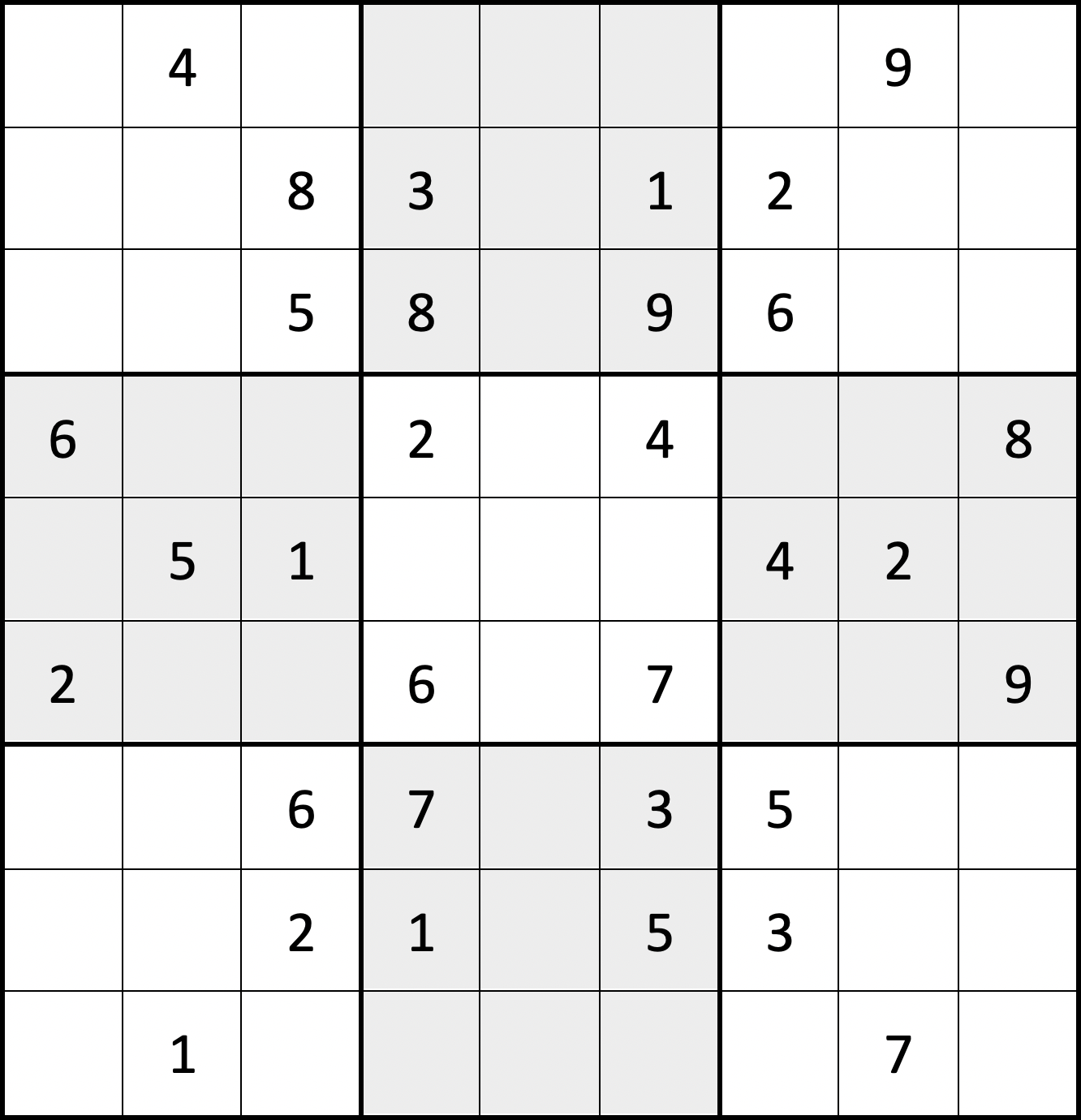
(a) Sudoku puzzle

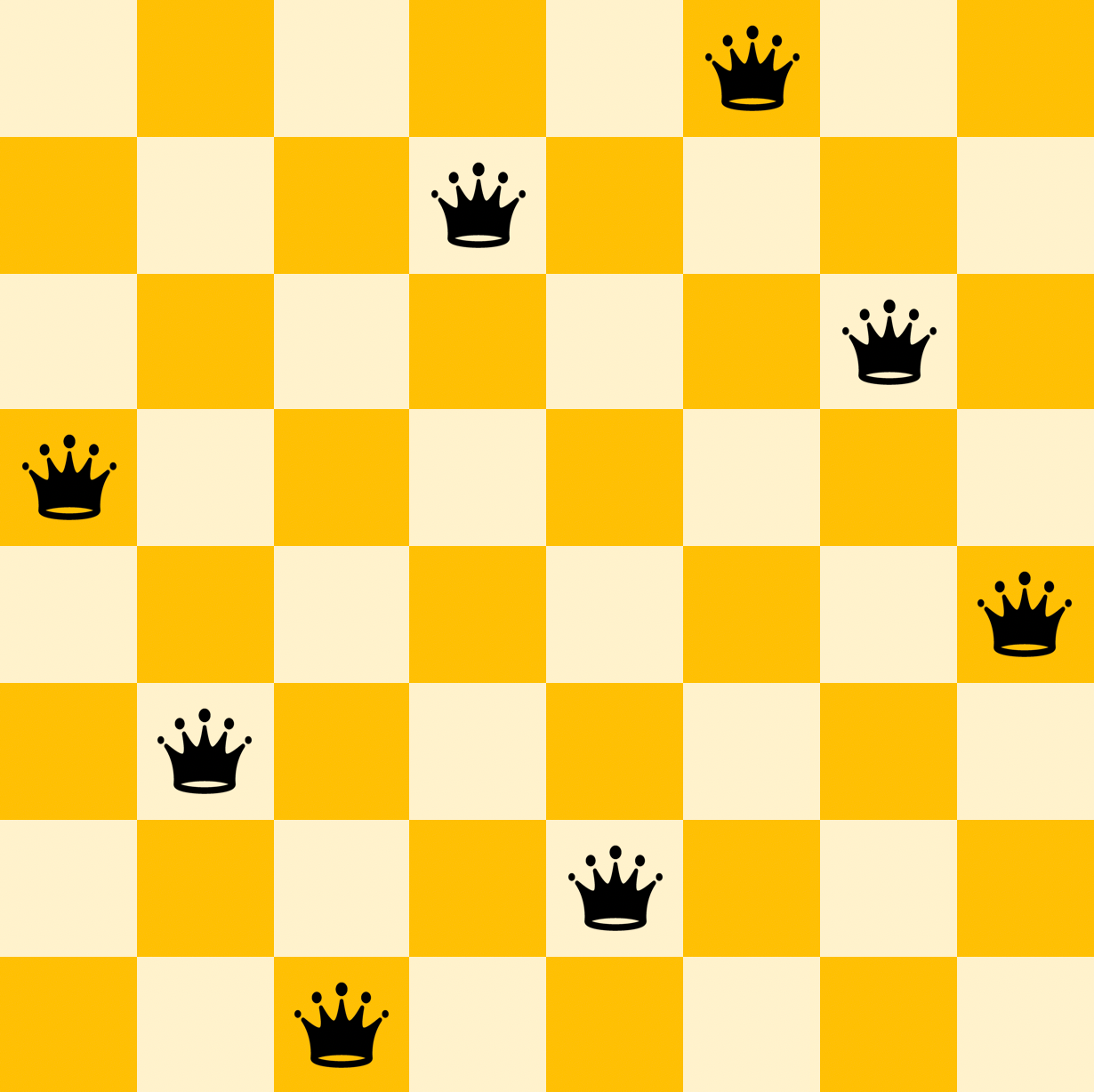
(b) Eight queens puzzle

Figure 3: Examples of Sudoku and eight queens. The goal of Sudoku is to complete the grid such that each row, column, and $3\times 3$ square contains all the digits from $1$ to $9$. The goal of eight queens is to place eight chess queens on an $8\times 8$ board such that no two queens share the same row/column/diagonal.

4.2.1 Sudoku puzzle

A standard Sudoku puzzle is shown in Figure 3 (a), which we generalize to grids of size $s\times s$ with the basic setting and rules:

• A partially complete $s\times s$ grid is provided.

• Each column, each row and each of the $s$ sub-grids of size $\sqrt{s}\times\sqrt{s}$ that compose the grid contain all of the digits from $1$ to $s$.

Based on the rules, we can easily formulate the Sudoku puzzle as feasibility problem. Here we consider the formulation proposed in [27], which formulates Sudoku as binary feasibility problem. We also refer to [2] for studies on Sudoku puzzle and Douglas–Rachford splitting method.

Each digit from $1$ to $s$ is lifted to the set $[0,1]^{s}$, making the full puzzle an $s\times s\times s$ binary cube. Figure 4 (a) shows a feasible row of the lifted problem represented as a binary $s\times s$ square. Equivalently, we can say that any digit from $1$ to $s$ is a permutation of unit vector $e=\{1,0,\ldots,0\}$. This leads to four Sudoku feasibility constraints:

• Each row of the cube, i.e. $C_{1}(:,j,k),\ j,k\in\{1,\ldots,s\}$, is the permutation of $e$; See Figure 4 (b).

• Each column of the cube, i.e. $C_{2}(i,:,k),\ i,k\in\{1,\ldots,s\}$, is the permutation of $e$; See Figure 4 (c).

• Each pillar of the cube, i.e. $C_{3}(i,j,:),\ i,j\in\{1,\ldots,s\}$, is the permutation of $e$; See Figure 4 (d).

• For each $k\in\{1,\ldots,s\}$, each of the $s$ sub-grids is the permutation of $e$, i.e. $C_{4}(\sqrt{s}(i-1)+1:\sqrt{s}i,\sqrt{s}(j-1)+1:\sqrt{s}j,k),\ i,j\in\{1,\ldots,\sqrt{s}\}$; See Figure 4 (e).

The partially completed grid forms the last constraint set

• $C_{5}$ is the constraint of the provided numbers.

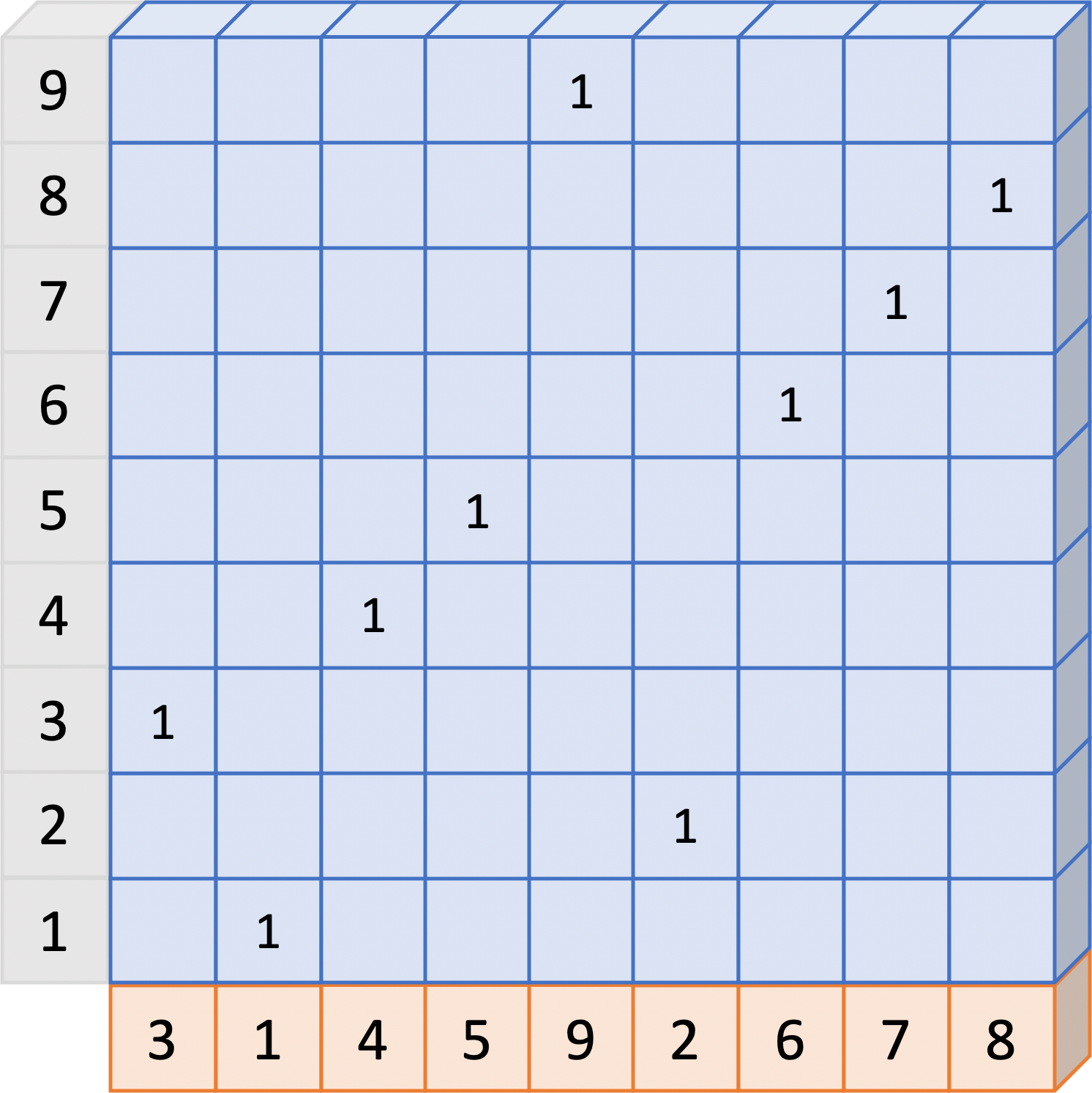
(a) Lifted row

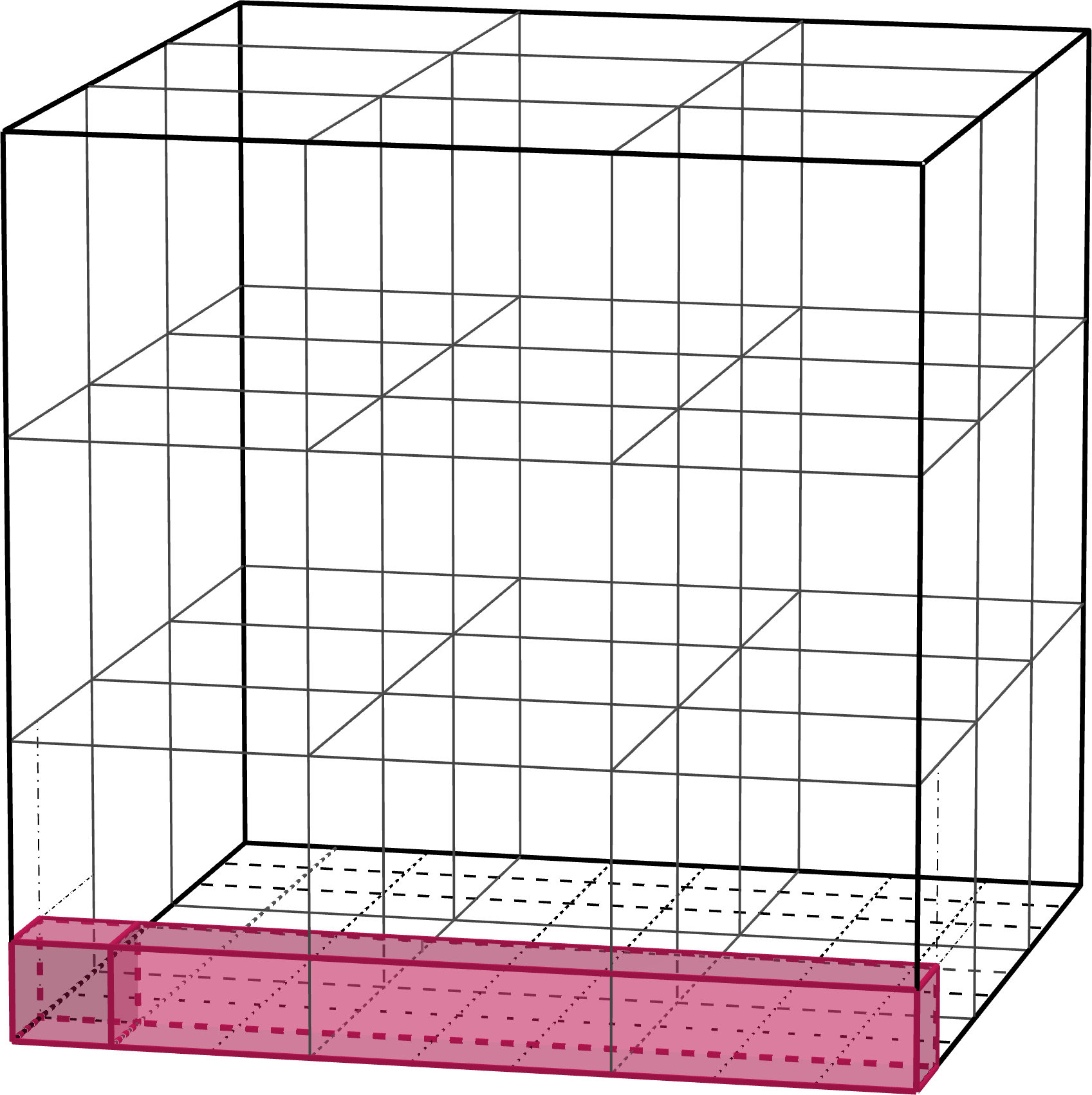
(b) $C_{1}$

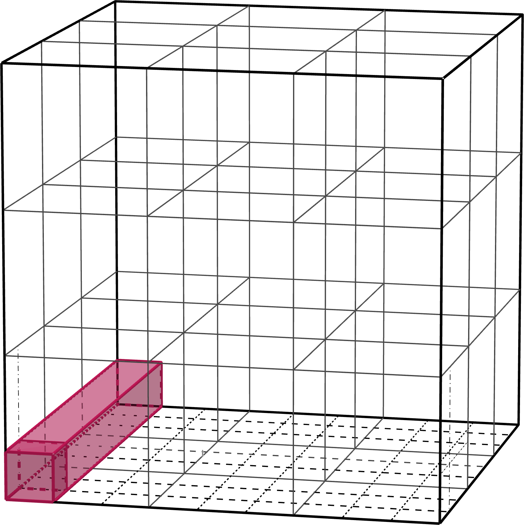
(c) $C_{2}$

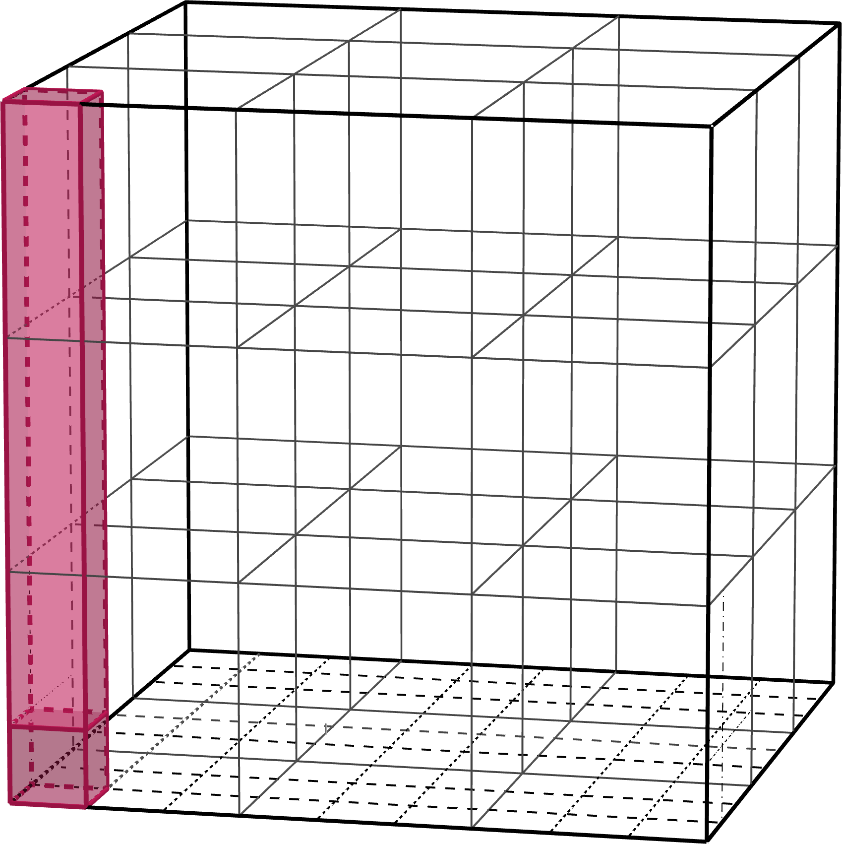
(d) $C_{3}$

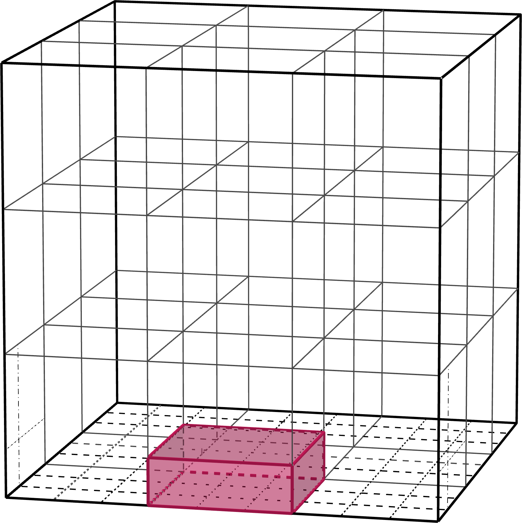
(e) $C_{4}$

Figure 4: Lifted Sudoku problem. (a) the lifted representation of a row of numbers. (b)-(e) show what is a lifted row/column/pillar/sub-grid respectively.

At this point, solving the Sudoku puzzle is equivalent to solve the following feasibility problem of the five constraint sets

$$\mathrm{find}\quad\,\,x\,\in\mathbb{R}^{s\times s\times s}\enskip\mathrm{s.t.}\enskip x\in C_{1}\cap C_{2}\cap C_{3}\cap C_{4}\cap C_{5}.$$ (4.7)

To obtain the product space formulation, let $\mathbfcal{H}=\underset{\textrm{$5$ times}}{\underbrace{\mathbb{R}^{s\times s\times s}\times\cdots\times\mathbb{R}^{s\times s\times s}}}$, $\mathbfcal{C}\stackrel{{\scriptstyle{\mathrm{def}}}}{{=}}C_{1}\times\dotsm\times C_{5}$, and $\mathbfcal{S}=\{\bm{x}=(x_{i})_{i}\in\mathbfcal{H}:x_{1}=\dotsm=x_{5}\}$.

Proposition 4.8 (Local convergence of DR).

For the Sudoku puzzle (4.7) and Douglas–Rachford splitting (3.9), suppose Assumptions A.1-A.4 hold. Then $\{\bm{u}_{k},x_{k},\bm{z}_{k}\}_{k\in\mathbb{N}}$ converges to $(\mathbfcal{K}(x^{\star}),x^{\star},\bm{z}^{\star})$ with $\bm{z}^{\star}\in\mathrm{Fix}(\mathscr{F}_{\mathrm{DR}})$ being a fixed point and $x^{\star}=\frac{1}{5}\sum_{i=1}^{5}z_{i}^{\star}$. If, moreover, for $i=1,\ldots,4$, $C_{i}$ is prox-regular at $x^{\star}$ for $x^{\star}-z_{i}^{\star}$ and the following non-degeneracy condition holds

$$x^{\star}-z_{i}^{\star}\in\mathrm{int}\big{(}{\mathscr{N}_{C_{i}}(x^{\star})}\big{)}.$$ (4.8)

Then for all $k$ large enough, there holds

• $u_{i,k}=x^{\star}$ for $i=1,\ldots,4$,

• ${|\kern-1.125pt|}\bm{z}_{k}-\bm{z}^{\star}{|\kern-1.125pt|}=O(\eta^{k})$ with $\eta=\frac{\sqrt{5}}{5}$.

• Denote $\bm{x}_{k+1}=\mathbfcal{K}(x_{k+1})$, from the updates of $\bm{x}_{k}$, we have that

  $$\bm{x}_{k+1}-\bm{x}^{\star}=\mathscr{P}_{\mathbfcal{S}}(\bm{z}_{k}-\bm{z}^{\star})$$

  with $\mathscr{P}_{\mathbfcal{S}}=\frac{1}{5}\mathbf{1}_{5\times 5}\otimes\mathrm{Id}_{s^{3}\times s^{3}}$, where $\mathbf{1}_{5\times 5}$ stands for matrix of all $1$ and $\otimes$ for Kronecker product.

  The separability of $\mathscr{P}_{\mathbfcal{C}}$ and the definition of projection operator lead to, for each $i=1,\ldots,5$

  $$u_{i,k+1} =\mathscr{P}_{C_{i}}(2x_{k+1}-z_{i,k})$$

  $$\quad\text{and}\quad u_{i,k+1}-u_{i}^{\star} =\mathscr{P}_{C_{i}}(2x_{k+1}-z_{i,k})-\mathscr{P}_{C_{i}}(2x^{\star}-z_{i}^{\star}).$$

  Under the non-degeneracy condition (4.8), apply the argument of Theorem 4.2 to obtain the finite convergence of $u_{i,k}$ for $i=1,\ldots,4$. For $C_{5}$, since its projection operator is linear, we have

  $$u_{5,k+1}-u_{5}^{\star} =\mathscr{P}_{C_{5}}(2x_{k+1}-z_{5,k})-\mathscr{P}_{C_{5}}(2x^{\star}-z_{5}^{\star})$$

  $$=2\mathscr{P}_{C_{5}}(x_{k+1}-x^{\star})-\mathscr{P}_{C_{5}}(z_{5,k}-z_{5}^{\star}).$$

  As a result, for $k$ large enough there holds

  $$\bm{u}_{k+1}-\bm{u}^{\star} =2\begin{bmatrix}\mathbf{0}_{4s^{3}\times 4s^{3}}&\\ &\mathscr{P}_{C_{5}}\end{bmatrix}\mathscr{P}_{\mathbfcal{S}}(\bm{z}_{k}-\bm{z}^{\star})-\begin{bmatrix}\mathbf{0}_{4s^{3}\times 4s^{3}}&\\ &\mathscr{P}_{C_{5}}\end{bmatrix}(\bm{z}_{k}-\bm{z}^{\star}).$$

  Let $\mathscr{P}_{\mathbfcal{C}}\stackrel{{\scriptstyle{\mathrm{def}}}}{{=}}\begin{bmatrix}\mathbf{0}_{4s^{3}\times 4s^{3}}&\\ &\mathscr{P}_{C_{5}}\end{bmatrix}$ and back to $\bm{z}_{k+1}-\bm{z}^{\star}$, we get

  $$\bm{z}_{k+1}-\bm{z}^{\star} =(\bm{z}_{k}-\bm{z}^{\star})+(\bm{u}_{k+1}-\bm{u}^{\star})-(\bm{x}_{k+1}-\bm{x}^{\star})$$

  $$=\big{(}{\mathbf{Id}+2\mathscr{P}_{\mathbfcal{C}}\mathscr{P}_{\mathbfcal{S}}-\mathscr{P}_{\mathbfcal{C}}-\mathscr{P}_{\mathbfcal{S}}}\big{)}(\bm{z}_{k}-\bm{z}^{\star}),$$

  Since $\mathscr{P}_{C_{5}}$ is the projection operator onto a subspace, so is $\mathscr{P}_{\mathbfcal{C}}$. As a result, the linear convergence rate is the cosine of the Friedrichs angle $\theta_{F}$ between the subspace of $\mathscr{P}_{\mathbfcal{C}}$ and that of $\mathscr{P}_{\mathbfcal{S}}$. We now need to analyze the singular values of $\mathscr{P}_{\mathbfcal{C}}\mathscr{P}_{\mathbfcal{S}}$, which essentially is the SVD of $\mathscr{P}_{C_{5}}\mathscr{P}_{S}$ where

  $$\mathscr{P}_{S}={{\frac{\raisebox{0.41669pt}{\footnotesize$1$}}{\raisebox{-1.24994pt}{\footnotesize$5$}}}}\mathbf{1}_{1\times 5}\otimes\mathrm{Id}_{s^{3}\times s^{3}}.$$

  We have

  • $\mathscr{P}_{C_{5}}$ is diagonal matrix with only $0$ and $1$.

  • $\mathscr{P}_{S}$ has a unique singular value which is $\frac{\sqrt{5}}{5}$.

  As a result, $\mathscr{P}_{C_{5}}\mathscr{P}_{S}$ has only two singular values which are $0$ and $\frac{\sqrt{5}}{5}$. Hence we conclude the proof. ∎

Next we present result for the damped Douglas–Rachford splitting (3.5).

Proposition 4.9 (Local convergence of dDR).

For the Sudoku puzzle (4.7) and the damped Douglas–Rachford splitting (3.10), suppose Assumptions A.1-A.3 hold and (3.10) is ran under the conditions of Theorem 3.1, then $(\bm{u}_{k},\bm{x}_{k},\bm{z}_{k})$ converges to $(\bm{x}^{\star},\bm{x}^{\star},\bm{z}^{\star})$ with $\bm{z}^{\star}$ being a fixed point and $\bm{x}^{\star}$ a stationary point of $\min_{\bm{x}}\left\{\mathrm{dist}^{2}(\bm{x},\mathbfcal{S})\,\,\mathrm{s.t.}\,\,\bm{x}\in\mathbfcal{C}\right\}$. If, moreover, the non-degeneracy condition (4.8) holds for $C_{1,\ldots,4}$, then for all $k$ large enough, it holds

• $u_{i,k}=x^{\star}$ for $i=1,\ldots,4$,

• ${|\kern-1.125pt|}\bm{z}_{k}-\bm{z}^{\star}{|\kern-1.125pt|}=O(\eta^{k})$ with $\eta=\frac{{2\gamma+5}+\sqrt{25-16\gamma^{2}}}{10(1+\gamma)}$.

• From the updates of $\bm{x}_{k+1}$, we have that

  $$\bm{x}_{k+1}-\bm{x}^{\star} ={{\frac{\raisebox{0.41669pt}{\footnotesize$1$}}{\raisebox{-1.24994pt}{\footnotesize$1+\gamma$}}}}\big{(}{\bm{z}_{k}+\gamma\mathscr{P}_{\mathbfcal{S}}(\bm{z}_{k})}\big{)}-{{\frac{\raisebox{0.41669pt}{\footnotesize$1$}}{\raisebox{-1.24994pt}{\footnotesize$1+\gamma$}}}}\big{(}{\bm{z}^{\star}+\gamma\mathscr{P}_{bcS}(\bm{z}^{\star})}\big{)}$$

  $$={{\frac{\raisebox{0.41669pt}{\footnotesize$1$}}{\raisebox{-1.24994pt}{\footnotesize$1+\gamma$}}}}(\bm{z}_{k}-\bm{z}^{\star})+{{\frac{\raisebox{0.41669pt}{\footnotesize$\gamma$}}{\raisebox{-1.24994pt}{\footnotesize$1+\gamma$}}}}\mathscr{P}_{\mathbfcal{S}}(\bm{z}_{k}-\bm{z}^{\star})$$

  with $\mathscr{P}_{\mathbfcal{S}}={{\frac{\raisebox{0.29167pt}{\footnotesize$1$}}{\raisebox{-0.87495pt}{\footnotesize$5$}}}}\mathbf{1}_{5\times 5}\otimes\mathrm{Id}_{s^{3}\times s^{3}}$. For $\bm{u}_{k}$, the finite termination of $u_{i,k},\,i=1,\ldots,4$ follows from the proof of Proposition 4.8. For $C_{5}$, again we have

  $$u_{5,k+1}-u_{5}^{\star}=2\mathscr{P}_{C_{5}}(x_{5,k+1}-x_{5}^{\star})-\mathscr{P}_{C_{5}}(z_{5,k}-z_{5}^{\star}).$$

  Let $\mathscr{P}_{\mathbfcal{C}}\stackrel{{\scriptstyle{\mathrm{def}}}}{{=}}\begin{bmatrix}\mathbf{0}_{4s^{3}\times 4s^{3}}&\\ &\mathscr{P}_{C_{5}}\end{bmatrix}$, then

  $$\bm{u}_{k+1}-\bm{u}^{\star} =2\mathscr{P}_{\mathbfcal{C}}(\bm{x}_{k+1}-\bm{x}^{\star})-\mathscr{P}_{\mathbfcal{C}}(\bm{z}_{k}-\bm{z}^{\star})$$

  $$={{\frac{\raisebox{0.41669pt}{\footnotesize$2$}}{\raisebox{-1.24994pt}{\footnotesize$1+\gamma$}}}}\mathscr{P}_{\mathbfcal{C}}(\bm{z}_{k}-\bm{z}^{\star})+{{\frac{\raisebox{0.41669pt}{\footnotesize$2\gamma$}}{\raisebox{-1.24994pt}{\footnotesize$1+\gamma$}}}}\mathscr{P}_{\mathbfcal{C}}\mathscr{P}_{\mathbfcal{S}}(\bm{z}_{k}-\bm{z}^{\star})-\mathscr{P}_{\mathbfcal{C}}(\bm{z}_{k}-\bm{z}^{\star})$$

  $$={{\frac{\raisebox{0.41669pt}{\footnotesize$1-\gamma$}}{\raisebox{-1.24994pt}{\footnotesize$1+\gamma$}}}}\mathscr{P}_{\mathbfcal{C}}(\bm{z}_{k}-\bm{z}^{\star})+{{\frac{\raisebox{0.41669pt}{\footnotesize$2\gamma$}}{\raisebox{-1.24994pt}{\footnotesize$1+\gamma$}}}}\mathscr{P}_{\mathbfcal{C}}\mathscr{P}_{\mathbfcal{S}}(\bm{z}_{k}-\bm{z}^{\star}).$$

  Back to $\bm{z}_{k+1}-\bm{z}^{\star}$, we get

  $$\bm{z}_{k+1}-\bm{z}^{\star} =(\bm{z}_{k}-\bm{z}^{\star})+(\bm{u}_{k+1}-\bm{u}^{\star})-(\bm{x}_{k+1}-\bm{x}^{\star})$$

  $$=(\bm{z}_{k}-\bm{z}^{\star})+{{\frac{\raisebox{0.41669pt}{\footnotesize$1-\gamma$}}{\raisebox{-1.24994pt}{\footnotesize$1+\gamma$}}}}\mathscr{P}_{\mathbfcal{C}}(\bm{z}_{k}-\bm{z}^{\star})+{{\frac{\raisebox{0.41669pt}{\footnotesize$2\gamma$}}{\raisebox{-1.24994pt}{\footnotesize$1+\gamma$}}}}\mathscr{P}_{\mathbfcal{C}}\mathscr{P}_{\mathbfcal{S}}(\bm{z}_{k}-\bm{z}^{\star})$$

  $$\qquad-{{\frac{\raisebox{0.41669pt}{\footnotesize$1$}}{\raisebox{-1.24994pt}{\footnotesize$1+\gamma$}}}}(\bm{z}_{k}-\bm{z}^{\star})-{{\frac{\raisebox{0.41669pt}{\footnotesize$\gamma$}}{\raisebox{-1.24994pt}{\footnotesize$1+\gamma$}}}}\mathscr{P}_{\mathbfcal{S}}(\bm{z}_{k}-\bm{z}^{\star})$$

  $$={{\frac{\raisebox{0.41669pt}{\footnotesize$1$}}{\raisebox{-1.24994pt}{\footnotesize$1+\gamma$}}}}\big{(}{{\gamma}\mathbf{Id}+{2\gamma}\mathscr{P}_{\mathbfcal{C}}\mathscr{P}_{\mathbfcal{S}}+(1-\gamma)\mathscr{P}_{\mathbfcal{C}}-{\gamma}\mathscr{P}_{\mathbfcal{S}}}\big{)}(\bm{z}_{k}-\bm{z}^{\star})$$

  $$={{\frac{\raisebox{0.41669pt}{\footnotesize$1$}}{\raisebox{-1.24994pt}{\footnotesize$1+\gamma$}}}}\big{(}{\gamma(\mathbf{Id}+2\mathscr{P}_{\mathbfcal{C}}\mathscr{P}_{\mathbfcal{S}}-\mathscr{P}_{\mathbfcal{C}}-\mathscr{P}_{\mathbfcal{S}})+\mathscr{P}_{\mathbfcal{C}}}\big{)}(\bm{z}_{k}-\bm{z}^{\star}).$$

  Denote $M_{\gamma}=\frac{1}{1+\gamma}(\gamma(\mathbf{Id}+2\mathscr{P}_{\mathbfcal{C}}\mathscr{P}_{\mathbfcal{S}}-\mathscr{P}_{\mathbfcal{C}}-\mathscr{P}_{\mathbfcal{S}})+\mathscr{P}_{\mathbfcal{C}})$. Let $p,q$ be the rank of $\mathscr{P}_{\mathbfcal{C}}$ and $\mathscr{P}_{\mathbfcal{S}}$ respectively, also assume $p\leq q$ (For the case $p\geq q$, similar result can be obtained). Based on [5], there exists an orthogonal matrix $U$ such that

  $$\mathscr{P}_{\mathbfcal{C}}=U\left[\begin{array}[]{cc|cc}\mathrm{Id}_{p}&0&0&0\\ 0&0_{p}&0&0\\ \hline\cr 0&0&0_{q-p}&0\\ 0&0&0&0_{n-p-q}\end{array}\right]U^{*}\\ \quad\text{and}\quad\mathscr{P}_{\mathbfcal{S}}=U\left[\begin{array}[]{cc|cc}\alpha^{2}&\alpha\beta&0&0\\ \alpha\beta&\beta^{2}&0&0\\ \hline\cr 0&0&\mathrm{Id}_{q-p}&0\\ 0&0&0&0_{n-p-q}\end{array}\right]U^{*},$$

  where $\alpha=\mathrm{diag}(\cos(\theta_{1}),\ldots,\cos(\theta_{p}))$ and $\beta=\mathrm{diag}(\sin(\theta_{1}),\ldots,\sin(\theta_{p}))$ with $\theta_{i,i=1,..p}$ being the principal angles between the subspaces of $\mathscr{P}_{\mathbfcal{C}}$ and $\mathscr{P}_{\mathbfcal{S}}$. Consequently,

  $$\mathbf{Id}+2\mathscr{P}_{\mathbfcal{C}}\mathscr{P}_{\mathbfcal{S}}-\mathscr{P}_{\mathbfcal{C}}-\mathscr{P}_{\mathbfcal{S}}=U\left[\begin{array}[]{cc|cc}\alpha^{2}&\alpha\beta&0&0\\ -\alpha\beta&\alpha^{2}&0&0\\ \hline\cr 0&0&0_{q-p}&0\\ 0&0&0&\mathrm{Id}_{n-p-q}\end{array}\right]U^{*}.$$

  Therefore, we have

  $$M_{\gamma}={{\frac{\raisebox{0.41669pt}{\footnotesize$1$}}{\raisebox{-1.24994pt}{\footnotesize$1+\gamma$}}}}U\left[\begin{array}[]{cc|cc}\gamma\alpha^{2}+\mathrm{Id}_{p}&\gamma\alpha\beta&0&0\\ -\gamma\alpha\beta&\gamma\alpha^{2}&0&0\\ \hline\cr 0&0&0_{q-p}&0\\ 0&0&0&\gamma\mathrm{Id}_{n-p-q}\end{array}\right]U^{*}$$

  Clearly, $0$ and $\frac{\gamma}{1+\gamma}$ are two eigenvalues of the matrix. For the top left block of the above matrix, as it is block diagonal, we have the following characteristic polynomial

  $$0=\prod_{i=1}^{p}{\big{(}}{\big{(}{\tfrac{\gamma\alpha_{i}^{2}+1}{1+\gamma}-\lambda}\big{)}\big{(}{\tfrac{\gamma\alpha_{i}^{2}}{1+\gamma}-\lambda}\big{)}+\tfrac{\gamma^{2}\alpha_{i}^{2}\beta_{i}^{2}}{(1+\gamma)^{2}}}{\big{)}}.$$

  Solving the quadratic equation for each $i$ we get

  $$\lambda_{i}={{\frac{\raisebox{1.24994pt}{\small${2\gamma\alpha_{i}^{2}+1}\pm\sqrt{1-4\gamma^{2}\alpha_{i}^{2}\beta_{i}^{2}}$}}{\raisebox{-2.08333pt}{\small$2(1+\gamma)$}}}}.$$

  As in the proof of Proposition 4.8, we have that $\alpha_{i}=\frac{\sqrt{5}}{5}$ for all $i=1,\ldots,p$, therefore $M_{\gamma}$ has only $4$ distinct eigenvalues which are

  $$0,\quad{{\frac{\raisebox{0.41669pt}{\footnotesize${2\gamma+5}-\sqrt{25-16\gamma^{2}}$}}{\raisebox{-1.24994pt}{\footnotesize$10(1+\gamma)$}}}},\quad{{\frac{\raisebox{0.41669pt}{\footnotesize$\gamma$}}{\raisebox{-1.24994pt}{\footnotesize$1+\gamma$}}}}\quad\text{and}\quad{{\frac{\raisebox{0.41669pt}{\footnotesize${2\gamma+5}+\sqrt{25-16\gamma^{2}}$}}{\raisebox{-1.24994pt}{\footnotesize$10(1+\gamma)$}}}}.$$

  We also have

  $${{\frac{\raisebox{0.41669pt}{\footnotesize$\gamma$}}{\raisebox{-1.24994pt}{\footnotesize$1+\gamma$}}}}\leq{{\frac{\raisebox{0.41669pt}{\footnotesize${2\gamma+5}+\sqrt{25-16\gamma^{2}}$}}{\raisebox{-1.24994pt}{\footnotesize$10(1+\gamma)$}}}} :\gamma\in]0,1],$$

  $${{\frac{\raisebox{0.41669pt}{\footnotesize$\gamma$}}{\raisebox{-1.24994pt}{\footnotesize$1+\gamma$}}}}\geq{\lvert}{{\frac{\raisebox{0.41669pt}{\footnotesize${2\gamma+5}+\sqrt{25-16\gamma^{2}}$}}{\raisebox{-1.24994pt}{\footnotesize$10(1+\gamma)$}}}}{\rvert} :\gamma\in]1,+\infty[$$

  Next we focus on $\gamma\in]0,1]$ and show $\eta=\frac{{2\gamma+5}+\sqrt{25-16\gamma^{2}}}{10(1+\gamma)}$ is the convergence rate, to this end, we need to show $\eta$ is semi-simple. Let $M_{p}=\begin{bmatrix}\gamma\alpha^{2}+\mathrm{Id}_{p}&\gamma\alpha\beta\\ -\gamma\alpha\beta&\gamma\alpha^{2}\end{bmatrix}$, since $\alpha=\frac{\sqrt{5}}{5}$ is a $p$’th order root, we can simplify $M_{p}$ as:

  $$M_{p}={{\frac{\raisebox{0.41669pt}{\footnotesize$1$}}{\raisebox{-1.24994pt}{\footnotesize$5$}}}}\begin{bmatrix}(\gamma+5)\mathrm{Id}_{p}&{2\gamma}\mathrm{Id}_{p}\\ -{2\gamma}\mathrm{Id}_{p}&{\gamma}\mathrm{Id}_{p}\end{bmatrix}$$

  As a result, we have

  $$\mathrm{rank}(M_{p}-\eta\mathrm{Id}_{2p}) =\mathrm{rank}\left({\small\begin{bmatrix}(\gamma+5-5\eta)\mathrm{Id}_{p}&{2\gamma}\mathrm{Id}_{p}\\ -{2\gamma}\mathrm{Id}_{p}&(\gamma-5\eta)\mathrm{Id}_{p}\end{bmatrix}}\right)=p,\quad\text{and}\quad$$

  $$\mathrm{rank}\big{(}{(M_{p}-\eta\mathrm{Id}_{2p})^{2}}\big{)} =\mathrm{rank}\left({\small\begin{bmatrix}((\gamma+5-5\eta)^{2}-4\gamma^{2})\mathrm{Id}_{p}&{2\gamma}(\gamma+5-10\eta)\mathrm{Id}_{p}\\ -{2\gamma}(\gamma+5-10\eta)\mathrm{Id}_{p}&((\gamma-5\eta)^{2}-4\gamma^{2})\mathrm{Id}_{p}\end{bmatrix}}\right)=p,$$

  which means $\eta$ is semi-simple by Definition 2.6, and we conclude the linear rate of convergence. ∎

Remark 4.10.

The proofs of the two propositions above is dimension independent, which means the results hold true for all puzzle sizes of perfect squares $s$ with $s\geq 4$. See Section 5 for numerical illustrations.

4.3 $s$-queens puzzle

The rule of eight queens puzzle is rather simple: placing eight chess queens on an $8\times 8$ chessboard so that no two queens threaten each other. The size of puzzle can be generalized to any size $s\times s$ with $s\geq 4$, while there is no solution for $s=2,3$ and a trivial solution for $s=1$ which is obvious.

We follow the setting of [27]. On the chessboard, as there are four directions (horizontal, vertical and two diagonal directions) for the queen to move, we have four constraint sets for the problem:

• $C_{1}$: each row has only one queen.

• $C_{2}$: each column has only one queen.

• $C_{3}$: each diagonal direction southeast-northwest, there is at most one queen.

• $C_{4}$: each diagonal direction southwest-northeast, there is at most one queen.

Now we can formulate the $s$-queens puzzle as a feasibility problem of four sets

$$\mathrm{find}\quad\,\,x\,\in\mathbb{R}^{s\times s}\enskip\mathrm{s.t.}\enskip x\in C_{1}\cap C_{2}\cap C_{3}\cap C_{4}.$$ (4.9)

Since all the sets above are binary, so is the set $\mathbfcal{C}\stackrel{{\scriptstyle{\mathrm{def}}}}{{=}}C_{1}\times\dotsm\times C_{4}$, as a result finite convergence can be obtained under the conditions of Theorems 4.2 and 4.5, for the standard Douglas–Rachford and the damped one, respectively.

5 Numerical results

We now provide numerical results on Sudoku and $s$-queens puzzles to support our theoretical findings. Before analyzing the convergence rates, we first compare the performance of the standard Douglas–Rachford splitting method (3.2) and the damped one (3.5), on how successful are they when applied to solve these two puzzles. i.e. how often each method finds a feasible point.

The comparison is shown in Table 1. For (3.5), two choices of $\gamma$ are considered: $\gamma=\frac{1}{5}\in]0,\sqrt{3/2}-1[$ suggested by Lemma 3.1 and $\gamma=99$ with online tracking rule suggested in [19, Remark 4]. For both methods, the iteration is terminated if either a stopping criterion is met or $10^{4}$ steps of iteration are reached, then we verify the output. Also, a minimal $100$ number of iteration is set. For a given puzzle, each method is repeated $10^{3}$ times with different initialization for each running.

For Sudoku, the size of both puzzles are $9\times 9$: “Puzzle 1” is provided with $37$ digits, hence is easy; “Puzzle 2” has $22$ given digits and is more difficult than “Puzzle 1”

• The standard DR solves both puzzles with $100\%$ success rate, while dDR with $\gamma=\frac{1}{5}$ fails all tests. dDR with $\gamma=99$ succeeds on “Puzzle 1” and the rate drops to about $88\%$ for “Puzzle 2”.

• In terms of number of iteration, sDR needs much less number of iterations compared to those of dDR with $\gamma=99$.

For $s$-queens puzzle, two different sizes are considered: $s=8$ for “Puzzle 1” and $s=16$ for “Puzzle 2”.

• Similar to Sudoku, dDR with $\gamma=\frac{1}{5}$ fails all tests. This time, between sDR and dDR with $\gamma=99$, neither achieves $100\%$ success rate with dDR being better than sDR.

• In terms of number of iteration, same as Sudoku case, sDR is better.

The above observation, in particular the failure of dDR with $\gamma=\frac{1}{5}$, is in contrast to Example 3.2. One possible reason leads to the failure of dDR with $\gamma=\frac{1}{5}$, is that the set $C$ is finite and dDR can not escape bad local stationary point with small value of $\gamma$.

Table 1: Comparison of success rate of standard DR and damped DR for solving Sudoku and $s$-queens puzzles over 1,000 random initializations.

		Puzzle 1			Puzzle 2
		sDR	dDR $\gamma=\frac{1}{5}$	dDR $\gamma=99$	sDR	dDR $\gamma=\frac{1}{5}$	dDR $\gamma=99$
Sudoku	success rate	100%	0	100%	100%	0	89.7%
	avg. # of itr.	114	184	2710	408	184	5409
$s$-queens	success rate	94.8%	0	98.0%	90.2%	0	92.2%
	avg. # of itr.	653	100	2812	1286	100	3618

5.1 Sudoku puzzle

We consider three different puzzle sizes for Sudoku to verify out results: $4$, $9$ and $16$, which are shown in Figure 5 (a)-(c). In each size, we have $4$, $32$, and $128$ coefficients provided respectively. The convergence behavior of standard Douglas–Rachford splitting method can be seen in the second and third rows of Figure 5, from which we observe that for all puzzles,

• Finite termination of $u_{i,k},i=1,\ldots,4$: in the second row of Figure 5, we provide the $\ell_{0}$ pseudo-norms of ${|\kern-1.125pt|}u_{i,k}-u_{i}^{\star}{|\kern-1.125pt|}_{0},i=1,\ldots,4$ to show the mismatch between $u_{i,k}$ and $u_{i}^{\star}$. We observed that, for each $i\in\{1,2,3,4\}$, ${|\kern-1.125pt|}u_{i,k}-u_{i}^{\star}{|\kern-1.125pt|}_{0}$ reaches $0$ in finite steps, which means the finite termination.

• Local linear convergence In the last row of Figure 5, we provide the convergence behaviors of ${|\kern-1.125pt|}\bm{u}_{k}-\bm{u}^{\star}{|\kern-1.125pt|}$ (which actually reduces to ${|\kern-1.125pt|}u_{5,k}-u_{5}^{\star}{|\kern-1.125pt|}$), ${|\kern-1.125pt|}x_{k}-x^{\star}{|\kern-1.125pt|}$ and ${|\kern-1.125pt|}\bm{z}_{k}-\bm{z}^{\star}{|\kern-1.125pt|}$. Take ${|\kern-1.125pt|}\bm{z}_{k}-\bm{z}^{\star}{|\kern-1.125pt|}$ for example, its convergence has two different regimes: sub-linear rate from the beginning, and linear rate locally. The magenta dashed line is our theoretical estimation of the linear convergence rate and the slope of the line is $\frac{\sqrt{5}}{5}$.

For all three different puzzle sizes, the local linear convergence rate is $\frac{\sqrt{5}}{5}\approx 0.45$, which confirms that the rate is independent of puzzle size.

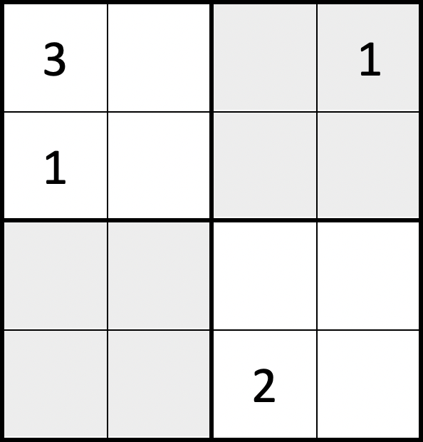
(a) Size $4\times 4$

(b) Size $9\times 9$

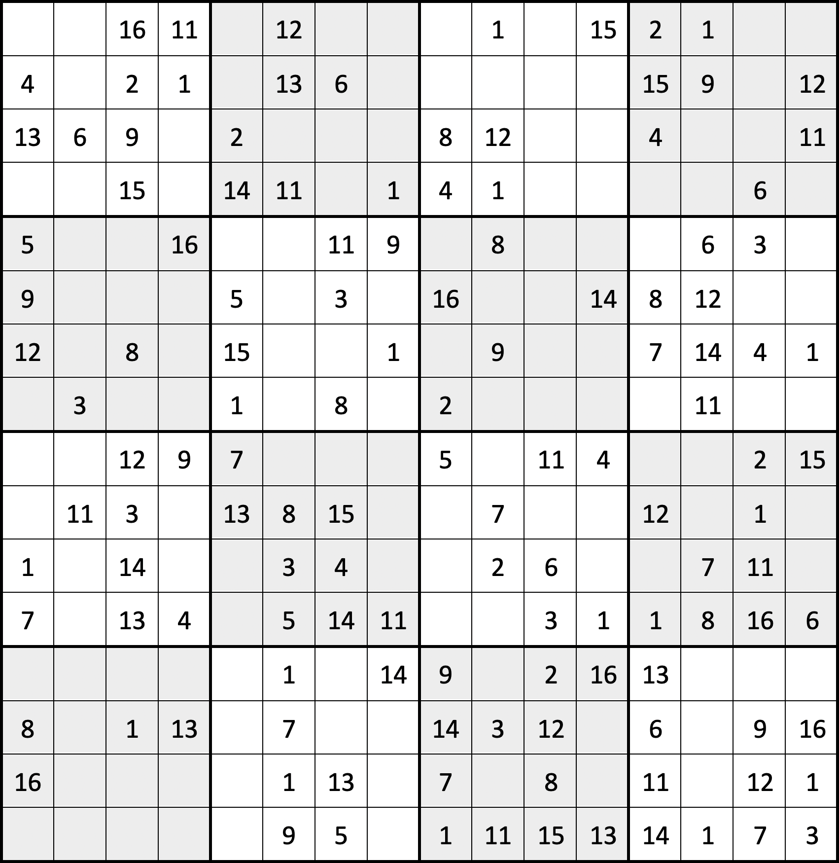
(c) Size $16\times 16$

(d) Size $4$: convergence of $u_{i,k}$

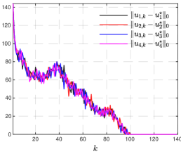
(e) Size $9$: convergence of $u_{i,k}$

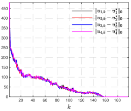
(f) Size $16$: convergence of $u_{i,k}$

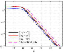
(g) Size $4$: convergence of $(\bm{u}_{k},x_{k},\bm{z}_{k})$

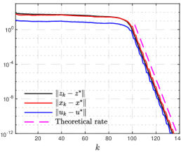
(h) Size $9$: convergence of $(\bm{u}_{k},x_{k},\bm{z}_{k})$

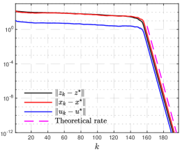
(i) Size $16$: convergence of $(\bm{u}_{k},x_{k},\bm{z}_{k})$

Figure 5: Different sizes of Sudoku puzzles and convergence observations.

5.2 $s$-queens puzzle

For the $s$-queens puzzle, we also consider three different puzzle sizes: $s=8,16$ and $25$, which are shown in Figure 6 (a)-(c). The convergence behaviors of the Douglas–Rachford splitting method are shown in the second row of Figure 6. Since all the constraint sets are binary, we observe finite convergence for the algorithm which complies with our theoretical results.

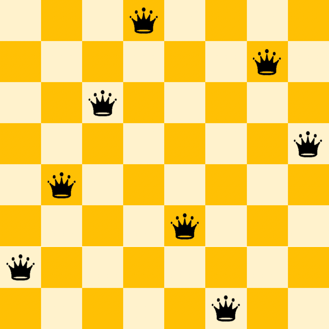
(a) Size 8

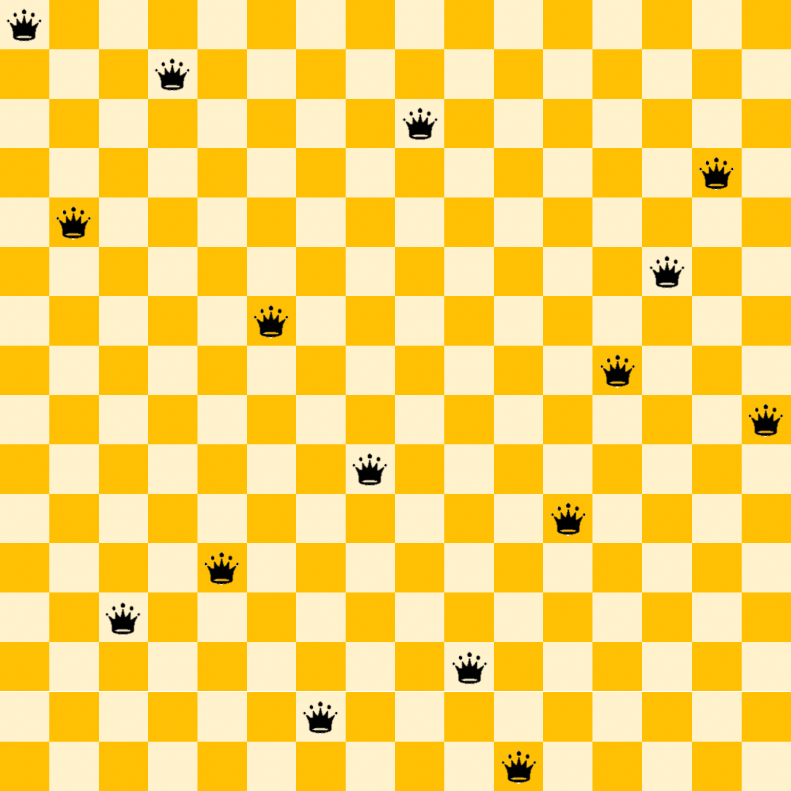
(b) Size 16

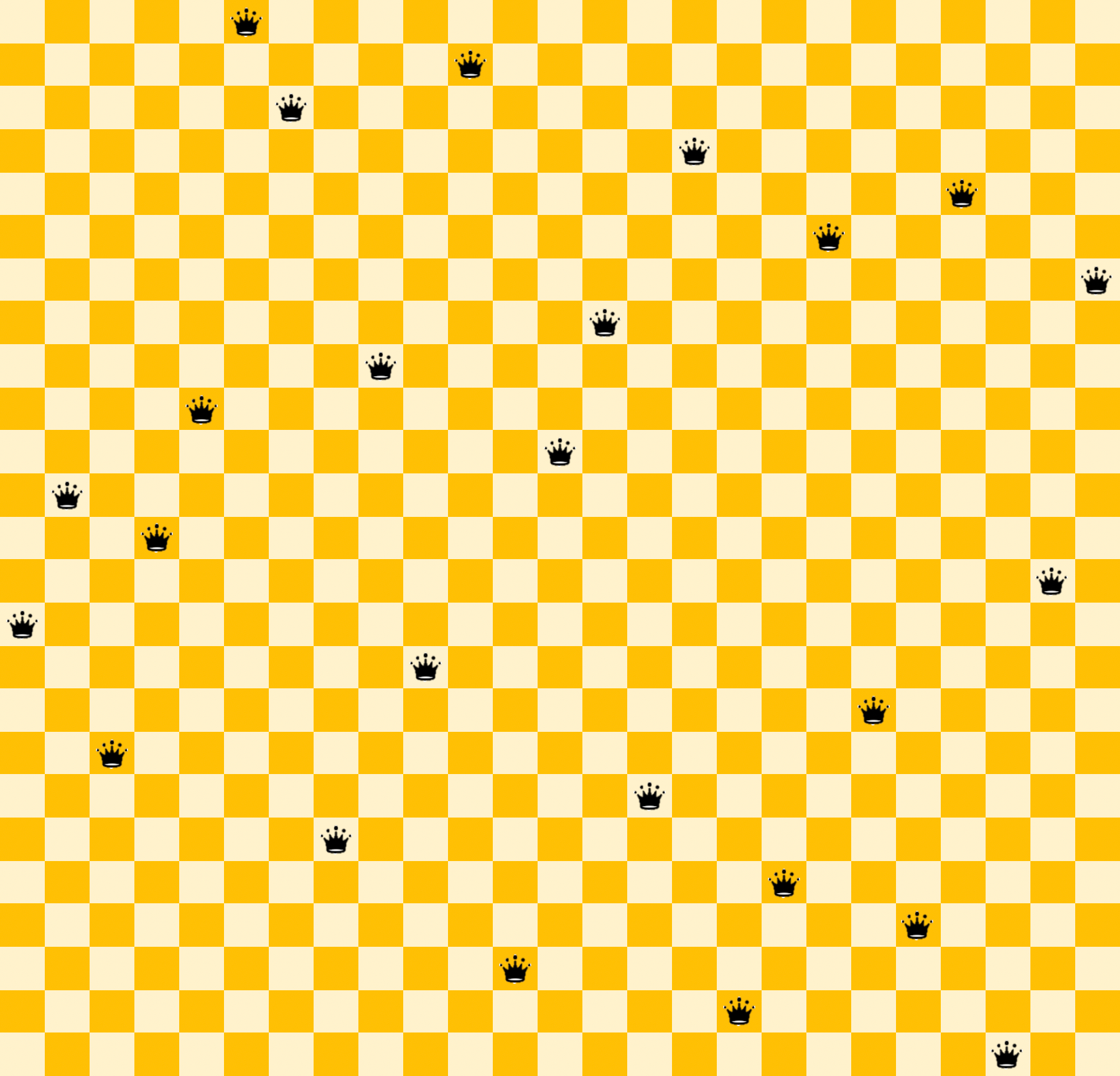
(c) Size 25

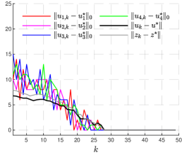
(d) Size 8

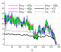
(e) Size 16

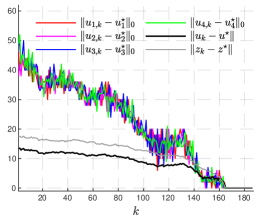
(f) Size 25

Figure 6: Different sizes of queens puzzles and convergence observations.

5.3 The damped Douglas–Rachford splitting

We conclude our numerical experiments by showing the local linear convergence the damped Douglas–Rachford splitting method with $\gamma=99$. The results on Sudoku puzzle of size $9\times 9$ and eight queens puzzle of size $8\times 8$ are shown below in Figure 7. For both plots, the magenta line is our theoretical estimation of the local linear rate:

• For Sudoku puzzle, the slope of the magenta line is $\frac{{2\gamma+5}+\sqrt{25-16\gamma^{2}}}{10(1+\gamma)}\approx 0.86$.

• For eight queens puzzle, the slope of the magenta line is $\frac{\gamma}{1+\gamma}\approx 0.17$.

Again, our theoretical estimations are tight. We omit the plots of dDR with $\gamma=99$ as they are very similar to those of Figure 7, except different rates of local linear convergence.

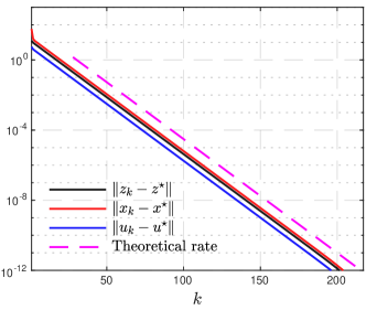
(a) Sudoku puzzle

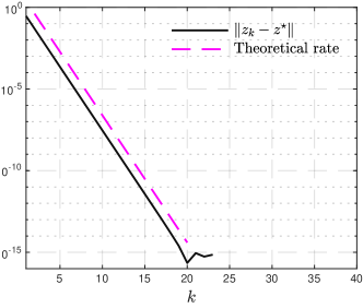
(b) Eight queens puzzle

Figure 7: Local linear convergence of the damped Douglas-Rachford for Sudoku puzzle and eight queens puzzle. Note again that convergence does not imply finding a solution to the feasibility problem.

6 Conclusions

In this paper, we studied local convergence properties of Douglas–Rachford splitting method when applied to solve non-convex feasibility problems. Under a proper non-degeneracy condition, both finite convergence and local linear convergence are proved for the standard Douglas–Rachford splitting and a damped version of the method. Understanding when the methods fail, especially for the damped Douglas–Rachford splitting, require further study on the property of the methods.

Acknowledgement

We would like to thank Guoyin Li for helpful discussions on the convergence of Douglas–Rachford splitting for non-convex optimization. J.L. was partly supported by Leverhulme trust, Newton trust and the EPSRC centre “EP/N014588/1”. R.T. acknowledges funding from EPSRC Grant No. “EP/L016516/1” for the Cambridge Centre for Analysis. Both authors were supported by the Cantab Capital Institute for Mathematics of Information.

References

- [1] F. J. A. Artacho and J. M. Borwein. Global convergence of a non-convex douglas–rachford iteration. Journal of Global Optimization, 57(3):753–769, 2013.
- [2] F. J. A. Artacho, J. M. Borwein, and M. K. Tam. Recent results on douglas–rachford methods for combinatorial optimization problems. Journal of Optimization Theory and Applications, 163(1):1–30, 2014.
- [3] F. J. A. Artacho, J. M. Borwein, and M. K. Tam. Global behavior of the douglas–rachford method for a nonconvex feasibility problem. Journal of Global Optimization, 65(2):309–327, 2016.
- [4] H. Attouch, J. Bolte, P. Redont, and A. Soubeyran. Proximal alternating minimization and projection methods for nonconvex problems: An approach based on the Kurdyka-Łojasiewicz inequality. Mathematics of Operations Research, 35(2):438–457, 2010.
- [5] H. H. Bauschke, J. Y. Bello Cruz, T. T. A. Nghia, H. M. Pha, and X. Wang. Optimal rates of linear convergence of relaxed alternating projections and generalized douglas-rachford methods for two subspaces. Numerical Algorithms, 73(1):33–76, 2016.
- [6] H. H. Bauschke and J. M. Borwein. On projection algorithms for solving convex feasibility problems. SIAM review, 38(3):367–426, 1996.
- [7] H. H. Bauschke and M. N. Dao. On the finite convergence of the douglas–rachford algorithm for solving (not necessarily convex) feasibility problems in euclidean spaces. SIAM Journal on Optimization, 27(1):507–537, 2017.
- [8] H. H. Bauschke and D. Noll. On the local convergence of the douglas–rachford algorithm. Archiv der Mathematik, 102(6):589–600, 2014.
- [9] Heinz H Bauschke, JY Bello Cruz, Tran TA Nghia, Hung M Pha, and Xianfu Wang. Optimal rates of linear convergence of relaxed alternating projections and generalized douglas-rachford methods for two subspaces. Numerical Algorithms, 73(1):33–76, 2016.
- [10] Heinz H Bauschke, Minh N Dao, Dominikus Noll, and Hung M Phan. On slater’s condition and finite convergence of the douglas–rachford algorithm for solving convex feasibility problems in euclidean spaces. Journal of Global Optimization, 65(2):329–349, 2016.
- [11] L. M. Bregman. The method of successive projection for finding a common point of convex sets. Sov. Math. Dok., 162(3):688–692, 1965.
- [12] A. Cegielski and A. Suchocka. Relaxed alternating projection methods. SIAM Journal on Optimization, 19(3):1093–1106, 2008.
- [13] P. L. Combettes and J. C. Pesquet. Proximal splitting methods in signal processing. In Fixed-Point Algorithms for Inverse Problems in Science and Engineering, pages 185–212. Springer, 2011.
- [14] J. Douglas and H. H. Rachford. On the numerical solution of heat conduction problems in two and three space variables. Transactions of the American mathematical Society, 82(2):421–439, 1956.
- [15] R. Hesse and D. R. Luke. Nonconvex notions of regularity and convergence of fundamental algorithms for feasibility problems. SIAM Journal on Optimization, 23(4):2397–2419, 2013.
- [16] R. Hesse, D. R. Luke, and P. Neumann. Projection methods for sparse affine feasibility: Results and counterexamples. Technical report, 2013.
- [17] R. Hesse, D. R. Luke, and P. Neumann. Alternating projections and douglas-rachford for sparse affine feasibility. IEEE Transactions on Signal Processing, 62(18):4868–4881, 2014.
- [18] A. S. Lewis. Active sets, nonsmoothness, and sensitivity. SIAM Journal on Optimization, 13(3):702–725, 2003.
- [19] G. Li and T. Kei. Pong. Douglas–rachford splitting for nonconvex optimization with application to nonconvex feasibility problems. Mathematical programming, 159(1-2):371–401, 2016.
- [20] J. Liang, J. Fadili, and G. Peyré. Local convergence properties of douglas–rachford and alternating direction method of multipliers. Journal of Optimization Theory and Applications, 172(3):874–913, 2017.
- [21] P. L. Lions and B. Mercier. Splitting algorithms for the sum of two nonlinear operators. SIAM Journal on Numerical Analysis, 16(6):964–979, 1979.
- [22] D. R. Luke. Relaxed averaged alternating reflections for diffraction imaging. Inverse problems, 21(1):37, 2004.
- [23] S.-Y. Matsushita and L. Xu. On the finite termination of the douglas-rachford method for the convex feasibility problem. Optimization, 65(11):2037–2047, 2016.
- [24] C. D. Meyer. Matrix analysis and applied linear algebra, volume 2. SIAM, 2000.
- [25] D. W. Peaceman and H. H. Rachford, Jr. The numerical solution of parabolic and elliptic differential equations. Journal of the Society for Industrial and Applied Mathematics, 3(1):28–41, 1955.
- [26] H. M. Phan. Linear convergence of the douglas–rachford method for two closed sets. Optimization, 65(2):369–385, 2016.
- [27] J. Schaad. Modeling the 8-queens problem and sudoku using an algorithm based on projections onto nonconvex sets. PhD thesis, University of British Columbia, 2010.
- [28] A. Themelis and P. Patrinos. Douglas–rachford splitting and admm for nonconvex optimization: Tight convergence results. SIAM Journal on Optimization, 30(1):149–181, 2020.
- [29] J von Neumann. Functional operators, vol. 2 (annals of mathematics studies, no. 22), princeton, nj, 1950. Reprinted from mimeographed lecture notes first distributed in, 1933.