Bayesian Inverse Reinforcement Learning for Collective Animal Movement

Abstract

Agent-based methods allow for defining simple rules that generate complex group behaviors. The governing rules of such models are typically set a priori and parameters are tuned from observed behavior trajectories. Instead of making simplifying assumptions across all anticipated scenarios, inverse reinforcement learning provides inference on the short-term (local) rules governing long term behavior policies by using properties of a Markov decision process. We use the computationally efficient linearly-solvable Markov decision process to learn the local rules governing collective movement for a simulation of the self propelled-particle (SPP) model and a data application for a captive guppy population. The estimation of the behavioral decision costs is done in a Bayesian framework with basis function smoothing. We recover the true costs in the SPP simulation and find the guppies value collective movement more than targeted movement toward shelter.

, and

1 Introduction

Understanding individual animal decision-making processes in social groups is challenging. Traditionally, agent-based models (ABMs) of individual interactions are used as building blocks for complex group dynamics (Vicsek et al., 1995; Couzin et al., 2002; Scharf et al., 2016; McDermott, Wikle and Millspaugh, 2017; Scharf et al., 2018). ABMs attempt to recreate what is observed in nature by defining a mechanistic model a priori. While the simple individual-based rules lead to complex group dynamics, ABMs suffer from preprogrammed behavior after reaching some equilibrium, challenges to incorporate interactions with habitat, and no notion of memory (Ried, Müller and Briegel, 2019). The goal of inverse modeling is to instead learn the underlying local rules from observations of sequential behavior decisions (Lee et al., 2017; Kangasrääsiö and Kaski, 2018; Yamaguchi et al., 2018).

Parameters of ABMs in practice need to be tuned or learned by supervised learning (Ried, Müller and Briegel, 2019; Wikle and Hooten, 2016; Hooten, Wikle and Schwob, 2020). A recent alternative to supervised learning is reinforcement learning (RL). RL is goal-oriented learning from continuous interaction between an agent and its environment (Sutton and Barto, 1998). That is, RL methods learn parameters controlling global behavior by trial and error experiments within the defined environment and local rules. The agents learn preferences by paying costs to (or receiving rewards from) the environment and choose optimal behavior by minimizing the cumulative expected future costs (also referred to as “costs-to-go”). Similar to difficulty in tuning ABMs, defining the cost function to produce desired long term behavior is challenging (Ng and Russell, 2000; Finn, Levine and Abbeel, 2016; Arora and Doshi, 2018).

In systems where observations of behavior trajectories can be collected, inverse reinforcement learning (IRL) methods aim to learn the state costs or costs-to-go that governed the observed agents’ decisions. Ng and Russell (2000) introduced the first IRL algorithms including dynamic programming, which solves a system of equations based on the state transition probabilities and a grid search method for exploring potential state costs that may have generated observed trajectory samples. As surveyed by Arora and Doshi (2018), many more methods have since been developed or adapted to address problems of meaningful size and non-identifiability of the costs. In fact, Ng and Russell (2000) showed in general there does not exist a unique solution to the state costs for systems with finite state space which requires subsequent modeling assumptions. The methods can be broadly categorized as maximum margin optimization (Ratliff, Bagnell and Zinkevich, 2006), entropy optimization (Ziebart et al., 2008), Bayesian IRL (Ramachandran and Amir, 2007; Choi and Kim, 2011; Jin et al., 2017; Sošić, Zoubir and Koeppl, 2017), and deep learning IRL (Wulfmeier, Ondruska and Posner, 2015), with the majority of the methods being applied to Markov decision processes (MDPs). The benefit of Bayesian frameworks to address the non-identifiability of costs in IRL is that they provide a distribution of costs that can generate the observed expert behavior and incorporate prior information to constrain state costs (Ramachandran and Amir, 2007).

Many of the aforementioned methods parameterize the likelihood by the immediate state costs, because the state cost function is a concise description of the task (Ng and Russell, 2000; Ramachandran and Amir, 2007). A computational challenge associated with parametrizing the likelihood by the costs is the necessity to solve the forward MDP each iteration as often the likelihood still involves calculating the state costs-to-go. An alternative class of MDP, the linearly-solvable MDP (LMDP) introduced by Todorov (2009), is linear in its solution for the optimal policy and thus, less computationally costly for forward modeling. The LMDP is defined by a set of passive dynamics that describe an agent’s state transitions in the absence of state costs or environmental feedback and then the optimal state transitions minimize costs-to-go. Moreover, IRL for LMDPs does not require the forward solution for each iteration as there is a linear relationship between the costs-to-go and immediate state costs. Therefore, inference about immediate state costs can be obtained by transformation of the estimated costs-to-go. As a special case, Dvijotham and Todorov (2010) showed that maximum entropy IRL is the solution to an LMDP with uniform passive dynamics. However, the maximum entropy IRL algorithms are parameterized by the state costs and require the computationally intensive step of solving the forward RL problem (Ziebart et al., 2008). Kohjima, Matsubayashi and Sawada (2017) proposed a Bayesian IRL method for learning state costs-to-go for LMDPs using variational approximation.

As argued by Ried, Müller and Briegel (2019), an MDP (or LMDP) for collective animal movement is a better model for the system than traditional self-propelled particle (SPP) models (Vicsek et al., 1995). The MDP incorporates the internal processes of an animal by modeling the behavior as perception (state space), planning (state values), and action (see Hooten, Scharf and Morales (2019) for related individual-level models). Furthermore, the behavior is governed by feedback from the environment (which includes other agents) rather than assuming automatic interaction rules. Few applied examples of IRL for collective animal movement exist in the literature. Exceptions include the application of maximum entropy IRL to flocking pigeons of Pinsler et al. (2018) and Bayesian policy estimation of the SPP and Ising models (Sošić et al., 2017).

We present the first application of IRL for collective animal movement using Bayesian learning of state costs-to-go for an LMDP. As an extension of Kohjima, Matsubayashi and Sawada (2017), we reduce the dimension of the state space with basis function approximation, compare variational approximation to MCMC sampling, and consider the multi-agent LMDP. We first demonstrate the modeling framework for a simulation of the Vicsek et al. (1995) SPP model to illustrate the mechanisms of the LMDP framework in Section 3. In Section 4, we use the new methodology to estimate state costs-to-go for collective movement of guppies (Poecilia reticulata) in a tank to infer trade offs between targeted motion and group cohesion. Finally, we discuss the findings and direction for future work in Section 5.

2 IRL Methodology

2.1 LMDP

We focus on the discrete state space LMDP defined by the tuple $(S,\bar{\mathbf{P}},\gamma,R)$ where $S=\{1,...,J\}$ is a finite set of states, $\gamma\in[0,1]$ is a discount factor, $R:S\rightarrow\mathbb{R}$ is a state cost function, and $\bar{\mathbf{P}}$ is a $J\times J$ transition probability matrix with elements $\bar{p}_{ij}$ for $i=1,...,J$ and $j=1,...,J$ corresponding to the transition from state $i$ to state $j$ under no control (e.g., passive dynamics). We denote an observation from the set of states as $\mathbf{s}\in\{1,...,J\}$ and the state cost at state $i$ as $r_{i}$ for $i=1,...,J$ (see Appendix A for a notational reference).

The policy (e.g., how to choose the next state) of an LMDP is defined by continuous controls, $\mathbf{u}=\{u_{j}\in\mathbb{R};\forall j=1,...,J\}$, such that the controlled dynamics are expressed as:

$$p(s_{t}=j|s_{t-1}=i)=p_{ij}(\mathbf{u})\equiv\bar{p}_{ij}\textrm{exp}(u_{j}),$$ (1)

and the controls are defined to be 0 when the passive transition probability is 0 (i.e., if $\bar{p}_{ij}=0$, then $p_{ij}(\mathbf{u})=0$). The controls, $u_{j}$, are interpretable as the cost the agent is willing to pay to go against the passive dynamics (Todorov, 2009). For a given policy, the joint costs of the state and control, $l(i,\mathbf{u})$, are:

$$l(i,\mathbf{u})=r_{i}+KL(\mathbf{p}_{i}(\mathbf{u})||\bar{\mathbf{p}}_{i}),$$ (2)

where $r_{i}$ is the immediate state cost for states $i=1,...,J$ and $KL(\cdot)$ is the Kullback-Leibler (KL) divergence between the controlled transition probability, $\mathbf{p}_{i}(\mathbf{u})=(\bar{p}_{i1}\textrm{exp}(u_{1}),...,\bar{p}_{iJ}\textrm{exp}(u_{J}))^{\prime}$, and passive transition probabilities, $\bar{\mathbf{p}}_{i}=(\bar{p}_{i1},...,\bar{p}_{iJ})^{\prime}$. The KL divergence penalty requires the agent to “pay” a larger price for behavior that deviates from the passive dynamics (Todorov, 2007).

The state costs-to-go, $v_{i}$, for $i=1,...,J$, are the discounted sum of future expected costs incurred from beginning in state $i$:

$$v_{i}=l(i,\mathbf{u})+E[\gamma\sum_{t=1}^{T}l(j,\mathbf{u})],$$ (3)

where the expectation is with respect to the controlled transitions (1). The value of $T$ determines whether the problem has finite- or infinite-horizon (e.g., $T<\infty$ or $T=\infty$). A finite-horizon LMDP can be modeled as an infinite-horizon LMDP by assuming the agent remains in the final observed state and incurs no future costs (Todorov, 2007). Costs-to-go can also be interpreted as relative time to goal completion where a smaller cost-to-go indicates that the agent can reach a desirable state more quickly by transitioning to that state than transitioning to a state with a higher cost-to-go. Based on the definition, there is a recursive relationship between the cost-to-go functions such that (Sutton and Barto, 1998; Todorov, 2009):

$$v_{i}=l(i,\mathbf{u})+E[\gamma v_{j}].$$ (4)

The forward problem of the LMDP solves for the optimal set of controls that minimize the cost-to-go and can be expressed by the Bellman optimality equation (e.g., Bellman, 1957) for the state costs-to-go, $v_{i}$, for $i=1,...,J$:

$$v_{i}=\min\limits_{\mathbf{u}}\left(l(i,\mathbf{u})+\gamma\sum_{\forall j\in\mathcal{S}}p_{ij}(\mathbf{u})v_{j}\right),$$ (5)

where the summation is over the reachable states $j\in S$ as determined by the policy $p_{ij}(\mathbf{u})$ for all $j\in S$ (i.e., the expectation in (3) is now expressed as the sum over the discrete distribution defined by (1)). The computational advantage of the LMDP for RL is the Bellman optimality can be solved analytically using the method of Lagrange multipliers for the optimal transition probabilities (Todorov, 2009):

$$p^{*}(s_{t}=j|s_{t-1}=i)=\frac{\bar{p}_{ij}\textrm{exp}(-\gamma v_{j})}{\sum_{k=1}^{J}\bar{p}_{ik}\textrm{exp}(-\gamma v_{k})}.$$ (6)

By substituting equation (6) into the Bellman optimality (5) and exponentiating, the optimal costs-to-go are a solution to an eigenvector problem that is obtained using a power iteration method (Todorov, 2009), which we demonstrate in Section 3.

2.2 Inverse Reinforcement Learning (IRL)

Assume we observe a collection of sequences of optimal behavioral state trajectories, $\mathcal{D}=\{\mathcal{D}_{1},...,\mathcal{D}_{N}\}$, and $\mathcal{D}_{n}=\{s_{n0},...,s_{nT}\}$, where $s_{nt}$ is the observed state for individual $n$, for $n=1,...,N$, and time point $t$, for $t=0,1,...,T$. Then, the observed state transitions are summarized into frequencies, $y_{ij}=\sum_{n=1}^{N}\sum_{t=1}^{T}I(s_{nt}=j|s_{n(t-1)}=i)$. We assume that each individual operates according to an LMDP with identical parameters, $(S,\bar{\mathbf{P}},\gamma,R)$, but that the state costs, $R$, and therefore, costs-to-go, $\mathbf{v}$, are unknown. The likelihood of $\mathcal{D}$ is:

$$P(\mathcal{D}|\bar{\mathbf{P}},\mathbf{v}) =\prod_{n=1}^{N}\prod_{t=1}^{T}\prod_{i=1}^{J}\prod_{j=1}^{J}p^{*}(s_{nt}=j|s_{n(t-1)}=i),$$ (7)

$$=\prod_{i=1}^{J}\prod_{j=1}^{J}\left(\frac{\bar{p}_{ij}\textrm{exp}(-\gamma v_{j})}{\sum_{k}\bar{p}_{ik}\textrm{exp}(-\gamma v_{k})}\right)^{y_{ij}},$$

for all individuals $n=1,...,N$, times points $t=1,...,T$, transitions from state $i\in S$ to state $j\in S$ and the second equality is based on the optimal transitions (6). We express the costs-to-go vector, $\mathbf{v}=(v_{1},...,v_{J})^{\prime}$, as a linear combination of features in the $J\times n_{b}$ matrix $\mathbf{X}$ with unknown weights $\beta$ (e.g., $\mathbf{v}=\mathbf{X}\mbox{\boldmath$\beta$}$). We estimate the weights in a Bayesian framework by assuming the following hierarchical prior:

$$\mbox{\boldmath$\beta$} \sim\text{N}\left(\boldsymbol{0},\frac{1}{\tau}\mathbf{I}_{n_{b}}\right),$$ (8)

$$\tau \sim\text{Gamma}(0.1,0.1),$$

where $\boldsymbol{0}$ is an $n_{b}$-dimensional vector of zeroes and the parameters are estimated using MCMC sampling and variational approximation with the statistical platform Stan using the R package rstan (Carpenter et al., 2017; Stan Development Team, 2020). For the MCMC sampling, we used the Hamiltonian Monte Carlo with no-U-turn sampler (e.g., Hoffman and Gelman, 2014), which is the default algorithm in Stan. For variational inference, Stan assumes a Gaussian approximating distribution on a transformation of the parameters to a continuous domain (Kucukelbir et al., 2015). We provide brief definitions of the algorithms and the Stan code in an online supplement. Note that the costs-to-go are only estimable up to a constant due to the exponential in (7) and therefore all resulting mean costs-to-go functions are shifted to have a minimum value of 0, which typically corresponds to a terminal state or a state in which an agent incurs no cost indefinitely (Todorov, 2009).

3 SPP LMDP

We illustrate the LMDP for collective movement using the Vicsek et al. (1995) SPP model. The SPP model is an ABM for flocking behavior in which collective behavior is induced by an agent assuming the mean direction of agents within its neighborhood (Vicsek et al., 1995). Therefore, the rule governing the agent’s behavior is based on the assumption that a collective agent will travel in the same direction as the group.

We consider the dynamics of the SPP model for agents $n=1,...,N$ as formulated by Sošić et al. (2017) for the direction $\theta_{nt}$ and location $(x_{nt},y_{nt})$ as:

$$\begin{gathered}\theta_{n(t+1)}=\langle\theta_{nt}\rangle_{\rho}+\epsilon_{nt},\quad\epsilon_{nt}\sim\text{N}(0,\sigma^{2}),\\ x_{n(t+1)}=x_{nt}+v_{nt}\cdot\text{cos}(\theta_{nt}),\\ y_{n(t+1)}=y_{nt}+v_{nt}\cdot\text{sin}(\theta_{nt}),\end{gathered}$$ (9)

where the agent heads in the mean direction, $\langle\theta_{nt}\rangle_{\rho}$, of other agents including itself within a neighborhood of radius $\rho$ with a speed of $v_{nt}$. The local misalignment of an agent is the difference between the mean neighborhood direction and the agent’s direction, $\langle\theta_{nt}\rangle_{\rho}-\theta_{nt}$. Sošić et al. (2017) formulated the SPP model as an MDP with 13 discrete actions corresponding to turning angles, $\phi\in[-60^{\circ},-50^{\circ},...,60^{\circ}]$ and a discrete state space defined by a grid of local misalignment values. The local misalignment grid was defined by $J=36$ equally sized bins of $10$ degrees with centers $\mathbf{s}=(\pm 180^{\circ},-170^{\circ},...,170^{\circ})^{\prime}$. An agent of the SPP MDP chooses a turning angle, $\phi_{nt}$, given the observation of local misalignment bin, $s_{nt}=\sum_{s_{i}\in\mathbf{s}}s_{i}*\textrm{I}(s_{i}-5^{\circ}\leq\langle\theta_{nt}\rangle_{\rho}-\theta_{nt}\leq s_{i}+5^{\circ})$ where $\textrm{I}(\cdot)$ is an indicator function. The distribution of the next direction given the turning angle is $\theta_{n(t+1)}|\phi_{nt}\sim\text{N}(\theta_{nt}+\phi_{nt},\sigma^{2})$. In our simulation, we assumed a constant velocity of $1$, (i.e., $v_{nt}=1\ \forall\ n=1,...,N;t=1,...,T$), fixed interaction radius $\rho=0.1$, and turning angle standard deviation of $10$ degrees (i.e., $\sigma=10^{\circ}$). All angular differences were calculated with the two argument arc-tangent function.

We defined the state cost function, $R$, as:

$$r_{i}=\begin{cases}0&\text{if $s_{i}=0^{\circ}$}\\ 2.5&\text{if $|s_{i}|\leq 15^{\circ}$}\\ 4&\text{if $|s_{i}|\leq 25^{\circ}$}\\ 5&\text{otherwise}\end{cases},$$ (10)

where the state $s_{i}\in\mathbf{s}$, $i=1,...,J$, corresponds to the center of the local misalignment bin. The costs were chosen based on the results of Sošić et al. (2017), which estimated the lowest cost for $s_{i}=0^{\circ}$ and monotonically increasing costs with increasing $|s_{i}|$ by applying an inverse model to trajectories generated by (9). Additionally, the costs were constrained in magnitude such that $\textrm{exp}(-r_{i})$ was not numerically 0 (Todorov, 2009).

To embed the MDP of Sošić et al. (2017) into the LMDP framework as outlined by Todorov (2007), we summed over the turning angle action space to derive the transition probabilities for changes in local misalignment states at time $t$ and $t+1$. We assumed agents synchronously chose their next state so the group orientation does not depend on the order of agents’ decisions. The turning angle was therefore equivalent to the change in state (i.e., the difference in states was the difference in directions); this implied a continuous transition distribution for the next state given the turning angle, $s_{n(t+1)}|\phi_{nt}\sim\text{N}(s_{nt}+\phi_{nt},\sigma^{2})$, which can be discretized to provide a transition probability function over the discrete grid defined by $\mathbf{s}$. The LMDP passive state transition probabilities were constructed by summing over the conditional transition probabilities given the discrete turning angles, $\phi\in[-60^{\circ},-50^{\circ},...,60^{\circ}]$, of the MDP. Therefore the passive dynamics between the discrete grid cell centers $s_{i}$ and $s_{j}$ are a discretization of a mixture of normal distribution functions:

$$\begin{gathered}\bar{p}(s_{j}|s_{i})\propto\sum_{\phi\in[-60^{\circ},-50^{\circ},...,60^{\circ}]}\Phi\left(\frac{s_{j}-s_{i}-\phi+5^{\circ}}{10^{\circ}}\right)-\Phi\left(\frac{s_{j}-s_{i}-\phi-5^{\circ}}{10^{\circ}}\right),\end{gathered}$$ (11)

where $\Phi$ is the standard normal cumulative distribution function and the discretization length $5^{\circ}$ was determined by the half-length of the state grid cells. The passive dynamics were then normalized to have row sums equal to one (i.e., $\sum_{j\in S}\bar{p}(s_{j}|s_{i})=1$). Lastly, as stated in Section 2.1, the true costs-to-go can be calculated as the solution to an eigenproblem. The SPP LMDP setup defines an infinite-horizon problem without an absorbing state (i.e., $\bar{p}_{ii}\neq 1$ for any $i=1,...,J$) so we choose to consider the average cost LMDP defined by the following system of equations:

$$\mathbf{z}=\frac{1}{\lambda}\textrm{diag}(\textrm{exp}(-\mathbf{r}))\bar{\mathbf{P}}\mathbf{z},$$ (12)

where $\mathbf{z}=\textrm{exp}(-\mathbf{v})$ is a $J$-dimensional vector referred to as the desirability function, $\textrm{diag}(\textrm{exp}(-\mathbf{r}))$ is a $J\times J$ diagonal matrix with the elementwise exponentiation of the negative state costs, $\textrm{exp}(-\mathbf{r})=(\textrm{exp}(-r_{1}),...,\textrm{exp}(-r_{J}))^{\prime}$, on the main diagonal, $\bar{\mathbf{P}}$ is the $J\times J$ passive transition probability matrix, $\lambda$ is the principal eigenvalue of $[\textrm{diag}(\textrm{exp}(-\mathbf{r}))\bar{\mathbf{P}}]$ and $-\text{log}(\lambda)$ corresponds to the average cost of each time step (see supplementary information in Todorov, 2009). The scaling by the largest eigenvalue allows for numerical stability in estimation. The system of equations is solved by initializing the vector $\mathbf{z}$ to all ones, $\mathbf{z}=\mathbf{1}$, and repeatedly multiplying by $[\frac{1}{\lambda}\textrm{diag}(\textrm{exp}(-\mathbf{r}))\bar{\mathbf{P}}]$ until convergence. This method is referred to as Z-iteration in the LMDP literature (Todorov, 2009). When applied to the SPP example here, the true cost-to-go function is symmetric about $0^{\circ}$ with larger relative differences between states near $0^{\circ}$ than states with local misalignment greater in absolute value than $25^{\circ}$ (Figure 1). Because the states with local misalignment values greater in absolute value than $25^{\circ}$ have the same immediate cost (10), the differences are related to the average number of time steps it takes an agent to be able to turn toward the group as defined by the passive dynamics; the passive dynamics do not allow an agent to turn more than $90^{\circ}$ in one step.

We simulated from the calculated optimal policy with 200 agents for 100 time points and calculated the state transition frequencies using the following algorithm:

1. Initialize $(x_{n0},y_{n0},\theta_{n0})$ and calculate local misalignment to determine grid cell $s_{n0}$ for $n=1,...,200$.

2. Repeat the following for $t=1,...,100$ synchronously for $n=1,...,200$:

   1. Sample next local misalignment from $p^{*}(\cdot|s_{n(t-1)}=i)$.

   2. Calculate turning angle, $\phi_{nt}$, as difference between $\theta_{n(t-1)}$ and 2a.

   3. Update location $(x_{nt},y_{nt})$ according to (9), $\theta_{nt}=\theta_{n(t-1)}+\phi_{nt}$, and local misalignment $s_{nt}$.

We estimated the costs-to-go with full MCMC sampling and variational approximation for comparison. Additionally, we estimated the costs-to-go for each state separately, (e.g., $\mathbf{X}=\text{I}$), and with Gaussian basis functions with centers on every other grid cell to reduce the state dimension by a factor of 2.

From Figure 1, it is evident that all modeling scenarios estimated the relative true costs-to-go and the estimates from MCMC sampling capture more uncertainty than those from variational approximation. It appears the uncertainty of the estimates increases with an increase in local misalignment and the difference is more apparent for the variational approximation. This pattern generally reflects the amount of data; there were more transitions to states with smaller local misalignment. Furthermore, there were no transitions to states in grid cells centered on $-170^{\circ},-150^{\circ},170^{\circ},\pm 180^{\circ}$ misalignment.

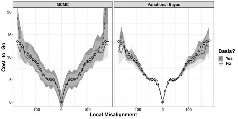
Figure 1: Estimated cost-to-go function for a Vicsek et al. (1995) SPP model using LMDP IRL for Bayesian MCMC sampling and variational approximation under known passive dynamics. The models either used Gaussian basis functions (dashed lines) or independent state parameters (solid lines). The shaded regions correspond to the 95% C.I. The open circles is the true cost-to-go function calculated from equation (12). The mean and true cost-to-go functions were shifted to have minimum 0.

The LMDP framework for IRL allows for efficient estimation of the state costs $r_{i}$ from the estimation of the cost-to-go by rearranging (12):

$$r_{i}=\text{log}(\lambda)+v_{i}+\text{log}\left(\sum_{j}\bar{p}_{ij}\textrm{exp}(-v_{j})\right),$$ (13)

for $i=1,...,J$. Figure 2 shows that the estimated costs from the mean cost-to-go functions in Figure 1 generally match the arbitrary state costs defined in (10).

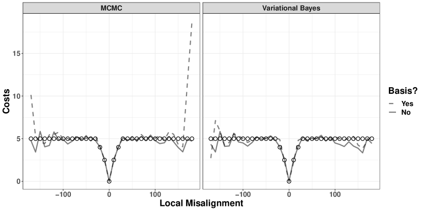
Figure 2: Estimated state costs for a Vicsek et al. (1995) SPP model using LMDP IRL for Bayesian MCMC sampling and variational approximation under known passive dynamics. The models either used Gaussian basis functions (dashed lines) or independent state parameters (solid lines). The open circles are the true state costs from (10).

For the MCMC estimation with bisquare basis functions, there is an increase in cost-to-go and uncertainty at the boundaries. The obvious spike at $180^{\circ}$ is the cost-to-go for the state defined by local misalignment less than $-175^{\circ}$ and greater than $175^{\circ}$. The Gaussian basis functions were not defined on a circle, but rather the continuous real line and could be contributing to the lack of smoothness near the boundary. Additionally, some flexibility is lost in estimation by reducing the dimensionality of the state space with the basis functions.

4 Guppy Application

We used the data publicly available from Bode et al. (2012) on an experiment involving a captive population of guppies (Poecilia reticulata). Groups of 10 same sex guppies were filmed from above in a square tank with one corner containing gravel and shade, which is defined by a point. The shaded corner provided shelter and is hypothesized to be attractive to the guppies. The guppies were released in the tank in the opposite corner. Bode et al. (2012) determined positions from video tracking software at a rate of 10 frames per second. The data made available by Bode et al. (2012) consist of movement trajectories truncated to the time points when all individuals were moving until one guppy reached the shaded target area; the range of time series was 20 - 285 frames. There were 26 experiments with 12 experiments consisting of all females and 14 males (Figure 3). We used trajectories from all experiments to estimate the cost-to-go functions based on movement headings.

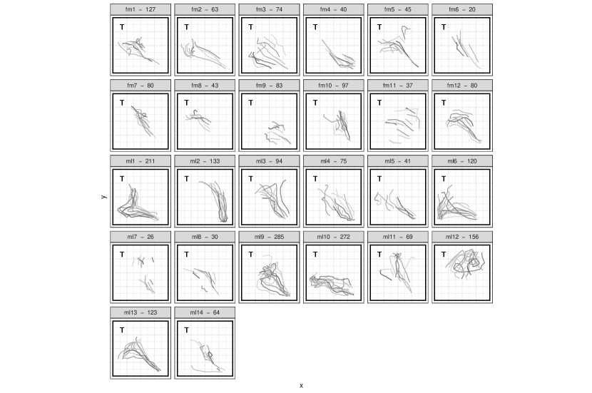
Figure 3: Trajectories of all 26 experiments of groups of 10 guppies in a tank. The target is located at the point marked “T.” The panel labels are “experiment number” - sample size. Experiments in first two rows are female (fm) groups and rows 3-5 are male (ml) groups.

We defined an LMDP for the guppy trajectories with a discrete state space of local misalignment and target misalignment. Local misalignment was defined as in Section 3 and target misalignment was defined as the difference between the current heading and the direction to the target point. We rescaled all pixel locations to the unit square and calculated the local misalignment between an individual and all other individuals. The assumption of interaction with all other agents is reasonable as the movement was bounded and there were no visual obstructions outside the target area (Bode et al., 2012). The two misalignment states were discretized using the same $36$ bins of length $10^{\circ}$ as in the previous section resulting in a discretized grid of $J=36\times 36$ states. We assume a fixed discount factor of 1 (i.e., all future costs/rewards are not discounted). For state transitions, we assumed synchronous updates as in the SPP simulation. Across the 26 experiments, there were 7,816 unique state transitions. Estimation of parameters in the guppy application was done by variational approximation due to the size of the state space.

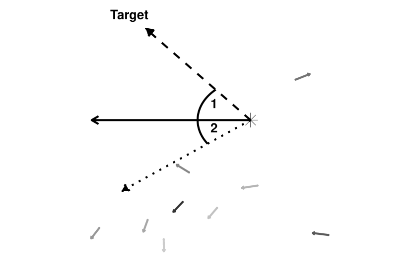
Figure 4: An illustration of the state for a guppy at the location marked by a star. The large solid arrow indicates the guppy’s heading. The dashed arrow indicates the straight-line direction from the guppy’s location and the angle marked by 1 is the guppy’s target misalignment (i.e., how much the guppy should change its current heading to face the target). The dotted line indicates the current average group direction as calculated from all of the solid arrows (including itself) and the angle marked by 2 is the guppy’s local misalignment (i.e., how much the guppy should change its current heading to head in the average direction). The angles labelled 1 and 2 would have opposite signs where turning angle 1 would result in a turn to the right and turning angle 2 would result in a turn to the left.

For the first set of estimated costs-to-go, we assumed the passive dynamics to be discrete uniform, (e.g., $\bar{p}_{ij}\propto 1$ for all $i,j=1,...,J$). The features, $\mathbf{X}$, considered were the identity matrix and 819 multiresolution bisquare basis functions generated uniformly within the gridded state space by the R package FRK (Zammit-Mangion, 2020) referred to as “Identity” and “Bisquare” respectively in Figure 5. The results shown in Figure 5 show a similar pattern among feature matrices with the bisquare basis functions providing more smoothing across the state space. In general, the results suggest the guppies perceived less cost for aligning with other guppies as the low costs-to-go in the center of the figure are concentrated around $0^{\circ}$ and there is more flexibility in target alignment as the low costs-to-go have more spread along the target misalignment axis. When comparing the two feature matrices (Figure 5), there is more contrast between the estimated cost-to-go function values estimated with bisquare basis functions than the identity matrix that is likely attributable to the dimension reduction.

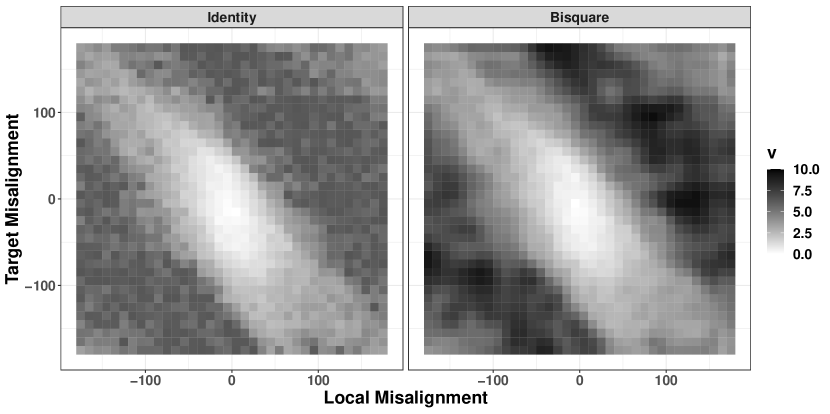
Figure 5: Variational posterior mean costs-to-go for the guppy experiments for a gridded state space of target and local misalignment across two sets of features: full (identity matrix) and bisquare basis functions. The passive dynamics are assumed to be discrete uniform and the mean estimated costs have been shifted to have a minimum of 0. A lower value associated with the legend for v indicates states with lower costs-to-go and therefore states to which the guppies are estimated to choose to transition.

To assess the sensitivity to the assumed passive dynamics, we estimated the costs-to-go under a set of passive dynamics corresponding to an independent, normal random walk on the gridded state space with standard deviation $90^{\circ}$. The standard deviation was chosen to be large enough to ensure all non-zero transition probabilities to use all of the observed data. The variational posterior mean and standard deviation for the costs-to-go are shown in Figure 6. Comparing to the previously estimated states, the variational posterior mean cost-to-go functions are similar. The variational posterior standard deviations reflect the pattern of observed frequencies with states more frequently observed having smaller uncertainty.

In Figures 5 and 6, the diagonal pattern can be attributed to the corners appearing far when plotted in the 2-D plane, but are close together in circular space so they have similar costs-to-go.

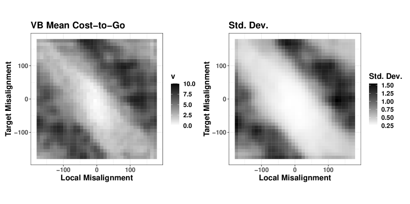
Figure 6: Variational posterior mean costs-to-go (left panel) and standard deviations (right panel) for the guppy experiments for a gridded state space of target and local misalignment with passive dynamics assumed to be a normal random walk and bisquare basis functions. The mean estimated costs-to-go have been shifted to have a minimum of 0. A lower value associated with the legend for v indicates states with lower costs-to-go and therefore states to which the guppies are estimated to choose to transition.

The marginal costs-to-go based on the estimates in Figure 6 are shown in Figure 7, where the costs-to-go are calculated as the mean across all values of the other state variable and shifted to have a minimum of 0. There is evidence of collective alignment as shown in the local misalignment costs-to-go function due to the minimum cost occurring at $0^{\circ}$ with gradual increase as misalignment increases in absolute value. Furthermore, the guppies appear to perceive local misalignments from $-15^{\circ}$ to $45^{\circ}$ as equally optimal, which can be contrasted with the sharp dip in cost-to-go for $0^{\circ}$ local misalignment in the SPP simulation Figure 1. The dip in the target misalignment cost-to-go function corresponds to the grid cells defined by $-55^{\circ}$ to $-45^{\circ}$ and $-45^{\circ}$ to $-35^{\circ}$, suggesting it is less costly to approach the upper corner with the target $55^{\circ}$ to $35^{\circ}$ to the right. From inspection of the observed data shown in Figure 3, it appears many of the guppies moved across the tank to the left first, which would require a right turn to decrease the target misalignment. A symmetry constraint could be applied to the costs-to-go by considering the absolute target alignment if it were assumed to be equally costly to approach from the right or left. Simulations of an example of guppy movement and estimated decision making from the costs-to-go in Figure 6 can be found at https://github.com/schafert/inverse-irl-guppy.

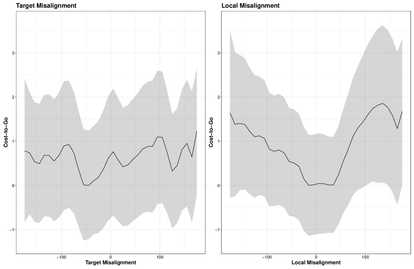
Figure 7: Marginal costs-to-go of target and local misalignment for the guppy experiments for a gridded state space of target and local misalignment with passive dynamics assumed to be a normal random walk and bisquare basis functions. The mean estimated costs have been shifted to have a minimum of 0. The lower costs-to-go increase the probability of transitioning into that state.

5 Discussion

Collective motion from generative local interaction rules limit possible behavior, but the (L)MDP framework extends the definition of the agent to include perception and internal processes (Ried, Müller and Briegel, 2019). By estimating the state costs-to-go or value functions, system specific local rules can be estimated.

Our analysis of the captive guppy populations confirms previous works that find evidence of social interactions between individuals (Bode et al., 2012; Russell, Hanks and Haran, 2016; McDermott, Wikle and Millspaugh, 2017). However, instead of defining a set of behavioral rules a priori, we estimated the decision-making mechanisms. Our results suggested the captive guppies value collective movement more than targeted movement toward shelter which was not previously explored by Russell, Hanks and Haran (2016) or McDermott, Wikle and Millspaugh (2017). Furthermore, the behavioral mechanisms determined by the cost-to-go functions were non-linear and non-symmetric.

In general, our inference is constrained to relative differences in costs-to-go. This is similar to the estimation of relative selection probabilities in animal resource selection modeling (Hooten et al., 2017, 2020) and therefore IRL can still provide useful inference. However, the SPP simulation demonstrated the ability to recover the magnitude of the true state costs and the true magnitude of the cost-to-go function.

It may be possible to improve the inference for the guppy data by relaxing the assumptions, estimating passive dynamics, and expanding the state space to include other features. We tested sensitivity of inference to choice of passive dynamics with two simple models. We did not detect a substantial difference, but for full quantification of uncertainty, joint estimation of passive dynamics could be considered. In future work, estimation of the passive dynamics parameters such as the random walk variance may be helpful. Additionally, the state space could include features based on physical distance to assess hypotheses about zonal collective movement which is a primary feature of collective movement ABMs (e.g., Couzin et al., 2002). A feature based on distance to target could similarly allow for interaction with the target to vary with location to relax the assumption that an individual interacts with the target in the same manner everywhere.

In the SPP simulation and guppy application, we assumed a discount factor of 1 which may be realistic for trajectories from such a short time frame. For observations spanning longer periods of time, it would be more realistic to assume there is some loss of memory about past states which would correspond to a discount factor less than 1. Additionally, the discount factor can also be interpreted as the degree to which agents behave optimally (Choi and Kim, 2014). It might be expected that observations from animals in the wild are subject to more stochasticity than experimental settings and therefore do not always behave optimally.

Another modeling choice was the grid size of the discrete state space. There is a precedence for discrete state spaces in animal movement modeling (Hooten et al., 2010; Hanks, Hooten and Alldredge, 2015). Biologically, the assumption of a discrete state space assumes the individual perceives values within the range of the bin as equally costly. For the guppy experiments, the evaluation of the state at a $10^{\circ}$ resolution could be adjusted given expert opinion or model based estimates of navigational ability (Mills Flemming et al., 2006).

There exist several avenues for extensions of the model to accommodate the behavior of free-ranging animals. First, alternative animal movement models could be proposed for the passive dynamics (Hooten et al., 2017). Second, covariates could be included on either the costs-to-go or passive dynamic models which would allow for heterogeneous decision making. Another interesting avenue would be to explore the methodology related to subtask completion for LMDPs (Earle, Saxe and Rosman, 2018). For example, a group of animals on the landscape navigating to a destination may require the completion of subtasks such as traversing wildlife corridors.

Appendix A LMDP Notation

The following is a table of LMDP notation used throughout the manuscript in order of appearance:

Symbol	Definition
$S$	Discrete state space with values $\{1,...,J\}$ and observations are denoted as $s$
$\bar{\mathbf{P}}$	$J\times J$ passive transition probability matrix
$\bar{p}_{ij}$	An element of $\bar{\mathbf{P}}$; passive transition probability from state $i$ to state $j$
$\gamma$	Discount factor in $[0,1]$
$R$	State cost function with values denoted $r_{i}$ for $i\in S$
$\mathbf{u}$	Continous controls which define the policy (1)
$u_{ij}$	An element of $\mathbf{u}$
$p_{ij}(u_{ij})$	Controlled transitions or policy defined by continuous controls and passive dynamics (1)
$p^{*}(s_{t}=j|s_{i}=i)$	Same as $p_{ij}(u_{ij})$
$l(\cdot,\mathbf{u})$	State and control cost function; it is the sum of the state cost $R$ and KL divergence between passive and controlled transition probabilities (2)
$\mathbf{v}$	Cost-to-go function or the expected discounted future state control costs (3) with values denoted by $v_{i}$ for $i\in S$

References

- Arora and Doshi (2018) {barticle}[author] \bauthor\bsnmArora, \bfnmSaurabh\binitsS. and \bauthor\bsnmDoshi, \bfnmPrashant\binitsP. (\byear2018). \btitleA survey of inverse reinforcement learning: Challenges, methods and progress. \bjournalarXiv preprint arXiv:1806.06877. \endbibitem
- Bellman (1957) {bbook}[author] \bauthor\bsnmBellman, \bfnmRichard\binitsR. (\byear1957). \btitleDynamic Programming, \bedition1 ed. \bpublisherPrinceton University Press, \baddressPrinceton, NJ, USA. \endbibitem
- Bode et al. (2012) {barticle}[author] \bauthor\bsnmBode, \bfnmNikolai WF\binitsN. W., \bauthor\bsnmFranks, \bfnmDaniel W\binitsD. W., \bauthor\bsnmWood, \bfnmA Jamie\binitsA. J., \bauthor\bsnmPiercy, \bfnmJulius JB\binitsJ. J., \bauthor\bsnmCroft, \bfnmDarren P\binitsD. P. and \bauthor\bsnmCodling, \bfnmEdward A\binitsE. A. (\byear2012). \btitleDistinguishing social from nonsocial navigation in moving animal groups. \bjournalThe American Naturalist \bvolume179 \bpages621–632. \endbibitem
- Carpenter et al. (2017) {barticle}[author] \bauthor\bsnmCarpenter, \bfnmBob\binitsB., \bauthor\bsnmGelman, \bfnmAndrew\binitsA., \bauthor\bsnmHoffman, \bfnmMatthew D\binitsM. D., \bauthor\bsnmLee, \bfnmDaniel\binitsD., \bauthor\bsnmGoodrich, \bfnmBen\binitsB., \bauthor\bsnmBetancourt, \bfnmMichael\binitsM., \bauthor\bsnmBrubaker, \bfnmMarcus\binitsM., \bauthor\bsnmGuo, \bfnmJiqiang\binitsJ., \bauthor\bsnmLi, \bfnmPeter\binitsP. and \bauthor\bsnmRiddell, \bfnmAllen\binitsA. (\byear2017). \btitleStan: A probabilistic programming language. \bjournalJournal of Statistical Software \bvolume76. \endbibitem
- Choi and Kim (2011) {binproceedings}[author] \bauthor\bsnmChoi, \bfnmJaedeug\binitsJ. and \bauthor\bsnmKim, \bfnmKee-Eung\binitsK.-E. (\byear2011). \btitleMap inference for Bayesian inverse reinforcement learning. In \bbooktitleAdvances in Neural Information Processing Systems \bpages1989–1997. \endbibitem
- Choi and Kim (2014) {barticle}[author] \bauthor\bsnmChoi, \bfnmJaedeug\binitsJ. and \bauthor\bsnmKim, \bfnmKee-Eung\binitsK.-E. (\byear2014). \btitleHierarchical Bayesian inverse reinforcement learning. \bjournalIEEE transactions on cybernetics \bvolume45 \bpages793–805. \endbibitem
- Couzin et al. (2002) {barticle}[author] \bauthor\bsnmCouzin, \bfnmIain D\binitsI. D., \bauthor\bsnmKrause, \bfnmJens\binitsJ., \bauthor\bsnmJames, \bfnmRichard\binitsR., \bauthor\bsnmRuxton, \bfnmGraeme D\binitsG. D. and \bauthor\bsnmFranks, \bfnmNigel R\binitsN. R. (\byear2002). \btitleCollective memory and spatial sorting in animal groups. \bjournalJournal of Theoretical Biology \bvolume218 \bpages1–11. \endbibitem
- Dvijotham and Todorov (2010) {binproceedings}[author] \bauthor\bsnmDvijotham, \bfnmKrishnamurthy\binitsK. and \bauthor\bsnmTodorov, \bfnmEmanuel\binitsE. (\byear2010). \btitleInverse Optimal Control with Linearly-Solvable MDPs. In \bbooktitleICML \bpages335-342. \endbibitem
- Earle, Saxe and Rosman (2018) {binproceedings}[author] \bauthor\bsnmEarle, \bfnmAdam C.\binitsA. C., \bauthor\bsnmSaxe, \bfnmAndrew M.\binitsA. M. and \bauthor\bsnmRosman, \bfnmBenjamin\binitsB. (\byear2018). \btitleHierarchical Subtask Discovery with Non-Negative Matrix Factorization. In \bbooktitleInternational Conference on Learning Representations. \endbibitem
- Finn, Levine and Abbeel (2016) {binproceedings}[author] \bauthor\bsnmFinn, \bfnmChelsea\binitsC., \bauthor\bsnmLevine, \bfnmSergey\binitsS. and \bauthor\bsnmAbbeel, \bfnmPieter\binitsP. (\byear2016). \btitleGuided cost learning: Deep inverse optimal control via policy optimization. In \bbooktitleInternational Conference on Machine Learning \bpages49–58. \endbibitem
- Hanks, Hooten and Alldredge (2015) {barticle}[author] \bauthor\bsnmHanks, \bfnmEphraim M.\binitsE. M., \bauthor\bsnmHooten, \bfnmMevin B.\binitsM. B. and \bauthor\bsnmAlldredge, \bfnmMat W.\binitsM. W. (\byear2015). \btitleContinuous-time discrete-space models for animal movement. \bjournalThe Annals of Applied Statistics \bvolume9 \bpages145 – 165. \bdoi10.1214/14-AOAS803 \endbibitem
- Hoffman and Gelman (2014) {barticle}[author] \bauthor\bsnmHoffman, \bfnmMatthew D.\binitsM. D. and \bauthor\bsnmGelman, \bfnmAndrew\binitsA. (\byear2014). \btitleThe No-U-Turn sampler: Adaptively setting path lengths in Hamiltonian Monte Carlo. \bjournalJournal of Machine Learning Research \bvolume15 \bpages1593-1623. \endbibitem
- Hooten, Scharf and Morales (2019) {barticle}[author] \bauthor\bsnmHooten, \bfnmMevin B.\binitsM. B., \bauthor\bsnmScharf, \bfnmHenry R.\binitsH. R. and \bauthor\bsnmMorales, \bfnmJuan M.\binitsJ. M. (\byear2019). \btitleRunning on empty: Recharge dynamics from animal movement data. \bjournalEcology Letters \bvolume22 \bpages377-389. \bdoi10.1111/ele.13198 \endbibitem
- Hooten, Wikle and Schwob (2020) {barticle}[author] \bauthor\bsnmHooten, \bfnmMevin\binitsM., \bauthor\bsnmWikle, \bfnmChristopher\binitsC. and \bauthor\bsnmSchwob, \bfnmMichael\binitsM. (\byear2020). \btitleStatistical Implementations of Agent-Based Demographic Models. \bjournalInternational Statistical Review. \bdoi10.1111/insr.12399 \endbibitem
- Hooten et al. (2010) {barticle}[author] \bauthor\bsnmHooten, \bfnmMevin B\binitsM. B., \bauthor\bsnmJohnson, \bfnmDevin S\binitsD. S., \bauthor\bsnmHanks, \bfnmEphraim M\binitsE. M. and \bauthor\bsnmLowry, \bfnmJohn H\binitsJ. H. (\byear2010). \btitleAgent-based inference for animal movement and selection. \bjournalJournal of Agricultural, Biological and Environmental Statistics \bvolume15 \bpages523–538. \endbibitem
- Hooten et al. (2017) {bbook}[author] \bauthor\bsnmHooten, \bfnmMevin B\binitsM. B., \bauthor\bsnmJohnson, \bfnmDevin S\binitsD. S., \bauthor\bsnmMcClintock, \bfnmBrett T\binitsB. T. and \bauthor\bsnmMorales, \bfnmJuan M\binitsJ. M. (\byear2017). \btitleAnimal Movement: Statistical Models for Telemetry Data. \bpublisherCRC Press. \endbibitem
- Hooten et al. (2020) {barticle}[author] \bauthor\bsnmHooten, \bfnmMevin B.\binitsM. B., \bauthor\bsnmLu, \bfnmXinyi\binitsX., \bauthor\bsnmGarlick, \bfnmMartha J.\binitsM. J. and \bauthor\bsnmPowell, \bfnmJames A.\binitsJ. A. (\byear2020). \btitleAnimal movement models with mechanistic selection functions. \bjournalSpatial Statistics \bvolume37 \bpages100406. \bnoteFrontiers in Spatial and Spatio-temporal Research. \bdoihttps://doi.org/10.1016/j.spasta.2019.100406 \endbibitem
- Jin et al. (2017) {binproceedings}[author] \bauthor\bsnmJin, \bfnmMing\binitsM., \bauthor\bsnmDamianou, \bfnmAndreas\binitsA., \bauthor\bsnmAbbeel, \bfnmPieter\binitsP. and \bauthor\bsnmSpanos, \bfnmCostas\binitsC. (\byear2017). \btitleInverse reinforcement learning via deep Gaussian process. In \bbooktitleConference on Uncertainty in Artificial Intelligence. \endbibitem
- Kangasrääsiö and Kaski (2018) {barticle}[author] \bauthor\bsnmKangasrääsiö, \bfnmAntti\binitsA. and \bauthor\bsnmKaski, \bfnmSamuel\binitsS. (\byear2018). \btitleInverse reinforcement learning from summary data. \bjournalMachine Learning \bvolume107 \bpages1517–1535. \endbibitem
- Kohjima, Matsubayashi and Sawada (2017) {binproceedings}[author] \bauthor\bsnmKohjima, \bfnmMasahiro\binitsM., \bauthor\bsnmMatsubayashi, \bfnmTatsushi\binitsT. and \bauthor\bsnmSawada, \bfnmHiroshi\binitsH. (\byear2017). \btitleGeneralized Inverse Reinforcement Learning with Linearly Solvable MDP. In \bbooktitleJoint European Conference on Machine Learning and Knowledge Discovery in Databases \bpages373–388. \bpublisherSpringer. \endbibitem
- Kucukelbir et al. (2015) {binproceedings}[author] \bauthor\bsnmKucukelbir, \bfnmAlp\binitsA., \bauthor\bsnmRanganath, \bfnmRajesh\binitsR., \bauthor\bsnmGelman, \bfnmAndrew\binitsA. and \bauthor\bsnmBlei, \bfnmDavid\binitsD. (\byear2015). \btitleAutomatic variational inference in Stan. In \bbooktitleAdvances in Neural Information Processing Systems \bpages568–576. \endbibitem
- Lee et al. (2017) {binproceedings}[author] \bauthor\bsnmLee, \bfnmKamwoo\binitsK., \bauthor\bsnmRucker, \bfnmMark\binitsM., \bauthor\bsnmScherer, \bfnmWilliam T\binitsW. T., \bauthor\bsnmBeling, \bfnmPeter A\binitsP. A., \bauthor\bsnmGerber, \bfnmMatthew S\binitsM. S. and \bauthor\bsnmKang, \bfnmHyojung\binitsH. (\byear2017). \btitleAgent-based model construction using inverse reinforcement learning. In \bbooktitle2017 Winter Simulation Conference (WSC) \bpages1264–1275. \bpublisherIEEE. \endbibitem
- McDermott, Wikle and Millspaugh (2017) {barticle}[author] \bauthor\bsnmMcDermott, \bfnmPatrick L\binitsP. L., \bauthor\bsnmWikle, \bfnmChristopher K\binitsC. K. and \bauthor\bsnmMillspaugh, \bfnmJoshua\binitsJ. (\byear2017). \btitleHierarchical nonlinear spatio-temporal agent-based models for collective animal movement. \bjournalJournal of Agricultural, Biological and Environmental Statistics \bvolume22 \bpages294–312. \endbibitem
- Mills Flemming et al. (2006) {barticle}[author] \bauthor\bsnmMills Flemming, \bfnmJ. E.\binitsJ. E., \bauthor\bsnmField, \bfnmC. A.\binitsC. A., \bauthor\bsnmJames, \bfnmM. C.\binitsM. C., \bauthor\bsnmJonsen, \bfnmI. D.\binitsI. D. and \bauthor\bsnmMyers, \bfnmR. A.\binitsR. A. (\byear2006). \btitleHow well can animals navigate? Estimating the circle of confusion from tracking data. \bjournalEnvironmetrics \bvolume17 \bpages351-362. \bdoihttps://doi.org/10.1002/env.774 \endbibitem
- Ng and Russell (2000) {binproceedings}[author] \bauthor\bsnmNg, \bfnmAndrew Y.\binitsA. Y. and \bauthor\bsnmRussell, \bfnmStuart J.\binitsS. J. (\byear2000). \btitleAlgorithms for Inverse Reinforcement Learning. In \bbooktitleICML \bpages663-670. \endbibitem
- Pinsler et al. (2018) {barticle}[author] \bauthor\bsnmPinsler, \bfnmRobert\binitsR., \bauthor\bsnmMaag, \bfnmMax\binitsM., \bauthor\bsnmArenz, \bfnmOleg\binitsO. and \bauthor\bsnmNeumann, \bfnmGerhard\binitsG. (\byear2018). \btitleInverse Reinforcement Learning of Bird Flocking Behavior. \bjournalICRA Swarms Workshop. \endbibitem
- Ramachandran and Amir (2007) {binproceedings}[author] \bauthor\bsnmRamachandran, \bfnmDeepak\binitsD. and \bauthor\bsnmAmir, \bfnmEyal\binitsE. (\byear2007). \btitleBayesian Inverse Reinforcement Learning. In \bbooktitleIJCAI \bvolume7 \bpages2586–2591. \endbibitem
- Ratliff, Bagnell and Zinkevich (2006) {binproceedings}[author] \bauthor\bsnmRatliff, \bfnmNathan D\binitsN. D., \bauthor\bsnmBagnell, \bfnmJ Andrew\binitsJ. A. and \bauthor\bsnmZinkevich, \bfnmMartin A\binitsM. A. (\byear2006). \btitleMaximum margin planning. In \bbooktitleProceedings of the 23rd International Conference on Machine Learning \bpages729–736. \endbibitem
- Ried, Müller and Briegel (2019) {barticle}[author] \bauthor\bsnmRied, \bfnmKatja\binitsK., \bauthor\bsnmMüller, \bfnmThomas\binitsT. and \bauthor\bsnmBriegel, \bfnmHans J\binitsH. J. (\byear2019). \btitleModelling collective motion based on the principle of agency: General framework and the case of marching locusts. \bjournalPLOS ONE \bvolume14. \endbibitem
- Russell, Hanks and Haran (2016) {barticle}[author] \bauthor\bsnmRussell, \bfnmJames C\binitsJ. C., \bauthor\bsnmHanks, \bfnmEphraim M\binitsE. M. and \bauthor\bsnmHaran, \bfnmMurali\binitsM. (\byear2016). \btitleDynamic models of animal movement with spatial point process interactions. \bjournalJournal of Agricultural, Biological and Environmental Statistics \bvolume21 \bpages22–40. \endbibitem
- Schafer, Wikle and Hooten (2021) {barticle}[author] \bauthor\bsnmSchafer, \bfnmToryn LJ\binitsT. L., \bauthor\bsnmWikle, \bfnmChristopher K\binitsC. K. and \bauthor\bsnmHooten, \bfnmMevin B\binitsM. B. (\byear2021). \btitleSupplement to ”Bayesian Inverse Reinforcement Learning for Collective Animal Movement”. \endbibitem
- Scharf et al. (2016) {barticle}[author] \bauthor\bsnmScharf, \bfnmHenry R.\binitsH. R., \bauthor\bsnmHooten, \bfnmMevin B.\binitsM. B., \bauthor\bsnmFosdick, \bfnmBailey K.\binitsB. K., \bauthor\bsnmJohnson, \bfnmDevin S.\binitsD. S., \bauthor\bsnmLondon, \bfnmJosh M.\binitsJ. M. and \bauthor\bsnmDurban, \bfnmJohn W.\binitsJ. W. (\byear2016). \btitleDynamic social networks based on movement. \bjournalAnn. Appl. Stat. \bvolume10 \bpages2182–2202. \bdoi10.1214/16-AOAS970 \endbibitem
- Scharf et al. (2018) {barticle}[author] \bauthor\bsnmScharf, \bfnmHenry R.\binitsH. R., \bauthor\bsnmHooten, \bfnmMevin B.\binitsM. B., \bauthor\bsnmJohnson, \bfnmDevin S.\binitsD. S. and \bauthor\bsnmDurban, \bfnmJohn W.\binitsJ. W. (\byear2018). \btitleProcess convolution approaches for modeling interacting trajectories. \bjournalEnvironmetrics \bvolume29 \bpagese2487. \bnotee2487 env.2487. \bdoi10.1002/env.2487 \endbibitem
- Sošić, Zoubir and Koeppl (2017) {barticle}[author] \bauthor\bsnmSošić, \bfnmAdrian\binitsA., \bauthor\bsnmZoubir, \bfnmAbdelhak M\binitsA. M. and \bauthor\bsnmKoeppl, \bfnmHeinz\binitsH. (\byear2017). \btitleA Bayesian approach to policy recognition and state representation learning. \bjournalIEEE Transactions on Pattern Analysis and Machine Intelligence \bvolume40 \bpages1295–1308. \endbibitem
- Sošić et al. (2017) {binproceedings}[author] \bauthor\bsnmSošić, \bfnmAdrian\binitsA., \bauthor\bsnmKhudaBukhsh, \bfnmWasiur R\binitsW. R., \bauthor\bsnmZoubir, \bfnmAbdelhak M\binitsA. M. and \bauthor\bsnmKoeppl, \bfnmHeinz\binitsH. (\byear2017). \btitleInverse Reinforcement Learning in Swarm Systems. In \bbooktitleProceedings of the 16th Conference on Autonomous Agents and MultiAgent Systems \bpages1413–1421. \endbibitem
- Sutton and Barto (1998) {bbook}[author] \bauthor\bsnmSutton, \bfnmRichard S\binitsR. S. and \bauthor\bsnmBarto, \bfnmAndrew G\binitsA. G. (\byear1998). \btitleIntroduction to reinforcement learning \bvolume2. \bpublisherMIT press Cambridge. \endbibitem
- Stan Development Team (2020) {bmisc}[author] \bauthor\bsnmStan Development Team (\byear2020). \btitleRStan: the R interface to Stan. \bnoteR package version 2.19.3. \endbibitem
- Todorov (2007) {binproceedings}[author] \bauthor\bsnmTodorov, \bfnmEmanuel\binitsE. (\byear2007). \btitleLinearly-solvable Markov decision problems. In \bbooktitleAdvances in Neural Information Processing Systems \bpages1369–1376. \endbibitem
- Todorov (2009) {barticle}[author] \bauthor\bsnmTodorov, \bfnmEmanuel\binitsE. (\byear2009). \btitleEfficient computation of optimal actions. \bjournalProceedings of the National Academy of Sciences \bvolume106 \bpages11478–11483. \endbibitem
- Vicsek et al. (1995) {barticle}[author] \bauthor\bsnmVicsek, \bfnmTamás\binitsT., \bauthor\bsnmCzirók, \bfnmAndrás\binitsA., \bauthor\bsnmBen-Jacob, \bfnmEshel\binitsE., \bauthor\bsnmCohen, \bfnmInon\binitsI. and \bauthor\bsnmShochet, \bfnmOfer\binitsO. (\byear1995). \btitleNovel type of phase transition in a system of self-driven particles. \bjournalPhysical Review Letters \bvolume75 \bpages1226. \endbibitem
- Wikle and Hooten (2016) {bincollection}[author] \bauthor\bsnmWikle, \bfnmChristopher K\binitsC. K. and \bauthor\bsnmHooten, \bfnmMevin B\binitsM. B. (\byear2016). \btitleHierarchical agent-based spatio-temporal dynamic models for discrete-valued data. In \bbooktitleHandbook of Discrete-Valued Time Series (\beditor\bfnmRichard A\binitsR. A. \bsnmDavis, \beditor\bfnmScott H\binitsS. H. \bsnmHolan, \beditor\bfnmRobert\binitsR. \bsnmLund and \beditor\bfnmNalini\binitsN. \bsnmRavishanker, eds.) \bpages349 – 366. \bpublisherChapman & Hall/CRC Press, \baddressBoca Raton, FL. \endbibitem
- Wulfmeier, Ondruska and Posner (2015) {barticle}[author] \bauthor\bsnmWulfmeier, \bfnmMarkus\binitsM., \bauthor\bsnmOndruska, \bfnmPeter\binitsP. and \bauthor\bsnmPosner, \bfnmIngmar\binitsI. (\byear2015). \btitleDeep inverse reinforcement learning. \bjournalarXiv preprint arXiv:1507.04888. \endbibitem
- Yamaguchi et al. (2018) {barticle}[author] \bauthor\bsnmYamaguchi, \bfnmShoichiro\binitsS., \bauthor\bsnmNaoki, \bfnmHonda\binitsH., \bauthor\bsnmIkeda, \bfnmMuneki\binitsM., \bauthor\bsnmTsukada, \bfnmYuki\binitsY., \bauthor\bsnmNakano, \bfnmShunji\binitsS., \bauthor\bsnmMori, \bfnmIkue\binitsI. and \bauthor\bsnmIshii, \bfnmShin\binitsS. (\byear2018). \btitleIdentification of animal behavioral strategies by inverse reinforcement learning. \bjournalPLoS Computational Biology \bvolume14 \bpagese1006122. \endbibitem
- Zammit-Mangion (2020) {bmanual}[author] \bauthor\bsnmZammit-Mangion, \bfnmAndrew\binitsA. (\byear2020). \btitleFRK: Fixed Rank Kriging. \bnoteR package version 0.2.2.1. \endbibitem
- Ziebart et al. (2008) {binproceedings}[author] \bauthor\bsnmZiebart, \bfnmBrian D.\binitsB. D., \bauthor\bsnmMaas, \bfnmAndrew\binitsA., \bauthor\bsnmBagnell, \bfnmJ. Andrew\binitsJ. A. and \bauthor\bsnmDey, \bfnmAnind K.\binitsA. K. (\byear2008). \btitleMaximum Entropy Inverse Reinforcement Learning. In \bbooktitleProceedings of the 23rd National Conference on Artificial Intelligence. \bseriesAAAI’08 \bvolume3 \bpages1433–1438. \bpublisherAAAI Press. \endbibitem