Simulating gamma-ray production from cosmic rays interacting with the solar atmosphere in the presence of coronal magnetic fields

Abstract

Cosmic rays can interact with the solar atmosphere and produce a slew of secondary messengers, making the Sun a bright gamma-ray source in the sky. Detailed observations with Fermi-LAT have shown that these interactions must be strongly affected by solar magnetic fields in order to produce the wide range of observational features, such as high flux and hard spectrum. However, the detailed mechanisms behind these features are still a mystery. In this work, we tackle this problem by performing particle-interaction simulations in the solar atmosphere in the presence of coronal magnetic fields modeled using the potential field source surface (PFSS) model. We find that the low-energy ($\sim$ GeV) gamma-ray production is significantly enhanced by the coronal magnetic fields, but the enhancement decreases rapidly with energy. The enhancement is directly correlated with the production of gamma rays with large deviation angles relative to the input cosmic-ray direction. We conclude that coronal magnetic fields are essential for correctly modeling solar disk gamma rays below 10 GeV, but above that the effect of coronal magnetic fields diminishes. Other magnetic field structures are needed to explain the high-energy disk emission.

I Introduction

The Sun is a high-energy astrophysical source due to its interactions with cosmic rays: Cosmic-ray electrons inverse-Compton scatter with sunlight and produce a diffuse gamma-ray halo around the Sun Orlando and Strong (2007); Moskalenko et al. (2006); Orlando and Strong (2013); Cosmic-ray nuclei interact with the solar atmosphere hadronically, and produce secondary gamma rays and neutrinos Moskalenko et al. (1991); Seckel et al. (1991); Moskalenko et al. (1991); Ingelman and Thunman (1996). The latter component is mainly emitted from the photosphere, thus is more concentrated than the inverse-Compton halo; we denote it as the solar disk emission.

The solar disk gamma-ray emission was first detected with EGRET Thompson et al. (1997); Orlando and Strong (2008) and later with Fermi-LAT with much better precision Abdo et al. (2011). The observed emission is higher than early estimates by almost an order of magnitude Seckel et al. (1991). Subsequent analyses with six years Ng et al. (2016) and nine years of Fermi data Linden et al. (2018); Tang et al. (2018) have found several new features, including: 1) The flux anticorrelates with solar activity at low energies ($\sim$ 1 GeV) as well as at the highest detected energy ($\sim$ 100 GeV) with a much larger correlation amplitude; 2) The flux exhibits a hard spectral index ($\sim E^{-2.2}$) and reaches up to at least 200 GeV during solar minimum; 3) A spectral dip around 30–50 GeV; 4) The morphology of the solar emission varies strongly as a function of the solar cycle. See Ref. Nisa et al. (2019) for a brief overview. These signatures are all unexplained, and suggest that the disk emission is significantly affected by solar magnetic fields. It is still an open problem on how magnetic fields facilitate the production of the observed solar gamma rays and its features.

Because the $>100$ GeV gamma-ray emission is highly variable, and has a hard spectrum during solar minimum, very-high-energy observation of the Sun is another valuable avenue for probing the underlying physics. Only large ground-based air-shower array experiments, such as ARGO-YBJ, HAWC, and LHAASO can observe the Sun at TeV energies. ARGO-YBJ has provided the first set of strong constraints on sub-TeV to 10 TeV emission during the quiet Sun period from 2008–2010 Bartoli et al. (2019). HAWC was able to provide a stronger constraint Albert et al. (2018a) using data from November 2014 to December 2017. However, the Sun was more active in that period, thus the high-energy spectrum is expected to be soft from Fermi observations. IceCube has performed the first dedicated search of solar atmospheric neutrinos Aartsen et al. (2019a), but the sensitivity is still above the predicted flux Argüelles et al. (2017); Edsjo et al. (2017).

The first detailed computation of the solar disk gamma-ray flux was performed by Seckel, Stanev, and Gaisser Seckel et al. (1991), who proposed that charged cosmic rays entering the atmosphere are reflected by concentrated magnetic flux tubes, and thus enhances the gamma-ray production compared to the zero-magnetic field case. Until recently, calculations that focus on gamma rays Zhou et al. (2017); Gao et al. (2018) and neutrinos Ingelman and Thunman (1996); Argüelles et al. (2017); Edsjo et al. (2017) all ignored magnetic fields. In Ref. Zhou et al. (2017), the minimum disk emission from the Sun limb was estimated with zero-magnetic field calculations, and in Ref. Linden et al. (2018), the maximum was estimated by assuming all cosmic rays are reflected on the solar surface and produce gamma rays with 100% efficiency. However, none of the calculations can explain the observations, such as the flux, spectral shape, time variability, etc.

In this work, as a first step to understand the phenomenologies behind cosmic rays interacting with the Sun, we study the production of solar disk emission using the particle simulation toolkit, Geant4, together with the observation-based PFSS magnetic-field model.

II Simulation setup

II.1 The Geant4 Toolkit

Geant4 is a software toolkit that simulates the passage of particles through matter Allison et al. (2016). Due to its powerful functionality and modeling capability, Geant4 is used in many applications, such as high-energy physics, nuclear physics, medical science, and space science. We base our computation on version 10.3.3.

A typical Geant4 simulation contains many components, such as detector designation, event generator, particle definition, and physics models. We focus on the energy range between 100 MeV and 100 TeV, which covers the energy range of Fermi and HAWC. To model both hadronic and electromagnetic interactions, we use the FTFP-BERT physics list. Below 5 GeV, the Bertini cascade model Heikkinen et al. (2003) is used. With a transition between 4-5 GeV, the Fritiof string model is used above 4 GeVJulia Yarba .

Magnetic fields are included in Geant4 through a separate class. Following the Geant4 guide, we compute the particle tracks using the default Runge-Kutta method.

II.2 The G4SOLAR code

Based on the Geant4 toolkit, we develop G4SOLAR, a program that handles particle propagation and particle interactions in the solar atmosphere. In this section, we describe the essential components of G4SOLAR.

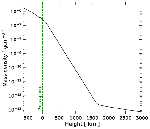
Figure 1: The density profile of the Sun near the photosphere Seckel et al. (1991); Norman H. Baker, Stefan Temesváry (1966); White, Marvin L. and Kim, Koo Sun (1966).

II.2.1 Solar atmosphere

The atmosphere of the Sun consists of the photosphere, the chromosphere, and the corona Wiegelmann et al. (2014). The photosphere, with roughly 500 km thickness, is the layer where the Sun becomes optically opaque. The chromosphere is the region roughly a few thousand km above the photosphere; and the corona is defined as the large region above the chromosphere, where the temperature rises to millions of kelvin.

Figure 1 shows the density distribution of the solar atmosphere used in our calculation. Below the photosphere (set at 0 km), we use the density provide by Ref. Norman H. Baker, Stefan Temesváry (1966), and we use Eq. (2.1) of Ref. Seckel et al. (1991) to extend it to 1600 km. Between 1600 to 3000 km, we use the data in Ref. White, Marvin L. and Kim, Koo Sun (1966). We configure the Sun as a sphere and divide the region from -600 km to +3000 km into 3600 equal-thickness layers following the density profile shown in the figure.

II.2.2 Solar magnetic fields

For magnetic fields near the Sun, we consider the potential field source surface (PFSS) model Schatten et al. (1969); Altschuler and Newkirk (1969); Hoeksema (1984); Wang and Sheeley (1992), which describes the large-scale magnetic fields above the photosphere, $R_{\odot}$. Using the photospheric magnetic-field measurement as a boundary condition, and assuming that the current density is zero as well as the fields are completely radial at a distance, $R_{ss}\sim{\cal O}(1)R_{\odot}$, the magnetic fields between $R_{\odot}$ and $R_{ss}$ can be computed by solving for the scalar potential. Thus, for each complete Carrington cycle ($\sim 27$ days), using the photospheric measurements by observatories such as GONG , and SOHO/MDI , a PFSS model can be obtained with only $R_{ss}$ as a free parameter, which is fitted separately. We note that the large-scale magnetic fields we consider are drastically different from the small-scale magnetic flux tube used by Seckel et al. Seckel et al. (1991); we compare with their results in detail in Sec. III.7. The PFSS model is easy to implement and was found to agree reasonably well with more detailed and computationally expensive magnetohydrodynamic models Riley et al. (2006), thus making it a natural choice for our simulation study.

The PFSS models are obtained using the Solar Software (SSW) package . We consider the Carrington Rotations 2070 (13 May 2008 to 9 Jun 2008) for solar minimum and 2149 (07 Apr 2014 to 04 May 2014) for solar maximum. The source surface parameter is chosen to be 1.6$R_{\odot}$ for solar minimum, 2.5$R_{\odot}$ for solar maximum. Hereafter, we denote the solar minimum case as Quiet, the solar maximum case as Active, and the control case with zero magnetic field as NoField.

We evaluate the PFSS model in a 361 (radial) $\times$ 180 (polar) $\times$ 360 (azimuthal) grid in our simulation volume. We note that typically the PFSS model starts at the photosphere. For our purpose, we extrapolate the PFSS model down to 600 km below the photosphere. Because we start our simulation at +3000 km, we also practically ignore all the magnetic fields above this height. During simulation, the value of the magnetic fields at each point in the simulation volume is then obtained by interpolating these grid points.

Table 1: The mean values for the three components of the PFSS magnetic fields and their standard deviations for Quiet and Active cases, evaluated at the photosphere.

	$<B_{r}>~{}[G]$	$<B_{\theta}>~{}[G]$	$<B_{\phi}>~{}[G]$
Quiet	0.03 $\pm$ 2.16	0.11 $\pm$ 2.22	-1.04 $\pm$ 2.45
Active	-0.35 $\pm$ 15.42	0.66 $\pm$ 15.46	0.77 $\pm$ 2.54

Table  1 shows the mean values of the magnetic fields and their standard deviations for the two phases of solar activity with the PFSS model. We obtain the mean and the deviation values by sampling 100,000 points randomly at the photosphere. These values are stable versus height. Changing the sampling point between -600 km and +3000,km change the values by a few percent. In general, the mean values are close to zero, which is due to averaging regions with magnetic fields of opposite directions. The standard deviation is thus more representative of the typical field strength of the model, which is $\simeq 2$ G for the Quiet case. For the Active case, however, the standard deviation is much larger, $\simeq 15$ G for the $r$ and $\theta$ component.

II.2.3 Particle sampling

The final component of G4SOLAR is the position and direction sampling of the cosmic-ray particles. The starting position of the input particles are first sampled uniformly at 3000 km above the photosphere. We consider the energy between 100 MeV and 100 TeV, which is divided uniformly into six logarithmic intervals. For each interval, the energy is sampled with a spectral index -1 (uniform in log.), and have sampling size varies due to computational time consideration, with the number of particles between $10^{5}$ and $10^{6}$.

The momentum vectors of the particles at the input position also need to be sampled. We define the incident angle, $\omega_{p}$, as the angle between the momentum vector and the normal direction of the spherical simulation volume at particle position (see Sec. III.5). The number of particles is then sampled according to $N\propto\sin\omega_{p}\cos\omega_{p}$. Here $\sin\omega_{p}$ is the solid angle factor and $\cos\omega_{p}$ takes into account the geometric factor between the incoming cosmic-ray flux and the receiving surface element. The azimuthal direction of the particles are sampled uniformly. In our setup, only events with $\omega\geq 90^{\circ}$ can enter and interact with the Sun, we thus only sample in the range between $90^{\circ}$ and $180^{\circ}$.

All the particles are tracked only when they are in the simulation volume. Thus, for particles leaving the -600 km layer, we assume they are completely absorbed; for particles leaving the 3000 km layer, we assume they have escaped. The simulation results thus consist of all the escaped gamma-ray events.

II.3 Cosmic-ray spectrum and output flux

To connect the simulation results to real world situations, the cosmic-ray spectrum is required. It is well-known that the Sun can change the cosmic-ray propagation environment in the solar system Gleeson and Axford (1968), and modulate the cosmic-ray flux as they propagate inward from the interstellar space. It is thus natural to expect additional modulation exist when cosmic rays propagate from Earth orbit to the vicinity of the Sun. However, cosmic-ray propagation in the solar system is still an open problem Potgieter (2013), and is likely important only at low energies. For simplicity, we use the cosmic-ray spectrum measured at the Earth position and defer the inclusion of solar modulation for future works.

We set the composition of the Sun to be 100% protons, and only consider cosmic-ray protons. Including heavier species, such as Helium, would increase the gamma-ray flux by less than a factor of 2 Zhou et al. (2017), which is a relatively small correction factor considering other uncertainties, such as solar magnetic field models.

We use the 2006 proton spectrum by PAMELA Adriani et al. (2013) from 0.1 MeV to 45 GeV, then AMS-02 Aguilar et al. (2015) from 45 GeV to 2.5 TeV, and finally CREAM Yoon et al. (2011) up to 100 TeV. The final photon flux is then obtained by weighting the cosmic-ray spectrum with the simulation spectrum event by event, and then divided by the Earth–Sun distance squared.

III Simulation Results

III.1 Zero magnetic field case

We first consider the NoField case as a cross check and validation of the simulation procedure. The simulation and analysis are performed without magnetic fields, otherwise keeping all procedures identical to the cases with magnetic fields.

Figure 2 shows the results for the NoField case. We compare with the semi-analytic calculation by Zhou et al. Zhou et al. (2017), where they assumed that the incoming cosmic rays and the gamma rays produced are collinear. With this approximation, only cosmic rays that point at the Earth and graze through the edge of the solar atmosphere can produce detectable gamma rays (Sun limb). This limb flux can be easily calculated as it is a 1D computation; the resultant flux roughly follows the cosmic-ray spectral index. We find that our NoField results agree well with Zhou et al. above 10 GeV, meaning that the collinear approximation is appropriate here. Below 10 GeV the NoField case has much higher gamma-ray production, which is caused by large-angle gamma-ray events. We discuss this in more detail in Sec. III.5.1. Above a few TeV, we start to see deviations due to the imposed cosmic-ray energy cutoff at 100 TeV.

We also compare our results with Gao et al. Gao et al. (2018), the precursor of this work, where the cosmic-ray position sampling step was not implemented due to the spherical symmetry of the problem when magnetic fields are not included. We find that our results agree well with each other. This validates our 3D position and angle sampling procedures described in Sec. II.1, which are necessary once global solar magnetic fields are introduced.

III.2 Results with magnetic fields

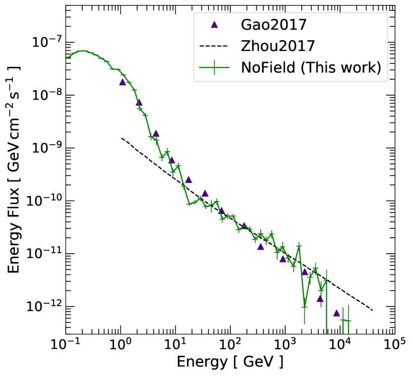
Figure 2: Simulated solar disk gamma-ray flux without magnetic fields (NoField). For comparison, we also show the 1D semi-analytic calculation by Zhou et al. Zhou et al. (2017), and the simplified Geant4 simulation result by Gao et al. Gao et al. (2018). The enhanced gamma-ray production below 10 GeV is due to large-angle events caused by kinematics. See Sec. III.5.1 for details.

Figure 3 shows the solar disk gamma-ray flux for Quiet and Active together with that for NoField. We find that the the PFSS magnetic fields can dramatically change the gamma-ray production. At 100 MeV, all three cases have similar flux. Between 100 MeV and 10 GeV, though, both Quiet and Active exhibit harder spectral shapes and have higher flux than the NoField case. The difference in flux is the largest at around 10 GeV, by almost two orders of magnitude. Above 10 GeV, the spectra fall sharply, and have spectral shapes even softer than the cosmic-ray spectrum. Around 1 TeV, the Quiet flux and Active flux merge with the NoField flux, showing that the PFSS magnetic fields can no longer affect the gamma-ray production. We interpret these observations using the event angular distributions in Sec. III.5.2.

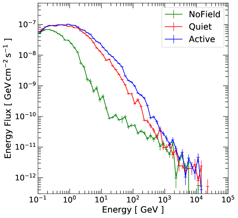
Figure 3: Solar disk gamma-ray flux computed by G4SOLAR without magnetic fields (NoField), with solar minimum PFSS magnetic fields (Quiet), and with solar maximum PFSS magnetic fields (Active). The magnetic fields boost the gamma-ray production by enhancing the production of large-angle events. See Sec. III.5.2 for details.

Comparing the results between Quiet and Active, the two fluxes have similar shapes, except that the Active flux becomes larger by about a factor of two in 1 GeV to 1 TeV.

In the next few subsections, we explore in detail the simulation results and attempt to understand various properties of these results.

III.3 Physical Processes

Figure 4 shows the breakdown of the physical processes that contribute to the solar disk gamma-ray production. For all three cases, we find that the dominant contribution comes from neutral pion ($\pi^{0}$) decays. These pions could be produced directly from the primary proton interactions, or from the subsequent hadronic showers. Due to the short lifetime of $\pi^{0}$, they decay promptly before undergoing additional scatterings. As a result, $\pi^{0}$ can efficiently convert the primary proton energy into gamma rays.

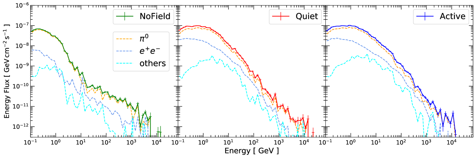
Figure 4: The breakdown of the total flux into the physical processes that are responsible for the gamma-ray production. The dominant process is neutral pion decays, then followed by electron/positron bremsstrahlung and annihilation, and finally miscellaneous processes that include decay of heavier hadron states, etc. See text for details.

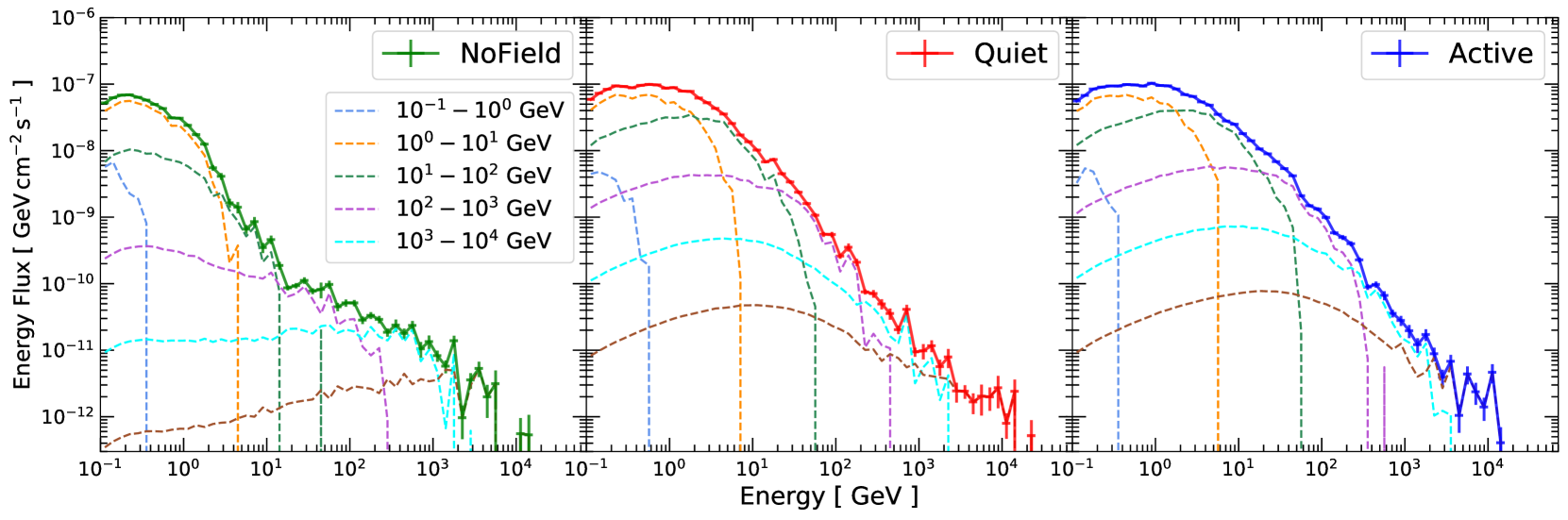
Figure 5: The breakdown of the total flux into the contributions from the corresponding input proton energy intervals. Vertical lines correspond to isolated nonzero energy bins.

The second most important source of gamma rays, at $\sim$ 10% level, comes from electron and positron bremsstrahlung as well as positron annihilation (labelled simply as $e^{+}e^{-}$). These electrons and positrons come from the final states of many secondaries (e.g., $\pi^{\pm}$), or they can be produced from electromagnetic showers initiated by energetic gamma rays or electrons.

Finally, we group the remaining gamma-ray production channels into “others”, which includes decays of heavier hadron states (e.g., $\eta,\Sigma,\Omega$, etc), hadron inelastic scatterings, muon-bremsstrahlung, etc. These contributions are subdominant, but not negligible.

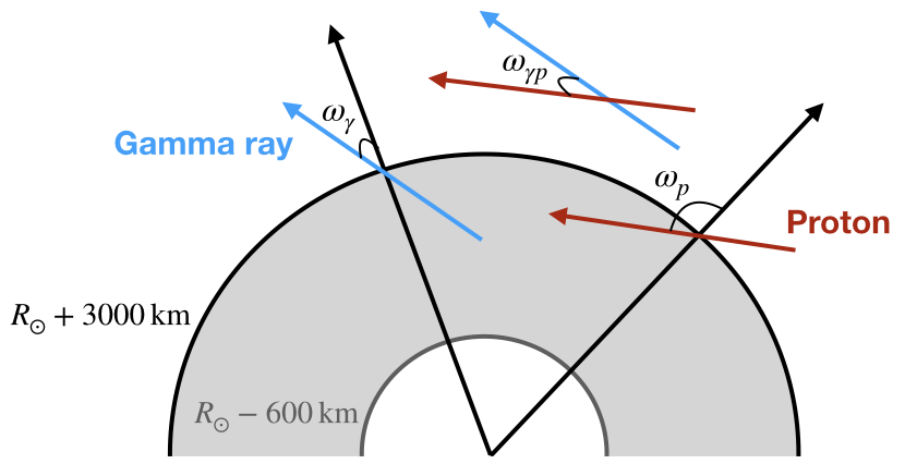
Figure 6: The definitions of the angles considered in Sec. III.5. Schematically, the grey region highlights the simulation volume. The black arrow is the normal direction from the center of the Sun and the dark red (blue) arrow is the proton (gamma-ray) velocity vector.

III.4 Energy contribution

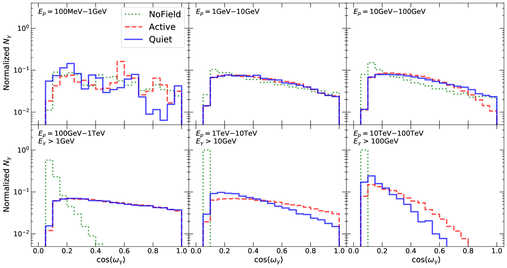
Figure 7: The angular distribution of the gamma rays produced in NoField, Quiet, and Active. $\cos(\omega_{\gamma})=1$ corresponds to the radially outward direction and $\cos(\omega_{\gamma})=0$ corresponds to the tangential direction. Each panel correspond to an interval of the input proton energies, and the distributions are all renormalized to have the same area. For display purpose, gamma-ray energy cuts are applied in the bottom three panels. Comparing between NoField and the results with magnetic fields, the gamma-ray angular distribution is significantly widened at high energies.

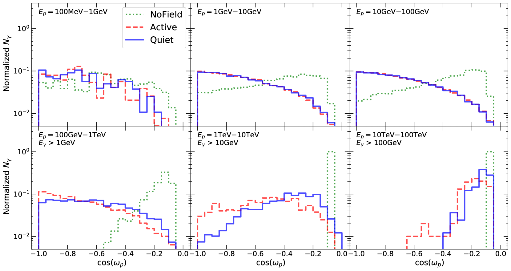
Figure 8: The angular distribution of the incoming protons that have successfully produced an outgoing photon. $\omega_{p}$ is defined as the angle between the proton velocity vector and the normal direction of the simulation volume at the proton injection position.

Figure 9: The distribution of the angle between each pair of incoming protons and outgoing gamma rays, $\omega_{\gamma p}$.

Figure 5 shows the contributions from each input proton energy intervals to the total gamma-ray flux. Interestingly, for proton energies 0.1 GeV to 10 GeV, we find no significant changes in the contribution between NoField and those with magnetic fields. Most of the flux enhancements for Quiet and Active come from proton energies from 10 GeV to 1 TeV, where the low energy “tails” in the NoField case change into “bumps” in the cases with magnetic fields. From 1 TeV to 100 TeV, while the gamma-ray production is enhanced, the enhancements are mainly at low energies, which are buried by the other low-proton-energy components and have little effect to the final results.

III.5 Event angular distribution

We explore in detail the angular distribution of protons that interact in the solar atmosphere as well as that of the outgoing gamma rays, which we find helpful in elucidating the the physics behind the enhanced gamma-ray production with magnetic fields. We consider three angles, $\omega_{p}$, $\omega_{\gamma}$, and $\omega_{\gamma p}$, which are illustrated schematically in Fig 6.

Figure 7 shows the angular distribution of the outgoing gamma rays. We define the angle $\omega_{\gamma}$ as the angle between the vector of the escaped gamma rays and the normal direction of the spherical simulation volume, evaluated at +3000 km above the photosphere. In other words, $\cos(\omega_{\gamma})$ = 1, 0 correspond to gamma rays pointing radially outward and tangential to the simulation volume, respectively.

Similarly, Figure 8 shows the angular distribution for the incoming protons, where the angle $\omega_{p}$ is defined by the angle between the proton vector and the normal direction at +3000 km. We note that here we only consider protons that have successfully produced at least one escaped photon; protons that are completely absorbed or escaped without producing gamma rays are not included here.

And finally, Figure 9 shows the distribution for $\omega_{\gamma p}$, defined as the angles between the outgoing gamma rays and the incoming protons that produce gamma rays. Each proton could contribute multiple outgoing photons; all these pairs are considered in the distribution.

We note that for high proton energies, a large number of lower-energy gamma rays are produced, which are not important to the problem at hand, as shown in Sec. III.4. Therefore, to highlight the angular distribution for the relevant photons, we apply gamma-ray energy cuts $E_{\gamma}>1$GeV, $E_{\gamma}>10$GeV, and $E_{\gamma}>100$GeV for the three proton energy intervals above 100 GeV, respectively.

III.5.1 Distribution without magnetic fields

It is instructive to first consider the NoField case. At high energies ($E_{p}>100$ GeV), we find that the distributions tend towards $\omega_{\gamma}\simeq 90^{\circ}$, $\omega_{p}\simeq 90^{\circ}$, and $\omega_{\gamma p}\simeq 0^{\circ}$. This peaked angular distribution appear naturally due to the large Lorentz factor (except for the low-energy secondary photons that are cut from the figures). This corresponds to the Sun-limb scenarios, as discussed in Ref. Zhou et al. (2017).

However, for lower energy protons, we find that the distribution become significantly broader. Because there are no magnetic fields to change the trajectories of the particles, the broader distribution must be caused by mildly-relativistic scattering kinematics or multiple small-angle scatterings. We defer more detailed identification of the responsible particles and the interactions to future works.

The broader angular distribution can also explain the difference between the calculations from Zhou et al. Zhou et al. (2017) and the simulation results from this work and Gao et al. Gao et al. (2018). With the 1D approximation used in Zhou et al., gamma rays produced by protons with steep incident angles are all absorbed. However, as shown in our 3D calculation, e.g., the $\omega_{p}$ distribution in 1 GeV-100 GeV, the distribution is broad and even down-going protons ($\omega_{p}\sim 180^{\circ}$) can produce observable gamma rays. This is also precisely the proton energy range responsible for the enhanced gamma-ray flux ($E_{\gamma}\sim 1$ GeV) in our simulation compared to that by Zhou et al. Therefore, we conclude that by kinematic effects alone, proton-proton scattering can produce large-angle events; and these large angle events are responsible for enhancing the gamma-ray production around 1 GeV. At higher energies, as gamma rays and protons become more collinear, the 3D and 1D calculations produce similar results.

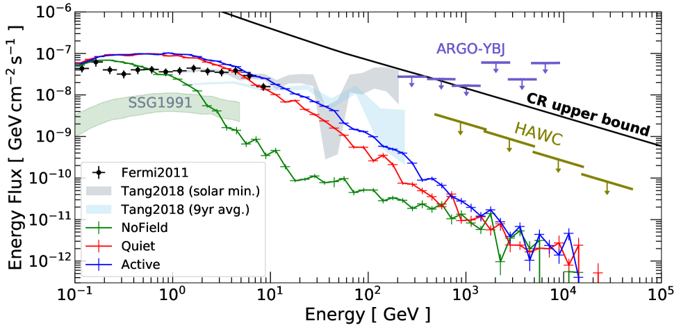
Figure 10: Our simulation results (NoField, Quiet, and Active) compared with solar disk observations from the 1.5-yr analysis by the Fermi collaboration Abdo et al. (2011), follow-up analysis with a similar period by Tang et al. Tang et al. (2018), and their 9-yr averaged results. We also show the prediction from Seckel et al. Seckel et al. (1991) (SSG1991), and the theoretical upper bound from Linden et al. Linden et al. (2018). The upper limits at high energies comes from ARGO-YBJ Bartoli et al. (2019) and HAWC Albert et al. (2018a).

III.5.2 Distribution with magnetic fields

Comparing the angular distributions of NoField with that from Quiet and Active, we see that the PFSS magnetic fields have a significant impact on the distribution. This is expected as both the directions of the primary protons and the charged secondaries ($\pi^{\pm}$, $e^{\pm}$, etc) are bent as they propagate in the simulation volume. The bending effect is evidently shown in the $\omega_{p}$ distribution. Importantly, as the NoField distribution becomes more peaked for $E_{p}>100$ GeV, the distribution with magnetic fields remain broad until $E_{p}>10$ TeV. Following the observations from the previous section, the broader distribution is responsible for the enhanced gamma-ray production compared with the NoField case. We conclude that the broadening of the angular distributions, caused by magnetic fields bending the cosmic-ray primaries and secondaries, can enhance the solar gamma-ray production.

Finally, comparing between the Quiet and Active results, we find that the Active angular distribution has more large-angle contributions than that for Quiet. This also explains why our simulation results find that the Active flux is larger than the Quiet flux around 10 GeV-1 TeV. This follows from Tab. 1, where Active have higher typical magnetic fields than Quiet, thus leading to more magnetic bendings. On the other hand, the Quiet result is similar to the Active result around 1 GeV. This suggests that below 1 GeV, larger magnetic fields does not further enhance the gamma-ray production, which is also shown by the similar $\omega_{\gamma p}$ distribution for proton energy between 1 GeV and 100 GeV. In other words, the magnetic-field enhancement effect saturates.

III.5.3 Estimating the Gyroradius

It is instructive to estimate the gyroradius, which puts the length and energy scales into perspective. The shortest length scale of our simulation is in the radial direction, 3600 km. Setting this as the gyroradius and consider 10 G as a typical field strength (Sec. II.2.2), the critical energy is

$$E_{c}\simeq{\rm 1\,TeV}\left(\frac{r}{3600\,{\rm km}}\right)\left(\frac{B}{10\,{\rm G}}\right)\,.$$ (1)

This means that it is possible for protons with energies below $E_{c}$ to undergo a complete reversal in their pointing direction in the simulation volume. Above $E_{c}$, one would then expect the effect of magnetic fields to decrease and approach the collinear limit. Indeed, this is consistent with observations from Figs. 8 and 9, where we can see that the angular distributions undergo a qualitative change below and above TeV.

III.6 Comparison with observations

Figure 10 shows our simulated solar disk emission together with observational results and constraints. We show the $\simeq$ 1.5-year result (Aug. 2008 – Feb. 2010) obtained by the Fermi collaboration Abdo et al. (2011) and the $\simeq$ 1.5-year result (Aug. 2008 – Jan. 2010) obtained by Tang et al. Tang et al. (2018) that extended the analysis to higher energy. During these periods, the Sun is dominantly in quiet states, which we simply denote as solar minimum. We also show the 9-year analysis (Aug. 2008 – Jul. 2017) by Tang et al. that covers both periods of low and high solar activities.

At low energies, between 0.1 GeV and 10 GeV, our results with magnetic fields are comparable to the solar minimum flux up to a factor of 2. Interestingly, Fermi observation suggests that the flux at this energy range anti-correlates with the solar activities Ng et al. (2016); Tang et al. (2018), which is not seen in the simulation result. This suggests additional physics is at play. One possibility is solar modulation in the inner solar system, which has the correct time variability, as the cosmic-ray flux is smaller when the Sun is more active. In short, the PFSS magnetic fields alone mildly over-produces the flux at this energy range, and cannot capture the time variability.

At higher energies, our results fall below the data quickly. At 100 GeV, both the Quiet and Active results is about 1 order of magnitude less than the observation. In particular, the spectrum of solar minimum observation was found to be hard until at least 200 GeV with no signs of cutoff, making the disagreement with our results even larger. For the 9-year averaged spectrum, which is dominated by periods of higher solar activity, the spectrum softens rapidly above 100 GeV, and could potentially fall into agreement with our calculations. The quality of measurement, however, is not sufficient to draw conclusive statements yet. Lastly, we also do not see the extreme time variability in the $>100$ GeV photon flux and the spectral dip around 30-50 GeV Linden et al. (2018); Tang et al. (2018). Thus, new magnetic fields or new physics ingredients must be needed, in addition to coronal fields, to explain the high-energy photon flux.

Above the Fermi-LAT energy range, only large ground-based air shower gamma-ray observatories can potentially detect high-energy gamma rays from the Sun. We show the upper limits from ARGO-YBJ Li et al. (2019) and HAWC Albert et al. (2018a), both orders of magnitude higher than our calculation. For reference, we also show the theoretical upper limit from cosmic rays interacting with the atmosphere Linden et al. (2018). Given that the solar minimum flux measurement by Fermi did not exhibit a cutoff, a detection could be possible with HAWC or LHAASO. TeV detection or constraint will be essential for identifying the mechanism responsible for the high-energy flux.

III.7 Comparison with other calculations with magnetic fields

For many years, the only solar disk gamma-ray calculation that took into account magnetic fields was the pioneer work by Seckel, Stanev, and Gaisser (SSG1991 Seckel et al. (1991)). In SSG1991, cosmic-ray propagation in the solar system was taken into account, and more importantly, cosmic rays entering the solar atmosphere were assumed to be funneled into magnetic flux tubes, and then reflected in the flux tubes due to the large field gradient. As a result, the gamma-ray production is enhanced by having the possibility of cosmic rays interacting after being reflected. However, even with such an enhancement, the SSG1991 model prediction is still much lower than the observation. Interestingly, in this work we find that at low energies, scattering kinematics and coronal magnetic fields can provide more than enough boost to the gamma-ray production. Thus, we find that the SSG1991 flux-tube reflection may be a subdominant mechanism for enhancing the gamma-ray production. However, flux tubes could still be important for bringing the 0.1–10 GeV flux to quantitatively match the observational data.

During the final completion stage of this work, Mazziotta et al. Mazziotta et al. (2020a) have independently published a work that used another particle interaction simulation package FLUKA Böhlen et al. (2014) to simulate the solar disk gamma-ray production. Compared to this work, Mazziotta et al. additionally took into account cosmic-ray propagation in the solar system, multiple particle species, and employed a much larger simulation volume filled with the PFSS magnetic fields. Despite all the differences, our results agree with Mazziotta et al. qualitatively in the sense that with PFSS magnetic fields, the $\sim 1$ GeV gamma-ray production is sufficiently boosted to reach that of the observation. Mazziotta et al. also showed that with an enhanced magnetic field profile near the photosphere (the BIFROST profile), the gamma-ray production at higher energies can be further enhanced. This is in good agreement with our physical interpretation on the nature of the boost mechanism in Sec.III.5.2. However, with or without the boosted magnetic field profile, the gamma rays above 100 GeV during solar minimum still cannot be explained. This agrees with our conclusion that coronal magnetic fields can not explain the high-energy disk emission.

IV Conclusions and Outlook

IV.1 Conclusion

In this work, we present our Geant4 based code G4SOLAR, which simulates cosmic-ray interactions in the solar atmosphere with magnetic fields. Using G4SOLAR, we compute the solar disk gamma-ray flux in three scenarios, without magnetic fields (NoField), with coronal magnetic fields during low solar activity (Quiet), and with magnetic fields during peak solar activity (Active). We use the PFSS coronal magnetic field model, and we only focus in the volume from 600 km below photosphere to 3000  above, where interactions are expected to happen.

From the simulated gamma-ray flux spectrum and by studying their underlying composition and angular distributions, we have these main findings:

• Without magnetic fields, the solar disk flux production below 10 GeV can be significantly enhanced due to photons produced with large scattering angles relative to the primary proton direction, caused purely by particle scattering kinematics.

• With the PFSS magnetic fields, the solar disk flux production is further enhanced up to 1 TeV. This is due to much wider angular distribution for the escaped gamma rays, caused by magnetic fields bending the trajectories of primary protons and charged secondaries.

While there are still significant quantitative disagreements between our result and the observations Abdo et al. (2011); Ng et al. (2016); Linden et al. (2018); Tang et al. (2018), we believe this work has elucidated at least one pathway that could lead to a complete model for explaining the solar disk gamma-ray flux.

IV.2 Outlook

In this work, we find that coronal fields can not explain the observed gamma rays above 100 GeV, especially during solar minimum. This suggests that features with stronger magnetic fields, e.g., sunspots or active regions, could be responsible for the production of high-energy gamma rays. However, this is contradictory to the observed time variation Linden et al. (2018); Tang et al. (2018), where more high-energy photons were observed from the Sun during solar minimum, when the number of sunspots are few. We leave these investigations for future works.

Our results also overshoot the gamma-ray production at lower energies around 1 GeV. This suggests that additional physics inputs are needed to quantitatively explain this energy regime. However, one would expect multiple sources of magnetic fields could be strong enough to sufficiently affect the low-energy gamma-ray productions, such as the solar modulation of cosmic rays in the solar system Cholis et al. (2016); Mazziotta et al. (2020a); Cholis et al. (2020), magnetic flux tubes, the strong magnetic field features responsible for the high energy gamma-ray production, and possibly more.

The gamma-ray data by Fermi-LAT Abdo et al. (2011); Ng et al. (2016); Linden et al. (2018); Tang et al. (2018) provide a rich set of phenomena that is not touched nor explained in this work, including time variations, spectral features, and gamma-ray morphology. Furthermore, cosmic-ray Sun shadows Amenomori et al. (2013, 2018); Aartsen et al. (2019b); Becker Tjus et al. (2020); Aartsen et al. (2020) should be intimately related to the production of the disk gamma rays Gutiérrez and Masip (2020). We anticipate that once the relevant magnetic fields are identified or included in the calculation, these features and observations will be important for verifying or differentiating competing models.

In the near future, TeV gamma-ray telescopes such as HAWC Albert et al. (2018a) and LHAASO Bai et al. (2019) should provide valuable information on the solar disk emission, as the flux seems to extend beyond 200 GeV without signs of cutoff during the 2008 solar minimum Linden et al. (2018); Tang et al. (2018). If such a hard emission repeats again during the upcoming solar minimum, a detection could be possible in the very-high-energy regime.

High-energy neutrinos are inevitably produced together with the solar disk gamma-ray flux Moskalenko et al. (1991); Seckel et al. (1991); Moskalenko and Karakula (1993); Ingelman and Thunman (1996); Argüelles et al. (2017); Edsjo et al. (2017); Masip (2018); Mazziotta et al. (2020a), and could potentially be detected by neutrino telescopes Aartsen et al. (2019a). At the same time, the Sun is an important target for dark matter searches, where the signal could be anamalous neutrinos Press and Spergel (1985); Krauss et al. (1985); Silk et al. (1985); Gould (1987a, b); Peter (2009); Bell and Petraki (2011); Niblaeus et al. (2019) and gamma rays Batell et al. (2010); Leane et al. (2017); Arina et al. (2017). Searches of these signals have yielded some of the strongest dark matter constraints in the literature Aartsen et al. (2017); Adrian-Martinez et al. (2016); Adrián-Martínez et al. (2016); Albert et al. (2018b); Cuoco et al. (2020); Mazziotta et al. (2020b). Having a robust model of cosmic rays interacting with the Sun is important for getting an accurate background estimate for these dark matter searches Argüelles et al. (2017); Ng et al. (2017); Edsjo et al. (2017).

Ultimately, a precise understanding of how cosmic rays interact with the Sun could have the potential of allowing high-energy gamma rays and neutrinos as new windows for probing solar magnetic fields Strauss et al. (2012); Owens and Forsyth (2013); Potgieter (2013); Solanki et al. (2006); Wiegelmann and Sakurai (2012); Mackay and Yeates (2012); Yang et al. (2020), and could offer new perspectives in solar physics.

References

- Orlando and Strong (2007) Elena Orlando and Andrew Strong, “Gamma-rays from halos around stars and the Sun,” The Multi-Messenger Approach to High-Energy Gamma-Ray Sources: 3rd Workshop on the Nature of Unidentified High-Energy Sources, Barcelona, Spain, 4-7 Jul, 2006, Astrophys. Space Sci. 309, 359–363 (2007), arXiv:astro-ph/0607563 [astro-ph] .
- Moskalenko et al. (2006) Igor V. Moskalenko, Troy A. Porter, and Seth W. Digel, “Inverse Compton scattering on solar photons, heliospheric modulation, and neutrino astrophysics,” Astrophys. J. 652, L65–L68 (2006), [Erratum: Astrophys. J.664,L143(2007)], arXiv:astro-ph/0607521 [astro-ph] .
- Orlando and Strong (2013) Elena Orlando and Andrew Strong, “StellarICs: Stellar and solar Inverse Compton emission package,” (2013), arXiv:1307.6798 [astro-ph.HE] .
- Moskalenko et al. (1991) I. V. Moskalenko, S. Karakula, and W. Tkaczyk, “The Sun as the source of VHE neutrinos,” Astron. Astrophys. 248, L5–L6 (1991).
- Seckel et al. (1991) D. Seckel, Todor Stanev, and T. K. Gaisser, “Signatures of cosmic-ray interactions on the solar surface,” Astrophys. J. 382, 652–666 (1991).
- Ingelman and Thunman (1996) G. Ingelman and M. Thunman, “High-energy neutrino production by cosmic ray interactions in the sun,” Phys. Rev. D54, 4385–4392 (1996), arXiv:hep-ph/9604288 [hep-ph] .
- Thompson et al. (1997) D. J. Thompson, D. L. Bertsch, D. J. Morris, and R. Mukherjee, “Energetic gamma ray experiment telescope high-energy gamma ray observations of the Moon and quiet Sun,” J. Geophys. Res. 102, 14735–14740 (1997).
- Orlando and Strong (2008) Elena Orlando and Andrew W. Strong, “Gamma-ray emission from the solar halo and disk: a study with EGRET data,” Astron. Astrophys. 480, 847 (2008), arXiv:0801.2178 [astro-ph] .
- Abdo et al. (2011) A. A. Abdo et al. (Fermi-LAT), “Fermi-LAT Observations of Two Gamma-Ray Emission Components from the Quiescent Sun,” Astrophys. J. 734, 116 (2011), arXiv:1104.2093 [astro-ph.HE] .
- Ng et al. (2016) Kenny C. Y. Ng, John F. Beacom, Annika H. G. Peter, and Carsten Rott, “First Observation of Time Variation in the Solar-Disk Gamma-Ray Flux with Fermi,” Phys. Rev. D94, 023004 (2016), arXiv:1508.06276 [astro-ph.HE] .
- Linden et al. (2018) Tim Linden, Bei Zhou, John F. Beacom, Annika H. G. Peter, Kenny C. Y. Ng, and Qing-Wen Tang, “Evidence for a New Component of High-Energy Solar Gamma-Ray Production,” Phys. Rev. Lett. 121, 131103 (2018), arXiv:1803.05436 [astro-ph.HE] .
- Tang et al. (2018) Qing-Wen Tang, Kenny C. Y. Ng, Tim Linden, Bei Zhou, John F. Beacom, and Annika H. G. Peter, “Unexpected dip in the solar gamma-ray spectrum,” Phys. Rev. D98, 063019 (2018), arXiv:1804.06846 [astro-ph.HE] .
- Nisa et al. (2019) Mehr Nisa, John Beacom, Annika Peter, Rebecca Leane, Tim Linden, Kenny Ng, and Bei Zhou, “The Sun at GeV-TeV Energies: A New Laboratory for Astroparticle Physics,” BAAS 51, 194 (2019), arXiv:1903.06349 [astro-ph.HE] .
- Bartoli et al. (2019) B. Bartoli et al. (ARGO-YBJ), “Search for gamma-ray emission from the Sun during solar minimum with the ARGO-YBJ experiment,” Astrophys. J. 872, 143 (2019), arXiv:1901.04201 [astro-ph.HE] .
- Albert et al. (2018a) A. Albert et al. (HAWC), “First HAWC Observations of the Sun Constrain Steady TeV Gamma-Ray Emission,” Phys. Rev. D 98, 123011 (2018a), arXiv:1808.05620 [astro-ph.HE] .
- Aartsen et al. (2019a) M.G. Aartsen et al. (IceCube), “Searches for neutrinos from cosmic-ray interactions in the Sun using seven years of IceCube data,” (2019a), arXiv:1912.13135 [astro-ph.HE] .
- Argüelles et al. (2017) C. A. Argüelles, G. de Wasseige, A. Fedynitch, and B. J. P. Jones, “Solar Atmospheric Neutrinos and the Sensitivity Floor for Solar Dark Matter Annihilation Searches,” JCAP 1707, 024 (2017), arXiv:1703.07798 [astro-ph.HE] .
- Edsjo et al. (2017) Joakim Edsjo, Jessica Elevant, Rikard Enberg, and Carl Niblaeus, “Neutrinos from cosmic ray interactions in the Sun,” JCAP 1706, 033 (2017), arXiv:1704.02892 [astro-ph.HE] .
- Zhou et al. (2017) Bei Zhou, Kenny C. Y. Ng, John F. Beacom, and Annika H. G. Peter, “TeV Solar Gamma Rays From Cosmic-Ray Interactions,” Phys. Rev. D96, 023015 (2017), arXiv:1612.02420 [astro-ph.HE] .
- Gao et al. (2018) Baosheng Gao, Songzhan Chen, Zhe Li, Chunxu Yu, Kuiyong Liu, and Huihai He, “Study of Solar Gamma Rays basing on Geant4 code,” The Fluorescence detector Array of Single-pixel Telescopes: Contributions to the 35th International Cosmic Ray Conference (ICRC 2017), PoS ICRC2017, 878 (2018).
- Allison et al. (2016) J. Allison et al., “Recent developments in Geant4,” Nucl. Instrum. Meth. A835, 186–225 (2016).
- Heikkinen et al. (2003) Aatos Heikkinen, Nikita Stepanov, and Johannes Peter Wellisch, “Bertini intranuclear cascade implementation in GEANT4,” Proceedings, 13th International Conference on Computing in High-Enery and Nuclear Physics (CHEP 2003): La Jolla, California, March 24-28, 2003, eConf C0303241, MOMT008 (2003), arXiv:nucl-th/0306008 [nucl-th] .
- (23) On behalf of Geant4 Hadronic Group Julia Yarba, “ Recent Development and Validation of Geant4 Hadronic Physics,” CHEP 2012,NEW YORK CITY, NY, .
- Norman H. Baker, Stefan Temesváry (1966) Norman H. Baker, Stefan Temesváry, Tables of Convective Stellar Envelope Models (1966).
- White, Marvin L. and Kim, Koo Sun (1966) White, Marvin L. and Kim, Koo Sun, “Temperature models for the outer solar atmosphere,” Icarus 5, 124–129 (1966).
- Wiegelmann et al. (2014) Thomas Wiegelmann, Julia K. Thalmann, and Sami K. Solanki, “The magnetic field in the solar atmosphere,” A&A Rev. 22, 78 (2014), arXiv:1410.4214 [astro-ph.SR] .
- Schatten et al. (1969) Kenneth H. Schatten, John M. Wilcox, and Norman F. Ness, “A model of interplanetary and coronal magnetic fields,” Sol Phys 6, 442 (1969).
- Altschuler and Newkirk (1969) Martin D. Altschuler and Gordon Newkirk, “Magnetic Fields and the Structure of the Solar Corona. I: Methods of Calculating Coronal Fields,” Sol. Phys. 9, 131–149 (1969).
- Hoeksema (1984) J. T. Hoeksema, Structure and Evolution of the Large Scale Solar and Heliospheric Magnetic Fields., Ph.D. thesis, Stanford Univ., CA. (1984).
- Wang and Sheeley (1992) Y. M. Wang and Jr. Sheeley, N. R., “On Potential Field Models of the Solar Corona,” ApJ 392, 310 (1992).
- Note (1) https://gong.nso.edu.
- Note (2) https://sdo.gsfc.nasa.gov/.
- Riley et al. (2006) Pete Riley, J. A. Linker, Z. Mikić, R. Lionello, S. A. Ledvina, and J. G. Luhmann, “A Comparison between Global Solar Magnetohydrodynamic and Potential Field Source Surface Model Results,” ApJ 653, 1510–1516 (2006).
- Note (3) http://www.mssl.ucl.ac.uk/surf/sswdoc/solarsoft/ssw_install_howto.html.
- Gleeson and Axford (1968) L.J. Gleeson and W.I. Axford, “Solar Modulation of Galactic Cosmic Rays,” Astrophys. J. 154, 1011 (1968).
- Potgieter (2013) Marius Potgieter, “Solar Modulation of Cosmic Rays,” Living Rev. Solar Phys. 10, 3 (2013), arXiv:1306.4421 [physics.space-ph] .
- Adriani et al. (2013) O. Adriani et al., “Time dependence of the proton flux measured by PAMELA during the July 2006 - December 2009 solar minimum,” Astrophys. J. 765, 91 (2013), arXiv:1301.4108 [astro-ph.HE] .
- Aguilar et al. (2015) M. Aguilar et al. (AMS), “Precision Measurement of the Proton Flux in Primary Cosmic Rays from Rigidity 1 GV to 1.8 TV with the Alpha Magnetic Spectrometer on the International Space Station,” Phys. Rev. Lett. 114, 171103 (2015).
- Yoon et al. (2011) Y. S. Yoon et al., “Cosmic-Ray Proton and Helium Spectra from the First CREAM Flight,” Astrophys. J. 728, 122 (2011), arXiv:1102.2575 [astro-ph.HE] .
- Li et al. (2019) Zhe Li, Songzhan Chen, Yuncheng Nan, Huihai He, and Cong Li, “Estimation of solar disk gamma-ray emission based on Geant4,” PoS ICRC2019, 1182 (2019).
- Mazziotta et al. (2020a) M. N. Mazziotta, P. De La Torre Luque, L. Di Venere, A. Ferrari, A. Fassò, F. Loparco, P. R. Sala, and D. Serini, “Cosmic-ray interactions with the Sun using the FLUKA code,” (2020a), arXiv:2001.09933 [astro-ph.HE] .
- Böhlen et al. (2014) T.T. Böhlen, F. Cerutti, M.P.W. Chin, A. Fassò, A. Ferrari, P.G. Ortega, A. Mairani, P.R. Sala, G. Smirnov, and V. Vlachoudis, “The FLUKA Code: Developments and Challenges for High Energy and Medical Applications,” Nucl. Data Sheets 120, 211–214 (2014).
- Cholis et al. (2016) Ilias Cholis, Dan Hooper, and Tim Linden, “A Predictive Analytic Model for the Solar Modulation of Cosmic Rays,” Phys. Rev. D 93, 043016 (2016), arXiv:1511.01507 [astro-ph.SR] .
- Cholis et al. (2020) Ilias Cholis, Dan Hooper, and Tim Linden, “Constraining the Charge-Sign and Rigidity-Dependence of Solar Modulation,” (2020), arXiv:2007.00669 [astro-ph.HE] .
- Amenomori et al. (2013) M. Amenomori et al. (Tibet ASgamma), “Probe of the Solar Magnetic Field Using the “Cosmic-Ray Shadow” of the Sun,” Phys. Rev. Lett. 111, 011101 (2013), arXiv:1306.3009 [astro-ph.SR] .
- Amenomori et al. (2018) M. Amenomori, X. J. Bi, D. Chen, T. L. Chen, W. Y. Chen, S. W. Cui, L. K. Danzengluobu, Ding, C. F. Feng, Zhaoyang Feng, Z. Y. Feng, Q. B. Gou, Y. Q. Guo, H. H. He, Z. T. He, K. Hibino, N. Hotta, Haibing Hu, H. B. Hu, J. Huang, H. Y. Jia, L. Jiang, F. Kajino, K. Kasahara, Y. Katayose, C. Kato, K. Kawata, M. Kozai, G. M. Labaciren, Le, A. F. Li, H. J. Li, W. J. Li, C. Liu, J. S. Liu, M. Y. Liu, H. Lu, X. R. Meng, T. Miyazaki, K. Mizutani, K. Munakata, T. Nakajima, Y. Nakamura, H. Nanjo, M. Nishizawa, T. Niwa, M. Ohnishi, I. Ohta, S. Ozawa, X. L. Qian, X. B. Qu, T. Saito, T. Y. Saito, M. Sakata, T. K. Sako, J. Shao, M. Shibata, A. Shiomi, T. Shirai, H. Sugimoto, M. Takita, Y. H. Tan, N. Tateyama, S. Torii, H. Tsuchiya, S. Udo, H. Wang, H. R. Wu, L. Xue, Y. Yamamoto, K. Yamauchi, Z. Yang, A. F. Yuan, T. Yuda, L. M. Zhai, H. M. Zhang, J. L. Zhang, X. Y. Zhang, Y. Zhang, Yi Zhang, Ying Zhang, X. X. Zhaxisangzhu, Zhou, and Tibet AS Collaboration, “Evaluation of the Interplanetary Magnetic Field Strength Using the Cosmic-Ray Shadow of the Sun,” Phys. Rev. Lett. 120, 031101 (2018), arXiv:1801.06942 [astro-ph.SR] .
- Aartsen et al. (2019b) M.G. Aartsen et al. (IceCube), “Detection of the Temporal Variation of the Sun’s Cosmic Ray Shadow with the IceCube Detector,” Astrophys. J. 872, 133 (2019b), arXiv:1811.02015 [astro-ph.HE] .
- Becker Tjus et al. (2020) Julia Becker Tjus, Paolo Desiati, Niklas Döpper, Horst Fichtner, Jens Kleimann, Mike Kroll, and Frederik Tenholt, “Cosmic-Ray Propagation Around the Sun - Investigating the Influence of the Solar Magnetic Field on the Cosmic-Ray Sun Shadow,” Astron. Astrophys. 633, A83 (2020), arXiv:1903.12638 [astro-ph.HE] .
- Aartsen et al. (2020) M.G. Aartsen et al., “Measurements of the Time-Dependent Cosmic-Ray Sun Shadow with Seven Years of IceCube Data – Comparison with the Solar Cycle and Magnetic Field Models,” (2020), arXiv:2006.16298 [astro-ph.HE] .
- Gutiérrez and Masip (2020) Miguel Gutiérrez and Manuel Masip, “The Sun at TeV energies: gammas, neutrons, neutrinos and a cosmic ray shadow,” Astropart. Phys. 119, 102440 (2020), arXiv:1911.07530 [hep-ph] .
- Bai et al. (2019) X. Bai et al., “The Large High Altitude Air Shower Observatory (LHAASO) Science White Paper,” (2019), arXiv:1905.02773 [astro-ph.HE] .
- Moskalenko and Karakula (1993) I. V. Moskalenko and S. Karakula, “Very high-energy neutrinos from the sun,” J. Phys. G19, 1399–1406 (1993).
- Masip (2018) M. Masip, “High energy neutrinos from the Sun,” Astropart. Phys. 97, 63–68 (2018), arXiv:1706.01290 [hep-ph] .
- Press and Spergel (1985) William H. Press and David N. Spergel, “Capture by the sun of a galactic population of weakly interacting massive particles,” Astrophys. J. 296, 679–684 (1985).
- Krauss et al. (1985) Lawrence M. Krauss, K. Freese, W. Press, and D. Spergel, “Cold dark matter candidates and the solar neutrino problem,” Astrophys. J. 299, 1001 (1985).
- Silk et al. (1985) Joseph Silk, Keith A. Olive, and Mark Srednicki, “The Photino, the Sun and High-Energy Neutrinos,” Phys. Rev. Lett. 55, 257–259 (1985).
- Gould (1987a) Andrew Gould, “Resonant Enhancements in WIMP Capture by the Earth,” Astrophys. J. 321, 571 (1987a).
- Gould (1987b) Andrew Gould, “WIMP Distribution in and Evaporation From the Sun,” Astrophys. J. 321, 560 (1987b).
- Peter (2009) Annika H.G. Peter, “Dark matter in the solar system II: WIMP annihilation rates in the Sun,” Phys. Rev. D 79, 103532 (2009), arXiv:0902.1347 [astro-ph.HE] .
- Bell and Petraki (2011) Nicole F. Bell and Kalliopi Petraki, “Enhanced neutrino signals from dark matter annihilation in the Sun via metastable mediators,” JCAP 04, 003 (2011), arXiv:1102.2958 [hep-ph] .
- Niblaeus et al. (2019) Carl Niblaeus, Ankit Beniwal, and Joakim Edsjo, “Neutrinos and gamma rays from long-lived mediator decays in the Sun,” JCAP 11, 011 (2019), arXiv:1903.11363 [astro-ph.HE] .
- Batell et al. (2010) Brian Batell, Maxim Pospelov, Adam Ritz, and Yanwen Shang, “Solar Gamma Rays Powered by Secluded Dark Matter,” Phys. Rev. D 81, 075004 (2010), arXiv:0910.1567 [hep-ph] .
- Leane et al. (2017) Rebecca K. Leane, Kenny C. Y. Ng, and John F. Beacom, “Powerful Solar Signatures of Long-Lived Dark Mediators,” Phys. Rev. D 95, 123016 (2017), arXiv:1703.04629 [astro-ph.HE] .
- Arina et al. (2017) Chiara Arina, Mihailo Backović, Jan Heisig, and Michele Lucente, “Solar rays as a complementary probe of dark matter,” Phys. Rev. D 96, 063010 (2017), arXiv:1703.08087 [astro-ph.HE] .
- Aartsen et al. (2017) M.G. Aartsen et al. (IceCube), “Search for annihilating dark matter in the Sun with 3 years of IceCube data,” Eur. Phys. J. C 77, 146 (2017), [Erratum: Eur.Phys.J.C 79, 214 (2019)], arXiv:1612.05949 [astro-ph.HE] .
- Adrian-Martinez et al. (2016) S. Adrian-Martinez et al. (ANTARES), “Limits on Dark Matter Annihilation in the Sun using the ANTARES Neutrino Telescope,” Phys. Lett. B 759, 69–74 (2016), arXiv:1603.02228 [astro-ph.HE] .
- Adrián-Martínez et al. (2016) S. Adrián-Martínez et al. (ANTARES), “A search for Secluded Dark Matter in the Sun with the ANTARES neutrino telescope,” JCAP 05, 016 (2016), arXiv:1602.07000 [hep-ex] .
- Albert et al. (2018b) A. Albert et al. (HAWC), “Constraints on Spin-Dependent Dark Matter Scattering with Long-Lived Mediators from TeV Observations of the Sun with HAWC,” Phys. Rev. D 98, 123012 (2018b), arXiv:1808.05624 [hep-ph] .
- Cuoco et al. (2020) A. Cuoco, P. De La Torre Luque, F. Gargano, M. Gustafsson, F. Loparco, M.N. Mazziotta, and D. Serini, “A search for dark matter cosmic-ray electrons and positrons from the Sun with the Fermi Large Area Telescope,” Phys. Rev. D 101, 022002 (2020), arXiv:1912.09373 [astro-ph.HE] .
- Mazziotta et al. (2020b) M.N. Mazziotta, F. Loparco, D. Serini, A. Cuoco, P. De La Torre Luque, F. Gargano, and M. Gustafsson, “Search for dark matter signatures in the gamma-ray emission towards the Sun with the Fermi Large Area Telescope,” Phys. Rev. D 102, 022003 (2020b), arXiv:2006.04114 [astro-ph.HE] .
- Ng et al. (2017) Kenny C. Y. Ng, John F. Beacom, Annika H. G. Peter, and Carsten Rott, “Solar Atmospheric Neutrinos: A New Neutrino Floor for Dark Matter Searches,” Phys. Rev. D 96, 103006 (2017), arXiv:1703.10280 [astro-ph.HE] .
- Strauss et al. (2012) R. D. Strauss, M. S. Potgieter, and S. E. S. Ferreira, “Modeling ground and space based cosmic ray observations,” Adv. Space Res. 49, 392–407 (2012).
- Owens and Forsyth (2013) Mathew J. Owens and Robert J. Forsyth, “The heliospheric magnetic field,” Living Reviews in Solar Physics 10, 5 (2013).
- Solanki et al. (2006) Sami K. Solanki, Bernd Inhester, and Manfred Schussler, “The solar magnetic field,” Rept. Prog. Phys. 69, 563–668 (2006), arXiv:1008.0771 [astro-ph.SR] .
- Wiegelmann and Sakurai (2012) Thomas Wiegelmann and Takashi Sakurai, “Solar Force-free Magnetic Fields,” Living Rev. Sol. Phys. 9, 5 (2012), arXiv:1208.4693 [astro-ph.SR] .
- Mackay and Yeates (2012) D. H. Mackay and A. R. Yeates, “The Sun’s Global Photospheric and Coronal Magnetic Fields: Observations and Models,” Living Rev. Sol. Phys. 9, 6 (2012), arXiv:1211.6545 [astro-ph.SR] .
- Yang et al. (2020) Zihao Yang, Christian Bethge, Hui Tian, Steven Tomczyk, Richard Morton, Giulio Del Zanna, Scott W. McIntosh, Bidya Binay Karak, Sarah Gibson, Tanmoy Samanta, Jiansen He, Yajie Chen, and Linghua Wang, “Global maps of the magnetic field in the solar corona,” arXiv e-prints , arXiv:2008.03136 (2020), arXiv:2008.03136 [astro-ph.SR] .