TanhSoft - a family of activation functions combining Tanh and Softplus

Abstract

Deep learning at its core, contains functions that are composition of a linear transformation with a non-linear function known as activation function. In past few years, there is an increasing interest in construction of novel activation functions resulting in better learning. In this work, we propose a family of novel activation functions, namely TanhSoft, with four undetermined hyper-parameters of the form $\tanh{(\alpha x+\beta e^{\gamma x})}\ln(\delta+e^{x})$ and tune these hyper-parameters to obtain activation functions which are shown to outperform several well known activation functions. For instance, replacing ReLU with $x\tanh(0.6e^{x})$ improves top-1 classification accuracy on CIFAR-10 by 0.46% for DenseNet-169 and 0.7% for Inception-v3 while with $\tanh(0.87x)\ln(1+e^{x})$ top-1 classification accuracy on CIFAR-100 improves by 1.24% for DenseNet-169 and 2.57% for SimpleNet model.

Keywords Activation Function  $\cdot$ Neural Networks  $\cdot$ Deep Learning

1 Introduction

Artificial neural networks (ANNs) have occupied the center stage in the realm of deep learning in the recent past. ANNs are made up of several hidden layers, and each hidden layer consists of several neurons. At each neuron, an affine linear map is composed with a non-linear function known as activation function. During the training of an ANN, the linear map is optimized, however an activation function is usually fixed in the beginning along with the architecture of the ANN. There has been an increasing interest in developing a methodical understanding of activation functions, in particular with regards to the construction of novel activation functions and identifying mathematical properties leading to a better learning[1].

An activation function is considered good if it can increase the learning rate and leaning to better convergence which leads to more accurate results. At the early stage of deep learning research, researchers used shallow networks (fewer hidden layers), and tanh or sigmoid, were used as activation functions. As the research progressed and deeper networks (multiple hidden layers) came into fashion to achieve challenging tasks, Rectified Linear Unit (ReLU)([2],[3],[4]) emerged as the most popular activation function. Despite its simplicity, deep neural networks with ReLU have learned many complex and highly nonlinear functions with high accuracy.

To overcome the shortcomings of ReLU (non-zero mean, negative missing, unbounded output, to name a few, see[5] and to increase the accuracy considerably in a variety of tasks in comparison to networks with ReLU, many new activation functions have been proposed over the years. Many of these new activation functions are variants of ReLU, for example, Leaky ReLU [6], Exponential Linear Unit (ELU) [7], Parametric Rectified Linear Unit (PReLU) [8], Randomized Leaky Rectified Linear Units (RReLU) [9] and Inverse Square Root Linear Units (ISRLUS) [10]. In the recent past, some activation functions constructed from tanh or sigmoid have achieved state-of-the-art results on a variety of challenging datasets. Most notably, among such activation functions, Swish [11] has emerged as a close favorite to ReLU. Some of these novel activation functions have shown that introducing of hyper-parameters in the argument of the functions may provide activation functions for special values of these hyper-parameters that can outperform activation functions for other values of hyper-parameters, for example, see[11], [5].

In this article, we propose a family of activation functions with four hyper-parameters of the form

$$f(x;\alpha,\beta,\gamma,\delta)=\tanh(\alpha x+\beta e^{\gamma x})\ln(\delta+e^{x}).$$ (1)

We show that activation functions for some specific values of hyper-parameters outperform several well known and conventional activation functions, including ReLU and Swish. Moreover, using a hyper-parameterized combination of known activation functions, we attempt to make the search for novel activation functions organized. As indicated above and validated below, such an organized search can often find better performing activation functions in the vicinity of known functions.

2 Related works

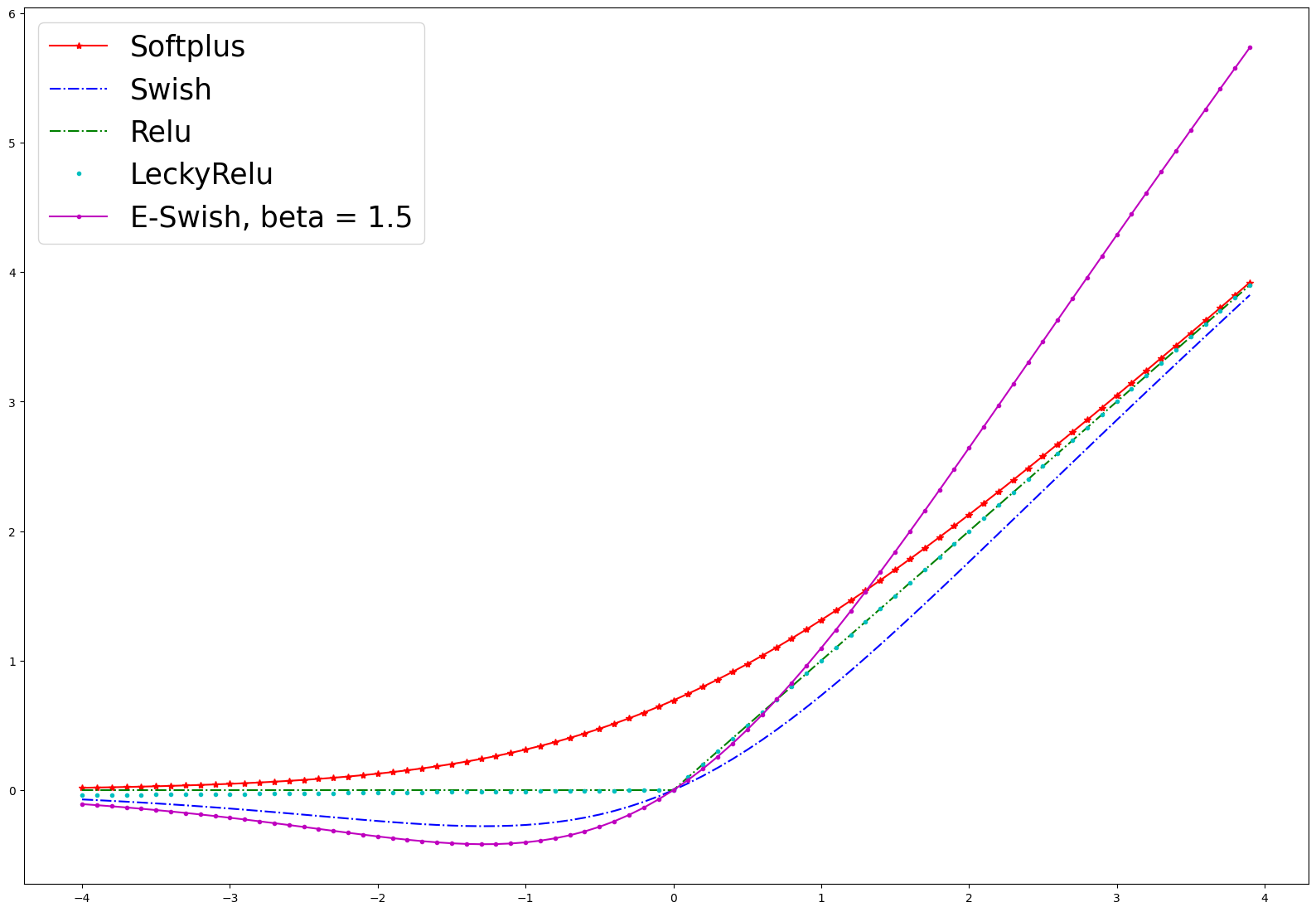
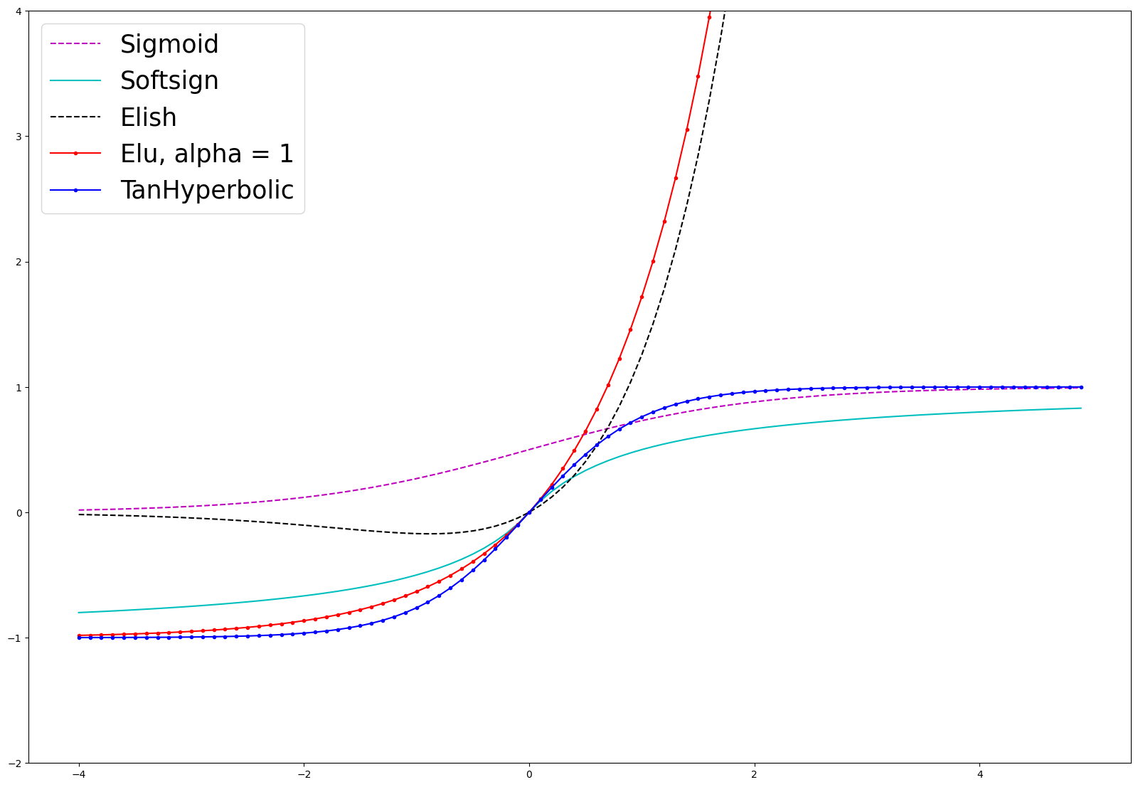
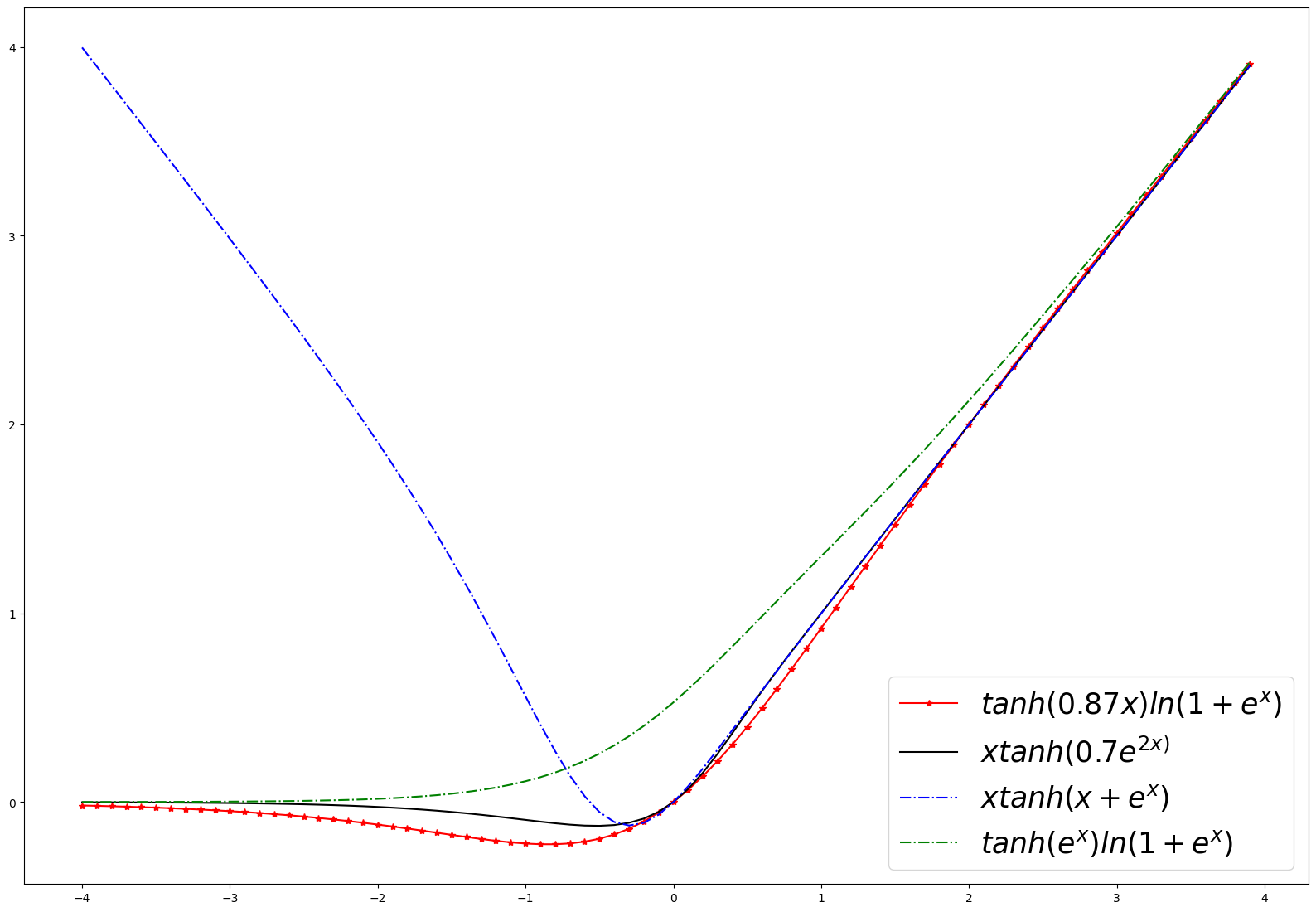
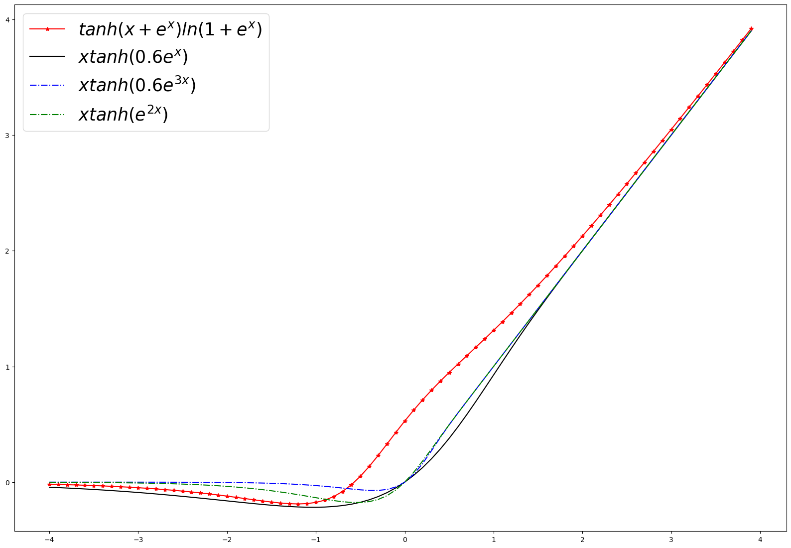
We give a brief idea of a few most widely used activation functions. All of these functions, along with some members of TanhSoft family, are given in Figure 1.

• Sigmoid:- Sigmoid activation function, which is also known as logistic function, used in binary classification problem in outcome layers and it produces outputs based on probability. Sigmoid is a smooth, bounded, non-linear and differentiable function range in $(0,1)$. Sigmoid suffers from vanishing gradient problem. Sigmoid is defined as

  $$\sigma(x)=\frac{1}{1+e^{-x}}$$ (2)

• Hyperbolic Tangent Function:- Hyperbolic Tangent Function, tanh, is a smooth, non-linear and differentiable function in the range $(-1,1)$ defined as

  $$\tanh(x)=\frac{e^{x}-e^{-x}}{e^{x}+e^{-x}}.$$ (3)

  It is used in recurrent neural networks, natural language processing[12] and speech processing tasks but also suffers from vanishing gradient problem.

• Rectified Linear Unit (ReLU):- The rectified linear unit (ReLU) activation function was first introduced by Nair and Hinton in 2010 [REF]. At present, It is one of the most widely used activation function. ReLU is a kind of linear function, and it is identity in the positive axis while $0$ in the negative axis. One of the best property about ReLU is, it learns really fast. ReLU suffers from vanishing gradient problem. Also, in some situation, it has been observed that up-to 50$\%$ of neurons are dead because of 0 value in the negative axis. ReLU([4], [3], [2]) is defined as

  $$f(x)=\max(0,x).$$ (4)

• Leaky Rectified Linear Unit:- Leaky Rectified Linear Unit(Leaky ReLU) was proposed by Mass et al. on 2013[6]. Leaky ReLU has introduced an non-zero gradient in the negative axis to overcome the vanishing gradient and dead neuron problems of ReLU. LReLU is defined as

  $$f(x) =\begin{cases}x&x>0\\ 0.01.x&x\leq 0\end{cases}$$ (5)

• Parametric ReLU:- Parametric ReLU(PReLU) is similar to Leaky ReLU where Leaky ReLU has predetermined negative slope where PReLU has a parametric negative slope. PReLU is defined as

  $$f(x) =\begin{cases}x&x>0\\ a.x&x\leq 0\end{cases}$$ (6)

  where $a\leq 1$ and so f(x) is equivalent to max(x,ax).

• Swish:- To construct Swish, researcher from Google brain team uses reinforcement learning based automatic search technique. It was proposed by Ramachandran et al., on 2017[11]. Swish is a non-monotonic, smooth function which is bounded below and unbounded above. Swish is defined as

  $$f(x)=x\sigma(x)=\frac{x}{1+e^{-x}}$$ (7)

• E-swish:- E-Swish [13] is a slight modified version of Swish function, introduced by Alcaide on 2018, defined by

  $$f(x)=\beta x\sigma(x)$$ (8)

  where $\beta$ is a trainable parameter. This function follows all the properties of Swish and can provide better results than Swish as claimed in the paper for some values of $\beta$.

• ELISH:- Exponential Linear Sigmoid SquasHing(ELiSH) was proposed by Barisat et el. [14] on 2018. It is unbounded above, bounded below, non-monotonic, and smooth function defined by

  $$f(x) =\begin{cases}\frac{x}{1+e^{-x}}&x\geq 0\\ \frac{e^{x}-1}{1+e^{-x}}&x<0\end{cases}$$ (9)

• Softsign:- The Softsign function was proposed by Turian et al., 2009 [15]. Softsign is a quadratic polynomial based function. Softsign is used in regression problem [16] as well as speech system [17] and ac hived some promising results. Softsign is defined as

  $$f(x)=\frac{x}{1+|x|}$$ (10)

  where $|x|$ is absolute value of x.
  

• Exponential Linear Units:- Exponential Linear Units(ELU) was proposed by Clevert et al., 2015 [7]. ELU is deifined in such a way so that it overcomes the vanishing gradient problem of ReLU. ELU is a fast learner and it generalises better than ReLU and LReLU. ELU is defined as

  $$f(x) =\begin{cases}x&x>0\\ \alpha(e^{x}-1)&x\leq 0\end{cases}$$ (11)

  where $\alpha$ is a hyper-parameter.

• Softplus:- Softplus was proposed by Dugas et al., 2001 [18, 19]. Softplus is a smooth activation function and has non-zero gradient. Softplus is defined as

  $$\operatorname{Softplus}(x)=ln(1+e^{x})$$ (12)

Figure 1: Plot of various activation functions

3 TanhSoft activation function family

Standard ANN training process involves tuning the weights in the linear part of the network, however there is a merit in the ability to custom design activation functions, to better fit the problem at hand. Here, rather than looking at individual activation functions, we propose a family of functions indexed by four hyper-parameters. We refer to this family as the TanhSoft family as it is created by combining a hyper-parametric versions of the $\tanh$ and the Softplus activation functions. Explicitly, we express it as

$$f(x;\alpha,\beta,\gamma,\delta)=\tanh(\alpha x+\beta e^{\gamma x})\ln(\delta+e^{x}).$$ (13)

Any function in this family can be used as a activation function for hyper-parameter values $-\infty\leq\alpha\leq 1$ , $0\leq\beta<\infty,0<\gamma<\infty$ and $0\leq\delta\leq 1$, though for experimental and practical purpose, we restrict to small ranges of the hyper-parameters ($0\leq\alpha\leq 3,0\leq\beta<2,0<\gamma<4$ and $\delta=0,1$). The interplay between the hyper-parameters $\alpha,\beta$, and $\gamma$ plays a major role for the TanhSoft family and controls the slope of the curve in both positive and negative axes. The hyper-parameter $\delta$ is used as a switch to change the SoftPlus component of TanhSoft to a linear function ($\delta=0$) allowing us to cover a larger class of functions.

Note that $f(x;0,0,\gamma,\delta)$ recovers the zero function and $f(x;0,\beta,0,0)$ becomes the linear function family $\tanh(\beta)x$. For large values of some parameter while fixing the other parameters, the TanhSoft family converges to some known activation functions pointwise. For example,

$$\lim_{\gamma\to\infty}f(x;0,\beta,\gamma,0)=\operatorname{ReLU}(x)\quad\forall x\in\mathbb{R}\text{ for any fixed }\beta>0.$$

With the similar hyper-parametric settings except for very small negative values of $\alpha$, $f(x;\alpha,\beta,\gamma,0)$ has behaviour similar to the Parametric ReLU activation function. Also,

$$\lim_{\beta\to\infty}f(x;0,\beta,\gamma,1)=\operatorname{Softplus}(x)\quad\forall x\in\mathbb{R}\text{ for any fixed }\gamma>0.$$

We remark that the MISH[20] activation function is also obtained from $\tanh$ and Softplus but it is a composition while we use a hyper-parametric product. Worth noting that the author has reported unstable training behaviour for the specific function $f(x;1,0,\gamma,1)$ in [20], however, we failed to find any instability during the training process. Also, in [21] the authors have mentioned the function $f(x;0,1,1,0)$, which arise as an example from the TanhSoft family. In fact, we show that because of the introduction of hyper-parameters, better activation functions of the form $f(x;0,\beta,\gamma,0)$ can be obtained.

Being a product of two smooth functions, TanhSoft is a family of smooth activation functions. As expected, the monotonocity and boundedness of the functions in the family depend on the specific values of the hyper-parameters. The derivative of the TanhSoft family is given by

$$f^{\prime}(x;\alpha,\beta,\gamma,\delta)=\tanh(\alpha x+\beta e^{\gamma x})\frac{e^{x}}{\delta+e^{x}}+(\alpha+\beta\gamma e^{\gamma x})\operatorname{sech}^{2}(\alpha x+\beta e^{\gamma x})\ln(\delta+e^{x}).$$ (14)

A detailed study of the mathematical properties of the TanhSoft family will be presented in a later work. In this work, we focus on providing several examples of activation functions from the family which perform well on many challenging datasets.

4 Search Findings

We have performed an organized search of activation functions within the TanhSoft family by varying the values of hyper-parameters and training and testing them with DenseNet-121[22] and SimpleNet[23] on CIFAR10[24] dataset. Several functions were tested and we select eight functions as example to report their performance. The Top-1 and Top-3 accuracies of these eight functions are given in Table 1. All these functions, either outperformed or give near accuracy as compared to ReLU. Most notably, $f(x;0,0.6,1,0)=x\tanh(0.6e^{x})$ and $f(x;0.87,0,\gamma,1)=\tanh(0.87x)\ln(1+e^{x})$ constantly outperform ReLU even with more complex models. We have given detailed results in Section 5 with more complex models and datasets.

Figure 2: A few novel activation functions from the searches of the TanhSoft family.

Activation Function	Top-1 accuracy on DenseNet-121	Top-3 accuracy on DenseNet-121	Accuracy on SimpleNet Model
$\operatorname{ReLU}(x)=\max(0,x)$	90.73	98.73	91.01
$f(x;0,0.6,1,0)=x\tanh(0.6e^{x})$	91.14	98.86	92.23
$f(x;0.87,0,\gamma,1)=\tanh(0.87x)\ln(1+e^{x})$	90.98	98.80	92.07
$f(x;0,1,2,0)=x\tanh(e^{2x})$	90.84	98.64	91.38
$f(x;0,0.6,3,0)=x\tanh(0.6e^{3x})$	90.60	98.80	91.20
$f(x;0,1,1,1)=\tanh(e^{x})\ln(1+e^{x})$	90.69	98.42	91.35
$f(x;0,0.7,2,0)=x\tanh(0.7e^{2x})$	91.11	98.66	91.98
$f(x;1,1,1,0)=x\tanh(x+e^{x})$	90.78	98.67	89.42
$f(x;1,1,1,1)=\tanh(x+e^{x})\ln(1+e^{x})$	90.43	98.62	91.58

Table 1: Accuracy on CIFAR-10 for eight example functions from the TanhSoft family along with ReLU.

Real-world datasets are noisy or challenging, and it is always difficult to find the best activation function to generalize on random datasets. It is hard to say whether the searched function will generalize successfully and replace ReLU on challenging or noisy datasets. Though there may be merit in having a custom activation function corresponding to the problem at hand, but yet it is beneficial to identify activation functions that generalize to several real world data sets, making it easier to implement. Hence we concentrate on two members from the TanhSoft family and establish their generalizability and usefulness over other conventional activation functions. In particular, we consider the sub-families $f(x;\alpha,0,\gamma,1)$ and $f(x;0,\beta,\gamma,0)$ and call them as TanhSoft-1 and TanhSoft-2. In what follows, we discuss the properties of these subfamilies, experiments with more complex models, and comparison with a few other widely used activation functions.

5 TanhSoft-1 and TanhSoft-2

The functions, TanhSoft-1 and TanhSoft-2 are given as

$$\text{TanhSoft-1}:\qquad f(x;\alpha,0,\gamma,1)=\tanh(\alpha x)\text{Softplus}(x)=\tanh(\alpha x)\ln(1+e^{x}),$$ (15)

$$\text{TanhSoft-2}:\qquad f(x;0,\beta,\gamma,0)=x\tanh(\beta e^{\gamma x}).$$ (16)

The corresponding derivatives (see equation 14) are

$$\text{Derivative \ of \ TanhSoft-1}:\qquad f^{\prime}(x;\alpha,0,\gamma,1)=\tanh(\alpha x)\frac{e^{x}}{(1+e^{x})}+\alpha\operatorname{sech}^{2}(\alpha x)\ln(1+e^{x}),$$ (17)

$$\text{Derivative \ of \ TanhSoft-2}:\qquad f^{\prime}(x;0,\beta,\gamma,0)=\tanh(\beta e^{\gamma x})+\beta\gamma xe^{\gamma x}\operatorname{sech}^{2}(\beta e^{\gamma x}).$$ (18)

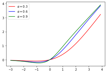
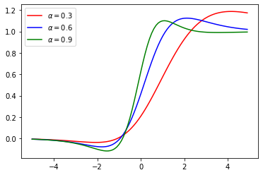
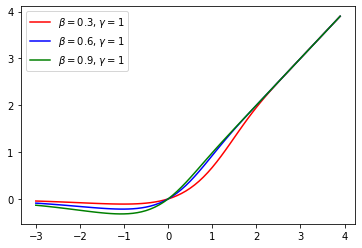
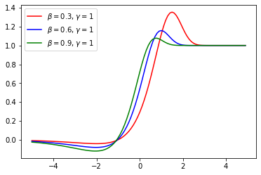
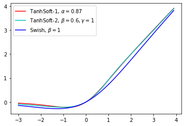
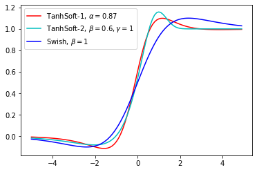
Figure 4 and  6 show the graph for TanhSoft-1 and TanhSoft-2 activation functions for different values of $\alpha$, and $\beta$ and $\gamma$ respectively. If $\alpha=0$, then TanhSoft-1 becomes the zero function. Similarly, for $\beta=0$, TanhSoft-2 is the zero function. Like ReLU and Swish, TanhSoft-1 and TanhSoft-2 are also unbounded above but bounded below. Like Swish, TanhSoft-1 and TanhSoft-2 are both smooth, non-monotonic activation functions. Plots of the first derivative of TanhSoft-1 and TanhSoft-2 are given in Figures 4 and  6 for different values of $\alpha$, and $\beta$ and $\gamma$ respectively. A comparison between TanhSoft-1, TanhSoft-2 and Swish and their first derivatives are given in Figures 8 and 8.

TanhSoft-1 and TanhSoft-2 can be implemented with a single line of code in Keras Library [25] or Tensorflow V2.3.0 [26]. The Keras codes for TanhSoft-1 and TanhSoft-2 are

$$\text{tf.keras.activations.tanh}(\alpha*x)*\text{tf.keras.activations.softplus}(x)\qquad\text{ and, }$$

$$x*\text{tf.keras.activations.tanh}(\beta*\text{tf.keras.activations.exp}(\gamma x))$$

for specific value of $\alpha,\beta$ and $\gamma$ respectively.

Figure 3: TanhSoft-1 Activation for different values of $\alpha$

Figure 4: First order derivative Derivative of TanhSoft-1 Activation for different values of $\alpha$

Figure 5: TanhSoft-2 Activation for different values of $\beta$

Figure 6: First order derivative Derivative of TanhSoft-2 Activation for different values of $\beta$

Figure 7: TanhSoft-1, TanhSoft-2 and Swish

Figure 8: First order derivatives of TanhSoft-1, TanhSoft-2 and Swish

Experiments with TanhSoft-1 and TanhSoft-2

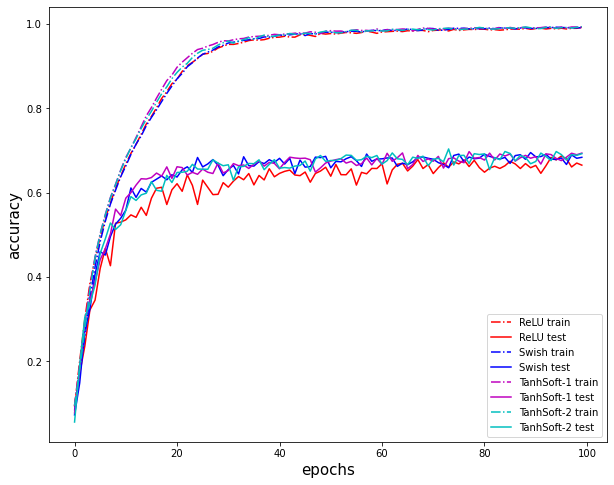
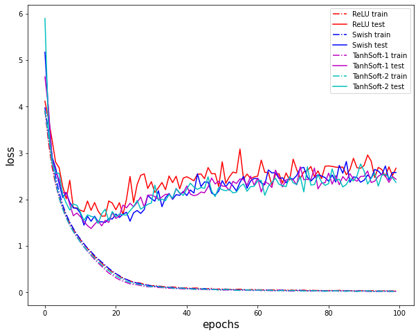
We tested TanhSoft-1 and TanhSoft-2 for different values of hyper-parameters against widely used activation functions on CIFAR and MNIST datasets. In particular, TanhSoft-1 with $\alpha=0.87$, $f(x;0.87,0,\gamma,1)$, and TanhSoft-2 with $\beta=0.6,\gamma=1$, $f(x;0,0.6,1,0)$, produced best results. We observe that $f(x;0.87,0,\gamma,1)$ and $f(x;0,0.6,1,0)$ in most cases beats or performs equally with baseline activation functions, and underperforms marginally on rare occasions. Table 2 gives a comparison with the baseline activation such as ReLU, Leaky ReLU, ELU, Softplus, and Swish. We have tested our activation function in several models, such as Densenet121[22], DenseNet169[22], InceptionNet V3[27], SimpleNet[23], MobileNets[28], WideResNet 28-10[29]. In this next section we will provide details of our experimental framework and results.

Baselines	ReLU	Leaky ReLU	ELU	Swish	Softplus
TanhSoft-1 > Baseline	10	7	11	10	10
TanhSoft-1 = Baseline	1	2	0	1	0
TanhSoft-1 < Baseline	0	2	0	0	1
TanhSoft-2 > Baseline	11	9	11	11	11
TanhSoft-2 = Baseline	0	1	0	0	0
TanhSoft-2 < Baseline	0	1	0	0	0

Table 2: Baseline table of TanhSoft-1 and TanhSoft-2 for Top-1 Accurecy

MNIST

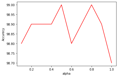
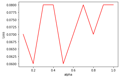
MNIST [30] database contains image data of handwritten digits from 0 to 9. The dataset contains 60k training and 10k testing $28\times 28$ grey-scale images. We run a custom 5-layer CNN architecture on MNIST dataset with different activation functions and results are reported in Table 3. We have reported accuracy and loss for TanhSoft-1 for different values of $\alpha$ in Figures 12 and 12.

Activation Function	5-fold Accuracy on MNIST data
TanhSoft-1($\alpha=0.87$)	99.0 ($\pm$ 0.05)
TanhSoft-2($\beta=0.6,\gamma=1$)	99.1 ($\pm$ 0.05)
ReLU	99.0 ($\pm$ 0.06)
Swish	98.9 ($\pm$ 0.08)
Leaky ReLU($\alpha$ = 0.01)	99.0 ($\pm$ 0.1)
ELU	98.9($\pm$ 0.06)
Softplus	98.9($\pm$ 0.06)

Table 3: Experimental Results with MNIST Dataset

Figure 9: Accuracy with TanhSoft-1 Activation function in MNIST dataset for different values for $\alpha$

Figure 10: Loss with TanhSoft-1 Activation function in MNIST dataset for different values of $\alpha$

CIFAR

The CIFAR [24] dataset consists of $32\times 32$ colored images, consists of 60k images and divided into 50k training and 10k test images. There are two type of CIFAR dataset such as CIFAR10 and CIFAR100. CIFAR10 dataset has 10 classes with 6000 images per class while for CIFAR100 has 100 classes with 600 images per class. We have reported the results of TanhSoft-1 and TanhSoft-1 for $\alpha=0.87$ and $\beta=0.6,\gamma=1$ respectively along with ReLU, Leaky ReLu, ELU, Softplus and Swish in the CIFAR10 dataset with DenseNet121, DenseNet169, InceptionNet V3 and SimpleNet while for CIFAR100 dataset results have been reported with DenseNet121, DenseNet169, InceptionNet V3, MobileNet[28], WideResNet[29] and SimpleNet. We have trained with Adam optimizer[31] with 100 epochs for DenseNet121, DenseNet169, InceptionNet V3, MobileNet, WideResNet and 200 epochs for SimpleNet. We used weight decay $5\times 10^{-4}$ in SimpleNet model. Weight decay has been decided according to[32].  Table 5, 6 contains results for CIFAR10 data while  Table 7, 8 contains results for CIFAR100 data.  Table 4 contains results for accuracy and Loss on CIFAR10 dataset with SimpleNet Model and TanhSoft-2 activation function for different values of $\beta$ and $\gamma=1$

$\beta$	0.1	0.2	0.3	0.4	0.5	0.6	0.7	0.8	0.9	1.0
Accuracy	91.05	91.60	92.01	91.75	91.77	92.23	91.79	91.61	92.05	91.87
Loss	0.5103	0.4631	0.4428	0.4659	0.4480	0.4204	0.4606	0.4688	0.4511	0.4578

Table 4: Accuracy and Loss On CIFAR10 dataset with SimpleNet Model and TanhSoft-2 activation function for different values of $\beta$ and $\gamma=1$

Activation Function	DenseNet 121 Model Top-1 Accuracy	DenseNet 121 Model Top-3 Accuracy	DenseNet 169 Model Top-1 Accuracy	DenseNet 169 Model Top-3 Accuracy
TanhSoft-1($\alpha=0.87$)	90.98	98.80	91.05	98.75
TanhSoft-2($\beta=0.6,\gamma=1$)	91.14	98.86	91.10	98.78
ReLU	90.73	98.73	90.64	98.79
Leaky ReLU($\alpha$ = 0.01)	90.77	98.80	90.61	98.78
ELU	90.49	98.61	90.40	98.65
Swish	90.77	98.80	90.38	98.68
Softplus	90.45	98.65	90.51	98.69

Table 5: Experimental Results with CIFAR10 Dataset with DenseNet-121 and DenseNet-169

Activation Function	SimpleNet Top-1 Accuracy	Inception-Net Model V3 Top-1 Accuracy	Inception Model V3 Top-3 Accuracy
TanhSoft-1($\alpha=0.87$)	92.07	91.93	98.84
TanhSoft-2($\beta=0.6,\gamma=1$)	92.23	91.99	98.85
ReLU	91.01	91.29	98.80
Leaky ReLU($\alpha$ = 0.01)	91.05	91.84	98.93
ELU	91.19	91.01	98.79
Swish	91.59	91.26	98.75
Softplus	91.42	91.79	98.84

Table 6: Experimental Results with CIFAR10 Dataset with SimpleNet and Inception V3

Figure 11: Train and Test accuracy on CIFAR100 dataset with WideResNet 28-10 model

Figure 12: Train and Test loss on CIFAR100 dataset with WideResNet 28-10 model

Activation Function	DenseNet 121 Model Top-1 Accuracy	DenseNet 121 Model Top-3 Accuracy	DenseNet 169 Model Top-1 Accuracy	DenseNet 169 Model Top-3 Accuracy	SimpleNet Top-1 Accuracy
TanhSoft-1($\alpha=0.87$)	66.99	83.76	65.37	82.42	65.20
TanhSoft-2($\beta=0.6,\gamma=1$)	67.18	84.01	64.99	82.09	65.01
ReLU	66.40	83.11	64.15	81.69	62.63
Leaky ReLU($\alpha$ = 0.01)	67.18	83.37	63.40	81.16	62.58
ELU	66.52	83.42	64.23	81.45	63.74
Swish	66.99	83.76	64.95	82.06	64.90
Softplus	65.93	83.50	64.95	82.05	62.39

Table 7: Experimental Results with CIFAR100 Dataset with DenseNet and SimpleNet models

Activation Function	MobileNet Top-1 Accuracy	MobileNet Top-3 Accuracy	Inception V3 Top-1 Accuracy	Inception V3 Top-3 Accuracy	WideResNet 28-10 Top-1 Accuracy
TanhSoft-1($\alpha=0.87$)	57.56	76.57	69.19	84.63	69.40
TanhSoft-2($\beta=0.6$)	57.56	76.57	69.28	85.91	69.41
ReLU	56.87	76.33	69.09	85.41	66.54
Leaky ReLU($\alpha$ = 0.01)	57.78	77.32	69.19	85.24	69.23
ELU	57.19	76.03	68.32	85.30	64.48
Swish	55.40	74.81	67.61	83.59	68.45
SoftPlus	57.53	76.48	69.24	85.15	61.53

Table 8: Experimental Results with CIFAR100 Dataset with MobileNet, Inception V3 and WideResNet 28-10

6 Conclusion

In this study, we have explored a new novel hyper-parameter family of activation functions, TanhSoft, defined mathematically as $\tanh{(\alpha x+\beta e^{\gamma x})}\ln(\delta+e^{x})$ where $\alpha$, $\beta$, $\gamma$ and $\delta$ are tunable hyper-parameters. We have shown that in the different complex models, TanhSoft outperforms in the MNIST, Cipher10, and CIFAR100 datasets compared to ReLU, Leaky ReLU, Swish, ELU, and Softplus so that TanhSoft can be a good choice to replace the ReLU, Swish, and other widely used activation functions. Future work can be, applying the proposed novel activation function to more challenging datasets such as ImageNet & COCO and try on different other models to achieve State-of-the-Art results.

References

- [1] Chigozie Nwankpa, Winifred Ijomah, Anthony Gachagan, and Stephen Marshall. Activation functions: Comparison of trends in practice and research for deep learning, 2018.
- [2] Vinod Nair and Geoffrey E. Hinton. Rectified linear units improve restricted boltzmann machines. In Johannes Fürnkranz and Thorsten Joachims, editors, Proceedings of the 27th International Conference on Machine Learning (ICML-10), June 21-24, 2010, Haifa, Israel, pages 807–814. Omnipress, 2010.
- [3] Kevin Jarrett, Koray Kavukcuoglu, Marc’Aurelio Ranzato, and Yann LeCun. What is the best multi-stage architecture for object recognition? In IEEE 12th International Conference on Computer Vision, ICCV 2009, Kyoto, Japan, September 27 - October 4, 2009, pages 2146–2153. IEEE Computer Society, 2009.
- [4] Richard Hahnloser, Rahul Sarpeshkar, Misha Mahowald, Rodney Douglas, and H. Seung. Digital selection and analogue amplification coexist in a cortex-inspired silicon circuit. Nature, 405:947–51, 07 2000.
- [5] Yuan Zhou, Dandan Li, Shuwei Huo, and Sun-Yuan Kung. Soft-root-sign activation function, 2020.
- [6] Andrew L. Maas, Awni Y. Hannun, and Andrew Y. Ng. Rectifier nonlinearities improve neural network acoustic models. In in ICML Workshop on Deep Learning for Audio, Speech and Language Processing, 2013.
- [7] Djork-Arné Clevert, Thomas Unterthiner, and Sepp Hochreiter. Fast and accurate deep network learning by exponential linear units (elus), 2015.
- [8] Kaiming He, Xiangyu Zhang, Shaoqing Ren, and Jian Sun. Delving deep into rectifiers: Surpassing human-level performance on imagenet classification, 2015.
- [9] Bing Xu, Naiyan Wang, Tianqi Chen, and Mu Li. Empirical evaluation of rectified activations in convolutional network, 2015.
- [10] Brad Carlile, Guy Delamarter, Paul Kinney, Akiko Marti, and Brian Whitney. Improving deep learning by inverse square root linear units (isrlus), 2017.
- [11] Prajit Ramachandran, Barret Zoph, and Quoc V. Le. Searching for activation functions, 2017.
- [12] Yann N. Dauphin, Angela Fan, Michael Auli, and David Grangier. Language modeling with gated convolutional networks, 2016.
- [13] Eric Alcaide. E-swish: Adjusting activations to different network depths, 2018.
- [14] Mina Basirat and Peter M. Roth. The quest for the golden activation function, 2018.
- [15] Joseph Turian, James Bergstra, and Yoshua Bengio. Quadratic features and deep architectures for chunking. In Proceedings of Human Language Technologies: The 2009 Annual Conference of the North American Chapter of the Association for Computational Linguistics, Companion Volume: Short Papers, pages 245–248, Boulder, Colorado, June 2009. Association for Computational Linguistics.
- [16] Phong Le and Willem Zuidema. Compositional distributional semantics with long short term memory, 2015.
- [17] Wei Ping, Kainan Peng, Andrew Gibiansky, Sercan O. Arik, Ajay Kannan, Sharan Narang, Jonathan Raiman, and John Miller. Deep voice 3: Scaling text-to-speech with convolutional sequence learning, 2017.
- [18] Hao Zheng, Zhanlei Yang, Wenju Liu, Jizhong Liang, and Yanpeng Li. Improving deep neural networks using softplus units. In 2015 International Joint Conference on Neural Networks (IJCNN), pages 1–4, 2015.
- [19] Charles Dugas, Yoshua Bengio, François Bélisle, Claude Nadeau, and René Garcia. Incorporating second-order functional knowledge for better option pricing. In Proceedings of the 13th International Conference on Neural Information Processing Systems, NIPS’00, page 451–457, Cambridge, MA, USA, 2000. MIT Press.
- [20] Diganta Misra. Mish: A self regularized non-monotonic activation function, 2019.
- [21] Xinyu Liu and Xiaoguang Di. Tanhexp: A smooth activation function with high convergence speed for lightweight neural networks, 2020.
- [22] Gao Huang, Zhuang Liu, Laurens van der Maaten, and Kilian Q. Weinberger. Densely connected convolutional networks, 2016.
- [23] Seyyed Hossein Hasanpour, Mohammad Rouhani, Mohsen Fayyaz, and Mohammad Sabokrou. Lets keep it simple, using simple architectures to outperform deeper and more complex architectures, 2016.
- [24] Alex Krizhevsky. Learning multiple layers of features from tiny images. Technical report, 2009.
- [25] François Chollet. Keras. https://github.com/fchollet/keras, 2015.
- [26] Martín Abadi, Ashish Agarwal, Paul Barham, Eugene Brevdo, Zhifeng Chen, Craig Citro, Greg S. Corrado, Andy Davis, Jeffrey Dean, Matthieu Devin, Sanjay Ghemawat, Ian Goodfellow, Andrew Harp, Geoffrey Irving, Michael Isard, Yangqing Jia, Rafal Jozefowicz, Lukasz Kaiser, Manjunath Kudlur, Josh Levenberg, Dandelion Mané, Rajat Monga, Sherry Moore, Derek Murray, Chris Olah, Mike Schuster, Jonathon Shlens, Benoit Steiner, Ilya Sutskever, Kunal Talwar, Paul Tucker, Vincent Vanhoucke, Vijay Vasudevan, Fernanda Viégas, Oriol Vinyals, Pete Warden, Martin Wattenberg, Martin Wicke, Yuan Yu, and Xiaoqiang Zheng. TensorFlow: Large-scale machine learning on heterogeneous systems, 2015. Software available from tensorflow.org.
- [27] Christian Szegedy, Vincent Vanhoucke, Sergey Ioffe, Jonathon Shlens, and Zbigniew Wojna. Rethinking the inception architecture for computer vision, 2015.
- [28] Andrew G. Howard, Menglong Zhu, Bo Chen, Dmitry Kalenichenko, Weijun Wang, Tobias Weyand, Marco Andreetto, and Hartwig Adam. Mobilenets: Efficient convolutional neural networks for mobile vision applications, 2017.
- [29] Sergey Zagoruyko and Nikos Komodakis. Wide residual networks, 2016.
- [30] Yann LeCun, Corinna Cortes, and CJ Burges. Mnist handwritten digit database. ATT Labs [Online]. Available: http://yann.lecun.com/exdb/mnist, 2, 2010.
- [31] Diederik P. Kingma and Jimmy Ba. Adam: A method for stochastic optimization. In Yoshua Bengio and Yann LeCun, editors, 3rd International Conference on Learning Representations, ICLR 2015, San Diego, CA, USA, May 7-9, 2015, Conference Track Proceedings, 2015.
- [32] Xavier Glorot and Yoshua Bengio. Understanding the difficulty of training deep feedforward neural networks. In In Proceedings of the International Conference on Artificial Intelligence and Statistics (AISTATS’10). Society for Artificial Intelligence and Statistics, 2010.