Referenced Thermodynamic Integration for Bayesian Model Selection: Application to COVID-19 Model Selection

Abstract

Model selection is a fundamental part of the applied Bayesian statistical methodology. Metrics such as the Akaike Information Criterion are commonly used in practice to select models but do not incorporate the uncertainty of the models’ parameters and can give misleading choices. One approach that uses the full posterior distribution is to compute the ratio of two models’ normalising constants, known as the Bayes factor. Often in realistic problems, this involves the integration of analytically intractable, high-dimensional distributions, and therefore requires the use of stochastic methods such as thermodynamic integration (TI). In this paper we apply a variation of the TI method, referred to as referenced TI, which computes a single model’s normalising constant in an efficient way by using a judiciously chosen reference density. The advantages of the approach and theoretical considerations are set out, along with explicit pedagogical 1 and 2D examples. Benchmarking is presented with comparable methods and we find favourable convergence performance. The approach is shown to be useful in practice when applied to a real problem — to perform model selection for a semi-mechanistic hierarchical Bayesian model of COVID-19 transmission in South Korea involving the integration of a 200D density.

1 Introduction

Bayesian computation has been in the limelight in recent months. Modern techniques of statistical machine learning, in particular those based on stochastic inference, have been central to current epidemiological models [1, 2], with statistical inference underpinning estimates of pathogen transmission being used to make informed public health policy. With advances in both computing power and availability of data, it is possible to build more complex, reliable and accurate models, while the recent increased focus on epidemiological models emphasises a need for synthesis with rigorous statistical methods. This synthesis is required to robustly estimate necessary parameters, quantify uncertainty in predictions, and to test hypotheses [3].

In practice the decision to choose a model is often based on heuristics, relying on the knowledge and experience of the modeller, rather than through a systematic selection process [4, 5]. A number of model selection methods are available, but those methods often come with a trade-off between accuracy and computational complexity. For example, widely used in epidemiology Akaike Information Criterion (AIC) or Bayesian Information Criterion (BIC) are easy to compute, but come with certain limitations [3]. Specifically, they do not take into account the parameters’ uncertainty or the prior probabilities, and might favour excessively complex models.

The ratio of two normalising constants — the Bayes factor (BF) — is a popular and general method used for model selection in the Bayesian setting [6]. This approach integrates out the parameters of the model to find the probability of the getting the data from a given model hypothesis. But in general a normalising constant cannot be computed analytically or through direct quadrature methods, due to the difficulty of integrating arbitrary high-dimensional distributions. Typically approximations are applied such as Laplace’s method, variational approximations, or probabilistic algorithms such as bridge sampling [7, 8], stochastic density of states based methods [9, 10] or thermodynamic integration [11, 12, 13, 14].

Thermodynamic integration (TI) provides a useful way estimate the log ratio of the normalising constants of two densities. Instead of marginalising the densities explicitly in terms of the high-dimensional integrals, by using TI we only need to evaluate a 1-dimensional integral, where the integrand can easily be sampled with Markov Chain Monte Carlo (MCMC). To see how this works, consider two models with the pair of normalising constants $z_{1}$ and $z_{2}$,

$$z_{i}=\int q_{i}(\bm{\theta})d\bm{\theta}\,,\,\,i\in\{1,2\}\,,$$ (1)

where $q_{i}$ is a density for model $M_{i}$ with parameters $\bm{\theta}$, that can be normalised to give the model’s Bayesian posterior density

$$p_{i}(\bm{\theta})=\frac{q_{i}(\bm{\theta})}{z_{i}}\,,\,\,i\in\{1,2\}\,.$$

To apply thermodynamic integration we introduce the concept of a path between $q_{1}(\bm{\theta})$ and $q_{2}(\bm{\theta})$, linking the two densities via a series of intermediate ones. This family of densities is denoted $q(\lambda;\bm{\theta})$. An example path in $\lambda$ is shown in Figure 1. Note — we use the symbol $\lambda$ but often the coupling parameter is denoted $\beta$ (or $t$) in reference to a physical thermodynamic integration in inverse temperature (or temperature). In learning terms the temperature represents a Lagrange multiplier regularising the loss, and in many instances the tempering analogy is useful. Here however the approach is a more generic procedure and we prefer to consider it simply as a path integration between two distributions coupled by an arbitrary but common switching parameter $\lambda$.

The parametric density $q(\lambda;\bm{\theta})$, linking $q_{1}$ to $q_{2}$ and defining the intermediate densities, can be chosen to have an optimal or in some way convenient path, but a common choice is the geometric one

$$q(\lambda;\bm{\theta})=q_{2}^{\lambda}(\bm{\theta})q_{1}^{1-\lambda}(\bm{\theta})\,,\,\,\lambda\in[0,1]\,.$$

The important point to note is that for $\lambda=0$, $q(\lambda;\bm{\theta})$ returns the first density $q(0;\bm{\theta})=q_{1}(\bm{\theta})$, for $\lambda=1$ it gives $q(1;\bm{\theta})=q_{2}(\bm{\theta})$, and for in-between $\lambda$ values a log-linear mixture of the endpoint densities. Just as we have defined a family of densities, there is an associated normalising constant for any point along the path, that for any value of $\lambda$ is given by

$$z(\lambda)=\int_{\Omega(\lambda)}q(\lambda;\bm{\theta})d\bm{\theta}\,.$$

A further small but important point to avoid complications is to have densities that have common support, for example ${\Omega(1)}={\Omega(0)}$. Hereafter support is denoted $\Omega$.

Having set up the definitions of $q(\lambda;\bm{\theta})$ and $z(\lambda)$, the TI expression can be derived, to compute the log ratio of $z_{1}=z(0)$ and $z_{2}=z(1)$, while avoiding explicit integrals over the models’ parameters $\bm{\theta}$. By the fundamental theorem of calculus, assuming that the order of $\partial_{\lambda}$ and $\int d\bm{\theta}$ integral can be exchanged, and by the rules of differentiating logarithms we get:

$$\text{log}\,\frac{z_{2}}{z_{1}} = \int_{0}^{1}\partial_{\lambda}\text{log\,}z(\lambda)\,d\lambda$$ (2)

$$= \int_{0}^{1}\frac{1}{z(\lambda)}\partial_{\lambda}z(\lambda)\,d\lambda$$

$$= \int_{0}^{1}\frac{1}{z(\lambda)}\partial_{\lambda}\int_{\Omega}q(\lambda;\bm{\theta})\,d\bm{\theta}\,d\lambda$$

$$= \int_{0}^{1}\frac{1}{z(\lambda)}\int_{\Omega}\left(\partial_{\lambda}\text{log}\,q(\lambda;\bm{\theta})\right)q(\lambda;\bm{\theta})\,d\bm{\theta}\,d\lambda$$

$$= \int_{0}^{1}\mathbb{E}_{p(\lambda;\bm{\theta})}\left[\partial_{\lambda}\text{log\,}q(\lambda;\bm{\theta})\right]\,d\lambda$$

$$= \int_{0}^{1}\mathbb{E}_{p(\lambda;\bm{\theta})}\left[\text{log\,}\frac{q_{2}(\bm{\theta})}{q_{1}(\bm{\theta})}\right]\,d\lambda$$

$$= \int_{0}^{1}\mathbb{E}_{q(\lambda;\bm{\theta})}\left[\text{log\,}\frac{q_{2}(\bm{\theta})}{q_{1}(\bm{\theta})}\right]\,d\lambda\,.$$

The notation $\mathbb{E}_{q(\lambda;\theta)}$ is for an expectation with respect to the sampling distribution $q(\lambda;\theta)$. The final line in the expression summarises the usefulness of TI—instead of having to work with the complicated high-dimensional integrals of Equation 1 to find the log-Bayes factor $\text{log}\,\frac{z_{2}}{z_{1}}$, we only need consider a 1-dimensional integral of an expectation, and the expectation can be readily produced by MCMC.

Here we set out in detail some variations on the TI theme that we have found to be useful in practice, in particular with regard to evaluating evidence for epidemiological models. The variation is to work primarily in terms of appropriately chosen reference normalising constants. The approach of using exactly integrate-able references has provided us with a particularly efficient method of selection between different hierarchical Bayesian models models, and we hope the approach will be useful to others working on similar problems, for example in phylogenetic model selection where TI is already a popular established method [15, 14].

In the following, we begin with introducing the reference density, then go on to illustrate different practical choices of a reference normalising constant, along with theoretical and practical considerations. Next, the mechanics of applying the method are set out for two simple pedagogical examples. Performance benchmarks are discussed for a well-known problem in the statistical literature [16], which shows the method performs favourably in terms of accuracy and the number of iterations to convergence. Finally the technique is applied to a hierarchical Bayesian time-series model describing the COVID-19 epidemic in South Korea. In the COVID-19 infections model we show how the approach may be used to select technical parameters that specify the reproduction number ($R_{t}$) model, such as the autoregression window size and AR($k$) lag, as well epidemiologically meaningful parameters such as the serial interval distribution time for generating infections.

2 Referenced-TI

An efficient approach to compute Bayes factors, or more generally to marginalise a given density for any application, is to introduce a reference as

$$z = z_{\text{ref}}\,\frac{z}{z_{\text{ref}}}$$ (3)

$$= z_{\text{ref}}\,\text{exp}\int_{0}^{1}\mathbb{E}_{q(\lambda;\bm{\theta})}\left[\text{log\,}\frac{q(\bm{\theta})}{q_{\text{ref}}(\bm{\theta})}\right]\,d\lambda\,.$$

To clarify notation, $z$ is the normalising constant of interest with density $q$, $z_{\text{ref}}$ is a reference normalising constant with associated density $q_{\text{ref}}$. The second line replaces the ratio $z/z_{\text{ref}}$ with a thermodynamic integral as per the identity derived in Equation 2.

The introduction of a reference naturally facilitates the marginalisation of a single density, rather than requiring pairwise model comparisons by direct application of Equation 2. This is useful when comparing multiple models as $n>\binom{n}{2}$ for $n\geq 3$. Another motivation to reference the TI is the MCMC computational efficiency of converging the TI expectation. In Equation 3, with judicious choice of $q_{\text{ref}}$, the reference normalising constant $z_{\text{ref}}$ can be evaluated analytically and account for most of $z$. In this case $\text{log\,}\frac{q(\bm{\theta})}{q_{\text{ref}}(\bm{\theta})}$ tends to have a small expectation and variance and converges quickly.

The idea of using an exactly solvable reference, to aid in the solution of an otherwise intractable problem, is a recurrent and perennial theme in the computational and mathematical sciences in general [17, 18, 19, 20], and variations on this approach have been used to compute normalising constants in various guises in the statistical literature [21, 13, 22, 14, 15, 23, 24, 25, 26]. For example, in the generalised stepping stone method a reference is introduced to speed up convergence of the importance sampling at each temperature rung [25, 26]. In the work of Lefebvre et al. [24] a theoretical discussion has been presented that shows the error budget of thermodynamic integration depends on the J-divergence of the densities being marginalised. Noting this, Cameron and Pettitt [23] illustrate in their work on recursive pathways to marginal likelihood estimation, that a "data driven" auxiliary density reduces standard errors for a 2D banana-shaped likelihood posterior. While, in the power posteriors (PP) approach, the reference in Equation 3 is the prior distribution of $q$ and thus $z_{\text{ref}}=1$ [21]. This approach is elegant as the reference need not be chosen — it is simply the prior — however the downside of the simplicity is that for poorly chosen or uninformative priors, the thermodynamic integral will be slow to converge and susceptible to instability. In particular for complex hierarchical models with weakly informative priors this is found to be an issue.

The reference density in Equation 3 can be chosen at convenience, but the main desirable features are that it should be easily formed without special consideration or adjustments, similar to the power posteriors method, and that $z_{\text{ref}}$ should be analytically integratable and account for as much of $z$ as possible. Such a choice of $z_{\text{ref}}$ ensures the part with expensive sampling is small and convergence is fast. An obvious choice in this regard is the Laplace-type reference, where the log density is approximated with a second-order one, for example a multivariate Gaussian. For densities with a single concentration, Laplace-type approximations are ubiquitous, and an excellent natural choice for many problems. In the following section we consider three approaches that can be used to formulate a reference normalising constant $z_{\text{ref}}$ from a second-order log density (though more generally other tractable references are possible). In each referenced TI scenario, we note that even if the reference approximation is poor, the estimate of the normalising constant based on Equation 3 remains asymptotically exact—only the speed of convergence may be reduced (subject to the assumptions of matching support of endpoint densities).

2.1 Taylor Expansion at the Mode Laplace Reference

The most straightforward way to generate a reference density is to Taylor expand $\text{log}\,q(\bm{\theta})$ to second order about a mode. Noting there is no linear term, we see the reference density is

$$q_{\text{ref}}(\bm{\theta}) = \text{exp}\left(\text{log}\,q(\bm{\theta}_{0})+\frac{1}{2}(\bm{\theta}-\bm{\theta}_{0})^{\text{T}}\mathbf{H}\,(\bm{\theta}-\bm{\theta}_{0})\right)\,,$$ (4)

where $\mathbf{H}$ is the hessian matrix and $\bm{\theta}_{0}$ is the vector of mode parameters. The associated normalising constant is

$$z_{\text{ref}} = \int_{-\infty}^{\infty}q_{\text{ref}}(\bm{\theta})d\bm{\theta}\,$$ (5)

$$= \text{$\int_{-\infty}^{\infty}$exp}\left(\text{log}\,q(\bm{\theta}_{0})+\frac{1}{2}\left(\bm{\theta}-\bm{\theta}_{0}\right)^{\text{T}}\mathbf{H}\left(\mathbf{\bm{\theta}}-\bm{\theta}_{0}\right)\right)d\bm{\theta}$$

$$= \text{q($\bm{\theta}_{0}$)$\int_{-\infty}^{\infty}$exp}\left(\frac{1}{2}\left(\bm{\theta}-\bm{\theta}_{0}\right)^{\text{T}}\mathbf{H}\left(\mathbf{\bm{\theta}}-\bm{\theta}_{0}\right)\right)d\bm{\theta}$$

$$= q(\bm{\theta}_{0})\sqrt{\text{det}(2\pi\mathbf{H}^{-1})}\,.$$

The Taylor expansion method at the mode with analytic or finite difference gradients tends to produce a reference density that works well in the neighbourhood of $\bm{\theta}_{0}$ but can be less suitable if density is asymmetric, has long or short tails, or if the derivatives at the mode are poorly approximated for example due to cusps or conversely very flat curvature at the mode. In many instances a more reliable choice of reference can found by using MCMC samples from the whole posterior density.

2.2 Sampled Covariance Laplace Reference

The second straightforward but often more robust approach is to form a reference density by drawing samples from the true density $q(\bm{\theta})$, to estimate the mean parameters $\hat{\bm{\theta}}$ and covariance matrix $\hat{\bm{\Sigma}}$, such that

$$q_{\text{ref}}(\bm{\theta}) = q(\hat{\bm{\theta}})\,\text{exp}\left(-\frac{1}{2}(\bm{\theta}-\hat{\bm{\theta}})^{\text{T}}\bm{\hat{\Sigma}}^{-1}\,(\bm{\theta}-\hat{\bm{\theta}})\right)\,.$$ (6)

The reference normalising constant is $z_{\text{ref}}=q(\hat{\bm{\theta}})\sqrt{\text{det}(2\pi\hat{\bm{\Sigma}})}\,$.

This method of generating a reference is simple and reliable. It requires sampling from the posterior $q(\bm{\theta})$ so is more expensive than derivative methods, but the cost associated with drawing enough samples to generate a sufficiently good reference tends to be quite low. In the primary application discussed later, regarding relatively complex high-dimensional Bayesian hierarchical models, we use this approach to generate a reference density and normalising constant.

The sampled covariance reference is typically a good approach, but it is not in general optimal within the Laplace-type family of approaches — typically another Gaussian reference exists with different parameters that can generate a normalising constant closer to the true one, thus potentially leading to overall faster convergence of the thermodynamic integral to the exact value. Such an optimal reference can be identified variationally.

2.3 Variational Laplace Reference

The conditions to identify an optimal reference normalising constant can be derived by considering a Taylor expansion of the log normalising constant $\text{log}\,z(\lambda)$ about $\lambda=0$:

$$\text{log}\,z(\lambda)\approx\text{log}\,z(0)+\lambda\,\partial_{\lambda}\text{log}\,z(0)+\frac{1}{2}\lambda^{2}\,\partial_{\lambda}^{2}\text{log}\,z(0)\,.$$

The first derivative gives the expectation

$$\text{$\partial_{\lambda}$log\,}z(\lambda)=\mathbb{E}_{q(\lambda;\bm{\theta})}\left[\text{log\,}\frac{q(\bm{\theta})}{q_{\text{ref}}(\bm{\theta})}\right]\,,$$

as per the derivation in Equation 2, and the second derivative is a variance

$$\text{$\partial_{\lambda}^{2}$log\,}z(\lambda) = \frac{\int\left(\text{log}\,\frac{q(\bm{\theta})}{q_{\text{ref}}(\bm{\theta})}\right)^{2}q(\lambda;\bm{\theta})d\bm{\theta}}{\int q(\lambda;\bm{\theta})d\bm{\theta}}-\left(\frac{\int\left(\text{log}\,\frac{q(\bm{\theta})}{q_{\text{ref}}(\bm{\theta})}\right)\,q(\lambda;\bm{\theta})d\bm{\theta}}{\int q(\lambda;\bm{\theta})d\bm{\theta}}\right)^{2}$$

$$= \left\{\mathbb{E}_{q(\lambda;\bm{\theta})}\left[\left(\text{log}\,\frac{q(\bm{\theta})}{q_{\text{ref}}(\bm{\theta})}\right)^{2}\right]-\mathbb{E}_{q(\lambda;\bm{\theta})}\left[\text{log}\,\frac{q(\bm{\theta})}{q_{\text{ref}}(\bm{\theta})}\right]^{2}\right\}$$

$$\geq 0\,.$$

As the curvature of $\text{log}\,z(\lambda)$ is increasing, to first order we see

$$\text{log}\,z(\lambda)\geq\text{log\,$z(0)$+$\lambda\mathbb{E}_{q(0;\bm{\theta})}\left[\text{log}\,\frac{q(\bm{\theta})}{q_{0}(\bm{\theta})}\right]$}\,,$$

and for the specific case of $\lambda=1$,

$$\text{log}\,z\geq\text{log\,$z_{\text{ref}}$+$\mathbb{E}_{q_{\text{ref}}(\bm{\theta})}\left[\text{log}\,\frac{q(\bm{\theta})}{q_{\text{ref}}(\bm{\theta})}\right]$}\,.$$

This inequality establishes bounds that can be maximised with respect to the position ($\bm{\mu}$) and scale ($\bm{S}$) parameters of a reference density such as

$$q_{\text{ref}}(\bm{\mu},\bm{S};\bm{\theta})=q(\bm{\mu})\text{exp}\left(-\frac{1}{2}(\bm{\theta}-\bm{\mu})^{\text{T}}\bm{S}\,(\bm{\theta}-\bm{\mu})\right)\,.$$

Thus the parameters that optimise

$$\underset{\bm{\mu},\bm{S}}{\text{max}}\left\{\text{log}\,z_{\text{ref}}+\mathbb{E}_{q_{\text{ref}}(\bm{\theta})}\left[\text{log}\,\frac{q(\bm{\theta})}{q_{\text{ref}}(\bm{\mu},\bm{S};\bm{\theta})}\right]\right\}\,,$$

provide a reference density that is variationally optimal. We note this is an application of what is known as the Gibbs-Feynman-Bogoliubov inequality from other fields [27, 28, 29], and that finding approximations of this type to the true density is a well-studied problem in machine learning, with well-documented approaches that can be used to determine $q_{\text{ref}}$ variationally [30, 31]. In itself the existence of a variational bound provides no guarantee of being a good approximation to the true normalising constant, and is thus alone not a satisfactory general approach. However as a point of reference from which to estimate the true normalising constant, it provides a first-order optimal density within the family of trial reference functions considered, therefore improving convergence to the MCMC normalising constant in referenced TI.

2.4 Multi-reference TI

Having set out three approaches to find a single reference for the TI expression in Equation 3, a natural generalisation is the telescopic expansion

$$z = z_{0}\,{\prod_{i=0}^{n-1}}\frac{z_{i+1}}{z_{i}}\frac{z}{z_{n}}$$ (7)

$$= z_{0}\,\text{exp}\left(\int_{0}^{1}{\sum_{i=0}^{n-1}}\mathbb{E}_{q_{i}(\lambda;\bm{\theta})}\left[\text{log\,}\frac{q_{i+1}(\bm{\theta})}{q_{i}(\bm{\theta})}\right]+\mathbb{E}_{q_{n}(\lambda;\bm{\theta})}\left[\text{log\,}\frac{q(\bm{\theta})}{q_{n}(\bm{\theta})}\right]\,d\lambda\right)\,.$$

Note, here the analytic reference is denoted $z_{0}$ rather than $z_{\text{ref}}$ to generalise the indexing. In cases where $q_{0}$ differs substantially from $q$, the telescopic generalisation can improve numerical stability. By bridging the endpoints in terms of intermediate density pairs, $\frac{q_{i+1}(\bm{\theta})}{q_{i}(\bm{\theta})}$, we can form a series of lower variance MCMC simulations with favourable convergence properties. A reasonable choice for generating intermediate densities is for the $q_{i^{\text{th}}}$ density to be the $2\left(i+1\right)^{\text{th}}$ order Taylor expansion of $q(\bm{\theta})$.

2.5 Reference Support

If a model has parameters with limits, for example $\theta_{1}\in[0,\infty)$, $\theta_{2}\in(-1,\infty)$ etc., in referenced TI the exact analytic integration for the reference density should be commensurately limited. However, the calculation of arbitrary probability density function orthants, even for well-known analytic functions such as the multivariate Gaussian, is in general a difficult problem. Computing high-dimensional orthants usually requires advanced techniques, the use of approximations, or sampling methods [32, 33, 34, 35, 36, 37]. Fortunately we can simplify our reference density to create a reference with tractable analytic integration for limits by using a diagonal approximation to the sampled covariance or hessian matrix. For example the orthant of a diagonal multivariate Gaussian can be given in terms of the error function [38], leading to the expression

$$z_{\text{ref}} = q(\hat{\bm{\theta}})\sqrt{\text{det}(2\pi\bm{\Sigma}^{\text{diag}})}\prod_{i\in K}\left(1+\text{erf}\left(\frac{\hat{\theta}_{i}-a_{i}}{\sqrt{2\Sigma_{i}^{\text{diag}}}}\right)\right)\,,$$ (8)

where $K$ denotes the set of indices of the parameters with lower limits $a_{i}$. $\Sigma^{\text{diag}}$ is a diagonal covariance matrix, that is one containing only the variance of each of the parameters, without the covariance terms and $\Sigma_{i}^{\text{diag}}$ denotes the $i^{\text{th}}$ element of the diagonal. Restricting our density to a diagonal one is a poorer approximation than using the full covariance matrix. In practice however this has not been particularly detrimental to the convergence of the thermodynamic integral—and again we note that the quality of the reference only affects convergence rather than eventual theoretical Monte Carlo accuracy of the normalising constant. This behaviour is observed in the practical examples later considered, though the distinction between accuracy and convergence and matters of asymptotic consistency using an MCMC estimator with finite iterations are naturally less clear cut.

2.6 Technical Implementation

The referenced TI algorithm was implemented in Python and Stan programming languages. Using Stan enables fast MCMC simulations, using Hamiltonian Monte Carlo (HMC) and No-U-Turn samples (NUTS) algorithm [39, 40], and portability between other statistical languages, such as R or Julia. Additionally it is familiar to many epidemiologists using Bayesian statistics [41]. The code for all examples shown in this paper is available at https://github.com/mrc-ide/referenced-TI. In the examples shown in Section 3, we used 4 chains with 20,000 iterations per chain for the pedagogical examples, and 4 chains with 2,000 iterations for the other applications. In all cases, half of iterations were used for the burn-in. Mixing of the MCMC chains and the sampling convergence was checked in each case, by ensuring that the $\hat{R}$ value was $\leq 1.05$ for each parameter in every model.

In all examples in the remaining part of this paper, the integral given in Equation 2 was discretised to allow computer simulations. Each expectation $\mathbb{E}_{q(\lambda;\theta)}\left[\text{log\,}\frac{q_{1}(\theta)}{q_{0}(\theta)}\right]$ was evaluated at $\lambda=0.0,0.1,0.2,....,0.9,1.0$, unless stated otherwise. To obtain the value of the integral in Equation 2, we interpolated a curve linking the expectations using a cubic spline, which was then integrated numerically. The pseudo-code of the algorithm with sampled covariance Laplace reference is shown in Algorithm 1.

Algorithm 1 Referenced thermodynamic integration algorithm

Input $q$ - un-normalised density, $q_{\text{ref}}$ - un-normalised reference density, $\Lambda$ - set of coupling parameters $\lambda$, $N$ - number of MCMC iterations
      Output $z$ - normalising constant of the density $q$

1:Define un-normalised density $q$ and the reference density $q_{\text{ref}}$

2:Calculate $z_{\text{ref}}$ analytically by using the determinant of the covariance matrix.

3:for $\lambda\in\Lambda$ do

4:     Sample N values $\theta_{n}$ from $q^{\lambda}q_{\text{ref}}^{1-\lambda}$

5:     for $n=1,2,\ldots,N$ do

6:         Calculate $\text{log}\frac{q(\theta_{n})}{q_{\text{ref}}(\theta_{n})}$

7:     end for

8:     Compute the mean, $\mathbb{E}_{\lambda}=\frac{1}{N}\Sigma_{n=1}^{N}\text{log}\frac{q(\theta_{n})}{q_{\text{ref}}(\theta_{n})}$

9:end for

10:Interpolate between the consecutive $\mathbb{E}_{\lambda}$ values to obtain a curve $\partial_{\lambda}\text{log}(z(\lambda))$

11:Integrate $\partial_{\lambda}\text{log}(z(\lambda))$ over $\lambda\in[0,1]$ to get $\text{log}\frac{z}{z_{\text{ref}}}$

12:Calculate $z$ = $z_{\text{ref}}\cdot\text{exp}\{\text{log}\frac{z}{z_{\text{ref}}}\}$

3 Applications

In this section we present an application of the referenced TI algorithm to 1- and 2-dimensional pedagogical examples, a linear regression model, and a model selection task for a model of COVID-19 epidemic in South Korea.

3.1 1D Pedagogical Example

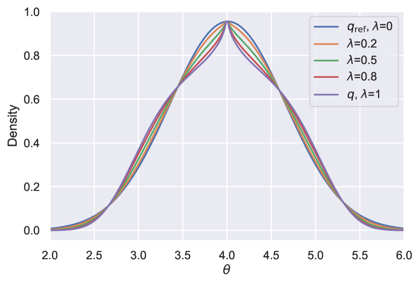
(a)

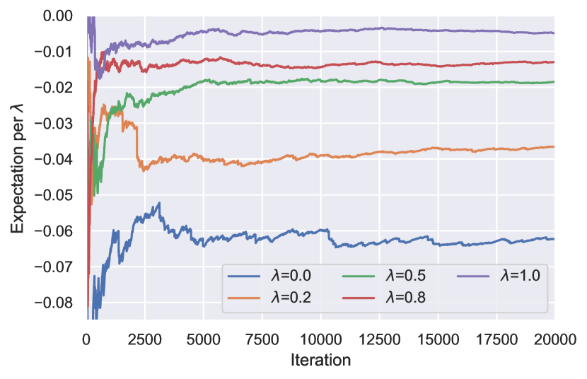
(b)

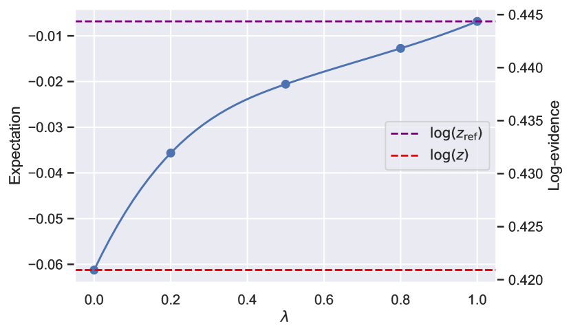
(c)

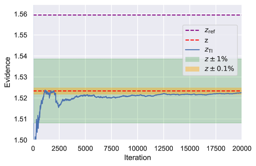
(d)

Figure 1: a) $q^{\lambda}q_{\text{ref}}^{(1-\lambda)}$ for the 1d example density (Equation 9) at selected $\lambda$ values along the path. b) Expectation $\mathbb{E}_{q(\lambda;\bm{\theta})}\left[\text{log\,}\frac{q(\bm{\theta})}{q_{\text{ref}}(\bm{\theta})}\right]$ vs MCMC iteration, shown at each value of $\lambda$ sampled. c) $\lambda$-dependence of the TI contribution to the log-evidence d) Convergence of the evidence $z$, with $1$% convergence after $500$ iterations and $0.1$% after $17,000$ iterations per $\lambda$.

To illustrate the technique consider the 1-dimensional density

$$q(\theta)=\text{exp}\left(-\frac{1}{2}\sqrt{\left|\theta-4\right|}-\frac{1}{2}\left(\theta-4\right)^{4}\right)\,\text{, }\theta\in\mathbb{R},$$ (9)

with normalising constant $z=\int_{-\infty}^{\infty}q(\theta)d\theta$. This density has a cusp — one of the more awkward pathologies of some naturally occurring densities [42, 43] — and it does not have an analytical integral that easily generalises to multiple dimensions, but is otherwise a made-up 1-dimensional example that could be interchanged with an other.

In this instance the Laplace approximation based on the second-order Taylor expansion at the mode will fail due to the cusp, so we can use the more robust covariance sampling method. Sampling from the 1d density $q(\theta)$ we find a variance of $\hat{\sigma}^{2}=0.424$, giving a Gaussian reference density $q_{\text{ref}}(\theta)$ with normalising constant of $z_{\text{ref}}=1.559$. The full normalising constant, $z=z_{\text{ref}}\frac{z}{z_{\text{ref}}}$, is evaluated by Equation 3, by setting up a thermodynamic integration along the sampling path $q^{\lambda}q_{\text{ref}}^{(1-\lambda)}$. The expectation, $\mathbb{E}_{q(\lambda;\bm{\theta})}\left[\text{log\,}\frac{q(\bm{\theta})}{q_{\text{ref}}(\bm{\theta})}\right]$, is evaluated at $5$ points along the coupling parameter path $\lambda={0.0,0.2,0.5,0.8,1.0}$, shown in Figure 1. In this simple example, the integral can be easily evaluated to high accuracy using quadrature [44, 45], giving a value of $1.523$. Referenced thermodynamic integration reproduces this value, with convergence of $z$ shown in Figure 1, converging to $1$% of $z$ with $500$ iterations and $0.1$% within $17,000$ iterations.

This example illustrates notable characteristic features of referenced thermodynamic integration. Here the reference $q_{\text{ref}}(\theta)$ is a good approximation to $q(\theta)$, with $z_{\text{ref}}$ accounting for most ($102$%) of $z$. Consequently $\frac{z}{z_{\text{ref}}}$ is close to 1, and the expectations, $\mathbb{E}_{q(\lambda;\bm{\theta})}\left[\text{log\,}\frac{q(\bm{\theta})}{q_{\text{ref}}(\bm{\theta})}\right]$, evaluated by MCMC for the remaining part of the integral are small. For the same reasons the variance at each $\lambda$ is small, leading to favourable convergence within a small number of iterations. And finally $\mathbb{E}_{q(\lambda;\bm{\theta})}\left[\text{log\,}\frac{q(\bm{\theta})}{q_{\text{ref}}(\bm{\theta})}\right]$ weakly depends on $\lambda$, so there is no need to use a very fine grid of $\lambda$ values or consider optimal paths—satisfactory convergence is easily achieved using a simple geometric path with $4$ $\lambda$ intervals.

3.2 2D Pedagogical Example with Constrained Parameters

As a second example, consider a 2-dimensional un-normalised density with a constrained parameter space:

$$q(\theta_{1},\theta_{2})=\text{exp}\left[-\frac{1}{4}\left[(\theta_{1}+\frac{1}{2})^{2}+(\theta_{1}+\frac{1}{2})^{4}+(\theta_{2}+\frac{1}{2})^{2}+(\theta_{2}+\frac{1}{2})^{4}+\frac{1}{2}\theta_{1}\theta_{2}^{2}\right]\right]\,,$$ (10)

where

$$\theta_{1}\in[0,+\infty)\text{ and }\theta_{2}\in(-\infty,+\infty)\,.$$

A reference density $q_{\text{ref}}(\bm{\theta})$ can be constructed from the Hessian at the mode of $q(\bm{\theta})$. Notice, that because parameter $\theta_{1}$ is constrained to be $\geq 0$, integrating the Gaussian approximations $q_{\text{ref}}(\bm{\theta})$ using the formula given in Equation 5 will give an overestimate. To account for this we use the reference density $q^{\text{diag}}_{\text{ref}}(\bm{\theta})$, based on a diagonal Hessian, that has an exact and easy to calculate orthant. All densities are shown in Figure 2.

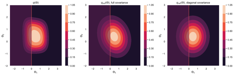
Figure 2: Contour plots of the un-normalised density $q$ and its two reference densities $q_{ref}$, one using a full covariance matrix and another using a diagonal covariance matrix. The red line shows the lower boundary $\theta_{1}=0$ and the shaded $\theta_{1}<0$ region to the left of the line is outside of the support of the density $q$.

To obtain the log-evidence of the model, we calculated the exact value numerically [46, 44], using the full covariance Laplace method as per Equation 6 and using the diagonal covariance with correction added to take into account the lower bound of the parameter $\theta_{1}$, as per Equation 8. The Gaussian reference densities were then used to carry out referenced thermodynamic integration. Results of all methods are given in Table 1. As expected, without applying the correction the value of the evidence is overestimated.

Method	Evidence
Exact∗	3.31
Laplace with full covariance	5.55
Laplace with diagonal covariance + constraint correction	3.81
Ref TI with full covariance	4.79
Ref TI with diagonal covariance + constraint correction	3.33

Table 1: Evidence calculated with different methods. Constraint correction refers to imposing the integration limits on the reference as per Equation 8. ^∗ obtained numerically with [46, 44].

3.3 Benchmarks—Radiata Pine

To benchmark the application of the referenced TI in the model selection task, two non-nested linear regression models are compared for the radiata pine data set [16]. This example has been widely used for testing normalising constant calculating methods, since in this instance the exact value of the model evidence can be computed. The data consists of 42 3-dimensional data-points, expressed as $y_{i}$ - maximum compression strength, $x_{i}$ - density and $z_{i}$ - density adjusted for resin content. In this example, we follow the approach of Friel and Wyse [22], and test which of the two models $M_{1}$ and $M_{2}$ provides better predictions for the compression strength:

$$M_{1}:y_{i}=\alpha+\beta(x_{i}-\bar{x})+\epsilon_{i},\epsilon_{i}\sim N(0,\tau^{-1}),i=1,...,n)\,,$$

$$M_{2}:y_{i}=\gamma+\delta(z_{i}-\bar{z})+\eta_{i},\eta_{i}\sim N(0,\rho^{-1}),i=1,...,n)\,.$$

In other words, we want to know, whether density or density adjusted allows to predict the compression strength better. The priors for the models were selected in a way which enables obtaining an exact solution and can be found in Friel and Wyse [22].

Five methods of estimating the model evidence were used in this example: Laplace approximation using a sampled covariance matrix, model switch TI along a path directly connecting the models [14, 47], referenced TI, power posteriors with equidistant 11 $\lambda$-placements (labelled here as PP₁₁) and power posteriors with 100 $\lambda$-s (PP₁₀₀) as in [22]. For the model switch TI, referenced TI and PP₁₁ we used $\lambda\in\{0.0,0.1,...,1.0\}$.

The expectation from MCMC sampling per each $\lambda$ for model switch TI, referenced TI, PP₁₁ and PP₁₀₀ and fitted cubic splines between the expectations are shown in Figure 3. Immediately we notice that both TI methods eliminate the problem of divergence of expectation for $\lambda=0$, which is observed with the power posteriors, where samples for $\lambda=0$ come from the prior distribution. The PP₁₁ method failed to estimate the log-evidence correctly.

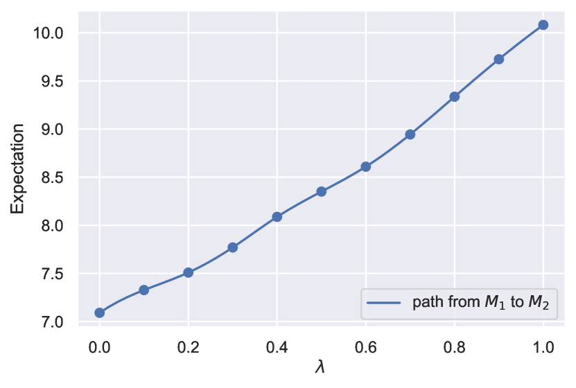
(a) Model switch TI

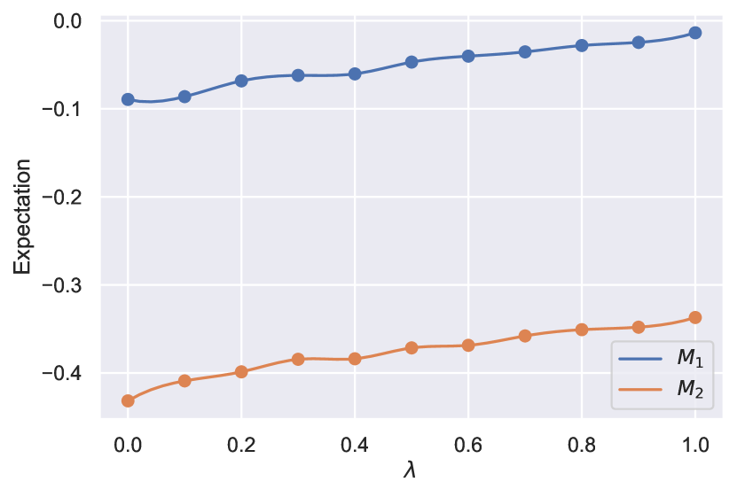
(b) Referenced TI

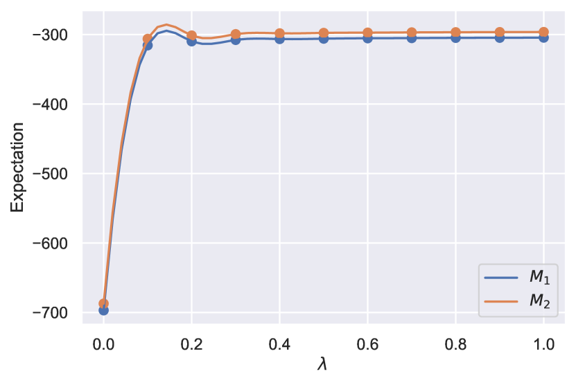
(c) PP₁₁

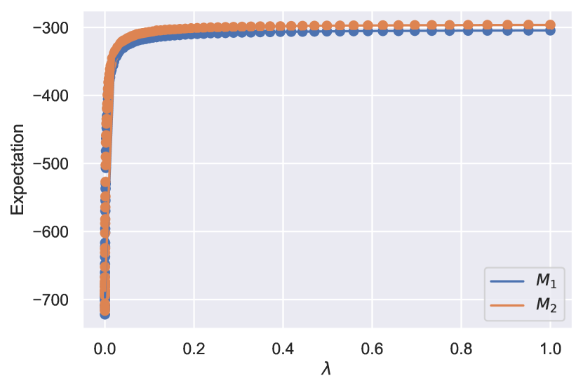
(d) PP₁₀₀

Figure 3: The HMC-evaluated expectation of $\mathbb{E}_{q(\lambda;\bm{\theta})}\left[\text{log\,}\frac{q(\bm{\theta})}{q_{\text{ref}}(\bm{\theta})}\right]$ vs coupling parameter $\lambda$ is given for models $M_{1}$ and $M_{2}$ for four methods of calculating the model evidence: model switch TI (a), referenced TI (b), power posteriors with 11 $\lambda$-placements (c) and power posteriors with 100 $\lambda$ placements (d). Model switch TI (a) creates the path directly between two competing densities, therefore only one line is shown (see Equation 2).

The 1-dimensional lines estimated by fitting a cubic spline to the expectation were integrated for each of the models to obtain the log-evidence for $M_{1}$ and $M_{2}$, and the log ratio of the two models’ evidences for the model switch TI. Rolling mean of the integral over 1500 iterations for referenced TI and PP₁₀₀ are shown in Figure 4 a-b. We can see from the plots, that referenced TI presents excellent convergence to the exact value, whereas PP₁₀₀ oscillates around it. In the same Figure 4, plots c-d show the distribution of log-evidence for each model generated by 15 runs of the three algorithms: Laplace approximation with sampled covariance matrix, referenced TI and PP₁₀₀. Although all three methods resulted in a log-evidence satisfactorily close to the exact solution, referenced TI was the most accurate and importantly, converged fastest.

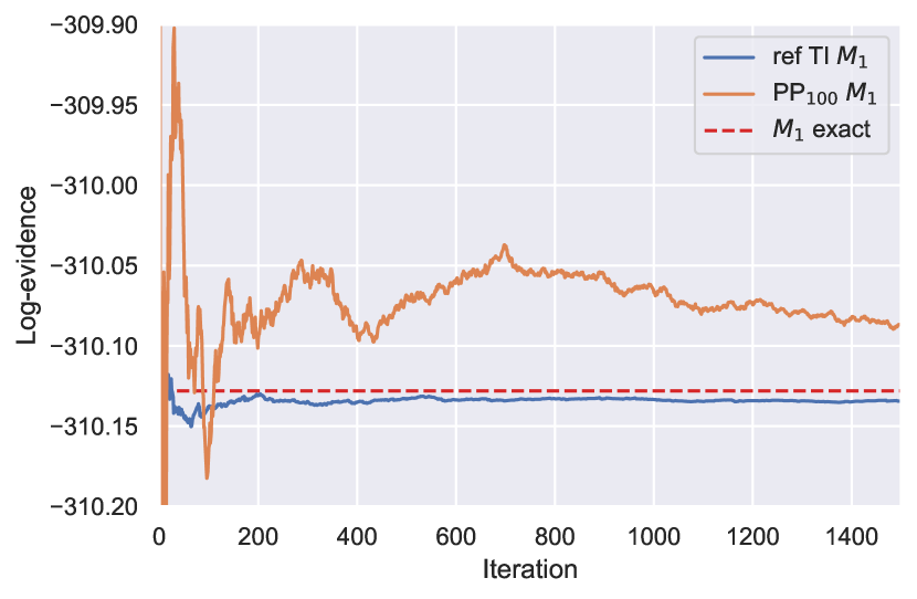
(a) $M_{1}$

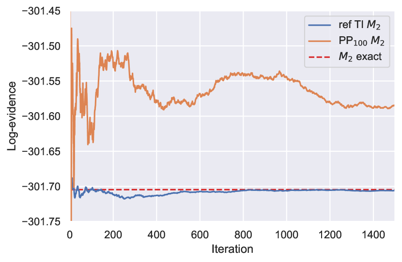
(b) $M_{2}$

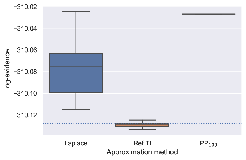
(c) $M_{1}$

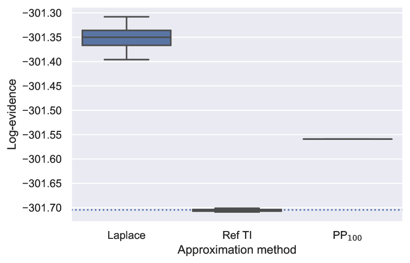
(d) $M_{2}$

Figure 4: Log-evidence of $M_{1}$ and $M_{2}$ for the three algorithms. (a) and (b) show the rolling mean of log-evidence of $M_{1}$ and $M_{2}$ over 1500 iterations per $\lambda$ obtained by referenced TI (blue line) and PP₁₀₀ (orange line) methods. The exact value is shown with red dashed line. (c) and (d) show the mean log-evidence of the two models evaluated over 15 runs of the three algorithms. The exact value of the log-evidence is shown with the dotted line.

The BFs calculated to assess whether model $M_{2}$ fits the data better than model $M_{1}$ and the number of iterations needed to achieve standard error of 0.5%, excluding the iterations needed for the MCMC burn-in, are presented in Table 2. Notably, both TI methods gave a BF very close to the exact value. Referenced TI performed the best out of tested methods—it converged faster than all other methods, requiring only 308 MCMC draws compared to 55,000 draws needed for the power posterior method or over 2,000 for the model switch TI. Referenced TI also showed excellent accuracy both in estimating individual model’s evidence and the BF.

Method	$BF_{21}$	MCMC steps
Exact	4552.35	-
Laplace approximation∗	6309.10	-
Model switch TI	4557.63	2,365
Referenced TI	4558.71	308
PP11	4463.71	41,514
PP100	4757.82	55,000

Table 2: Comparison of Bayes factors for radiata pine models for each method. Here we show $BF_{21}=\frac{M_{2}}{M_{1}}$ to determine whether model $M_{2}$ is better than model $M_{1}$. Both TI and referenced TI methods used 11 equidistant $\lambda$-s. Power posteriors method was used with 11 (PP₁₁) and 100 (PP₁₀₀) $\lambda$-s. Third column shows the total number of MCMC steps required to achieve standard error of 0.5%, excluding the burn-in steps. ^∗ - using sampled covariance matrix.

3.4 Model Selection for the COVID-19 Epidemic in South Korea

The final example of using referenced TI for calculating model evidence is fitting a renewal model to COVID-19 case data from South Korea. The data were obtained from https://opendata.ecdc.europa.eu/covid19/casedistribution/csv (accessed 19-07-2020) and contained time-series data of confirmed cases from 31-12-2019 to 18-07-2020. The model is based on the Bellman-Harris branching process whose expectation is the renewal equation. Its derivation and details are explained in Mishra et al. [48] and a short explanation of the model is provided in the Appendix. Briefly, the model is fitted to the time-series case data and estimates a number of parameters, including serial interval and the effective reproduction number, $R_{t}$. Number of cases for each day are modelled by a negative binomial distribution, with shape and overdispersion parameters estimated by a renewal equation. Three modification of the original model were tested:

• $GI=k$, $k=5,6,6.5,7,8,9,10,20$—fixing the mean of the $GI$ parameter, denoting the mean of Rayleigh-distributed generation interval (which we assume to be the same as the serial interval),

• $AR(k)$, $k=2,3,4$—autoregressive model with $k$ days lag,

• $W=k$, $k=1,2,3,4,7$—changing the length $k$ of the sliding window $W$.

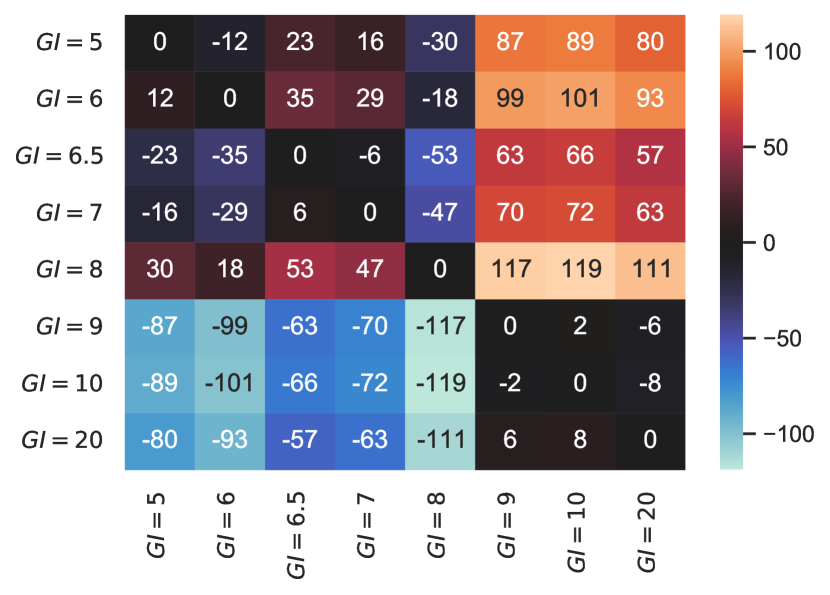
(a)

(b)

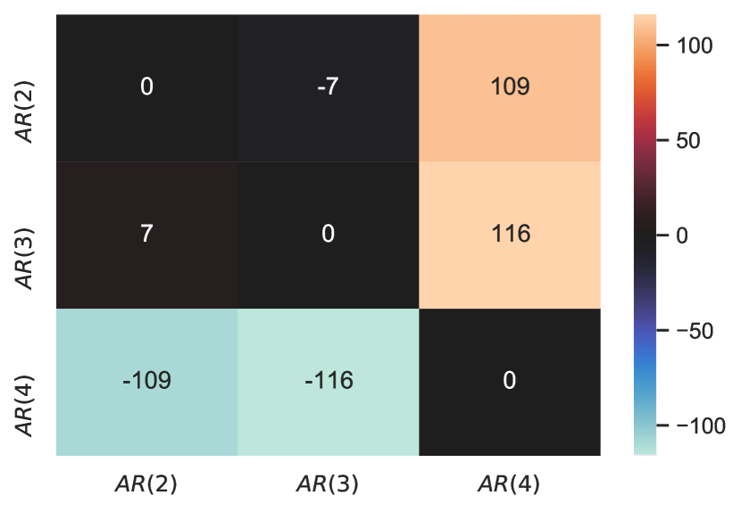
(c)

Figure 7: Logarithms of Bayes factors for the analysed COVID-19 renewal models, evaluated using the normalising constants ratios obtained by referenced TI. In each cell, the colour indicates the value of the $BF_{1,2}$ for models $M_{1}$ (row) and $M_{2}$ (column). Higher values, that is a brighter orange colour, suggest that $M_{1}$ is strongly better than $M_{2}$, and values below 0 in blue palette indicate that $M_{1}$ is worse than $M_{2}$. $GI=8$ performed best out of fixed $GI$ models, $W=2$ best out of sliding window models, and $AR(3)$ performed better than $AR(2)$ and $AR(4)$. For the interpretation of the BF values see [6].

Within each group of models, $GI$, $AR$ and $W$, we want to select the best model through the highest evidence method. For example, we want to check whether $GI=6$ fits the data better than $GI=10$, etc. The dimension of each model was dependent on the modifications applied, but in all the cases the normalising constant was a 40- to 200-dimensional integral. The log-evidence of each model was calculated using the Laplace approximation with a sampled covariance matrix, and then correction to the estimate was obtained using referenced TI method. Values of the log-evidence for each model calculated by both Laplace and referenced TI methods are given in Table 3. Interestingly, the favoured model in each group, that is the model with the highest log-evidence, was different when the evidence was evaluated using the Laplace approximation than when it was evaluated with referenced TI. For example, using the Laplace method, sliding window of length 7 was incorrectly identified as the best model, whereas with referenced TI window of length 2 was chosen to be the best among the tested sliding windows models, which agrees with the previous studies of the window-length selection in H1N1 influenza and SARS outbreaks [49]. This exposes how essential it is to accurately determine the evidence, even good approximations can result in misleading results. Log-Bayes factors for all model pairs within each of the three groups are shown in Figure 7 in the Appendix.

Model	Log-evidence (Laplace)	Correction	Log-evidence (ref TI)
GI=5	-1274	558	-716 [-715.6, -715.2]
GI=6	-1274	572	-703 [-703.3, -702.7]
GI=6.5	-1269	530	-739 [-738.6, -738.3]
GI=7	-1255	522	-732 [-732.4, -731.8]
GI=8	-1245	561	-685 [-685.5, -684.7]
GI=9	-1310	507	-803 [-802.8, -802.3]
GI=10	-1313	508	-805 [-805.1, -805.3]
GI=20	-1170	385	-796 [-796.3, -795.5]
AR(2)	-1207	496	-711 [-711.2, -710.6]
AR(3)	-1293	589	-704 [-704.7, -703.7]
AR(4)	-2166	1346	-821 [-820.6, -819.2.]
W=1	-1260	458	-802 [-802.1, -801.6]
W=2	-1069	278	-791 [-791.2, -790.7]
W=3	-1003	196	-807 [-807.5, -807.2]
W=4	-940	129	-811 [-811.1, -810.7]
W=7	-875	62	-814 [-813.7, -813.5]

Table 3: Log-evidence estimated by Laplace approximation, added referenced TI correction and total log-evidence from referenced TI, with 95% credible interval given in brackets. In each section, model with the highest log-evidence estimated by Laplace or referenced TI method is indicated in bold.

3.5 Interpretation of the COVID-19 model selection

The importance of performing model selection in a rigorous way is clear from Figure 5, where the posterior densities of parameters $\phi$ and $\sigma$ and the generated $R_{t}$ time-series are plotted for the models favoured by Laplace and referenced TI methods (meaning of the parameters is given in the Appendix). The differences in the densities and time-series show the pitfalls of selecting an incorrect model. For example, the parameter $\sigma$ was overestimated by the models selected by Laplace approximation in comparison to these selected by the referenced TI. The differences between the two favoured models were most extreme for the $GI=8$ and $GI=20$ models. While a $GI=8$ is plausible, even likely for COVID-19, $GI=20$ is implausible given observed data [50]. This is further supported by observing that for $GI=20$, favoured by the Laplace method, $R_{t}$ reached the value of over 125 in the first peak—around 100 more than for the $GI=8$. The second peak was also largely overestimated, where $R_{t}$ reached a value of 75.

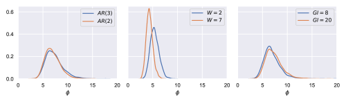
(a) Posterior distributions for overdispersion parameter $\phi$

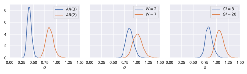
(b) Posterior distributions for $\sigma$ parameter

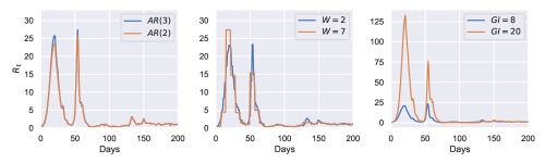
(c) $R_{t}$ generated by the favoured models

Figure 5: Posterior distributions for models’ parameters for models favoured by BFs using the Laplace approximation (orange lines) and referenced TI (blue lines).

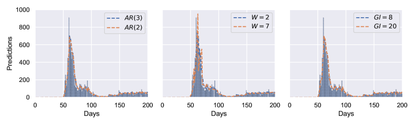
Figure 8: Cases of SARS-CoV-2 infections in South Korea from the data (shown with bars) and the cases predicted by different models. On each graph, predictions made by the model favoured by the Laplace approximation is shown with a blue dashed line, and predictions made by the referenced TI favoured models are shown with an orange dashed line. The lines in all three subplots are largely overlapping, revealing that all models fitted the case data similarly well.

We find it interesting to note that all models present a similar fit to the confirmed COVID-19 cases data, as shown by Figure 8 in the Appendix. This makes it impossible to select the best model through visual inspection and comparison of the model fits, or by using model selection methods that do not take the full posterior distributions into account. Although the models might fit the data well, other quantities generated, which are often of interest to the modeller, might be completely incorrect. Moreover, it emphasises the need to test multiple models before any conclusion or inference is undertaken, especially with the complex, hierarchical models. In epidemiology this is important as the modellers can be tempted to pick arbitrary parameters for their model, as long as the predictions fit the data. Although the fit might be accurate, other inferred parameters or uncertainty related to the predictions might be completely inappropriate for making any meaningful predictions.

In the radiata pine example, the contribution of TI to the marginalised likelihood estimated by the Laplace approximation was not substantial and using the Laplace approximation would suffice to make an informed model choice. However in this example, we see that the TI contribution is relatively large, and that it changes the decision to be made based on model evidence relative to the Laplace method. Moreover, from Table 3 we see that the evidence was the highest for the "boundary" models when Laplace approximation was applied. For example, for the sliding window length models, when the Gaussian approximation was applied, the log-evidence was monotonically increasing with the value of $W$ within the range of values that seem reasonable ($W=1-7$). In contrast, with referenced TI, the log-evidence is concave within the range of a priori reasonable parameters.

4 Discussion

The examples shown in Section 3 illustrate the applicability of the referenced TI algorithm for calculating model evidence. In the radiata pine example, referenced TI performed better than the other tested methods in terms of accuracy and speed. The power posteriors method required a much denser placement of the coupling parameters around $\lambda=0$, where the values are sampled purely from the prior distribution. In the case of referenced TI, at $\lambda=0$ values are sampled from the reference density, which should be closer to the original density (in the sense of Kullback–Leibler or Jensen-Shannon divergence), which results not only in a more accurate estimate of the normalising constant, but also much faster convergence of the MCMC samples. It also worth noting that referenced TI even performed better than the model switch TI method. A detailed theoretical characterisation of rates of convergence is beyond the scope of this article, nonetheless the empirical tests presented have consistently shown faster convergence than with comparative approaches. This is useful to know in the context of evaluating model evidence in complex hierarchical models where where each MCMC iteration is computationally demanding.

Although referenced thermodynamic integration and other methods using path-sampling have theoretical asymptotically exact Monte Carlo estimator limits, in practice a number of considerations affect accuracy. For example, biases will be introduced to the referenced TI estimate in practice if one endpoint density substantially differs from another. Then the volume of parameter space that must be explored to produce an unbiased estimate of the expectation cannot be sampled based on the reference density generating proposals within a practical number of iterations. The point is shown for a simple 1D example in Figure 6. Similarly, the larger the mismatch, the higher the variance and slower the expectation is to converge. This illustrates the advantage of using a reference that matches the posterior as closely as possible, as opposed to a typically wide reference like the prior distribution, that gives the characteristic divergence at $\lambda=0$ with power posteriors. Measures of density similarity in path sampling have been discussed by [24], however in practical terms there remains much scope for analysis of reference performance in terms of scaling with distribution dimension and type, which should be considered in detail in future work.

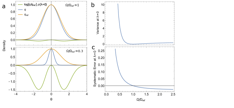
Figure 6: a) 1D examples to illustrate the bias and variance introduced with finite MCMC samples when $q$ and $q_{\text{ref}}$ are mismatched. In these examples $\Omega$ and $\Omega_{\text{ref}}$ denote the domain of the $99\%$ quartiles of $q$ and $q_{\text{ref}}$. b) A mismatch between $q$ and $q_{\text{ref}}$ ($\Omega$ and $\Omega_{\text{ref}}$) causes the variance of $\text{log}\frac{q}{q_{\text{ref}}}$ to increase, requiring more iterations to convergence. c) Similarly the mismatch causes the mass of the distribution for the expectation of $\text{log}\frac{q}{q_{\text{ref}}}$ (evaluated with respect to the reference distribution) to increase beyond the parameter range effectively sampled with finite iterations, in this example corresponding to the $99\%$ quartile of the sampling distribution, thus introducing a bias in the expectation.

Furthermore, the discretisation of the coupling parameter path in $\lambda$ can introduce a discretisation bias. For the power posteriors method, Friel et al. (2017) propose an iterative way of selecting the $\lambda$-placements to reduce the discretisation error [13]. Calderhead and Girolami (2009) test multiple $\lambda$-placements for 2 and 20 dimensional regression models, and report relative bias for each tested scenario [51]. In the referenced TI algorithm discretisation bias is however negligible — the use of the reference density results in TI expectations that are both small and have low variance, and therefore curvature with respect to $\lambda$. In our framework we use geometric paths with equidistant coupling parameters $\lambda$ between the un-normalised posterior densities, but there are other possible choices of the path constructions, for example a harmonic [12] or hypergeometric path [47]. This optimisation might be worthwhile exploring, however, as illustrated in Fig. 3b, the expectations evaluated vs $\lambda$ are typically near-linear with referenced TI suggesting limited gains, although the extent of this will differ from problem to problem.

In the application to the renewal model for the COVID-19 epidemic in South Korea, we showed that for a complex structured model, hypothesis selection by Laplace approximation of the normalising constant can give misleading results. Using referenced TI, we calculated model evidence for 16 models, which enabled a quick comparison between chosen pairs of competing models. Importantly, the evidence given by the referenced TI was not monotonic with the increase of one of the parameters, which was the case for the Laplace approximation in the models tested. The referenced TI presented here will similarly be useful in other situations particularly where the high-dimensional posterior distribution is uni-modal but non-Gaussian.

5 Conclusions

Normalising constants are fundamental in Bayesian statistics and allow the best model to be selected for given data. In this paper we give an account of referenced thermodynamic integration (TI), in terms of theoretical consideration regarding the choice of reference, and show how it can be applied to realistic practical problems. We show referenced TI allows efficient calculation of a single model’s evidence by sampling from geometric paths between the un-normalised density of the model and a judiciously chosen reference density — here, a sampled multivariate normal that can be generated and integrated with ease. The referenced TI approach was applied to several examples, in which normalising constants over 1 to 200 dimensional integrals were calculated. In the examples, the referenced TI approach had better convergence performance in terms of iterations to a cut-off convergence and minimum bias achievable compared to similar methods such as power posteriors or model switch thermodynamic integration. We showed the referenced TI method has practical utility for substantially challenging problems of model selection — in this instance concerning the epidemiology of infectious diseases — and suggest similar applicability in other fields of applied machine learning that rely on high-dimensional Bayesian models with non-inferential hyper-parameters.

Appendix A. COVID-19 Model

The COVID-19 model shown is based on the renewal equation derived from the Bellman-Harris process. The details of the model and its derivation are provided in Mishra et al. [48]. Here, we give a short overview of the $AR(2)$ model. The model has a Bayesian hierarchical structure and is fitted to the time-series data containing a number of new confirmed COVID-19 cases per day in South Korea, obtained from https://opendata.ecdc.europa.eu/covid19/casedistribution/csv. New infections $y(t)$ are modelled by a negative binomial distribution, with a mean parameter in a form of a renewal equation. The number of confirmed cases $y(t)$ is modelled as:

$$y\sim\text{NegBin}(f(t),\phi)\,,\\$$

where $\phi$ is an overdispersion or variance parameter and the mean of the negative binomial distribution is denoted as $f(t)$ and represents the daily case data through:

$$f(t)=R_{0}\int^{t}_{\tau=0}f(t-\tau)g(\tau)d\tau\,.$$

As the case data is not continuous but is reported per day, $f(t)$ can be represented in a discretised, binned form as:

$$f(t)=R_{t}\sum_{\tau<t}f(t-\tau)g(\tau)\,.$$

Here, $g(\tau)$ is a Raleigh-distributed serial interval with mean $GI$, which is discretised as

$$g_{s}=\int^{s+0.5}_{s-0.5}g(\tau)d\tau\text{ for }s=2,3,...\text{ and }g_{1}=\int^{1.5}_{0}g(\tau)d\tau\,.$$

$R_{t}$, the effective reproduction number, is parametrised as $R_{t}=\text{exp}(\epsilon_{t})$, with exponent ensuring positivity. $\epsilon_{t}$ is an autoregressive process with two-days lag, that is AR(2), with $\epsilon_{1}\sim N(-1,0.1)$, $\epsilon_{2}\sim N(-1,\sigma)$ and

$$\epsilon_{t}\sim N(\rho_{1}\epsilon_{t-1}+\rho_{2}\epsilon_{t-2},\sigma_{t})\text{ for }t=\{3,4,5,...\}.$$

The model’s priors are:

$$\sigma \sim N^{+}(0,0.2)\,,$$

$$\rho_{1} \sim N^{+}(0.8,0.05)\,,$$

$$\rho_{2} \sim N^{+}(0.1,0.05)\,,$$

$$\phi \sim N^{+}(0,5)\,,$$

$$GI \sim N^{+}(0.01,001)\,.$$

Modification were applied to this basic model, to obtain the different variants of the model as described in Section 3. First group of models analysed was the AR(2) model described above, but with the $GI$ parameter fixed to a certain value instead of inferring that parameter from the data. $AR(3)$ and $AR(4)$ models had additional parameters $\rho_{3}$ and $\rho_{4}$, which allow to model the autoregressive process with a longer lag (3- and 4- days respectively). Finally, models $W=k$, $k=1,..,7$ were similar to the $AR(2)$ model, but the underlying assumption of these models is that the $R_{t}$ stays constant for the duration of the length of the sliding window $W=k$.

References

- [1] Mrinank Sharma, Sören Mindermann, Jan Brauner, Gavin Leech, Anna Stephenson, Tomáš Gavenčiak, Jan Kulveit, Yee Whye Teh, Leonid Chindelevitch and Yarin Gal “How Robust are the Estimated Effects of Nonpharmaceutical Interventions against COVID-19?” In Advances in Neural Information Processing Systems 33, 2020
- [2] Seth Flaxman, Swapnil Mishra, Axel Gandy, H Juliette T Unwin, Thomas A Mellan, Helen Coupland, Charles Whittaker, Harrison Zhu, Tresnia Berah and Jeffrey W Eaton “Estimating the effects of non-pharmaceutical interventions on COVID-19 in Europe” In Nature 584.7820 Nature Publishing Group, 2020, pp. 257–261
- [3] Nicholas C. Grassly and Christophe Fraser “Mathematical models of infectious disease transmission” In Nature Reviews Microbiology 6, 2008, pp. 477–487 DOI: 10.1038/nrmicro1845
- [4] Libo Sun, Chihoon Lee and Jennifer A. Hoeting “Parameter inference and model selection in deterministic and stochastic dynamical models via approximate Bayesian computation: modeling a wildlife epidemic” In Environmetrics 26.7, 2015, pp. 451–462 DOI: 10.1002/env.2353
- [5] Theresa Stocks, Tom Britton and Michael Höhle “Model selection and parameter estimation for dynamic epidemic models via iterated filtering: application to rotavirus in Germany” In Biostatistics 21.3, 2018, pp. 400–416 DOI: 10.1093/biostatistics/kxy057
- [6] Robert E. Kass and Adrian E. Raftery “Bayes Factors” In Journal of the American Statistical Association 90.430, 1995, pp. 773–795 eprint: https://www.stat.cmu.edu/~kass/papers/bayesfactors.pdf
- [7] Charles H Bennett “Efficient estimation of free energy differences from Monte Carlo data” In Journal of Computational Physics 22.2 Elsevier, 1976, pp. 245–268
- [8] Xiao-Li Meng and Wing Hung Wong “Simulating ratios of normalizing constants via a simple identity: a theoretical exploration” In Statistica Sinica JSTOR, 1996, pp. 831–860
- [9] John Skilling “Nested Sampling for General Bayesian Computation” In Bayesian Analysis 1.4, 2006, pp. 833–860 URL: https://projecteuclid.org/download/pdf_1/euclid.ba/1340370944
- [10] Michael Habeck “Evaluation of marginal likelihoods via the density of states” In Artificial Intelligence and Statistics, 2012, pp. 486–494
- [11] John G. Kirkwood “Statistical Mechanics of Fluid Mixtures” In The Journal of Chemical Physics 3.5, 1935, pp. 300–313 DOI: 10.1063/1.1749657
- [12] Andrew Gelman and Xiao-Li Meng “Simulating normalizing constants: From importance sampling to bridge sampling to path sampling” In Statistical science JSTOR, 1998, pp. 163–185
- [13] Nial Friel, Merrilee Hurn and Jason Wyse “Improving power posterior estimation of statistical evidence” In Statistics and Computing, 2017, pp. 1165–1180 DOI: https://doi.org/10.1007/s11222-016-9678-6
- [14] Nicolas Lartillot and Hervé Philippe “Computing Bayes Factors Using Thermodynamic Integration” In Systematic Biology 55.2, 2006, pp. 195–207 DOI: 10.1080/10635150500433722
- [15] Wangang Xie, Paul O. Lewis, Yu Fan, Lynn Kuo and Ming-Hui Chen “Improving Marginal Likelihood Estimation for Bayesian Phylogenetic Model Selection” In Systematic Biology 60.2, 2010, pp. 150–160 DOI: 10.1093/sysbio/syq085
- [16] Evan J. Williams “Regression Analysis” Wiley, 1959
- [17] Paul Adrien Maurice Dirac “The quantum theory of the emission and absorption of radiation” In Proceedings of the Royal Society of London. Series A, Containing Papers of a Mathematical and Physical Character 114.767 The Royal Society London, 1927, pp. 243–265
- [18] Murray Gell-Mann and Keith A Brueckner “Correlation energy of an electron gas at high density” In Physical Review 106.2 APS, 1957, pp. 364
- [19] Lidunka Vocadlo and Dario Alfe “Ab initio melting curve of the fcc phase of aluminum” In Phys Rev B 65.21 AMERICAN PHYSICAL SOC, 2002
- [20] Andrew Ian Duff, Theresa Davey, Dominique Korbmacher, Albert Glensk, Blazej Grabowski, Jörg Neugebauer and Michael W Finnis “Improved method of calculating ab initio high-temperature thermodynamic properties with application to ZrC” In Physical Review B 91.21 APS, 2015, pp. 214311
- [21] Nial Friel and Anthony N. Pettitt “Marginal likelihood estimation via power posteriors” In Journal of the Royal Statistical Society: Series B (Statistical Methodology) 70.3, 2008, pp. 589–607 DOI: 10.1111/j.1467-9868.2007.00650.x
- [22] Nial Friel and Jason Wyse “Estimating the evidence: a review” In Statistica Neerlandica 66.3, 2012, pp. 288–308 DOI: 10.1111/j.1467-9574.2011.00515.x
- [23] Ewan Cameron and Anthony Pettitt “Recursive pathways to marginal likelihood estimation with prior-sensitivity analysis” In Statistical Science 29.3 Institute of Mathematical Statistics, 2014, pp. 397–419
- [24] Geneviève Lefebvre, Russell Steele and Alain C Vandal “A path sampling identity for computing the Kullback–Leibler and J divergences” In Computational statistics & data analysis 54.7 Elsevier, 2010, pp. 1719–1731
- [25] Yu Fan, Rui Wu, Ming-Hui Chen, Lynn Kuo and Paul O Lewis “Choosing among partition models in Bayesian phylogenetics” In Molecular Biology and Evolution 28(1), 2011, pp. 523–532 DOI: 10.1093/molbev/msq224
- [26] Guy Baele, Philippe Lemey and Marc A Suchard “Genealogical Working Distributions for Bayesian Model Testing with Phylogenetic Uncertainty” In Systematic Biology 65(2), 2016, pp. 250–264 DOI: 10.1093/sysbio/syv083
- [27] Nikolai N. Bogolubov Jr “On model dynamical systems in statistical mechanics” In Physica 32.5 Elsevier, 1966, pp. 933–944
- [28] Alexander L. Kuzemsky “Variational principle of Bogoliubov and generalized mean fields in many-particle interacting systems” In International Journal of Modern Physics B 29.18 World Scientific, 2015, pp. 1530010
- [29] Jun Zhang “The application of the Gibbs-Bogoliubov-Feynman inequality in mean field calculations for Markov random fields” In IEEE Transactions on Image Processing 5.7 IEEE, 1996, pp. 1208–1214
- [30] Radford M. Neal and Geoffrey E. Hinton “A view of the EM algorithm that justifies incremental, sparse, and other variants” In Learning in graphical models Springer, 1998, pp. 355–368
- [31] Michael I. Jordan, Zoubin Ghahramani, Tommi S. Jaakkola and Lawrence K. Saul “An introduction to variational methods for graphical models” In Machine learning 37.2 Springer, 1999, pp. 183–233
- [32] James Ridgway “Computation of Gaussian orthant probabilities in high dimension” In Statistics and computing 26.4 Springer, 2016, pp. 899–916
- [33] Dario Azzimonti and David Ginsbourger “Estimating orthant probabilities of high-dimensional Gaussian vectors with an application to set estimation” In Journal of Computational and Graphical Statistics 27.2 Taylor & Francis, 2018, pp. 255–267
- [34] Donald B. Owen “Orthant probabilities” In Wiley StatsRef: Statistics Reference Online Wiley Online Library, 2014
- [35] Tetsuhisa Miwa, AJ Hayter and Satoshi Kuriki “The evaluation of general non-centred orthant probabilities” In Journal of the Royal Statistical Society: Series B (Statistical Methodology) 65.1 Wiley Online Library, 2003, pp. 223–234
- [36] Robert N. Curnow and Charles W. Dunnett “The numerical evaluation of certain multivariate normal integrals” In The Annals of Mathematical Statistics JSTOR, 1962, pp. 571–579
- [37] Harold Ruben “An Asymptotic Expansion for the Multivariate” In Journal of Research of the National Bureau of Standards: Mathematics and mathematical physics. B 68 The Bureau, 1964, pp. 3
- [38] M. Brown “A generalized error function in n dimensions” In U.S. Naval Missile Center, Theorethical Analysis Division, 1963 URL: https://apps.dtic.mil/dtic/tr/fulltext/u2/401722.pdf
- [39] Matthew D Hoffman and Andrew Gelman “The No-U-Turn sampler: adaptively setting path lengths in Hamiltonian Monte Carlo” In J. Mach. Learn. Res. 15.1, 2014, pp. 1593–1623
- [40] Bob Carpenter, Andrew Gelman, Matthew Hoffman, Daniel Lee, Ben Goodrich, Michael Betancourt, Marcus Brubaker, Jiqiang Guo, Peter Li and Allen Riddell “Stan: A Probabilistic Programming Language” In Journal of Statistical Software, Articles 76.1, 2017, pp. 1–32 DOI: 10.18637/jss.v076.i01
- [41] Stan Development Team “Stan for epidemiology” URL: https://epidemiology-stan.github.io/
- [42] John N. Bahcall and R. A. Wolf “Star distribution around a massive black hole in a globular cluster” In The Astrophysical Journal 209, 1976, pp. 214–232
- [43] Tosio Kato “On the eigenfunctions of many-particle systems in quantum mechanics” In Communications on Pure and Applied Mathematics 10.2 Wiley Online Library, 1957, pp. 151–177
- [44] Robert Piessens, Elise Kapenga, Christian Ueberhuber and David Kahaner “QUADPACK: A Subroutine Package for Automatic Integration” Springer, 1983
- [45] SciPy.org “SciPy: Open Source Scientific Tools for Python: scipy.integrate” URL: https://docs.scipy.org/doc/scipy/reference/integrate.html
- [46] Pauli Virtanen, Ralf Gommers, Travis E. Oliphant, Matt Haberland, Tyler Reddy, David Cournapeau, Evgeni Burovski, Pearu Peterson, Warren Weckesser, Jonathan Bright, Stéfan J. van der Walt, Matthew Brett, Joshua Wilson, K. Jarrod Millman, Nikolay Mayorov, Andrew R. J. Nelson, Eric Jones, Robert Kern, Eric Larson, CJ Carey, İlhan Polat, Yu Feng, Eric W. Moore, Jake Vand erPlas, Denis Laxalde, Josef Perktold, Robert Cimrman, Ian Henriksen, E. A. Quintero, Charles R Harris, Anne M. Archibald, Antônio H. Ribeiro, Fabian Pedregosa, Paul van Mulbregt and SciPy 1. 0 Contributors “SciPy 1.0: Fundamental Algorithms for Scientific Computing in Python” In Nature Methods 17, 2020, pp. 261–272 DOI: https://doi.org/10.1038/s41592-019-0686-2
- [47] Silia Vitoratou and Ioannis Ntzoufras “Thermodynamic Bayesian model comparison” In Statistics and Computing, 2017, pp. 1165–1180 DOI: https://doi.org/10.1007/s11222-016-9678-6
- [48] Swapnil Mishra, Tresnia Berah, Thomas A. Mellan, H. Juliette T. Unwin, Michaela A. Vollmer, Kris V. Parag, Axel Gandy, Seth Flaxman and Samir Bhatt “On the derivation of the renewal equation from an age-dependent branching process: an epidemic modelling perspective” In arXiv preprint arXiv:2006.16487, 2020
- [49] Kris V. Parag and Christl A. Donnelly “Using information theory to optimise epidemic models for real-time prediction and estimation” In PLOS Computational Biology 16.7 Public Library of Science, 2020, pp. 1–20 DOI: 10.1371/journal.pcbi.1007990
- [50] Qifang Bi, Yongsheng Wu, Shujiang Mei, Chenfei Ye, Xuan Zou, Zhen Zhang, Xiaojian Liu, Lan Wei, Shaun A Truelove, Tong Zhang, Wei Gao, Cong Cheng, Xiujuan Tang, Xiaoliang Wu, Yu Wu, Binbin Sun, Suli Huang, Yu Sun, Juncen Zhang, Ting Ma, Justin Lessler and Tiejian Feng “Epidemiology and transmission of COVID-19 in 391 cases and 1286 of their close contacts in Shenzhen, China: a retrospective cohort study” In The Lancet Infectious Disease 20, 2020, pp. 911–919 DOI: doi: 10.1016/S1473-3099(20)30287-5
- [51] Ben Calderhead and Mark Girolami “Estimating Bayes factors via thermodynamic integration and population MCMC” In Computational Statistics & Data Analysis 53.12, 2009, pp. 4028 –4045 DOI: https://doi.org/10.1016/j.csda.2009.07.025