The impact of COVID-19 on relative changes in aggregated mobility using mobile-phone data

Abstract

Evaluating relative changes leads to additional insights that would remain hidden when only evaluating absolute changes. We analyze a dataset describing the mobility of mobile phones in Austria before, during COVID-19 lock-down measures until recently.

By applying compositional data analysis we show that formerly hidden information becomes available: we see that the elderly population groups increase relative mobility and that the younger groups, especially on weekends, also do not decrease their mobility as much as the others.

1 Introduction

The usage data of mobile-phones is used in a variety of different areas, such as during the COVID-19 pandemic [1, 2, 3, 4, 5, 6, 7, 8, 9, 10, 11], customer segmentation [12], identification of personality traits and lifestyle [13, 14], the analysis of large social networks [15, 16, 17], hotspot detection [18], prediction of movement [19], mode of transport identification [20], credit scoring [21], disaster recovery [22, 23], analysis of sleeping behavior of the population [24], migration [25] and land usage classification [26, 27].

The location of a mobile-phone is known for the Mobile Network Operator (MNO) of the Global System for Mobile Communication (GSM) network. We have partnered with an MNO in Austria to get access to such anonymized data. We have defined an aggregation method to understand the overall aggregated mobility of the whole population. Our data set as well as the aggregation, anonymization approach and the various phases of the lock-down are outlined in detail in [28].

With the outbreak of COVID-19 and the subsequent lock-down in Austria, the mobility behavior of the population has changed significantly. This is reflected in the mobility data derived from mobile-phone information [28]. To measure mobility, an appropriate measure needs to be established which reflects the mobility. One possibility is the radius of gyration (ROG) [29]. It is formally defined below, and refers to the time-weighted distance of the movement locations to the main location. We compute it on a daily level. Its unit is meters, and the values are strictly positive. In this work the analyze the aggregated (median) ROG of the whole population of Austria for various groups as a time series. The groups are defined by gender- or age groups.

Traditionally, a comparison is made in terms of absolute information, i.e., the ROG time series values of the different groups are analyzed in their unit of meters. We have conducted such an analysis [30] which focuses on gender differences.

An alternative is to compare relative information, for example the ROG of the males with respect to females, or in terms of the ratio males to females. This leads to a dimensionless time series, and to a different aspect of data analysis which emphasizes the differences between the individual groups. A joint increase or decrease in both groups may not lead to a big change of the ratio. On the other hand, the ratio will change if the values of one group increase, and at the same time they decrease in the other group, or vice versa. Here again, the relative change rather than the absolute change is important. For example, if the ROG changes from 1000m to 2000m in one group, and from 2000m to 1000m in the other group, the ratio would change from 1/2 to 2. The same change could be observed if the absolute values in both groups would be bigger by a factor of 10. Thus, absolute values are no longer relevant in this consideration, because a multiplication by any positive constant leads to the same ratio. This is still trivial in case of comparing two groups, but it is no longer straightforward when relative information of several groups, such as age classes, should be compared. Compositional data analysis is devoted to this problem of analyzing relative information [31, 32, 33]. In fact, compositional data analysis is frequently used in geosciences, but also more and more in other fields such as biology [34], bioinformatics [35], economics [36], marketing [37], medicine [38], etc.

We contribute compositional analysis of the movement data during the COVID-19 analysis which comes to the conclusion that special groups (elderly and young cohorts during weekends) need an additional caring treatment to improve their security.

This work is structured as follows. In Section 2.1 we give a brief mathematical introduction to compositional data analysis. Section 2.2 provides more details about the mobile-phone data used and about the quantities derived. In addition to the mobility measured as the ROG we will furthermore investigate the call duration per day, again aggregated by the median. Section 3 presents comparisons of the analysis based on absolute and on relative information, and the final Section 4 summarizes the findings.

2 Materials and methods

2.1 Compositional data analysis

From the point of view of compositional data analysis, a composition is defined as multivariate information, consisting of strictly positive values, where the absolute numbers as such are not of interest, and only relative information is relevant for the analysis [33]. A composition can be given for example by the median ROG values of different age categories for a certain day, and every age category is denoted as a compositional part. We use the notation $x_{1},\ldots,x_{D}$ for the compositional parts of $D$ categories, and the composition is written as the (column) vector $\mathbf{x}=(x_{1},\ldots,x_{D})^{\prime}$. For every day recorded in our data base we will observe such a composition, which in fact leads to a multivariate compositional time series. The interest is in relative information in terms of the ratios, and thus all pairs $x_{j}/x_{k}$, for $j,k=1,\ldots,D$, should be considered in the analysis. Obviously, the pairs for $j=k$ are not relevant, and pairs of the reverse ratio $x_{k}/x_{j}$ do not contain potentially new information. This motivates to consider the logarithm of the ratios, $\ln(x_{j}/x_{k})$, so-called log-ratios. The reverse ratios have a different sign, and thus do not need to be considered, and their variance is the same as for the original ratio. Moreover, the distributions of log-ratios tend to be more symmetric than without a logarithm [32].

Still, the resulting $D(D-1)$ pairs $\ln(x_{j}/x_{k})$, for $k>j$, only live in a subspace of dimension $\leq D-1$ [33], and thus it is natural to aggregate this information. Consider an aggregation

$$y_{1}=\frac{1}{D}\left(\ln\frac{x_{1}}{x_{2}}+\ldots+\ln\frac{x_{1}}{x_{D}}\right)=\ln\frac{x_{1}}{g(\mathbf{x})}\ ,$$ (1)

where

$$g(\mathbf{x})=\sqrt[D]{\prod_{j=1}^{D}x_{j}}$$

is the geometric mean of the composition $\mathbf{x}$. Then, $y_{1}$ represents all relative information about the part $x_{1}$ to the other parts in the composition in a form of an average of the log-ratios. This leads to the definition of so-called centered log-ratio (CLR) coefficients [31]

$$\mathbf{y}=(y_{1},\ldots,y_{D})^{\prime}\quad\mbox{ with }\quad y_{j}=\ln\frac{x_{j}}{g(\mathbf{x})}\ .$$ (2)

The vector $\mathbf{y}$ contains all relative information about $\mathbf{x}$ in the above sense. It consists of $D$ components $y_{j}$ which are associated with the relative information about the corresponding part $x_{j}$. However, it turns out that $y_{1}+\ldots+y_{D}=0$, and thus a representation of data in terms of CLR coefficients leads to singularity [33]. Although there are ways to circumvent this issue [33], we will proceed with CLR coefficients for the following analysis for simplicity.

Consider now a multivariate compositional time series $\mathbf{x}_{t}=(x_{t1},\ldots,x_{tD})^{\prime}$, for the time points $t=1,\ldots,T$, and the observations $x_{tj}$ for each part $j\in\{1,\ldots,D\}$. The time series expressed in CLR coefficients is $\mathbf{y}_{t}=(y_{t1},\ldots,y_{tD})^{\prime}$, with $y_{tj}=\ln(x_{tj}/g(\mathbf{x}_{t}))$, with the geometric mean $g(\mathbf{x}_{t})=(\prod_{j=1}^{D}x_{tj})^{1/D}$ per time point. Since this data representation only reflects relative information of the time series, an additional visualization of the absolute time series values can be interesting to get a more complete picture.

The CLR coefficients result in multivariate data that can be analyzed with the traditional multivariate statistical methods [33]. A prominent way to represent the information in a lower-dimensional space is to use principal component analysis (PCA). Since PCA is sensitive to data outliers or inhomogeneous data, robust versions have been proposed, also in the compositional data analysis framework [33]. The resulting loadings and scores are commonly represented in a biplot to get an overview of the multivariate data [39].

2.2 Mobile-phone data

In this work we analyze two measures obtained from the mobile phone data, the call duration and the radius of gyration ROG. While the meaning of the former is straightforward, the latter needs to be defined.

Consider an individual $i:=i(t)$ at a certain day $t\in\{1,\ldots,T\}$. For reasons of data privacy, the index of the individual will change every day. The data is made available to the researchers already anonymized with a daily changing key.

Furthermore, the current location of the individual’s mobile phone is available at the time points $t_{\tau}=t+\tau_{t}$, for a number of time points $T_{t}$ per day, where $\tau_{t}\in[0,1)$. The corresponding $x$- and $y$-coordinates are denoted by $(\xi_{it_{\tau}},\eta_{it_{\tau}})$. With this information, the stay duration $l_{it_{\tau}}$ for individual $i$ at time point $t_{\tau}$ can be computed, which is used to calculate a weighted average $(\bar{\xi}_{it},\bar{\eta}_{it})=\left(\frac{\sum_{t_{\tau}}l_{it_{\tau}}\xi_{it_{\tau}}}{\sum_{t_{\tau}}l_{it_{\tau}}},\frac{\sum_{t_{\tau}}l_{it_{\tau}}\eta_{it_{\tau}}}{\sum_{t_{\tau}}l_{it_{\tau}}}\right)$ for individual $i$ for day $t$. These coordinates are in the middle of the area covered by all the locations which were visited during the day and are dominated by the two most prominently used (longest used) locations: home and work location.

Denote $d^{2}_{it_{\tau}}=(\bar{\xi}_{it}-\xi_{it_{\tau}})^{2}+(\bar{\eta}_{it}-\eta_{it_{\tau}})^{2}$ as the squared Euclidean distance between the coordinates $(\bar{\xi}_{it},\bar{\eta}_{it})$ and $(\xi_{it_{\tau}},\eta_{it_{\tau}})$. This requires the coordinate system to be local in order to obtain valid, i.e. less distorted results. Otherwise, a Haversine distance could be used instead in case of epsg:4326 WGS-84 projection of the coordinates.

The ROG for individual $i$ and day $t$ is then defined as

$$R_{it}=\sqrt{\frac{\sum_{t_{\tau}}d^{2}_{it_{\tau}}}{\sum_{t_{\tau}}l_{it_{\tau}}}},$$ (3)

and it thus represents a distance to the center of all the places of stay during that day $t$ weighted by the lengths of the stay duration at the different places.

Details are available and especially a description of how the large quantity of data was handled is available in [28].

Using additional metadata, an individual $i$ can be assigned to a gender group (female, male), to an age group (here we consider the age groups in 15 year intervals: 15-29, 30-44, 45-59, 60-74, and 75$+$), and to an Austrian district of the daily night location to derive the groups. Since the distributions are generally very right-skewed, we work with the median per group and day in the following and also ensure k-anonymity for each one.

The resulting time series can be directly investigated in terms of their absolute information, and they can be compared to an analysis based on relative information.

3 Results

3.1 Mobility measured by ROG

The results reported in this section refer to the median values of the ROG per group. To begin with, Figure 1 shows the absolute values for the females (top) and males (bottom) for different age groups. The legend indicates the considered age groups: 15 for age 15-29, 30 for age 30-44, 45 for age 45-59, 60 for age 60-74, and 75 for age elder than 75. For all of the following time series plots, the vertical dashed lines indicate the date March 16^th, 2020, when the restrictions came into action, and the date April 6^th, 2020, when they were relaxed. The data considered here are from the period February 1^st until August 9^th, 2020. The lock-down is clearly visible in the plots by an abrupt decay of the median ROG values in all age classes for both genders. After the lock-down, the order of the values still remains the same, from the eldest group with the smallest values, and the youngest group with the highest values, but it is on a much smaller level. The level then increased more or less systematically until the middle of June. Afterwards, the level is not changing a lot, it is lower than at the beginning, and weekly patterns are clearly visible. Note that these weekly time series patterns that are very regular at the beginning are getting somehow distorted, partially also due to holidays (April 13^th, May 1^st, May 21^th, June 1^st, June 11^th), and they never get back to this regularity.

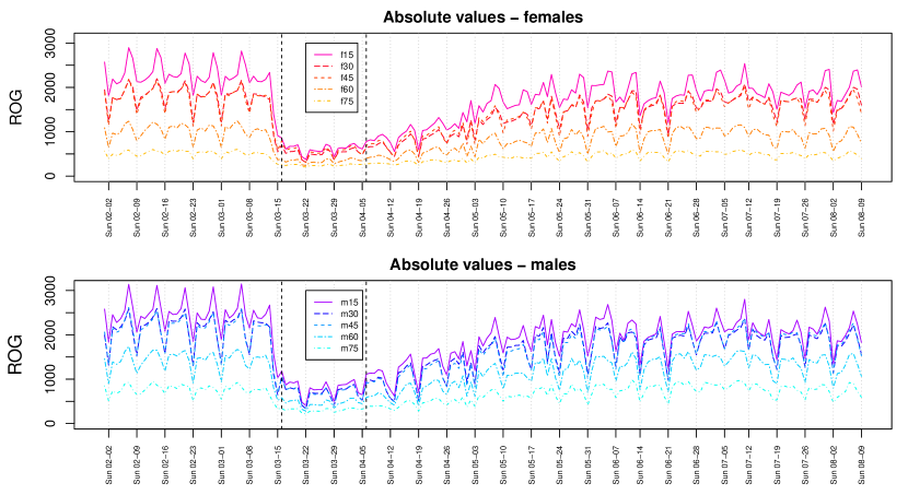
Figure 1: Median ROG values for different age groups over time for females (top) and males (bottom) in different age groups.

Figure 2 focuses on the relative information contained in the median ROG values. We consider the female age groups and the male age groups separately as two compositions. The plots show the corresponding CLR coefficients for females (top) and males (bottom). While in Figure 1 we have essentially seen a decline of all values at the beginning of the lock-down phase, followed by an increase, we did not pay attention how differently the age groups declined and increased. This is the purpose of the relative view in Figure  2, where we mainly investigate the developments of the age groups to each other.

In both plots of Figure  2 we can see roughly the same pattern after the lock-down: the biggest relative changes are visible for the youngest and the oldest age group, but they go into different directions. While group 15 had the biggest decline, group 75$+$ increased the values relative to the other age groups. This seems to be counter-intuitive, but it can be explained by the fact that the geometric mean also went down significantly, and the ratio of the values of group 75$+$ to the geometric mean then even increased after the lock-down. Another interesting phenomenon is that the groups 60 and 75$+$ show the biggest increase in mobility (in a relative sense) during the weekends in this lock-down period. Although on a different level, the values from July show a similar structure to those from February. It is interesting to note that the youngest age group 15 shows a somehow mirrored weekly pattern compared to the elder age groups. This is not visible when looking at the absolute values in Figure 1.

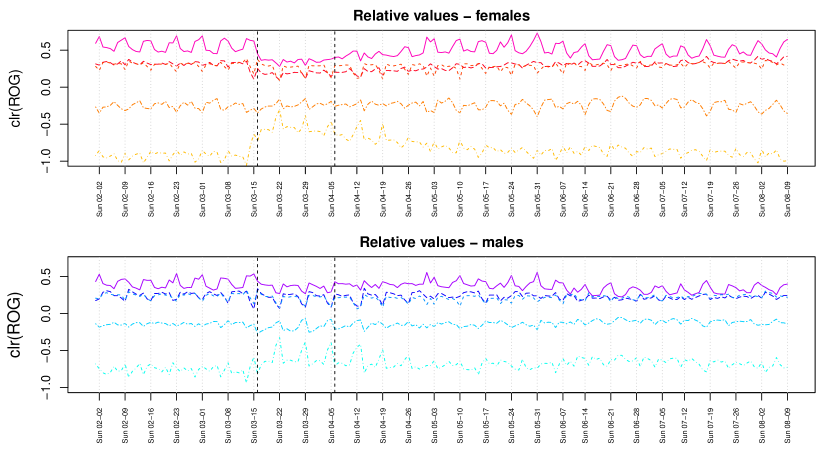
Figure 2: CLR coefficients of median ROG values for the female (top) and the male (bottom) composition. For the legend see Figure 1.

Relative information could also be understood in terms of data proportions. In particular, one could compute the proportion of a group on the total per time point, which in fact corresponds to normalizing the data per time point to a value of 1. Such a proportional presentation is shown in Figure 3 for the ROG values of the female age groups. Obviously, the information contained in this representation is different from CLR coefficients which focus on log-ratio information. One can hardly see any differences between the lock-down period and the remaining period, and thus this kind of “relative view” is not valuable for the analysis.

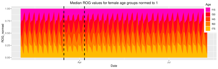
Figure 3: Proportional presentation of the median ROG values for the female age groups. For each time point, the data are normalized to a value of 1.

The median ROG values for the female and male age groups are analyzed in the following with PCA. Here, the method ROBPCA [40] is taken, a robust version of PCA which downweights outlying observations. Figure 4 shows the biplot of the first two principal components (PCs) for the clr coefficients. The coloring is according to the time phases: green before the lock-down, pink during the lock-down period, purple after lock-down until mid of June, and light-blue after this period. The left biplot for the females identifies these four periods as clear clusters, while there is more overlap visible in the right biplot for the males. For the females, the direction of the first PC (71% explained variance) shows a transition of the relative ROG values from the young generation (f15, f30) before lock-down to the old (f75) one during lock-down, and then back to the center. Thus, younger and elder females show a contrasting behavior in this time period, which was already observed in Figure  2 (top panel). The second PC (21% explained variance) shows also differences between the time periods, but it also reveals weekend effects. Especially on Sundays, the mobility for group f15 was bigger before and after lock-down, but it moved to group f75 during the lock-down phase.

The data structure in the biplot for the males (right plot) looks a bit different, but leads to similar conclusions. PC1 explains 69% and PC2 25% of the variance. Groups m75 and m15 have a similarly diverging behavior of Sunday mobility as observed for the females. The weekdays of the lock-down phase are in the center of the distribution, while for the females they were clearly moved towards group f75. On the other hand, the weekdays in the first time period (February 1^st - March 15^th) are better distinguishable from the weekdays of the last period (June 15 - August 9); a possible explanation is the fact that the working male population changed the mobility behavior more significantly than that of females due to home office.

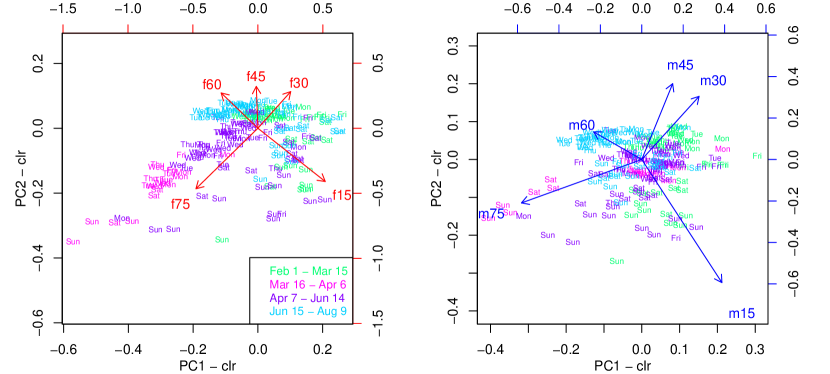
Figure 4: Biplots of the CLR coefficients of the median ROG values for females (left) and male (right) age groups. Green color for period before the lock-down, pink for lock-down period, purple after lock-down until mid of June, and light-blue after this period.

A quite contrasting view is revealed in Figure 5, which shows the robust PCA results for the absolute values of ROG, for females (left) and males (right). In both analyses, PC1 explains 98% of the variability, and this direction essentially reflects the big change of the ROG over this time period. Otherwise, there is not much information left in these analyses, which reflects the limited usefulness of absolute information if the task is to compare age groups.

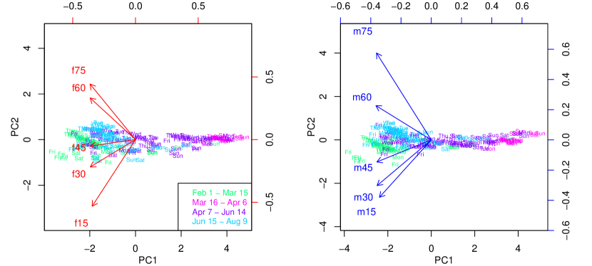
Figure 5: Biplots of the (absolute) median ROG values for females (left) and male (right) age groups. Green color for period before the lock-down, pink for lock-down period, purple after lock-down until mid of June, and light-blue after this period.

3.2 Interaction measured by call duration

Figure 6 investigates the median call duration, reported in seconds, again for the two genders and the age groups. The absolute values are shown in the upper plot jointly for males and females. Here we observe the reverse ordering of the age groups compared to the plots for the ROG values: the lowest values are for the youngest group, and the biggest for the oldest group. The values of the females are systematically higher than those of the males. It is interesting to see that the call durations already started to increase one week before the lock-down. While the ROG time series had their peaks during the weekend, we have the opposite here. This pattern, however, seems to change after the lock-down for group f75 (uppermost line), and it went back to normality only later on.

The bottom plot of Figure 6 presents the CLR coefficients, which are separately calculated for females and males, but presented here jointly for easy comparison. Although the absolute values of the youngest age group also increased with the lock-down, the increase was smaller compared to the other groups, which is reflected by decreasing CLR coefficients. The pattern of f15 and m15 has also an interesting structure: Before the lock-down, the groups had quite different behavior within their gender-group, but during the lock-down phase they became quite similar. From June on, they show again a similar behavior as at the beginning. Another interesting phenomenon can be seen after the lock-down: the two oldest groups show a contrary behavior to the other groups during the weekends. Their decline in call duration during the weekends was much smaller than that of the other age groups.

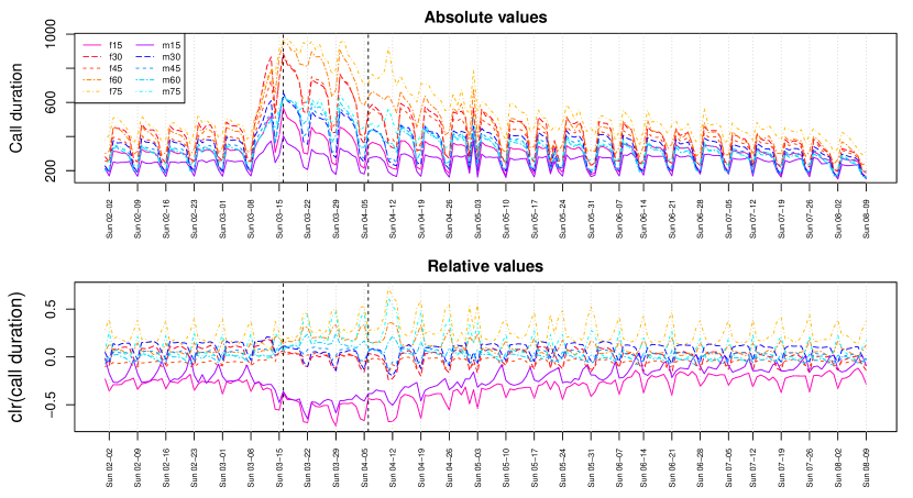
Figure 6: Median values of call durations per gender and age group over time (top), and clr representations separately for female and male age groups (bottom).

Figure 7 presents biplots of a robust PCA for the CLR coefficients for the female (left) and male (right) age groups. The coloring is taken as in the previous biplots, green before lock-down, pink during, purple after lock-down, and light-blue from June 15^th onwards. PC1 explains 72% of the variability for the females, 54% for males, and PC1 and PC2 together explain about 98% variance in both cases. The different groups which are visible in the biplots are essentially weekend-effects or affects due to the lock-down. These grouping effects are essentially caused by the youngest and oldest age groups. When comparing the first observed time period with the last one, we can find quite clear differences in the corresponding PCA scores. These differences are essentially caused by the changing contrasting behavior between the youngest group and the elder groups; groups f75 and m75 (and also m30) do not seem to contribute to this difference. A possible explanation is the exploration of alternative methods for communication, especially for the elder groups.

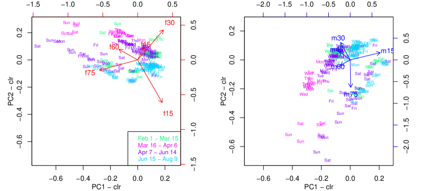
Figure 7: Biplots of the CLR coefficients of the median call duration values for females (left) and male (right) age groups. Green color for the period before the lock-down, pink for lock-down period, light-blue after this period.

3.3 Interactions between source and destination

It can be recorded who is actively calling a person, and who is receiving a call. The former person is called source, and the latter destination. Here we investigate the median ROG values for the different age groups of the females and males. However, the data set is more complex now, because a person from a certain age group can be source, while the destination can originate from a different age group. Moreover, both source and destination will have specific median ROG values.

Figure 8 illustrates these data for four specific cases: source f45 (f45$\_$src) with destination f75 (f75$\_$dst), and source f75 (f75$\_$src) with destination f45 (f45$\_$dst). In both cases, the median ROG values can be taken from the source group or from the destination group, see also figure legend. Throughout the whole period (here from February 1^st - July 26^th), the median ROG values from the source groups (solid lines) have slightly higher values than those of the destination groups (dashed lines) for the same age classes, which can be expected because people from the source groups might call from a place outside their usual environment. While the lines are on a similar level at the beginning and at the end of the considered period, the weekly periodicity changes, probably caused by the summer holidays.

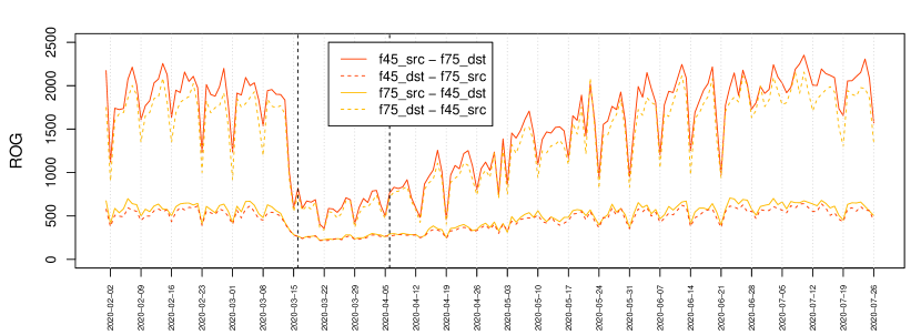
Figure 8: Median ROG values for the female age groups $f45$ and $f75$, depending whether they actively call (src) or they passively receive the call (dst). For example, line f75$\_$src – f45$\_$dst refers to the median ROG values for females in age group f75, actively calling females in age group f45.

In the following analyses we are interested in the similarity of the relative ROG values in terms of correlations, before lock-down (February 1^st – March 15^th) and after (March 16^th – May 31^th). In order to investigate relative information, the CLR coefficients are computed for a composition with all 25 age combinations of the source-destination groups and all 25 age combinations of the destination-source groups, separately for females and males. Figure 9 shows the resulting correlation matrix for the females as a heat map, left for time points before the lock-down, and right after lock-down. The row and column labels are referring to the group numbers. For example, src1-3 refers to the time series f15$\_$src – f30$\_$dst, or dst5-1 is the series f75$\_$dst – f15$\_$src. The heatmaps show that the correlation structure before and after lock-down has clearly changed. Afterwards, there are more blocks with higher (absolute) correlations, and thus more similarity or dissimilarity between certain age groups. In general, there is a more pronounced difference after lock-down in the mobility behavior between the younger and the elder age groups.

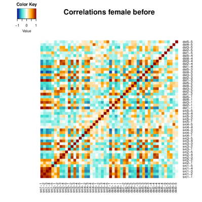
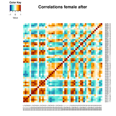
Figure 9: Correlations of the CLR coefficients for median ROG values for the female age groups (1 to 5, referring to 15 to 75$+$), when they are actively calling (src) or passively receiving a call (dst), recorded before March 16^th, 2020 (left), and afterwards (right).

3.4 Incorporating spatial location

The mobile phone data also contain information about the location, in our case about the Austrian political district in which the phone has been used. The Austrian regions had different restrictions during the lock-down phase, and in particular people from all districts in Tirol had the strongest movement restrictions. Thus, in Figure 10 we compare the median ROG values for Kitzbühel, a district in Tirol, and Zell am See, which is also a rural district but located in Salzburg. The absolute values of the female age groups are shown in the upper plots, while the CLR coefficients are presented in the lower plots. Since the same scale is used along the vertical axes, one can clearly see the difference in mobility during the lock-down period in Kitzbühel and Zell am See, and this is also visible in the CLR coefficients. For Kitzbühel, there is much smaller variability of the values during lock-down, and also the relative differences between the age groups become much smaller. The change in the relative differences is not so pronounced for Zell am See. This means that also from a relative point of view, the data structure changes completely in Kitzbühel due to the restrictions.

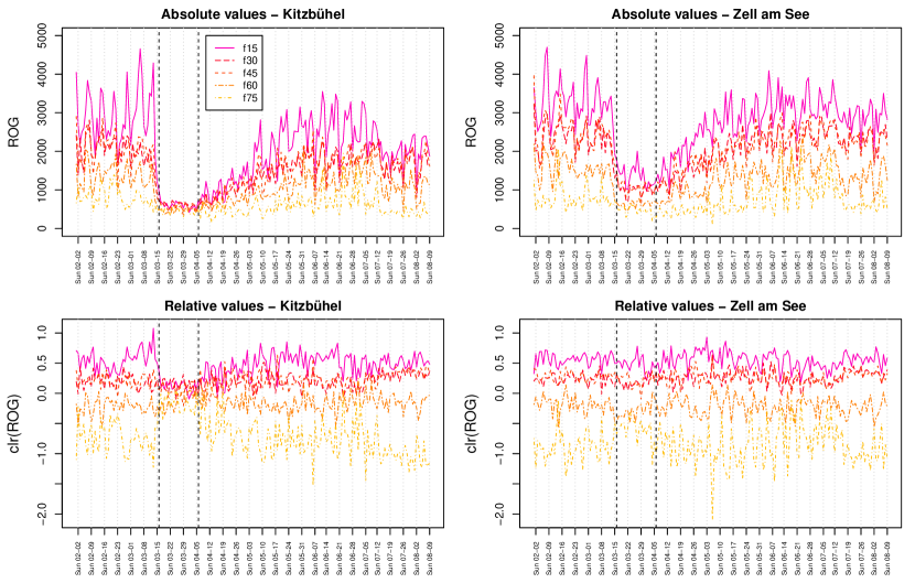
Figure 10: Median ROG values for Kitzbühel (left) and Zell am See (right) as absolute (top) and relative (bottom) information.

Figure 11 focuses on the male age group m30, and compares the composition of all districts in Tirol with that of all districts in Salzburg. The dashed lines refer to the district capitals (Innsbruck and Salzburg, respectively). These districts behave differently compared to the other districts which are rural with many people commuting to their work place. The values of the districts in Tirol (except Innsbruck) get closer to each other after lock-down, and they start to diverge only in the middle of April. This may be explained by a similar mobility behavior of the m30 group within this period, probably caused by home-office or reduced working time. This seems different in districts of Salzburg, where the CLR coefficients show more variability after lock-down.

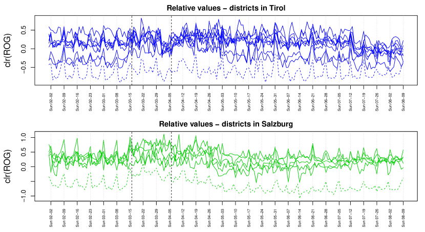
Figure 11: CLR coefficients of median ROG values for the male group m30 in all districts of Tirol (top) and Salzburg (bottom). The capitals are shown as dashed lines.

4 Discussion

By analyzing relative changes using compositional data analysis methodologies formerly hidden insights can be identified. In this work of analyzing mobility during the COVID-19 lock-down measures we see that certain age-groups of the population (elderly, young during weekends) do restrict mobility less than other members of the population. Especially for the elderly which are at high risk of infections potentially additional reminders should be sent to adhere to the interventions. Similarly, for the young groups on weekends additional reminders to use mouth nose protection could be useful.

Declaration of interest

We have no competing interests to declare.

References

- [1] Emanuele Pepe et al. “COVID-19 outbreak response: a first assessment of mobility changes in Italy following national lockdown” In medRxiv, 2020, pp. 2020.03.22.20039933 DOI: 10.1101/2020.03.22.20039933
- [2] Jayson S. Jia et al. “Population flow drives spatio-temporal distribution of COVID-19 in China” In Nature, 2020 DOI: 10.1038/s41586-020-2284-y
- [3] Song Gao et al. “Mobile phone location data reveal the effect and geographic variation of social distancing on the spread of the COVID-19 epidemic”, 2020 arXiv: http://arxiv.org/abs/2004.11430
- [4] Benjamin Jeffrey et al. “Report 24 : Anonymised and aggregated crowd level mobility data from mobile phones suggests that initial compliance with COVID-19 social distancing interventions was high and geographically consistent across the UK”, 2020, pp. 1–19
- [5] Takahiro Yabe et al. “Non-Compulsory Measures Sufficiently Reduced Human Mobility in Japan during the COVID-19 Epidemic”, 2020, pp. 1–9 arXiv: http://arxiv.org/abs/2005.09423
- [6] Michaela A C Vollmer et al. “Report 20 : Using mobility to estimate the transmission intensity of COVID-19 in Italy : A subnational analysis with future scenarios”, 2020
- [7] Bo Xu et al. “Epidemiological data from the COVID-19 outbreak, real-time case information” In Scientific Data 7.1, 2020, pp. 1–6 DOI: 10.1038/s41597-020-0448-0
- [8] SANTAMARIA SERNA Carlos et al. “Measuring the Impact of COVID-19 Confinement Measures on Human Mobility using Mobile Positioning Data (1)” Publications Office of the European Union, 2020 DOI: 10.2760/913067
- [9] IACUS Stefano et al. “How human mobility explains the initial spread of COVID-19 (2)” Publications Office of the European Union, 2020 DOI: 10.2760/61847
- [10] IACUS Stefano et al. “Mapping Mobility Functional Areas ( MFA ) by using Mobile Positioning Data to Inform COVID-19 Policies (3)” Publications Office of the European Union, 2020 DOI: 10.2760/076318
- [11] Thomas Heuzroth “Corona-Pandemie: So hat Ischgl das Virus in die Welt getragen” In WELT URL: https://www.welt.de/wirtschaft/article206879663/Corona-Pandemie-So-hat-Ischgl-das-Virus-in-die-Welt-getragen.html
- [12] Shohin Aheleroff “Customer segmentation for a mobile telecommunications company based on service usage behavior” In Proceedings - 3rd International Conference on Data Mining and Intelligent Information Technology Applications, ICMIA 2011, 2011, pp. 308–313 DOI: 10.5121/ijdkp.2015.5205
- [13] Gokul Chittaranjan, Blom Jan and Daniel Gatica-Perez “Who’s who with big-five: Analyzing and classifying personality traits with smartphones” In Proceedings - International Symposium on Wearable Computers, ISWC, 2011, pp. 29–36 DOI: 10.1109/ISWC.2011.29
- [14] Martin Hillebrand, Imran Khan, Filipa Peleja and Nuria Oliver “MobiSenseUs : Inferring Aggregate Objective and Subjective Well-being from Mobile Data”, 2020
- [15] Hidayet Aksu, Ibrahim Korpeoglu and Özgür Ulusoy “An Analysis of Social Networks Based on Tera-Scale Telecommunication Datasets” In IEEE Transactions on Emerging Topics in Computing 7.2 IEEE Computer Society, 2019, pp. 349–360 DOI: 10.1109/TETC.2016.2627034
- [16] Nour Raeef Al-Molhem, Yasser Rahal and Mustapha Dakkak “Social network analysis in Telecom data” In Journal of Big Data 6.1 SpringerOpen, 2019 DOI: 10.1186/s40537-019-0264-6
- [17] Talayeh Aledavood, Sune Lehmann and Jari Saramäki “Social network differences of chronotypes identified from mobile phone data” In EPJ Data Science 7.1, 2018 DOI: 10.1140/epjds/s13688-018-0174-4
- [18] Ana Nika et al. “Understanding and Predicting Data Hotspots in Cellular Networks” In Mobile Networks and Applications 21.3, 2016, pp. 402–413 DOI: 10.1007/s11036-015-0648-6
- [19] Thi-Nga Dao, Duc Le and Seokhoon Yoon “Predicting Human Location Using Correlated Movements” In Electronics 8.1, 2019, pp. 54 DOI: 10.3390/electronics8010054
- [20] Pengxiang Zhao, Dominik Bucher, Henry Martin and Martin Raubal “A clustering-based framework for understanding individuals’ travel mode choice behavior” In Lecture Notes in Geoinformation and Cartography, 2020, pp. 77–94 DOI: 10.1007/978-3-030-14745-7˙5
- [21] Huan Liu, Lin Ma, Xi Zhao and Jianhua Zou “An Effective Model Between Mobile Phone Usage and P2P Default Behavior” In Lecture Notes in Computer Science (including subseries Lecture Notes in Artificial Intelligence and Lecture Notes in Bioinformatics) 10861 LNCS, 2018, pp. 462–475 DOI: 10.1007/978-3-319-93701-4˙36
- [22] Xavier Andrade, Fabricio Layedra, Carmen Vaca and Eduardo Cruz “RiSC: Quantifying change after natural disasters to estimate infrastructure damage with mobile phone data” In Proceedings - 2018 IEEE International Conference on Big Data, Big Data 2018, 2019, pp. 3383–3391 DOI: 10.1109/BigData.2018.8622374
- [23] Aude Marzuoli and Fengmei Liu “A data-driven impact evaluation of Hurricane Harvey from mobile phone data” In Proceedings - 2018 IEEE International Conference on Big Data, Big Data 2018, 2019, pp. 3442–3451 DOI: 10.1109/BigData.2018.8622641
- [24] Daniel Monsivais et al. “Seasonal and geographical impact on human resting periods” In Scientific Reports 7.1, 2017 DOI: 10.1038/s41598-017-11125-z
- [25] Sibren Isaacman, Vanessa Frias-Martinez and Enrique Frias-Martinez “Modeling human migration paerns during drought conditions in La Guajira, Colombia” In Proceedings of the 1st ACM SIGCAS Conference on Computing and Sustainable Societies, COMPASS 2018, 2018 DOI: 10.1145/3209811.3209861
- [26] Xiaoying Shi et al. “Exploring the Evolutionary Patterns of Urban Activity Areas Based on Origin-Destination Data” In IEEE Access 7, 2019, pp. 20416–20431 DOI: 10.1109/ACCESS.2019.2897070
- [27] Maxime Lenormand et al. “Comparing and modelling land use organization in cities” In Royal Society Open Science 2.12, 2015 DOI: 10.1098/rsos.150449
- [28] Georg Heiler et al. “Country-wide mobility changes observed using mobile phone data during COVID-19 pandemic”, 2020 arXiv: http://arxiv.org/abs/2008.10064
- [29] Jan W. Gooch “Radius of Gyration” In Encyclopedic Dictionary of Polymers New York, NY: Springer New York, 2011, pp. 607–607 DOI: 10.1007/978-1-4419-6247-8˙9741
- [30] Georg Heiler et al. “Behavioral gender differences are reinforced during the COVID-19 crisis” in preparation, 2020
- [31] J. Aitchison “The Statistical Analysis of Compositional Data” Chapman & Hall, London. (Reprinted in 2003 with additional material by The Blackburn Press), 1986
- [32] V. Pawlowsky-Glahn, J.J. Egozcue and R. Tolosana-Delgado “Modeling and Analysis of Compositional Data” Wiley, Chichester, 2015
- [33] Peter Filzmoser, Karel Hron and Matthias Templ “Applied Compositional Data Analysis. With Worked Examples in R” Cham, Switzerland: Springer Series in Statistics, Springer, 2018
- [34] Josh L Espinoza et al. “Applications of weighted association networks applied to compositional data in biology” In Environmental Microbiology Wiley Online Library, 2020
- [35] Thomas P Quinn, Ionas Erb, Mark F Richardson and Tamsyn M Crowley “Understanding sequencing data as compositions: an outlook and review” In Bioinformatics 34.16 Oxford University Press, 2018, pp. 2870–2878
- [36] Huong Thi Trinh, Joanna Morais, Christine Thomas-Agnan and Michel Simioni “Relations between socio-economic factors and nutritional diet in Vietnam from 2004 to 2014: New insights using compositional data analysis” In Statistical methods in medical research 28.8 Sage Publications Sage UK: London, England, 2019, pp. 2305–2325
- [37] Abdennassar Joueid and Germà Coenders “Marketing innovation and new product portfolios. A compositional approach” In Journal of Open Innovation: Technology, Market, and Complexity 4.2 Multidisciplinary Digital Publishing Institute, 2018, pp. 19
- [38] Dorothea Dumuid et al. “Compositional Data Analysis in Time-Use Epidemiology: What, Why, How” In International journal of environmental research and public health 17.7 Multidisciplinary Digital Publishing Institute, 2020, pp. 2220
- [39] John Aitchison and Michael Greenacre “Biplots for compositional data” In Journal of the Royal Statistical Society, Series C (Applied Statistics) 51.4, 2002, pp. 375–392
- [40] M. Hubert, P. J. Rousseeuw and Karlien Vanden Branden “ROBPCA: A New Approach to Robust Principal Component Analysis” In Technometrics 47, 2005, pp. 64–79