DCTRGAN: Improving the Precision of Generative Models with Reweighting

Abstract

Significant advances in deep learning have led to more widely used and precise neural network-based generative models such as Generative Adversarial Networks (Gans). We introduce a post-hoc correction to deep generative models to further improve their fidelity, based on the Deep neural networks using the Classification for Tuning and Reweighting (Dctr) protocol. The correction takes the form of a reweighting function that can be applied to generated examples when making predictions from the simulation. We illustrate this approach using Gans trained on standard multimodal probability densities as well as calorimeter simulations from high energy physics. We show that the weighted Gan examples significantly improve the accuracy of the generated samples without a large loss in statistical power. This approach could be applied to any generative model and is a promising refinement method for high energy physics applications and beyond.

I Introduction

Generative models are a critical component of inference in many areas of science and industry. As a result of recent advances in deep learning, neural network-based generative models are rapidly being deployed to augment slow simulations, act as simulator surrogates, or used for ab initio modeling of data densities directly for inference or for uncertainty quantification. Well-studied methods include Generative Adversarial Networks (Gan) Goodfellow et al. (2014a); Creswell et al. (2018), Variational Autoencoders Kingma and Welling ; Kingma and Welling (2019), and variations of Normalizing Flows Rezende and Mohamed (2015); Kobyzev et al. (2020).

In many industrial applications of generative modeling, the aim is primarily to achieve “realistic” images on a per-example basis. By contrast, in high energy physics applications, the main goal is usually to improve the quality of an ensemble of examples. In other words, it is of paramount importance that the generator accurately reproduce the underlying probability distribution of the training data.

One challenge faced by current generative models is that even though they are able to qualitatively reproduce features of the data probability density, they are often unable to reproduce fine details. While a variety of advanced methods are being proposed to enhance the precision of generative models, we make the observation that a relatively simple operation can be performed on the output of a generative model to improve its fidelity. This operation uses a neural network classifier to learn a weighting function that is applied post-hoc to tweak the learned probability density. The result is a set of weighted examples that can be combined to more accurately model the statistics of interest. This procedure does not improve the fidelity of any particular example, but instead improves the modeling of the probability density.

Estimating probability density ratios with classification has a long history (see e.g., Ref. Hastie et al. (2001); Sugiyama et al. (2012)) and has been used for a wide variety of applications in machine learning research related to generative models Nowozin et al. (2016); Mohamed and Lakshminarayanan (2016); Grover and Ermon (2017); Gretton et al. (2007); Bowman et al. (2015); Lopez-Paz and Oquab (2016); Danihelka et al. (2017); Rosca et al. (2017); Im et al. (2018); Gulrajani et al. (2020); Grover et al. (2017, 2019a); Azadi et al. (2018); Turner et al. (2018); Tao et al. (2018). The most closely related application to this paper is Ref. Grover et al. (2019b) which used learned weights during the training of a generative model to improve fairness. In this work, the weights are derived after the generator is trained. In high energy physics, there are many studies using deep generative models Paganini et al. (2018a, b); Vallecorsa et al. (2019); Chekalina et al. (2018); ATLAS Collaboration (2018); Carminati et al. (2018); Vallecorsa (2018); Musella and Pandolfi (2018); Erdmann et al. (2018, 2019a); de Oliveira et al. (2017a, 2018); Hooberman et al. (2017); Belayneh et al. (2019); Buhmann et al. (2020); de Oliveira et al. (2017b); Butter et al. (2019a); Arjona Martinez et al. (2019); Bellagente et al. (2019); Vallecorsa et al. (2019); Ahdida et al. (2019); Carrazza and Dreyer (2019); Butter et al. (2019b); Lin et al. (2019); Di Sipio et al. (2019); Hashemi et al. (2019); Zhou et al. (2019); Datta et al. (2018); Deja et al. (2019); Derkach et al. (2019); Erbin and Krippendorf (2018); Urban and Pawlowski (2018); Farrell et al. (2019) and using likelihood ratio estimates based on classifiers Andreassen and Nachman (2019); Badiali et al. (2020); Stoye et al. (2018); Hollingsworth and Whiteson (2020); Brehmer et al. (2018a, b, 2020, c); Cranmer et al. (2015); Badiali et al. (2020); Andreassen et al. (2020a, b); Erdmann et al. (2019b); this paper combines both concepts to construct DctrGan, which is a tool with broad applicability in high energy physics and beyond.

This paper is organized as follows. Section II introduces the statistical methods of reweighting and how they can be applied to generative models using deep learning. Numerical results are presented in Sec. III using standard multimodal probability densities as well as calorimeter simulations from high energy physics. The paper ends with conclusions and outlook in Sec. IV.

II Methods

II.1 Generative Models

A generative model $G:\mathbb{R}^{M}\rightarrow\mathbb{R}^{N}$ is a function that maps a latent space (noise) $Z\in\mathbb{R}^{M}$ to a target feature space $X\in\mathbb{R}^{N}$. The goal of the generator is for the learned probability density $p_{G}(x)$ to match the density of a target process $T$, $p_{T}(x)$. There are a variety of approaches for constructing $G$ using flexible parameterizations such as deep neural networks. Some of these methods produce an explicit density estimation for $p_{G}$ and others only allow generation without a corresponding explicit density.

While the method presented in this paper will work for any generative model $G$, our examples will consider the case when $G$ is a Generative Adversarial Network Goodfellow et al. (2014b). A Gan is trained using two neural networks:

$$(G,D) =\operatorname*{argmin}_{G^{\prime}}\operatorname*{argmax}_{D^{\prime}}\Big{(}\mathbb{E}_{X}[\log D^{\prime}(X)]$$

$$\hskip 71.13188pt+\mathbb{E}_{Z}[\log(1-D^{\prime}(G^{\prime}(Z))]\Big{)},$$ (1)

where $D$ is a discriminator/classifier network that distinguishes real examples from those drawn from the generator $G$. The discriminator network provides feedback to the generator through gradient updates and when it is unable to classify examples as drawn from the generator or from the true probability density, then $G$ will be accurate. Gans provide efficient models for generating examples from $G$, but do not generally provide an explicit estimate of the probability density.

This paper describes a method for refining the precision of generative models using a post-processing step that is also based on deep learning using reweighting. A weighting function $W:\mathbb{R}^{N}\rightarrow[0,\infty)$ is a map designed so that $p_{G}(x)W(x)\approx p_{T}(x)$. Augmenting a generator with a reweighting function will not change the fidelity of any particular example, but it will improve the relative density of examples. Therefore, this method is most useful for applications that use generators for estimating the ensemble properties of a generative process and not the fidelity of any single example. For example, generators trained to replace or augment slow physics-based simulators may benefit from the addition of a reweighting function. Such generators have been proposed for a variety of tasks in high energy physics and cosmology Paganini et al. (2018a, b); Vallecorsa et al. (2019); Chekalina et al. (2018); ATLAS Collaboration (2018); Carminati et al. (2018); Vallecorsa (2018); Musella and Pandolfi (2018); Erdmann et al. (2018, 2019a); de Oliveira et al. (2017a, 2018); Hooberman et al. (2017); Belayneh et al. (2019); Buhmann et al. (2020); de Oliveira et al. (2017b); Butter et al. (2019a); Arjona Martinez et al. (2019); Bellagente et al. (2019); Vallecorsa et al. (2019); Ahdida et al. (2019); Carrazza and Dreyer (2019); Butter et al. (2019b); Lin et al. (2019); Di Sipio et al. (2019); Hashemi et al. (2019); Zhou et al. (2019); Datta et al. (2018); Deja et al. (2019); Derkach et al. (2019); Erbin and Krippendorf (2018); Urban and Pawlowski (2018); Farrell et al. (2019).

II.2 Statistical Properties of Weighted Examples

Let $G$ be a trained generative model that is designed to mimic the target process $T$. Furthermore, let $W(X)$ be a random variable that corresponds to weights for each value of $X$. If $f$ is a function of the phase space $X$, one can compute the weighted expectation value

$$\mathbb{E}[f(X),W(X)] =\int p(x)\,W(x)\,f(x)\,dx\,.$$ (2)

Nearly every use of Monte Carlo event generators in high energy physics can be cast in the form Eq. 2. A common use-case is the estimation of the bin counts of a histogram, in which case $f$ is an indicator function that is one if $x$ is in the bin and zero otherwise. For the true expectation value, $p(x)\mapsto p_{T}(x)$ and $W(x)\mapsto 1$ , while for the nominal generator approximation, $p(x)\mapsto p_{G}(x)$ with $W(x)$ still unity. The goal of DctrGan is to learn a weighting function $W$ that reduces the difference between $\mathbb{E}_{T}[f(X)]$ and $\mathbb{E}_{G}[f(X),W(X)]$ for all functions $f$. The ideal function that achieves this goal is

$$W(x)={p_{T}(x)\over p_{G}(x)}\,.$$ (3)

Before discussing strategies for learning $W$, it is important to examine the sampling properties of weighted examples. To simplify the discussion in the remainder of this subsection, we will assume that the ideal reweighting function $W$ has been learned exactly, so that

$$\bar{f}=\mathbb{E}_{T}[f(X)]=\mathbb{E}_{G}[f(X),W(X)]\,.$$ (4)

for every observable $f$. In practice, small deviations from the ideal reweighting function will result in subleading contributions to the statistical uncertainty.

Now suppose we generate events $x_{i}^{G}$, $i=1,\dots,N_{G}$, and there are truth events $x_{i}^{T}$, $i=1,\dots,N_{T}$. We are interested in how large $N_{G}$ must be in order to achieve the same statistical precision as the truth sample. The key observation we will make is that the required $N_{G}$ depends jointly on the observable $f$ and the weights $W$.

Since we will be interested in variances, it makes sense to consider the mean-subtracted observable

$$\delta f=f-\bar{f}\,.$$ (5)

The sampling estimates for $\mathbb{E}_{T}[\delta f(X)]$ and $\mathbb{E}_{G}[\delta f(X),W(X)]$ are

$$\begin{aligned} &\mathbb{\hat{E}}_{T}[\delta f(X)]={1\over N_{T}}\sum_{i=1}^{N_{T}}\delta f(x_{i}^{T})\\ &\mathbb{\hat{E}}_{G}[\delta f(X),W(X)]={1\over N_{G}}\sum_{i=1}^{N_{G}}W(x_{i}^{G})\delta f(x_{i}^{G})\,,\end{aligned}$$ (6)

where hats denote sampling estimates of expectation values. The variances of the sampling estimates are given by

$$\begin{aligned} \text{Var}_{T}[\mathbb{\hat{E}}_{T}[\delta f(X)]]&={1\over N_{T}}\text{Var}_{T}[\delta f(X)]\\ &={1\over N_{T}}\int dx\,p_{T}(x)\delta f(x)^{2}\,,\end{aligned}$$ (7)

and

$$\begin{aligned} &\text{Var}_{G}[\mathbb{\hat{E}}_{G}[\delta f(X),W(X)]]={1\over N_{G}}\text{Var}_{G}[W(X)\delta f(X)]\\ &\qquad\qquad\qquad={1\over N_{G}}\int dx\,p_{G}(x)W(x)^{2}\delta f(x)^{2}\\ &\qquad\qquad\qquad={1\over N_{G}}\int dx\,p_{T}(x)W(x)\delta f(x)^{2}\,.\end{aligned}$$ (8)

Equating Eq. 7 and LABEL:eq:varG, we see that to achieve the same statistical precision as the truth events for a given observable $f$, we need to generate

$$N_{G}=N_{T}\times{\int dx\,p_{T}(x)W(x)\delta f(x)^{2}\over\int dx\,p_{T}(x)\delta f(x)^{2}}\,$$ (9)

number of events. How many events we need depends on the observable $f$ and the weights $W$. If $W=1$ everywhere (the generator exactly learns $T$), then $N_{G}=N_{T}$ for every observable, as expected. Otherwise, if the weights are small (large) in the parts of phase space preferred by $\delta f$, then we will need less (more) events than $N_{T}$. Smaller weights are better for statistical power – they correspond to regions of phase space which are over-represented by the generator.

One cannot simply reduce the error everywhere by making all of the weights small. If the weights are small somewhere in phase space, they must be large somewhere else. To see this, observe that with the ideal reweighting function, in the large $N$ limit, the weights are automatically normalized across the entire sample such that they sum to $N_{G}$:

$$\begin{aligned} \sum_{i=1}^{N_{G}}W(x_{i}^{G})&\to N_{G}\int dx\,p_{G}(x)W(x)=N_{G}\,,\\ \end{aligned}$$ (10)

where in the last equation we have substituted Eq. 3. So indeed the weights cannot be small everywhere in phase space.

Evidently, if we want the generator to have good statistical precision across a wide range of observables, we want the weights to be close to unity. Otherwise, there will always be some observables for which we need to generate many more events than $N_{T}$.

As a special case of Eq. 9, consider that $f(x)$ is a histogram bin function, specifically that it is one in a neighborhood of $x=x_{0}$ and zero otherwise. For a sufficiently small neighborhood, we can ignore the mean $\bar{f}$ (it is proportional to the volume of the neighborhood), and (9) reduces to

$$N_{G}=N_{T}W(x_{0})\,.$$ (11)

In other words, the value of the weight in the histogram bin directly determines how many events we need to generate to achieve the same statistical precision as the truth sample.

Finally, while the integral formulas above are formally correct and lead to various insights, they are of limited practical usefulness since we generally do not know $p_{T}(x)$ and $p_{G}(x)$ and cannot evaluate the integrals over $x$. For actually estimating the uncertainties on expected values, one should replace the integrals in Eq. 7 and Eq. LABEL:eq:varG with their sampling estimates.

II.3 Learning the Weighting Function

The weighting function $W$ is constructed using the Deep neural networks using Classification for Tuning and Reweighting (Dctr) methodology Andreassen and Nachman (2019) (see also Ref. Badiali et al. (2020); Stoye et al. (2018); Hollingsworth and Whiteson (2020); Brehmer et al. (2018a, b, 2020, c); Cranmer et al. (2015); Badiali et al. (2020); Andreassen et al. (2020a, b)). Let $\mathcal{X}_{\text{real}}$ be a set of examples drawn from $p_{X}(x)$ and $\mathcal{X}_{\text{fake}}$ be a set of examples drawn from $p_{Z}(z)$ and then mapped through $G$, henceforth called $p_{G}(x)$ for $x=G(z)$. A neural network classifier $h:\mathbb{R}^{N}\rightarrow[0,1]$ is trained to distinguish $\mathcal{X}_{\text{real}}$ from $\mathcal{X}_{\text{fake}}$ using the binary cross entropy loss function so that $h(x)=1$ corresponds to $\mathcal{X}_{\text{real}}$ . The weighting function is then constructed as $W(x)=h(x)/(1-h(x))$. With sufficient training data, classifier expressiveness, and training flexibility, one can show that $W$ approaches the likelihood ratio $p_{T}(x)/p_{G}(x)$. If the weights are exactly the likelihood ratio, then the expectation values computed in Eq. 2 will be unbiased.

Training a classifier is often easier and more reliable than training a full generative model. Therefore, a natural question is why learn $G$ at all? The answer is because the further $W(x)$ is from the constant unity function, the more statistical dilution will arise from the generated examples (when a sufficiently broad range of observables is considered), as described in Sec. II.2. In particular, this method does not work at all when there are weights that are infinite, corresponding to regions of phase space where $p_{T}(x)>0$ but $p_{G}(x)=0$. Therefore, the Dctr approach should be viewed as a refinement and the better $G$ is to begin with, the more effective $W$ will be in refining the density. Our method differs from the refinement proposed in Ref. Erdmann et al. (2018) because Dctr-ing leaves the data-points intact and only changes their statistical weight while Erdmann et al. (2018) modifies the data-points themselves. A combined framework that simultaneously changes both data and weights might be an interesting avenue for future studies.

III Results

The DctrGan approach is illustrated with two sets of examples: one set where the true density $p_{T}$ is known analytically (Sec. III.1) and one where $p_{T}$ is not known, but samples can be drawn from it (Sec. III.2).

III.1 Multimodel Gaussian Distributions

As a first set of examples, Gaussian mixture models are simulated in one and two dimensions. Multimodal probability densities are traditionally challenging for standard Gans to model precisely and are a useful benchmark for the DctrGan methodology. In particular, the following random variables are simulated:

1. 1D bimodal:

   $$p_{X}(x)=\frac{1}{2}N(x,-1,0.4)+\frac{1}{2}N(x,1,0.4),$$ (12)

   where $N(x,\mu,\sigma)$ is the probability density of a normal random variable with mean $\mu$ and standard deviation $\sigma$ evaluated at $x$.

2. 2D circular:

   $$p_{X}(x) =\frac{1}{8}\sum_{i=1}^{8}\left[N\left(x_{0},\cos\left(\frac{2\pi i}{8}\right),0.1\right)\right.$$

   $$\hskip 42.67912pt\times\left.N\left(x_{1},\sin\left(\frac{2\pi i}{8}\right),0.1\right)\right],$$ (13)

   where $x=(x_{0},x_{1})\in\mathbb{R}^{2}$.

3. 2D $5\times 5$ grid:

   $$p_{X}(x) =\frac{1}{25}\sum_{i=1}^{5}\sum_{j=1}^{5}\left[N\left(x_{0},\left(i+0.1\right),0.1\right)\right.$$

   $$\hskip 71.13188pt\times\left.N\left(x_{1},j+0.1,0.1\right)\right].$$ (14)

All models were implemented in Keras Chollet (2017) with the Tensorflow backend Abadi et al. (2016) and optimized with the Adam Kingma and Ba (2014). The discriminator $D$ networks have two hidden layers with 25 nodes each and use the rectified linear unit (ReLU) activation function. The sigmoid function is used after the last layer. The generator networks $G$ also has two hidden layers, with 15 units each. A latent space of dimension 5, 8, and 25 is used for the 1D bimodal, 2D circular, and 2D $5\times 5$ grid, respectively. Each model was trained with a batch size of 128 for 10,000 epochs (passes through the batches, not the entire dataset). For the reweighting model, three hidden layers were used for all three cases with ReLU activiations on the intermeidate layers and a sigmoid for the last layer. For the 2D models, the numbers of hidden units were 64, 128, and 256 while the 1D example used 20 hidden notes on each intermediate layer. The binary cross entropy was used for the loss function and the models were trained for 100 epochs (passes through the entire dataset).

The resulting probability densities are presented in Fig. 1. In all cases, the fidelity of the Gan density is significantly improved using reweighting.

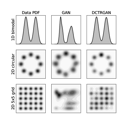
Figure 1: Three multi-modal Gaussian examples. The true probability density $p_{X}$ is shown in the first column, a Gan density is presented in the second column, and then the density from DctrGan is drawn in the third column. Examples inspired from Ref. Fisher et al. (2018).

III.2 Calorimeter Simulation Examples

Data analysis in high energy physics makes extensive use of simulations for inferring fundamental properties of nature. These complex simulations encode physics spanning a vast energy range. The most computationally demanding part of the simulation stack is the modeling of particles stopping in the dense material of calorimeters that part of most detectors. Gans have been investigated as a surrogate model for accelerating these slow calorimeter simulations Paganini et al. (2018a, b); Vallecorsa et al. (2019); Chekalina et al. (2018); ATLAS Collaboration (2018); Carminati et al. (2018); Vallecorsa (2018); Musella and Pandolfi (2018); Erdmann et al. (2018, 2019a); de Oliveira et al. (2017a, 2018); Hooberman et al. (2017); Belayneh et al. (2019); Buhmann et al. (2020)

The Gan model studied here is a modified version of the Bounded-Information-Bottleneck autoencoder (BIB-AE) Voloshynovskiy et al. (2019) shown in Ref. Buhmann et al. (2020). The BIB-AE setup is based on the encoder-decoder structure of a VAE, but its training is enhanced through the use of Wasserstein-Gan Arjovsky et al. (2017)-like critics. The theoretical basis of the model is discussed in Ref. Voloshynovskiy et al. (2019), while the explicit architecture and training process is described in the appendix of Ref. Buhmann et al. (2020). The main modification to Ref. Buhmann et al. (2020) is introduced to reduce mode collapse: regions of phase space that are significantly under- or over-sampled from the Gan. If extreme enough, such regions can cause Dctr weights that lead to infinites in the loss function. Our modified version maintains the encoder and decoder architecture, but each critic is replaced by a set of two identical critic networks. These two critics are trained in parallel, however one of the two has its weights reset after every epoch. Based on its training history the continuously trained critic may be blind to certain artifacts in the generated shower images that lead to mode collapse. The reset critic, however, is able to notice and reduce such artifacts. Additionally we change the input noise to be uniform instead of Gaussian and skip the neural network based post processing described in Ref. Buhmann et al. (2020), as most of its effects can be replicated through the Dctr approach.

The real examples $T$ are based on detailed detector simulations using Geant4 10.4 Agostinelli et al. (2003) through a DD4hep 1.11 Frank et al. (2014) implementation of the International Large Detector (ILD) Abramowicz et al. (2020) proposed for the International Linear Collider. The calorimeter is composed of 30 active silicon layers with tungsten absorber. The energy recorded in each layer is projected onto a regular grid of $30\times 30$ cells. To simulate the ILD Minimal Ionizing Particle (MIP) cutoff we removes hits with energies $<0.1~{}\text{MeV}$ for both the Geant4 and Gan showers. All showers are generated for an incident photon with an energy of 50 GeV. More details on the simulation are given in Ref. Buhmann et al. (2020).

Two different Dctr models are trained: one using the original data dimensionality (low-level or LL) and one that uses slightly processed inputs with lower dimensionality. The latter network is built from 33 features: the number of non-zero cells, the longitudinal centroid (energy-weighted layer index of the shower: $\sum_{i=1}^{30}i\,E_{i}/\sum_{i=1}^{30}E_{i}$), the total energy, and the energy in each of the thirty layers. A fully connected network processes these observables, with two hidden layers of 128 nodes each. The ReLU activation is used for the intermediate layers and the sigmoid is used for the final layer and the model is trained with the binary cross entropy loss function. The network was implemented using Keras with the Tensorflow backend and optimized with the Adam and optimized with a batch size of 128 for 50 epochs.

The low-level classifier was trained directly on the $30\times 30\times 30$ shower images. On major problem in this approach are artificial features in the Gan showers caused by mode collapse. These give the classifier a way to distinguish between Geant4 and Gan without learning the actual physics. This in turn means that the showers with a high classification score are not necessarily the most realistic ones, which reduces the effectiveness of the reweighting. Therefore a large part of the low-level classifier setup is designed to reduce the impact of such artifacts. The feature processing for the high-level network acts as an effective regularization that mitigates these effects.

The low-level classifier was built using PyTorch Paszke et al. (2019). The initial $30\times 30\times 30$ input image first has a 50% chance of being flipped along the $x$ direction and another 50% chance of being flipped along the $y$ direction. These directions are perpendicular to the longitudinal direction of the incoming photon. The input is largely symmetric under these transformations, but they make it harder for the classifier to pick up on the above mentioned artifacts. The image is then passed through 3 layers of 3D-convolutions, all with 128 output filters and $3\times 3\times 3$ size kernels. The first two convolutions have a stride of 2 with a zero padding of 1, while the third has a stride of 1 and no padding. Between the first and second and second and third convolution layer-norm steps are performed. The $128\times 6\times 6\times 6$ output of the final convolutions is flattened and passed to a set of fully connected layers with (64, 256, 256, 1) output nodes, respectively. Each layer uses a LeakyReLU activation function Maas et al. (2013) with a slope of 0.01, except for the final output layer, which uses a sigmoid activation. The network is trained with a binary cross entropy loss function using the Adam optimizer with a learning rate of $10^{-3}$. The training set consist of 500k Gan showers and 177k Geant4 showers, the Geant4 set is tiled, so it matches the size of the Gan set. This is equivalent to increasing the training weights of the Geant4 set, but was found to converge better than using weights. The network is trained for 1 epoch, as longer training makes the classifier more sensitive to the artificial structures in the Gan showers. After training the classifier is calibrated using Temperature Scaling Guo et al. (2017). Finally we clip the individual per shower weight to be no larger than 5.

Figure 2 shows histograms of the learned Dctr weights for both the low-level and high-level models. The most probable weight is near unity, with a long and asymmetric tail towards low weights. The right plot of Fig. 2 shows that there is a positive correlation between the weights of the two models.

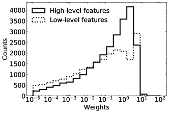
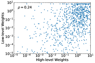
Figure 2: The weights of the low-level and high-level Dctr models. The top plot presents histograms of the weights and the bottom plot presents a scatter plot demonstrating the correlation between the weights of the two models. The Pearson correlation ($\rho$) is indicated in the plot.

Figures 3-6 show histograms of various one-dimensional observables from the full $30\times 30\times 30$-dimensional space. In each plot, two metrics are computed in order to quantify the performance of the generative models. First, the distance measure

$$\langle S^{2}\rangle=\frac{1}{2}\sum_{i=1}^{n_{\text{bins}}}\frac{(h_{1,i}-h_{2,i})^{2}}{h_{1,i}+h_{2,i}}\,,$$ (15)

is used to quantify how similar the Gan histograms are to the Geant4 ones. This measure known in the information theory literature as triangular discrimination Topsoe (2000) (and is an $f$-divergence similar to the $\chi^{2}$ divergence Nachman (2016)). In the high-energy physics literature, this is often called the separation power Hocker et al. (2007). It has the property that it is $0$ if the two histograms are the same and 1 when they are non-overlapping in every bin. As described in Sec. II.2, the tradeoff for improved performance is statistical dilution. To quantify this dilution, the uncertainty on the mean of the observable using the Gan is computed divided by the uncertainty computed using Geant4, denoted $r$ (see Section II.2 for a detailed discussion of these uncertainties). Since the Gan and Geant4 datasets have the same number of events, $r\sim 1$ without Dctr and deviates from one for the weighted Gan models. The effective number of events contained in a weighted sample is observable-dependent, but $r^{2}$ is approximately by the ratio of the effective number of events in the Geant4 dataset to the Gan one. These values are typically between 1-10 while the Gan is many ten-thousand times faster than Geant4 Buhmann et al. (2020).

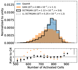
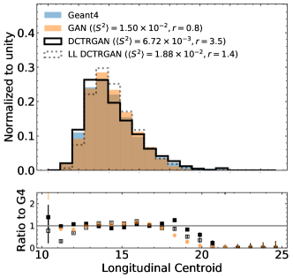
Figure 3: Histograms of various observables from simulated calorimeter showers of 50 GeV photons in a 5-layer calorimeter with $30\times 30$ cells in each layer. A cell is activated if a non-zero energy is registered in that cell. The panels below each histogram show the ratio between the Gan or the DctrGan and the physics-based simulator Geant4. The legend includes the separation power $\langle S^{2}\rangle$ between the (weighted) Gan model and the Geant4 model. Additionally, the ratio $r$ of the uncertainty in the mean of the observable between the Gan and Geant4 is also presented.

Three composite observables are presented in Fig. 3. The total number of activated cells is more peaked around 780 in Geant4 than the Gan and both the low-level and high-level models are able to significantly improve the agreement with Geant4. The value of $\langle S^{2}\rangle$ is about 20 times smaller than the unweighted Gan for the high-level Dctr model and about 5 times smaller for the low-level model. The statistical dilution is modest for the low-level model with $r=1.2$ while it is 3.6 for the high-level model. The modeling of the total energy is also improved through the reweighting, where both the low-level and high-level models shift the energy towards lower values. The longitudinal centroid is already relatively well-modeled by the Gan, but is further improved by the high-level Dctr model, reducing the $\langle S^{2}\rangle$ by more than a factor of two.

Histograms of the energy in representative layers are shown in Fig. 4. Generally, the Geant4 showers penetrate deeper into the calorimeter than the Gan showers, so the energy in the early layers is too high for the Gan and the energy in the later layers is too low. The Dctr models are able to correct these trends, with a systematically superior fidelity as measured by $\langle S^{2}\rangle$ for the high-level model.

The modeling of correlations between layers is probed in Fig. 5 by examining histograms of the difference between energies in different layers. Layers that are closer together should be more correlated. This manifests as histograms with a smaller spread for layers that are physically closer together. For layers that intercept the shower before its maximum, the difference in energy between a layer and the next layer is negative. The shower maximum is typically just beyond the tenth layer. The fidelity improvements from the weighting in the difference histograms is comparable to the per-layer energy histograms from Fig. 4. Interestingly, in cases when the $\langle S^{2}\rangle$ for the Gan is already good without weighting (e.g. the energy in layer 15 - layer 16), the modeling still improves with the Dctr approach and there can still be significant statistical dilution.

Another way to visualize correlations in the data is to compute the linear correlation coefficient between observables. This is reported for a representative set of observables in Fig. 7. Generally, the difference in correlations between the Gan and Geant4 are improved after applying the Dctr reweighting, with many of the residual differences reducing by factors of about 2-10.

Figures 3-5 are features that were directly used by the high-level model. Figure 6 presents histograms for a collection of observables that were not accessible to the high-level model during training. In particular, the energy-weighted second moment along the $x$-direction are computed for each layer. The results for the $y$-direction are nearly the same. Despite not being present during training, the high-level network is still able to improve the the performance over the unweighted Gan in every case with only a modest reduction in statistical power. Weights in the Dctr models are per-example so one can compute any observable even if they are not explicitly part of the reweighting model evaluation.

A summary of the overall performance appears in Fig. 8. The most probable ratio of $\langle S^{2}\rangle$ computed with DctrGan to the one computed with the unweighted Gan is between 0.4 and 0.5 and most most of the observables show improvement after weighting. As mentioned earlier, the Gan and Geant4 datasets have the same number of events so $r\sim 1$ without Dctr. For the low-level model, $r$ has a narrow distribution peaked at about 1.5. In contrast, the high-level model is peaked past two with a tail out to around 5. This difference in $r$ and the overall performance between the low- and high-level models is in part from the extensive regularization of the low-level model during training. The high-level model is also highly-regularized by the dimensionality reduction, but otherwise has a sufficiently complex classifier that is not arrested during training.

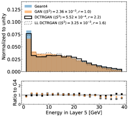
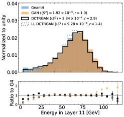
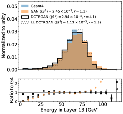
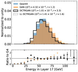
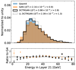
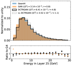
Figure 4: Histograms of total energies in selected layers of the calorimeter. The panels below each histogram show the ratio between the Gan or the DctrGan and the physics-based simulator Geant4. The legend includes the separation power $\langle S^{2}\rangle$ between the (weighted) Gan model and the Geant4 model. Additionally, the ratio $r$ of the uncertainty in the mean of the observable between the Gan and Geant4 is also presented. Underflow and overflow are not included in the leftmost or rightmost bins.

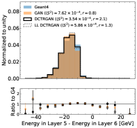
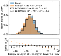
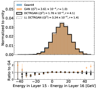
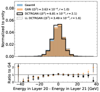
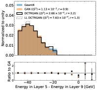
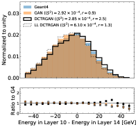
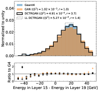
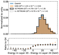
Figure 5: Selected histograms of total energies differences between layer 5 (left), 10 (second), 15 (third), an 20 (right) with the layer that is one later (top) and four later (bottom). The panels below each histogram show the ratio between the Gan or the DctrGan and the physics-based simulator Geant4. The legend includes the separation power $\langle S^{2}\rangle$ between the (weighted) Gan model and the Geant4 model. Additionally, the ratio $r$ of the uncertainty in the mean of the observable between the Gan and Geant4 is also presented. Underflow and overflow are not included in the leftmost or rightmost bins.

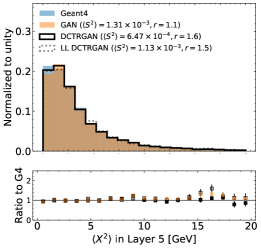
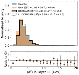
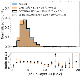
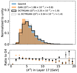
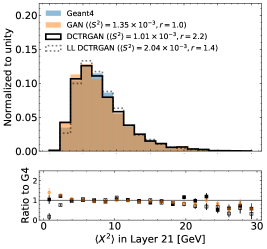
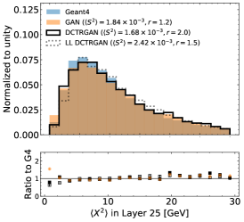
Figure 6: Histograms of energy weighted second moment in per layer. The panels below each histogram show the ratio between the Gan or the DctrGan and the physics-based simulator Geant4. The legend includes the separation power $\langle S^{2}\rangle$ between the (weighted) Gan model and the Geant4 model. Additionally, the ratio $r$ of the uncertainty in the mean of the observable between the Gan and Geant4 is also presented. Underflow and overflow are not included in the leftmost or rightmost bins.

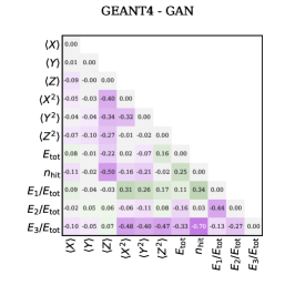
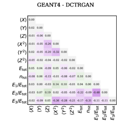
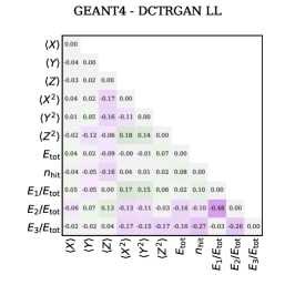
Figure 7: Differnces in pairwise linear correlations between the stated observables between Geant4 and the nominal Gan (left), for the high-level DctrGan (middle) and the low-level DctrGan (right). Darker colors indicate stronger correlation.

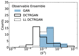
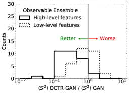
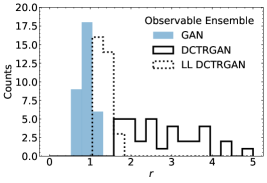
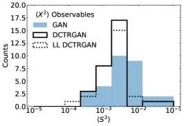
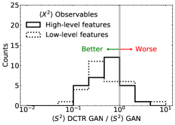
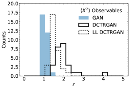
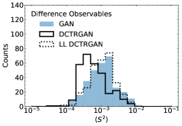
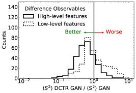
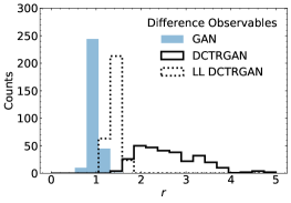
Figure 8: Histograms that summarize the performance of the reweighting models. The first column presents histograms of $\langle S^{2}\rangle$ for all of the observables shown in the previous figures and the second column shows the ratio of $\langle S^{2}\rangle$ for the Gan compared with the DctrGan models. The third column quantifies the statistical dilution using $r$. The top row includes all of the 33 input features to the high-level network, the second row includes all 30 $\langle X^{2}\rangle$ observables, and the third row includes all differences between layers.

IV Conclusions and Outlook

This paper has introduced a post-processing method for generative models to improve their accuracy. While the focus lies on deep generative models, it could similarly be used to enhance the precision of other fast simulation tools (such as Delphes de Favereau et al. (2014)). The approach is based on reweighting and the result is a combined generator and weighting function that produces weighted examples. These weighted examples can be used to perform inference using the same tools as for unweighted events. The potential of deep generative models continues to expand as their fidelity improves and tools like DctrGan may be able help achieve the target precision for a variety of applications.

Code and Data

The code for this paper can be found at https://github.com/bnachman/DCTRGAN. Examples and instructions to reproduce the calorimeter GAN dataset are available at https://github.com/FLC-QU-hep/getting_high.

References

- Goodfellow et al. (2014a) I. J. Goodfellow et al., Generative Adversarial Nets, Conference on Neural Information Processing Systems 2, 2672 (2014a).
- Creswell et al. (2018) A. Creswell, T. White, V. Dumoulin, K. Arulkumaran, B. Sengupta, and A. A. Bharath, Generative adversarial networks: An overview, IEEE Signal Processing Magazine 35, 53 (2018).
- (3) D. P. Kingma and M. Welling, International Conference on Learning Representations arXiv:1312.6114 [stat.ML] .
- Kingma and Welling (2019) D. P. Kingma and M. Welling, An Introduction to Variational Autoencoders, Foundations and Trends in Machine Learning 12, 307 (2019).
- Rezende and Mohamed (2015) D. J. Rezende and S. Mohamed, Variational inference with normalizing flows, International Conference on Machine Learning 37, 1530 (2015).
- Kobyzev et al. (2020) I. Kobyzev, S. Prince, and M. Brubaker, Normalizing Flows: An Introduction and Review of Current Methods, IEEE Transactions on Pattern Analysis and Machine Intelligence , 1 (2020).
- Hastie et al. (2001) T. Hastie, R. Tibshirani, and J. Friedman, The Elements of Statistical Learning, Springer Series in Statistics (Springer New York Inc., New York, NY, USA, 2001).
- Sugiyama et al. (2012) M. Sugiyama, T. Suzuki, and T. Kanamori, Density Ratio Estimation in Machine Learning (Cambridge University Press, 2012).
- Nowozin et al. (2016) S. Nowozin, B. Cseke, and R. Tomioka, F-gan: Training generative neural samplers using variational divergence minimization, in Proceedings of the 30th International Conference on Neural Information Processing Systems, NIPS’16 (Curran Associates Inc., Red Hook, NY, USA, 2016) p. 271–279.
- Mohamed and Lakshminarayanan (2016) S. Mohamed and B. Lakshminarayanan, Learning in implicit generative models (2016), arXiv:1610.03483 [stat.ML] .
- Grover and Ermon (2017) A. Grover and S. Ermon, Boosted generative models (2017), arXiv:1702.08484 [cs.LG] .
- Gretton et al. (2007) A. Gretton, K. Borgwardt, M. Rasch, B. Schölkopf, and A. J. Smola, A kernel method for the two-sample-problem, in Advances in Neural Information Processing Systems 19, edited by B. Schölkopf, J. C. Platt, and T. Hoffman (MIT Press, 2007) pp. 513–520.
- Bowman et al. (2015) S. R. Bowman, L. Vilnis, O. Vinyals, A. M. Dai, R. Jozefowicz, and S. Bengio, Generating sentences from a continuous space (2015), arXiv:1511.06349 [cs.LG] .
- Lopez-Paz and Oquab (2016) D. Lopez-Paz and M. Oquab, Revisiting classifier two-sample tests (2016), arXiv:1610.06545 [stat.ML] .
- Danihelka et al. (2017) I. Danihelka, B. Lakshminarayanan, B. Uria, D. Wierstra, and P. Dayan, Comparison of maximum likelihood and gan-based training of real nvps (2017), arXiv:1705.05263 [cs.LG] .
- Rosca et al. (2017) M. Rosca, B. Lakshminarayanan, D. Warde-Farley, and S. Mohamed, Variational approaches for auto-encoding generative adversarial networks (2017), arXiv:1706.04987 [stat.ML] .
- Im et al. (2018) D. J. Im, H. Ma, G. Taylor, and K. Branson, Quantitatively evaluating gans with divergences proposed for training (2018), arXiv:1803.01045 [cs.LG] .
- Gulrajani et al. (2020) I. Gulrajani, C. Raffel, and L. Metz, Towards gan benchmarks which require generalization (2020), arXiv:2001.03653 [cs.LG] .
- Grover et al. (2017) A. Grover, M. Dhar, and S. Ermon, Flow-gan: Combining maximum likelihood and adversarial learning in generative models (2017), arXiv:1705.08868 [cs.LG] .
- Grover et al. (2019a) A. Grover, J. Song, A. Agarwal, K. Tran, A. Kapoor, E. Horvitz, and S. Ermon, Bias correction of learned generative models using likelihood-free importance weighting (2019a), arXiv:1906.09531 [stat.ML] .
- Azadi et al. (2018) S. Azadi, C. Olsson, T. Darrell, I. Goodfellow, and A. Odena, Discriminator rejection sampling (2018), arXiv:1810.06758 [stat.ML] .
- Turner et al. (2018) R. Turner, J. Hung, E. Frank, Y. Saatci, and J. Yosinski, Metropolis-hastings generative adversarial networks (2018), arXiv:1811.11357 [stat.ML] .
- Tao et al. (2018) C. Tao, L. Chen, R. Henao, J. Feng, and L. C. Duke, Chi-square generative adversarial network, in Proceedings of the 35th International Conference on Machine Learning, Proceedings of Machine Learning Research, Vol. 80, edited by J. Dy and A. Krause (PMLR, Stockholmsmässan, Stockholm Sweden, 2018) pp. 4887–4896.
- Grover et al. (2019b) A. Grover, K. Choi, R. Shu, and S. Ermon, Fair generative modeling via weak supervision., CoRR abs/1910.12008 (2019b).
- Paganini et al. (2018a) M. Paganini, L. de Oliveira, and B. Nachman, Accelerating Science with Generative Adversarial Networks: An Application to 3D Particle Showers in Multilayer Calorimeters, Phys. Rev. Lett. 120, 042003 (2018a), arXiv:1705.02355 [hep-ex] .
- Paganini et al. (2018b) M. Paganini, L. de Oliveira, and B. Nachman, CaloGAN : Simulating 3D high energy particle showers in multilayer electromagnetic calorimeters with generative adversarial networks, Phys. Rev. D97, 014021 (2018b), arXiv:1712.10321 [hep-ex] .
- Vallecorsa et al. (2019) S. Vallecorsa, F. Carminati, and G. Khattak, 3D convolutional GAN for fast simulation, Proceedings, 23rd International Conference on Computing in High Energy and Nuclear Physics (CHEP 2018): Sofia, Bulgaria, July 9-13, 2018 214, 02010 (2019).
- Chekalina et al. (2018) V. Chekalina, E. Orlova, F. Ratnikov, D. Ulyanov, A. Ustyuzhanin, and E. Zakharov, Generative Models for Fast Calorimeter Simulation, in 23rd International Conference on Computing in High Energy and Nuclear Physics (CHEP 2018) Sofia, Bulgaria, July 9-13, 2018 (2018) arXiv:1812.01319 [physics.data-an] .
- ATLAS Collaboration (2018) ATLAS Collaboration, Deep generative models for fast shower simulation in ATLAS, ATL-SOFT-PUB-2018-001 (2018).
- Carminati et al. (2018) F. Carminati, A. Gheata, G. Khattak, P. Mendez Lorenzo, S. Sharan, and S. Vallecorsa, Three dimensional Generative Adversarial Networks for fast simulation, Proceedings, 18th International Workshop on Advanced Computing and Analysis Techniques in Physics Research (ACAT 2017): Seattle, WA, USA, August 21-25, 2017, J. Phys. Conf. Ser. 1085, 032016 (2018).
- Vallecorsa (2018) S. Vallecorsa, Generative models for fast simulation, Proceedings, 18th International Workshop on Advanced Computing and Analysis Techniques in Physics Research (ACAT 2017): Seattle, WA, USA, August 21-25, 2017 1085, 022005 (2018).
- Musella and Pandolfi (2018) P. Musella and F. Pandolfi, Fast and Accurate Simulation of Particle Detectors Using Generative Adversarial Networks, Comput. Softw. Big Sci. 2, 8 (2018), arXiv:1805.00850 [hep-ex] .
- Erdmann et al. (2018) M. Erdmann, L. Geiger, J. Glombitza, and D. Schmidt, Generating and refining particle detector simulations using the Wasserstein distance in adversarial networks, Comput. Softw. Big Sci. 2, 4 (2018), arXiv:1802.03325 [astro-ph.IM] .
- Erdmann et al. (2019a) M. Erdmann, J. Glombitza, and T. Quast, Precise simulation of electromagnetic calorimeter showers using a Wasserstein Generative Adversarial Network, Comput. Softw. Big Sci. 3, 4 (2019a), arXiv:1807.01954 [physics.ins-det] .
- de Oliveira et al. (2017a) L. de Oliveira, M. Paganini, and B. Nachman, Tips and Tricks for Training GANs with Physics Constraints (2017).
- de Oliveira et al. (2018) L. de Oliveira, M. Paganini, and B. Nachman, Controlling Physical Attributes in GAN-Accelerated Simulation of Electromagnetic Calorimeters, Proceedings, 18th International Workshop on Advanced Computing and Analysis Techniques in Physics Research (ACAT 2017): Seattle, WA, USA, August 21-25, 2017, J. Phys. Conf. Ser. 1085, 042017 (2018), arXiv:1711.08813 [hep-ex] .
- Hooberman et al. (2017) B. Hooberman, A. Farbin, G. Khattak, V. Pacela, M. Pierini, J.-R. Vlimant, M. Spiropulu, W. Wei, M. Zhang, and S. Vallecorsa, Calorimetry with Deep Learning: Particle Classification, Energy Regression, and Simulation for High-Energy Physics (2017).
- Belayneh et al. (2019) D. Belayneh et al., Calorimetry with Deep Learning: Particle Simulation and Reconstruction for Collider Physics, (2019), arXiv:1912.06794 [physics.ins-det] .
- Buhmann et al. (2020) E. Buhmann, S. Diefenbacher, E. Eren, F. Gaede, G. Kasieczka, A. Korol, and K. Krüger, Getting High: High Fidelity Simulation of High Granularity Calorimeters with High Speed, (2020), arXiv:2005.05334 [physics.ins-det] .
- de Oliveira et al. (2017b) L. de Oliveira, M. Paganini, and B. Nachman, Learning Particle Physics by Example: Location-Aware Generative Adversarial Networks for Physics Synthesis, Comput. Softw. Big Sci. 1, 4 (2017b), arXiv:1701.05927 [stat.ML] .
- Butter et al. (2019a) A. Butter, T. Plehn, and R. Winterhalder, How to GAN Event Subtraction, (2019a), arXiv:1912.08824 [hep-ph] .
- Arjona Martinez et al. (2019) J. Arjona Martinez, T. Q. Nguyen, M. Pierini, M. Spiropulu, and J.-R. Vlimant, Particle Generative Adversarial Networks for full-event simulation at the LHC and their application to pileup description (2019) arXiv:1912.02748 [hep-ex] .
- Bellagente et al. (2019) M. Bellagente, A. Butter, G. Kasieczka, T. Plehn, and R. Winterhalder, How to GAN away Detector Effects, (2019), arXiv:1912.00477 [hep-ph] .
- Ahdida et al. (2019) C. Ahdida et al. (SHiP), Fast simulation of muons produced at the SHiP experiment using Generative Adversarial Networks, (2019), arXiv:1909.04451 [physics.ins-det] .
- Carrazza and Dreyer (2019) S. Carrazza and F. A. Dreyer, Lund jet images from generative and cycle-consistent adversarial networks, Eur. Phys. J. C79, 979 (2019), arXiv:1909.01359 [hep-ph] .
- Butter et al. (2019b) A. Butter, T. Plehn, and R. Winterhalder, How to GAN LHC Events, SciPost Phys. 7, 075 (2019b), arXiv:1907.03764 [hep-ph] .
- Lin et al. (2019) J. Lin, W. Bhimji, and B. Nachman, Machine Learning Templates for QCD Factorization in the Search for Physics Beyond the Standard Model, JHEP 05, 181, arXiv:1903.02556 [hep-ph] .
- Di Sipio et al. (2019) R. Di Sipio, M. Faucci Giannelli, S. Ketabchi Haghighat, and S. Palazzo, DijetGAN: A Generative-Adversarial Network Approach for the Simulation of QCD Dijet Events at the LHC, (2019), arXiv:1903.02433 [hep-ex] .
- Hashemi et al. (2019) B. Hashemi, N. Amin, K. Datta, D. Olivito, and M. Pierini, LHC analysis-specific datasets with Generative Adversarial Networks, (2019), arXiv:1901.05282 [hep-ex] .
- Zhou et al. (2019) K. Zhou, G. Endrodi, L.-G. Pang, and H. Stocker, Regressive and generative neural networks for scalar field theory, Phys. Rev. D100, 011501 (2019), arXiv:1810.12879 [hep-lat] .
- Datta et al. (2018) K. Datta, D. Kar, and D. Roy, Unfolding with Generative Adversarial Networks, (2018), arXiv:1806.00433 [physics.data-an] .
- Deja et al. (2019) K. Deja, T. Trzcinski, and u. Graczykowski, Generative models for fast cluster simulations in the TPC for the ALICE experiment, Proceedings, 23rd International Conference on Computing in High Energy and Nuclear Physics (CHEP 2018): Sofia, Bulgaria, July 9-13, 2018 214, 06003 (2019).
- Derkach et al. (2019) D. Derkach, N. Kazeev, F. Ratnikov, A. Ustyuzhanin, and A. Volokhova, Cherenkov Detectors Fast Simulation Using Neural Networks (2019) arXiv:1903.11788 [hep-ex] .
- Erbin and Krippendorf (2018) H. Erbin and S. Krippendorf, GANs for generating EFT models, (2018), arXiv:1809.02612 [cs.LG] .
- Urban and Pawlowski (2018) J. M. Urban and J. M. Pawlowski, Reducing Autocorrelation Times in Lattice Simulations with Generative Adversarial Networks, (2018), arXiv:1811.03533 [hep-lat] .
- Farrell et al. (2019) S. Farrell, W. Bhimji, T. Kurth, M. Mustafa, D. Bard, Z. Lukic, B. Nachman, and H. Patton, Next Generation Generative Neural Networks for HEP, EPJ Web Conf. 214, 09005 (2019).
- Andreassen and Nachman (2019) A. Andreassen and B. Nachman, Neural Networks for Full Phase-space Reweighting and Parameter Tuning, (2019), arXiv:1907.08209 [hep-ph] .
- Badiali et al. (2020) C. Badiali, F. Di Bello, G. Frattari, E. Gross, V. Ippolito, M. Kado, and J. Shlomi, Efficiency Parameterization with Neural Networks, (2020), arXiv:2004.02665 [hep-ex] .
- Stoye et al. (2018) M. Stoye, J. Brehmer, G. Louppe, J. Pavez, and K. Cranmer, Likelihood-free inference with an improved cross-entropy estimator, (2018), arXiv:1808.00973 [stat.ML] .
- Hollingsworth and Whiteson (2020) J. Hollingsworth and D. Whiteson, Resonance Searches with Machine Learned Likelihood Ratios, (2020), arXiv:2002.04699 [hep-ph] .
- Brehmer et al. (2018a) J. Brehmer, K. Cranmer, G. Louppe, and J. Pavez, Constraining Effective Field Theories with Machine Learning, Phys. Rev. Lett. 121, 111801 (2018a), arXiv:1805.00013 [hep-ph] .
- Brehmer et al. (2018b) J. Brehmer, K. Cranmer, G. Louppe, and J. Pavez, A Guide to Constraining Effective Field Theories with Machine Learning, Phys. Rev. D98, 052004 (2018b), arXiv:1805.00020 [hep-ph] .
- Brehmer et al. (2020) J. Brehmer, F. Kling, I. Espejo, and K. Cranmer, MadMiner: Machine learning-based inference for particle physics, Comput. Softw. Big Sci. 4, 3 (2020), arXiv:1907.10621 [hep-ph] .
- Brehmer et al. (2018c) J. Brehmer, G. Louppe, J. Pavez, and K. Cranmer, Mining gold from implicit models to improve likelihood-free inference, (2018c), arXiv:1805.12244 [stat.ML] .
- Cranmer et al. (2015) K. Cranmer, J. Pavez, and G. Louppe, Approximating Likelihood Ratios with Calibrated Discriminative Classifiers, (2015), arXiv:1506.02169 [stat.AP] .
- Andreassen et al. (2020a) A. Andreassen, B. Nachman, and D. Shih, Simulation Assisted Likelihood-free Anomaly Detection, Phys. Rev. D 101, 095004 (2020a), arXiv:2001.05001 [hep-ph] .
- Andreassen et al. (2020b) A. Andreassen, P. T. Komiske, E. M. Metodiev, B. Nachman, and J. Thaler, OmniFold: A Method to Simultaneously Unfold All Observables, Phys. Rev. Lett. 124, 182001 (2020b), arXiv:1911.09107 [hep-ph] .
- Erdmann et al. (2019b) M. Erdmann, B. Fischer, D. Noll, Y. Rath, M. Rieger, and D. Schmidt, Adversarial Neural Network-based data-simulation corrections for jet-tagging at CMS, in Proc. 19th Int. Workshop on Adv. Comp., Anal. Techn. in Phys. Research, ACAT2019 (2019).
- Goodfellow et al. (2014b) I. J. Goodfellow, J. Pouget-Abadie, M. Mirza, B. Xu, D. Warde-Farley, S. Ozair, A. Courville, and Y. Bengio, Generative Adversarial Networks, (2014b), arXiv:1406.2661 [stat.ML] .
- Matchev and Shyamsundar (2020) K. T. Matchev and P. Shyamsundar, Uncertainties associated with GAN-generated datasets in high energy physics, (2020), arXiv:2002.06307 [hep-ph] .
- A. Butter and Plehn (2020) G. K. B. N. A. Butter, S. Diefenbacher and T. Plehn, GANplifying Event Samples, (2020), arXiv:2008.06545 [hep-ph] .
- Chollet (2017) F. Chollet, Keras, https://github.com/fchollet/keras (2017).
- Abadi et al. (2016) M. Abadi, P. Barham, J. Chen, Z. Chen, A. Davis, J. Dean, M. Devin, S. Ghemawat, G. Irving, M. Isard, et al., Tensorflow: A system for large-scale machine learning., in OSDI, Vol. 16 (2016) pp. 265–283.
- Kingma and Ba (2014) D. Kingma and J. Ba, Adam: A method for stochastic optimization, (2014), arXiv:1412.6980 [cs] .
- Fisher et al. (2018) C. K. Fisher, A. M. Smith, and J. R. Walsh, Boltzmann encoded adversarial machines (2018), arXiv:1804.08682 [stat.ML] .
- Voloshynovskiy et al. (2019) S. Voloshynovskiy, M. Kondah, S. Rezaeifar, O. Taran, T. Holotyak, and D. J. Rezende, Information bottleneck through variational glasses (2019), arXiv:1912.00830 [cs.CV] .
- Arjovsky et al. (2017) M. Arjovsky, S. Chintala, and L. Bottou, Wasserstein generative adversarial networks, in Proceedings of the 34th International Conference on Machine Learning, Proceedings of Machine Learning Research, Vol. 70, edited by D. Precup and Y. W. Teh (PMLR, International Convention Centre, Sydney, Australia, 2017) pp. 214–223.
- Agostinelli et al. (2003) S. Agostinelli et al. (GEANT4), GEANT4–a simulation toolkit, Nucl. Instrum. Meth. A 506, 250 (2003).
- Frank et al. (2014) M. Frank, F. Gaede, C. Grefe, and P. Mato, DD4hep: A detector description toolkit for high energy physics experiments, Journal of Physics: Conference Series 513, 022010 (2014).
- Abramowicz et al. (2020) H. Abramowicz et al. (ILD Concept Group), International Large Detector: Interim Design Report, (2020), arXiv:2003.01116 [physics.ins-det] .
- Paszke et al. (2019) A. Paszke, S. Gross, F. Massa, A. Lerer, J. Bradbury, G. Chanan, T. Killeen, Z. Lin, N. Gimelshein, L. Antiga, A. Desmaison, A. Kopf, E. Yang, Z. DeVito, M. Raison, A. Tejani, S. Chilamkurthy, B. Steiner, L. Fang, J. Bai, and S. Chintala, Pytorch: An imperative style, high-performance deep learning library, in Advances in Neural Information Processing Systems 32 (Curran Associates, Inc., 2019) pp. 8024–8035.
- Maas et al. (2013) A. L. Maas, A. Y. Hannun, and A. Y. Ng, Rectifier nonlinearities improve neural network acoustic models, in in ICML Workshop on Deep Learning for Audio, Speech and Language Processing (2013).
- Guo et al. (2017) C. Guo, G. Pleiss, Y. Sun, and K. Q. Weinberger, On calibration of modern neural networks, in Proceedings of the 34th International Conference on Machine Learning - Volume 70, ICML’17 (JMLR.org, 2017) p. 1321–1330.
- Topsoe (2000) F. Topsoe, Some inequalities for information divergence and related measures of discrimination, IEEE Transactions on Information Theory 46, 1602 (2000).
- Nachman (2016) B. Nachman, Investigating the Quantum Properties of Jets and the Search for a Supersymmetric Top Quark Partner with the ATLAS Detector, Ph.D. thesis, Stanford U., Phys. Dept. (2016), arXiv:1609.03242 [hep-ex] .
- Hocker et al. (2007) A. Hocker et al., TMVA - Toolkit for Multivariate Data Analysis, (2007), arXiv:physics/0703039 .
- de Favereau et al. (2014) J. de Favereau, C. Delaere, P. Demin, A. Giammanco, V. Lemaître, A. Mertens, and M. Selvaggi (DELPHES 3), DELPHES 3, A modular framework for fast simulation of a generic collider experiment, JHEP 02, 057, arXiv:1307.6346 [hep-ex] .