Development and comparison of spectral algorithms for numerical modeling of the quasi-static mechanical behavior of inhomogeneous materials

Abstract

In the current work, a number of algorithms are developed and compared for the numerical solution of periodic (quasi-static) linear elastic mechanical boundary-value problems (BVPs) based on two different discretizations of Fourier series. The first is standard and based on the trapezoidal approximation of the Fourier mode integral, resulting in trapezoidal discretization (TD) of the truncated Fourier series. Less standard is the second discretization based on piecewise-constant approximation of the Fourier mode integrand, yielding a piecewise-constant discretization (PCD) of this series. Employing these, fixed-point algorithms are formulated via Green-function preconditioning (GFP) and finite-difference discretization (of differential operators; FDD). In particular, in the context of PCD, this includes an algorithm based on the so-called "discrete Green operator" (DGO) recently introduced by Eloh et al. (2019), which employs GFP, but not FDD. For computational comparisons, the (classic) benchmark case of a cubic inclusion embedded in a matrix (e.g., Suquet, 1997; Willot, 2015) is employed. Both discontinuous and smooth transitions in elastic stiffness at the matrix-inclusion (MI) interface are considered. In the context of both TD and PCD, a number of GFP- and FDD-based algorithms are developed. Among these, one based on so-called averaged-forward-backward-differencing (AFB) is shown to result in the greatest improvement in convergence rate. As it turns out, AFB is equivalent to the "rotated scheme" (R) of Willot (2015) in the context of TD. In the context of PCD, comparison of the performance and convergence behavior of AFB/R- and DGO-based algorithms shows that the former is more efficient than the latter for larger phase contrasts.

1 Introduction

Numerical modeling of the mechanical behaviour of inhomogeneous materials is often based on the assumption that their microstructure is periodic. In this case, a well-known alternative to finite difference, finite element, or isogeometric, methods for the numerical solution of the corresponding boundary value problems (BVPs) is offered by spectral methods (e.g., Gottlieb and Orszag, 1977; Canuto et al., 1988; Trefethen, 2000; Press et al., 2007; Kopriva, 2009). Besides the possibility of exponential convergence, spectral methods generally offer much higher spatial resolution than finite-difference- or finite-element-based ones. Indeed, as discussed for example by Press et al. (2007, §20.7), when applicable, these are the methods of choice for this purpose. Another difference here is that, in contrast to finite-difference and finite-element methods, which approximate / discretize the model field relations, spectral methods approximate / discretize their solution. In particular, in the Fourier case, this latter is based on discretization of truncated Fourier series, referred to as Fourier series discretization in what follows.

For the current case of numerical solution of the (quasi-static) momentum balance and corresponding mechanical BVPs, Fourier series discretization has traditionally been combined with differential-operator preconditioning (e.g., Moulinec and Suquet, 1994; Suquet, 1997), formally analogous to differential-operator inversion for analytic solution of BVPs in mathematical physics based on Green functions (e.g., Lippmann-Schwinger). This is referred to as "Green-function preconditioning" (GFP) in what follows. Together with continuous and discrete Fourier transformation, such methods have a long history of application in material science and in particular in continuum micromechanics (e.g., Khachaturyan, 1983; Mura, 1987; Moulinec and Suquet, 1994; Suquet, 1997; Chen, 2002) to the modeling of material microstructure. The corresponding mechanical BVP is formulated at the level of a unit cell or representative volume element. Traditionally, these are strain-based, geometrically linear, and based on fixed-point iterative solution (e.g., Suquet, 1997; Eyre and Milton, 1999; Michel et al., 2000, 2001; Lebensohn, 2001; Eisenlohr et al., 2013; Lebensohn and Rollett, 2020). More recently, these have been extended conjugate-gradient- and Newton-Krylov-based numerical solution and geometric nonlinearity (e.g., Kabel et al., 2014; Shanthraj et al., 2015; Mishra et al., 2016).

As well-known, in the case of material heterogeneity due to discontinuous material properties, Fourier series discretizationn suffers from oscillations due to the Gibbs phenomena and to aliasing (e.g., Trefethen, 2000; Kopriva, 2009). In general, both have an adverse effect on convergence behavior, resulting in a significant loss of algorithmic efficiency and robustness. To address these issues, a number of algorithms going beyond the original "basic scheme" of Suquet (1997) have been developed. One class of such algorithms combines Fourier series discretization with finite-difference discretization (FDD) of differential operators (e.g., Dreyer and Müller, 2000; Brown et al., 2002; Moulinec and Silva, 2014; Willot, 2015), resulting in a reduction of the effect of oscillations on convergence behavior due to modes at wavelengths shorter than the nodal or grid spacing. As shown in particular by Willot (2015), among such "accelerated schemes" (e.g., Moulinec and Silva, 2014), his "rotated scheme" is most effective in improving algorithmic efficiency and robustness. This scheme has been employed for numerical solution of BVPs for heterogeneous materials in a number of works (e.g., for field dislocation mechanics in Djaka et al., 2017). More recently, Schneider et al. (2017) showed that finite-element discretization based on linear hexahedral elements with reduced integration is equivalent to the rotated scheme of Willot (2015). Quite recently, Lucarini and Segurado (2019) developed a displacement-based approach via direct Fourier transformation and real-function-based Fourier transform symmetry reduction, yielding an algorithmic system based on a full-rank associated Hermitian matrix amenable to preconditioning. For the latter purpose, they worked with a Green function based on the average elastic stiffness. In contrast to Willot (2015) and the current work, FDD was not employed.

All algorithms or "schemes" discussed up to this point employ Fourier series discretization in "standard" form, i.e., based on trapezoidal approximation / discretization (TD) of the integral for Fourier modes with respect to the unit cell. TD is the basis of Fourier interpolation and the standard form of the discrete Fourier transform (e.g., Trefethen, 2000; Press et al., 2007; Kopriva, 2009). Alternatively, Brisard and Dormieux (2010) and Anglin et al. (2014) discretize by assuming the solution is piecewise-constant, resulting in piecewise-constant discretization (PCD). This approach has been exploited recently by Eloh et al. (2019), who combine PCD with GFP to obtain an algorithm depending on a so-called discrete Green operator (DGO) for numerical solution of periodic mechanical BVPs for materially heterogeneous elastostatics via fixed-point interation.

One purpose of the current work is to develop additional algorithms in the context of Fourier series discretization based on TD and PCD. All of these exploit GFP, and some of them FDD. A second purpose is to carry out detailed theoretical and computational comparisons of these with existing algorithms, in particular with the "rotated" (R) scheme of Willot (2015), and with the DGO-based scheme of Eloh et al. (2019). The corresponding computational comparisons are based on the classic benchmark case of a periodic matrix-inclusion microstructure with cubic inclusions having sharp corners. The material inhomogeneity takes the form of (both discontinuous and smooth) phase contrast in elastic stiffness (e.g., Suquet, 1997; Nemat-Nasser and Hori, 1999; Willot, 2015) across the matrix-inclusion (MI) interface. In contrast, Eloh et al. (2019) focus mainly on material heterogeneity due to eigenstrains (see also e.g., Anglin et al., 2014); in one example, however, spherical inclusions are considered. Likewise, Lucarini and Segurado (2019) focus (solely) on spherical inclusions.

To establish relevant basic concepts and issues, the work begins in Section 2 with basic considerations in one dimension (1D). These include analytic solution of the periodic matrix-inclusion mechanical BVP and its truncated Fourier series representation. Attention is focused next on the development of algorithms in 1D based on TD and PCD of truncated Fourier series in Section 3. As discussed above, all of these employ GFP, and some of them FDD. Computational comparison of these is then carried out in Section 4 for the matrix-inclusion benchmark case. In particular, material heterogeneity in the form of both (i) discontinuous and (ii) smooth compliance / stiffness distributions are considered. Multidimensional forms of the 1D algorithms are obtained via direct tensor product generalization in Section 5. Corresponding computational comparsions are presented in Section 6. The work ends with a summary and discussion in Section 7.

In this work, (three-dimensional) Euclidean vectors are represented by lower-case bold italic characters $\bm{a},\bm{b},\ldots,$. In particular, let $\bm{i}_{1},\bm{i}_{2},\bm{i}_{3}$ represent the Cartesian basis vectors. Second-order tensors are represented by upper-case bold italic characters $\bm{A},\bm{B},\ldots$, with $\bm{I}$ the second-order identity. By definition, any $\bm{A}$ maps any $\bm{b}$ linearly into a vector $\bm{A}\bm{b}$. Fourth-order Euclidean tensors $\mathsfbfit{A},\mathsfbfit{B},\ldots,$ are denoted by upper-case slanted sans-serif characters. By definition, any $\mathsfbfit{A}$ maps any $\bm{B}$ linearly into a second-order tensor $\mathsfbfit{A}\bm{B}$. Let $\mathcal{A}\cdot\mathcal{B}=A_{ijk\ldots}B_{ijk\ldots}$ (summation convention) represent the scalar product of two arbitrary-order tensors $\mathcal{A}$ and $\mathcal{B}$. Using this, $\bm{A}^{\!\mathrm{T}}\bm{b}\cdot\bm{c}:=\bm{b}\cdot\bm{A}\bm{c}$ defines the transpose $\bm{A}^{\!\mathrm{T}}$ of $\bm{A}$. Let $\mathrm{sym}\,\bm{A}:=\frac{1}{2}(\bm{A}+\bm{A}^{\!\mathrm{T}})$ represent the symmetric part of $\bm{A}$. The tensor products $(\bm{A}\,\square\,\bm{B})\,\bm{C}:=\bm{A}\bm{C}\bm{B}$ and $(\bm{A}\,\triangle\,\bm{B})\,\bm{C}:=\bm{A}\bm{C}^{\mathrm{T}}\bm{B}$ will also be employed. Additional notation will be introduced as needed in what follows.

2 Basic considerations in 1D

2.1 Analytic solution of periodic boundary-value problem

Let the interval $[0,l]$ of length $l>0$ represent the unit cell of the periodic matrix-inclusion (MI) microstructure. In what follows, we work with the split

$$f=\bar{f}+\tilde{f}\,,\quad\bar{f}:=\frac{1}{l}\int_{0}^{\,l}f(x)\ dx\,,\quad\tilde{f}:=f-\bar{f}\,,$$ (1)

of any (integrable) $f$ into mean $\bar{f}$ and "fluctuating" $\tilde{f}$ parts.

Let $u$ represent the displacement field on the unit cell and $H=\nabla u$ the corresponding distortion. Integration of $\nabla u=\bar{H}+\tilde{H}$ yields the split

$$u=u^{\mathrm{h}}+u^{\mathrm{p}}\,,\quad u^{\smash{\mathrm{h}}}(x):=c+\bar{H}x\,,\quad u^{\smash{\mathrm{p}}}(x):=\int\tilde{H}(x)\ dx\,,$$ (2)

of $u$ into "homogeneous" $u^{\smash{\mathrm{h}}}$ and "particular" $u^{\smash{\mathrm{p}}}$ parts, with $c$ the constant of integration. In what follows, $c$ and $\bar{H}$ are assumed given or known. Then $u^{\smash{\mathrm{h}}}(x)$ is determined, and $u^{\smash{\mathrm{p}}}(x)$ represents the primary unknown field.

Excluding cracking, kinematic compatibility requires $u$, and so $u^{\smash{\mathrm{p}}}$, to be continuous everywhere, in particular at MI interfaces. In addition, quasi-static mechanical equilibrium $\mathop{\mathrm{div}}T=0$ requires the stress $T$ to be continuous everywhere and in fact constant in 1D; then $\tilde{T}=0$ and $T=\bar{T}$. In this case, the linear elastic relation $E=ST=C^{-1}T$ for the 1D strain $E\equiv H$ in terms of the compliance $S=C^{-1}$ and stiffness $C$ results in the equilibrium relations $\bar{E}=\bar{S}\bar{T}$ and $\tilde{E}=\tilde{S}\bar{T}$ for $E=\bar{E}+\tilde{E}$ in 1D. In turn,

$$\frac{\tilde{E}(x)}{\bar{E}}=\frac{\tilde{S}\!(x)}{\bar{S}}\,,\quad\frac{u^{\smash{\mathrm{p}}}(x)}{\bar{E}}=\int\frac{\tilde{S}\!(x)}{\bar{S}}\ dx\,,$$ (3)

then hold for $\tilde{E}(x)$ and $u^{\smash{\mathrm{p}}}(x)$, the latter via (2)₃.

In the classic composite case (e.g., Suquet, 1997), the interface between two bulk phases is idealized as "sharp" in the sense that material properties like $S\!$ are assumed to vary discontinuously across the interface. On the other hand, phase field models idealize such interfaces as a mixture of the bulk phases in which properties like $S\!$ vary smoothly from one bulk phase to the other. Assuming the classic case of a double well potential and "flat" interface region of half-width $\epsilon$ centered at $x=c$, solution of the equilibrium Ginzburg-Landau relation at zero stress yields

$$\phi_{\epsilon}(x;c)=\tfrac{1}{2}+\tfrac{1}{2}\tanh((x-c)/\epsilon)$$ (4)

for the phase field of the MI system varying between $\phi_{\epsilon}=0$ (matrix) and $\phi_{\epsilon}=1$ (inclusion) in the MI interface region. The "sharp interface" limit of this is given by $\phi_{0}(x;c):=\lim_{\epsilon\to 0}\phi_{\epsilon}(x;c)=\theta(x-c)$ in terms of the modified Heaviside step function $\theta(x)$ (i.e., $\theta(x<0)=0$, $\theta(x=0):=1/2$, $\theta(x>0)=1$; e.g., Bracewell, 2000, Chapter 4). Assuming that the left (right) MI interface is at $x=c_{\mathrm{l}}$ ($x=c_{\mathrm{r}}$),

$$\nu_{\!\epsilon}(x):=\phi(x;c_{\mathrm{l}},\epsilon)-\phi(x;c_{\mathrm{r}},\epsilon)$$ (5)

represents the 1D "volume density" of the inclusion. In terms of this,

$$S=(1-\nu_{\!\epsilon})\,S_{\!\mathrm{M}\,}+\nu_{\!\epsilon}\,S_{\!\mathrm{I}\,}=S_{\!\mathrm{M}\,}+S_{\!\mathrm{IM}\,}\nu_{\!\epsilon}\,,\quad S_{\!\mathrm{IM}\,}:=S_{\!\mathrm{I}\,}-S_{\!\mathrm{M}\,}\,,$$ (6)

holds for the elastic compliance of the MI unit cell (note $S_{\!\mathrm{M}\,}/S_{\!\mathrm{I}\,}=C_{\mathrm{I}}/C_{\mathrm{M}}$). Substituting (6) into (3) yields

$$\tilde{E}(x)=s_{\mathrm{IM}}{\tilde{\nu\mkern 1.0mu}\mkern-1.0mu}{}_{\!\epsilon}(x)\,\bar{E}\,,\quad u^{\smash{\mathrm{p}}}(x)=s_{\mathrm{IM}}[\lambda_{\epsilon}(x)-\lambda_{\epsilon}(0)-{\bar{\nu\mkern 1.0mu}\mkern-1.0mu}{}_{\!\epsilon}\,x/l]\,\bar{E}l\,,\quad s_{\mathrm{IM}}:=S_{\!\mathrm{IM}\,}/\bar{S}\,,$$ (7)

with $\lambda_{\epsilon}(x):=[\ell_{\epsilon}(x;c_{\mathrm{l}})-\ell_{\epsilon}(x;c_{\mathrm{r}})]/l$ and $\ell_{\epsilon}(x;c):=\int\phi_{\epsilon}(x;c)\ dx$. Note that $u^{\smash{\mathrm{p}}}(0)=0$ has been assumed in (7)₂ without loss of physical generality. $\tilde{E}(x)$ and $u^{\smash{\mathrm{p}}}(x)$ are displayed in Figure 1.

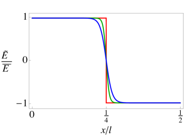
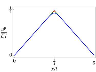
Figure 1: $\tilde{E}/\bar{E}$ (left) and $u^{\smash{\mathrm{p}}}/\bar{E}l$ (right) from (7) on the left half $[0,l/2]$ of the unit cell $[0,l]$ for sharp (red: $\epsilon/l=0$) and smooth (green: $\epsilon/l=1/100$; blue: $\epsilon/l=1/50$) MI interfaces. These and all 1D results to follow are based on $c_{\mathrm{l}}=l/4$, $c_{\mathrm{r}}=3l/4$, and $s_{\mathrm{IM}}=-99/100$ (i.e., $C_{\mathrm{I}}/C_{\mathrm{M}}=S_{\!\mathrm{M}\,}/S_{\!\mathrm{I}\,}=100$). See text for details.

As expected from (3), $\tilde{S}$ determines a continuous and smooth $\tilde{E}$ for $\epsilon>0$, and a discontinuous $\tilde{E}$ for $\epsilon=0$. Likewise, $u^{\smash{\mathrm{p}}}$ is continuous and smooth for $\epsilon>0$, but only continuous for $\epsilon=0$.

2.2 Approximation based on truncated Fourier series

As a first step toward Fourier-series-based numerical solution of the above BVP, consider next the truncated Fourier series approximation of $\tilde{E}$ and $u^{\smash{\mathrm{p}}}$ from (7). The truncated Fourier series of any $f\in L^{2}(0,l)$ is given by

$$\mathcal{F}_{\!\!m\,}f(x):=\sum\nolimits_{\kappa=-m}^{m}e^{\imath k_{\kappa}x}\hat{f}_{\kappa}\,,\quad\hat{f}_{\kappa}:=\frac{1}{l}\int_{0}^{\,l}e^{-\imath k_{\kappa}x}f(x)\ dx\,,$$ (8)

(e.g., Trefethen, 2000; Kopriva, 2009; Liu, 2011) with $\imath:=\sqrt{-1}$ and $k_{\kappa}:=2\pi\kappa/l$. As is well-known, $\mathcal{F}_{\!\!\infty\,}f(x)\neq f(x)$ in general at one or more $x\in[0,l]$. In particular, for $f$ discontinuous on $[0,l]$, then, $\mathcal{F}_{\!\!m\,}f$ deviates from $f$ due to (i) $\mathcal{F}_{\!\!\infty\,}f(x)\neq f(x)$ at points of discontinuity $x\in[0,l]$, and (ii) truncation of $\mathcal{F}_{\!\!\infty\,}f$. Since (i) is related to the Gibbs phenomenon, it will be referred to as Gibbs error in what follows. In the sharp ($\epsilon=0$) MI interface case, then, $\mathcal{F}_{\!\!m\,}\tilde{E}$ is affected by (i) and (ii), whereas $\mathcal{F}_{\!\!m\,}u^{\smash{\mathrm{p}}}$ is affected only by (ii). These are displayed in Figure 2.

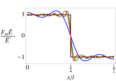
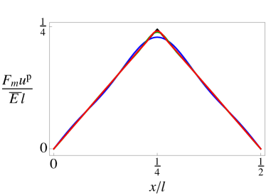
Figure 2: Normalized Fourier series approximation $\mathcal{F}_{\!\!m\,}\tilde{E}(x)/\bar{E}$ (left) and $\mathcal{F}_{\!\!m\,}u^{\smash{\mathrm{p}}}(x)/\bar{E}l$ (right) of $\tilde{E}(x)$ and $u^{\smash{\mathrm{p}}}(x)$, respectively, on the left half unit cell $[0,l/2]$ for discontinuous ($\epsilon=0$) compliance and different degrees of truncation $m<\infty$. In particular, $m=5$ (blue), $m=15$ (green), and $m=25$ (red). The corresponding normalized analytic relations $\tilde{E}(x)/\bar{E}$ and $u^{\smash{\mathrm{p}}}(x)/\bar{E}l$ from (7) are shown (black) for comparison.

As expected, $\lim_{m\to\infty}\mathcal{F}_{\!\!m\,}\tilde{E}(x)\neq\tilde{E}(x)$ at $x=l/4$; rather, $\lim_{m\to\infty}\mathcal{F}_{\!\!m\,}\tilde{E}(l/4)=\frac{1}{2}\lim_{x\,\uparrow\,l/4}\tilde{E}(x)+\frac{1}{2}\lim_{x\,\downarrow\,l/4}\tilde{E}(x)$. Being due to approximation of discontinuous $\tilde{E}$ by $\mathcal{F}_{\!\!\infty\,}\tilde{E}$, note that Gibbs error is unaffected by truncation of $\mathcal{F}_{\!\!\infty\,}\tilde{E}$ to $\mathcal{F}_{\!\!m\,}\tilde{E}$, i.e., independent of $m$. In addition, it is independent of the magnitude of $S_{\!\mathrm{IM}}$.

3 Numerical solution algorithms in 1D

3.1 Algorithms based on trapezoidal discretization

As discussed in the introduction, algorithms for the numerical solution of the current BVP are based on (i) discretization of (8) in 1D, and (ii) tensor-product generalization of these to 3D. More specifically, two discretizations of (8) are considered and compared in this work. The most common of these is trapezoidal discretization of (8)₂ based on that $[0,l]=\bigcup_{i=1}^{n}[x_{i},x_{i+1}]$ of $[0,l]$ with nodes at $x_{i}=(i-1)h$ and nodal spacing $h=l/n$. In this case, (8)₂ and $\hat{f}_{\smash{\kappa}}$ discretizes to

$$\hat{f}_{\smash{\kappa}}^{\mathrm{t}}:=n^{-1/2}\check{f}_{\kappa}^{\mathrm{t}}\,,\quad\check{f}_{\kappa}^{\mathrm{t}}:=n^{-1/2}\sum\nolimits_{i=1}^{n}e^{-\imath k_{\kappa}x_{i}}f_{i}^{\mathrm{t}}\,,$$ (9)

("t" stands for "trapezoidal"). As detailed in Appendix A, (9) induces the trapezoidal discretization (TD)

$$f_{\mathrm{T}}(x):=\varphi_{\mu}^{\mathrm{t}}(x)\,\check{f}_{\mu}^{\mathrm{t}}\,,\quad\varphi_{\mu}^{\mathrm{t}}(x):=n^{-1/2}e^{q_{\mu}x}\,,\quad f_{i}^{\mathrm{t}}=F_{\!\smash{\mu i}\,}^{\mathrm{t}+}\check{f}_{\mu}^{\mathrm{t}}\,,\quad\check{f}_{\mu}^{\mathrm{t}}=F_{\!\smash{\mu i}\,}^{\mathrm{t}-}f_{i}^{\mathrm{t}}\,,$$ (10)

of (8) via (A.6) for $i,\mu=1,\ldots,n$. Here, $\check{f}_{\smash{\mu}}^{\mathrm{t}}\equiv\check{f}_{\smash{\kappa=\mu-1-m}}^{\mathrm{t}}$, $q_{\mu}:=\imath k_{\mu-1-m}$, $f_{\smash{i}}^{\mathrm{t}}\equiv f(x_{i})$, and $F_{\!\smash{\mu i}}^{\mathrm{t}\pm}:=n^{-1/2}e^{\pm q_{\mu}x_{i}}$ from (A.7). If $\bar{f}$ is prescribed, note that $\check{f}_{\smash{\mu=m+1}}^{\mathrm{t}}=\check{f}_{\smash{\kappa=0}}^{\mathrm{t}}=n^{-1/2}\sum_{i=1}^{n}f_{\smash{i}}^{\mathrm{t}}=n^{1/2}\bar{f}$ is determined for a given discretization. For notational simplicity, the "$\mathrm{t}$" superscript for "trapezoidal" is dropped in what follows.

As discussed in the introduction, following previous work (e.g., Dreyer and Müller, 2000; Moulinec and Silva, 2014; Willot, 2015), finite difference discretization (FDD) of differential operators in the context of (10) is employed here for improved robustness in convergence. For example,

$$u_{\smash{\mathrm{T}}}^{\mathrm{p}}(x)=\varphi_{\mu}(x)\,\check{u}_{\mu}^{\smash{\mathrm{p}}}\,,\quad\nabla^{a}u_{\mathrm{T}}^{\smash{\mathrm{p}}}(x)=\varphi_{\mu}(x)\,\check{u}_{\mu}^{\smash{\mathrm{p}}}\otimes q_{\mu}^{a}\,,$$ (11)

via FDD of $\nabla$ in terms of the effective wavenumber $q_{\smash{\mu}}^{a}$. In particular,

$$\begin{array}[]{rclclcl}\nabla^{\mathrm{FD}}u_{\mathrm{T}}^{\smash{\mathrm{p}}}(x)&:=&h^{-1}[u_{\mathrm{T}}^{\smash{\mathrm{p}}}(x+h)-u_{\mathrm{T}}^{\smash{\mathrm{p}}}(x)]&=&\varphi_{\mu}(x)\,{\check{u\mkern 2.0mu}\mkern-2.0mu}{}_{\mu}^{\smash{\mathrm{p}}}\otimes q_{\mu}^{\mathrm{FD}}&=:&\tilde{E}_{\mathrm{FD}}(x)\,,\\ \nabla^{\mathrm{BD}}u_{\mathrm{T}}^{\smash{\mathrm{p}}}(x)&:=&h^{-1}[u_{\mathrm{T}}^{\smash{\mathrm{p}}}(x)-u_{\mathrm{T}}^{\smash{\mathrm{p}}}(x-h)]&=&\varphi_{\mu}(x)\,{\check{u\mkern 2.0mu}\mkern-2.0mu}{}_{\mu}^{\smash{\mathrm{p}}}\otimes q_{\mu}^{\mathrm{BD}}&=:&\tilde{E}_{\mathrm{BD}}(x)\,,\\ \nabla^{\mathrm{CD}}u_{\mathrm{T}}^{\smash{\mathrm{p}}}(x)&:=&\frac{1}{2}h^{-1}[u_{\mathrm{T}}^{\smash{\mathrm{p}}}(x+h)-u_{\mathrm{T}}^{\smash{\mathrm{p}}}(x-h)]&=&\varphi_{\mu}(x)\,{\check{u\mkern 2.0mu}\mkern-2.0mu}{}_{\mu}^{\smash{\mathrm{p}}}\otimes q_{\mu}^{\mathrm{CD}}&=:&\tilde{E}_{\mathrm{CD}}(x)\,,\\ \nabla^{\mathrm{hC}}u_{\mathrm{T}}^{\smash{\mathrm{p}}}(x)&:=&h^{-1}[u_{\mathrm{T}}^{\smash{\mathrm{p}}}(x+\tfrac{1}{2}h)-u_{\mathrm{T}}^{\smash{\mathrm{p}}}(x-\tfrac{1}{2}h))]&=&\varphi_{\mu}(x)\,{\check{u\mkern 2.0mu}\mkern-2.0mu}{}_{\mu}^{\smash{\mathrm{p}}}\otimes q_{\mu}^{\mathrm{hC}}&=:&\tilde{E}_{\mathrm{hC}}(x)\,,\end{array}$$ (12)

for forward ($a=\mathrm{FD}$), backward ($a=\mathrm{BD}$), central ($a=\mathrm{CD}$), and half central ($a=\mathrm{hC}$), difference discretization, respectively, with

$$q_{\mu}^{\mathrm{FD}}:=h^{-1}(e^{q_{\mu}h}-1)\,,\quad q_{\mu}^{\mathrm{BD}}:=h^{-1}(1-e^{-q_{\mu}h})\,,$$ (13)

and

$$q_{\mu}^{\mathrm{CD}}:=h^{-1}\sinh(q_{\mu}h)\,,\quad q_{\mu}^{\mathrm{hC}}:=2h^{-1}\sinh(\tfrac{1}{2}q_{\mu}h)\,.$$ (14)

Analogous to (11), TD of $T(x)$ yields

$$T_{\!\mathrm{T}\,}(x)=\varphi_{\mu}(x)\ \check{T}_{\!\mu\,}\,,\quad\mathrm{div}^{b}T_{\!\mathrm{T}\,}(x)=\varphi_{\mu}(x)\ \check{T}_{\!\mu\,}q_{\mu}^{b}\,,$$ (15)

via FDD of the divergence operator. Together, (11)₂ and (15)₂ induce the preconditioned form

$$-\mathrm{div}^{b}C_{\!\mathrm{H}}[\nabla^{a}u_{\mathrm{T}}^{\smash{\mathrm{p}}}(x)]=\varphi_{\mu}(x)\ \check{G}_{\mathrm{H}}^{-1}(q_{\mu}^{a},q_{\mu}^{b})\,{\check{u\mkern 2.0mu}\mkern-2.0mu}{}_{\mu}^{\smash{\mathrm{p}}}$$ (16)

of the homogenous elliptic operator with

$$\check{G}_{\mathrm{H}}^{-1}(q_{\mu}^{a},q_{\mu}^{b})\,{\check{u\mkern 2.0mu}\mkern-2.0mu}{}_{\mu}^{\smash{\mathrm{p}}}:=-C_{\mathrm{H}}[{\check{u\mkern 2.0mu}\mkern-2.0mu}{}_{\mu}^{\smash{\mathrm{p}}}\otimes q_{\mu}^{a}]\,q_{\mu}^{b}\,,\quad\check{G}_{\mathrm{H}}(q_{\mu}^{a},q_{\mu}^{b})=-1/(C_{\mathrm{H}}\,q_{\mu}^{a}\,q_{\mu}^{b})\,,$$ (17)

the corresponding Green function ($q_{\mu}^{a}\neq 0,q_{\mu}^{b}\neq 0$).

In what follows, $q_{\mu}^{b}$ is determined from a given choice of $a$ in two different ways. The first is based on conjugacy, i.e.,

$$q_{\mu}^{b}=q_{\mu}^{a\ast}$$ (18)

(e.g., Willot, 2015, Equations (19) and (24)). For example, $q_{\mu}^{b}=-q_{\smash{\mu}}^{\mathrm{BD}}$ for $a=\mathrm{FD}$ from (13), or $q_{\mu}^{b}=-q_{\smash{\mu}}^{a}$ for $a=\mathrm{F},\mathrm{CD},\mathrm{hC}$ via (14). The second way is based on the choice $a=\mathrm{FD}$ and the observation that $E_{\mathrm{FD}}(x)=\nabla^{\mathrm{FD}}u(x)$ determines $T(x+\tfrac{1}{2}h)$ via the mean-value theorem. The choice $\mathrm{div}^{\mathrm{BD}}T(x+\tfrac{1}{2}h)$ and identity

$$\nabla^{\mathrm{BD}}\!f(x+\tfrac{1}{2}h)=\nabla^{\mathrm{hC}}\!f(x)$$ (19)

then result in the combination $(a,b)=(\mathrm{FD},\mathrm{hC})$. For this choice, then, both the stress divergence and displacement are calculated at $x$. Note that this choice does not satisfy (18).

The above results are incorporated in Algorithm TD1.

1. given: $n$, $C(x)$, $\bar{E}$, $C_{\mathrm{H}}$, $\check{G}_{\mathrm{H}\,\mu}^{ab}:=\check{G}_{\mathrm{H}}(q_{\smash{\mu}}^{a},q_{\smash{\mu}}^{b})$

2. initialization $\iota=0$

   • for $i=1,\ldots,n$
     ${}\ C_{i}=C(x_{i})$; ${}\ T_{\!\smash{i}}^{(\iota)}=C_{i}\bar{E}$;

   • for $\mu=1,\ldots,n$
     ${}\ {\check{u\mkern 2.0mu}\mkern-2.0mu}{}_{\smash{\mu}}^{\mathrm{p}(\iota)}=0$; ${}\ \check{T}_{\!\smash{\mu}}^{(\iota)}=F_{\!\smash{\mu i}\,}^{-}T_{\!\smash{i}}^{(\iota)}$; ${}\ \Delta{\check{u\mkern 2.0mu}\mkern-2.0mu}{}_{\smash{\mu}}^{\mathrm{p}(\iota)}=\check{G}_{\smash{\mathrm{H}\,\mu}}^{ab}\check{T}_{\!\smash{\mu}}^{(\iota)}q_{\smash{\mu}}^{b}$;

   • $\iota\!+\!\!+$;

3. while $\sum_{\mu=1}^{n}|\Delta{\check{u\mkern 2.0mu}\mkern-2.0mu}{}_{\smash{\mu}}^{\mathrm{p}(\iota)}-\Delta{\check{u\mkern 2.0mu}\mkern-2.0mu}{}_{\smash{\mu}}^{\mathrm{p}(\iota-1)}|\geqslant\mathrm{tol}$ & $\iota\leqslant\mathrm{maxit}$

   • for $i=1,\ldots,n$
     ${}\ \tilde{E}_{\smash{i}}^{(\iota)}=F_{\!\smash{\mu i}\,}^{+}{\check{u\mkern 2.0mu}\mkern-2.0mu}{}_{\smash{\mu}}^{\mathrm{p}(\iota)}\otimes q_{\mu}^{a}$; ${}\ T_{\!\smash{i}}^{(\iota)}=T_{\!\smash{i}}^{(0)}+C_{i}\tilde{E}_{\smash{i}}^{(\iota)};$

   • for $\mu=1,\ldots,n$
     ${}\ \check{T}_{\!\smash{\mu}}^{(\iota)}=F_{\!\smash{\mu i}\,}^{-}T_{\!\smash{i}}^{(\iota)}$; ${}\ \Delta{\check{u\mkern 2.0mu}\mkern-2.0mu}{}_{\smash{\mu}}^{\mathrm{p}(\iota)}=\check{G}_{\smash{\mathrm{H}\,\mu}}^{ab}\check{T}_{\!\smash{\mu}}^{(\iota)}q_{\smash{\mu}}^{b}$; ${}\ {\check{u\mkern 2.0mu}\mkern-2.0mu}{}_{\mu}^{\smash{\mathrm{p}}(\iota)}+\!=\Delta{\check{u\mkern 2.0mu}\mkern-2.0mu}{}_{\mu}^{\smash{\mathrm{p}}(\iota)}$;

   • $\iota\!+\!\!+$;

Algorithm TD1

The direct Fourier case is included here by defining $q_{\smash{\mu}}^{\mathrm{F}}:=q_{\mu}$ ("F" for "Fourier"). Rather than being strain-based like the "basic scheme" of Suquet (1997) and Michel et al. (2000, 2001), note that Algorithm TD1 is displacement-based. As evident from (17), $\check{G}_{\mathrm{H}}^{-1}(q_{\smash{\mu}}^{a},q_{\smash{\mu}}^{b})$ is not invertible when either $q_{\smash{\mu}}^{a}$ or $q_{\smash{\mu}}^{b}$ vanish. For $n$ even, (13) and (14) imply $q_{\smash{\mu}}^{a,b}=0$ at $\mu=m+1$ for $a,b=\mathrm{F},\mathrm{FD},\mathrm{BD},\mathrm{hC}$, and at $\mu=1,m+1$ for $a,b=\mathrm{CD}$. For this latter case, we follow Willot (2015, Equation (29)) and formally set $\check{G}_{\mathrm{H}}(q_{\smash{\mu}}^{a},q_{\smash{\mu}}^{b})\equiv 0$ for $\mu=1$. For $n$ odd, $q_{\smash{\mu}}^{a,b}=0$ only at $\mu=m+1$ for all cases.

3.2 Algorithms based on piecewise-constant discretization

Assume now that $f(x)$ in (8)₂ is constant on each subinterval $[x_{i},x_{i+1}]$ of $[0,l]$ with value $f_{\smash{i}}^{\mathrm{c}}\equiv f(x_{\smash{i}}^{\mathrm{c}})$ at the mid-point or "center" $x_{i}^{\mathrm{c}}=(i-\frac{1}{2})\,h$ of $[x_{i},x_{i+1}]$. In this case, $\hat{f}_{\kappa}$ in (8)₂ reduces to

$$\hat{f}_{\kappa}^{\mathrm{c}}:=n^{-1/2}s_{\kappa}\,\check{f}_{\kappa}^{\mathrm{c}}\,,\quad s_{\kappa}:=\mathop{\mathrm{sinc}}(\pi\kappa/n)\,,\quad\check{f}_{\kappa}^{\mathrm{c}}:=n^{-1/2}\sum\nolimits_{i=1}^{n}e^{-\imath k_{\kappa}x_{i}^{\mathrm{c}}}f_{i}^{\mathrm{c}}\,,$$ (20)

with $\mathop{\mathrm{sinc}}(x):=\sin(x)/x$ the (unnormalized) sinc function. As shown by comparison of $\hat{f}_{\kappa}^{\mathrm{c}}$ with $\hat{f}_{\kappa}^{\mathrm{t}}$ from (9), differences between these include (i) the dependence of $\hat{f}_{\kappa}^{\mathrm{c}}$ on the sinc "filter" $s_{\kappa}$, and (ii) different discretizations of $[0,l]$. Leaving the details to Appendix B, (20) results in the piecewise-constant discretization (PCD)

$$f_{\mathrm{PC}}(x):=\varphi_{\mu}^{\mathrm{c}}(x)\,\check{f}_{\mu}^{\mathrm{c}}\,,\quad\varphi_{\mu}^{\mathrm{c}}(x):=s_{\mu}^{\mathrm{c}}\,\varphi_{\mu}^{\mathrm{t}}(x)\,,\quad f_{i}^{\mathrm{c}}=F_{\!\smash{\mu i}\,}^{\mathrm{c}+}\check{f}_{\mu}^{\mathrm{c}}\,,\quad\check{f}_{\mu}^{\mathrm{c}}=F_{\!\smash{\mu i}\,}^{\mathrm{c}-}f_{i}^{\mathrm{c}}\,,$$ (21)

of (8) via (B.8) for $i,\mu=1,\ldots,n$, analogous to (10) in the TD case, with $s_{\smash{\mu}}^{\mathrm{c}}:=s_{\mu-1-m}$ and $F_{\!\smash{\mu i}\,}^{\mathrm{c}\pm}:=n^{-1/2}e^{\pm q_{\mu}x_{i}^{\mathrm{c}}}$. In particular, $s_{\smash{m+1}}^{\mathrm{c}}=s_{0}=1$ and $\check{f}_{\smash{\mu=m+1}}^{\mathrm{c}}=\check{f}_{\smash{\kappa=0}}^{\mathrm{c}}=n^{-1/2}\sum_{i=1}^{n}f_{i}^{\mathrm{c}}=n^{1/2}\bar{f}$. Analogous to (11) and (15), then, we have

$$u_{\mathrm{PC}}^{\smash{\mathrm{p}}}(x)=\varphi_{\smash{\mu}}^{\mathrm{c}}(x)\ \check{u}_{\smash{\mu}}^{\mathrm{pc}}\,,\quad T_{\!\mathrm{PC}}(x)=\varphi_{\smash{\mu}}^{\mathrm{c}}(x)\ \check{T}_{\!\smash{\mu}}^{\mathrm{c}}\,,$$ (22)

and

$$\nabla^{a}\!u_{\mathrm{PC}}^{\mathrm{p}}(x)=\varphi_{\mu}^{\mathrm{c}}(x)\ \check{u}_{\mu}^{\mathrm{pc}}\otimes q_{\mu}^{a}\,,\ \ \mathrm{div}^{b}T_{\mathrm{PC}}^{\mathrm{c}}(x)=\varphi_{\mu}^{\mathrm{c}}(x)\,\check{T}_{\!\mu}^{\mathrm{c}}\,q_{\mu}^{b}\,.$$ (23)

Further,

$$-\mathrm{div}^{b}C_{\!\mathrm{H}}[\nabla^{a}\!u_{\mathrm{PC}}^{\smash{\mathrm{p}}}(x)]=\varphi_{\mu}^{\mathrm{c}}(x)\ \check{G}_{\mathrm{H}}^{-1}(q_{\mu}^{a},q_{\mu}^{b})\,\check{u}_{\mu}^{\mathrm{pc}}\,,$$ (24)

analogous to (16). Completely analogous to the case of Algorithm TD1, then, these relations and the fact that $s_{\smash{\mu}}^{\mathrm{c}}\neq 0$ can be employed to obtain Algorithm PCD1.

1. given: $n$, $C(x)$, $\bar{E}$, $C_{\mathrm{H}}$, $\check{G}_{\mathrm{H}\,\mu}^{ab}:=\check{G}_{\mathrm{H}}(q_{\smash{\mu}}^{a},q_{\smash{\mu}}^{b})$

2. initialization $\iota=0$

   • for $i=1,\ldots,n$
     ${}\ C_{\smash{i}}^{\mathrm{c}}=C(x_{\smash{i}}^{\mathrm{c}})$; ${}\ T_{\!\smash{i}}^{\mathrm{c}(\iota)}=C_{\smash{i}}^{\mathrm{c}}\bar{E}$;

   • for $\mu=1,\ldots,n$
     ${}\ \ {\check{u\mkern 2.0mu}\mkern-2.0mu}{}_{\mu}^{\smash{\mathrm{pc}(\iota)}}=0$; ${}\ \check{T}_{\!\smash{\mu}}^{\mathrm{c}(\iota)}=F_{\!\smash{\mu i}\,}^{-}T_{\!\smash{i}}^{\mathrm{c}(\iota)}$; ${}\ \Delta{\check{u\mkern 2.0mu}\mkern-2.0mu}{}_{\smash{\mu}}^{\mathrm{pc}(\iota)}=\check{G}_{\smash{\mathrm{H}\,\mu}}^{ab}\check{T}_{\!\smash{\mu}}^{\mathrm{c}(\iota)}q_{\smash{\mu}}^{b}$;

   • $\iota\!+\!\!+$;

3. while $\sum_{\mu=1}^{n}|\Delta{\check{u\mkern 2.0mu}\mkern-2.0mu}{}_{\smash{\mu}}^{\mathrm{pc}(\iota)}-\Delta{\check{u\mkern 2.0mu}\mkern-2.0mu}{}_{\smash{\mu}}^{\mathrm{pc}(\iota-1)}|\geqslant\mathrm{tol}$ & $\iota\leqslant\mathrm{maxit}$

   • for $i=1,\ldots,n$
     ${}\ \tilde{E}_{\smash{i}}^{\mathrm{c}(\iota)}=F_{\!\smash{\mu i}\,}^{\mathrm{c}+}{\check{u\mkern 2.0mu}\mkern-2.0mu}{}_{\smash{\mu}}^{\smash{\mathrm{pc}(\iota)}}\otimes q_{\smash{\mu}}^{a}$; ${}\ T_{\!\smash{i}}^{\mathrm{c}(\iota)}=T_{\!\smash{i}}^{\mathrm{c}(0)}+C_{\smash{i}}^{\mathrm{c}}\tilde{E}_{\smash{i}}^{\mathrm{c}(\iota)};$

   • for $\mu=1,\ldots,n$
     ${}\ \check{T}_{\!\smash{\mu}\,}^{\mathrm{c}(\iota)}=F_{\!\smash{\mu i}\,}^{\mathrm{c}-}T_{\!\smash{i}}^{\mathrm{c}(\iota)}$; ${}\ \Delta{\check{u\mkern 2.0mu}\mkern-2.0mu}{}_{\smash{\mu}}^{\smash{\mathrm{pc}}(\iota)}={\check{G\mkern 4.0mu}\mkern-4.0mu}{}_{\smash{\mathrm{H}\,\mu}}^{ab}\check{T}_{\!\smash{\mu}}^{\mathrm{c}(\iota)}q_{\smash{\mu}}^{b}$; ${}\ {\check{u\mkern 2.0mu}\mkern-2.0mu}{}_{\smash{\mu}}^{\smash{\mathrm{pc}}(\iota)}+\!=\Delta{\check{u\mkern 2.0mu}\mkern-2.0mu}{}_{\smash{\mu}}^{\smash{\mathrm{pc}}(\iota)}$;

   • $\iota\!+\!\!+$;

Algorithm PCD1

As evident, this algorithm is independent of $s_{\smash{\mu}}^{\mathrm{c}}=s_{\mu-1-m}=\mathop{\mathrm{sinc}}(\pi(\mu-1-m)/n)$ from (20)₂. This is in contrast to the PCD-based algorithm of Eloh et al. (2019), to which we now turn.

3.3 Algorithm of Eloh et al. (2019)

Following Brisard and Dormieux (2010), Eloh et al. (2019) recently developed an algorithm also based on PCD and (20) quite different than Algorithm PCD1. To this end, they formulate their algorithm based on $\mathcal{F}_{\!\!\infty\,}^{\mathrm{c}}f(x):=\sum\nolimits_{\kappa=-\infty}^{\infty}e^{\imath k_{\kappa}x}\hat{f}_{\smash{\kappa}}^{\mathrm{c}}$ from (8) for $m=\infty$ and (20), and truncate the result. Equivalently, as done here, one can work with the truncated form

$$\mathcal{F}_{\!\!p\,}^{\mathrm{c}}f(x):=\sum\nolimits_{\kappa=-p}^{p-1}e^{\imath k_{\kappa}x}\hat{f}_{\kappa}^{\mathrm{c}}=n^{-1/2}\sum\nolimits_{\omega=0}^{n-1}e^{\imath k_{\omega}x}\sum\nolimits_{\nu=-m}^{m-1}e^{\imath k_{\nu n}x}s_{\nu n+\omega}\,\check{f}_{\nu n+\omega}^{\mathrm{c}}$$ (25)

of $\mathcal{F}_{\!\!\infty\,}^{\mathrm{c}}f(x)$ from the start (for $p=nm$ even). Combining this with (the second of)

$$\check{f}_{\nu n+\omega}^{\mathrm{c}}=(-1)^{\nu}\check{f}_{\omega}^{\mathrm{c}}\,,\quad n^{-1/2}\sum\nolimits_{\omega=0}^{n-1}e^{\imath k_{\omega}x_{i}^{\mathrm{c}}}\check{f}_{\omega}^{\mathrm{c}}=f(x_{i}^{\mathrm{c}})=f_{i}^{\mathrm{c}}\,,$$ (26)

from (20)₃ results in the PCD

$$f_{\mathrm{El}}(x):=\varphi_{\omega}^{\mathrm{El}}(x)\,\check{f}_{\omega}^{\mathrm{c}}\,,\quad\varphi_{\omega}^{\mathrm{El}}(x):=n^{-1/2}\sum\nolimits_{\nu=-m}^{m-1}e^{\imath k_{\nu n+\omega}x}\,(-1)^{\nu}s_{\nu n+\omega}\,,$$ (27)

(sum over repeated $\omega$) of (8) for $\omega=0,\ldots,n-1$, analogous to (21) ("El" stands for "Eloh"). As in the basic scheme (e.g., Suquet, 1997), they work with (i) strain $\tilde{E}_{\mathrm{El}}(x)=\varphi_{\omega}^{\mathrm{El}}(x)\,\check{\tilde{E}}_{\omega}^{\mathrm{c}}$ as the primary discretant, and (ii) the Fourier transform

$${\hat{\Gamma\mkern 4.0mu}\mkern-4.0mu}{}_{\!\!\mathrm{H}}(k)\,\hat{T}(k)=-{\hat{G\mkern 4.0mu}\mkern-4.0mu}{}_{\mathrm{H}}(k)\,\hat{T}(k)\,k\otimes k=0\,,\quad k\neq 0\,,$$ (28)

of mechanical equilbrium $\Gamma_{\!\!\mathrm{H}}\ast T:=\nabla G_{\mathrm{H}}\ast\mathop{\mathrm{div}}T=0$ in pre-conditioned Lippmann-Schwinger form. Again leaving the details to Appendix B, this results in Algorithm DGO1.

1. given: $n$, $m$, $C(x)$, $\bar{E}$, $C_{\mathrm{H}}$, ${\check{\Gamma\mkern 4.0mu}\mkern-4.0mu}{}_{\!\!\smash{\mathrm{H}\,\omega=0}}^{\mathrm{c}}=0$, ${\check{\Gamma\mkern 4.0mu}\mkern-4.0mu}{}_{\!\!\smash{\mathrm{H}\,\omega\neq 0}}^{\mathrm{c}}=\sum\nolimits_{\nu=-m}^{m-1}s_{\nu n+\omega}\ {\hat{\Gamma\mkern 4.0mu}\mkern-4.0mu}{}_{\!\!\mathrm{H}}(k_{\nu n+\omega})$

2. initialization $\iota=0$

   • for $i=1,\ldots,n$
     ${}\ C_{\smash{i}}^{\mathrm{c}}=C(x_{\smash{i}}^{\mathrm{c}})$; ${}\ T_{\!\smash{i}}^{\mathrm{c}(\iota)}=C_{\smash{i}}^{\mathrm{c}}\bar{E}$;

   • for $\omega=0,\ldots,n-1$
     ${}\ \check{E}_{\smash{\omega}}^{\mathrm{c}(\iota)}=0$; ${}\ \check{T}_{\!\smash{\omega}}^{\mathrm{c}(\iota)}=F_{\!\smash{\omega i}\,}^{-}T_{\!\smash{i}}^{\mathrm{c}(\iota)}$; ${}\ \Delta\check{E}_{\smash{\omega}}^{\mathrm{c}(\iota)}={\check{\Gamma\mkern 4.0mu}\mkern-4.0mu}{}_{\!\!\smash{\mathrm{H}\,\omega}\,}^{\mathrm{c}}{\check{T\mkern 4.0mu}\mkern-4.0mu}{}_{\!\smash{\omega}}^{\mathrm{c}(\iota)}$;

   • $\iota\!+\!\!+$;

3. while $\sum_{\omega=1}^{n-1}|\Delta\check{E}_{\omega}^{\mathrm{c}(\iota)}-\Delta\check{E}_{\omega}^{\mathrm{c}(\iota-1)}|\geqslant\mathrm{tol}$ & $\iota\leqslant\mathrm{maxit}$

   • for $i=1,\ldots,n$
     ${}\ \tilde{E}_{\smash{i}}^{\mathrm{c}(\iota)}=\check{F}_{\smash{\omega i}}^{\mathrm{c}+}\check{E}_{\smash{\omega}}^{\mathrm{c}(\iota)}$; ${}\ T_{\!\smash{i}}^{\mathrm{c}(\iota)}=T_{\!\smash{i}}^{\mathrm{c}(0)}+C_{\smash{i}}^{\mathrm{c}}\tilde{E}_{\smash{i}}^{\mathrm{c}(\iota)}$;

   • for $\omega=0,\ldots,n-1$
     ${}\ {\check{T\mkern 4.0mu}\mkern-4.0mu}{}_{\!\smash{\omega}}^{\mathrm{c}(\iota)}=\check{F}_{\!\smash{\omega i}\,}^{\mathrm{c}-}T_{\!\smash{i}}^{\mathrm{c}(\iota)}$; ${}\ \Delta\check{E}_{\smash{\omega}}^{\mathrm{c}(\iota)}={\check{\Gamma\mkern 4.0mu}\mkern-4.0mu}{}_{\!\!\smash{\mathrm{H}\omega}\,}^{\mathrm{c}}{\check{T\mkern 4.0mu}\mkern-4.0mu}{}_{\!\smash{\omega}}^{\mathrm{c}(\iota)}$; ${}\ \check{E}_{\smash{\omega}}^{\mathrm{c}(\iota)}+\!=\Delta\check{E}_{\smash{\omega}}^{\mathrm{c}(\iota)}$;

   • $\iota\!+\!\!+$;

Algorithm DGO1

Here, $\check{F}_{\!\smash{\omega i}}^{\mathrm{c}\pm}:=n^{-1/2}e^{\pm\imath k_{\omega}x_{\smash{i}}^{\mathrm{c}}}$ and $k_{\nu n+\omega}=2\pi(\nu n+\omega)/l=2\pi(\nu+\omega/n)/h$. Again, a sum on repeated $i$, $\omega$ is employed. Note the dependence of the discretized Lippmann-Schwinger operator ${\check{\Gamma\mkern 4.0mu}\mkern-4.0mu}{}_{\!\!\smash{\mathrm{H}\,\omega}}^{\mathrm{c}}$ on $s_{-mn+\omega}$, $\ldots$, $s_{(m-1)n+\omega}$. As already noted above, this is one difference between the two PCD-based algorithms PCD1 and DGO1.

4 Computational comparisons in 1D

Employing the algorithms just discussed, the 1D BVP for the periodic MI case is now solved numerically and compared with the analytical solution. To this end, the unit cell from the analytic case in Section 2 as based on $C_{\mathrm{I}}/C_{\mathrm{M}}=100$ is employed, and the homogeneous stiffness $C_{\mathrm{H}}$ is determined by $C_{\mathrm{H}}=\frac{1}{2}(C_{\mathrm{M}}+C_{\mathrm{I}})$.

Since $C(x)$ is not defined on the MI interface in the discontinuous case, note that this interface always lies between two nodes, one in the matrix, and the other in the inclusion. This is in contrast to the smooth case, for which $C(x)$ is defined everywhere. The stiffness profile $C(x)=1/S\!(x)$ for the smooth interface is based on $\nu(x)$ with $\epsilon/l=1/100$. To be comparible with the analytic results in Figure 1, the following numerical results are based on deformation control and $\bar{E}=1$. In the context of (18), results are obtained and compared for $a=\mathrm{F},\mathrm{CD},\mathrm{FD}$. These are obtained as well for $(a,b)=(\mathrm{FD},\mathrm{hC})$. In all cases, the tolerance $\mathrm{tol}$ is machine precision.

To begin, consider the results for $\tilde{E}(x)$ in Figure 3.

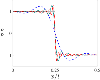
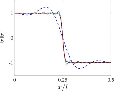
Figure 3: Comparison of results for $\tilde{E}_{a}(x)=\varphi_{\mu}(x)\,\check{u}_{\mu}^{\smash{\mathrm{p}}}\otimes q_{\mu}^{a}$ obtained from Algorithm TD1 with the analytic result $\tilde{E}(x)$ (black curve) from (7)₁ across a sharp (left) and a smooth (right) MI interface at $x/l=1/4$ for the discretizations (i) $n=10$ ($m=5$; blue curve), (ii) $n=50$ ($m=25$; green curve), (iii) $n=90$ ($m=45$; red curve). As done in Figures 1 and 2 above, results are shown here and in what follows for the left half of the unit cell.

As implied by these results, all choices considered for $q_{\mu}^{a}$ and $q_{\mu}^{b}$ in the context of Algorithm TD1 yield the same solution for $\tilde{E}_{a}(x)$ at both sharp (Figure 3, left) and smooth (Figure 3, right) MI interfaces. Moreover, as expected from Fourier series approximation of the analytic solution and series truncation (Figure 2, left), $\tilde{E}_{a}(x)$ at the sharp MI interface (left) exhibits Gibbs error whose magnitude is independent of numerical resolution. This is in contrast to $\tilde{E}_{a}(x)$ at the smooth MI interface (Figure 3, right), which does converge in this fashion, again as expected.

Consider next the comparison of results from Algorithms TD1 and PCD1 for the case of a sharp MI interface shown in Figure 4

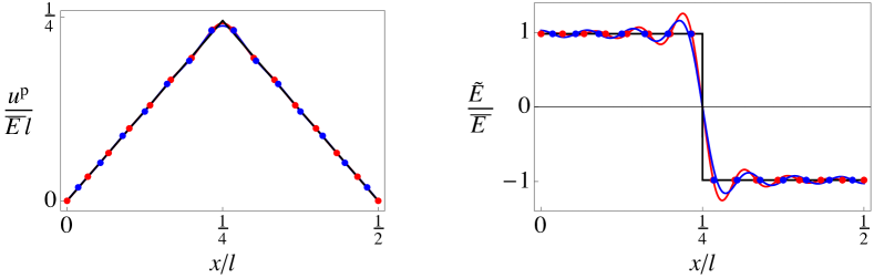
Figure 4: Left: comparison of results for $u_{\smash{\mathrm{T}}}^{\mathrm{p}}(x)=\varphi_{\mu}(x)\,{\check{u\mkern 2.0mu}\mkern-2.0mu}{}_{\smash{\mu}}^{\mathrm{p}}$ from Algorithm TD1 (red points, curve) and for $u_{\smash{\mathrm{PC}}}^{\mathrm{p}}(x)=\varphi_{\smash{\mu}}^{\mathrm{c}}(x)\,\check{u}_{\smash{\mu}}^{\mathrm{pc}}$ from Algorithm PCD1 (blue points, curve) with analytic solution (black curve) across a sharp MI interface at $x/l=0.25$. Right: comparison of results for $\tilde{E}_{\mathrm{T}}(x):=\nabla^{\smash{\mathrm{F}}}\!u_{\smash{\mathrm{T}}}^{\mathrm{p}}(x)=\varphi_{\mu}(x)\,\check{u}_{\smash{\mu}}^{\smash{\mathrm{p}}}\otimes q_{\smash{\mu}}^{\mathrm{F}}$ from Algorithm TD1 (red points, curve) and for $\tilde{E}_{\mathrm{PC}}(x):=\nabla^{\mathrm{F}}\!u_{\smash{\mathrm{PC}}}^{\mathrm{p}}(x)=\varphi_{\smash{\mu}}^{\mathrm{c}}(x)\,\check{u}_{\smash{\mu}}^{\mathrm{pc}}\otimes q_{\mu}^{\mathrm{F}}$ from Algorithm PCD1 (blue points, curve) with analytic solution (black curve). Results are based on discretizations of $n=30$ ($m=15$; red points) and $n=32$ ($m=16$; blue points).

As seen in particular in the strain results on the right, the dependence of $\varphi_{\mu}^{\mathrm{c}}(x)$ in (21) on $s_{\mu}^{\mathrm{c}}$ dampens Gibbs oscillations / error in $\tilde{E}_{\mathrm{PC}}(x)$ in comparison to $\tilde{E}_{\mathrm{T}}(x)$. As expected, this has no effect on the numerical (i.e., collocation) solution at the nodes, in contrast to the analogous results from Algorithm DGO1 in Figure 5.

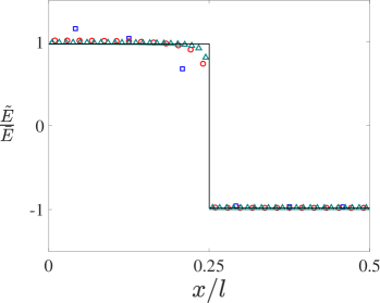
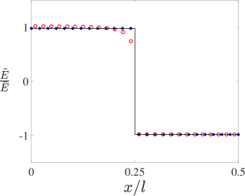
Figure 5: Left: Results for nodal $\tilde{E}_{i}^{\mathrm{c}}$ from Algorithm DGO1 across a sharp MI interface at $x/l=1/4$ for the discretizations (i) $n=10$ ($m=5$; blue squares), (ii) $n=50$ ($m=25$; red circles), (iii) $n=90$ ($m=45$; green triangles), compared with the analytic result $\tilde{E}(x)$ (black curve) from (7)₁. Righ: Comparison of results for nodal $\tilde{E}_{i}$ from Algorithm TD1 (blue asterisks) and those for $\tilde{E}_{i}^{\mathrm{c}}$ from Algorithm DGO1 (red circles) for the discretization $n=50$ ($m=25$).

As shown on the left, the nodal results from Algorithm DGO1 deviate slightly from those of the anayltic solution in the (relatively soft) matrix, with maximum deviation in the matrix next to the MI interface. Note that this deviation decreases with increasing numerical resolution. This is in contrast to the analogous solutions from Algorithm TD1 (and so Algorithm PCD1) as shown by the comparison on the right. One difference between the PCD-based Algorithms PCD1 and DGO1 that is likely playing a role here is the dependence of the discretized Lippmann-Schwinger operator ${\check{\Gamma\mkern 4.0mu}\mkern-4.0mu}{}_{\!\!\smash{\mathrm{H}\,\omega}}^{\mathrm{c}}$ on $s_{\nu n+\omega}$ in Algorithm DGO1. These and other differences in 1D become even more evident in the context of tensor-product-based generalization of the above 1D algorithms to 3D, to which we now turn.

5 Algorithms for strong mechanical equilibrium in 3D

5.1 Basics

Let $\bm{u}$, $\bm{H}=\nabla\bm{u}$, and $\bm{E}=\mathop{\mathrm{sym}}\bm{H}$ represent the 3D displacement, distortion and strain, respectively. In this case, let $f=\bar{f}+\tilde{f}$ now represent the 3D generalization of (1) with respect to the unit cell $U$. Likewise,

$$\bm{u}=\bm{u}^{\smash{\mathrm{h}}}+\bm{u}^{\smash{\mathrm{p}}}\,,\quad\bm{u}^{\smash{\mathrm{h}}}(\bm{x})=\bm{c}+{\bar{\bm{H}\mkern 3.0mu}\mkern-3.0mu}{}\bm{x}\,,\quad\bm{u}^{\smash{\mathrm{p}}}(\bm{x})=\int{\tilde{\bm{H}\mkern 3.0mu}\mkern-3.0mu}{}(\bm{x})\,d\bm{x}\,,\quad\nabla\bm{u}^{\smash{\mathrm{p}}}={\tilde{\bm{H}\mkern 3.0mu}\mkern-3.0mu}{}\,,$$ (29)

is the generalization of (2) to 3D with $\bar{\bm{u}}^{\smash{\mathrm{p}}}=\bm{0}$, and so $\bar{\bm{u}}^{\smash{\mathrm{h}}}=\bm{c}+{\bar{\bm{H}\mkern 3.0mu}\mkern-3.0mu}{}\bar{\bm{x}}=\bar{\bm{u}}$. As in the 1D case, $\bm{c}$, ${\bar{\bm{H}\mkern 3.0mu}\mkern-3.0mu}{}$, and so $\bm{u}^{\smash{\mathrm{h}}}$, are known, and attention is focused on $\bm{u}^{\smash{\mathrm{p}}}$. On this basis, quasi-static mechanical equilibrium and isotropic, linear elastic material behavior continue to apply. Let $\bm{T}=\mathsfbfit{C}\bm{E}$ be the linear elastic stress, and $\mathsfbfit{C}(\bm{x})=\lambda(\bm{x})\,\bm{I}\otimes\bm{I}+\mu(\bm{x})\,(\bm{I}\,\square\,\bm{I}+\bm{I}\,\triangle\,\bm{I})$ the isotropic stiffness. For the case of discontinuous $\mathsfbfit{C}(\bm{x})$, the following hold at the MI interface (with unit normal $\bm{n}$):  (i) no cracking $\bm{u}_{\mathrm{I}}=\bm{u}_{\mathrm{M}}$, (ii) kinematic compatibility $\bm{H}_{\mathrm{I}}=\bm{H}_{\mathrm{M}}+\bm{h}\otimes\bm{n}$, and (iii) mechanical equilibrium $\bm{T}_{\!\mathrm{I}}\bm{n}=\bm{T}_{\!\mathrm{M}}\bm{n}$. Both $\lambda(\bm{x})$ and $\mu(\bm{x})$ are determined by direct tensor-product generalization of analogous 1D relations like (6) based on $\theta$ in the discontinuous, and on $\nu$ in the continuous, case.

5.2 Algorithm based on trapezoidal discretization

Let $r=1,2,3$. As in the 1D case, consider a uniform discretization of $[0,l_{r}]$ based on $n_{r}+1$ nodes $x_{\smash{i_{r}}}=i_{r}h_{r}$ with $i_{r}=0,\ldots,n_{r}$ and spacing $h_{r}$ such that $l_{r}=n_{r}h_{r}$ ($n_{r}$ subintervals). Direct tensor-product-based generalization of (10)₁ to 3D yields

$$f_{\smash{\mathrm{T}}}(\mathbf{x})=\varphi_{\smash{\mu_{1}}}(x_{1})\,\varphi_{\smash{\mu_{2}}}(x_{2})\,\varphi_{\smash{\mu_{3}}}(x_{3})\,\check{f}_{\smash{\mu_{1}\mu_{2}\mu_{3}}}=:\varphi_{\bm{\mu}}(\mathbf{x})\star\check{f}_{\bm{\mu}}$$ (30)

(sum on repeated indices) in terms of Rayleigh product notation with $\mathbf{x}:=(x_{1},x_{2},x_{3})$ and $\mu_{r}=1,\ldots,n_{r}$, $r=1,2,3$. Here,

$$\begin{array}[]{rclclcl}f_{\mathbf{i}}&:=&f_{\smash{i_{1}i_{2}i_{3}}}&=&F_{\!\smash{\mu_{1}i_{1}}\,}^{+}F_{\!\smash{\mu_{2}i_{2}}\,}^{+}F_{\!\smash{\mu_{3}i_{3}}\,}^{+}\,\check{f}_{\smash{\mu_{1}\mu_{2}\mu_{3}}}&=:&F_{\!\bm{\mu}\mathbf{i}\,}^{+}\star\check{f}_{\bm{\mu}}\,,\\ \check{f}_{\bm{\mu}}&:=&\check{f}_{\smash{\mu_{1}\mu_{2}\mu_{3}}}&=&F_{\!\smash{\mu_{1}i_{1}}\,}^{-}F_{\!\smash{\mu_{2}i_{2}}\,}^{-}F_{\!\smash{\mu_{3}i_{3}}\,}^{-}\,f_{\smash{i_{1}i_{2}i_{3}}}&=:&F_{\!\bm{\mu}\mathbf{i}\,}^{-}\star f_{\mathbf{i}}\,,\end{array}$$ (31)

(sum on repeated indices) via (10)_3,4. Given these, generalization of Algorithm TD1 to 3D is based in particular on those

$$\nabla^{\mathbf{a}}\mathbf{u}_{\smash{\mathrm{T}}}^{\mathrm{p}}(\mathbf{x})=\varphi_{\bm{\mu}}(\mathbf{x})\star\check{\mathbf{u}}_{\bm{\mu}}^{\smash{\mathrm{p}}}\otimes\mathbf{q}_{\bm{\mu}}^{\mathbf{a}}\,,\quad\mathrm{div}^{\mathbf{b}}\mathbf{T}_{\mathrm{T}}(\mathbf{x})=\varphi_{\bm{\mu}}(\mathbf{x})\star\,\check{\mathbf{T}}_{\!\bm{\mu}\,}\mathbf{q}_{\bm{\mu}}^{\mathbf{b}}\,,$$ (32)

of (11)₁ and (15)₂, respectively. Here, $\check{\mathbf{u}}_{\smash{\bm{\mu}}}^{\mathrm{p}}:=(\check{u}_{\smash{1\bm{\mu}}}^{\mathrm{p}},\check{u}_{\smash{2\bm{\mu}}}^{\mathrm{p}},\check{u}_{\smash{3\bm{\mu}}}^{\mathrm{p}})$, $\check{\mathbf{T}}_{\!\bm{\mu}\,}$ is the $3\times 3$ symmetric matrix of stress components, and $\mathbf{q}_{\smash{\bm{\mu}}}^{\mathbf{a}}:=(q_{\smash{\mu_{1}}}^{a_{1}},q_{\smash{\mu_{2}}}^{a_{2}},q_{\smash{\mu_{3}}}^{a_{3}})$ with $q_{\smash{\mu_{r}}}:=\imath k_{\smash{\mu_{r}-1-m_{r}}}$. As in the 1D case (17), 3D quasi-static momentum balance is formulated algorithmically in preconditioned form based on the Green function $\check{\mathbf{G}}_{\mathrm{H}}(\mathbf{q}_{\smash{\bm{\mu}}}^{\mathbf{a}},\mathbf{q}_{\smash{\bm{\mu}}}^{\mathbf{b}})$ of the corresponding operator

$$-\mathrm{div}^{\mathbf{b}}\,\textsf{C}_{\mathrm{H}}\nabla_{\!\mathbf{h}}^{\mathbf{a}}\mathbf{u}(\mathbf{x})=-\varphi_{\bm{\mu}}(\mathbf{x})\star\textsf{C}_{\mathrm{H}}[\check{\mathbf{u}}_{\bm{\mu}}\otimes\mathbf{q}_{\bm{\mu}}^{\mathbf{a}}]\mathbf{q}_{\bm{\mu}}^{\mathbf{b}}=\varphi_{\bm{\mu}}(\mathbf{x})\star\check{\mathbf{G}}_{\mathrm{H}}^{-1}(\mathbf{q}_{\bm{\mu}}^{\mathbf{a}},\mathbf{q}_{\bm{\mu}}^{\mathbf{b}})\,\check{\mathbf{u}}_{\bm{\mu}}\,.$$ (33)

Given these relations, direct componentwise generalization of Algorithm TD1 yields Algorithm TD2.

1. given: $n_{1},\ldots,n_{3}$, $\mathsfbfit{C}(\bm{x})$, $\bar{\bm{E}}$, $\mathsfbfit{C}_{\mathrm{H}}$, $\check{\mathbf{G}}_{\smash{\mathrm{H}\bm{\mu}}}^{\mathbf{ab}}=\hat{\mathbf{G}}_{\mathrm{H}}(\mathbf{q}_{\smash{\bm{\mu}}}^{\mathbf{a}},\mathbf{q}_{\smash{\bm{\mu}}}^{\mathbf{b}})$

2. initialization $\iota=0$

   • for $i_{1}=1,\ldots,n_{1}$, $\ldots$, $i_{3}=1,\ldots,n_{3}$
     ${}\ \textsf{C}_{\mathbf{i}}=\textsf{C}(\mathbf{x}_{\mathbf{i}})$; ${}\ \mathbf{T}_{\!\smash{\mathbf{i}}}^{(\iota)}=\textsf{C}_{\mathbf{i}\,}\bar{\mathbf{E}}$;

   • for $\mu_{1}=1,\ldots,n_{1}$, $\ldots$, $\mu_{3}=1,\ldots,n_{3}$
     ${}\ \check{\mathbf{u}}_{\smash{\bm{\mu}}}^{\mathrm{p}(\iota)}=\bm{0}$; ${}\ \check{\mathbf{T}}_{\!\smash{\bm{\mu}}}^{(\iota)}=F_{\!\smash{\bm{\mu}\mathbf{i}}}^{-}\star\mathbf{T}_{\!\smash{\mathbf{i}}}^{(\iota)}$; ${}\ \Delta\check{\mathbf{u}}_{\bm{\mu}}^{\smash{\mathrm{p}}(\iota)}=\check{\mathbf{G}}_{\smash{\mathrm{H}\bm{\mu}}}^{\mathbf{ab}}\check{\mathbf{T}}_{\!\smash{\bm{\mu}}}^{(\iota)}\mathbf{q}_{\smash{\bm{\mu}}}^{\mathbf{b}}$;

   • $\iota\!+\!\!+$;

3. while $\sum_{\mu_{1}=1}^{n_{1}}\cdots\sum_{\mu_{3}=1}^{n_{3}}|\Delta\check{\mathbf{u}}_{\smash{\bm{\mu}}}^{\mathrm{p}(\iota)}-\Delta\check{\mathbf{u}}_{\smash{\bm{\mu}}}^{\mathrm{p}(\iota-1)}|\geqslant\mathrm{tol}$ & $\iota\leqslant\mathrm{maxit}$

   • for $i_{1}=1,\ldots,n_{1}$, $\ldots$, $i_{3}=1,\ldots,n_{3}$
     ${}\ \tilde{\mathbf{E}}_{\smash{\mathbf{i}}}^{(\iota)}=F_{\!\smash{\bm{\mu}\mathbf{i}}}^{+}\star\mathop{\mathrm{sym}}(\check{\mathbf{u}}_{\smash{\bm{\mu}}}^{\mathrm{p}(\iota)}\otimes\mathbf{q}_{\smash{\bm{\mu}}}^{\mathbf{a}(\iota)})$; ${}\ \mathbf{T}_{\!\smash{\mathbf{i}}}^{(\iota)}=\mathbf{T}_{\!\smash{\mathbf{i}}}^{(0)}+\textsf{C}_{\mathbf{i}}\tilde{\mathbf{E}}_{\smash{\mathbf{i}}}^{\mathbf{a}(\iota)}$;

   • for $\mu_{1}=1,\ldots,n_{1}$, $\ldots$, $\mu_{3}=1,\ldots,n_{3}$
     ${}\ \check{\mathbf{T}}_{\!\smash{\bm{\mu}}}^{(\iota)}=F_{\!\smash{\bm{\mu}\mathbf{i}}}^{-}\star\mathbf{T}_{\!\smash{\mathbf{i}}}^{(\iota)}$; ${}\ \Delta\check{\mathbf{u}}_{\bm{\mu}}^{\smash{\mathrm{p}}(\iota)}=\check{\mathbf{G}}_{\smash{\mathrm{H}\bm{\mu}}}^{\mathbf{ab}}\check{\mathbf{T}}_{\!\smash{\bm{\mu}}}^{(\iota)}\mathbf{q}_{\smash{\bm{\mu}}}^{\mathbf{b}}$; ${}\ \check{\mathbf{u}}_{\smash{\bm{\mu}}}^{\mathrm{p}(\iota)}+\!=\Delta\check{\mathbf{u}}_{\smash{\bm{\mu}}}^{\mathrm{p}(\iota)}$;

   • $\iota\!+\!\!+$;

Algorithm TD2

For the current isotropic case, $\mathsfbfit{C}_{\mathrm{H}}=\lambda_{\mathrm{H}}\,\bm{I}\otimes\bm{I}+\mu_{\mathrm{H}}\,(\bm{I}\,\square\,\bm{I}+\bm{I}\,\triangle\,\bm{I})$, and so

$$\check{\mathbf{G}}_{\mathrm{H}}^{-1}(\mathbf{q}_{\bm{\mu}}^{\mathbf{a}},\mathbf{q}_{\bm{\mu}}^{\mathbf{b}}):=-\mu_{\mathrm{H}}\,(\mathbf{q}_{\bm{\mu}}^{\mathbf{a}}\cdot\mathbf{q}_{\bm{\mu}}^{\mathbf{b}})\,\mathbf{I}-\mu_{\mathrm{H}}\,\mathbf{q}_{\bm{\mu}}^{\mathbf{a}}\otimes\mathbf{q}_{\bm{\mu}}^{\mathbf{b}}-\lambda_{\mathrm{H}}\,\mathbf{q}_{\bm{\mu}}^{\mathbf{b}}\otimes\mathbf{q}_{\bm{\mu}}^{\mathbf{a}}\,.$$ (34)

Since $\det\check{\mathbf{G}}_{\smash{\mathrm{H}}}^{-1}(\mathbf{q}_{\smash{\bm{\mu}}}^{\mathbf{a}},\mathbf{q}_{\smash{\bm{\mu}}}^{\mathbf{b}})=-(\lambda_{\mathrm{H}}+\mu_{\mathrm{H}}+3)\,(\mathbf{q}_{\smash{\bm{\mu}}}^{\mathbf{a}}\cdot\mathbf{q}_{\smash{\bm{\mu}}}^{\mathbf{b}})$, note that $\hat{\mathbf{G}}_{\smash{\mathrm{H}}}^{-1}$ is invertible for $\mathbf{q}_{\bm{\mu}}^{\mathbf{a}}\cdot\mathbf{q}_{\bm{\mu}}^{\mathbf{b}}\neq 0$. In the context of conjugacy (e.g., (45) below in 3D), note that $\mathbf{q}_{\smash{\bm{\mu}}}^{\mathbf{b}}\otimes\mathbf{q}_{\smash{\bm{\mu}}}^{\mathbf{a}}=\mathbf{q}_{\smash{\bm{\mu}}}^{\mathbf{a}}\otimes\mathbf{q}_{\smash{\bm{\mu}}}^{\mathbf{b}}$ hold when $q_{\smash{\smash{\mu_{r}}}}^{a_{r}\ast}=-q_{\smash{\smash{\mu_{r}}}}^{a_{r}}$ (e.g., $a_{r}=\mathrm{ACD},\mathrm{AhC}$), and so $\check{\mathbf{G}}_{\smash{\mathrm{H}}}^{-1}(\mathbf{q}_{\smash{\bm{\mu}}}^{\mathbf{a}},\mathbf{q}_{\smash{\bm{\mu}}}^{\mathbf{b}})$, is symmetric. For other cases (e.g., AFB/R; see below), this is not true in general. Restriction to $\lambda_{\mathrm{H}}=\mu_{\mathrm{H}}$ (e.g., Willot, 2015), however, does result in symmetric $\check{\mathbf{G}}_{\smash{\mathrm{H}}}^{-1}(\mathbf{q}_{\smash{\bm{\mu}}}^{\mathbf{a}},\mathbf{q}_{\smash{\bm{\mu}}}^{\mathbf{b}})$ for all $\mathbf{q}_{\bm{\mu}}^{\mathbf{a}}$ and $\mathbf{q}_{\bm{\mu}}^{\mathbf{b}}$.

5.3 FDDs in 3D

As a first step toward 3D generalization of the 1D FDDs, consider first the 2D case. To this end, it is useful to work with the difference operators

$$\begin{array}[]{rcl}\delta_{\smash{h_{i}}}^{\mathrm{FD}}f(\ldots,x_{i},\ldots)&:=&h_{i}^{-1}[f(\ldots,x_{i}+h_{i},\ldots)-f(\ldots,x_{i},\ldots)]\,,\\ \delta_{\smash{h_{i}}}^{\mathrm{BD}}f(\ldots,x_{i},\ldots)&:=&h_{i}^{-1}[f(\ldots,x_{i},\ldots)-f(\ldots,x_{i}-h_{i},\ldots)]\,,\\ \delta_{\smash{h_{i}}}^{\mathrm{CD}}f(\ldots,x_{i},\ldots)&:=&\tfrac{1}{2}h_{i}^{-1}[f(\ldots,x_{i}+h_{i},\ldots)-f(\ldots,x_{i}-h_{i},\ldots)]\,,\\ \delta_{\smash{h_{i}}}^{\mathrm{hC}}f(\ldots,x_{i},\ldots)&:=&h_{i}^{-1}[f(\ldots,x_{i}+\tfrac{1}{2}h_{i},\ldots)-f(\ldots,x_{i}-\tfrac{1}{2}h_{i},\ldots)]\,.\end{array}$$ (35)

Given these, consider the 2D grid "cell" with corners at $(x_{1},x_{2})$, $(x_{1},x_{2}+h_{2})$, $(x_{1}+h_{1},x_{2}+h_{2})$, and $(x_{1}+h_{1},x_{2})$. With respect to this cell, average forward differencing (AFD) is defined as

$$\begin{array}[]{rcl}\nabla_{\!\bm{i}_{1}}^{\mathrm{AFD}}f(x_{1},x_{2})&:=&\tfrac{1}{2}[\delta_{\smash{h_{1}}}^{\mathrm{FD}}f(x_{1},x_{2})+\delta_{\smash{h_{1}}}^{\mathrm{FD}}f(x_{1},x_{2}+h_{2})]\,,\\ \nabla_{\!\bm{i}_{2}}^{\mathrm{AFD}}f(x_{1},x_{2})&:=&\tfrac{1}{2}[\delta_{\smash{h_{2}}}^{\mathrm{FD}}f(x_{1},x_{2})+\delta_{\smash{h_{2}}}^{\mathrm{FD}}f(x_{1}+h_{1},x_{2})]\,.\end{array}$$ (36)

Analogously, average backward differencing (ABD) is defined as

$$\begin{array}[]{rcl}\nabla_{\!\bm{i}_{1}}^{\mathrm{ABD}}f(x_{1},x_{2})&:=&\tfrac{1}{2}[\delta_{\smash{h_{1}}}^{\mathrm{BD}}f(x_{1},x_{2})+\delta_{\smash{h_{1}}}^{\mathrm{BD}}f(x_{1},x_{2}-h_{2})]\,,\\ \nabla_{\!\bm{i}_{2}}^{\mathrm{ABD}}f(x_{1},x_{2})&:=&\tfrac{1}{2}[\delta_{\smash{h_{2}}}^{\mathrm{BD}}f(x_{1},x_{2})+\delta_{\smash{h_{2}}}^{\mathrm{BD}}f(x_{1}-h_{1},x_{2})]\,,\end{array}$$ (37)

with respect to the grid cell with corners at $(x_{1},x_{2})$, $(x_{1},x_{2}-h_{2})$, $(x_{1}-h_{1},x_{2}-h_{2})$, and $(x_{1}-h_{1},x_{2})$. In the same fashion, we have

$$\begin{array}[]{rcl}\nabla_{\!\bm{i}_{1}}^{\mathrm{ACD}}f(x_{1},x_{2})&:=&\tfrac{1}{2}[\delta_{\smash{h_{1}}}^{\mathrm{CD}}f(x_{1},x_{2}-h_{2})+\delta_{\smash{h_{1}}}^{\mathrm{CD}}f(x_{1},x_{2}+h_{2})]\,,\\ \nabla_{\!\bm{i}_{2}}^{\mathrm{ACD}}f(x_{1},x_{2})&:=&\tfrac{1}{2}[\delta_{\smash{h_{2}}}^{\mathrm{CD}}f(x_{1}-h_{1},x_{2})+\delta_{\smash{h_{2}}}^{\mathrm{CD}}f(x_{1}+h_{1},x_{2})]\,,\end{array}$$ (38)

for average central differencing (ACD), and

$$\begin{array}[]{rcl}\nabla_{\!\bm{i}_{1}}^{\mathrm{AhC}}f(x_{1},x_{2})&:=&\tfrac{1}{2}[\delta_{\smash{h_{1}}}^{\mathrm{hC}}f(x_{1},x_{2}-\tfrac{1}{2}h_{2})+\delta_{\smash{h_{1}}}^{\mathrm{hC}}f(x_{1},x_{2}+\tfrac{1}{2}h_{2})]\,,\\ \nabla_{\!\bm{i}_{2}}^{\mathrm{AhC}}f(x_{1},x_{2})&:=&\tfrac{1}{2}[\delta_{\smash{h_{2}}}^{\mathrm{hC}}f(x_{1}-\tfrac{1}{2}h_{1},x_{2})+\delta_{\smash{h_{2}}}^{\mathrm{hC}}f(x_{1}+\tfrac{1}{2}h_{1},x_{2})]\,,\end{array}$$ (39)

for average half-central differencing (AhC). From (37) and (39) follow the direct generalization

$$\nabla_{\!\bm{i}_{1,2}}^{\mathrm{ABD}}f(x_{1}+\tfrac{1}{2}h_{1},x_{2}+\tfrac{1}{2}h_{2})=\nabla_{\!\bm{i}_{1,2}}^{\mathrm{AhC}}f(x_{1},x_{2})$$ (40)

of (19). To obtain the modal forms of these, the notation

$$f(x_{1}+c_{1}h_{1},\ldots,x_{d}+c_{d}h_{d})=e^{c_{1}q_{\smash{\mu_{1}}}h_{1}}\cdots\,e^{c_{d}q_{\smash{\mu_{d}}}h_{d}}f(x_{1},\ldots,x_{d})$$ (41)

based on $f(x_{1},\ldots,x_{d})=\check{f}_{\smash{\mu_{1}\!\cdots\,\mu_{d}}}e^{q_{\smash{\mu_{1}}}x_{1}}\cdots\,e^{q_{\smash{\mu_{d}}}x_{d}}$ is useful. In terms of this,

$$\begin{array}[]{rclclcl}\check{\nabla}_{\!\bm{i}_{r}}^{\mathrm{AFD}}&:=&\tfrac{1}{2}h_{r}^{-1}(e^{q_{\smash{\mu_{r}}}h_{r}}-1)\,(e^{q_{\smash{\mu_{s}}}h_{s}}+1)&=&\tfrac{1}{2}\,q_{\smash{\mu_{r}}}^{\mathrm{FD}}\,(e^{q_{\smash{\mu_{s}}}h_{s}}+1)&=:&q_{\smash{\mu_{r}}}^{\mathrm{AFD}}\,,\\ \check{\nabla}_{\!\bm{i}_{r}}^{\mathrm{ABD}}&:=&\tfrac{1}{2}h_{r}^{-1}(1-e^{-q_{\smash{\mu_{r}}}h_{r}})\,(e^{-q_{\smash{\mu_{s}}}h_{s}}+1)&=&\tfrac{1}{2}\,q_{\smash{\mu_{r}}}^{\mathrm{BD}}\,(e^{-q_{\smash{\mu_{s}}}h_{s}}+1)&=:&q_{\smash{\mu_{r}}}^{\mathrm{ABD}}\,,\\ \check{\nabla}_{\!\bm{i}_{r}\,}^{\mathrm{ACD}}&:=&\tfrac{1}{2}h_{r}^{-1}(e^{q_{\smash{\mu_{r}}}h_{r}}-e^{-q_{\smash{\mu_{r}}}h_{r}})\,\tfrac{1}{2}(e^{q_{\smash{\mu_{s}}}h_{s}}+e^{-q_{\smash{\mu_{s}}}h_{s}})&=&q_{\smash{\mu_{r}}}^{\mathrm{CD}}\cosh(q_{\smash{\mu_{s}}}h_{s})&=:&q_{\smash{\mu_{r}}}^{\mathrm{ACD}}\,,\\ \check{\nabla}_{\!\bm{i}_{r}\,}^{\mathrm{AhC}}&:=&\tfrac{1}{2}h_{r}^{-1}(e^{\frac{1}{2}q_{\smash{\mu_{r}}}h_{r}}-e^{-\frac{1}{2}q_{\smash{\mu_{r}}}h_{r}})\,(e^{\frac{1}{2}q_{\smash{\mu_{s}}}h_{s}}+e^{-\frac{1}{2}q_{\smash{\mu_{s}}}h_{s}})&=&q_{\smash{\mu_{r}}}^{\mathrm{hC}}\cosh(\frac{1}{2}q_{\smash{\mu_{s}}}h_{s})&=:&q_{\smash{\mu_{r}}}^{\mathrm{AhC}}\,,\end{array}$$ (42)

via (13)-(14) with $s=2,1$ for $r=1,2$. Direct generalization of (42) to 3D yields

$$\begin{array}[]{rclcl}\check{\nabla}_{\!\bm{i}_{r}\,}^{\mathrm{AFD}}&:=&\frac{1}{4}\,q_{\smash{\mu_{r}}}^{\mathrm{FD}}\,(e^{q_{\smash{\mu_{s}}}h_{s}}+1)\,(e^{q_{\smash{\mu_{t}}}h_{t}}+1)&=:&q_{\smash{\mu_{r}}}^{\mathrm{AFD}}\,,\\ \check{\nabla}_{\!\bm{i}_{r}}^{\mathrm{ABD}}&:=&\frac{1}{4}\,q_{\smash{\mu_{r}}}^{\mathrm{BD}}\,(e^{-q_{\smash{\mu_{s}}}h_{s}}+1)\,(e^{-q_{\smash{\mu_{t}}}h_{t}}+1)&=:&q_{\smash{\mu_{r}}}^{\mathrm{ABD}}\,,\\ \check{\nabla}_{\!\bm{i}_{r}}^{\mathrm{ACD}}&:=&q_{\smash{\mu_{r}}}^{\mathrm{CD}}\cosh(q_{\smash{\mu_{s}}}h_{s})\cosh(q_{\smash{\mu_{t}}}h_{t})&=:&q_{\smash{\mu_{r}}}^{\mathrm{ACD}}\,,\\ \check{\nabla}_{\!\bm{i}_{r}}^{\mathrm{AhC}}&:=&q_{\smash{\mu_{r}}}^{\mathrm{hC}}\cosh(\frac{1}{2}q_{\smash{\mu_{s}}}h_{s})\cosh(\frac{1}{2}q_{\smash{\mu_{t}}}h_{t})&=:&q_{\smash{\mu_{r}}}^{\mathrm{AhC}}\,.\end{array}$$ (43)

with $(s,t)=(2,3),(3,1),(1,2)$ for $r=1,2,3$. Yet another effective wavenumber

$$q_{\smash{\mu_{r}}}^{\mathrm{R}}:=\tfrac{1}{4}\,q_{\smash{\mu_{r}}}^{\mathrm{W}}(e^{q_{\smash{\mu_{s}}}h_{s}}+1)(e^{q_{\smash{\mu_{t}}}h_{t}}+1)\,,\quad q_{\mu}^{\mathrm{W}}:=h^{-1}\tanh\left(\frac{q_{\mu}h}{2}\right)(e^{q_{\mu}h}+1)\,,$$ (44)

(in the current notation) was obtained by Willot (2015, Equation (36)) in the context of his "rotated scheme" (R). As it turns out, $q_{\mu}^{\mathrm{W}}=q_{\mu}^{\mathrm{FD}}$ for $\mu=2,\ldots,n$ (recall that $q_{\mu}h=\imath k_{\mu-1-m}h=2\pi\imath(\mu-1-m)/n$). On the other hand, for $\mu=1$, $q_{\mu}^{\mathrm{W}}\neq q_{\mu}^{\mathrm{FD}}$ since $q_{\mu=1}^{\mathrm{W}}$ is indeterminate (note $q_{\mu=1}h=-\pi\imath$ for $m=n/2$). At least numerically, then, $\mathrm{AFB}$ and $\mathrm{R}$ are distinct FDDs. On the other hand, note that $\lim_{\mu\to 1}q_{\mu}^{\mathrm{W}}=q_{\mu=1}^{\mathrm{FD}}$ does hold. Consequently, AFB- and R-based algorithms will be treated as as equivalent in what follows.

Analogous to the 1D case, these results can be employed to formulate two types of FDDs. Again following Willot (2015), the first type is based on the direct generalization

$$q_{\smash{\mu_{r}}}^{b_{r}}=q_{\smash{\mu_{r}}}^{a_{r}\ast}$$ (45)

of (18) to 3D. In particular, note that $q_{\smash{\mu_{r}}}^{b_{r}}=-q_{\smash{\mu_{r}}}^{\mathrm{ABD}}$ for $a_{r}=\mathrm{AFD}$ and $q_{\smash{\mu_{r}}}^{b_{r}}=-q_{\smash{\mu_{r}}}^{a_{r}}$ for $a_{r}=\mathrm{ACD},\mathrm{AhC}$. The second type generalizes the choice $(a,b)=(\mathrm{FD},\mathrm{hC})$ in 1D to $(a_{r},b_{r})=(\mathrm{AFD},\mathrm{AhC})$ in 3D, and is referred to as the "average forward-backward/rotated" (AFB/R) FDD in what follows.

5.4 Algorithms based on piecewise-constant discretization

Direct tensor-product-based generalization of (21) to 3D yields

$$f_{\mathrm{PC}}(\mathbf{x})=\varphi_{\smash{\mu_{1}}}^{\mathrm{c}}(x_{1})\,\varphi_{\smash{\mu_{2}}}^{\mathrm{c}}(x_{2})\,\varphi_{\smash{\mu_{3}}}^{\mathrm{c}}(x_{3})\,\check{f}_{\smash{\mu_{1}\mu_{2}\mu_{3}}}^{\mathrm{c}}=:\varphi_{\smash{\bm{\mu}}}^{\mathrm{c}}(\mathbf{x})\star\check{f}_{\smash{\bm{\mu}}}^{\mathrm{c}}$$ (46)

again in terms of Rayleigh product notation with

$$\begin{array}[]{rclclcl}f_{\smash{\mathbf{i}}}^{\mathrm{c}}&:=&f_{\smash{i_{1}i_{2}i_{3}}}^{\mathrm{c}}&=&F_{\!\smash{\mu_{1}i_{1}}\,}^{\mathrm{c}+}F_{\!\smash{\mu_{2}i_{2}}\,}^{\mathrm{c}+}F_{\!\smash{\mu_{3}i_{3}}\,}^{\mathrm{c}+}\,\check{f}_{\smash{\mu_{1}\mu_{2}\mu_{3}}}^{\mathrm{c}}&=:&F_{\!\smash{\bm{\mu}\mathbf{i}}}^{\mathrm{c}+}\star\check{f}_{\smash{\bm{\mu}}}^{\mathrm{c}}\,,\\ \check{f}_{\smash{\bm{\mu}}}^{\mathrm{c}}&:=&\check{f}_{\smash{\mu_{1}\mu_{2}\mu_{3}}}^{\mathrm{c}}&=&F_{\!\smash{\mu_{1}i_{1}}\,}^{\mathrm{c}-}F_{\!\smash{\mu_{2}i_{2}}\,}^{\mathrm{c}-}F_{\!\smash{\mu_{3}i_{3}}\,}^{\mathrm{c}-}\,f_{\smash{i_{1}i_{2}i_{3}}}^{\mathrm{c}}&=:&F_{\!\bm{\mu}\mathbf{i}\,}^{\mathrm{c}-}\star f_{\smash{\mathbf{i}}}^{\mathrm{c}}\,,\end{array}$$ (47)

(again sum on repeated indices) via (21)_3,4 and analogous to (31). On this basis,

1. given: $n_{1},\ldots,n_{3}$, $\mathsfbfit{C}(\bm{x})$, $\bar{\bm{E}}$, $\mathsfbfit{C}_{\mathrm{H}}$, $\check{\mathbf{G}}_{\smash{\mathrm{H}\bm{\mu}}}^{\mathbf{ab}}=\hat{\mathbf{G}}_{\mathrm{H}}(\mathbf{q}_{\smash{\bm{\mu}}}^{\mathbf{a}},\mathbf{q}_{\smash{\bm{\mu}}}^{\mathbf{b}})$

2. initialization $\iota=0$

   • for $i_{1}=1,\ldots,n_{1}$, $\ldots$, $i_{3}=1,\ldots,n_{3}$
     ${}\ \textsf{C}_{\smash{\mathbf{i}}}^{\mathrm{c}}=\textsf{C}(\mathbf{x}_{\smash{\mathbf{i}}}^{\mathrm{c}})$; ${}\ \mathbf{T}_{\!\smash{\mathbf{i}}}^{\mathrm{c}(\iota)}=\textsf{C}_{\smash{\mathbf{i}}}^{\mathrm{c}}\bar{\mathbf{E}}$;

   • for $\mu_{1}=1,\ldots,n_{1}$, $\ldots$, $\mu_{3}=1,\ldots,n_{3}$
     ${}\ \check{\mathbf{u}}_{\smash{\bm{\mu}}}^{\mathrm{pc}(\iota)}=\bm{0}$; ${}\ \check{\mathbf{T}}_{\!\smash{\bm{\mu}}}^{\mathrm{c}(\iota)}=F_{\!\smash{\bm{\mu}\mathbf{i}}}^{\mathrm{c}-}\star\mathbf{T}_{\!\smash{\mathbf{i}}}^{\mathrm{c}(\iota)}$; ${}\ \Delta\check{\mathbf{u}}_{\smash{\bm{\mu}}}^{\mathrm{pc}(\iota)}=\check{\mathbf{G}}_{\smash{\mathrm{H}\bm{\mu}}}^{\mathbf{ab}}\check{\mathbf{T}}_{\!\smash{\bm{\mu}}}^{\mathrm{c}(\iota)}\mathbf{q}_{\smash{\bm{\mu}}}^{\mathbf{b}}$;

   • $\iota\!+\!\!+$;

3. while $\sum_{\mu_{1}=1}^{n_{1}}\cdots\sum_{\mu_{3}=1}^{n_{3}}|\Delta\check{\mathbf{u}}_{\smash{\bm{\mu}}}^{\mathrm{pc}(\iota)}-\Delta\check{\mathbf{u}}_{\smash{\bm{\mu}}}^{\mathrm{pc}(\iota-1)}|\geqslant\mathrm{tol}$ & $\iota\leqslant\mathrm{maxit}$

   • for $i_{1}=1,\ldots,n_{1}$, $\ldots$, $i_{3}=1,\ldots,n_{3}$
     ${}\ \tilde{\mathbf{E}}_{\smash{\mathbf{i}}}^{\mathrm{c}(\iota)}=F_{\!\smash{\bm{\mu}\mathbf{i}}}^{\mathrm{c}+}\star\mathop{\mathrm{sym}}(\check{\mathbf{u}}_{\smash{\bm{\mu}}}^{\mathrm{pc}(\iota)}\otimes\mathbf{q}_{\smash{\bm{\mu}}}^{\mathbf{a}})$; ${}\ \mathbf{T}_{\!\smash{\mathbf{i}}}^{\mathrm{c}(\iota)}=\mathbf{T}_{\!\smash{\mathbf{i}}}^{\mathrm{c}(0)}+\textsf{C}_{\smash{\mathbf{i}}}^{\mathrm{c}}\tilde{\mathbf{E}}_{\smash{\mathbf{i}}}^{\mathrm{c}(\iota)}$;

   • for $\mu_{1}=1,\ldots,n_{1}$, $\ldots$, $\mu_{3}=1,\ldots,n_{3}$
     ${}\ \check{\mathbf{T}}_{\!\smash{\bm{\mu}}}^{\mathrm{c}(\iota)}=F_{\!\smash{\bm{\mu}\mathbf{i}}}^{\mathrm{c}-}\star\mathbf{T}_{\!\smash{\mathbf{i}}}^{\mathrm{c}(\iota)}$; ${}\ \Delta\check{\mathbf{u}}_{\smash{\bm{\mu}}}^{\mathrm{pc}(\iota)}=\check{\mathbf{G}}_{\smash{\mathrm{H}\bm{\mu}}}^{\mathbf{ab}}\check{\mathbf{T}}_{\!\smash{\bm{\mu}}}^{\mathrm{c}(\iota)}\mathbf{q}_{\smash{\bm{\mu}}}^{\mathbf{b}}$; ${}\ \check{\mathbf{u}}_{\bm{\mu}}^{\smash{\mathrm{pc}}(\iota)}+\!=\Delta\check{\mathbf{u}}_{\bm{\mu}}^{\smash{\mathrm{pc}}(\iota)}$;

   • $\iota\!+\!\!+$;

Algorithm PCD2

1. given: $n_{1},\ldots,n_{3}$, $\mathsfbfit{C}(\bm{x})$, $\bar{\bm{E}}$, $\mathsfbfit{C}_{\mathrm{H}}$, $\check{\mathbf{\Gamma}}_{\!\smash{\mathrm{H}\,\bm{0}}}^{\mathrm{c}}=\bm{0}$,
   $\check{\mathbf{\Gamma}}_{\!\smash{\mathrm{H}\,\bm{\omega}\neq\bm{0}}}^{\mathrm{c}}=\sum_{\nu_{1}=-m_{1}}^{m_{1}-1}s_{\smash{\nu_{1}n_{1}+\omega_{1}}}\cdots\sum_{\nu_{3}=-m_{3}}^{m_{3}-1}s_{\smash{\nu_{3}n_{3}+\omega_{3}}}\ \hat{\mathbf{\Gamma}}_{\!\mathrm{H}}(k_{\nu_{1}n_{1}+\omega_{1}},k_{\nu_{2}n_{2}+\omega_{2}},k_{\nu_{3}n_{3}+\omega_{3}})$

2. initialization $\iota=0$

   • for $i_{1}=1,\ldots,n_{1}$, $\ldots$, $i_{3}=1,\ldots,n_{3}$
     ${}\ \textsf{C}_{\smash{\mathbf{i}}}^{\mathrm{c}}=\textsf{C}(\mathbf{x}_{\smash{\mathbf{i}}}^{\mathrm{c}})$; ${}\ \mathbf{T}_{\!\smash{\mathbf{i}}}^{\mathrm{c}(\iota)}=\textsf{C}_{\smash{\mathbf{i}}}^{\mathrm{c}}\bar{\mathbf{E}}$;

   • for $\omega_{1}=0,\ldots,n_{1}-1$, $\ldots$, $\omega_{3}=0,\ldots,n_{3}-1$
     ${}\ \check{\mathbf{E}}_{\smash{\bm{\omega}}}^{\mathrm{c}(\iota)}=\bm{0}$; ${}\ \check{\mathbf{T}}_{\!\smash{\bm{\omega}}}^{\mathrm{c}(\iota)}=F_{\!\smash{\bm{\omega}\mathbf{i}}\,}^{\mathrm{c}-}\star\mathbf{T}_{\!\smash{\mathbf{i}}}^{\mathrm{c}(\iota)}$; ${}\ \Delta\check{\mathbf{E}}_{\smash{\bm{\omega}}}^{\mathrm{c}(\iota)}=\check{\mathbf{\Gamma}}_{\!\smash{\mathrm{H}\bm{\omega}}}^{\mathrm{c}}\check{\mathbf{T}}_{\!\smash{\bm{\omega}}}^{\mathrm{c}(\iota)}$;

   • $\iota\!+\!\!+$;

3. while $\sum_{\omega_{1}=0}^{n_{1}-1}\cdots\sum_{\omega_{3}=0}^{n_{3}-1}|\Delta\check{\mathbf{E}}_{\smash{\bm{\omega}}}^{\mathrm{c}(\iota)}-\Delta\check{\mathbf{E}}_{\smash{\bm{\omega}}}^{\mathrm{c}(\iota-1)}|\geqslant\mathrm{tol}$ & $\iota\leqslant\mathrm{maxit}$

   • for $i_{1}=1,\ldots,n_{1}$, $\ldots$, $i_{3}=1,\ldots,n_{3}$
     ${}\ \ \tilde{\mathbf{E}}_{\smash{\mathbf{i}}}^{\mathrm{c}(\iota)}=F_{\!\smash{\bm{\omega}\mathbf{i}}}^{\mathrm{c}+}\star{\check{\mathbf{E}\mkern 4.0mu}\mkern-4.0mu}{}_{\smash{\bm{\omega}}}^{\mathrm{c}(\iota)}$; ${}\ \mathbf{T}_{\!\smash{\mathbf{i}}}^{\mathrm{c}(\iota)}=\mathbf{T}_{\!\smash{\mathbf{i}}}^{\mathrm{c}(0)}+\textsf{C}_{\smash{\mathbf{i}}}^{\mathrm{c}}\tilde{\mathbf{E}}_{\smash{\mathbf{i}}}^{\mathrm{c}(\iota)}$;

   • for $\omega_{1}=0,\ldots,n_{1}-1$, $\ldots$, $\omega_{3}=0,\ldots,n_{3}-1$
     ${}\ \ \check{\mathbf{T}}_{\!\smash{\bm{\omega}}}^{\mathrm{c}(\iota)}=F_{\!\smash{\bm{\omega}\mathbf{i}}\,}^{\mathrm{c}-}\star\mathbf{T}_{\!\smash{\mathbf{i}}}^{\mathrm{c}(\iota)}$; ${}\ \Delta\check{\mathbf{E}}_{\smash{\bm{\omega}}}^{\mathrm{c}(\iota)}=\check{\mathbf{\Gamma}}_{\!\smash{\mathrm{H}\bm{\omega}}}^{\mathrm{c}}\check{\mathbf{T}}_{\!\smash{\bm{\omega}}}^{\mathrm{c}(\iota)}$; ${}\ \check{\mathbf{E}}_{\smash{\bm{\omega}}}^{\mathrm{c}(\iota)}+\!=\Delta\check{\mathbf{E}}_{\smash{\bm{\omega}}}^{\mathrm{c}(\iota)}$;

   • $\iota\!+\!\!+$;

Algorithm DGO2

are obtained in 3D via direct componentwise generalization of Algorithm PCD1 and Algorithm DGO1, respectively. In particular, both algorithms are based on the Cartesian components of the Fourier transform

$$\hat{\bm{G}}_{\mathrm{H}}(\bm{k})=\frac{1}{\mu_{\mathrm{H}}|\bm{k}|^{2}}\left[\bm{I}-\frac{1+\lambda_{\mathrm{H}}/\mu_{\mathrm{H}}}{1+(1+\lambda_{\mathrm{H}}/\mu_{\mathrm{H}})}\,\frac{\bm{k}}{|\bm{k}|}\otimes\frac{\bm{k}}{|\bm{k}|}\right]\,,\quad\bm{k}\neq\bm{0}\,,$$ (48)

of the isotropic Green tensor. In addition, Algorithm DGO2 utilizes the Cartesian components of the Fourier transform $\hat{\bm{\Gamma}}_{\!\mathrm{H}}$ of the 3D Lippmann-Schwinger operator $\bm{\Gamma}_{\!\mathrm{H}}$, defined by $\hat{\bm{\Gamma}}_{\!\mathrm{H}}(\bm{k})\,\bm{A}:=-\mathop{\mathrm{sym}}[\hat{\bm{G}}_{\mathrm{H}}(\bm{k})\,\bm{A}(\bm{k}\otimes\bm{k})]$ for all $\bm{A}$.

6 Computational comparisons in 3D

In this section, the algorithms formulated in the last section for solution of the strong BVP are compared in the 3D matrix-inclusion (MI) case. As in the 1D case above, both sharp and smooth MI interfaces are considered. More specifically, in the context of TD and Algorithm TD2, results are compared for the choices $a_{r}=\mathrm{F},\mathrm{CD},\mathrm{ACD}$ in the context of (45), as well as for $(a_{r},b_{r})=(\mathrm{AFD},\mathrm{AhC})$ (i.e., AFB/R). As well, in the context of PCD, Algorithm PCD2 for $(a_{r},b_{r})=(\mathrm{AFD},\mathrm{AhC})$ is compared with Algorithm DGO2. For reference, the results from these in the context of the strong BVP are compared with analogous results from the numerical solution of the corresponding weak BVP via standard finite element (SFE) discretization. In this latter case, note that the sharp MI interface is discretized by element boundaries.

For comparability with the literature, the algorithmic comparisons just discussed are carried out in the sequel employing the MI benchmark example from Willot (2015). In particular, this is based on the choices $\lambda_{\mathrm{M}}=\mu_{\mathrm{M}}=0.6$, $\lambda_{\mathrm{H}}=\lambda_{\mathrm{I}}$, and $\mu_{\mathrm{H}}=\mu_{\mathrm{I}}$. The 3D computational domain $\Omega$ of Willot (2015) is discretized uniformly based on $L^{3}$ nodes and unit grid spacing $h=1$. Since his $L$ then corresponds to $n_{r}$ here, $n=n_{1}=n_{2}=n_{3}$ and $h=h_{1}=h_{2}=h_{3}=1$ hold in what follows. Results are presented for the non-dimensional stress field $\bm{T}/\mu_{\mathrm{M}}$ in what follows for different phase contrasts

$$\chi=\lambda_{\mathrm{I}}/\lambda_{\mathrm{M}}=\mu_{\mathrm{I}}/\mu_{\mathrm{M}}\,.$$ (49)

In terms of $\chi$, note that $\lambda(\bm{x})/\mu_{\mathrm{M}}=(\lambda_{\mathrm{M}}/\mu_{\mathrm{M}})\,f(\bm{x},\chi)$ and $\mu(\bm{x})/\mu_{\mathrm{M}}=f(\bm{x},\chi)$ hold, with $f(\bm{x},\chi):=1+\nu_{\!\epsilon}(x_{1})\,\nu_{\!\epsilon}(x_{2})\,\nu_{\!\epsilon}(x_{3})\,(\chi-1)$. The following results are based on control of $\bar{\bm{E}}$, with $\bar{E}_{xy}=1$, and all other components zero.

6.1 Results based on trapezoidal discretization

Results for the stress field at a sharp MI interface with a phase contrast of $\chi=1000$ shown in Figure 6.

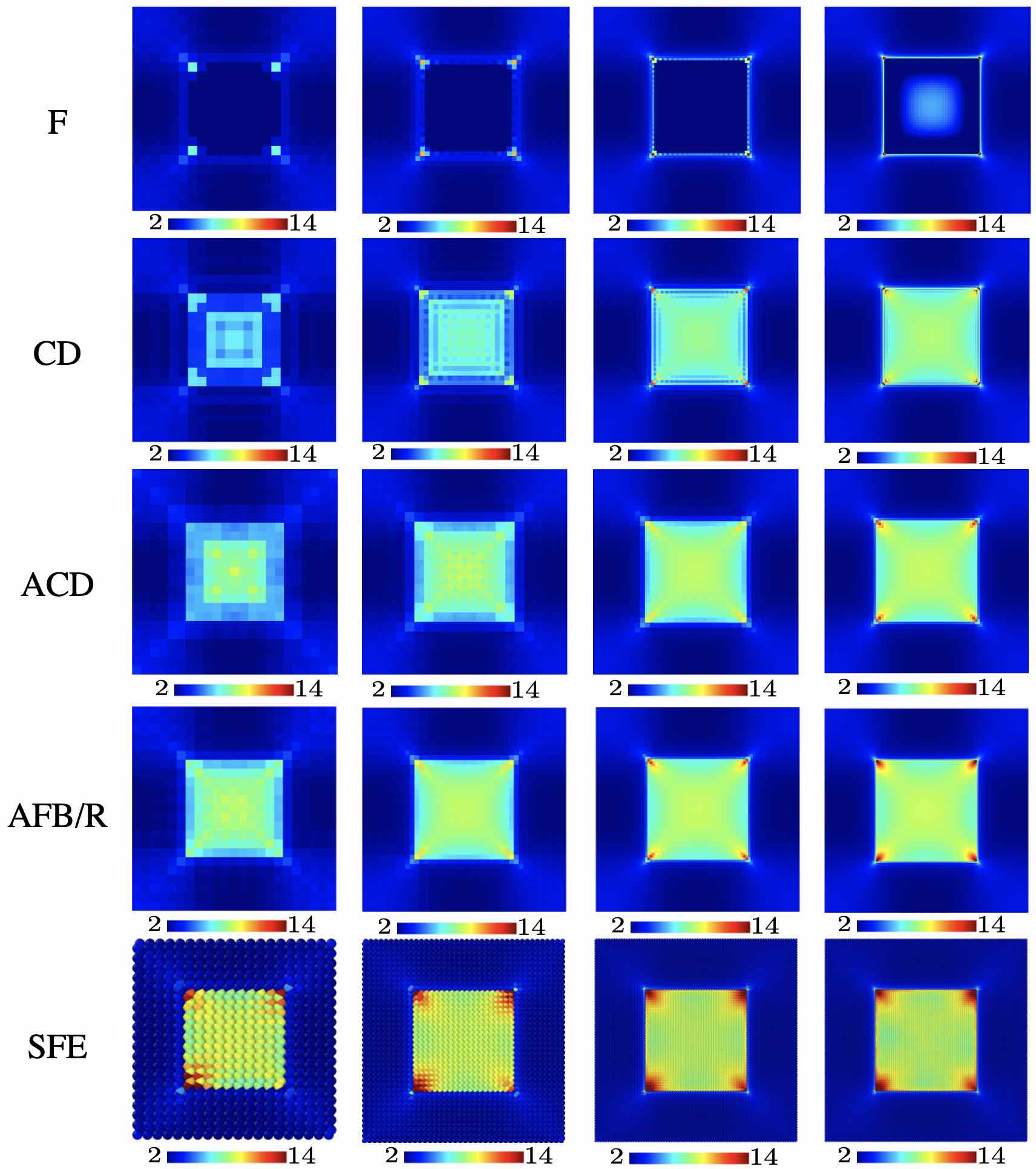
Figure 6: Comparison of discrete results for $T_{\!\smash{xy}}(x_{i_{1}},x_{i_{2}},z_{\mathrm{I}})/\mu_{\mathrm{M}}$ for a sharp MI interface with $\chi=1000$ for different choices of $a_{r},b_{r}$ in Algorithm TD2 and at different numerical resolutions $n$. In particular, $n=21$ (left), $n=41$ (middle left), $n=81$ (middle right), and $n=161$ (right). The same solutions are obtained for the even choices $n=22$ (left), $n=42$ (middle left), $n=82$ (middle right), and $n=162$ (right). The discrete results shown are from the grid points in the $(x_{1},x_{2})$ plane at $x_{i_{3}}=z_{\mathrm{I}}$ inside the inclusion and adjacent to the MI interface.

The analogous results for $T_{\!xy}$ at a smooth MI interface are shown in Figure 7.

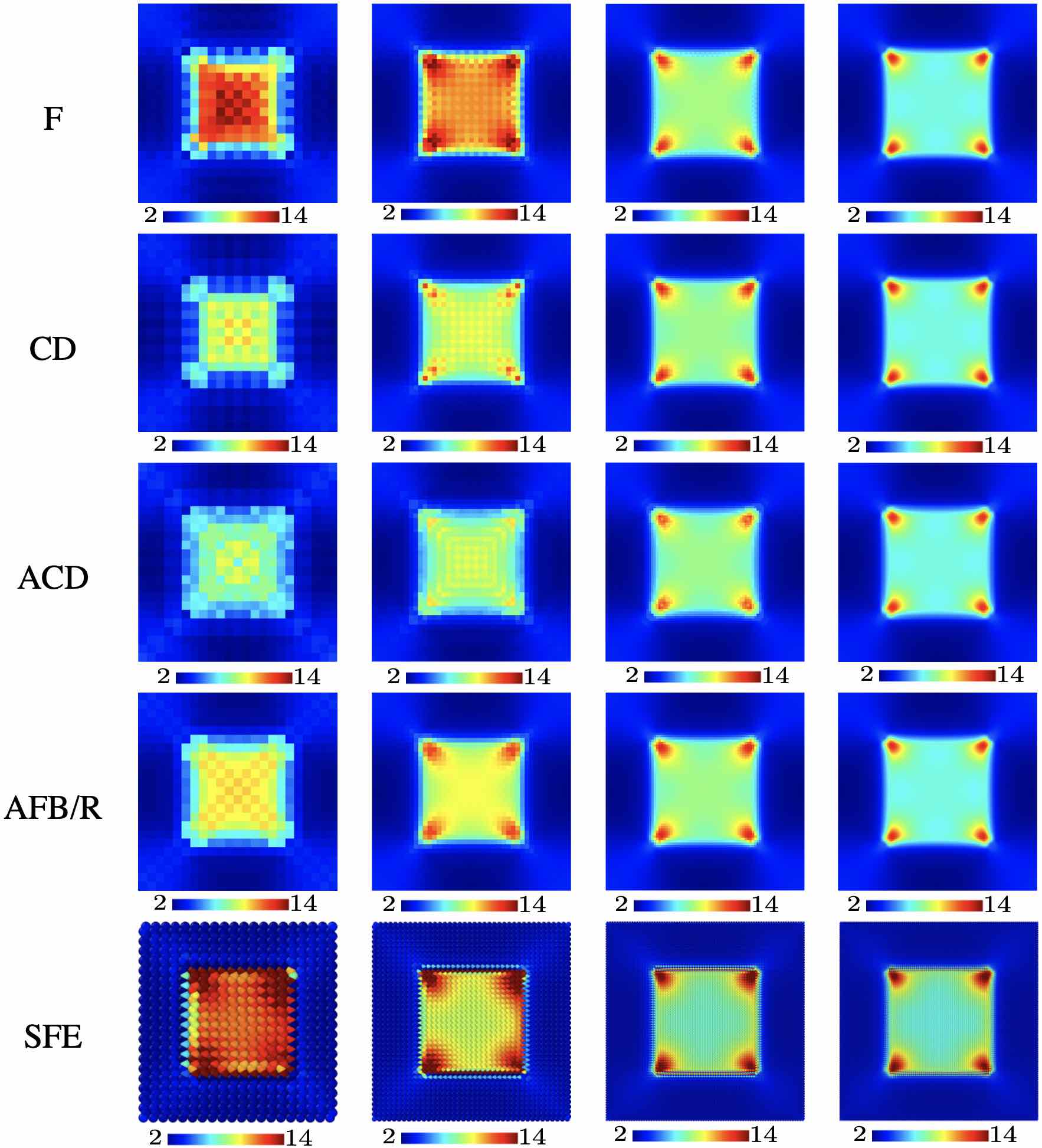
Figure 7: Same as Figure 6 for a smooth MI interface. Here, $T_{\!\smash{xy}}(x_{i_{1}},x_{i_{2}},z_{\mathrm{MI}})/\mu_{\mathrm{M}}$ is shown from the grid points in the $(x_{1},x_{2})$ plane on the MI interface at $x_{i_{3}}=z_{\mathrm{MI}}$. As in the 1D case and Figure 3, the smooth transition in stiffness between matrix and inclusion is based on $\epsilon/l=1/100$ in each direction.

As seen in Figure 6 (top row), for the discontinuous MI interface case in the context of (45), the choice $a_{r}=\mathrm{F}$ yields qualitatively incorrect results at the resolutions considered. Indeed, as shown by Willot (2015, Figure 4), who worked with much finer discretizations of $L=256,512,1024$, this choice yields correct results for this benchmark case only at much higher resolution. In contrast, the central difference choice $a_{r}=\mathrm{CD}$ (Figure 6, second row from the top) yields a stress field which is qualitatively correct and nearly converges at the highest resolution investigated here. Among the choices based on conjugacy (45), $a_{r}=\mathrm{ACD}$ (Figure 6, middle row) converges almost as quickly as the non-conjugate AFB/R choice $(a_{r},b_{r})=(\mathrm{AFD},\mathrm{AhC})$ (Figure 6, second row from the bottom), which is closest to the SFE-based reference results (Figure 6, bottom row).

Analogous to the 1D case (Figure 3), and as expected, a quite different picture emerges for the convergence behavior and stress field at a smooth MI interface in 3D. Indeed, as for the 1D results in Figure 3 (right), the convergence behavior displayed in Figure 7 in the 3D case for all choices of $(a_{r},b_{r})$ is affected predominantly by numerical resolution. In particular, as in the discontinuous MI interface case, among the choices based on conjugacy (45), $a_{r}=\mathrm{ACD}$ converges almost as quickly as the non-conjugate AFB/R choice $(a_{r},b_{r})=(\mathrm{AFD},\mathrm{AhC})$, which again is closest to the SFE-based reference case (bottom row).

As evident in the results from Figures 6 and 7, the stress field at the MI corners is most sensitive to numerical resolution. To look at this in more detail, consider the results in Figure 8.

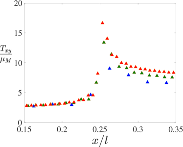
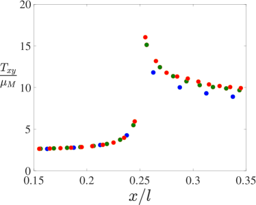
Figure 8: Discrete AFB/R (left, triangles) and SFE (right, circles) results for $T_{\!xy}(x_{i_{1}},y_{\mathrm{I}},z_{\mathrm{I}})$ across a MI corner for the sharp (left) MI interface. Results shown are at grid points in the $x_{1}$ direction for fixed $x_{i_{2}}=y_{\mathrm{I}},x_{i_{3}}=z_{\mathrm{I}}$ just inside the inclusion and for the numerical resolutions of $n_{r}=42$ (blue), $n_{r}=82$ (green), $n_{r}=162$ (red).

As expected, in the sharp interface case, the solution does not converge with increasing resolution, i.e., is mesh-dependent, in contrast to the smooth interface case. The convergence behavior of the ACD ($a_{r}=\mathrm{ACD}$) algorithm based on conjugacy (45), as well the AFB/R ($(a_{r},b_{r})=(\mathrm{AFD},\mathrm{AhC})$), are compared for both the sharp and smooth MI interfaces are compared in Figure 9.

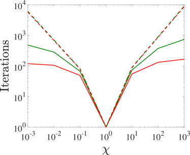
Figure 9: Convergence behavior of selected algorithms as a function of phase contrast at sharp (solid curves) and smooth (dashed curves) MI interfaces for $n_{r}=161,162$. Red: AFB/R. Green: $a_{r}=\mathrm{ACD}$. No convergence results for $a_{r}=\mathrm{F}$ are shown because this case does not converge in less than $10^{4}$ iterations at the highest contrasts.

As shown, for phase contrasts up to a factor of 10 (i.e., $\chi=10^{-1},10^{1}$), little difference in convergence rate is apparent. For higher contrasts, however, the effect of oscillations due to Gibbs and aliasing on the convergence rate for the sharp interface cases becomes apparent. Indeed, as expected from the stress results in Figure 6, the effective low-pass filtering effect of finite-difference discretization of differential operators for $a_{r}=\mathrm{ACD}$ and AFB/R reduces the effect of oscillations due to Gibbs and aliasing on convergence rate. In particular, for high phase contrasts, the convergence rate for AFB/R at $n_{r}=161,162$ is about $10^{2}$ times faster than for $a_{r}=\mathrm{F}$, and about 5 times faster than for $a_{r}=\mathrm{ACD}$, for the current benchmark case.

6.2 Results based on piecewise-constant discretization

Lastly, results from Algorithm PCD2 for $(a_{r},b_{r})=(\mathrm{AFD},\mathrm{AhC})$ (i.e., AFB/R) are compared with corresponding ones from Algorithm DGO2 in Figure 10.

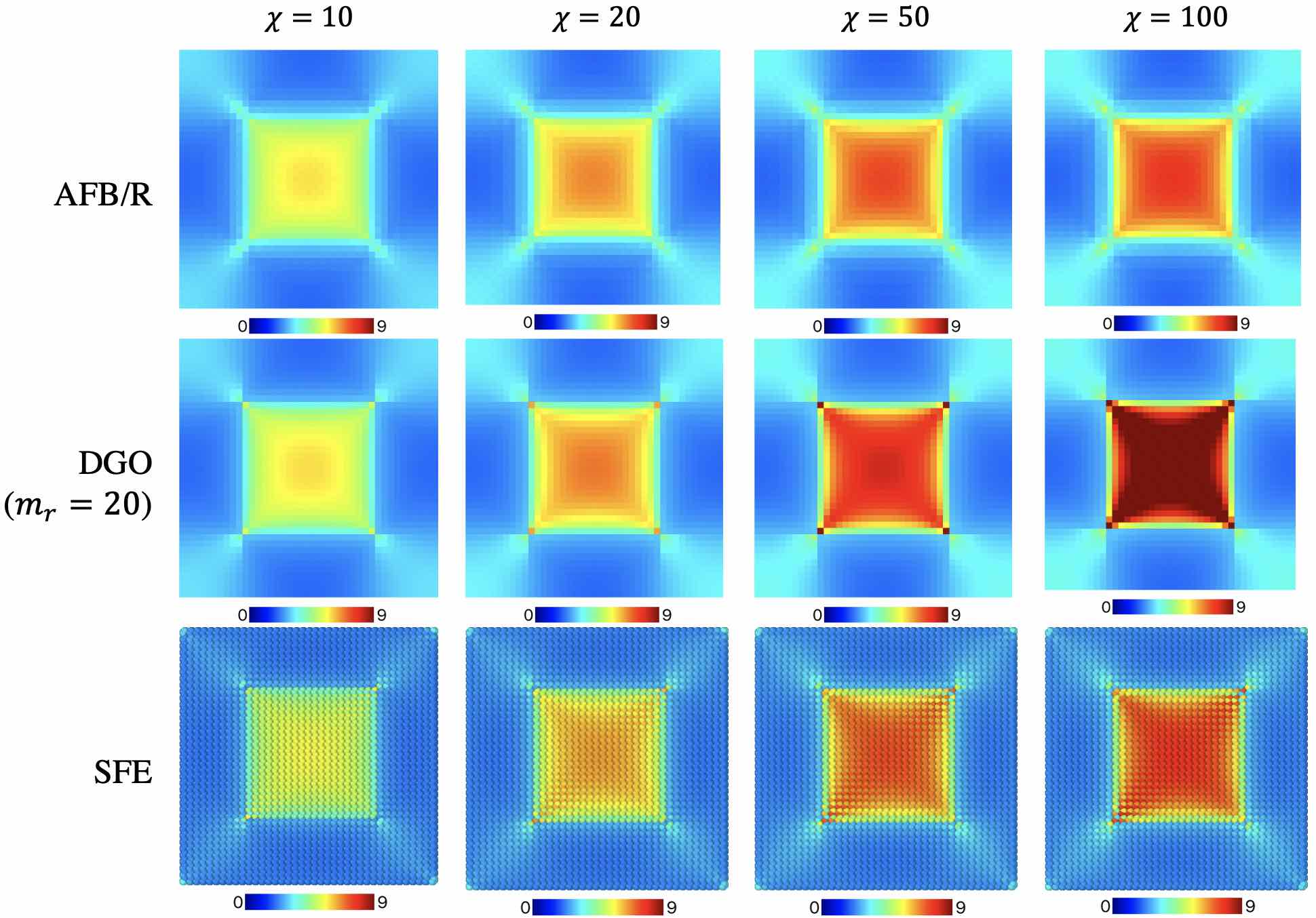
Figure 10: PCD-based results from AFB/R (above), the DGO (middle) for $T_{\!\smash{xy}}^{\mathrm{c}}(x_{\smash{i_{1}}}^{\mathrm{c}},x_{\smash{i_{2}}}^{\mathrm{c}},z_{\mathrm{I}}^{\mathrm{c}})/\mu_{\mathrm{M}}$ and SFE (below), in the sharp MI interface case for different phase contrasts $\chi$ at a resolution of $n_{r}=40$. The discrete results shown are from the grid points in the inclusion adjacent ($x_{\smash{i_{3}}}^{\mathrm{c}}=z_{\mathrm{I}}^{\mathrm{c}}$) to the MI interface. See text for discussion.

Except for the smaller phase contrasts and consequently lower stress levels, the PCD-based results for AFB/R in Figure 10 (upper row) agree with the TD-based results in Figure 6 (middle left row). For the chosen nodal resolution of $n_{r}=40$, recall that $m_{r}=\frac{1}{2}n_{r}=20$ in AFB/R. For comparability, then, $m_{r}=20$ was chosen to obtain the DGO-based results. Except for the much higher stress at the MI corners obtained with the DGO, the results from both algorithms agree (even quantitatively) well for $\chi=10$. With increasing $\chi$, however, the solution based on the DGO is much stiffer than than based on AFB/R, indicating lack of convergence at this resolution. Consequently, the DGO converges more slowly than AFB/R in the context of PCD.

As mentioned in the introduction, in contrast to the current case of cubic inclusions, Eloh et al. (2019, §§4.3-4.4) consider spherical inclusions for which analytic solutions exist (e.g., Mura, 1987). In addition, following Anglin et al. (2014), they work with phase contrasts $\chi$ of $0.5$ and $2$ in the bulk modulus $\kappa:=(\lambda+2\mu/3)$. Recalling that $\lambda_{\mathrm{I}}=\chi\lambda_{\mathrm{M}}$ and $\mu_{\mathrm{I}}=\chi\mu_{\mathrm{M}}$ from (49), note that $\kappa_{\mathrm{I}}=\chi\,\kappa_{\mathrm{M}}$ also holds. Consequently, they worked with smaller phase contrasts than $\chi=10$ upon which the results in Figure 10 are based. Further, Eloh et al. (2019) assume $\kappa_{\mathrm{H}}=\frac{1}{2}(\kappa_{\mathrm{M}}+\kappa_{\mathrm{I}})$, $\nu_{\mathrm{H}}=\nu_{\mathrm{M}}=\nu_{\mathrm{I}}$, and $\lambda_{\mathrm{M}}/\mu_{\mathrm{M}}=5.2$, the latter in contrast to $\lambda_{\mathrm{M}}/\mu_{\mathrm{M}}=1$ assumed by Willot (2015) and here. For isotropic elastic behavior, this plays a role in normal strain control cases, but not in the current case of shear strain control.

7 Summary and discussion

In the current work, a number of algorithms have been developed and compared for the numerical solution of periodic boundary-value problems (BVPs) for the quasi-static mechanical behavior of heterogeneous linear elastic materials based on Fourier series discretization. In particular, two such discretizations are considered and compared here. The first is based on trapezoidal approximation of the integral (8)₂ over the unit cell determining the Fourier modes $\hat{f}_{\kappa}$ in the truncated Fourier series (8)₁, resulting in the trapezoidal discretization (10) of this series. The second is based on approximation of the integrand in (8)₂ as piecewise-constant, yielding the piecewise-constant discretization (21) of (8)₁. A comparison of these two implies that a basic difference between them lies in the dependence of (21) on $s_{\kappa}=\mathop{\mathrm{sinc}}(\pi\kappa/n)$. As shown by Algorithms TD1 and PCD1, despite this difference, equivalent algorithms based on TD and PCD can nevertheless be formulated via the fact that $s_{\kappa}$ is non-zero (and so can be eliminated from the algorithm). This is in contrast to the PCD (25) of (8)₁ employed by Eloh et al. (2019) and resulting in Algorithm DGO1. Indeed, the DGO ${\check{\Gamma\mkern 4.0mu}\mkern-4.0mu}{}_{\!\!\smash{\mathrm{H}\,\omega}}^{\mathrm{c}}$ from (B.13) in the latter algorithm depends explicitly on $s_{\nu n+\omega}$.

All three algorithms TD1, PCD1 and DGO1 are based on Green function preconditioning (GFP). In addition, the first two exploit finite difference discretization (FDD) of differential operators, in particular of $\nabla$ and $\mathop{\mathrm{div}}$. In the context of TD (10) and PCD (21) of fields, different FDDs for these two operators are obtained in modal form (e.g., (11)-(12) for $\nabla$) in terms of effective wavenumbers $q_{\mu}^{a}$ (for $\nabla^{a}$) and $q_{\mu}^{b}$ (for $\mathrm{div}^{b}$). Specific FDDs consider include forward ($a,b=\mathrm{FD}$), backward ($a,b=\mathrm{BD}$), central ($a,b=\mathrm{CD}$), and half central ($a,b=\mathrm{hC}$), difference, respectively. Following in particular Willot (2015), given $a$, one choice for $b$ is based on conjugacy (18). A second one is based on choosing $b$ in such a way that the discretized stress divergence is determined in the algorithm at the (displacement) nodes. For example, for the choice $a=\mathrm{FD}$, this results in $b=\mathrm{hC}$, and so the (non-conjugate) combination $(a,b)=(\mathrm{FD},\mathrm{hC})$.

Computational comparison of these algorithms is carried out in Section 4 for the matrix-inclusion benchmark case in 1D for material heterogeneity in the form of both discontinuous and smooth compliance / stiffness distributions. In the former case, as expected from Fourier series approximation of the analytic solution and series truncation (Figure 2, left), $\tilde{E}_{a}(x)$ at the sharp MI interface in Figure 3 (left) exhibits Gibbs error independent of, and no convergence with increasing, numerical resolution for all choices of $\nabla^{a}$ ($q_{\mu}^{a}$) and $\mathrm{div}^{b}$ ($q_{\mu}^{b}$) in the context of Algorithms TD1 and PCD1. On the other hand, $\tilde{E}_{a}(x)$ does converge with increasing numerical resolution at the smooth MI interface (Figure 3, right). In addition, for the sharp interface case, comparison of strain results from Algorithms TD1, PCD1 and DGO1 in Figure 5 show that the nodal results from PCD1 deviate slightly from those of the anayltic solution and the first two algorithms in the (relatively soft) matrix, with maximum deviation in the matrix next to the MI interface.

Multidimensional versions of the 1D algorithms are formulated in Section 5 via direct componentwise- and tensor-product-based generalization. In this fashion, 3D versions TD2, PCD2 and DGO2, respectively, of the 1D algorithms TD1, PCD1 and DGO1, respectively, follow directly. As in the 1D case, all three are based on GFP, and the first two on FDDs of $\nabla$ and $\mathop{\mathrm{div}}$, now in 3D. In the context of either TD (30) or PCD (46) of 3D fields, the latter are formulated in 3D via componentwise application of the 1D approaches, resulting in the FDDs $\nabla^{\mathbf{a}}$ and $\mathrm{div}^{\mathbf{b}}$ with $\mathbf{a}=(a_{1},a_{2},a_{3})$ and $\mathbf{b}=(b_{1},b_{2},b_{3})$. As in 1D, choices for $b_{r}$ given $a_{r}$ are based on conjugacy (45) and the non-conjugate stress divergence criteria, the latter yielding in particular $b_{r}=\mathrm{AhC}$ for $a_{r}=\mathrm{AFD}$ and so the "average forward-backward/rotated" FDD, i.e., AFB/R. Computational comparsions of these are presented in Section 6. Generally speaking, an increase in phase contrast results in an increase in the condition number of the algorithmic equation system being solved, resulting in slower convergence. As such, preconditioning is clearly essential to improved convergence. As shown for example in Willot (2015) and the current work (e.g., Figure 9), the combination of GFP and FDD results in significant further improvement in convergence rate and behavior over approaches based on GFP alone such as the DGO of Eloh et al. (2019).

In the current work, the focus has been on material inhomogeneity with respect to elastic stiffness. Generalization of the current algorithms to the case of such heterogeneity with respect to both elastic stiffness and residual strain (e.g., due to lattice mismatch between phases) is straightforward. In the 3D case, the corresponding generalization $\bm{T}=\mathsfbfit{C}[\bm{E}-\bm{E}_{\ast}]$ of the stress-strain relation (with $\mathsfbfit{C}(\bm{x})$ and $\bm{E}_{\ast}(\bm{x})$ known) induces changes in the algorithms. For example, this results in the change of $\mathbf{T}_{\smash{i}}^{(0)}=\textsf{C}_{\smash{i}}\bar{\mathbf{E}}$ to $\mathbf{T}_{\smash{i}}^{(0)}=\textsf{C}_{\smash{i}}[\bar{\mathbf{E}}-\mathbf{E}_{\ast\smash{i}}]$ in the TD-based algorithm TD2. Likewise, $\mathbf{T}_{\smash{i}}^{\mathrm{c}(0)}=\textsf{C}_{\smash{i}}^{\mathrm{c}}\bar{\mathbf{E}}$ generalizes to $\mathbf{T}_{\smash{i}}^{\mathrm{c}(0)}=\textsf{C}_{\smash{i}}^{\mathrm{c}}[\bar{\mathbf{E}}-\mathbf{E}_{\ast\smash{i}}^{\mathrm{c}}]$ in the PCD-based algorithms PCD2 and DGO2.

In the context of strong mechanical equilbrium, a displacement-based approach related to the current one has quite recently been developed by Lucarini and Segurado (2019). They refer to this approach as displacement-based FFT (DBFFT). As the name implies, they also work with the displacement as the primary discretant and the split (29). In particular, their algorithm is based on quasi-static mechanical equilibrium in Fourier space in the form $\hat{\bm{A}}(\bm{q})\,\hat{\bm{u}}^{\mathrm{p}}=\hat{\mathsfbfit{C}}[\bar{\bm{E}}]\bm{q}$ for $\bm{q}\neq\bm{0}$ in terms of the generalized acoustic tensor $\hat{\bm{A}}(\bm{q})\,\hat{\bm{v}}:=-\mathcal{F}\{\mathsfbfit{C}[\mathcal{F}^{-1}\{\hat{\bm{v}}\otimes\bm{q}\}]\}\bm{q}$. As noted by them, Fourier discretization and real-function-based reduction yields a discrete system for displacement based on a full-rank associated Hermitian matrix. In turn, this facilitates use of preconditioners. In the current context, their choice corresponds in particular to those $\textsf{C}_{\mathrm{H}}=\bar{\textsf{C}}$ and $(a_{r},b_{r})=(\mathrm{F},\mathrm{F})$ in (33). In terms of Fourier transforms, this results in $\hat{\bm{G}}_{\smash{\mathrm{H}}}^{-1}(\bm{q})\,\bm{a}=-\bar{\mathsfbfit{C}}[\bm{a}\otimes\bm{q}]\bm{q}$ for $\bm{q}\neq\bm{0}$. Algorithmic extension of this to $\bm{q}=\bm{0}$ then results in a preconditioning operator $\hat{\bm{M}}(\bm{q})$ which approximately inverts $\hat{\bm{A}}(\bm{q})$ for use in iterative numerical solution.

Traditional (i.e., linear elastic) micromechanics based on a (linear) stress-strain relation $\bm{T}(\bm{E})$ treats the (linear) strain $\bm{E}$ (and not displacement) as the primary unknown. In the computational context, this translates into the treatment of $\bm{E}$, or more recently in the geometrically non-linear case, the deformation gradient $\bm{F}$, as the primary discretant. In this case, compatibility needs to be enforced via additional algorithmic constraints. Alternatively, as discussed in the current work, one can work directly with the displacement or deformation field as the primary discretant. This is true in both the current case of strong mechanical equilibrium as well as in the case of weak mechanical equilibrium, as shown by the recent work of de Geus et al. (2017). To discuss the latter briefly here, consider weak equilibrium $\int\bm{T}(\bm{x})\cdot\bm{E}_{\mathrm{v}}(\bm{x})\ dv(\bm{x})=\int{\hat{\bm{T}\mkern 3.0mu}\mkern-3.0mu}{}(\bm{k})\cdot{\hat{\bm{E}\mkern 3.0mu}\mkern-3.0mu}{}_{\smash{\mathrm{v}}}^{\ast}(\bm{k})\ dv(\bm{k})$ (i.e., via the Rayleigh-Plancherel or power theorem: e.g., Bracewell, 2000, pp. 119-120) for any "virtual" or "test" strain field $\bm{E}_{\mathrm{v}}$. Given $\bm{H}$ compatible, ${\hat{\bm{H}\mkern 3.0mu}\mkern-3.0mu}{}_{\smash{\mathrm{v}}}^{\ast}=\hat{\bm{u}}_{\mathrm{v}}\otimes\bm{q}^{\ast}$ holds, again with $\bm{q}=\imath\bm{k}$. Then $\hat{\bm{u}}_{\mathrm{v}}={\hat{\bm{H}\mkern 3.0mu}\mkern-3.0mu}{}_{\smash{\mathrm{v}}}^{\ast}\bm{q}/|\bm{q}|^{2}$ for $\bm{q}\neq\bm{0}$, inducing in turn ${\hat{\bm{T}\mkern 3.0mu}\mkern-3.0mu}{}\cdot\hat{\bm{E}}_{\smash{\mathrm{v}}}^{\ast}=\mathsfbfit{P}_{\bm{H}}\,{\hat{\bm{T}\mkern 3.0mu}\mkern-3.0mu}{}\cdot{\hat{\bm{H}\mkern 3.0mu}\mkern-3.0mu}{}_{\smash{\mathrm{v}}}^{\ast}$ with $\mathsfbfit{P}_{\bm{H}}:=\bm{I}\,\square\,(\bm{q}\otimes\bm{q}^{\ast})/|\bm{q}|^{2}$. Consequently, the projection $\mathsfbfit{P}_{\bm{H}}$ enforces compatibility when $\bm{H}$ is the primary discretant and unknown. Alternatively, as done in the current work, one can simply work directly with the displacement field or the deformation field as the primary discretant.

Acknowledgements. Financial support of Subproject M03 of the Transregional Collaborative Research Center SFB/TRR 136 by the German Science Foundation (DFG) is gratefully acknowledged.

Appendix A Trapezoidal approximation / discretization

Note that the trapezoidal discretization $\hat{f}_{\smash{\kappa}}^{\mathrm{t}}$ of $\hat{f}_{\smash{\kappa}}$ in (9) satisfies cardinality

$$\begin{array}[]{rclclclcl}\displaystyle\sum\nolimits_{\kappa=-m}^{m}e^{\imath k_{\kappa}x_{i}}\hat{f}_{\kappa}^{\mathrm{t}}&=&\displaystyle\sum\nolimits_{j=1}^{n}\sum\nolimits_{\kappa=-(n-1)/2}^{(n-1)/2}n^{-1}e^{2\pi\imath\kappa(i-j)/n}f(x_{\!j})&=&\displaystyle\sum\nolimits_{j=1}^{n}\delta_{ij}f(x_{\!j})&=&f(x_{i})\,,\\[5.69054pt] \displaystyle\sum\nolimits_{\kappa=-m+1}^{m}e^{\imath k_{\kappa}x_{i}}\hat{f}_{\kappa}^{\mathrm{t}}&=&\displaystyle\sum\nolimits_{j=1}^{n}\sum\nolimits_{\kappa=-n/2+1}^{n/2}n^{-1}e^{2\pi\imath\kappa(i-j)/n}\,f(x_{\!j})&=&\displaystyle\sum\nolimits_{j=1}^{n}\delta_{ij}f(x_{\!j})&=&f(x_{i})\,,\\[5.69054pt] \displaystyle\sum\nolimits_{\kappa=-m}^{m-1}e^{\imath k_{\kappa}x_{i}}\hat{f}_{\kappa}^{\mathrm{t}}&=&\displaystyle\sum\nolimits_{j=1}^{n}\sum\nolimits_{\kappa=-n/2}^{n/2-1}n^{-1}e^{2\pi\imath\kappa(i-j)/n}\,f(x_{\!j})&=&\displaystyle\sum\nolimits_{j=1}^{n}\delta_{ij}f(x_{\!j})&=&f(x_{i})\,,\end{array}$$ (A.1)

(i.e., the interpolation condition) for both $n$ odd ($m=(n-1)/2$) and $n$ even ($m=n/2$). Given these,

$$\mathcal{I}_{\!n\,}^{\mathrm{o}}f(x):=\sum\nolimits_{\kappa=-(n-1)/2}^{(n-1)/2}e^{\imath k_{\kappa}x}\hat{f}_{\kappa}^{\mathrm{t}}$$ (A.2)

for $n$ odd, and

$$\mathcal{I}_{\!n\,}^{\mathrm{e}}f(x):=\sum\nolimits_{\kappa=-n/2}^{n/2-1}e^{\imath k_{\kappa}x}\hat{f}_{\kappa}^{\mathrm{t}}=\sum\nolimits_{\kappa=-n/2+1}^{n/2}e^{\imath k_{\kappa}x}\hat{f}_{\kappa}^{\mathrm{t}}$$ (A.3)

for $n$ even, interpolate $f(x)$. Note that the second form of (A.3) is employed for example by Willot (2015, Equations (10)-(12)).

For Fourier discretization based on (9), the index transformations

$$\begin{array}[]{rclcrclcl}\kappa&\mapsto&\mu=\kappa+1+m&\colon&\{-m,\ldots,m\}&\to&\{1,\ldots,n\}\,,&&\hbox{$m=\frac{1}{2}(n-1)$, $n$ odd}\,,\\ \kappa&\mapsto&\mu=\kappa+1+m&\colon&\{-m,\ldots,m-1\}&\to&\{1,\ldots,n\}\,,&&\hbox{$m=\frac{1}{2}n$, $n$ even}\,,\\ \kappa&\mapsto&\mu=\kappa+m&\colon&\{-m-1,\ldots,m\}&\to&\{1,\ldots,n\}\,,&&\hbox{$m=\frac{1}{2}n$, $n$ even}\,,\end{array}$$ (A.4)

are useful. Restricting attention to the first two, define

$$q_{\mu}:=\imath k_{\mu-1-m}\,,\quad\varphi_{\mu}(x):=n^{-1/2}e^{q_{\mu}x}\,,\quad\check{f}_{\mu}^{\mathrm{t}}:=n^{-1/2}\sum\nolimits_{i=1}^{n}e^{-q_{\mu}x_{i}}f(x_{i})\,.$$ (A.5)

Based on these, (A.2) and (A.3)₂ take the common form

$$\mathcal{I}_{\!n\,}f(x)=\sum\nolimits_{\mu=1}^{n}\varphi_{\mu}(x)\,\check{f}_{\mu}^{\mathrm{t}}\,,$$ (A.6)

with $\check{f}_{\smash{\mu}}^{\mathrm{t}}=\sum\nolimits_{i=1}^{n}F_{\!\smash{\mu i}\,}^{\mathrm{t}-}f(x_{i})$, $f(x_{i})=\sum\nolimits_{\mu=1}^{n}F_{\!\smash{\mu i}\,}^{\mathrm{t}+}\check{f}_{\smash{\mu}}^{\mathrm{t}}$, and

$$F_{\!\smash{\mu i}\,}^{\mathrm{t}\pm}:=n^{-1/2}e^{\pm q_{\mu}x_{i}}=n^{-1/2}e^{\pm 2\pi\imath(\mu-1-m)(i-1)/n}\,,\quad m=\left\{\begin{array}[]{lcl}\frac{1}{2}(n-1)&&\hbox{$n$ odd}\\ \frac{1}{2}n&&\hbox{$n$ even}\end{array}\right.\,.$$ (A.7)

Note that $\varphi_{\mu}(x_{i})=F_{\!\smash{\mu i}\,}^{+}$ and $\sum_{\mu=1}^{n}\!F_{\!\smash{\mu i}\,}^{\mathrm{t}+}F_{\!\smash{\mu\!j}\,}^{\mathrm{t}-}=\delta_{i\!j}$, consistent with cardinality.

Appendix B Piecewise-constant approximation / discretization

The form $\hat{f}_{\kappa}^{\mathrm{c}}$ for $\hat{f}_{\kappa}$ from (20) in the case of piecewise-constant $f(x)$ determines the corresponding Fourier series discretization

$$\mathcal{F}_{\!\!n}^{\mathrm{c}}f(x):=\sum\nolimits_{\mu=1}^{n}\varphi_{\mu}^{\mathrm{c}}(x)\,\check{f}_{\mu}^{\mathrm{c}}\,,\quad f(x_{i}^{\mathrm{c}})=\sum\nolimits_{\mu=1}^{n}F_{\!\smash{\mu i}\,}^{\mathrm{c}+}\check{f}_{\mu}^{\mathrm{c}}\,,\quad\check{f}_{\mu}^{\mathrm{c}}=\sum\nolimits_{i=1}^{n}F_{\!\smash{\mu i}\,}^{\mathrm{c}-}f(x_{i}^{\mathrm{c}})\,,$$ (B.8)

via (A.4)_1,2. Here, $\varphi_{\smash{\mu}}^{\mathrm{c}}(x):=n^{-1/2}s_{\smash{\mu}}^{\mathrm{c}}\,e^{q_{\smash{\mu}}x}$, $s_{\smash{\mu}}^{\mathrm{c}}:=s_{\smash{\mu-1-m}}$ and $F_{\!\smash{\mu i}\,}^{\mathrm{c}\pm}:=n^{-1/2}e^{\pm q_{\mu}x_{i}^{\mathrm{c}}}$. Since $s_{\smash{\mu}}^{\mathrm{c}}\neq 1$ for $\mu\neq m+1$, note that

$$\mathcal{F}_{\!\!n}^{\mathrm{c}}f(x_{i}^{\mathrm{c}})=\sum\nolimits_{\mu=1}^{n}\varphi_{\mu}^{\mathrm{c}}(x_{i}^{\mathrm{c}})\,\check{f}_{\mu}^{\mathrm{c}}=\sum\nolimits_{j=1}^{n}\sum\nolimits_{\mu=1}^{n}s_{\mu}^{\mathrm{c}}F_{\!\smash{\mu i}\,}^{\mathrm{c}+}F_{\!\mu\!j\,}^{\mathrm{c}-}f(x_{\!j}^{\mathrm{c}})\approx f(x_{i}^{\mathrm{c}})$$ (B.9)

is only approximately cardinal. In the approach of Eloh et al. (2019) also based on (20), approximate cardinality takes the form

$$f(x_{i}^{\mathrm{c}})\approx\mathcal{F}_{\!\!p\,}^{\mathrm{c}}f(x_{i}^{\mathrm{c}})=n^{-1/2}\sum\nolimits_{\omega=0}^{n-1}e^{\imath k_{\omega}x_{i}^{\mathrm{c}}}\sum\nolimits_{\nu=-m}^{m-1}(-1)^{\nu}s_{\nu n+\omega}\,\check{f}_{\nu n+\omega}^{\mathrm{c}}$$ (B.10)

via (25) and $e^{-\imath k_{\nu n}x_{i}^{\mathrm{c}}}=e^{-2\pi\imath\nu(i-\frac{1}{2})}=e^{\pi\imath\nu}e^{-2\pi\imath\nu i}=(-1)^{\nu}$ ($p=nm$ even). Comparison of (B.10) and (26)₂ results in

$$\check{f}_{\omega}^{\mathrm{c}}\approx\sum\nolimits_{\nu=-m}^{m-1}(-1)^{\nu}s_{\nu n+\omega}\,\check{f}_{\nu n+\omega}^{\mathrm{c}}\,,\quad\sum\nolimits_{\nu=-m\atop\nu\neq 0}^{m-1}(-1)^{\nu}s_{\nu n}\,\check{f}_{\nu n}^{\mathrm{c}}\approx 0\,,$$ (B.11)

via the fact that $\bar{f}=n^{-1/2}\check{f}_{0}^{\mathrm{c}}=n^{-1}\sum\nolimits_{i=1}^{n}f(x_{i}^{\mathrm{c}})$ from (1)₂, (8)₂ and (20)₃. Given (B.11), note that (B.10) reduces to $\tilde{f}(x_{i}^{\mathrm{c}})\approx\sum\nolimits_{\omega=1}^{n-1}e^{\imath k_{\omega}x_{i}^{\mathrm{c}}}\sum\nolimits_{\nu=-m}^{m-1}(-1)^{\nu}s_{\nu n+\omega}\,\check{f}_{\nu n+\omega}$ for the fluctuation part $\tilde{f}(x_{i}^{\mathrm{c}})$ of $f(x_{i}^{\mathrm{c}})=\bar{f}+\tilde{f}(x_{i}^{\mathrm{c}})$ in the context of (1).

As done by Eloh et al. (2019), the principle application of these relations and in particular of (B.11)₁ is to obtain the discretization

$${\check{\Gamma\mkern 4.0mu}\mkern-4.0mu}{}_{\!\!\mathrm{H}\omega}^{\mathrm{c}}\check{T}_{\!\smash{\omega}}^{\mathrm{c}}=0\,,\quad\omega=1,\ldots,n-1\,,$$ (B.12)

of (28) in terms of the "discrete Green operator" (DGO)

$${\check{\Gamma\mkern 4.0mu}\mkern-4.0mu}{}_{\!\!\mathrm{H}\omega}^{\mathrm{c}}:=\sum\nolimits_{\nu=-m}^{m-1}s_{\nu n+\omega}\ {\hat{\Gamma\mkern 4.0mu}\mkern-4.0mu}{}_{\!\!\mathrm{H}}(k_{\nu n+\omega})\,,\quad\omega=1,\ldots,n-1\,.$$ (B.13)

Both (B.12) and (B.13) are employed in Algorithm DGO1, and via (Cartesian) tensor product generalization in Algorithm DGO2.

References

- Anglin et al. (2014) Anglin, B. S., Lebensohn, R. A., Rollett, A. D., 2014. Validation of a numerical method based on fast Fourier transforms for heterogeneous thermoelastic materials by comparison with analytical solutions. Computational Materials Science 87, 209–217.
- Bracewell (2000) Bracewell, R. N., 2000. The Fourier Transform and Its Application, 3rd Edition. McGraw-Hill.
- Brisard and Dormieux (2010) Brisard, S., Dormieux, L., 2010. FFT-based methods for the mechanics of composites: a general variational framework. Computational Materials Science 49, 663–671.
- Brown et al. (2002) Brown, C. M., Dreyer, W., Müller, W., 2002. Discrete fourier transforms and their application to stress-strain problems in composite mechanics: a convergence study. Proceedings of the Royal Society of London A 458, 1967–1987.
- Canuto et al. (1988) Canuto, C., Hussaini, M. Y., Quateroni, A., Zang, T. A., 1988. Spectral Methods in Fluid Dynamics. Springer Series in Computational Physics. Springer-Verlag, Berlin.
- Chen (2002) Chen, L.-Q., 2002. Phase-field model for microstructure evolution. Annual Review of Material Research 32, 113–140.
- de Geus et al. (2017) de Geus, T. W. J., Vondřejc, J., Zeman, J., Peerlings, R. H. J., Geers, M. G. D., 2017. Finite strain FFT-based non-linear solvers made simple. Computer Methods in Applied Mechanics and Engineering 318, 412–430.
- Djaka et al. (2017) Djaka, K. S., Villani, A., Taupin, V., Capolungo, L., Berbenni, S., 2017. Field Dislocation Mechanics for heterogeneous elastic materials: a numerical spectral approach. Computer Methods in Applied Mechanics and Engineering 315, 921–942.
- Dreyer and Müller (2000) Dreyer, W., Müller, W., 2000. A study of the coarsening of tin/lead solders. International Journal of Solids and Structures 37, 3841–3871.
- Eisenlohr et al. (2013) Eisenlohr, P., Diehl, M., Lebensohn, R. A., Roters, F., 2013. A spectral method solution to crystal elasto viscoplasticity at finite strains. International Journal of Plasticity 46, 37–53.
- Eloh et al. (2019) Eloh, K. S., Jacques, A., Berbenni, S., 2019. Development of a new consistent discrete Green operator for FFT- based methods to solve heterogeneous problems with eigenstrains. International Journal of Plasticity 116, 1–23.
- Eyre and Milton (1999) Eyre, D. J., Milton, G. W., 1999. A fast numerical scheme for computing the response of composites using grid refinement. The European Physical Journal 6, 41–47.
- Gottlieb and Orszag (1977) Gottlieb, D., Orszag, S. A., 1977. Numerical Analysis of Spectral Methods: Theory and Application. SIAM, Philadelphia.
- Kabel et al. (2014) Kabel, M., Böhlke, T., Schneider, M., 2014. Efficient fixed point and Newton-Krylov solvers for FFT-based homogenization of elasticity at large deformations. Computational Mechanics 54, 1497–1514.
- Khachaturyan (1983) Khachaturyan, A. G., 1983. Theory of Structural Transformations in Solids. Wiley, New York.
- Kopriva (2009) Kopriva, D. A., 2009. Implementing Spectral Methods for Partial Differential Equations. Springer.
- Lebensohn (2001) Lebensohn, R. A., 2001. N-site modeling of a 3d viscoplastic polycrystal using Fast Fourier Transform. Acta Materialia 49, 2723–2737.
- Lebensohn and Rollett (2020) Lebensohn, R. A., Rollett, A. D., 2020. Spectral methods for full-field micromechanical modelling of polycrystalline materials. Computational Materials Science 173, 109336.
- Liu (2011) Liu, S. H., 2011. Numerical Analysis of Partial Differential Equations. Wiley.
- Lucarini and Segurado (2019) Lucarini, S., Segurado, J., 2019. DBFFT: a displacement based FFT approach for non-linear homogenization of the mechanical behavior. International Journal of Engineering Science 144, 103131.
- Michel et al. (2000) Michel, J. C., Moulinec, H., Suquet, P., 2000. A computational method based on augmented Lagrangians and Fast Fourier Transforms for composites with high contrast. Computational Modelling in Engineering Science 1, 79–88.
- Michel et al. (2001) Michel, J. C., Moulinec, H., Suquet, P., 2001. A computational scheme for linear and non-linear composites with arbitrary phase contrast. International Journal of Numerical Methods in Engineering 52, 139–160.
- Mishra et al. (2016) Mishra, N., Vondřejc, J., Zeman, J., 2016. A comparative study on low-memory iterative solvers for FFT-based homogenization of periodic media. Journal of Computational Physics 321, 151–168.
- Moulinec and Silva (2014) Moulinec, H., Silva, F., 2014. Comparison of three accelerated FFT-based schemes for computing the mechanical response of composite materials. International Journal for Numerical Methods in Engineering 97, 960–985.
- Moulinec and Suquet (1994) Moulinec, H., Suquet, P., 1994. A fast numerical method for computing the linear and nonlinear mechanical properties of composites. Comptes Rendus de l’Académie des Sciences Paris 318, 1417–1423.
- Mura (1987) Mura, T., 1987. Micromechanics of Defects in Solids. Martinus Nijhoff, Dordrecht.
- Nemat-Nasser and Hori (1999) Nemat-Nasser, S., Hori, M., 1999. Micromechanics: Overall Properties of Heterogeneous Materials. Elsevier.
- Press et al. (2007) Press, W. H., Teukolsky, S. A., Vetterling, W. T., Flannery, B. P., 2007. Numerical Recipies: The Art of Scientific Computing, Third Edition. Cambridge University Press.
- Schneider et al. (2017) Schneider, M., Merkert, D., Kabel, M., 2017. FFT-based homogenization for microstructures discretized by linear hexahedral elements. International Journal for Numerical Methods in Engineering 109, 1461–1489.
- Shanthraj et al. (2015) Shanthraj, P., Eisenlohr, P., Diehl, M., Roters, F., 2015. Numerically robust spectral methods for crystal plasticity simulations of heterogeneous materials. International Journal of Plasticity 66, 31–45.
- Suquet (1997) Suquet, P., 1997. Continuum Micromechanics. Vol. 377 of CISM International Center for Mechanical Sciences. Springer, Berlin.
- Trefethen (2000) Trefethen, L. N., 2000. Spectral Methods in MATLAB. SIAM.
- Willot (2015) Willot, F., 2015. Fourier-based schemes for computing the mechanical response of composites with accurate local fields. Comptes Rendus Mécanique 343, 232–245.