Modeling and Analysis of Dynamic Charging for EVs: A Stochastic Geometry Approach

Abstract

With the increasing demand for greener and more energy efficient transportation solutions, electric vehicles (EVs) have emerged to be the future of transportation across the globe. However, currently, one of the biggest bottlenecks of EVs is the battery. Small batteries limit the EVs driving range, while big batteries are expensive and not environmentally friendly. One potential solution to this challenge is the deployment of charging roads, i.e., dynamic wireless charging systems installed under the roads that enable EVs to be charged while driving. In this paper, we use tools from stochastic geometry to establish a framework that enables evaluating the performance of charging roads deployment in metropolitan cities. We first present the course of actions that a driver should take when driving from a random source to a random destination in order to maximize dynamic charging during the trip. Next, we analyze the distribution of the distance to the nearest charging road. This distribution is vital for studying multiple performance metrics such as the trip efficiency, which we define as the fraction of the total trip spent on charging roads. Next, we derive the probability that a given trip passes through at least one charging road. The derived probability distributions can be used to assist urban planners and policy makers in designing the deployment plans of dynamic wireless charging systems. In addition, they can also be used by drivers and automobile manufacturers in choosing the best driving routes given the road conditions and level of energy of EV battery.

I Introduction

As the global trend towards sustainable energy has significantly transformed several industries, automobile manufacturing is not an exception. Almost every major car manufacturer now has models that run entirely on electric batteries. It is expected that in the next decades, electric vehicles (EVs) will account for a large portion of total car production [1].

Although there are several challenges with EVs, e.g., engines, sensors, one of the biggest bottlenecks of EVs is the battery [2]. Ideally, batteries for EVs should last for a comparable distance compared to gasoline tanks. The battery should also be quickly charged and remain in good condition after thousands of charging cycles. Moreover, it should be affordable and finally, be environment-friendly. However, there are a couple of important trade-offs with the current EVs batteries that need to be considered [3]. For example, large-capacity batteries, which are optimized for driving distance, are expensive to make, slow to charge, and not friendly to the environment. On the other hand, small-capacity batteries are more affordable but require more frequent charging.

There have been steady advances in producing batteries that fit the demand [4]. However, as batteries require charging, we still need solutions on how to charge them effectively and efficiently. In the literature, several works have been presented about optimally deploying charging stations [5, 6, 7, 8]. Although this solution seems to extend the driving range of EVs, one major drawback of charging stations is the waiting time, especially in metropolitan cities. For example, during rush hours, charging stations may not meet the charging demand if each EV needs half an hour or more to charge. As the frequency of people using EVs in their daily commute increases, a better solution that benefits all commuters is dynamic wireless vehicle charging systems [9, 10], i.e, roads that are able to charge EVs while driving without the need to stop. Charging roads are equipped with wireless power transfer technology that enables complete wireless charging [11, 12]. This technology has been thoroughly researched in several research institutes around the world such as KAIST (Korea) [13], University of Auckland (UoA - New Zealand) [14], and Oak Ridge National Laboratory (ORNL - United States) [15]. At KAIST, since 2009, researchers have introduced six generations of dynamic wireless charging systems for both driving vehicles and stationary EVs with improved charging efficiency in each new generation [16]. UoA has been active in designing coil structure and layout for dynamic charging systems [14, 17]. ORNL has focused on integrated wireless charging systems for vehicles. They have tested their systems in a few popular car models [15, 18] and achieved good power transfer efficiency [19]. Samples of dynamic electric vehicular charging systems have also been demonstrated by QualComm Halo [20], and later by WiTricity [21]. Given the prominent future of dynamic charging technology, there is a high demand for efficiently utilizing charging roads and assessing the impact of its deployment at large scale, i.e., city level. While there are several studies on exploiting charging roads, e.g., optimizing routing policies for EVs in a specific city [22, 23], researches on modeling the impact of dynamic charging on a generic city have not been comprehensively carried out.

Motivated by the great potential of charging roads, as explained above, we study the system-level modeling and analysis of large-scale deployment of charging roads in metropolitan cities. Our goal is to provide an analytical framework that could be useful to urban planners, city policy makers, car manufacturers, and drivers. To be more precise, we consider a setup in which a fraction of the total number of roads is equipped with wireless charging capabilities. The proposed framework relies on considering a generic city, with respect to the density of roads and the fraction of charging roads. This, in turns, extends the applicability of the proposed framework, compared to a well-planned deployment scenario which only works for specific cities. Given a randomly located source and a randomly located destination, we analyze two metrics: (i) the probability that any given trip passes through at least one charging road, and (ii) the distribution of the distance from the source to the nearest charging road. These two metrics are crucial for city planners and policymakers to evaluate how effective and efficient the deployment of the charging roads is, as demonstrated in more details in Sec. III-C.

To compute the two metrics, we adopt a policy that a driver will take given a source and a destination. Since routing with charging roads is a new research topic with few published studies, we select a general and intuitive driving policy. We assume that the driver will always choose the shortest route, as this assumption has been frequently used in several routing applications on road networks [24, 25, 26]. In addition, if there are multiple shortest routes, we go on to assume that the driver will always choose the one that maximizes the time spent on charging roads. Note that this policy can be combined with more sophisticated constraints to model different EVs routing scenarios. For example, EVs need to meet an arrival time constraint so that not only the shortest route but the traffic congestion should be also considered. Another example is for a fleet of EVs to choose a driving policy to maintain connectivity constraint. However, since our work is one of the first attempts to study the impact of deploying dynamic charging at a city level, we begin with the most basic policy of taking the shortest route and maximizing the time spent on charging roads.

We make use of stochastic geometry as the main tool for our analysis, as it has been used extensively to model vehicular networks and has been proven useful to study several network-related problems [27, 28, 29]. For example, in [29, Chapter 10], the charging facilities for EVs are modeled as a Poisson point process on each line of a Poisson line process (i.e., a road), and the distribution of the length of the shortest path between an arbitrary EV and its nearest facility is derived. Stochastic geometry offers a statistical approach to assessing our two proposed metrics. Unlike a deterministic approach, in which analysis is done given a specific road system in a particular city, stochastic geometry let us model the road system in an urban city as a stochastic process. Therefore, it allows us to study the two metrics averaging over all the random sources and destinations [30, 29]. Specifically, we adopt the Manhattan Poisson Line Process (MPLP) to model the street network as a grid-like structure since it resembles the actual system of roads in several modern cities, e.g., New York [31], Chicago [32], Vancouver [33], Barcelona [34]. A more comprehensive overview of stochastic geometry, MPLP, and their application in vehicular network modeling is discussed in Sec. II-B and Sec. III-A. The main contributions of this paper are summarized next.

• We introduce a routing policy that a driver would take for all situations given a random source and a random destination, assuming that the driver will always choose the shortest route and maximize the time spent on charging roads throughout the trip.

• Given the above routing policy, and conditioned on the location of the source and the destination, we derive the distribution of the distance from the source to the nearest charging road.

• We derive the probability that a given trip passes through at least one charging road.

• We rigorously verify our analytical results for the two performance metrics through Monte-Carlo simulations.

To the best of our knowledge, this paper is the first one to incorporate stochastic geometry into the performance analysis of charging road deployment in metropolitan cities. Thus, it sheds light on how analytical tools such as stochastic geometry can be used to assess the performance of charging roads deployment in a generic urban city.

Our paper is organized as follows. We first review the previous related works Sec. II. Sec. III describes our analytical framework. Then, the routing policy and distribution of the distance to the nearest charging road are elaborated in Sec. IV. Sec. V introduces the probability that a trip passes through at least one charging road. In Sec. III, we demonstrate our analytical results verified by Monte-Carlo simulations. Lastly, Sec. VII concludes the paper with some final remarks.

A summary of the notations used in the paper is given in Table I. Some notations will be defined in more details as they appear in later sections of the paper.

TABLE I: Summary of notations

Notation	Description
$p$	ratio of the number of charging roads to the total number of roads
$\lambda$	density of the 1D Poisson Point Process that generates the horizontal or vertical lines
$d_{h}$	horizontal distance between a source and a destination
$d_{v}$	vertical distance between a source and a destination
$D_{n}$	distance from a source to the nearest charging road
$D_{\mathrm{N-HC}}$	distance from a source to the nearest horizontal charging road
$D_{\mathrm{N-VC}}$	distance from a source to the nearest vertical charging road
$D_{\mathrm{N-HNC}}$	distance from a source to the nearest horizontal non-charging road
$D_{\mathrm{N-VNC}}$	distance from a source to the nearest vertical non-charging road
$X_{1}$	distance between the nearest vertical non-charging road and the nearest vertical charging road from source
$X_{2}$	distance between the nearest horizontal non-charging road and the nearest horizontal charging road from source
$d_{L}$	distance from source to the nearest horizontal road in the opposite direction of the destination
$T_{c}$	event that a given trip passes through at least one charging road
$\overline{T_{c}}$	event that a given trip passes through no charging roads

II Related Work

II-A Wireless Charging for Electric Vehicles

The wireless charging technology for EVs can be categorized into two major branches: capacitive power transfer and inductive power transfer. Capacitive power transfer utilizes the electric field interaction between coupled capacitor. Hence, it is only viable to transfer energy through a short air gap between $10^{-4}$ and $10^{-3}$ meters [35], which is not suitable for charging EVs while running. Thus, we mainly focus on the inductive wireless charging system, in which there can be an air gap up to a few meters between a power transmitter in the roads and a receiver in the vehicles [36]. It can transfer power electro-magnetically to EVs while driving and its main components consist of long primary windings (installed under the road) and secondary pick-up windings (installed in the EV). There are several other components that go into the wireless charging system. Optimizing the design of those components is an active research field on its own [37]. For example, the relationship among the length of winding tracks, the speed of vehicles, and the efficiency of dynamic charging systems is studied in [38], in which optimal track lengths for different vehicular speeds are presented. In  [39], the impact of sizing inductive power transfer power pads on the resulting power profile of a dynamic charging system is explored using Gaussian modeling and phase analysis. Fundamental principles of wireless charging using magnetic field resonance, designs of resonant magnetic coils, and electromagnetic field noise suppression methods are introduced in [40]. The problem of allocating power from charging lanes to in-motion EVs is initially studied in [41] by balancing the state of charge of EVs. Later, a solution to allocating power to EVs, enabling them to arrive at destinations while achieving goals such as balancing the state of charge and power stored in EVs, or minimizing the total power charged, is addressed using a greedy approach in [42].

Since an inductive wireless power transfer system can power EVs while driving, it significantly increases the driving range of EVs without the need to stop and charge at stationary charging stations [43]. Furthermore, the current design and cost of deployment of charging roads suggest that it is most suitable to deploy charging roads in metropolitan cities. Since the total energy transferred to an EV is the power of the charging system multiplied by the time that the vehicle spends on the charging road, it is desirable to maximize the time vehicles spend on charging roads, given a fixed power of the charging system. However, longer charging roads directly increase the cost of deployment [36]. Also, it is preferred to have a high density of traffic travelled on the charging roads to fully utilize the charging system and reduce waste of energy [44]. Thus, the suitable place to install a charging road system is in an urban setting since it has a high density of transportation, slower vehicle driving speed compared to highways, and shorter driving trajectory compared to highways [45]. Hence, we can maximize charging performance while minimizing deployment cost. Indeed, in the literature, several researches have been proposed to optimally utilize the wireless charging systems in an urban road network [46]. For example, a stationary wireless charging stations deployment scheme for taxicabs that optimizes the idle time and continuous operability is introduced in [47]. A charging scheduling system that targets to reduce the charging and operating costs for large-scale electric bus fleet is presented in [48]. Given the need for dynamic charging systems in urban areas, our work aims to assess the impact of deploying charging roads in metropolitan cities.

II-B Vehicular Network Modeling

In the literature, several models have been proposed for vehicular networks [49]. The classic Erdos-Renyo (ER) graph model proposes that a graph of $n$ nodes is constructed by connecting those $n$ nodes randomly, i.e., each edge has an equal probability $p$ of being included in the graph [50]. However, ER graphs do not closely represent several real-world networks since they have low clustering coefficients and do not account for the formation of hubs. Watts-Strogatz small-world network models [51] address the first limitation of ER graph by accounting for clustering while maintaining the average path length as the ER graphs. Hammersley graphs [52] define a vertex with exactly four edges, while all vertices in the network follows an infinite Poisson Point Process. However, all of these network models do not correctly reflect the road systems in metropolitan cities since they do not capture the continuity of streets. To alleviate this problem, a good alternative is to model the streets in vehicular networks as a set of random lines, which collectively forms a line process [53, 54]. A well-known model for line processes is the Poisson Line Process (PLP) [55]. Several modern cities in the world, e.g., New York, have a grid-like street network that can be closely modeled with a special case of PLP named Manhattan Poisson Line Process (MPLP). Several properties of PLP and MPLP that are useful for modeling vehicular networks is discussed in [56]. A method to analyze the coverage of wireless signals propagating through the streets modeled with MPLP is introduced in [57]. In this paper, given the goal to assess the deployment of dynamic charging roads, we choose to model vehicular networks in a metropolitan settings using a MPLP. Details about MPLP and our network model are elaborated in Sec. III-A and Sec. III-B, respectively.

II-C Charging Lanes Deployment

As the importance of charging roads are realized by researchers and companies around the world, some researches have been presented on the deployment of charging lanes for EVs. For example, a plan to support electric buses running on a pre-defined route to minimize cost of deployment is introduced in [16]. A categorization and clustering method to choose the landmarks to deploy charging lanes in metropolitan cities is presented in [45]. An integer programming approach to modeling the charging lanes installation based on geospatial data is demonstrated in [58]. Unlike those studies, our work aims to provide a general analytical framework to assess the deployment of charging road in metropolitan cities, and thus can be applied to several big cities and benefit various groups from city planners to EV manufacturers.

III Analytical Framework

III-A Poisson Point Process and Poisson Line Process Preliminaries

Since our vehicular network model in this paper is based on Poisson point process and Poisson line process, we briefly review the essence of those processes in this section. For a more detailed discussion regarding this topic, we refer the reader to sources such as [30, 29, 55, 59, 60, 61, 62].

Poisson Point Process. Intuitively, a point process is a random collection of points in some spaces. Let $N(B)$ denote the number of points in a Borel set $B$. A point process is a homogeneous Poisson Point Process (PPP) with intensity parameter $\beta>0$ if:

• $N(B)$ $\sim$ Poisson($\beta m(B)$), where $m(B)$ is the measure of set B, i.e., $\mathbb{P}(N(B)=v)=\frac{(\beta m(B))^{v}}{v!}e^{-\beta m(B)}$.

• For Borel sets $B_{1}$ and $B_{2}$ such that $B_{1}$ and $B_{2}$ are mutually exclusive, $N(B_{1})$ and $N(B_{2})$ are independent.

One important property of PPP is that given $N(B)=v$, the locations of those $v$ points are independent and identically distributed and uniform in $B$.

Poisson Line Process. Similar to a point process, a line process is a random collection of lines in a 2D plane. A random undirected line in this plane can be fully characterized by a set of two parameters ($\rho$, $\theta$), where $\rho\in\mathbb{R}$ is a real number denoting the perpendicular distance from the origin $o\equiv(0,0)$ and $\theta$ is the angle between the positive $x$-axis and the line, i.e., $\theta\in[0,\pi)$. It is worth noting that $\rho$ is positive if the line is above or to the right of the origin, and negative otherwise. We can represent all the possible values of ($\rho$, $\theta$) in a plane denoting $\mathcal{C}\equiv[0,\pi)\times\mathbb{R}$. Since the mapping between the set of points in $\mathcal{C}$ and the set of lines in $\mathbb{R}^{2}$ is one-to-one, one can generate a line process in $\mathbb{R}^{2}$ by generating a point process in $\mathcal{C}$. For example, a set of lines generated by a PPP on $\mathcal{C}$ is a Poisson Line Process (PLP).

In this paper, we will focus on a special instance of PLP, namely the Manhattan Poisson line processes (MPLP) [57]. A MPLP has $\rho\in\mathbb{R}$ and $\theta\in\{0,\frac{\pi}{2}\}$, i.e., the set of lines has a grid-like shape.

III-B System Model

We model the system of roads in metropolitan cities by an MPLP in $\mathbb{R}^{2}$, where an overview about line process and MPLP are given in Sec. III-A. The MPLP is characterized by the parameters $\lambda$ and $p$, where $\lambda$ is the density of the 1D PPP that generates the horizontal or vertical lines, and $p$ is the ratio of the number of charging roads to the total number of roads. Then, we consider random positions for the source and the destination of a trip in this road system. There are two main possibilities. One is when the source and the destination are on two parallel roads, the other is when the source and the destination are on two perpendicular roads.

III-C Performance Metrics

In this paper, our goal is to assess the deployment of charging roads in a metropolitan city. To this end, we first give a definition of the measure for the trip distance.

Definition 1 (Manhattan distance).

In a two-dimensional plane, the Manhattan distance between a point $A(x_{1},y_{1})$ and a point $B(x_{2},y_{2})$ is the sum of the vertical distance and the horizontal distance between $A$ and $B$, i.e., $\mid x_{1}-x_{2}\mid+\mid y_{1}-y_{2}\mid$.

Based on the distance measure, we propose two performance metrics whose definitions are given as follows:

Definition 2 (Probability distribution of the distance to the nearest charging road $\mathbb{P}(D_{n}<x)$).

It is the probability that, given the locations of the source and the destination, the travel distance, i.e. Manhattan distance, from the source to the nearest charging road is less than a positive real number $x$.

Definition 3 (Probability that a trip passes through at least one charging road $\mathbb{P}(T_{c})$).

It is the probability that, given the locations of the source and the destination, a driver travels on at least one charging road.

These metrics have practical significance in understanding how dynamic wireless charging systems can serve the needs of commuters. For example, urban planners and city policy makers can use these metrics to determine how densely charging roads should be deployed so that 80% of the time a driver will pass through at least one charging road in his or her trip. Another example would be for car manufacturers to see, based on the distance to the nearest charging road, how big the battery should be designed to fit urban design in a particular city. Given the promising future of electric vehicles and the need for charging roads as illustrated in Section I, our metrics provide useful insights to a diverse group of people about the deployment of dynamic wireless charging systems in metropolitan cities.

IV Routing Policy & Distribution of the distance to the nearest charging road

We denote the horizontal and vertical distances between source and destination as $d_{h}$ and $d_{v}$, respectively. In this section, we analyze the probability that the distance from the source to the nearest charging road, i.e., $D_{n}$, is less than a positive real number $x$. The distribution of $D_{n}$ depends on the source, the destination, and the route that a driver will take. Thus, to calculate $\mathbb{P}(D_{n}<x)$, we break it down into eight sub-events of two groups, i.e.,

• When the source and the destination are on two parallel roads and

  • Both source and destination roads are charging (Event $E_{1}$)

  • Only the source road is charging (Event $E_{2}$)

  • Only the destination road is charging (Event $E_{3}$)

  • Both source and destination roads are not charging (Event $E_{4}$)

• When the source and the destination are on two perpendicular roads and

  • Both source and destination roads are charging (Event $E_{5}$)

  • Only the source road is charging (Event $E_{6}$)

  • Only the destination road is charging (Event $E_{7}$)

  • Both source and destination roads are not charging (Event $E_{8}$),

each of which will be discussed starting from Sec. IV-B1 to Sec. IV-C4. In particular, each of the eight events $E_{i}$ represent a specific scenario for the relation between the location of the source and the location of the destination. In each case, $D_{n}$ is calculated based on an assumption that a driver always chooses the shortest route from the source to the destination. If there are multiple routes with the same minimum distance, priority is given to the routes containing the largest portion of charging roads.

IV-A Summary of important distributions

In this subsection, we first provide some propositions that appear frequently in the later proofs.

Proposition 1.

Let $D_{\mathrm{N-HC}}$ be the distance from source to the nearest horizontal charging road. The CDF of $D_{\mathrm{N-HC}}$ is

$$\mathbb{P}(D_{\mathrm{N-HC}}<x)=1-e^{-\lambda px}.$$ (1)

The PDF of $D_{\mathrm{N-HC}}$ is

$$f_{D_{\mathrm{N-HC}}}(x)=\lambda pe^{-\lambda px}.$$ (2)

Proposition 2.

Let $D_{\mathrm{N-VC}}$ be the distance from source to the nearest vertical charging road. The CDF of $D_{\mathrm{N-VC}}$ is

$$\mathbb{P}(D_{\mathrm{N-VC}}<x)=1-e^{-\lambda px}.$$ (3)

The PDF of $D_{\mathrm{N-VC}}$ is

$$f_{D_{\mathrm{N-VC}}}(x)=\lambda pe^{-\lambda px}.$$ (4)

Proposition 3.

Let $D_{\mathrm{N-HNC}}$ be the distance from source to the nearest horizontal non-charging road. The CDF of $D_{\mathrm{N-HNC}}$ is

$$\mathbb{P}(D_{\mathrm{N-HNC}}<x)=1-e^{-\lambda(1-p)x}.$$ (5)

The PDF of $D_{\mathrm{N-HNC}}$ is

$$f_{D_{\mathrm{N-HNC}}}(x)=\lambda(1-p)e^{-\lambda(1-p)x}.$$ (6)

Proposition 4.

Let $D_{\mathrm{N-VNC}}$ be the distance from source to the nearest vertical non-charging road. The CDF of $D_{\mathrm{N-VNC}}$ is

$$\mathbb{P}(D_{\mathrm{N-VNC}}<x)=1-e^{-\lambda(1-p)x}.$$ (7)

The PDF of $D_{\mathrm{N-VNC}}$ is

$$f_{D_{\mathrm{N-VNC}}}(x)=\lambda(1-p)e^{-\lambda(1-p)x}.$$ (8)

Proposition 5.

Let $d_{L}$ be the distance from source to the nearest horizontal road in the opposite direction of the destination. The CDF of $d_{L}$ is

$$\mathbb{P}(d_{L}<x)=1-e^{-\lambda x}.$$ (9)

The PDF of $d_{L}$ is

$$f_{d_{L}}(x)=\lambda e^{-\lambda x}.$$ (10)

Proposition 6.

Let $X_{1}$ be the distance between the nearest vertical non-charging road and the nearest vertical charging road from source, given that they exist between the source and the destination. The CDF of $X_{1}$ is given by

$$\begin{split}F_{X_{1}}(x)&=\mathbb{P}(X_{1}<x)=1-\int_{x}^{d_{h}}\frac{1-e^{-\lambda(1-p)(t-x)}}{1-e^{-\lambda(1-p)t}}\times\\ &\frac{\lambda pe^{-\lambda pt}}{1-e^{-\lambda pd_{h}}}{\rm d}t.\end{split}$$ (11)

The PDF of $X_{1}$ is given by

$$f_{X_{1}}(x)=\int_{x}^{d_{h}}\frac{\lambda^{2}(1-p)pe^{-\lambda pt-\lambda(1-p)(t-x)}}{(1-e^{-\lambda pd_{h}})(1-e^{-\lambda(1-p)t})}{\rm d}t.$$ (12)

Proof:

See Appendix A ∎

Proposition 7.

Let $X_{2}$ be the distance between the nearest horizontal non-charging road and the nearest horizontal charging road from source, given that they exist between the source and the destination. The CDF of $X_{2}$ is given by

$$\begin{split}F_{X_{2}}(x)&=\mathbb{P}(X_{2}<x)=1-\int_{x}^{d_{v}}\frac{1-e^{-\lambda(1-p)(t-x)}}{1-e^{-\lambda(1-p)t}}\times\\ &\frac{\lambda pe^{-\lambda pt}}{1-e^{-\lambda pd_{v}}}{\rm d}t.\end{split}$$ (13)

The PDF of $X_{2}$ is given by

$$f_{X_{2}}(x)=\int_{x}^{d_{v}}\frac{\lambda^{2}(1-p)pe^{-\lambda pt-\lambda(1-p)(t-x)}}{(1-e^{-\lambda pd_{v}})(1-e^{-\lambda(1-p)t})}{\rm d}t.$$ (14)

Proof:

See Appendix A ∎

IV-B Case a: When source (S) and destination (D) are on two parallel roads

Let $A$ denote the case when S and D are on two parallel roads. The probability of case $A$ is $\mathbb{P}(A)=\frac{1}{2}$. We consider four scenarios:

• Both source and destination roads are charging,

• Only source road is charging,

• Only destination road is charging,

• Both source and destination roads are not charging.

In each scenario, we first describe its probability, then present the distribution of $D_{n}$ given the scenario as a lemma.

IV-B1 Both source and destination roads are charging

Let $E_{1}$ denote the case when both source and destination roads are on two parallel roads and are charging. The probability of event $E_{1}$ is $\frac{p^{2}}{2}$.

Lemma 1.

The distribution of $D_{n}$ given $E_{1}$ is given as follows:

$$\mathbb{P}(D_{n}<x|E_{1})\mathbb{P}(E_{1})=\frac{p^{2}}{2}.$$

Proof:

See Appendix B. ∎

IV-B2 Only source road is charging

Let $E_{2}$ denote the case when both source and destination roads are on two parallel roads and only the source road is charging. The probability of event $E_{2}$ is $\frac{p(1-p)}{2}$.

Lemma 2.

The distribution of $D_{n}$ given $E_{2}$ is given as follows:

$$\mathbb{P}(D_{n}<x|E_{2})\mathbb{P}(E_{2})=\frac{p(1-p)}{2}.$$

Proof:

See Appendix C. ∎

IV-B3 Only destination road is charging

Let $E_{3}$ denote the case when both source and destination roads are on two parallel roads and only the destination road is charging. The probability of event $E_{3}$ is $\frac{p(1-p)}{2}$.

Lemma 3.

The distribution of $D_{n}$ given $E_{3}$ is given as follows:

$$\mathbb{P}(D_{n}<x|E_{3})\mathbb{P}(E_{3})=\Psi_{1}(p,\lambda,d_{h},d_{v},x),$$

where $\Psi_{1}()$ is a function of the (charging) road density (i.e., $p$ and $\lambda$) and the trip information (i.e., $d_{h},d_{v},$ and $x$).

The complete form of $\Psi_{1}()$ is given in (15) in Appendix D.

IV-B4 Both source and destination roads are not charging

Let $E_{4}$ denote the case when both source and destination roads are on two parallel roads and are not charging. The probability of event $E_{4}$ is $\frac{(1-p)^{2}}{2}$.

Lemma 4.

The distribution of $D_{n}$ given $E_{4}$ is given as follows:

$$\mathbb{P}(D_{n}<x|E_{4})\mathbb{P}(E_{4})=\Psi_{2}(p,\lambda,d_{h},d_{v},x),$$

where $\Psi_{2}()$ is a function of the (charging) road density (i.e., $p$ and $\lambda$) and the trip information (i.e., $d_{h},d_{v},$ and $x$).

The complete form of $\Psi_{2}()$ is given in (26) in Appendix E.

IV-C Case b: When source (S) and destination (D) are on two perpendicular roads

Let $B$ denote the case when S and D are on two perpendicular roads. $\mathbb{P}(B)=\frac{1}{2}$. We consider four scenarios:

• Both source and destination roads are charging,

• Only source road is charging,

• Only destination road is charging,

• Both source and destination roads are not charging.

In each scenario, we first describe its probability, then present the distribution of $D_{n}$ given the scenario as a lemma.

IV-C1 Both source and destination roads are charging

Let $E_{5}$ denote the case when both source and destination roads are on two perpendicular roads and are charging. The probability of event $E_{5}$ is $\frac{p^{2}}{2}$.

Lemma 5.

The distribution of $D_{n}$ given $E_{6}$ is given as follows:

$$\mathbb{P}(D_{n}<x|E_{5})\mathbb{P}(E_{5})=\frac{p^{2}}{2}.$$

Proof:

Since both the source road and the destination road are charging, the optimal driving route is always taking the source road and the destination road. Hence, $\mathbb{P}(D_{n}<x|E_{5})$ is always $1$. ∎

IV-C2 Only source road is charging

Let $E_{6}$ denote the case when source and destination roads are on two perpendicular roads and only the source road is charging. The probability of event $E_{6}$ is $\frac{p(1-p)}{2}$.

Lemma 6.

The distribution of $D_{n}$ given $E_{6}$ is given as follows:

$$\mathbb{P}(D_{n}<x|E_{6})\mathbb{P}(E_{6})=\frac{p(1-p)}{2}.$$

Proof:

See Appendix F. ∎

IV-C3 Only destination road is charging

Let $E_{7}$ denote the case when source and destination roads are on two perpendicular roads and the destination road is charging. The probability of event $E_{7}$ is $\frac{p(1-p)}{2}$.

Lemma 7.

The distribution of $D_{n}$ given $E_{7}$ is given as follows:

$$\mathbb{P}(D_{n}<x|E_{7})\mathbb{P}(E_{7})=\Psi_{3}(p,\lambda,d_{h},d_{v},x),$$

where $\Psi_{3}()$ is a function of the (charging) road density (i.e., $p$ and $\lambda$) and the trip information (i.e., $d_{h},d_{v},$ and $x$).

The complete form of $\Psi_{3}()$ is given in (38) in Appendix G.

IV-C4 Both source and destination roads are not charging.

Let $E_{8}$ denote the case when source and destination roads are on two perpendicular roads and both are not charging. The probability of event $E_{8}$ is $\frac{(1-p)^{2}}{2}$.

Lemma 8.

The distribution of $D_{n}$ given $E_{8}$ is given as follows:

$$\mathbb{P}(D_{n}<x|E_{8})\mathbb{P}(E_{8})=\Psi_{4}(p,\lambda,d_{h},d_{v},x),$$

where $\Psi_{4}()$ is a function of the (charging) road density (i.e., $p$ and $\lambda$) and the trip information (i.e., $d_{h},d_{v},$ and $x$).

The complete form of $\Psi_{4}()$ is given in (44) in Appendix H.

IV-D Distribution of the distance to the nearest charging road

Having derived the distribution of the distance to the nearest charging road, i.e., $D_{n}$, given eight cases in Lemmas 1-8, we are ready to present the distribution of $D_{n}$, which is given in the following Theorem.

Theorem 1.

The probability that the distance from the source to the nearest charging road, i.e. $D_{n}$, is less than a positive real number $x$ is given by

$$\mathbb{P}(D_{n}<x)=\sum_{i=1}^{8}\mathbb{P}(D_{n}<x|E_{i})\mathbb{P}(E_{i}).$$

Proof:

This result follows directly by substituting $\mathbb{P}(D_{n}<x|E_{i})\mathbb{P}(E_{i}),i\in[1,8]$ from Lemma 1-8, respectively. ∎

Remark 1.

The distribution of the distance to the nearest charging road can be used to study multiple important performance metrics. For instance, it can be used to study a lower bound on the fraction of the total trip spent on non-charging roads, $\frac{D_{n}}{d_{h}+d_{v}}$. Hence, it can also be used to study an upper bound on the fraction of the trip spent on charging roads, $1-\frac{D_{n}}{d_{h}+d_{v}}$. These two extensions provide a relative view on the utilization of charging roads with respective to the total distance traveled in a trip. Since we already discussed the distribution of $D_{n}$, the distributions of $\frac{D_{n}}{d_{h}+d_{v}}$ and $1-\frac{D_{n}}{d_{h}+d_{v}}$ can be obtained using simple random variable transformation.

V Probability of passing through at least one charging road

We denote the event that any given trip passes through at least one charging road by $T_{c}$, and the event that any given trip passes through no charging road by $\overline{T_{c}}$. In this section, we calculate the probability $\mathbb{P}(T_{c})$ based on the routing policy explained in Sec. IV. The probability of $T_{c}$ can be derived as follows.

$$\begin{split}\mathbb{P}(T_{c})=1-\mathbb{P}(\overline{T_{c}})=1-\sum_{i=1}^{8}\mathbb{P}(\overline{T_{c}}|E_{i})\mathbb{P}(E_{i}),\end{split}$$

where $E_{i}$’s are defined in Sec. IV. It is apparent that $\mathbb{P}(\overline{T_{c}}|E_{i})=0$ for $i\in\{1,2,3,5,6,7\}$ since at least one of the source and destination roads is already a charging road in those cases. Hence, the probability of interest is reduced as the following Theorem.

Theorem 2.

The probability of passing through at least one charging road $\mathbb{P}(T_{c})$ is given by

$$\begin{split}\mathbb{P}(T_{c})=1-\sum_{i=4,8}\mathbb{P}(\overline{T_{c}}|E_{i})\mathbb{P}(E_{i}),\end{split}$$

where

$$\begin{split}&\mathbb{P}(\overline{T_{c}}|E_{4})\mathbb{P}(E_{4})=[e^{-\lambda d_{v}}(1-p)\\ &+\lambda(1-p)d_{v}e^{-\lambda(1-p)d_{v}}e^{-\lambda pd_{v}}\\ &+e^{-\lambda pd_{v}}(1-e^{-\lambda(1-p)d_{v}}-\lambda(1-p)d_{v}e^{-\lambda(1-p)d_{v}})e^{-\lambda pd_{h}}]\\ &\times(1-p)^{2},\end{split}$$

$$\begin{split}&\mathbb{P}(\overline{T_{c}}|E_{8})\mathbb{P}(E_{8})=[e^{-\lambda d_{v}}+e^{-\lambda pd_{v}}(1-e^{-\lambda(1-p)d_{v}})e^{-\lambda pd_{h}}\\ &+(1-e^{-\lambda pd_{v}})e^{-\lambda d_{h}}](1-p)^{2}.\end{split}$$

Proof:

See Appendix I. ∎

VI Numerical Results

In this section, we present the analytical and simulation results of the two performance metrics with various values of $p>0$.

VI-A Distribution of the distance to the nearest charging road

(a) Manhattan

(b) Western Chicago

Figure 1: The probability $\mathbb{P}(D_{n}<x)$ in two urban cities.

Since our analysis focuses on the deployment of charging roads in a metropolitan setting, we choose to perform simulations that portray two areas: Manhattan (New York) and western Chicago. Based on the road network density studied in [63], we estimate the density parameter $\lambda$ to be 0.016 (road/meter) in Manhattan and 0.006 (road/meter) in western Chicago. We also select $d_{h}=2$, $d_{v}=3$ (km) in the simulation of Manhattan, and $d_{h}=4$, $d_{v}=5$ (km) in the simulation of western Chicago to represent typical trips in these two areas. The distributions of the distance to the nearest charging road, i.e., $\mathbb{P}(D_{n}<x)$, for these parameter sets are shown in Figs. 1a-1b, respectively. We observe the overall trend that as the density of charging road increases, i.e., higher values of $p$, the quicker $\mathbb{P}(D_{n}<x)$ goes to one, or in other words, the closer the nearest charging road is from the source. The probability also goes to one faster in Manhattan as it does in western Chicago, as Manhattan has a higher density of roads. In addition, for all the curves of $\mathbb{P}(D_{n}<x)$ with different values of $p$, for a small value of $x$, $\mathbb{P}(D_{n}<x)$ is $p$, which is intuitive since $p$ is exactly the probability that the source road is a charging road. Another interesting observation is that in Manhattan and western Chicago, when 20% of the roads are charging roads, after about only 500m and 1km, respectively, a driver will have 80% chance of coming across a charging road on his or her trip. These insightful findings may benefit urban planers and policy makers to design how densely it needs to deploy charging roads. Car manufacturers can also refer to this metric to customize the battery size for electric vehicles in a specific city.

VI-B Probability that any given trip passes through at least one charging road

(a) Manhattan

(b) Western Chicago

Figure 2: The probability $\mathbb{P}(T_{c})$ as a function of the Manhattan distance of the trip.

In this subsection we demonstrate the result for the probability that any given trip passes through at least one charging road, i.e., $\mathbb{P}(T_{c})$. To maintain the metropolitan city setting, we keep the same road density $\lambda=0.011$ for Manhattan and $\lambda=0.006$ for western Chicago. Next, we simulate the probability $\mathbb{P}(T_{c})$ for a trip distance from 1km to 7km. The result of our simulation is presented in Figs. 2a-2b. We plot $\mathbb{P}(T_{c})$ as a function of the Manhattan distance between the source and the destination, i.e., $d_{h}+d_{v}$. The trend is that as the distance between source and destination increases, it is more certain that the trip passes through at least one charging road. Furthermore, $\mathbb{P}(T_{c})$ significantly increases with $p$.

VII Conclusion & Future Work

In this paper, we introduced a framework using stochastic geometry to assess the deployment of charging roads in a metropolitan setting. We provided a routing policy for drivers such that the shortest route is always selected and the time spent on charging roads throughout the trip is maximized. Then, we proposed analytical solutions to the two performance metrics: (i) the distribution of the distance from the source to the nearest charging road, and (ii) the probability that any given trip passes through at least one charging road. This analytical framework takes an important step towards a better understanding of the charging roads deployment in metropolitan cities and provides insights for various groups such as city planners, policy makers, car manufacturers, and drivers.

Further extension to this paper may include a more general system setup, in which important factors such as human mobility [64] are considered for the placement of charging roads. In addition, spatial and temporal information about the traffic flow, congestion, and charging price can also be taken into account to formulate a more accurate routing policy and update the two performance metrics.

Appendix A proof of propositions 6 and 7

In this appendix, we outline the proof for the distribution of $X_{2}$ as given in Proposition 7. The proof for the distribution of $X_{1}$ is similar to that of $X_{2}$.

$$\mathbb{P}(X_{2}<x)=$$

$$\mathbb{P}(D_{\mathrm{N-HC}}-D_{\mathrm{N-HNC}}<x|D_{\mathrm{N-HNC}}<D_{\mathrm{N-HC}}<d_{v})$$

$$=\mathbb{E_{D_{\mathrm{N-HC}}}}[\mathbb{P}(D_{\mathrm{N-HNC}}>t-x|D_{\mathrm{N-HC}}=t,D_{\mathrm{N-HNC}}<t)$$

$$\times\mathbbm{1}\{t>x\}]$$

$$=\mathbb{E_{D_{\mathrm{N-HC}}}}[1-\mathbb{P}(D_{\mathrm{N-HNC}}\leq t-x|D_{\mathrm{N-HC}}=t,$$

$$D_{\mathrm{N-HNC}}<t)\mathbbm{1}\{t>x\}]$$

$$=1-\int_{x}^{d_{v}}\frac{1-e^{-\lambda(1-p)(t-x)}}{1-e^{-\lambda(1-p)t}}\times\frac{\lambda pe^{-\lambda pt}}{1-e^{-\lambda pd_{v}}}{\rm d}t,$$

where $f_{D_{\mathrm{N-HC}}}(t|0<D_{\mathrm{N-HC}}<d_{v})=\frac{\lambda pe^{-\lambda pt}}{1-e^{-\lambda pd_{v}}}$, and $F_{D_{\mathrm{N-HNC}}}(t-x|0<D_{\mathrm{N-HC}}<t)=\frac{1-e^{-\lambda(1-p)(t-x)}}{1-e^{-\lambda(1-p)t}}$.

$$f_{X_{2}}(x)=\frac{{\rm d}}{{\rm d}x}\mathbb{P}(X_{2}<x)$$

$$=\int_{x}^{d_{v}}\frac{\lambda^{2}(1-p)pe^{-\lambda pt-\lambda(1-p)(t-x)}}{(1-e^{-\lambda pd_{v}})(1-e^{-\lambda(1-p)t})}{\rm d}t.$$

TABLE II: Frequently-used functions

Function Name	Definition
$f_{1}(a_{1},a_{2},a_{3},a_{4},a_{5},a_{6})$	$\int_{a_{1}}^{a_{2}}\int_{a_{3}}^{a_{4}}(F_{D_{\mathrm{N-HC}}}(a_{5})-F_{D_{\mathrm{N-HC}}}(a_{6}))f_{D_{\mathrm{N-HNC}}}(y)f_{d_{L}}(t){\rm d}y{\rm d}t$
$f_{2}(a_{1},a_{2},a_{3},a_{4},a_{5},a_{6})$	$\int_{a_{1}}^{a_{2}}\int_{a_{3}}^{a_{4}}(F_{D_{\mathrm{N-HC}}}(a_{5})-F_{D_{\mathrm{N-HC}}}(a_{6}))f_{d_{L}}(y)f_{D_{\mathrm{N-HNC}}}(t){\rm d}y{\rm d}t$
$f_{3}(a_{1},a_{2},a_{3},a_{4},a_{5},a_{6})$	$\int_{a_{1}}^{a_{2}}\int_{a_{3}}^{a_{4}}(F_{D_{\mathrm{N-HNC}}}(a_{5})-F_{D_{\mathrm{N-HNC}}}(a_{6}))f_{D_{\mathrm{N-HC}}}(y)f_{d_{L}}(t){\rm d}y{\rm d}t$
$f_{4}(a_{1},a_{2},a_{3},a_{4},a_{5},a_{6})$	$\int_{a_{1}}^{a_{2}}\int_{a_{3}}^{a_{4}}(F_{D_{\mathrm{N-HNC}}}(a_{5})-F_{D_{\mathrm{N-HNC}}}(a_{6}))f_{d_{L}}(y)f_{D_{\mathrm{N-HC}}}(t){\rm d}y{\rm d}t$
$f_{5}(a_{1},a_{2},a_{3},a_{4},a_{5})$	$\int_{a_{1}}^{a_{2}}\int_{a_{3}}^{a_{4}}(1-F_{D_{\mathrm{N-HC}}}(a_{5}))f_{D_{\mathrm{N-HNC}}}(y)f_{d_{L}}(t){\rm d}y{\rm d}t$
$f_{6}(a_{1},a_{2},a_{3},a_{4})$	$\int_{a_{1}}^{a_{2}}(F_{D_{\mathrm{N-HC}}}(a_{3})-F_{D_{\mathrm{N-HC}}}(a_{4}))f_{D_{\mathrm{N-HNC}}}(y){\rm d}y$
$f_{7}(a_{1},a_{2},a_{3})$	$\int_{a_{1}}^{a_{2}}F_{D_{\mathrm{N-HC}}}(a_{3})f_{D_{\mathrm{N-HNC}}}(y){\rm d}y$
$f_{8}(a_{1},a_{2},a_{3},a_{4},a_{5})$	$\int_{a_{1}}^{a_{2}}\int_{a_{3}}^{a_{4}}F_{D_{\mathrm{N-VC}}}(a_{5})f_{D_{\mathrm{N-HC}}}(y)f_{D_{\mathrm{N-HNC}}}(t){\rm d}y{\rm d}t$
$f_{9}(a_{1},a_{2},a_{3},a_{4},a_{5},a_{6})$	$\int_{a_{1}}^{a_{2}}\int_{a_{3}}^{a_{4}}(F_{D_{\mathrm{N-HC}}}(a_{5})-F_{D_{\mathrm{N-HC}}}(a_{6}))f_{D_{\mathrm{N-HNC}}}(y)f_{D_{\mathrm{N-VC}}}(t){\rm d}y{\rm d}t$
$f_{10}(a_{1},a_{2},a_{3})$	$\int_{a_{1}}^{a_{2}}F_{D_{\mathrm{N-HNC}}}(a_{3})f_{D_{\mathrm{N-HC}}}(y){\rm d}y$
$f_{11}(a_{1},a_{2},a_{3})$	$\int_{a_{1}}^{a_{2}}F_{D_{\mathrm{N-HC}}}(a_{3})f_{D_{\mathrm{N-VNC}}}(y){\rm d}y$
$f_{12}(a_{1},a_{2},a_{3},a_{4},a_{5})$	$\int_{a_{1}}^{a_{2}}\int_{a_{3}}^{a_{4}}F_{D_{\mathrm{N-HC}}}(a_{5})f_{D_{\mathrm{N-VC}}}(y)f_{D_{\mathrm{N-VNC}}}(t){\rm d}y{\rm d}t$
$f_{13}(a_{1},a_{2},a_{3},a_{4},a_{5},a_{6})$	$\int_{a_{1}}^{a_{2}}\int_{a_{3}}^{a_{4}}(F_{D_{\mathrm{N-VC}}}(a_{5})-F_{D_{\mathrm{N-VC}}}(a_{6}))f_{D_{\mathrm{N-VNC}}}(y)f_{D_{\mathrm{N-HC}}}(t){\rm d}y{\rm d}t$
$g_{1}$	$f_{1}(x-d_{v},\infty,x,\infty,x,d_{v})$
$g_{2}$	$f_{1}(x-d_{v},\infty,d_{v},{\rm min}(x,t+d_{v}),y,d_{v})$
$g_{3}$	$f_{1}(0,x-d_{v},t+d_{v},\infty,t+d_{v},d_{v})$
$g_{4}$	$f_{3}(x-d_{h}-d_{v},\infty,x-d_{h},\infty,x-d_{h},d_{v})$
$g_{5}$	$f_{3}(0,\infty,d_{v},{\rm min}(x-d_{h},t+d_{v}),y,d_{v})$
$g_{6}$	$f_{3}(0,x-d_{h}-d_{v},t+d_{v},\infty,t+d_{v},d_{v})$

Appendix B proof of Lemma 1

In this appendix, we outline the proof for the probability that the distance to the nearest charging road is less than a positive real number $x$ given the event $E_{1}$, i.e., $\mathbb{P}(D_{n}<x|E_{1})$. As shown in Fig. 3, we hereby denote subevents as $E_{1,i,j}$, in which $i$ is the level of depth of the event in the probability tree and $j$ is the index of the event at that level. Representative figures for $E_{1}$ are shown in Fig. 4. The distribution of $D_{n}$ given $E_{1}$ can be derived as follows:

$$\mathbb{P}(D_{n}<x|E_{1})\mathbb{P}(E_{1})=\sum_{i=1}^{N_{1}}\mathbb{P}(D_{n}<x|L_{1,i})\mathbb{P}(L_{1,i}),$$

where $N_{1}$ denotes the number of leaves of tree $E_{1}$, i.e., $N_{1}=3$, and $L_{1,i}$’s are successive events ending at the leaves of tree $E_{1}$ as shown in Fig. 3. The definition for each event $L_{1,i}$ will be given in more details as we visit each leaf of the tree.

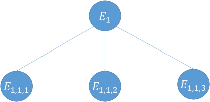
Figure 3: Tree $E_{1}$: both source and destination roads are on two parallel roads and are charging.

(a) Event $E_{1,1,1}$

(b) Event $E_{1,1,2}$

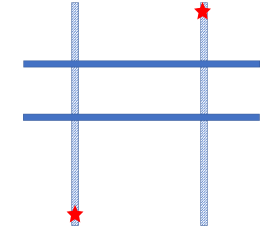
(c) Event $E_{1,1,3}$

(d)

Figure 4: Subcases of tree $E_{1}$.

• Event $E_{1,1,1}$:
  Description: If there are no horizontal roads between S and D, as shown in Fig. 4a;
  Event $L_{1,1}=E_{1,1,1}\cap E_{1}$;
  Probability: $\mathbb{P}(E_{1,1,1}|E_{1})=e^{-\lambda d_{v}}$, $\mathbb{P}(L_{1,1})=\mathbb{P}(E_{1,1,1}|E_{1})\mathbb{P}(E_{1})$;
  Action: we simply use the nearest horizontal road, whether it is below the source or above the destination.

• Event $E_{1,1,2}$:
  Description: If there is at least one horizontal charging road between S and D, as shown in Fig. 4b;
  Event $L_{1,2}=E_{1,1,2}\cap E_{1}$;
  Probability: $\mathbb{P}(E_{1,1,2}|E_{1})=1-e^{-\lambda pd_{v}}$, $\mathbb{P}(L_{1,2})=\mathbb{P}(E_{1,1,2}|E_{1})\mathbb{P}(E_{1})$;
  Action: we can take any horizontal charging road between S and D.

• Event $E_{1,1,3}$:
  Description: If there are no horizontal charging roads but at least one horizontal non-charging road between S and D, as shown in Fig. 4c;
  Event $L_{1,3}=E_{1,1,3}\cap E_{1}$;
  Probability: $\mathbb{P}(E_{1,1,3}|E_{1})=e^{-\lambda pd_{v}}(1-e^{-\lambda(1-p)d_{v}})$, $\mathbb{P}(L_{1,3})=\mathbb{P}(E_{1,1,3}|E_{1})\mathbb{P}(E_{1})$;
  Action: we take any horizontal non-charging road between S and D.

Since the source road is already a charging road, $\mathbb{P}(D_{n}<x|L_{1,i})=1$ for all $i$.

Appendix C proof of Lemma 2

In this appendix, we outline the proof for the probability that the distance to the nearest charging road is less than a positive real number $x$ given the event $E_{2}$, i.e., $\mathbb{P}(D_{n}<x|E_{2})$. As shown in Fig. 5, we hereby denote subevents as $E_{2,i,j}$, in which $i$ is the level of depth of the event in the probability tree and $j$ is the index of the event at that level. Representative figures for $E_{2}$ are shown in Fig. 6. The distribution of $D_{n}$ given $E_{2}$ can be derived as follows:

$$\mathbb{P}(D_{n}<x|E_{2})\mathbb{P}(E_{2})=\sum_{i=1}^{N_{2}}\mathbb{P}(D_{n}<x|L_{2,i})\mathbb{P}(L_{2,i}),$$

where $N_{2}$ denotes the number of leaves of tree $E_{2}$, i.e., $N_{2}=6$, and $L_{2,i}$’s are successive events ending at the leaves of tree $E_{2}$ as shown in Fig. 5. The definition for each event $L_{2,i}$ will be given in more details as we visit each leaf of the tree.

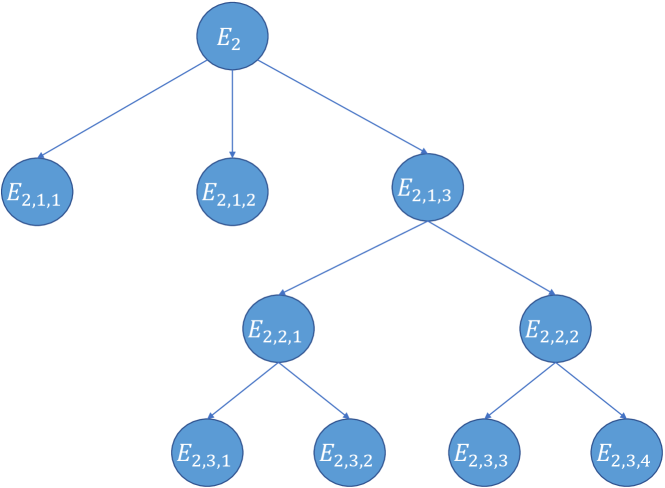
Figure 5: Tree $E_{2}$: both source and destination roads are on two parallel roads and only the source road is charging.

(a) Event $E_{2,1,1}$

(b) Event $E_{2,1,2}$

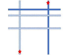
(c) Event $E_{2,3,1}$

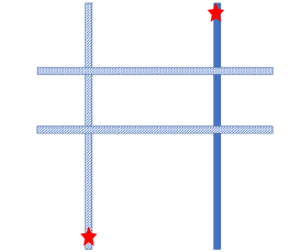
(d) Event $E_{2,3,2}$

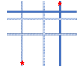
(e) Event $E_{2,3,3}$

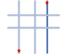
(f) Event $E_{2,3,4}$

(g)

Figure 6: Subcases of tree $E_{2}$.

• Event $E_{2,1,1}$:
  Description: If there are no horizontal roads between S and D, as shown in Fig. 6a;
  Event $L_{2,1}=E_{2,1,1}\cap E_{2}$;
  Probability: $\mathbb{P}(E_{2,1,1}|E_{2})=e^{-\lambda d_{v}}$, $\mathbb{P}(L_{2,1})=\mathbb{P}(E_{2,1,1}|E_{2})\mathbb{P}(E_{2})$;
  Action: we simply take the shortest path from S to D (either upper path or lower path).

• Event $E_{2,1,2}$:
  Description: If there are no horizontal charging roads but at least one horizontal non-charging road between S and D, as shown in Fig. 6b;
  Event $L_{2,2}=E_{2,1,2}\cap E_{2}$;
  Probability: $\mathbb{P}(E_{2,1,2}|E_{2})=e^{-\lambda pd_{v}}(1-e^{-\lambda(1-p)d_{v}})$, $\mathbb{P}(L_{2,2})=\mathbb{P}(E_{2,1,2}|E_{2})\mathbb{P}(E_{2})$;
  Action: we take the furthest horizontal non-charging road from S.

• Event $E_{2,1,3}$:
  Description: If there is at least one horizontal charging road between S and D;
  Probability: $\mathbb{P}(E_{2,1,3}|E_{2})=1-e^{-\lambda pd_{v}}$.

  • Event $E_{2,2,1}$:
    Description: If there are no vertical charging roads between S and D;
    Probability: $\mathbb{P}(E_{2,2,1}|E_{2,1,3},E_{2})=e^{-\lambda pd_{h}}$.

    • Event $E_{2,3,1}$:
      Description: If there exists at least one horizontal non-charging road above the furthest horizontal charging road from S, as shown in Fig. 6c;
      Event $L_{2,3}=E_{2,3,1}\cap E_{2,2,1}\cap E_{2,1,3}\cap E_{2}$;
      Probability: $\mathbb{P}(E_{2,3,1}|E_{2,2,1},E_{2,1,3},E_{2})=1-\frac{p-pe^{-\lambda d_{v}}}{1-e^{-\lambda pd_{v}}}$,
      $\mathbb{P}(L_{2,3})=\mathbb{P}(E_{2,3,1}|E_{2,2,1},E_{2,1,3},E_{2})\times\\ \mathbb{P}(E_{2,2,1}|E_{2,1,3},E_{2})\mathbb{P}(E_{2,1,3}|E_{2})\mathbb{P}(E_{2})$;
      Action: we compare (i) the vertical distance between the furthest horizontal charging road and the furthest horizontal non charging road, and (ii) $d_{h}$, to take the longer one.

    • Event $E_{2,3,2}$:
      Description: If there does not exist horizontal non-charging roads above the furthest horizontal charging road from S, as shown in Fig. 6d;
      Event $L_{2,4}=E_{2,3,2}\cap E_{2,2,1}\cap E_{2,1,3}\cap E_{2}$;
      Probability: $\mathbb{P}(E_{2,3,2}|E_{2,2,1},E_{2,1,3},E_{2})=\frac{p-pe^{-\lambda d_{v}}}{1-e^{-\lambda pd_{v}}}$,
      $\mathbb{P}(L_{2,4})=\mathbb{P}(E_{2,3,2}|E_{2,2,1},E_{2,1,3},E_{2})\times\\ \mathbb{P}(E_{2,2,1}|E_{2,1,3},E_{2})\mathbb{P}(E_{2,1,3}|E_{2})\mathbb{P}(E_{2})$;
      Action: we simply take the furthest horizontal charging road.

  • Event $E_{2,2,2}$:
    Description: If there is at least one vertical charging road between S and D;
    Probability: $\mathbb{P}(E_{2,2,2}|E_{2,1,3},E_{2})=1-e^{-\lambda pd_{h}}$.

    • Event $E_{2,3,3}$:
      Description: If there exists at least one horizontal non-charging road above the furthest horizontal charging road from S, as shown in Fig. 6e;
      Event $L_{2,5}=E_{2,3,3}\cap E_{2,2,2}\cap E_{2,1,3}\cap E_{2}$;
      Probability: $\mathbb{P}(E_{2,3,3}|E_{2,2,2},E_{2,1,3},E_{2})=1-\frac{p-pe^{-\lambda d_{v}}}{1-e^{-\lambda pd_{v}}}$,
      $\mathbb{P}(L_{2,5})=\mathbb{P}(E_{2,3,3}|E_{2,2,2},E_{2,1,3},E_{2})\times\\ \mathbb{P}(E_{2,2,2}|E_{2,1,3},E_{2})\mathbb{P}(E_{2,1,3}|E_{2})\mathbb{P}(E_{2})$;
      Action: we compare (i) the distance between the furthest horizontal charging road and the furthest horizontal non-charging road and (ii) the horizontal distance between the furthest vertical charging road and destination, to take the longer one.

    • Event $E_{2,3,4}$:
      Description: If there does not exist horizontal non-charging roads above the furthest horizontal charging road from S, as shown in Fig. 6f;
      Event $L_{2,6}=E_{2,3,4}\cap E_{2,2,2}\cap E_{2,1,3}\cap E_{2}$;
      Probability: $\mathbb{P}(E_{2,3,4}|E_{2,2,2},E_{2,1,3},E_{2})=\frac{p-pe^{-\lambda d_{v}}}{1-e^{-\lambda pd_{v}}}$,
      $\mathbb{P}(L_{2,6})=\mathbb{P}(E_{2,3,4}|E_{2,2,2},E_{2,1,3},E_{2})\times\\ \mathbb{P}(E_{2,2,2}|E_{2,1,3},E_{2})\mathbb{P}(E_{2,1,3}|E_{2})\mathbb{P}(E_{2})$;
      Action: we simply go with the furthest horizontal charging road.

Since the source road is already a charging road, $\mathbb{P}(D_{n}<x|L_{2,i})=1$ for all $i$.

Appendix D proof of Lemma 3

In this appendix, we first provide a table of functions that are frequently used in later proofs in Table II. Next, the complete form of Lemma 3, i.e., the distribution of $D_{n}$ given $E_{3}$, is given as follows:

$$\mathbb{P}(D_{n}<x|E_{3})\mathbb{P}(E_{3})=\Psi_{1}(p,\lambda,d_{h},d_{v},x)=\sum_{i=1}^{8}C_{i},$$ (15)

where

$$C_{1}=$$

$$\biggl{(}{\textstyle\frac{p(g_{1}+g_{2}+g_{3})\mathbbm{1}\{x>d_{v}\}}{f_{1}(0,\infty,d_{v},t+d_{v},y,d_{v})+f_{1}(0,\infty,t+d_{v},\infty,t+d_{v},d_{v})}}$$

$$+{\textstyle\frac{(1-p)(g_{4}+g_{5}+g_{6})\mathbbm{1}\{x-d_{h}-d_{v}>0\}}{f_{3}(0,\infty,d_{v},t+d_{v},y,d_{v})+f_{3}(0,\infty,t+d_{v},\infty,t+d_{v},d_{v})}}$$

$$+p\frac{f_{2}(d_{v},\infty,0,{\rm min}(x,t-d_{v}),t,y+d_{v})}{f_{2}(d_{v},\infty,0,t-d_{v},t,y+d_{v})}$$

$$+p\frac{f_{4}(d_{v},\infty,0,{\rm min}(x,t-d_{v}),t,y+d_{v})}{f_{4}(d_{v},\infty,0,t-d_{v},t,y+d_{v})}$$

$$+(1-p)\frac{f_{2}(d_{v},\infty,0,{\rm min}(x-d_{h},t-d_{v}),t,y+d_{v})}{f_{2}(d_{v},\infty,0,t-d_{v},t,y+d_{v})}\times$$

$$\mathbbm{1}\{x-d_{h}>0\}$$

$$+(1-p)\times$$

$$\frac{f_{5}(0,x-d_{h},t+d_{v},\infty,y)+f_{5}(0,x-d_{h},d_{v},t+d_{v},t+d_{v})}{f_{5}(0,\infty,t+d_{v},\infty,y)+f_{5}(0,\infty,d_{v},t+d_{v},t+d_{v})}$$

$$\times\mathbbm{1}\{x-d_{h}>0\}\biggr{)}e^{-\lambda d_{v}}\frac{p(1-p)}{2},$$

$$C2=$$

$$\biggl{(}\frac{1-e^{-\lambda(1-p)(x-d_{h})}}{1-e^{-\lambda(1-p)d_{v}}}\mathbbm{1}\{d_{h}<x<d_{h}+d_{v}\}$$

$$+\mathbbm{1}\{d_{h}+d_{v}<x\}\biggr{)}e^{-\lambda pd_{v}}\biggl{(}\lambda(1-p)d_{v}e^{-\lambda(1-p)d_{v}}$$

$$+e^{-\lambda pd_{h}}(1-e^{-\lambda(1-p)d_{v}}-\lambda(1-p)d_{v}e^{-\lambda(1-p)d_{v}})\biggr{)}\times$$

$$\frac{p(1-p)}{2},$$

$$C_{3}=$$

$$\biggl{(}\biggl{(}\frac{\int_{{\rm max}(x-d_{v},0)}^{{\rm min}(d_{h},x)}F_{D_{\mathrm{N-HNC}}}(x-y)f_{D_{\mathrm{N-VC}}}(y){\rm d}y}{F_{D_{\mathrm{N-HNC}}}(d_{v})F_{D_{\mathrm{N-VC}}}(d_{h})}$$

$$+\frac{F_{D_{\mathrm{N-VC}}}({\rm min}(d_{h},x-d_{v}))\mathbbm{1}\{x>d_{v}\}}{F_{D_{\mathrm{N-VC}}}(d_{h})}\biggr{)}\times$$

$$\mathbbm{1}\{x<d_{h}+d_{v}\}+\mathbbm{1}\{x>d_{h}+d_{v}\}\biggr{)}(1-e^{-\lambda pd_{h}})e^{-\lambda pd_{v}}$$

$$\times(1-e^{-\lambda(1-p)d_{v}}-\lambda(1-p)d_{v}e^{-\lambda(1-p)d_{v}})\frac{p(1-p)}{2},$$

$$C_{4}=$$

$$\biggl{(}{\textstyle\frac{f_{6}(0,{\rm max}(x-d_{h},0),d_{h}+y,y)+f_{6}({\rm max}(x-d_{h},0),x,x,y)}{f_{6}(0,{\rm max}(d_{v}-d_{h},0),d_{h}+y,y)+f_{6}({\rm max}(d_{v}-d_{h},0),d_{v},d_{v},y)}}\times$$

$$\mathbbm{1}\{x<d_{v}\}+\mathbbm{1}\{x>d_{v}\}\biggr{)}F_{X_{2}}(d_{h})\biggl{(}1-\frac{p-pe^{-\lambda d_{v}}}{1-e^{-\lambda pd_{v}}}\biggr{)}\times$$

$$e^{-\lambda pd_{h}}(1-e^{-\lambda pd_{v}})\frac{p(1-p)}{2},$$

$$C_{5}=$$

$$\biggl{(}\frac{f_{10}(x,d_{v},x-d_{h})+f_{10}(d_{h},{\rm min}(x,d_{v}),y-d_{h})}{f_{6}(0,d_{v}-d_{h},d_{v},d_{h}+y)}\times$$

$$\mathbbm{1}\{d_{h}<x<d_{v}\}+\mathbbm{1}\{x>d_{v}\}\biggr{)}(1-F_{X_{2}}(d_{h}))\times$$

$$\biggl{(}1-\frac{p-pe^{-\lambda d_{v}}}{1-e^{-\lambda pd_{v}}}\biggr{)}e^{-\lambda pd_{h}}(1-e^{-\lambda pd_{v}})\frac{p(1-p)}{2},$$

$$C_{6}=$$

$$\biggl{(}\frac{f_{7}(x,\infty,x)+f_{7}(0,x,y)}{f_{7}(d_{v},\infty,d_{v})+f_{7}(0,d_{v},y)}\mathbbm{1}\{x<d_{v}\}+\mathbbm{1}\{x>d_{v}\}\biggr{)}$$

$$\times\frac{p-pe^{-\lambda d_{v}}}{1-e^{-\lambda pd_{v}}}(1-e^{-\lambda pd_{v}})\frac{p(1-p)}{2},$$

$$C_{7}=$$

$$\biggl{(}\frac{f_{8}(0,x,x,d_{v},x-t)+f_{8}(0,x,t,x,y-t)}{f_{9}(0,d_{v},0,d_{v}-t,d_{v},t+y)}\mathbbm{1}\{x<d_{v}\}$$

$$+\mathbbm{1}\{x>d_{v}\}\biggr{)}\biggl{(}1-\int_{0}^{d_{h}}F_{X_{2}}(x)f_{D_{\mathrm{N-VC}}}(x){\rm d}x\biggr{)}\times$$

$$\biggl{(}1-\frac{p-pe^{-\lambda d_{v}}}{1-e^{-\lambda pd_{v}}}\biggr{)}(1-e^{-\lambda pd_{h}})(1-e^{-\lambda pd_{v}})\frac{p(1-p)}{2},$$

$$C_{8}=$$

$$\biggl{(}{\textstyle\frac{f_{9}(0,x,0,{\rm max}(x-t,0),y+t,y)+f_{9}(0,\infty,{\rm max}(x-t,0),x,x,y)}{f_{9}(0,\infty,0,{\rm max}(d_{v}-t,0),y+t,y)+f_{9}(0,\infty,{\rm max}(d_{v}-t,0),d_{v},x,y)}}\times$$

$$\mathbbm{1}\{x<d_{v}\}+\mathbbm{1}\{x>d_{v}\}\biggr{)}\int_{0}^{d_{h}}F_{X_{2}}(x)f_{D_{\mathrm{N-VC}}}(x){\rm d}x$$

$$\times\biggl{(}1-\frac{p-pe^{-\lambda d_{v}}}{1-e^{-\lambda pd_{v}}}\biggr{)}(1-e^{-\lambda pd_{h}})(1-e^{-\lambda pd_{v}})\frac{p(1-p)}{2}.$$

Proof:

We prove (15) by further dividing it into subevents, as shown in Fig. 7. We hereby denote subevents as $E_{3,i,j}$, in which $i$ is the level of depth of the event in the probability tree and $j$ is the index of the event at that level. Representative figures for $E_{3}$ are shown in Fig. 8. The distribution of $D_{n}$ given $E_{3}$ can be derived as follows:

$$\mathbb{P}(D_{n}<x|E_{3})\mathbb{P}(E_{3})=\sum_{i=1}^{N_{3}}\mathbb{P}(D_{n}<x|L_{3,i})\mathbb{P}(L_{3,i}),$$

where $N_{3}$ denotes the number of leaves of tree $E_{3}$, i.e., $N_{3}=10$, and $L_{3,i}$’s are successive events ending at the leaves of tree $E_{3}$ as shown in Fig. 7. The definition for each event $L_{3,i}$ will be given in more details as we visit each leaf of the tree.

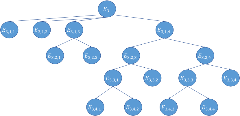
Figure 7: Tree $E_{3}$: both source and destination roads are on two parallel roads and only the destination road is charging.

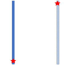
(a) Event $E_{3,1,1}$

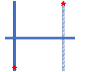
(b) Event $E_{3,1,2}$

(c) Event $E_{3,2,1}$

(d) Event $E_{3,2,2}$

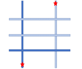
(e) Event $E_{3,3,1}$

(f) Event $E_{3,3,2}$

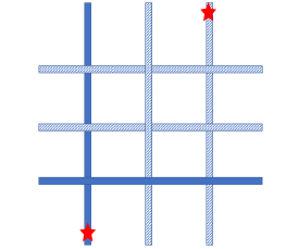
(g) Event $E_{3,3,3}$

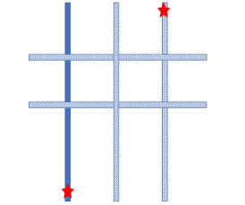
(h) Event $E_{3,3,4}$

(i)

Figure 8: Subcases of tree $E_{3}$.

• Event $E_{3,1,1}$:
  Description: If there are no horizontal roads between S and D, as shown in Fig. 8a;
  Event $L_{3,1}=E_{3,1,1}\cap E_{3}$;
  Probability: $\mathbb{P}(E_{3,1,1}|E_{3})=e^{-\lambda d_{v}}$, $\mathbb{P}(L_{3,1})=\mathbb{P}(E_{3,1,1}|E_{3})\mathbb{P}(E_{3})$;
  Action: we simply take the shortest path from S to D.
  $\mathbb{P}(D_{n}<x|L_{3,1})=\mathbb{P}(D_{n}<x|E_{3,1,1},E_{3})$

  $$=\mathbb{P}(D_{n}<x|D_{\mathrm{N-HC}}>d_{v},D_{\mathrm{N-HNC}}>d_{v})$$

  $$=p\mathbb{P}(D_{\mathrm{N-HC}}<x|D_{\mathrm{N-HC}}<D_{\mathrm{N-HNC}},D_{\mathrm{N-HC}}>d_{v},$$

  $$D_{\mathrm{N-HNC}}>d_{v},D_{\mathrm{N-HC}}<d_{L}+d_{v})$$

  $$+(1-p)\mathbb{P}(D_{\mathrm{N-HNC}}+d_{h}<x|D_{\mathrm{N-HC}}>D_{\mathrm{N-HNC}},$$

  $$D_{\mathrm{N-HC}}>d_{v},D_{\mathrm{N-HNC}}>d_{v},D_{\mathrm{N-HNC}}<d_{L}+d_{v})$$

  $$+p\mathbb{P}(d_{L}<x|D_{\mathrm{N-HC}}>d_{v},D_{\mathrm{N-HNC}}>d_{v},$$

  $$D_{\mathrm{N-HC}}<D_{\mathrm{N-HNC}},d_{L}<D_{\mathrm{N-HC}}-d_{v})$$

  $$+p\mathbb{P}(d_{L}<x|D_{\mathrm{N-HC}}>d_{v},D_{\mathrm{N-HNC}}>d_{v},$$

  $$D_{\mathrm{N-HC}}>D_{\mathrm{N-HNC}},d_{L}<D_{\mathrm{N-HNC}}-d_{v})$$

  $$+(1-p)\mathbb{P}(d_{L}+d_{h}<x|D_{\mathrm{N-HC}}>d_{v},D_{\mathrm{N-HNC}}>d_{v},$$

  $$D_{\mathrm{N-HC}}<D_{\mathrm{N-HNC}},d_{L}<D_{\mathrm{N-HC}}-d_{v})$$

  $$+(1-p)\mathbb{P}(d_{L}+d_{h}<x|D_{\mathrm{N-HC}}>d_{v},D_{\mathrm{N-HNC}}>d_{v},$$

  $$D_{\mathrm{N-HC}}>D_{\mathrm{N-HNC}},d_{L}<D_{\mathrm{N-HNC}}-d_{v})$$

  $$={\textstyle\frac{p(g_{1}+g_{2}+g_{3})}{f_{1}(0,\infty,d_{v},t+d_{v},y,d_{v})+f_{1}(0,\infty,t+d_{v},\infty,t+d_{v},d_{v})}}\times$$

  $$\mathbbm{1}\{x>d_{v}\}$$

  $$+{\textstyle\frac{(1-p)(g_{4}+g_{5}+g_{6})}{f_{3}(0,\infty,d_{v},t+d_{v},y,d_{v})+f_{3}(0,\infty,t+d_{v},\infty,t+d_{v},d_{v})}}\times$$

  $$\mathbbm{1}\{x-d_{h}-d_{v}>0\}$$

  $$+p\frac{f_{2}(d_{v},\infty,0,{\rm min}(x,t-d_{v}),t,y+d_{v})}{f_{2}(d_{v},\infty,0,t-d_{v},t,y+d_{v})}$$

  $$+p\frac{f_{4}(d_{v},\infty,0,{\rm min}(x,t-d_{v}),t,y+d_{v})}{f_{4}(d_{v},\infty,0,t-d_{v},t,y+d_{v})}$$

  $$+(1-p)\frac{f_{2}(d_{v},\infty,0,{\rm min}(x-d_{h},t-d_{v}),t,y+d_{v})}{f_{2}(d_{v},\infty,0,t-d_{v},t,y+d_{v})}\times$$

  $$\mathbbm{1}\{x-d_{h}>0\}$$

  $$+(1-p)\times$$

  $$\frac{f_{5}(0,x-d_{h},t+d_{v},\infty,y)+f_{5}(0,x-d_{h},d_{v},t+d_{v},t+d_{v})}{f_{5}(0,\infty,t+d_{v},\infty,y)+f_{5}(0,\infty,d_{v},t+d_{v},t+d_{v})}$$

  $$\times\mathbbm{1}\{x-d_{h}>0\}$$ (16)

• Event $E_{3,1,2}$:
  Description: If there are no horizontal charging roads but only one horizontal non-charging road between S and D, as shown in Fig. 8b;
  Event $L_{3,2}=E_{3,1,2}\cap E_{3}$;
  Probability: $\mathbb{P}(E_{3,1,2}|E_{3})=e^{-\lambda pd_{v}}\times\\ \lambda(1-p)d_{v}e^{-\lambda(1-p)d_{v}}$, $\mathbb{P}(L_{3,2})=\mathbb{P}(E_{3,1,2}|E_{3})\mathbb{P}(E_{3})$;
  Action: we take the nearest horizontal non-charging road from S.
  $\mathbb{P}(D_{n}<x|L_{3,2})=\mathbb{P}(D_{n}<x|E_{3,1,2},E_{3})$

  $$=\mathbb{P}(D_{\mathrm{N-HNC}}+d_{h}<x|D_{\mathrm{N-HNC}}<d_{v},D_{\mathrm{N-HC}}>d_{v})\times$$

  $$\mathbbm{1}\{d_{h}<x<d_{h}+d_{v}\}+\mathbbm{1}\{x>d_{h}+d_{v}\}$$

  $$=\frac{\mathbb{P}(D_{\mathrm{N-HNC}}<{\rm min}(x-d_{h},d_{v}),D_{\mathrm{N-HC}}>d_{v})}{\mathbb{P}(D_{\mathrm{N-HNC}}<d_{v},D_{\mathrm{N-HC}}>d_{v})}\times$$

  $$\mathbbm{1}\{d_{h}<x<d_{h}+d_{v}\}+\mathbbm{1}\{x>d_{h}+d_{v}\}$$

  $$=\frac{\mathbb{P}(D_{\mathrm{N-HNC}}<x-d_{h})\mathbbm{1}\{d_{h}<x<d_{h}+d_{v}\}}{\mathbb{P}(D_{\mathrm{N-HNC}}<d_{v})\mathbb{P}(D_{\mathrm{N-HC}}>d_{v})}$$

  $$+\frac{\mathbb{P}(D_{\mathrm{N-HNC}}<d_{v})\mathbbm{1}\{x>d_{h}+d_{v}\}\mathbb{P}(D_{\mathrm{N-HC}}>d_{v})}{\mathbb{P}(D_{\mathrm{N-HNC}}<d_{v})\mathbb{P}(D_{\mathrm{N-HC}}>d_{v})}$$

  $$=\frac{F_{D_{\mathrm{N-HNC}}}(x-d_{h})\mathbbm{1}\{d_{h}<x<d_{h}+d_{v}\}}{F_{D_{\mathrm{N-HNC}}}(d_{v})}$$

  $$+\frac{F_{D_{\mathrm{N-HNC}}}(d_{v})\mathbbm{1}\{d_{h}+d_{v}<x\}}{F_{D_{\mathrm{N-HNC}}}(d_{v})}$$

  $$=\frac{1-e^{-\lambda(1-p)(x-d_{h})}}{1-e^{-\lambda(1-p)d_{v}}}\mathbbm{1}\{d_{h}<x<d_{h}+d_{v}\}$$

  $$+\mathbbm{1}\{d_{h}+d_{v}<x\}.$$ (17)

• Event $E_{3,1,3}$:
  Description: If there are no horizontal charging roads but at least two horizontal non-charging road between S and D;
  Probability: $\mathbb{P}(E_{3,1,3}|E_{3})=e^{-\lambda pd_{v}}(1-e^{-\lambda(1-p)d_{v}}-\lambda(1-p)d_{v}e^{-\lambda(1-p)d_{v}})$;

  • Event $E_{3,2,1}$:
    Description: If there are no vertical charging roads between S and D, as shown in Fig. 8c;
    Event $L_{3,3}=E_{3,2,1}\cap E_{3,1,3}\cap E_{3}$;
    Probability: $\mathbb{P}(E_{3,2,1}|E_{3,1,3},E_{3})=e^{-\lambda pd_{h}}$,
    $\mathbb{P}(L_{3,3})=\mathbb{P}(E_{3,2,1}|E_{3,1,3},E_{3})\mathbb{P}(E_{3,1,3}|E_{3})\mathbb{P}(E_{3})$;
    Action: we take the nearest horizontal non-charging road from S.

    $$\mathbb{P}(D_{n}<x|L_{3,3})=\mathbb{P}(D_{n}<x|E_{3,2,1},E_{3,1,3},E_{3})$$

    $$=\frac{1-e^{-\lambda(1-p)(x-d_{h})}}{1-e^{-\lambda(1-p)d_{v}}}\times\mathbbm{1}\{d_{h}<x<d_{h}+d_{v}\}$$

    $$+\mathbbm{1}\{d_{h}+d_{v}<x\}.$$ (18)

    The proof of $\mathbb{P}(D_{n}<x|E_{3,2,1},E_{3,1,3},E_{3})$ is similar to that of $\mathbb{P}(D_{n}<x|E_{3,1,2},E_{3})$ given in (• ‣ D).

  • Event $E_{3,2,2}$:
    Description: If there is at least one vertical charging road between S and D, as shown in Fig. 8d;
    Event $L_{3,4}=E_{3,2,2}\cap E_{3,1,3}\cap E_{3}$;
    Probability: $\mathbb{P}(E_{3,2,2}|E_{3,1,3},E_{3})=1-e^{-\lambda pd_{h}}$,
    $\mathbb{P}(L_{3,4})=\mathbb{P}(E_{3,2,2}|E_{3,1,3},E_{3})\mathbb{P}(E_{3,1,3}|E_{3})\mathbb{P}(E_{3})$;
    Action: we take the nearest horizontal non-charging road from S, then switch to the nearest vertical charging road.
    $\mathbb{P}(D_{n}<x|L_{3,4})=\mathbb{P}(D_{n}<x|E_{3,2,2},E_{3,1,3},E_{3})=$

    $$\mathbb{P}(D_{\mathrm{N-HNC}}+D_{\mathrm{N-VC}}<x|D_{\mathrm{N-HNC}}<d_{v},D_{\mathrm{N-VC}}<d_{h},$$

    $$D_{\mathrm{N-HC}}>d_{v})\mathbbm{1}\{x<d_{h}+d_{v}\}+\mathbbm{1}\{x>d_{h}+d_{v}\}$$

    $$={\textstyle\frac{\mathbb{P}(D_{\mathrm{N-HNC}}+D_{\mathrm{N-VC}}<x,D_{\mathrm{N-HNC}}<d_{v},D_{\mathrm{N-VC}}<d_{h},D_{\mathrm{N-HC}}>d_{v})}{\mathbb{P}(D_{\mathrm{N-HNC}}<d_{v},D_{\mathrm{N-VC}}<d_{h},D_{\mathrm{N-HC}}>d_{v})}}\times$$

    $$\mathbbm{1}\{x<d_{h}+d_{v}\}+\mathbbm{1}\{x>d_{h}+d_{v}\}$$

    $$=\biggl{(}\frac{\int_{{\rm max}(x-d_{v},0)}^{{\rm min}(d_{h},x)}F_{D_{\mathrm{N-HNC}}}(x-y)f_{D_{\mathrm{N-VC}}}(y){\rm d}y}{F_{D_{\mathrm{N-HNC}}}(d_{v})F_{D_{\mathrm{N-VC}}}(d_{h})}$$

    $$+\frac{\int_{0}^{{\rm min}(d_{h},x-d_{v})}F_{D_{\mathrm{N-HNC}}}(d_{v})\mathbbm{1}\{x>d_{v}\}f_{D_{\mathrm{N-VC}}}(r){\rm d}r}{F_{D_{\mathrm{N-HNC}}}(d_{v})F_{D_{\mathrm{N-VC}}}(d_{h})}\biggr{)}\times$$

    $$\mathbbm{1}\{x<d_{h}+d_{v}\}+\mathbbm{1}\{x>d_{h}+d_{v}\}$$

    $$=\biggl{(}\frac{\int_{{\rm max}(x-d_{v},0)}^{{\rm min}(d_{h},x)}F_{D_{\mathrm{N-HNC}}}(x-y)f_{D_{\mathrm{N-VC}}}(y){\rm d}y}{F_{D_{\mathrm{N-HNC}}}(d_{v})F_{D_{\mathrm{N-VC}}}(d_{h})}$$

    $$+\frac{F_{D_{\mathrm{N-VC}}}({\rm min}(d_{h},x-d_{v}))\mathbbm{1}\{x>d_{v}\}}{F_{D_{\mathrm{N-VC}}}(d_{h})}\biggr{)}\times$$

    $$\mathbbm{1}\{x<d_{h}+d_{v}\}+\mathbbm{1}\{x>d_{h}+d_{v}\}.$$ (19)

• Event $E_{3,1,4}$:
  Description: If there is at least one horizontal charging road between S and D;
  Probability: $\mathbb{P}(E_{3,1,4}|E_{3})=1-e^{-\lambda pd_{v}}$.

  • Event $E_{3,2,3}$:
    Description: If there are no vertical charging roads between S and D;
    Probability: $\mathbb{P}(E_{3,2,3}|E_{3,1,4},E_{3})=e^{-\lambda pd_{h}}$.

    • Event $E_{3,3,1}$:
      Description: If there exists at least one horizontal non-charging road below the nearest horizontal charging road from S, as shown in Fig. 8e;
      Probability: $\mathbb{P}(E_{3,3,1}|E_{3,2,3},E_{3,1,4},E_{3})=1-\frac{p-pe^{-\lambda d_{v}}}{1-e^{-\lambda pd_{v}}}$;
      Action: we compare (i) the vertical distance between the nearest horizontal charging road and the nearest horizontal non charging road, and (ii) $d_{h}$, to take the longer one.

      • Event $E_{3,4,1}$:
        Description: If we decide to take the nearest horizontal charging road;
        Event $L_{3,5}=E_{3,4,1}\cap E_{3,3,1}\cap E_{3,2,3}\cap E_{3,1,4}\cap E_{3}$;
        Probability: $\mathbb{P}(E_{3,4,1}|E_{3,3,1},E_{3,2,3},E_{3,1,4},E_{3})=F_{X_{2}}(d_{h})$;
        $\mathbb{P}(L_{3,5})=\mathbb{P}(E_{3,4,1}|E_{3,3,1},E_{3,2,3},E_{3,1,4},E_{3})\times\\ \mathbb{P}(E_{3,3,1}|E_{3,2,3},E_{3,1,4},E_{3})\times\\ \mathbb{P}(E_{3,2,3}|E_{3,1,4},E_{3})\mathbb{P}(E_{3,1,4}|E_{3})\mathbb{P}(E_{3})$;
        $\mathbb{P}(D_{n}<x|L_{3,5})=\mathbb{P}(D_{n}<x|E_{3,4,1},E_{3,3,1},E_{3,2,3},E_{3,1,4},E_{3})=$

        $${\scriptscriptstyle\mathbb{P}(D_{\mathrm{N-HC}}<x|D_{\mathrm{N-HC}}<d_{v},D_{\mathrm{N-HNC}}<D_{\mathrm{N-HC}},D_{\mathrm{N-HNC}}+d_{h}>D_{\mathrm{N-HC}})}\times$$

        $$\mathbbm{1}\{x<d_{v}\}+\mathbbm{1}\{x>d_{v}\}$$

        $$={\textstyle\frac{f_{6}(0,{\rm max}(x-d_{h},0),d_{h}+y,y)+f_{6}({\rm max}(x-d_{h},0),x,x,y)}{f_{6}(0,{\rm max}(d_{v}-d_{h},0),d_{h}+y,y)+f_{6}({\rm max}(d_{v}-d_{h},0),d_{v},d_{v},y)}}\times$$

        $$\mathbbm{1}\{x<d_{v}\}+\mathbbm{1}\{x>d_{v}\}.$$ (20)

      • Event $E_{3,4,2}$:
        Description: If we take the nearest horizontal non-charging road;
        Event $L_{3,6}=E_{3,4,2}\cap E_{3,3,1}\cap E_{3,2,3}\cap E_{3,1,4}\cap E_{3}$;
        Probability: $\mathbb{P}(E_{3,4,2}|E_{3,3,1},E_{3,2,3},E_{3,1,4},E_{3})=1-F_{X_{2}}(d_{h})$;
        $\mathbb{P}(L_{3,6})=\mathbb{P}(E_{3,4,2}|E_{3,3,1},E_{3,2,3},E_{3,1,4},E_{3})\times\\ \mathbb{P}(E_{3,3,1}|E_{3,2,3},E_{3,1,4},E_{3})\times\\ \mathbb{P}(E_{3,2,3}|E_{3,1,4},E_{3})\mathbb{P}(E_{3,1,4}|E_{3})\mathbb{P}(E_{3})$;
        $\mathbb{P}(D_{n}<x|L_{3,6})=\mathbb{P}(D_{n}<x|E_{3,4,2},E_{3,3,1},E_{3,2,3},E_{3,1,4},E_{3})$
        If $d_{h}>d_{v}$, $\mathbb{P}(D_{n}<x|E_{3,4,2},E_{3,3,1},E_{3,2,3},E_{3,1,4},E_{3})=0$.
        If $d_{h}<d_{v}$,

        $$\mathbb{P}(D_{n}<x|E_{3,4,2},E_{3,3,1},E_{3,2,3},E_{3,1,4},E_{3})$$

        $$=\mathbb{P}(D_{\mathrm{N-HNC}}+d_{h}<x|D_{\mathrm{N-HC}}<d_{v},D_{\mathrm{N-HNC}}<D_{\mathrm{N-HC}},$$

        $$d_{h}<D_{\mathrm{N-HC}}-D_{\mathrm{N-HNC}})\mathbbm{1}\{d_{h}<x<d_{v}\}+\mathbbm{1}\{x>d_{v}\}=$$

        $${\scriptstyle\frac{\mathbb{P}(D_{\mathrm{N-HNC}}+d_{h}<x,D_{\mathrm{N-HC}}<d_{v},D_{\mathrm{N-HNC}}<D_{\mathrm{N-HC}},d_{h}<D_{\mathrm{N-HC}}-D_{\mathrm{N-HNC}})}{\mathbb{P}(D_{\mathrm{N-HC}}<d_{v},D_{\mathrm{N-HNC}}<D_{\mathrm{N-HC}},d_{h}<D_{\mathrm{N-HC}}-D_{\mathrm{N-HNC}})}}$$

        $$\times\mathbbm{1}\{d_{h}<x<d_{v}\}+\mathbbm{1}\{x>d_{v}\}$$

        $$=\frac{\mathbb{P}(D_{\mathrm{N-HNC}}+d_{h}<{\rm min}(x,D_{\mathrm{N-HC}}),D_{\mathrm{N-HC}}<d_{v})}{\mathbb{P}(D_{\mathrm{N-HNC}}+d_{h}<D_{\mathrm{N-HC}}<d_{v})}\times$$

        $$\mathbbm{1}\{d_{h}<x<d_{v}\}+\mathbbm{1}\{x>d_{v}\}$$

        $$=\frac{f_{10}(x,d_{v},x-d_{h})+f_{10}(d_{h},{\rm min}(x,d_{v}),y-d_{h})}{f_{6}(0,d_{v}-d_{h},d_{v},d_{h}+y)}\times$$

        $$\mathbbm{1}\{d_{h}<x<d_{v}\}+\mathbbm{1}\{x>d_{v}\}.$$ (21)

    • Event $E_{3,3,2}$:
      Description: If there does not exist horizontal non-charging roads below the nearest horizontal charging road from S, as shown in Fig. 8f;
      Event $L_{3,7}=E_{3,3,2}\cap E_{3,2,3}\cap E_{3,1,4}\cap E_{3}$;
      Probability: $\mathbb{P}(E_{3,3,2}|E_{3,2,3},E_{3,1,4},E_{3})=\frac{p-pe^{-\lambda d_{v}}}{1-e^{-\lambda pd_{v}}}$,
      $\mathbb{P}(L_{3,7})=\mathbb{P}(E_{3,3,2}|E_{3,2,3},E_{3,1,4},E_{3})\times\\ \mathbb{P}(E_{3,2,3}|E_{3,1,4},E_{3})\mathbb{P}(E_{3,1,4}|E_{3})\mathbb{P}(E_{3})$;
      Action: we simply take the nearest horizontal charging road.

      $$\mathbb{P}(D_{n}<x|L_{3,7})=\mathbb{P}(D_{n}<x|E_{3,3,2},E_{3,2,3},E_{3,1,4},E_{3})$$

      $$=\mathbb{P}(D_{\mathrm{N-HC}}<x|D_{\mathrm{N-HC}}<D_{\mathrm{N-HNC}},D_{\mathrm{N-HC}}<d_{v})$$

      $$=\frac{\mathbb{P}(D_{\mathrm{N-HC}}<{\rm min}(x,D_{\mathrm{N-HNC}},d_{v}))}{\mathbb{P}(D_{\mathrm{N-HC}}<{\rm min}(D_{\mathrm{N-HNC}},d_{v}))}\mathbbm{1}\{x<d_{v}\}$$

      $$+\mathbbm{1}\{x>d_{v}\}$$

      $$=\frac{f_{7}(x,\infty,x)+f_{7}(0,x,y)}{f_{7}(d_{v},\infty,d_{v})+f_{7}(0,d_{v},y)}\mathbbm{1}\{x<d_{v}\}+\mathbbm{1}\{x>d_{v}\}.$$ (22)

  • Event $E_{3,2,4}$:
    Description: If there is at least one vertical charging road between S and D;
    Probability: $\mathbb{P}(E_{3,2,4}|E_{3,1,4},E_{3})=1-e^{-\lambda pd_{h}}$.

    • Event $E_{3,3,3}$:
      Description: If there exists at least one horizontal non-charging road below the nearest horizontal charging road from S, as shown in Fig. 8g;
      Probability: $\mathbb{P}(E_{3,3,3}|E_{3,2,4},E_{3,1,4},E_{3})=1-\frac{p-pe^{-\lambda d_{v}}}{1-e^{-\lambda pd_{v}}}$;
      Action: we compare (i) the distance between the nearest horizontal charging road and the nearest horizontal non-charging road, and (ii) the horizontal distance between the nearest vertical charging road and source, to take the longer one.

      • Event $E_{3,4,3}$:
        Description: If we take the nearest vertical charging road;
        Event $L_{3,8}=E_{3,4,3}\cap E_{3,3,3}\cap E_{3,2,4}\cap E_{3,1,4}\cap E_{3}$;
        Probability: $\mathbb{P}(E_{3,4,3}|E_{3,3,3},E_{3,2,4},E_{3,1,4},E_{3})=1-\int_{0}^{d_{h}}F_{X_{2}}(x)f_{D_{\mathrm{N-VC}}}(x){\rm d}x$;
        $\mathbb{P}(L_{3,8})=\mathbb{P}(E_{3,4,3}|E_{3,3,3},E_{3,2,4},E_{3,1,4},E_{3})\times\\ \mathbb{P}(E_{3,3,3}|E_{3,2,4},E_{3,1,4},E_{3})\times\\ \mathbb{P}(E_{3,2,4}|E_{3,1,4},E_{3})\mathbb{P}(E_{3,1,4}|E_{3})\mathbb{P}(E_{3})$;

        $$\mathbb{P}(D_{n}<x|L_{3,8})$$

        $$=\mathbb{P}(D_{n}<x|E_{3,4,3},E_{3,3,3},E_{3,2,4},E_{3,1,4},E_{3})$$

        $$=\mathbb{P}(D_{\mathrm{N-HNC}}+D_{\mathrm{N-VC}}<x|D_{\mathrm{N-HC}}<d_{v},$$

        $$D_{\mathrm{N-HNC}}<D_{\mathrm{N-HC}},D_{\mathrm{N-HC}}>D_{\mathrm{N-VC}}+D_{\mathrm{N-HNC}})\times$$

        $$\mathbbm{1}\{x<d_{v}\}+\mathbbm{1}\{x>d_{v}\}$$

        $$=\frac{\mathbb{P}(D_{\mathrm{N-HNC}}+D_{\mathrm{N-VC}}<{\rm min}(x,D_{\mathrm{N-HC}}),D_{\mathrm{N-HC}}<d_{v})}{\mathbb{P}(D_{\mathrm{N-HNC}}+D_{\mathrm{N-VC}}<D_{\mathrm{N-HC}}<d_{v})}$$

        $$\times\mathbbm{1}\{x<d_{v}\}+\mathbbm{1}\{x>d_{v}\}$$

        $$=\frac{f_{8}(0,x,x,d_{v},x-t)+f_{8}(0,x,t,x,y-t)}{f_{9}(0,d_{v},0,d_{v}-t,d_{v},t+y)}\mathbbm{1}\{x<d_{v}\}+$$

        $$\mathbbm{1}\{x>d_{v}\}.$$ (23)

      • Event $E_{3,4,4}$:
        Description: If we take the nearest horizontal charging road;
        Event $L_{3,9}=E_{3,4,4}\cap E_{3,3,3}\cap E_{3,2,4}\cap E_{3,1,4}\cap E_{3}$;
        Probability: $\mathbb{P}(E_{3,4,4}|E_{3,3,3},E_{3,2,4},E_{3,1,4},E_{3})=\int_{0}^{d_{h}}F_{X_{2}}(x)f_{D_{\mathrm{N-VC}}}(x){\rm d}x$;
        $\mathbb{P}(L_{3,9})=\mathbb{P}(E_{3,4,4}|E_{3,3,3},E_{3,2,4},E_{3,1,4},E_{3})\times\\ \mathbb{P}(E_{3,3,3}|E_{3,2,4},E_{3,1,4},E_{3})\times\\ \mathbb{P}(E_{3,2,4}|E_{3,1,4},E_{3})\mathbb{P}(E_{3,1,4}|E_{3})\mathbb{P}(E_{3})$;

        $$\mathbb{P}(D_{n}<x|L_{3,9})=\mathbb{P}(D_{n}<x|E_{3,4,4},E_{3,3,3},E_{3,2,4},E_{3,1,4},E_{3})$$

        $$=\mathbb{P}(D_{\mathrm{N-HC}}<x|D_{\mathrm{N-HC}}<d_{v},D_{\mathrm{N-HNC}}<D_{\mathrm{N-HC}},$$

        $$D_{\mathrm{N-HC}}-D_{\mathrm{N-HNC}}<D_{\mathrm{N-VC}})$$

        $$=\frac{\mathbb{P}(D_{\mathrm{N-HNC}}<D_{\mathrm{N-HC}}<{\rm min}(x,d_{v},D_{\mathrm{N-HNC}}+D_{\mathrm{N-VC}}))}{\mathbb{P}(D_{\mathrm{N-HNC}}<D_{\mathrm{N-HC}}<{\rm min}(d_{v},D_{\mathrm{N-HNC}}+D_{\mathrm{N-VC}}))}$$

        $$\times\mathbbm{1}\{x<d_{v}\}+\mathbbm{1}\{x>d_{v}\}$$

        $$={\textstyle\frac{f_{9}(0,x,0,{\rm max}(x-t,0),y+t,y)+f_{9}(0,\infty,{\rm max}(x-t,0),x,x,y)}{f_{9}(0,\infty,0,{\rm max}(d_{v}-t,0),y+t,y)+f_{9}(0,\infty,{\rm max}(d_{v}-t,0),d_{v},x,y)}}\times$$

        $$\mathbbm{1}\{x<d_{v}\}+\mathbbm{1}\{x>d_{v}\}.$$ (24)

    • Event $E_{3,3,4}$:
      Description: If there does not exist horizontal non-charging roads below the nearest horizontal charging road from S, as shown in Fig. 8h;
      Event $L_{3,10}=E_{3,3,4}\cap E_{3,2,4}\cap E_{3,1,4}\cap E_{3}$;
      Probability: $\mathbb{P}(E_{3,3,4}|E_{3,2,4},E_{3,1,4},E_{3})=\frac{p-pe^{-\lambda d_{v}}}{1-e^{-\lambda pd_{v}}}$,
      $\mathbb{P}(L_{3,10})=\mathbb{P}(E_{3,3,4}|E_{3,2,4},E_{3,1,4},E_{3})\times\\ \mathbb{P}(E_{3,2,4}|E_{3,1,4},E_{3})\mathbb{P}(E_{3,1,4}|E_{3})\mathbb{P}(E_{3})$;
      Action: we simply take the nearest horizontal charging road.

      $$\mathbb{P}(D_{n}<x|L_{3,10})=\mathbb{P}(D_{n}<x|E_{3,3,4},E_{3,2,4},E_{3,1,4},E_{3})$$

      $$=\mathbb{P}(D_{\mathrm{N-HC}}<x|D_{\mathrm{N-HC}}<D_{\mathrm{N-HNC}},D_{\mathrm{N-HC}}<d_{v})$$

      $$=\frac{\mathbb{P}(D_{\mathrm{N-HC}}<{\rm min}(x,D_{\mathrm{N-HNC}})}{\mathbb{P}(D_{\mathrm{N-HC}}<{\rm min}(D_{\mathrm{N-HNC}},d_{v}))}\mathbbm{1}\{x<d_{v}\}+\mathbbm{1}\{x>d_{v}\}$$

      $$=\frac{f_{7}(0,x,y)+f_{7}(x,\infty,x)}{f_{7}(0,d_{v},y)+f_{7}(d_{v},\infty,d_{v})}\mathbbm{1}\{x<d_{v}\}+\mathbbm{1}\{x>d_{v}\}.$$ (25)

∎

Appendix E proof of Lemma 4

In this appendix, we first provide the complete form of Lemma 4, i.e., the distribution of $D_{n}$ given $E_{4}$, as follows:

$$\mathbb{P}(D_{n}<x|E_{4})\mathbb{P}(E_{4})=\sum_{i=1}^{6}C_{i},$$ (26)

where

$$C_{1}=$$

$$\biggl{(}{\textstyle\frac{p(g_{1}+g_{2}+g_{3})\mathbbm{1}\{x>d_{v}\}}{f_{1}(0,\infty,d_{v},t+d_{v},y,d_{v})+f_{1}(0,\infty,t+d_{v},\infty,t+d_{v},d_{v})}}$$

$$+p\frac{f_{2}(d_{v},\infty,0,{\rm min}(x,t-d_{v}),t,y+d_{v})}{f_{2}(d_{v},\infty,0,t-d_{v},t,y+d_{v})}$$

$$+p\frac{f_{4}(d_{v},\infty,0,{\rm min}(x,t-d_{v}),t,y+d_{v})}{f_{4}(d_{v},\infty,0,t-d_{v},t,y+d_{v})}\biggr{)}e^{-\lambda d_{v}}\frac{(1-p)^{2}}{2},$$

$$C_{2}=$$

$$\biggl{(}\frac{F_{D_{\mathrm{N-HC}}}(x)}{F_{D_{\mathrm{N-HC}}}(d_{v})}\mathbbm{1}\{x<d_{v}\}+\mathbbm{1}\{x>d_{v}\}\biggr{)}\biggl{(}\lambda pd_{v}e^{-\lambda pd_{v}}\times$$

$$e^{-\lambda(1-p)d_{v}}+e^{-\lambda pd_{h}}\lambda pd_{v}e^{-\lambda pd_{v}}(1-e^{-\lambda(1-p)d_{v}})+$$

$$e^{-\lambda pd_{h}}(1-e^{-\lambda pd_{v}}-\lambda pd_{v}e^{-\lambda pd_{v}})\biggr{)}\frac{(1-p)^{2}}{2},$$

$$C_{3}=$$

$$\biggl{(}\biggl{(}\frac{\int_{{\rm max}(x-d_{v},0)}^{{\rm min}(d_{h},x)}F_{D_{\mathrm{N-HNC}}}(x-y)f_{D_{\mathrm{N-VC}}}(y){\rm d}y}{F_{D_{\mathrm{N-HNC}}}(d_{v})F_{D_{\mathrm{N-VC}}}(d_{h})}$$

$$+\frac{F_{D_{\mathrm{N-VC}}}({\rm min}(d_{h},x-d_{v}))\mathbbm{1}\{x>d_{v}\}}{F_{D_{\mathrm{N-VC}}}(d_{h})}\biggr{)}\times$$

$$\mathbbm{1}\{x<d_{h}+d_{v}\}+\mathbbm{1}\{x>d_{h}+d_{v}\}\biggr{)}(1-e^{-\lambda pd_{h}})e^{-\lambda pd_{v}}\times$$

$$(1-e^{-\lambda(1-p)d_{v}}-\lambda(1-p)d_{v}e^{-\lambda(1-p)d_{v}})\frac{(1-p)^{2}}{2},$$

$$C_{4}=$$

$$\biggl{(}\frac{f_{8}(0,x,x,d_{v},x-t)+f_{8}(0,x,t,x,y-t)}{f_{9}(0,d_{v},0,d_{v}-t,d_{v},t+y)}\mathbbm{1}\{x<d_{v}\}$$

$$+\mathbbm{1}\{x>d_{v}\}\biggr{)}\biggl{(}1-\int_{0}^{d_{h}}F_{X_{2}}(x)f_{D_{\mathrm{N-VC}}}(x){\rm d}x\biggr{)}\times$$

$$\biggl{(}1-\frac{p-pe^{-\lambda d_{v}}}{1-e^{-\lambda pd_{v}}}\biggr{)}(1-e^{-\lambda pd_{h}})\biggl{(}\lambda pd_{v}e^{-\lambda pd_{v}}\times$$

$$(1-e^{-\lambda(1-p)d_{v}})+(1-e^{-\lambda pd_{v}}-\lambda pd_{v}e^{-\lambda pd_{v}})\biggr{)}\frac{(1-p)^{2}}{2},$$

$$C_{5}=$$

$$\biggl{(}{\textstyle\frac{f_{9}(0,x,0,{\rm max}(x-t,0),y+t,y)+f_{9}(0,\infty,{\rm max}(x-t,0),x,x,y)}{f_{9}(0,\infty,0,{\rm max}(d_{v}-t,0),y+t,y)+f_{9}(0,\infty,{\rm max}(d_{v}-t,0),d_{v},x,y)}}\times$$

$$\mathbbm{1}\{x<d_{v}\}+\mathbbm{1}\{x>d_{v}\}\biggr{)}\biggl{(}\int_{0}^{d_{h}}F_{X_{2}}(x)f_{D_{\mathrm{N-VC}}}(x){\rm d}x\biggr{)}$$

$$\times\biggl{(}1-\frac{p-pe^{-\lambda d_{v}}}{1-e^{-\lambda pd_{v}}}\biggr{)}(1-e^{-\lambda pd_{h}})\biggl{(}\lambda pd_{v}e^{-\lambda pd_{v}}\times$$

$$(1-e^{-\lambda(1-p)d_{v}})+(1-e^{-\lambda pd_{v}}-\lambda pd_{v}e^{-\lambda pd_{v}})\biggr{)}\frac{(1-p)^{2}}{2},$$

$$C_{6}=$$

$$\biggl{(}\frac{f_{7}(0,x,y)+f_{7}(x,\infty,x)}{f_{7}(0,d_{v},y)+f_{7}(d_{v},\infty,d_{v})}\mathbbm{1}\{x<d_{v}\}+\mathbbm{1}\{x>d_{v}\}\biggr{)}$$

$$\times\frac{p-pe^{-\lambda d_{v}}}{1-e^{-\lambda pd_{v}}}(1-e^{-\lambda pd_{h}})\biggl{(}\lambda pd_{v}e^{-\lambda pd_{v}}(1-e^{-\lambda(1-p)d_{v}})$$

$$+(1-e^{-\lambda pd_{v}}-\lambda pd_{v}e^{-\lambda pd_{v}})\biggr{)}\frac{(1-p)^{2}}{2}.$$

Proof:

We prove (26) by further dividing it into subevents, as shown in Fig. 9, we hereby denote subevents as $E_{4,i,j}$, in which $i$ is the level of depth of the event in the probability tree and $j$ is the index of the event at that level. Representative figures for $E_{4}$ are shown in Fig. 10. The distribution of $D_{n}$ given $E_{4}$ can be derived as follows:

$$\mathbb{P}(D_{n}<x|E_{4})\mathbb{P}(E_{4})=\sum_{i=1}^{N_{4}}\mathbb{P}(D_{n}<x|L_{4,i})\mathbb{P}(L_{4,i}),$$

where $N_{4}$ denotes the number of leaves of tree $E_{4}$, i.e., $N_{4}=13$, and $L_{4,i}$’s are successive events ending at the leaves of tree $E_{4}$ as shown in Fig. 9. The definition for each event $L_{4,i}$ will be given in more details as we visit each leaf of the tree.

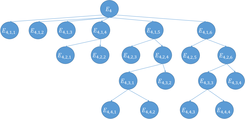
Figure 9: Tree $E_{4}$: both source and destination roads are on two parallel roads and are not charging.

(a) Event $E_{4,1,1}$

(b) Event $E_{4,1,2}$

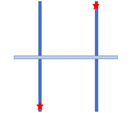
(c) Event $E_{4,1,3}$

(d) Event $E_{4,2,1}$

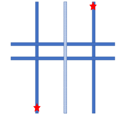
(e) Event $E_{4,2,2}$

(f) Event $E_{4,2,3}$

(g) Event $E_{4,3,1}$

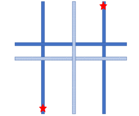
(h) Event $E_{4,3,2}$

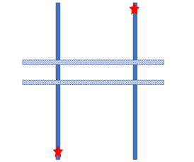
(i) Event $E_{4,2,5}$

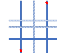
(j) Event $E_{4,3,3}$

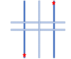
(k) Event $E_{4,3,4}$

(l)

Figure 10: Subcases of tree $E_{4}$.

• Event $E_{4,1,1}$:
  Description: If there are no horizontal roads between S and D, as shown in Fig. 10a;
  Event $L_{4,1}=E_{4,1,1}\cap E_{4}$;
  Probability: $\mathbb{P}(E_{4,1,1}|E_{4})=e^{-\lambda d_{v}}$, $\mathbb{P}(L_{4,1})=\mathbb{P}(E_{4,1,1}|E_{4})\mathbb{P}(E_{4})$;
  Action: We simply take the shortest path from S to D.

  $$\mathbb{P}(D_{n}<x|L_{4,1})=\mathbb{P}(D_{n}<x|E_{4,1,1},E_{4})$$

  $$=\mathbb{P}(D_{n}<x|D_{\mathrm{N-HC}}>d_{v},D_{\mathrm{N-HNC}}>d_{v})$$

  $$={\textstyle\frac{p(g_{1}+g_{2}+g_{3})}{f_{1}(0,\infty,d_{v},t+d_{v},y,d_{v})+f_{1}(0,\infty,t+d_{v},\infty,t+d_{v},d_{v})}}\times$$

  $$\mathbbm{1}\{x>d_{v}\}$$

  $$+p\frac{f_{2}(d_{v},\infty,0,{\rm min}(x,t-d_{v}),t,y+d_{v})}{f_{2}(d_{v},\infty,0,t-d_{v},t,y+d_{v})}$$

  $$+p\frac{f_{4}(d_{v},\infty,0,{\rm min}(x,t-d_{v}),t,y+d_{v})}{f_{4}(d_{v},\infty,0,t-d_{v},t,y+d_{v})}.$$ (27)

  The proof for $\mathbb{P}(D_{n}<x|E_{4,1,1},E_{4})$ is similar to that of $\mathbb{P}(D_{n}<x|E_{3,1,1},E_{3})$ given in (• ‣ D).

• Event $E_{4,1,2}$:
  Description: If there is only one horizontal non-charging road and no horizontal charging road between S and D, as shown in Fig. 10b;
  Event $L_{4,2}=E_{4,1,2}\cap E_{4}$;
  Probability: $\mathbb{P}(E_{4,1,2}|E_{4})=\lambda(1-p)d_{v}e^{-\lambda(1-p)d_{v}}e^{-\lambda pd_{v}}$, $\mathbb{P}(L_{4,2})=\mathbb{P}(E_{4,1,2}|E_{4})\mathbb{P}(E_{4})$;
  Action: We take that horizontal non-charging road.

  $$\mathbb{P}(D_{n}<x|L_{4,2})=\mathbb{P}(D_{n}<x|E_{4,1,2},E_{4})=0$$

• Event $E_{4,1,3}$:
  Description: If there is only one horizontal charging road and no horizontal non-charging road between S and D, as shown in Fig. 10c;
  Event $L_{4,3}=E_{4,1,3}\cap E_{4}$;
  Probability: $\mathbb{P}(E_{4,1,3}|E_{4})=\lambda pd_{v}e^{-\lambda pd_{v}}e^{-\lambda(1-p)d_{v}}$, $\mathbb{P}(L_{4,3})=\mathbb{P}(E_{4,1,3}|E_{4})\mathbb{P}(E_{4})$;
  Action: We take that horizontal charging road.

  $$\mathbb{P}(D_{n}<x|L_{4,3})=\mathbb{P}(D_{n}<x|E_{4,1,3},E_{4})$$

  $$=\mathbb{P}(D_{n}<x|D_{\mathrm{N-HC}}<d_{v},D_{\mathrm{N-HNC}}>d_{v})\mathbbm{1}\{x<d_{v}\}$$

  $$+\mathbbm{1}\{x>d_{v}\}$$

  $$=\frac{\mathbb{P}(D_{\mathrm{N-HC}}<{\rm min}(x,d_{v}),D_{\mathrm{N-HNC}}>d_{v})}{\mathbb{P}(D_{\mathrm{N-HC}}<d_{v}<D_{\mathrm{N-HNC}})}\mathbbm{1}\{x<d_{v}\}$$

  $$+\mathbbm{1}\{x>d_{v}\}$$

  $$=\frac{F_{D_{\mathrm{N-HC}}}(x)}{F_{D_{\mathrm{N-HC}}}(d_{v})}\mathbbm{1}\{x<d_{v}\}+\mathbbm{1}\{x>d_{v}\}.$$ (28)

• Event $E_{4,1,4}$:
  Description: If there are no horizontal charging roads but at least two horizontal non-charging road between S and D;
  Probability: $\mathbb{P}(E_{4,1,4}|E_{4})=e^{-\lambda pd_{v}}(1-e^{-\lambda(1-p)d_{v}}-\lambda(1-p)d_{v}e^{-\lambda(1-p)d_{v}})$.

  • Event $E_{4,2,1}$:
    Description: If there are no vertical charging roads between S and D, as shown in Fig. 10d;
    Event $L_{4,4}=E_{4,2,1}\cap E_{4,1,4}\cap E_{4}$;
    Probability: $\mathbb{P}(E_{4,2,1}|E_{4,1,4},E_{4})=e^{-\lambda pd_{h}}$, $\mathbb{P}(L_{4,4})=\mathbb{P}(E_{4,2,1}|E_{4,1,4},E_{4})\mathbb{P}(E_{4,1,4}|E_{4})\mathbb{P}(E_{4})$;
    Action: We take any horizontal non-charging road between S and D.

    $$\mathbb{P}(D_{n}<x|L_{4,4})=\mathbb{P}(D_{n}<x|E_{4,2,1},E_{4,1,4},E_{4})=0$$

  • Event $E_{4,2,2}$:
    Description: If there is at least one vertical charging road between S and D, as shown in Fig. 10e;
    Event $L_{4,5}=E_{4,2,2}\cap E_{4,1,4}\cap E_{4}$;
    Probability: $\mathbb{P}(E_{4,2,2}|E_{4,1,4},E_{4})=1-e^{-\lambda pd_{h}}$,
    $\mathbb{P}(L_{4,5})=\mathbb{P}(E_{4,2,2}|E_{4,1,4},E_{4})\mathbb{P}(E_{4,1,4}|E_{4})\mathbb{P}(E_{4})$;
    Action: We first go to the nearest horizontal non-charging road, then switch to the nearest vertical charging road, then switch to the furthest horizontal non-charging road.

    $$\mathbb{P}(D_{n}<x|L_{4,5})=\mathbb{P}(D_{n}<x|E_{4,2,2},E_{4,1,4},E_{4})$$

    $$=\biggl{(}\frac{\int_{{\rm max}(x-d_{v},0)}^{{\rm min}(d_{h},x)}F_{D_{\mathrm{N-HNC}}}(x-y)f_{D_{\mathrm{N-VC}}}(y){\rm d}y}{F_{D_{\mathrm{N-HNC}}}(d_{v})F_{D_{\mathrm{N-VC}}}(d_{h})}$$

    $$+\frac{F_{D_{\mathrm{N-VC}}}({\rm min}(d_{h},x-d_{v}))\mathbbm{1}\{x>d_{v}\}}{F_{D_{\mathrm{N-VC}}}(d_{h})}\biggr{)}\times$$

    $$\mathbbm{1}\{x<d_{h}+d_{v}\}+\mathbbm{1}\{x>d_{h}+d_{v}\}.$$ (29)

    The proof for $\mathbb{P}(D_{n}<x|E_{4,2,2},E_{4,1,4},E_{4})$ is similar to that of $\mathbb{P}(D_{n}<x|E_{3,2,2},E_{3,1,3},E_{3})$ given in (– ‣ • ‣ D).

• Event $E_{4,1,5}$:
  Description: If there is one horizontal charging road and at least one horizontal non-charging road between S and D;
  Probability: $\mathbb{P}(E_{4,1,5}|E_{4})=\lambda pd_{v}e^{-\lambda pd_{v}}(1-e^{-\lambda(1-p)d_{v}})$.

  • Event $E_{4,2,3}$:
    Description: If there are no vertical charging roads between S and D, as shown in Fig. 10f;
    Event $L_{4,6}=E_{4,2,3}\cap E_{4,1,5}\cap E_{4}$;
    Probability: $\mathbb{P}(E_{4,2,3}|E_{4,1,5},E_{4})=e^{-\lambda pd_{h}}$, $\mathbb{P}(L_{4,6})=\mathbb{P}(E_{4,2,3}|E_{4,1,5},E_{4})\mathbb{P}(E_{4,1,5}|E_{4})\mathbb{P}(E_{4})$;
    Action: We take the horizontal charging road between S and D.

    $$\mathbb{P}(D_{n}<x|L_{4,6})=\mathbb{P}(D_{n}<x|E_{4,2,3},E_{4,1,5},E_{4})$$

    $$=\mathbb{P}(D_{n}<x|D_{\mathrm{N-HC}}<d_{v},D_{\mathrm{N-HNC}}<d_{v})\mathbbm{1}\{x<d_{v}\}$$

    $$+\mathbbm{1}\{x>d_{v}\}$$

    $$=\frac{F_{D_{\mathrm{N-HC}}}(x)}{F_{D_{\mathrm{N-HC}}}(d_{v})}\mathbbm{1}\{x<d_{v}\}+\mathbbm{1}\{x>d_{v}\}.$$ (30)

    The proof of $\mathbb{P}(D_{n}<x|E_{4,2,3},E_{4,1,5},E_{4})$ is similar to that of $\mathbb{P}(D_{n}<x|E_{4,1,3},E_{4})$ given in (• ‣ E).

  • Event $E_{4,2,4}$:
    Description: If there is at least one vertical charging road between S and D;
    Probability: $\mathbb{P}(E_{4,2,4}|E_{4,1,5},E_{4})=1-e^{-\lambda pd_{h}}$.

    • Event $E_{4,3,1}$:
      Description: If there exists at least one horizontal non-charging road below the nearest horizontal charging road from S, as shown in Fig. 10g;
      Probability: $\mathbb{P}(E_{4,3,1}|E_{4,2,4},E_{4,1,5},E_{4})=1-\frac{p-pe^{-\lambda d_{v}}}{1-e^{-\lambda pd_{v}}}$;
      Action: we compare (i) the distance between the nearest horizontal charging road and the nearest horizontal non-charging road, and (ii) the horizontal distance between the nearest vertical charging road and source, to take the longer one.

      • Event $E_{4,4,1}$:
        Description: If we take the nearest vertical charging road;
        Event $L_{4,7}=E_{4,4,1}\cap E_{4,3,1}\cap E_{4,2,4}\cap E_{4,1,5}\cap E_{4}$;
        Probability: $\mathbb{P}(E_{4,4,1}|E_{4,3,1},E_{4,2,4},E_{4,1,5},E_{4})=1-\int_{0}^{d_{h}}F_{X_{2}}(x)f_{D_{\mathrm{N-VC}}}(x){\rm d}x$;
        $\mathbb{P}(L_{4,7})=\mathbb{P}(E_{4,4,1}|E_{4,3,1},E_{4,2,4},E_{4,1,5},E_{4})\times\\ \mathbb{P}(E_{4,3,1}|E_{4,2,4},E_{4,1,5},E_{4})\times\\ \mathbb{P}(E_{4,2,4}|E_{4,1,5},E_{4})\mathbb{P}(E_{4,1,5}|E_{4})\mathbb{P}(E_{4})$;

        $$\mathbb{P}(D_{n}<x|L_{4,7})=\mathbb{P}(D_{n}<x|E_{4,4,1},E_{4,3,1},E_{4,2,4},E_{4,1,5},E_{4})$$

        $$=\frac{f_{8}(0,x,x,d_{v},x-t)+f_{8}(0,x,t,x,y-t)}{f_{9}(0,d_{v},0,d_{v}-t,d_{v},t+y)}\mathbbm{1}\{x<d_{v}\}$$

        $$+\mathbbm{1}\{x>d_{v}\}.$$ (31)

        The proof of $\mathbb{P}(D_{n}<x|E_{4,4,1},E_{4,3,1},E_{4,2,4},E_{4,1,5},E_{4})$ is similar to that of
        $\mathbb{P}(D_{n}<x|E_{3,4,3},E_{3,3,3},E_{3,2,4},E_{3,1,4},E_{3})$ given in (· ‣ * ‣ – ‣ • ‣ D).

      • Event $E_{4,4,2}$:
        Description: If we take the nearest horizontal charging road;
        Event $L_{4,8}=E_{4,4,2}\cap E_{4,3,1}\cap E_{4,2,4}\cap E_{4,1,5}\cap E_{4}$;
        Probability: $\mathbb{P}(E_{4,4,2}|E_{4,3,1},E_{4,2,4},E_{4,1,5},E_{4})=\int_{0}^{d_{h}}F_{X_{2}}(x)f_{D_{\mathrm{N-VC}}}(x){\rm d}x$;
        $\mathbb{P}(L_{4,8})=\mathbb{P}(E_{4,4,2}|E_{4,3,1},E_{4,2,4},E_{4,1,5},E_{4})\times\\ \mathbb{P}(E_{4,3,1}|E_{4,2,4},E_{4,1,5},E_{4})\times\\ \mathbb{P}(E_{4,2,4}|E_{4,1,5},E_{4})\mathbb{P}(E_{4,1,5}|E_{4})\mathbb{P}(E_{4})$;

        $$\mathbb{P}(D_{n}<x|L_{4,8})=\mathbb{P}(D_{n}<x|E_{4,4,2},E_{4,3,1},E_{4,2,4},E_{4,1,5},E_{4})$$

        $$={\textstyle\frac{f_{9}(0,x,0,{\rm max}(x-t,0),y+t,y)+f_{9}(0,\infty,{\rm max}(x-t,0),x,x,y)}{f_{9}(0,\infty,0,{\rm max}(d_{v}-t,0),y+t,y)+f_{9}(0,\infty,{\rm max}(d_{v}-t,0),d_{v},x,y)}}\times$$

        $$\mathbbm{1}\{x<d_{v}\}+\mathbbm{1}\{x>d_{v}\}.$$ (32)

        The proof of $\mathbb{P}(D_{n}<x|E_{4,4,2},E_{4,3,1},E_{4,2,4},E_{4,1,5},E_{4})$ is similar to that of
        $\mathbb{P}(D_{n}<x|E_{3,4,4},E_{3,3,3},E_{3,2,4},E_{3,1,4},E_{3})$ given in (· ‣ * ‣ – ‣ • ‣ D).

    • Event $E_{4,3,2}$:
      Description: If there does not exist horizontal non-charging roads below the nearest horizontal charging road from S, as shown in Fig. 10h;
      Event $L_{4,9}=E_{4,3,2}\cap E_{4,2,4}\cap E_{4,1,5}\cap E_{4}$;
      Probability: $\mathbb{P}(E_{4,3,2}|E_{4,2,4},E_{4,1,5},E_{4})=\frac{p-pe^{-\lambda d_{v}}}{1-e^{-\lambda pd_{v}}}$,
      $\mathbb{P}(L_{4,9})=\mathbb{P}(E_{4,3,2}|E_{4,2,4},E_{4,1,5},E_{4})\times\\ \mathbb{P}(E_{4,2,4}|E_{4,1,5},E_{4})\mathbb{P}(E_{4,1,5}|E_{4})\mathbb{P}(E_{4})$;
      Action: we simply take the nearest horizontal charging road.

      $$\mathbb{P}(L_{4,9})=\mathbb{P}(D_{n}<x|E_{4,3,2},E_{4,2,4},E_{4,1,5},E_{4})$$

      $$=\frac{f_{7}(0,x,y)+f_{7}(x,\infty,x)}{f_{7}(0,d_{v},y)+f_{7}(d_{v},\infty,d_{v})}\mathbbm{1}\{x<d_{v}\}+\mathbbm{1}\{x>d_{v}\}.$$ (33)

      The proof of $\mathbb{P}(D_{n}<x|E_{4,3,2},E_{4,2,4},E_{4,1,5},E_{4})$ is similar to that of $\mathbb{P}(D_{n}<x|E_{3,3,4},E_{3,2,4},E_{3,1,4},E_{3})$ given in (* ‣ – ‣ • ‣ D).

• Event $E_{4,1,6}$:
  Description: If there are at least two horizontal charging roads between S and D;
  Probability: $\mathbb{P}(E_{4,1,6}|E_{4})=1-e^{-\lambda pd_{v}}-\lambda pd_{v}e^{-\lambda pd_{v}}$.

  • Event $E_{4,2,5}$:
    Description: If there are no vertical charging roads between S and D, as shown in Fig. 10i;
    Event $L_{4,10}=E_{4,2,5}\cap E_{4,1,6}\cap E_{4}$;
    Probability: $\mathbb{P}(E_{4,2,5}|E_{4,1,6},E_{4})=e^{-\lambda pd_{h}}$,
    $\mathbb{P}(L_{4,10})=\mathbb{P}(E_{4,2,5}|E_{4,1,6},E_{4})\mathbb{P}(E_{4,1,6}|E_{4})\mathbb{P}(E_{4})$;
    Action: We take any horizontal charging road between S and D.

    $$\mathbb{P}(D_{n}<x|L_{4,10})=\mathbb{P}(D_{n}<x|E_{4,2,5},E_{4,1,6},E_{4})$$

    $$=\frac{F_{D_{\mathrm{N-HC}}}(x)}{F_{D_{\mathrm{N-HC}}}(d_{v})}\mathbbm{1}\{x<d_{v}\}+\mathbbm{1}\{x>d_{v}\}.$$ (34)

    The proof of $\mathbb{P}(D_{n}<x|E_{4,2,5},E_{4,1,6},E_{4})$ is similar to that of $\mathbb{P}(D_{n}<x|E_{4,1,3},E_{4})$ given in (• ‣ E).

  • Event $E_{4,2,6}$:
    Description: If there is at least one vertical charging road between S and D;
    Probability: $\mathbb{P}(E_{4,2,6}|E_{4,1,6},E_{4})=1-e^{-\lambda pd_{h}}$.

    • Event $E_{4,3,3}$:
      Description: If there exists at least one horizontal non-charging road below the nearest horizontal charging road from S, as shown in Fig. 10j;
      Probability: $\mathbb{P}(E_{4,3,3}|E_{4,2,6},E_{4,1,6},E_{4})=1-\frac{p-pe^{-\lambda d_{v}}}{1-e^{-\lambda pd_{v}}}$;
      Action: we compare (i) the distance between the nearest horizontal charging road and the nearest horizontal non-charging road, and (ii) the horizontal distance between the nearest vertical charging road and source, to take the longer one.

      • Event $E_{4,4,3}$:
        Description: If we take the nearest vertical charging road;
        Event $L_{4,11}=E_{4,4,3}\cap E_{4,3,3}\cap E_{4,2,6}\cap E_{4,1,6}\cap E_{4}$;
        Probability: $\mathbb{P}(E_{4,4,3}|E_{4,3,3},E_{4,2,6},E_{4,1,6},E_{4})=1-\int_{0}^{d_{h}}F_{X_{2}}(x)f_{D_{\mathrm{N-VC}}}(x){\rm d}x$;
        $\mathbb{P}(L_{4,11})=\mathbb{P}(E_{4,4,3}|E_{4,3,3},E_{4,2,6},E_{4,1,6},E_{4})\times\\ \mathbb{P}(E_{4,3,3}|E_{4,2,6},E_{4,1,6},E_{4})\times\\ \mathbb{P}(E_{4,2,6}|E_{4,1,6},E_{4})\mathbb{P}(E_{4,1,6}|E_{4})\mathbb{P}(E_{4})$;

        $$\mathbb{P}(D_{n}<x|L_{4,11})=\mathbb{P}(D_{n}<x|E_{4,4,3},E_{4,3,3},E_{4,2,6},E_{4,1,6},E_{4})$$

        $$=\frac{f_{8}(0,x,x,d_{v},x-t)+f_{8}(0,x,t,x,y-t)}{f_{9}(0,d_{v},0,d_{v}-t,d_{v},t+y)}\mathbbm{1}\{x<d_{v}\}$$

        $$+\mathbbm{1}\{x>d_{v}\}.$$ (35)

        The proof of $\mathbb{P}(D_{n}<x|E_{4,4,3},E_{4,3,3},E_{4,2,6},E_{4,1,6},E_{4})$ is similar to that of
        $\mathbb{P}(D_{n}<x|E_{3,4,3},E_{3,3,3},E_{3,2,4},E_{3,1,4},E_{3})$ given in (· ‣ * ‣ – ‣ • ‣ D).

      • Event $E_{4,4,4}$:
        Description: If we take the nearest horizontal charging road;
        Event $L_{4,12}=E_{4,4,4}\cap E_{4,3,3}\cap E_{4,2,6}\cap E_{4,1,6}\cap E_{4}$;
        Probability: $\mathbb{P}(E_{4,4,4}|E_{4,3,3},E_{4,2,6},E_{4,1,6},E_{4})=\int_{0}^{d_{h}}F_{X_{2}}(x)f_{D_{\mathrm{N-VC}}}(x){\rm d}x$;
        $\mathbb{P}(L_{4,12})=\mathbb{P}(E_{4,4,4}|E_{4,3,3},E_{4,2,6},E_{4,1,6},E_{4})\times\\ \mathbb{P}(E_{4,3,3}|E_{4,2,6},E_{4,1,6},E_{4})\times\\ \mathbb{P}(E_{4,2,6}|E_{4,1,6},E_{4})\mathbb{P}(E_{4,1,6}|E_{4})\mathbb{P}(E_{4})$;

        $$\mathbb{P}(D_{n}<x|L_{4,12})=\mathbb{P}(D_{n}<x|E_{4,4,4},E_{4,3,3},E_{4,2,6},E_{4,1,6},E_{4})$$

        $$={\textstyle\frac{f_{9}(0,x,0,{\rm max}(x-t,0),y+t,y)+f_{9}(0,\infty,{\rm max}(x-t,0),x,x,y)}{f_{9}(0,\infty,0,{\rm max}(d_{v}-t,0),y+t,y)+f_{9}(0,\infty,{\rm max}(d_{v}-t,0),d_{v},x,y)}}\times$$

        $$\mathbbm{1}\{x<d_{v}\}+\mathbbm{1}\{x>d_{v}\}.$$ (36)

        The proof of $\mathbb{P}(D_{n}<x|E_{4,4,4},E_{4,3,3},E_{4,2,6},E_{4,1,6},E_{4})$ is similar to that of
        $\mathbb{P}(D_{n}<x|E_{3,4,4},E_{3,3,3},E_{3,2,4},E_{3,1,4},E_{3})$ given in (· ‣ * ‣ – ‣ • ‣ D).

    • Event $E_{4,3,4}$:
      Description: If there does not exist horizontal non-charging roads below the nearest horizontal charging road from S, as shown in Fig. 10k;
      Event $L_{4,13}=E_{4,3,4}\cap E_{4,2,6}\cap E_{4,1,6}\cap E_{4}$;
      Probability: $\mathbb{P}(E_{4,3,4}|E_{4,2,6},E_{4,1,6},E_{4})=\frac{p-pe^{-\lambda d_{v}}}{1-e^{-\lambda pd_{v}}}$,
      $\mathbb{P}(L_{4,13})=\mathbb{P}(E_{4,3,4}|E_{4,2,6},E_{4,1,6},E_{4})\times\\ \mathbb{P}(E_{4,2,6}|E_{4,1,6},E_{4})\mathbb{P}(E_{4,1,6}|E_{4})\mathbb{P}(E_{4})$;
      Action: we simply take the nearest horizontal charging road.

      $$\mathbb{P}(D_{n}<x|L_{4,13})=\mathbb{P}(D_{n}<x|E_{4,3,4},E_{4,2,6},E_{4,1,6},E_{4})$$

      $$=\frac{f_{7}(0,x,y)+f_{7}(x,\infty,x)}{f_{7}(0,d_{v},y)+f_{7}(d_{v},\infty,d_{v})}\mathbbm{1}\{x<d_{v}\}+\mathbbm{1}\{x>d_{v}\}.$$ (37)

      The proof of $\mathbb{P}(D_{n}<x|E_{4,3,4},E_{4,2,6},E_{4,1,6},E_{4})$ is similar to that of $\mathbb{P}(D_{n}<x|E_{3,3,4},E_{3,2,4},E_{3,1,4},E_{3})$ given in (* ‣ – ‣ • ‣ D).

∎

Appendix F proof of Lemma 6

In this appendix, we outline the proof for the probability that the distance to the nearest charging road is less than a positive real number $x$ given the event $E_{6}$, i.e., $\mathbb{P}(D_{n}<x|E_{6})$. As shown in Fig. 11, we hereby denote subevents as $E_{6,i,j}$, in which $i$ is the level of depth of the event in the probability tree and $j$ is the index of the event at that level. Representative figures for $E_{6}$ are shown in Fig. 12. The distribution of $D_{n}$ given $E_{6}$ can be derived as follows:

$$\mathbb{P}(D_{n}<x|E_{6})\mathbb{P}(E_{6})=\sum_{i=1}^{N_{6}}\mathbb{P}(D_{n}<x|L_{6,i})\mathbb{P}(L_{6,i}),$$

where $N_{6}$ denotes the number of leaves of tree $E_{6}$, i.e., $N_{6}=6$, and $L_{6,i}$’s are successive events ending at the leaves of tree $E_{6}$ as shown in Fig. 11. The definition for each event $L_{6,i}$ will be given in more details as we visit each leaf of the tree.

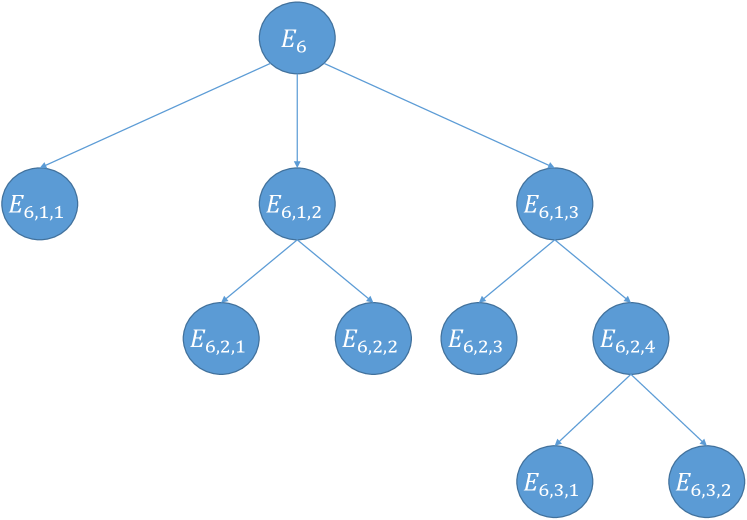
Figure 11: Tree $E_{6}$: source and destination roads are on two perpendicular roads and only the source road is charging.

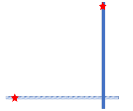
(a) Event $E_{6,1,1}$

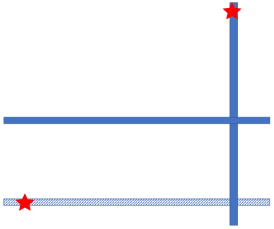
(b) Event $E_{6,2,1}$

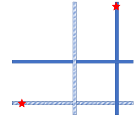
(c) Event $E_{6,2,2}$

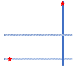
(d) Event $E_{6,2,3}$

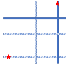
(e) Event $E_{6,3,1}$

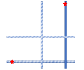
(f) Event $E_{6,3,2}$

(g)

Figure 12: Subcases of tree $E_{6}$.

• Event $E_{6,1,1}$:
  Description: If there are no horizontal roads between S and D, as shown in Fig. 12a;
  Event $L_{6,1}=E_{6,1,1}\cap E_{6}$;
  Probability: $\mathbb{P}(E_{6,1,1}|E_{6})=e^{-\lambda d_{v}}$, $\mathbb{P}(L_{6,1})=\mathbb{P}(E_{6,1,1}|E_{6})\mathbb{P}(E_{6})$;
  Action: We simply take the source road then the destination road.

• Event $E_{6,1,2}$:
  Description: If there are no horizontal charging roads but at least one horizontal non-charging road between S and D;
  Probability: $\mathbb{P}(E_{6,1,2}|E_{6})=e^{-\lambda pd_{v}}(1-e^{-\lambda(1-p)d_{v}})$.

  • Event $E_{6,2,1}$:
    Description: If there are no vertical charging roads between S and D, as shown in Fig. 12b;
    Event $L_{6,2}=E_{6,2,1}\cap E_{6,1,2}\cap E_{6}$;
    Probability: $\mathbb{P}(E_{6,2,1}|E_{6,1,2},E_{6})=e^{-\lambda pd_{h}}$,
    $\mathbb{P}(L_{6,2})=\mathbb{P}(E_{6,2,1}|E_{6,1,2},E_{6})\mathbb{P}(E_{6,1,2}|E_{6})\mathbb{P}(E_{6})$;
    Action: We take the source road then the destination road.

  • Event $E_{6,2,2}$:
    Description: If there is at least one vertical charging road between S and D, as shown in Fig. 12c;
    Event $L_{6,3}=E_{6,2,2}\cap E_{6,1,2}\cap E_{6}$;
    Probability: $\mathbb{P}(E_{6,2,2}|E_{6,1,2},E_{6})=1-e^{-\lambda pd_{h}}$,
    $\mathbb{P}(L_{6,3})=\mathbb{P}(E_{6,2,2}|E_{6,1,2},E_{6})\mathbb{P}(E_{6,1,2}|E_{6})\mathbb{P}(E_{6})$;
    Action: we compare (i) the distance between source and the furthest horizontal non-charging road and (ii) the distance between the furthest vertical charging road to destination, to take the longer one.

• Event $E_{6,1,3}$:
  Description: If there is at least one horizontal charging road between S and D;
  Probability: $\mathbb{P}(E_{6,1,3}|E_{6})=1-e^{-\lambda pd_{v}}$.

  • Event $E_{6,2,3}$:
    Description: If there are no vertical charging roads between S and D, as shown in Fig. 12d;
    Event $L_{6,4}=E_{6,2,3}\cap E_{6,1,3}\cap E_{6}$;
    Probability: $\mathbb{P}(E_{6,2,3}|E_{6,1,3},E_{6})=e^{-\lambda pd_{h}}$,
    $\mathbb{P}(L_{6,4})=\mathbb{P}(E_{6,2,3}|E_{6,1,3},E_{6})\mathbb{P}(E_{6,1,3}|E_{6})\mathbb{P}(E_{6})$;
    Action: We take the source road then the destination road.

  • Event $E_{6,2,4}$:
    Description: If there is at least one vertical charging road between S and D;
    Probability: $\mathbb{P}(E_{6,2,4}|E_{6,1,3},E_{6})=1-e^{-\lambda pd_{h}}$.

    • Event $E_{6,3,1}$:
      Description: If there exists at least one horizontal non-charging road above the furthest horizontal charging road from S, as shown in Fig. 12e;
      Event $L_{6,5}=E_{6,3,1}\cap E_{6,2,4}\cap E_{6,1,3}\cap E_{6}$;
      Probability: $\mathbb{P}(E_{6,3,1}|E_{6,2,4},E_{6,1,3},E_{6})=1-\frac{p-pe^{-\lambda d_{v}}}{1-e^{-\lambda pd_{v}}}$,
      $\mathbb{P}(L_{6,5})=\mathbb{P}(E_{6,3,1}|E_{6,2,4},E_{6,1,3},E_{6})\times\\ \mathbb{P}(E_{6,2,4}|E_{6,1,3},E_{6})\mathbb{P}(E_{6,1,3}|E_{6})\mathbb{P}(E_{6})$;
      Action: we compare (i) the distance between the furthest horizontal charging road and the furthest horizontal non-charging road, and (ii) the horizontal distance between the furthest vertical charging road and destination, to take the longer one.

    • Event $E_{6,3,2}$:
      Description: If there does not exist one horizontal non-charging road above the furthest horizontal charging road from S, as shown in Fig. 12f;
      Event $L_{6,6}=E_{6,3,2}\cap E_{6,2,4}\cap E_{6,1,3}\cap E_{6}$;
      Probability: $\mathbb{P}(E_{6,3,2}|E_{6,2,4},E_{6,1,3},E_{6})=\frac{p-pe^{-\lambda d_{v}}}{1-e^{-\lambda pd_{v}}}$,
      $\mathbb{P}(L_{6,6})=\mathbb{P}(E_{6,3,2}|E_{6,2,4},E_{6,1,3},E_{6})\times\\ \mathbb{P}(E_{6,2,4}|E_{6,1,3},E_{6})\mathbb{P}(E_{6,1,3}|E_{6})\mathbb{P}(E_{6})$;
      Action: we simply go with the furthest horizontal charging road.

Since the source road is already a charging road, $\mathbb{P}(D_{n}<x|L_{6,i})=1$ for all $i$.

Appendix G proof of Lemma 7

In this appendix, we first provide the complete form of Lemma 7, i.e., the distribution of $D_{n}$ given $E_{7}$, as follows:

$$\mathbb{P}(D_{n}<x|E_{7})\mathbb{P}(E_{7})=\sum_{i=1}^{9}C_{i},$$ (38)

where

$$C_{1}=e^{-\lambda d_{v}}\mathbbm{1}\{x>d_{h}\}\frac{p(1-p)}{2},$$

$$C_{2}=e^{-\lambda pd_{v}}(1-e^{-\lambda(1-p)d_{v}})e^{-\lambda pd_{h}}\mathbbm{1}\{x>d_{h}\}\frac{p(1-p)}{2},$$

$$C_{3}=$$

$$\biggl{(}\frac{F_{D_{\mathrm{N-VC}}}(x)}{F_{D_{\mathrm{N-VC}}}(d_{h})}\mathbbm{1}\{x<d_{h}\}+\mathbbm{1}\{x>d_{h}\}\biggr{)}(1-e^{-\lambda pd_{h}})\times$$

$$e^{-\lambda pd_{v}}(1-e^{-\lambda(1-p)d_{v}})\frac{p(1-p)}{2},$$

$$C_{4}=(1-e^{-\lambda pd_{v}})\mathbbm{1}\{x>d_{h}\}\frac{p(1-p)}{2},$$

$$C_{5}=$$

$$\biggl{(}{\textstyle\frac{f_{11}({\rm max}(x-d_{v},0),x,x-y)+f_{11}(0,x-d_{v},d_{v})\mathbbm{1}\{x>d_{v}\}}{f_{11}({\rm max}(d_{h}-d_{v},0),d_{h},d_{h}-y)+f_{11}(0,d_{h}-d_{v},d_{v})\mathbbm{1}\{d_{h}>d_{v}\}}}\times$$

$$\mathbbm{1}\{x<d_{h}\}+\mathbbm{1}\{x>d_{h}\}\biggr{)}\biggl{(}\int_{0}^{d_{h}}\frac{1-e^{-\lambda p(d_{h}-w)}}{1-e^{-\lambda pd_{v}}}\times$$

$$\frac{\lambda(1-p)e^{-\lambda(1-p)w}}{1-e^{-\lambda pd_{v}}}dw\biggr{)}e^{-\lambda pd_{h}}(1-e^{-\lambda(1-p)d_{h}})$$

$$\times(1-e^{-\lambda pd_{v}})\frac{p(1-p)}{2},$$

$$C_{6}=\mathbbm{1}\{x>d_{h}\}\biggl{(}1-\int_{0}^{d_{h}}\frac{1-e^{-\lambda p(d_{h}-w)}}{1-e^{-\lambda pd_{v}}}\times$$

$$\frac{\lambda(1-p)e^{-\lambda(1-p)w}}{1-e^{-\lambda pd_{v}}}dw\biggr{)}e^{-\lambda pd_{h}}(1-e^{-\lambda(1-p)d_{h}})$$

$$\times(1-e^{-\lambda pd_{v}})\frac{p(1-p)}{2},$$

$$C_{7}=$$

$$\biggl{(}\frac{f_{12}(0,x,x,d_{h},x-t)+f_{12}(0,x,0,x,y-t)}{f_{13}(0,d_{h},0,d_{h}-t,d_{h},t+y)}\mathbbm{1}\{x<d_{h}\}$$

$$+\mathbbm{1}\{x>d_{h}\}\biggr{)}\biggl{(}1-\int_{0}^{d_{v}}F_{X_{1}}(x)f_{D_{\mathrm{N-HC}}(x)}{\rm d}x\biggr{)}\times$$

$$\biggl{(}1-\frac{p-pe^{-\lambda d_{h}}}{1-e^{-\lambda pd_{h}}}\biggr{)}(1-e^{-\lambda pd_{h}})(1-e^{-\lambda pd_{v}})\frac{p(1-p)}{2},$$

$$C_{8}=$$

$$\biggl{(}{\textstyle\frac{f_{13}(0,\infty,0,{\rm max}(x-t,0),y+t,y)-f_{13}(0,\infty,{\rm max}(x-t,0),x,x,y)}{f_{13}(0,\infty,0,{\rm max}(d_{h}-t,0),y+t,y)-f_{13}(0,\infty,{\rm max}(d_{h}-t,0),d_{h},x,y)}}\times$$

$$\mathbbm{1}\{x<d_{h}\}+\mathbbm{1}\{x>d_{h}\}\biggr{)}\biggl{(}\int_{0}^{d_{v}}F_{X_{1}}(x)f_{D_{\mathrm{N-HC}}(x)}{\rm d}x\biggr{)}$$

$$\times\biggl{(}1-\frac{p-pe^{-\lambda d_{h}}}{1-e^{-\lambda pd_{h}}}\biggr{)}(1-e^{-\lambda pd_{h}})(1-e^{-\lambda pd_{v}})\frac{p(1-p)}{2},$$

$$C_{9}=$$

$$\biggl{(}\frac{f_{11}(0,x,y)+f_{11}(x,\infty,x)}{f_{11}(0,d_{h},y)+f_{11}(d_{h},\infty,d_{h})}\mathbbm{1}\{x<d_{h}\}+\mathbbm{1}\{x>d_{h}\}\biggr{)}$$

$$\times\biggl{(}\frac{p-pe^{-\lambda d_{h}}}{1-e^{-\lambda pd_{h}}}\biggr{)}(1-e^{-\lambda pd_{h}})(1-e^{-\lambda pd_{v}})\frac{p(1-p)}{2}.$$

Proof:

We prove (38) by further dividing it into subevents, as shown in Fig. 13, we hereby denote subevents as $E_{7,i,j}$, in which $i$ is the level of depth of the event in the probability tree and $j$ is the index of the event at that level. Representative figures for $E_{7}$ are shown in Fig. 14. The distribution of $D_{n}$ given $E_{7}$ can be derived as follows:

$$\mathbb{P}(D_{n}<x|E_{7})\mathbb{P}(E_{7})=\sum_{i=1}^{N_{7}}\mathbb{P}(D_{n}<x|L_{7,i})\mathbb{P}(L_{7,i}),$$

where $N_{7}$ denotes the number of leaves of tree $E_{7}$, i.e., $N_{7}=9$, and $L_{7,i}$’s are successive events ending at the leaves of tree $E_{7}$ as shown in Fig. 13. The definition for each event $L_{7,i}$ will be given in more details as we visit each leaf of the tree.

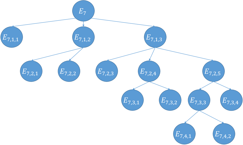
Figure 13: Tree $E_{7}$: source and destination roads are on two perpendicular roads and the destination road is charging.

(a) Event $E_{7,1,1}$

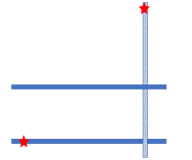
(b) Event $E_{7,2,1}$

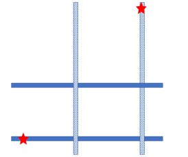
(c) Event $E_{7,2,2}$

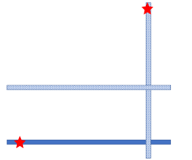
(d) Event $E_{7,2,3}$

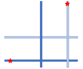
(e) Event $E_{7,2,4}$

(f) Event $E_{7,3,3}$

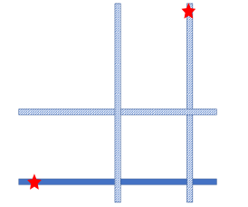
(g) Event $E_{7,3,4}$

(h)

Figure 14: Subcases of tree $E_{7}$.

• Event $E_{7,1,1}$:
  Description: If there are no horizontal roads between S and D, as shown in Fig. 14a;
  Event $L_{7,1}=E_{7,1,1}\cap E_{7}$;
  Probability: $\mathbb{P}(E_{7,1,1}|E_{7})=e^{-\lambda d_{v}}$, $\mathbb{P}(L_{7,1})=\mathbb{P}(E_{7,1,1}|E_{7})\mathbb{P}(E_{7})$;
  Action: We simply take the source road then the destination road.

  $$\mathbb{P}(D_{n}<x|L_{7,1})=\mathbb{P}(D_{n}<x|E_{7,1,1},E_{7})=\mathbbm{1}\{x>d_{h}\}.$$

• Event $E_{7,1,2}$:
  Description: If there are no horizontal charging roads but at least one horizontal non-charging road between S and D;
  Probability: $\mathbb{P}(E_{7,1,2}|E_{7})=e^{-\lambda pd_{v}}(1-e^{-\lambda(1-p)d_{v}})$.

  • Event $E_{7,2,1}$:
    Description: If there are no vertical charging roads between S and D, as shown in Fig. 14b;
    Event $L_{7,2}=E_{7,2,1}\cap E_{7,1,2}\cap E_{7}$;
    Probability: $\mathbb{P}(E_{7,2,1}|E_{7,1,2},E_{7})=e^{-\lambda pd_{h}}$, $\mathbb{P}(L_{7,2})=\mathbb{P}(E_{7,2,1}|E_{7,1,2},E_{7})\mathbb{P}(E_{7,1,2}|E_{7})\mathbb{P}(E_{7})$;
    Action: We simply take the source road then the destination road. $\mathbb{P}(D_{n}<x|L_{7,2})=\mathbb{P}(D_{n}<x|E_{7,2,1},E_{7,1,2},E_{7})=\mathbbm{1}\{x>d_{h}\}.$

  • Event $E_{7,2,2}$:
    Description: If there is at least one vertical charging road between S and D, as shown in Fig. 14c;
    Event $L_{7,3}=E_{7,2,2}\cap E_{7,1,2}\cap E_{7}$;
    Probability: $\mathbb{P}(E_{7,2,2}|E_{7,1,2},E_{7})=1-e^{-\lambda pd_{h}}$,
    $\mathbb{P}(L_{7,3})=\mathbb{P}(E_{7,2,2}|E_{7,1,2},E_{7})\mathbb{P}(E_{7,1,2}|E_{7})\mathbb{P}(E_{7})$;
    Action: We take the nearest vertical charging road.

    $$\mathbb{P}(D_{n}<x|L_{7,3})=\mathbb{P}(D_{n}<x|E_{7,2,2},E_{7,1,2},E_{7})$$

    $$=\mathbb{P}(D_{n}<x|D_{\mathrm{N-HNC}}<d_{v},D_{\mathrm{N-HC}}>d_{v},D_{\mathrm{N-VC}}<d_{h})$$

    $$=\mathbb{P}(D_{\mathrm{N-VC}}<x|D_{\mathrm{N-HNC}}<d_{v},D_{\mathrm{N-HC}}>d_{v},$$

    $$D_{\mathrm{N-VC}}<d_{h})\mathbbm{1}\{x<d_{h}\}+\mathbbm{1}\{x>d_{h}\}$$

    $$=\frac{F_{D_{\mathrm{N-VC}}}(x)}{F_{D_{\mathrm{N-VC}}}(d_{h})}\mathbbm{1}\{x<d_{h}\}+\mathbbm{1}\{x>d_{h}\}.$$ (39)

• Event $E_{7,1,3}$:
  Description: If there is at least one horizontal charging road between S and D;
  Probability: $\mathbb{P}(E_{7,1,3}|E_{7})=1-e^{-\lambda pd_{v}}$.

  • Event $E_{7,2,3}$:
    Description: If there are no vertical roads between S and D, as shown in Fig. 14d;
    Event $L_{7,4}=E_{7,2,3}\cap E_{7,1,3}\cap E_{7}$;
    Probability: $\mathbb{P}(E_{7,2,3}|E_{7,1,3},E_{7})=e^{-\lambda d_{h}}$,
    $\mathbb{P}(L_{7,4})=\mathbb{P}(E_{7,2,3}|E_{7,1,3},E_{7})\mathbb{P}(E_{7,1,3}|E_{7})\mathbb{P}(E_{7})$;
    Action: We simply take the source road then the destination road. $\mathbb{P}(D_{n}<x|L_{7,4})=\mathbb{P}(D_{n}<x|E_{7,2,3},E_{7,1,3},E_{7})=\mathbbm{1}\{x>d_{h}\}.$

  • Event $E_{7,2,4}$:
    Description: If there are no vertical charging roads but at least one vertical non-charging road between S and D, as shown in Fig. 14e;
    Probability: $\mathbb{P}(E_{7,2,4}|E_{7,1,3},E_{7})=e^{-\lambda pd_{h}}(1-e^{-\lambda(1-p)d_{h}})$;
    Action: We compare (i) the distance from the nearest vertical non-charging road to destination and (ii) the distance from source to the nearest horizontal charging road, to take the longer one.

    • Event $E_{7,3,1}$:
      Description: If we take the horizontal charging road;
      Event $L_{7,5}=E_{7,3,1}\cap E_{7,2,4}\cap E_{7,1,3}\cap E_{7}$;
      Probability: $\mathbb{P}(E_{7,3,1}|E_{7,2,4},E_{7,1,3},E_{7})=\int_{0}^{d_{h}}\frac{1-e^{-\lambda p(d_{h}-w)}}{1-e^{-\lambda pd_{v}}}\frac{\lambda(1-p)e^{-\lambda(1-p)w}}{1-e^{-\lambda pd_{v}}}dw$,
      $\mathbb{P}(L_{7,5})=\mathbb{P}(E_{7,3,1}|E_{7,2,4},E_{7,1,3},E_{7})\times\\ \mathbb{P}(E_{7,2,4}|E_{7,1,3},E_{7})\mathbb{P}(E_{7,1,3}|E_{7})\mathbb{P}(E_{7})$;

      $$\mathbb{P}(D_{n}<x|L_{7,5})=\mathbb{P}(D_{n}<x|E_{7,3,1},E_{7,2,4},E_{7,1,3},E_{7})$$

      $$=\mathbb{P}(D_{n}<x|D_{\mathrm{N-HC}}<d_{v},D_{\mathrm{N-VNC}}<d_{h},D_{\mathrm{N-VC}}>d_{h},$$

      $$d_{h}-D_{\mathrm{N-VNC}}>D_{\mathrm{N-HC}})$$

      $$=\mathbb{P}(D_{\mathrm{N-VNC}}+D_{\mathrm{N-HC}}<x|D_{\mathrm{N-HC}}<d_{v},D_{\mathrm{N-VNC}}<d_{h},$$

      $$D_{\mathrm{N-VC}}>d_{h},d_{h}-D_{\mathrm{N-VNC}}>D_{\mathrm{N-HC}})=$$

      $${\scriptstyle\frac{\mathbb{P}(D_{\mathrm{N-HC}}<{\rm min}(x-D_{\mathrm{N-VNC}},d_{v},d_{h}-D_{\mathrm{N-VNC}}),D_{\mathrm{N-VNC}}<d_{h},D_{\mathrm{N-VC}}>d_{h})}{\mathbb{P}(D_{\mathrm{N-HC}}<{\rm min}(d_{v},d_{h}-D_{\mathrm{N-VNC}}),D_{\mathrm{N-VNC}}<d_{h},D_{\mathrm{N-VC}}>d_{h})}}$$

      $$={\textstyle\frac{f_{11}({\rm max}(x-d_{v},0),x,x-y)+f_{11}(0,x-d_{v},d_{v})\mathbbm{1}\{x>d_{v}\}}{f_{11}({\rm max}(d_{h}-d_{v},0),d_{h},d_{h}-y)+f_{11}(0,d_{h}-d_{v},d_{v})\mathbbm{1}\{d_{h}>d_{v}\}}}\times$$

      $$\mathbbm{1}\{x<d_{h}\}+\mathbbm{1}\{x>d_{h}\}.$$ (40)

    • Event $E_{7,3,2}$:
      Description: If we take the destination vertical road;
      Event $L_{7,6}=E_{7,3,2}\cap E_{7,2,4}\cap E_{7,1,3}\cap E_{7}$;
      Probability: $\mathbb{P}(E_{7,3,2}|E_{7,2,4},E_{7,1,3},E_{7})=1-\int_{0}^{d_{h}}\frac{1-e^{-\lambda p(d_{h}-w)}}{1-e^{-\lambda pd_{v}}}\frac{\lambda(1-p)e^{-\lambda(1-p)w}}{1-e^{-\lambda pd_{v}}}dw$,
      $\mathbb{P}(L_{7,6})=\mathbb{P}(E_{7,3,2}|E_{7,2,4},E_{7,1,3},E_{7})\times\\ \mathbb{P}(E_{7,2,4}|E_{7,1,3},E_{7})\mathbb{P}(E_{7,1,3}|E_{7})\mathbb{P}(E_{7})$; $\mathbb{P}(D_{n}<x|L_{7,6})=\mathbb{P}(D_{n}<x|E_{7,3,2},E_{7,2,4},E_{7,1,3},E_{7})=\mathbbm{1}\{x>d_{h}\}.$

  • Event $E_{7,2,5}$:
    Description: If there is at least one vertical charging road between S and D;
    Probability: $\mathbb{P}(E_{7,2,5}|E_{7,1,3},E_{7})=1-e^{-\lambda pd_{h}}$.

    • Event $E_{7,3,3}$:
      Description: If there exists at least one vertical non-charging road before the nearest vertical charging road from source, as shown in Fig. 14f;
      Probability: $\mathbb{P}(E_{7,3,3}|E_{7,2,5},E_{7,1,3},E_{7})=1-\frac{p-pe^{-\lambda d_{h}}}{1-e^{-\lambda pd_{h}}}$;
      Action: we compare (i) the distance between the nearest vertical charging road and the nearest vertical non-charging road, and (ii) the vertical distance between the nearest horizontal charging road and source, to take the longer one.

      • Event $E_{7,4,1}$:
        Description: If we take the nearest horizontal charging road;
        Event $L_{7,7}=E_{7,4,1}\cap E_{7,3,3}\cap E_{7,2,5}\cap E_{7,1,3}\cap E_{7}$;
        Probability: $\mathbb{P}(E_{7,4,1}|E_{7,3,3},E_{7,2,5},E_{7,1,3},E_{7})=1-\int_{0}^{d_{v}}F_{X_{1}}(x)f_{D_{\mathrm{N-HC}}(x)}{\rm d}x$;
        $\mathbb{P}(L_{7,7})=\mathbb{P}(E_{7,4,1}|E_{7,3,3},E_{7,2,5},E_{7,1,3},E_{7})\times\\ \mathbb{P}(E_{7,3,3}|E_{7,2,5},E_{7,1,3},E_{7})\times\\ \mathbb{P}(E_{7,2,5}|E_{7,1,3},E_{7})\mathbb{P}(E_{7,1,3}|E_{7})\mathbb{P}(E_{7})$;

        $$\mathbb{P}(D_{n}<x|L_{7,7})=\mathbb{P}(D_{n}<x|E_{7,4,1},E_{7,3,3},E_{7,2,5},E_{7,1,3},E_{7})$$

        $$=\mathbb{P}(D_{\mathrm{N-VNC}}+D_{\mathrm{N-HC}}<x|D_{\mathrm{N-VC}}<d_{h},$$

        $$D_{\mathrm{N-VNC}}<D_{\mathrm{N-VC}},D_{\mathrm{N-VC}}-D_{\mathrm{N-VNC}}>D_{\mathrm{N-HC}})\times$$

        $$\mathbbm{1}\{x<d_{h}\}+\mathbbm{1}\{x>d_{h}\}$$

        $$=\frac{f_{12}(0,x,x,d_{h},x-t)+f_{12}(0,x,0,x,y-t)}{f_{13}(0,d_{h},0,d_{h}-t,d_{h},t+y)}\mathbbm{1}\{x<d_{h}\}$$

        $$+\mathbbm{1}\{x>d_{h}\}.$$ (41)

        The proof for $\mathbb{P}(D_{n}<x|E_{7,4,1},E_{7,3,3},E_{7,2,5},E_{7,1,3},E_{7})$ is similar to that of
        $\mathbb{P}(D_{n}<x|E_{3,4,3},E_{3,3,3},E_{3,2,4},E_{3,1,4},E_{3})$ given in (· ‣ * ‣ – ‣ • ‣ D).

      • Event $E_{7,4,2}$:
        Description: If we take the nearest vertical charging road;
        Event $L_{7,8}=E_{7,4,2}\cap E_{7,3,3}\cap E_{7,2,5}\cap E_{7,1,3}\cap E_{7}$;
        Probability: $\mathbb{P}(E_{7,4,2}|E_{7,3,3},E_{7,2,5},E_{7,1,3},E_{7})=\int_{0}^{d_{v}}F_{X_{1}}(x)f_{D_{\mathrm{N-HC}}(x)}{\rm d}x$;
        $\mathbb{P}(L_{7,8})=\mathbb{P}(E_{7,4,2}|E_{7,3,3},E_{7,2,5},E_{7,1,3},E_{7})\times\\ \mathbb{P}(E_{7,3,3}|E_{7,2,5},E_{7,1,3},E_{7})\times\\ \mathbb{P}(E_{7,2,5}|E_{7,1,3},E_{7})\mathbb{P}(E_{7,1,3}|E_{7})\mathbb{P}(E_{7})$;

        $$\mathbb{P}(D_{n}<x|L_{7,8})=\mathbb{P}(D_{n}<x|E_{7,4,2},E_{7,3,3},E_{7,2,5},E_{7,1,3},E_{7})$$

        $$=\mathbb{P}(D_{\mathrm{N-VC}}<x|D_{\mathrm{N-VC}}<d_{h},D_{\mathrm{N-VNC}}<D_{\mathrm{N-VC}},$$

        $$D_{\mathrm{N-VC}}-D_{\mathrm{N-VNC}}<D_{\mathrm{N-HC}})\mathbbm{1}\{x<d_{h}\}+\mathbbm{1}\{x>d_{h}\}$$

        $$={\textstyle\frac{f_{13}(0,\infty,0,{\rm max}(x-t,0),y+t,y)-f_{13}(0,\infty,{\rm max}(x-t,0),x,x,y)}{f_{13}(0,\infty,0,{\rm max}(d_{h}-t,0),y+t,y)-f_{13}(0,\infty,{\rm max}(d_{h}-t,0),d_{h},x,y)}}\times$$

        $$\mathbbm{1}\{x<d_{h}\}+\mathbbm{1}\{x>d_{h}\}.$$ (42)

        The proof for $\mathbb{P}(D_{n}<x|E_{7,4,2},E_{7,3,3},E_{7,2,5},E_{7,1,3},E_{7})$ is similar to that of
        $\mathbb{P}(D_{n}<x|E_{3,4,4},E_{3,3,3},E_{3,2,4},E_{3,1,4},E_{3})$ given in (· ‣ * ‣ – ‣ • ‣ D).

    • Event $E_{7,3,4}$:
      Description: If there exists no vertical non-charging road before the nearest vertical charging road from source, as shown in Fig. 14g;
      Event $L_{7,9}=E_{7,3,4}\cap E_{7,2,5}\cap E_{7,1,3}\cap E_{7}$;
      Probability: $\mathbb{P}(E_{7,3,4}|E_{7,2,5},E_{7,1,3},E_{7})=\frac{p-pe^{-\lambda d_{h}}}{1-e^{-\lambda pd_{v}}}$,
      $\mathbb{P}(L_{7,9})=\mathbb{P}(E_{7,3,4}|E_{7,2,5},E_{7,1,3},E_{7})\times\\ \mathbb{P}(E_{7,2,5}|E_{7,1,3},E_{7})\mathbb{P}(E_{7,1,3}|E_{7})\mathbb{P}(E_{7})$;
      Action: we simply go with the nearest vertical charging road.

      $$\mathbb{P}(D_{n}<x|L_{7,9})=\mathbb{P}(D_{n}<x|E_{7,3,4},E_{7,2,5},E_{7,1,3},E_{7})$$

      $$=\mathbb{P}(D_{\mathrm{N-VC}}<x|D_{\mathrm{N-VC}}<D_{\mathrm{N-VNC}},D_{\mathrm{N-VC}}<d_{h})$$

      $$=\frac{\mathbb{P}(D_{\mathrm{N-VC}}<{\rm min}(x,D_{\mathrm{N-VNC}})}{\mathbb{P}(D_{\mathrm{N-VC}}<{\rm min}(D_{\mathrm{N-VNC}},d_{h}))}\mathbbm{1}\{x<d_{h}\}+$$

      $$\mathbbm{1}\{x>d_{h}\}$$

      $$=\frac{f_{11}(0,x,y)+f_{11}(x,\infty,x)}{f_{11}(0,d_{h},y)+f_{11}(d_{h},\infty,d_{h})}\mathbbm{1}\{x<d_{h}\}+\mathbbm{1}\{x>d_{h}\}.$$ (43)

      The proof for $\mathbb{P}(D_{n}<x|E_{7,3,4},E_{7,2,5},E_{7,1,3},E_{7})$ is similar to that of $\mathbb{P}(D_{n}<x|E_{3,3,4},E_{3,2,4},E_{3,1,4},E_{3})$ given in (* ‣ – ‣ • ‣ D).

∎

Appendix H proof of Lemma 8

In this appendix, we first provide the complete form of Lemma 8, i.e., the distribution of $D_{n}$ given $E_{8}$, as follows:

$$\mathbb{P}(D_{n}<x|E_{8})\mathbb{P}(E_{8})=\sum_{i=1}^{5}C_{i},$$ (44)

where

$$C_{1}=$$

$$\biggl{(}\frac{F_{D_{\mathrm{N-VC}}}(x)}{F_{D_{\mathrm{N-VC}}}(d_{h})}\mathbbm{1}\{x<d_{h}\}+\mathbbm{1}\{x>d_{h}\}\biggr{)}(1-e^{-\lambda pd_{h}})\times$$

$$e^{-\lambda pd_{v}}(1-e^{-\lambda(1-p)d_{v}})\frac{(1-p)^{2}}{2},$$

$$C_{2}=$$

$$\biggl{(}{\textstyle\frac{f_{11}({\rm max}(x-d_{v},0),{\rm min}(x,d_{h}),x-o)+f_{11}(0,{\rm min}(x-d_{v},d_{h}),d_{v})\mathbbm{1}\{x>d_{v}\}}{F_{D_{\mathrm{N-HC}}}(d_{v})F_{D_{\mathrm{N-VNC}}}(d_{h})}}$$

$$\times\mathbbm{1}\{x<d_{h}+d_{v}\}+\mathbbm{1}\{x>d_{h}+d_{v}\}\biggr{)}e^{-\lambda pd_{h}}\times$$

$$(1-e^{-\lambda(1-p)d_{h}})(1-e^{-\lambda pd_{v}})\frac{(1-p)^{2}}{2},$$

$$C_{3}=$$

$$\biggl{(}\frac{f_{12}(0,x,x,d_{h},x-t)+f_{12}(0,x,0,x,y-t)}{f_{13}(0,d_{h},0,d_{h}-t,d_{h},t+y)}\mathbbm{1}\{x<d_{h}\}$$

$$+\mathbbm{1}\{x>d_{h}\}\biggr{)}\biggl{(}1-\int_{0}^{d_{v}}F_{X_{1}}(x)f_{D_{\mathrm{N-HC}}(x)}{\rm d}x\biggr{)}\times$$

$$\biggl{(}1-\frac{p-pe^{-\lambda d_{h}}}{1-e^{-\lambda pd_{h}}}\biggr{)}(1-e^{-\lambda pd_{h}})(1-e^{-\lambda pd_{v}})\frac{(1-p)^{2}}{2},$$

$$C_{4}=$$

$$\biggl{(}{\textstyle\frac{f_{13}(0,\infty,0,{\rm max}(x-t,0),y+t,y)-f_{13}(0,\infty,{\rm max}(x-t,0),x,x,y)}{f_{13}(0,\infty,0,{\rm max}(d_{h}-t,0),y+t,y)-f_{13}(0,\infty,{\rm max}(d_{h}-t,0),d_{h},x,y)}}\times$$

$$\mathbbm{1}\{x<d_{h}\}+\mathbbm{1}\{x>d_{h}\}\biggr{)}\biggl{(}\int_{0}^{d_{v}}F_{X_{1}}(x)f_{D_{\mathrm{N-HC}}(x)}{\rm d}x\biggr{)}$$

$$\times\biggl{(}1-\frac{p-pe^{-\lambda d_{h}}}{1-e^{-\lambda pd_{h}}}\biggr{)}(1-e^{-\lambda pd_{h}})(1-e^{-\lambda pd_{v}})\frac{(1-p)^{2}}{2},$$

$$C_{5}=$$

$$\biggl{(}\frac{f_{11}(0,x,y)+f_{11}(x,\infty,x)}{f_{11}(0,d_{h},y)+f_{11}(d_{h},\infty,d_{h})}\mathbbm{1}\{x<d_{h}\}+\mathbbm{1}\{x>d_{h}\}\biggr{)}$$

$$\times\biggl{(}\frac{p-pe^{-\lambda d_{h}}}{1-e^{-\lambda pd_{h}}}\biggr{)}(1-e^{-\lambda pd_{h}})(1-e^{-\lambda pd_{v}})\frac{(1-p)^{2}}{2}.$$

Proof:

We prove (44) by further dividing it into subevents, as shown in Fig. 15, we hereby denote subevents as $E_{8,i,j}$, in which $i$ is the level of depth of the event in the probability tree and $j$ is the index of the event at that level. Representative figures for $E_{8}$ are shown in Fig. 16. The distribution of $D_{n}$ given $E_{8}$ can be derived as follows:

$$\mathbb{P}(D_{n}<x|E_{8})\mathbb{P}(E_{8})=\sum_{i=1}^{N_{8}}\mathbb{P}(D_{n}<x|L_{8,i})\mathbb{P}(L_{8,i}),$$

where $N_{8}$ denotes the number of leaves of tree $E_{8}$, i.e., $N_{8}=8$, and $L_{8,i}$’s are successive events ending at the leaves of tree $E_{8}$ as shown in Fig. 15. The definition for each event $L_{8,i}$ will be given in more details as we visit each leaf of the tree.

Figure 15: Tree $E_{8}$: source and destination roads are on two perpendicular roads and both are not charging.

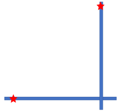
(a) Event $E_{8,1,1}$

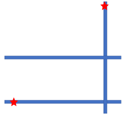
(b) Event $E_{8,2,1}$

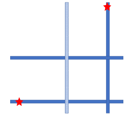
(c) Event $E_{8,2,2}$

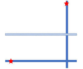
(d) Event $E_{8,2,3}$

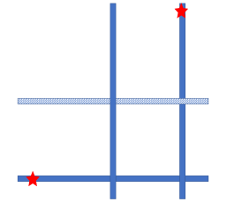
(e) Event $E_{8,2,4}$

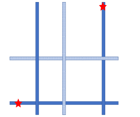
(f) Event $E_{8,3,1}$

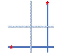
(g) Event $E_{8,3,2}$

(h)

Figure 16: Subcases of tree $E_{8}$.

• Event $E_{8,1,1}$:
  Description: If there are no horizontal roads between S and D, as shown in Fig. 16a;
  Event $L_{8,1}=E_{8,1,1}\cap E_{8}$;
  Probability: $\mathbb{P}(E_{8,1,1}|E_{8})=e^{-\lambda d_{v}}$, $\mathbb{P}(L_{8,1})=\mathbb{P}(E_{8,1,1}|E_{8})\mathbb{P}(E_{8})$;
  Action: We simply take the source road then the destination road.

  $$\mathbb{P}(D_{n}<x|L_{8,1})=\mathbb{P}(D_{n}<x|E_{8,1,1},E_{8})=0.$$

• Event $E_{8,1,2}$:
  Description: If there are no horizontal charging roads but at least one horizontal non-charging road between S and D;
  Probability: $\mathbb{P}(E_{8,1,2}|E_{8})=e^{-\lambda pd_{v}}(1-e^{-\lambda(1-p)d_{v}})$.

  • Event $E_{8,2,1}$:
    Description: If there are no vertical charging roads between S and D, as shown in Fig. 16b;
    Event $L_{8,2}=E_{8,2,1}\cap E_{8,1,2}\cap E_{8}$;
    Probability: $\mathbb{P}(E_{8,2,1}|E_{8,1,2},E_{8})=e^{-\lambda pd_{h}}$,
    $\mathbb{P}(L_{8,2})=\mathbb{P}(E_{8,2,1}|E_{8,1,2},E_{8})\mathbb{P}(E_{8,1,2}|E_{8})\mathbb{P}(E_{8})$;
    Action: We take the source road then the destination road.

    $$\mathbb{P}(D_{n}<x|L_{8,2})=\mathbb{P}(D_{n}<x|E_{8,2,1},E_{8,1,2},E_{8})=0.$$

  • Event $E_{8,2,2}$:
    Description: If there is at least one vertical charging road between S and D, as shown in Fig. 16c;
    Event $L_{8,3}=E_{8,2,2}\cap E_{8,1,2}\cap E_{8}$;
    Probability: $\mathbb{P}(E_{8,2,2}|E_{8,1,2},E_{8})=1-e^{-\lambda pd_{h}}$,
    $\mathbb{P}(L_{8,3})=\mathbb{P}(E_{8,2,2}|E_{8,1,2},E_{8})\mathbb{P}(E_{8,1,2}|E_{8})\mathbb{P}(E_{8})$;
    Action: We go to the nearest vertical charging road from source, then switch to the furthest horizontal non-charging road from source.

    $$\mathbb{P}(D_{n}<x|L_{8,3})=\mathbb{P}(D_{n}<x|E_{8,2,2},E_{8,1,2},E_{8})$$

    $$=\frac{F_{D_{\mathrm{N-VC}}}(x)}{F_{D_{\mathrm{N-VC}}}(d_{h})}\mathbbm{1}\{x<d_{h}\}+\mathbbm{1}\{x>d_{h}\}.$$ (45)

    The proof for $\mathbb{P}(D_{n}<x|E_{8,2,2},E_{8,1,2},E_{8})$ is similar to that of $\mathbb{P}(D_{n}<x|E_{7,2,2},E_{7,1,2},E_{7})$ given in (– ‣ • ‣ G).

• Event $E_{8,1,3}$:
  Description: If there is at least one horizontal charging road between S and D;
  Probability: $\mathbb{P}(E_{8,1,3}|E_{8})=1-e^{-\lambda pd_{v}}$.

  • Event $E_{8,2,3}$:
    Description: If there are no vertical roads between S and D, as shown in Fig. 16d;
    Event $L_{8,4}=E_{8,2,3}\cap E_{8,1,3}\cap E_{8}$;
    Probability: $\mathbb{P}(E_{8,2,3}|E_{8,1,3},E_{8})=e^{-\lambda d_{h}}$,
    $\mathbb{P}(L_{8,4})=\mathbb{P}(E_{8,2,3}|E_{8,1,3},E_{8})\mathbb{P}(E_{8,1,3}|E_{8})\mathbb{P}(E_{8})$;
    Action: We take the source road then the destination road.

    $$\mathbb{P}(D_{n}<x|L_{8,4})=\mathbb{P}(D_{n}<x|E_{8,2,3},E_{8,1,3},E_{8})=0.$$

  • Event $E_{8,2,4}$:
    Description: If there are no vertical charging roads but at least one vertical non-charging road between S and D, as shown in Fig. 16e;
    Event $L_{8,5}=E_{8,2,4}\cap E_{8,1,3}\cap E_{8}$;
    Probability: $\mathbb{P}(E_{8,2,4}|E_{8,1,3},E_{8})=e^{-\lambda pd_{h}}(1-e^{-\lambda(1-p)d_{h})})$,
    $\mathbb{P}(L_{8,5})=\mathbb{P}(E_{8,2,4}|E_{8,1,3},E_{8})\mathbb{P}(E_{8,1,3}|E_{8})\mathbb{P}(E_{8})$;
    Action: We go to the nearest vertical non-charging road, then switch to any horizontal charging road between S and D.

    $$\mathbb{P}(D_{n}<x|L_{8,5})=\mathbb{P}(D_{n}<x|E_{8,2,4},E_{8,1,3},E_{8})$$

    $$=\mathbb{P}(D_{\mathrm{N-VNC}}+D_{\mathrm{N-HC}}<x|D_{\mathrm{N-HC}}<d_{v},D_{\mathrm{N-VC}}>d_{h},$$

    $$D_{\mathrm{N-VNC}}<d_{h})$$

    $$={\textstyle\frac{\mathbb{P}(D_{\mathrm{N-HC}}<{\rm min}(x-D_{\mathrm{N-VNC}},d_{v}),D_{\mathrm{N-VC}}>d_{h},D_{\mathrm{N-VNC}}<d_{h})}{\mathbb{P}(D_{\mathrm{N-HC}}<d_{v},D_{\mathrm{N-VNC}}<d_{h}<D_{\mathrm{N-VC}})}}$$

    $$={\textstyle\frac{f_{11}({\rm max}(x-d_{v},0),{\rm min}(x,d_{h}),x-o)+f_{11}(0,{\rm min}(x-d_{v},d_{h}),d_{v})\mathbbm{1}\{x>d_{v}\}}{F_{D_{\mathrm{N-HC}}}(d_{v})F_{D_{\mathrm{N-VNC}}}(d_{h})}}$$

    $$\times\mathbbm{1}\{x<d_{h}+d_{v}\}+\mathbbm{1}\{x>d_{h}+d_{v}\}.$$ (46)

  • Event $E_{8,2,5}$:
    Description: If there is at least one vertical charging road between S and D;
    Probability: $\mathbb{P}(E_{8,2,5}|E_{8,1,3},E_{8})=1-e^{-\lambda pd_{h}}$.

    • Event $E_{8,3,1}$:
      Description: If there exists at least one vertical non-charging road before the nearest vertical charging road from S, as shown in Fig. 16f;
      Probability: $\mathbb{P}(E_{8,3,1}|E_{8,2,5},E_{8,1,3},E_{8})=1-\frac{p-pe^{-\lambda d_{h}}}{1-e^{-\lambda pd_{h}}}$;
      Action: we compare (i) the distance between the nearest vertical charging road and the nearest vertical non-charging road, and (ii) the vertical distance between the nearest horizontal charging road and source, to take the longer one.

      • Event $E_{8,4,1}$:
        Description: If we take the nearest horizontal charging road;
        Event $L_{8,6}=E_{8,4,1}\cap E_{8,3,1}\cap E_{8,2,5}\cap E_{8,1,3}\cap E_{8}$;
        Probability: $\mathbb{P}(E_{8,4,1}|E_{8,3,1},E_{8,2,5},E_{8,1,3},E_{8})=1-\int_{0}^{d_{v}}F_{X_{1}}(x)f_{D_{\mathrm{N-HC}}(x)}{\rm d}x$;
        $\mathbb{P}(L_{8,6})=\mathbb{P}(E_{8,4,1}|E_{8,3,1},E_{8,2,5},E_{8,1,3},E_{8})\times\\ \mathbb{P}(E_{8,3,1}|E_{8,2,5},E_{8,1,3},E_{8})\times\\ \mathbb{P}(E_{8,2,5}|E_{8,1,3},E_{8})\mathbb{P}(E_{8,1,3}|E_{8})\mathbb{P}(E_{8})$;

        $$\mathbb{P}(D_{n}<x|L_{8,6})=\mathbb{P}(D_{n}<x|E_{8,4,1},E_{8,3,1},E_{8,2,5},E_{8,1,3},E_{8})$$

        $$=\frac{f_{12}(0,x,x,d_{h},x-t)+f_{12}(0,x,0,x,y-t)}{f_{13}(0,d_{h},0,d_{h}-t,d_{h},t+y)}\mathbbm{1}\{x<d_{h}\}$$

        $$+\mathbbm{1}\{x>d_{h}\}$$ (47)

        The proof for $\mathbb{P}(D_{n}<x|E_{8,4,1},E_{8,3,1},E_{8,2,5},E_{8,1,3},E_{8})$ is similar to that of
        $\mathbb{P}(D_{n}<x|E_{7,4,1},E_{7,3,3},E_{7,2,5},E_{7,1,3},E_{7})$ given in (· ‣ * ‣ – ‣ • ‣ G).

      • Event $E_{8,4,2}$:
        Description: If we take the nearest vertical charging road;
        Event $L_{8,7}=E_{8,4,2}\cap E_{8,3,1}\cap E_{8,2,5}\cap E_{8,1,3}\cap E_{8}$;
        Probability: $\mathbb{P}(E_{8,4,2}|E_{8,3,1}|E_{8,2,5},E_{8,1,3},E_{8})=\int_{0}^{d_{v}}F_{X_{1}}(x)f_{D_{\mathrm{N-HC}}(x)}{\rm d}x$;
        $\mathbb{P}(L_{8,7})=\mathbb{P}(E_{8,4,2}|E_{8,3,1},E_{8,2,5},E_{8,1,3},E_{8})\times\\ \mathbb{P}(E_{8,3,1}|E_{8,2,5},E_{8,1,3},E_{8})\times\\ \mathbb{P}(E_{8,2,5}|E_{8,1,3},E_{8})\mathbb{P}(E_{8,1,3}|E_{8})\mathbb{P}(E_{8})$;

        $$\mathbb{P}(D_{n}<x|L_{8,7})=\mathbb{P}(D_{n}<x|E_{8,4,2},E_{8,3,1},E_{8,2,5},E_{8,1,3},E_{8})$$

        $$={\textstyle\frac{f_{13}(0,\infty,0,{\rm max}(x-t,0),y+t,y)-f_{13}(0,\infty,{\rm max}(x-t,0),x,x,y)}{f_{13}(0,\infty,0,{\rm max}(d_{h}-t,0),y+t,y)-f_{13}(0,\infty,{\rm max}(d_{h}-t,0),d_{h},x,y)}}\times$$

        $$\mathbbm{1}\{x<d_{h}\}+\mathbbm{1}\{x>d_{h}\}.$$ (48)

        The proof for $\mathbb{P}(D_{n}<x|E_{8,4,2},E_{8,3,1},E_{8,2,5},E_{8,1,3},E_{8})$ is similar to that of
        $\mathbb{P}(D_{n}<x|E_{7,4,2},E_{7,3,3},E_{7,2,5},E_{7,1,3},E_{7})$ given in (· ‣ * ‣ – ‣ • ‣ G).

    • Event $E_{8,3,2}$:
      Description: If there exists no vertical non-charging road before the nearest vertical charging road from source, as shown in Fig. 16g;
      Event $L_{8,8}=E_{8,3,2}\cap E_{8,2,5}\cap E_{8,1,3}\cap E_{8}$;
      Probability: $\mathbb{P}(E_{8,3,2}|E_{8,2,5},E_{8,1,3},E_{8})=\frac{p-pe^{-\lambda d_{h}}}{1-e^{-\lambda pd_{h}}}$,
      $\mathbb{P}(L_{8,8})=\mathbb{P}(E_{8,3,2}|E_{8,2,5},E_{8,1,3},E_{8})\times\\ \mathbb{P}(E_{8,2,5}|E_{8,1,3},E_{8})\mathbb{P}(E_{8,1,3}|E_{8})\mathbb{P}(E_{8})$;
      Action: we simply go with the nearest vertical charging road.

      $$\mathbb{P}(D_{n}<x|L_{8,8})=\mathbb{P}(D_{n}<x|E_{8,3,2},E_{8,2,5},E_{8,1,3},E_{8})$$

      $$=\frac{f_{11}(0,x,y)+f_{11}(x,\infty,x)}{f_{11}(0,d_{h},y)+f_{11}(d_{h},\infty,d_{h})}\mathbbm{1}\{x<d_{h}\}+\mathbbm{1}\{x>d_{h}\}.$$ (49)

      The proof for $\mathbb{P}(D_{n}<x|E_{8,3,2},E_{8,2,5},E_{8,1,3},E_{8})$ is similar to that of $\mathbb{P}(D_{n}<x|E_{7,3,4},E_{7,2,5},E_{7,1,3},E_{7})$ given in (* ‣ – ‣ • ‣ G).

∎

Appendix I Proof of Theorem 2

In this appendix, we outline the proof for the probability that any given trip passes through at least one charging road, i.e., $\mathbb{P}(T_{c})$.
$\mathbb{P}(\overline{T_{c}}|E_{4})\mathbb{P}(E_{4})$:

$$\mathbb{P}(\overline{T_{c}}|E_{4})\mathbb{P}(E_{4})=[\mathbb{P}(E_{4,1,1})(1-p)+\mathbb{P}(E_{4,1,2})$$

$$+\mathbb{P}(E_{4,1,4})\mathbb{P}(E_{4,2,1})]\mathbb{P}(E_{4})$$

$$=[e^{-\lambda d_{v}}(1-p)+\lambda(1-p)d_{v}e^{-\lambda(1-p)d_{v}}e^{-\lambda pd_{v}}$$

$$+e^{-\lambda pd_{v}}(1-e^{-\lambda(1-p)d_{v}}-\lambda(1-p)d_{v}e^{-\lambda(1-p)d_{v}})e^{-\lambda pd_{h}}]$$

$$\times(1-p)^{2}.$$ (50)

$\mathbb{P}(\overline{T_{c}}|E_{8})\mathbb{P}(E_{8})$:

$$\mathbb{P}(\overline{T_{c}}|E_{8})\mathbb{P}(E_{8})=[\mathbb{P}(E_{8,1,1})+\mathbb{P}(E_{8,1,2})\mathbb{P}(E_{8,2,1})$$

$$+\mathbb{P}(E_{8,1,3})\mathbb{P}(E_{8,2,3})]\mathbb{P}(E_{8})$$

$$=[e^{-\lambda d_{v}}+e^{-\lambda pd_{v}}(1-e^{-\lambda(1-p)d_{v}})e^{-\lambda pd_{h}}$$

$$+(1-e^{-\lambda pd_{v}})e^{-\lambda d_{h}}](1-p)^{2}.$$ (51)

Duc Minh Nguyen was born in Hanoi, Vietnam. He received the M.S. degree in Electrical and Computer Engineering from King Abdullah University of Science and Technology (KAUST), Saudi Arabia, and the B.Eng. degree in Mobile Systems Engineering from Dankook University, Republic of Korea, in 2020 and 2018, respectively. He is currently pursuing the Ph.D. degree with the Computer, Electrical and Mathematical Science and Engineering Division, KAUST, Saudi Arabia. His research interests include social/vehicular networks analysis, data mining, and machine learning.

Mustafa A. Kishk [S’16, M’18] is a postdoctoral research fellow in the communication theory lab at King Abdullah University of Science and Technology (KAUST). He received his B.Sc. and M.Sc. degree from Cairo University in 2013 and 2015, respectively, and his Ph.D. degree from Virginia Tech in 2018. His current research interests include stochastic geometry, energy harvesting wireless networks, UAV-enabled communication systems, and satellite communications.

Mohamed-Slim Alouini [S’94-M’98-SM’03-F’09] was born in Tunis, Tunisia. He received the Ph.D. degree in Electrical Engineering from the California Institute of Technology (Caltech), Pasadena, CA, USA, in 1998. He served as a faculty member in the University of Minnesota, Minneapolis, MN, USA, then in the Texas A&M University at Qatar, Education City, Doha, Qatar before joining King Abdullah University of Science and Technology (KAUST), Thuwal, Makkah Province, Saudi Arabia as a Professor of Electrical Engineering in 2009. His current research interests include the modeling, design, and performance analysis of wireless communication systems.

References

- [1] D. Sperling, Future drive: Electric vehicles and sustainable transportation. Island Press, 2013.
- [2] M. Catenacci, E. Verdolini, V. Bosetti, and G. Fiorese, “Going electric: Expert survey on the future of battery technologies for electric vehicles,” Energy Policy, vol. 61, pp. 403 – 413, 2013.
- [3] L. Lu, X. Han, J. Li, J. Hua, and M. Ouyang, “A review on the key issues for lithium-ion battery management in electric vehicles,” Journal of Power Sources, vol. 226, pp. 272 – 288, 2013.
- [4] B. Nykvist and M. Nilsson, “Rapidly falling costs of battery packs for electric vehicles,” Nature climate change, vol. 5, no. 4, pp. 329–332, 2015.
- [5] A. Abdalrahman and W. Zhuang, “PEV charging infrastructure siting based on spatial–temporal traffic flow distribution,” IEEE Transactions on Smart Grid, vol. 10, no. 6, pp. 6115–6125, Nov. 2019.
- [6] A. Abdalrahman and W. Zhuang, “A survey on PEV charging infrastructure: Impact assessment and planning,” Energies, vol. 10, Oct. 2017.
- [7] A. Abdalrahman and W. Zhuang, “QoS-aware capacity planning of networked PEV charging infrastructure,” IEEE Open Journal of Vehicular Technology, vol. 1, pp. 116–129, Mar. 2020.
- [8] R. Atat, M. Ismail, and E. Serpedin, “Stochastic geometry planning of electric vehicles charging stations,” in ICASSP 2020 - 2020 IEEE International Conference on Acoustics, Speech and Signal Processing (ICASSP), April 2020, pp. 3062–3066.
- [9] C. Panchal, S. Stegen, and J. Lu, “Review of static and dynamic wireless electric vehicle charging system,” Engineering Science and Technology, an International Journal, vol. 21, no. 5, pp. 922 – 937, 2018.
- [10] H. H. Wu, A. Gilchrist, K. Sealy, P. Israelsen, and J. Muhs, “A review on inductive charging for electric vehicles,” in 2011 IEEE International Electric Machines Drives Conference (IEMDC), May 2011, pp. 143–147.
- [11] T. Stamati and P. Bauer, “On-road charging of electric vehicles,” in 2013 IEEE Transportation Electrification Conference and Expo (ITEC), June 2013, pp. 1–8.
- [12] C. C. Mi, G. Buja, S. Y. Choi, and C. T. Rim, “Modern advances in wireless power transfer systems for roadway powered electric vehicles,” IEEE Transactions on Industrial Electronics, vol. 63, no. 10, pp. 6533–6545, Oct. 2016.
- [13] S. Y. Choi, B. W. Gu, S. Y. Jeong, and C. T. Rim, “Advances in wireless power transfer systems for roadway-powered electric vehicles,” IEEE Journal of Emerging and Selected Topics in Power Electronics, vol. 3, no. 1, pp. 18–36, 2015.
- [14] J. T. Boys and G. A. Covic, “The inductive power transfer story at the University of Auckland,” IEEE Circuits and Systems Magazine, vol. 15, no. 2, pp. 6–27, 2015.
- [15] O. C. Onar, J. M. Miller, S. L. Campbell, C. Coomer, C. P. White, and L. E. Seiber, “Oak Ridge national laboratory wireless power transfer development for sustainable campus initiative,” in 2013 IEEE Transportation Electrification Conference and Expo (ITEC), June 2013, pp. 1–8.
- [16] Y. J. Jang, E. S. Suh, and J. W. Kim, “System architecture and mathematical models of electric transit bus system utilizing wireless power transfer technology,” IEEE Systems Journal, vol. 10, no. 2, pp. 495–506, Jun. 2016.
- [17] M. Budhia, J. T. Boys, G. A. Covic, and C. Huang, “Development of a single-sided flux magnetic coupler for electric vehicle IPT charging systems,” IEEE Transactions on Industrial Electronics, vol. 60, no. 1, pp. 318–328, Jan. 2013.
- [18] O. C. Onar, S. L. Campbell, L. E. Seiber, C. P. White, and M. Chinthavali, “A high-power wireless charging system development and integration for a Toyota RAV4 electric vehicle,” in 2016 IEEE Transportation Electrification Conference and Expo (ITEC), June 2016, pp. 1–8.
- [19] O. C. Onar, M. Chinthavali, S. L. Campbell, L. E. Seiber, C. P. White, and V. P. Galigekere, “Modeling, simulation, and experimental verification of a 20-kw series-series wireless power transfer system for a Toyota RAV4 electric vehicle,” in 2018 IEEE Transportation Electrification Conference and Expo (ITEC), June 2018, pp. 874–880.
- [20] “Qualcomm demonstrates dynamic electric vehicle charging,” https://www.qualcomm.com/news/releases/2017/05/18/qualcomm-demonstrates-dynamic-electric-vehicle-charging, accessed: 2020-03-18.
- [21] “Witricity acquires Qualcomm Halo,” https://witricity.com/witricity-acquires-qualcomm-halo, accessed: 2020-03-18.
- [22] J. Eisner, S. Funke, and S. Storandt, “Optimal route planning for electric vehicles in large networks,” in Twenty-Fifth AAAI Conference on Artificial Intelligence, 2011.
- [23] A. Sarker, H. Shen, and J. A. Stankovic, “MORP: Data-driven multi-objective route planning and optimization for electric vehicles,” Proceedings of the ACM on Interactive, Mobile, Wearable and Ubiquitous Technologies, vol. 1, no. 4, Jan. 2018.
- [24] L. Fu, D. Sun, and L. R. Rilett, “Heuristic shortest path algorithms for transportation applications: state of the art,” Computers & Operations Research, vol. 33, no. 11, pp. 3324–3343, 2006.
- [25] W. Zeng and R. L. Church, “Finding shortest paths on real road networks: the case for a,” International journal of geographical information science, vol. 23, no. 4, pp. 531–543, 2009.
- [26] M. Hua and J. Pei, “Probabilistic path queries in road networks: traffic uncertainty aware path selection,” in Proceedings of the 13th International Conference on Extending Database Technology, 2010, pp. 347–358.
- [27] W. S. Kendall, “Geodesics and flows in a Poissonian city,” The Annals of Applied Probability, vol. 21, no. 3, pp. 801–842, 2011.
- [28] R. G. Leal, “Mean traffic behaviour in Poissonian cities,” Ph.D. dissertation, University of Warwick, 2018.
- [29] H. S. Dhillon and V. V. Chetlur, Poisson Line Cox Process: Foundations and Applications to Vehicular Networks. Morgan & Claypool, 2020.
- [30] M. Haenggi, Stochastic Geometry for Wireless Networks. Cambridge University Press, 2012.
- [31] G. Baics and L. Meisterlin, “The grid as algorithm for land use: a reappraisal of the 1811 manhattan grid,” Planning Perspectives, vol. 34, no. 3, pp. 391–414, 2019.
- [32] G. D. Suttles, The man-made city: The land-use confidence game in Chicago. University of Chicago Press, 1990.
- [33] L. Berelowitz, Dream city: Vancouver and the global imagination. Douglas & McIntyre, 2010.
- [34] K. Al Sayed, A. Turner, and S. Hanna, “Cities as emergent models: the morphological logic of manhattan and barcelona.” Royal Institute of Technology (KTH), 2009.
- [35] J. Dai and D. C. Ludois, “A survey of wireless power transfer and a critical comparison of inductive and capacitive coupling for small gap applications,” IEEE Transactions on Power Electronics, vol. 30, no. 11, pp. 6017–6029, 2015.
- [36] P. Machura and Q. Li, “A critical review on wireless charging for electric vehicles,” Renewable and Sustainable Energy Reviews, vol. 104, pp. 209 – 234, Apr. 2019.
- [37] M. Yilmaz, V. T. Buyukdegirmenci, and P. T. Krein, “General design requirements and analysis of roadbed inductive power transfer system for dynamic electric vehicle charging,” in 2012 IEEE Transportation Electrification Conference and Expo (ITEC), June 2012, pp. 1–6.
- [38] W. Zhang, S. Wong, C. K. Tse, and Q. Chen, “An optimized track length in roadway inductive power transfer systems,” IEEE Journal of Emerging and Selected Topics in Power Electronics, vol. 2, no. 3, pp. 598–608, Sep. 2014.
- [39] G. R. Nagendra, G. A. Covic, and J. T. Boys, “Sizing of inductive power pads for dynamic charging of EVs on IPT highways,” IEEE Transactions on Transportation Electrification, vol. 3, no. 2, pp. 405–417, June 2017.
- [40] J. Kim, J. Kim, S. Kong, H. Kim, I. Suh, N. P. Suh, D. Cho, J. Kim, and S. Ahn, “Coil design and shielding methods for a magnetic resonant wireless power transfer system,” Proceedings of the IEEE, vol. 101, no. 6, pp. 1332–1342, 2013.
- [41] A. Sarker, C. Qiu, H. Shen, A. Gil, J. Taiber, M. Chowdhury, J. Martin, M. Devine, and A. Rindos, “An efficient wireless power transfer system to balance the state of charge of electric vehicles,” in 2016 45th International Conference on Parallel Processing (ICPP), 2016, pp. 324–333.
- [42] C. Qiu, A. Sarker, and H. Shen, “Power distribution scheduling for electric vehicles in wireless power transfer systems,” in 2017 14th Annual IEEE International Conference on Sensing, Communication, and Networking (SECON), 2017, pp. 1–9.
- [43] S. Chopra and P. Bauer, “Driving range extension of EV with on-road contactless power transfer—a case study,” IEEE Transactions on Industrial Electronics, vol. 60, no. 1, pp. 329–338, Jan. 2013.
- [44] L. Chen, G. R. Nagendra, J. T. Boys, and G. A. Covic, “Double-coupled systems for IPT roadway applications,” IEEE Journal of Emerging and Selected Topics in Power Electronics, vol. 3, no. 1, pp. 37–49, 2015.
- [45] L. Yan, H. Shen, J. Zhao, C. Xu, F. Luo, and C. Qiu, “Catcharger: Deploying wireless charging lanes in a metropolitan road network through categorization and clustering of vehicle traffic,” in IEEE INFOCOM 2017 - IEEE Conference on Computer Communications, May 2017, pp. 1–9.
- [46] B. Azimian, R. F. Fijani, E. Ghotbi, and X. Wang, “Stackelberg game approach on modeling of supply demand behavior considering BEV uncertainty,” in 2018 IEEE International Conference on Probabilistic Methods Applied to Power Systems (PMAPS), 2018, pp. 1–6.
- [47] L. Yan, H. Shen, Z. Li, A. Sarker, J. A. Stankovic, C. Qiu, J. Zhao, and C. Xu, “Employing opportunistic charging for electric taxicabs to reduce idle time,” Proceedings of the ACM on Interactive, Mobile, Wearable and Ubiquitous Technologies, vol. 2, no. 1, Mar. 2018.
- [48] G. Wang, X. Xie, F. Zhang, Y. Liu, and D. Zhang, “bCharge: Data-driven real-time charging scheduling for large-scale electric bus fleets,” in 2018 IEEE Real-Time Systems Symposium (RTSS), 2018, pp. 45–55.
- [49] S. P. Hoogendoorn and P. H. L. Bovy, “State-of-the-art of vehicular traffic flow modelling,” Proceedings of the Institution of Mechanical Engineers, Part I: Journal of Systems and Control Engineering, vol. 215, no. 4, pp. 283–303, 2001.
- [50] P. Erdős and A. Rényi, “On the evolution of random graphs,” Publ. Math. Inst. Hung. Acad. Sci, vol. 5, no. 1, pp. 17–60, 1960.
- [51] D. J. Watts and S. H. Strogatz, “Collective dynamics of ’small-world’ networks,” Nature, vol. 393, no. 6684, p. 440, 1998.
- [52] D. J. Aldous, J. Shun et al., “Connected spatial networks over random points and a route-length statistic,” Statistical Science, vol. 25, no. 3, pp. 275–288, 2010.
- [53] F. Baccelli, M. Klein, M. Lebourges, and S. Zuyev, “Stochastic geometry and architecture of communication networks,” Telecommunication Systems, vol. 7, pp. 209–227, Jun. 1997.
- [54] C. Gloaguen, F. Fleischer, H. Schmidt, and V. Schmidt, “Analysis of shortest paths and subscriber line lengths in telecommunication access networks,” Networks and Spatial Economics, vol. 10, pp. 15–47, Mar. 2010.
- [55] S. Chiu, D. Stoyan, W. Kendall, and J. Mecke, Stochastic Geometry and Its Applications, Sep. 2013.
- [56] C. Choi and F. Baccelli, “Poisson Cox point processes for vehicular networks,” IEEE Transactions on Vehicular Technology, vol. 67, no. 10, pp. 10 160–10 165, Oct. 2018.
- [57] Y. Wang, K. Venugopal, A. F. Molisch, and R. W. Heath, “Mmwave vehicle-to-infrastructure communication: Analysis of urban microcellular networks,” IEEE Transactions on Vehicular Technology, vol. 67, no. 8, pp. 7086–7100, 2018.
- [58] H. Ushijima-Mwesigwa, M. Khan, M. A. Chowdhury, and I. Safro, “Optimal installation for electric vehicle wireless charging lanes,” 2017, available online: arxiv.org/abs/1704.01022.
- [59] J. G. Andrews, A. K. Gupta, and H. S. Dhillon, “A primer on cellular network analysis using stochastic geometry,” available online: arxiv.org/abs/1604.03183.
- [60] H. ElSawy, E. Hossain, and M. Haenggi, “Stochastic geometry for modeling, analysis, and design of multi-tier and cognitive cellular wireless networks: A survey,” IEEE Communications Surveys & Tutorials, vol. 15, no. 3, pp. 996–1019, Jun. 2013.
- [61] H. ElSawy, A. Sultan-Salem, M. Alouini, and M. Z. Win, “Modeling and analysis of cellular networks using stochastic geometry: A tutorial,” IEEE Communications Surveys & Tutorials, vol. 19, no. 1, pp. 167–203, 2017.
- [62] V. V. Chetlur and H. S. Dhillon, “Coverage analysis of a vehicular network modeled as Cox process driven by Poisson line process,” IEEE Transactions on Wireless Communications, vol. 17, no. 7, pp. 4401–4416, Jul. 2018.
- [63] G. Zhao, X. Zheng, Z. Yuan, and L. Zhang, “Spatial and temporal characteristics of road networks and urban expansion,” Land, vol. 6, no. 2, p. 30, 2017.
- [64] C. Song, Z. Qu, N. Blumm, and A.-L. Barabasi, “Limits of predictability in human mobility,” Science, vol. 327, pp. 1018–1021, Feb. 2010.