Compressed Sensing with 1D Total Variation: Breaking Sample Complexity Barriers via Non-Uniform Recovery

Abstract

This paper investigates total variation minimization in one spatial dimension for the recovery of gradient-sparse signals from undersampled Gaussian measurements. Recently established bounds for the required sampling rate state that uniform recovery of all $s$-gradient-sparse signals in $\mathbb{R}^{n}$ is only possible with $m\gtrsim\sqrt{sn}\cdot\operatorname{PolyLog}(n)$ measurements. Such a condition is especially prohibitive for high-dimensional problems, where $s$ is much smaller than $n$. However, previous empirical findings seem to indicate that the latter sampling rate does not reflect the typical behavior of total variation minimization. Indeed, this work provides a rigorous analysis that breaks the $\sqrt{sn}$-bottleneck for a large class of natural signals. The main result shows that non-uniform recovery succeeds with high probability for $m\gtrsim s\cdot\operatorname{PolyLog}(n)$ measurements if the jump discontinuities of the signal vector are sufficiently well separated. In particular, this guarantee allows for signals arising from a discretization of piecewise constant functions defined on an interval. The present paper serves as a short summary of the main results in our recent work [GMS20a].

1 Introduction

We consider the following inverse problem: Assume that $\bm{x}^{\ast}\in\mathbb{R}^{n}$ denotes a signal of interest in one spatial dimension. It is assumed to be $s$-gradient-sparse, i.e., $\lvert\operatorname{supp}(\nabla\bm{x}^{\ast})\rvert\leq s$, where $\nabla\in\mathbb{R}^{n-1\times n}$ denotes a discrete gradient operator. Instead of having direct access to $\bm{x}^{\ast}$, the signal is observed via a linear, non-adaptive measurement process

$$\bm{y}=\bm{A}\bm{x}^{\ast}\in\mathbb{R}^{m},$$ (1.1)

where $\bm{A}\in\mathbb{R}^{m\times n}$ is a known measurement matrix. The methodology of compressed sensing suggests that, under certain conditions, it remains possible to retrieve $\bm{x}^{\ast}$ from the knowledge of $\bm{y}$ and $\bm{A}$ even when $m\ll n$. Indeed, one of the seminal works of this field by [*]candes2006cs [CRT06a] shows that for random Fourier measurements, the recovery of $\bm{x}^{\ast}$ remains feasible with high probability as long as the number of measurements obeys $m\gtrsim s\log(n)$, where the ‘$\gtrsim$’-notation hides a universal constant. For the success of this strategy, it is crucial to employ non-linear recovery methods that exploit the a priori knowledge that $\bm{x}^{\ast}$ is gradient-sparse. Arguably, the most popular version of 1D total variation (TV) minimization is based on an adaption of the classical basis pursuit, i.e., one solves the convex problem

$$\min_{\bm{x}\in\mathbb{R}^{n}}\|\nabla\bm{x}\|_{1}\quad\text{subject to \quad$\bm{y}=\bm{A}\bm{x}$.}$$ (TV-1)

The research of the past three decades demonstrates that encouraging a small TV norm often efficaciously reflects the inherent structure of real-world signals. Although not as popular as its counterpart in 2D (e.g., see [ROF92a, CL97a, Cha04a]), TV methods in one spatial dimension find application in many practical scenarios, e.g., see [LJ11a, LJ10a, SKBBH15a, WWL14a, PF16a]. Furthermore, TV in 1D has frequently been subject of mathematical research [Con13a, SPB15a, Sel12a, MG97a, BCNO11a, Gra07a].

The main objective of this work is to study the 1D TV minimization problem for the benchmark case of Gaussian random measurements. In a nutshell, we intend to answer the following question:

Assuming that $\bm{A}\in\mathbb{R}^{m\times n}$ is a standard Gaussian random matrix, under which conditions is it possible to recover an $s$-gradient-sparse signal $\bm{x}^{\ast}\in\mathbb{R}^{n}$ via TV minimization (TV-1) with the near-optimal rate of $m\gtrsim s\cdot\operatorname{PolyLog}(n)$ measurements?

2 Why Should We Care?

At first sight, the aforementioned recovery result of [*]candes2006cs [CRT06a] seems to deny the relevance of the previous research question. However, we emphasize that their result applies exclusively to random Fourier measurements. Indeed, the TV-Fourier combination allows for a significant simplification of the problem, since the gradient operator is “compatible” with the Fourier transform (differentiation is a Fourier multiplier).

In contrast, the more recent work of [CX15a] [CX15a] addresses the generic case of Gaussian measurements. However, their main result [CX15a, Thm. 2.1] seems to imply a negative answer to the question above: in essence, it shows that the uniform recovery of every $s$-gradient-sparse signal by solving (TV-1) is possible if and only if the number of measurements obeys

$$m\gtrsim\sqrt{sn}\cdot\log(n).$$ (2.1)

The conclusion from this result is as surprising as it is discouraging: It suggests that the threshold for successful recovery of $s$-gradient-sparse signals via (TV-1) is essentially given by $\sqrt{sn}$-many Gaussian measurements. Remarkably, the latter rate does not resemble the desirable standard criterion ${m\gtrsim s\cdot\operatorname{PolyLog}(n,s)}$.

In Table 1, we have summarized some of the existing guarantees for TV minimization in compressed sensing. We refer the interested reader to [GMS20a, Sec. 1.2] and [KKS17a] for a more detailed overview of the relevant literature.

	1D	$\geq$2D
Gaussian	$s\log^{2}(n)$ (non-unif.) [ours]	$s\cdot\operatorname{PolyLog}(n,s)$
2-2	$\sqrt{sn}\cdot\log(n)$ (unif.) [CX15a]	[CX15a, NW13c, NW13b]
Fourier	$s\cdot\operatorname{PolyLog}(n,s)$
	[CRT06a, Poo15a, KW14a]

Table 1: An overview of known asymptotic-order sampling rates for TV minimization in compressed sensing, ignoring universal and model-dependent constants.

3 Our Contribution

The main contribution of this work consists in breaking the aforementioned $\sqrt{sn}$-complexity barrier. Taking a non-uniform, signal-dependent perspective, we show that a large class of gradient-sparse signals is already recoverable from $m\gtrsim s\cdot\operatorname{PolyLog}(n)$ Gaussian measurements. Note that such a result does not contradict the findings of [CX15a] [CX15a], as these are formulated uniformly across all s-gradient-sparse. Indeed, the $\sqrt{sn}$-rate describes the worst-case performance on the class of all $s$-gradient-sparse signals. We show that a meaningful restriction of this class allows for a significant improvement of the situation, cf. the numerical experiments of [CX15a, GKM20a]. With that in mind, our analysis reveals that the separation distance of jump discontinuities of $\bm{x}^{\ast}$ is crucial:

Definition 3.1 (Separation constant)

Let $\bm{x}^{\ast}\in\mathbb{R}^{n}$ be a signal with $s>0$ jump discontinuities such that $\operatorname{supp}(\nabla\bm{x}^{\ast})=\{\nu_{1},\dots,\nu_{s}\}$ where $0\eqqcolon\nu_{0}<\nu_{1}<\dots<\nu_{s}<\nu_{s+1}\coloneqq n$. We say that $\bm{x}^{\ast}$ is $\Delta$-separated for some separation constant $\Delta>0$ if

$$\min_{i\in[s+1]}\frac{\lvert\nu_{i}-\nu_{i-1}\rvert}{n}\geq\frac{\Delta}{s+1}.$$ (3.1)

It is not hard to see that the separation constant can always be chosen such that $(s+1)/n\leq\Delta\leq 1$, where larger values of $\Delta$ indicate that the gradient support is closer to being equidistant. Indeed, in the (optimal) case of equidistantly distributed singularities, $\Delta=1$ is a valid choice, independently of $s$. Based on this notion of separation, our main result reads as follows:

Theorem 3.2 (Exact recovery via TV minimization)

Let $\bm{x}^{\ast}\in\mathbb{R}^{n}$ be a $\Delta$-separated signal with $s>0$ jump discontinuities and $\Delta\geq 8s/n$. Let $u>0$ and assume that $\bm{A}\in\mathbb{R}^{m\times n}$ is a standard Gaussian random matrix with

$$m\gtrsim\Delta^{-1}\cdot s\log^{2}(n)+u^{2}.$$ (3.2)

Then with probability at least $1-e^{-u^{2}/2}$, TV minimization (TV-1) with input $\bm{y}=\bm{A}\bm{x}^{\ast}\in\mathbb{R}^{m}$ recovers $\bm{x}^{\ast}$ exactly.

The proof of Theorem 3.2 relies on a sophisticated upper bound for the associated conic Gaussian mean width, which is based on a signal-dependent, non-dyadic Haar wavelet transform. As such, the latter result can be extended to sub-Gaussian measurements as well as stable and robust recovery; see [GMS20a, Sec. 2.4] for more details.

The significance of Theorem 3.2 depends on the size of the separation constant $\Delta$. In particular, we obtain the near-optimal rate of $m\gtrsim s\cdot\operatorname{PolyLog}(n)$ if $\Delta$ can be chosen independently of $n$ and $s$. A typical example of such a situation is the discretization of a suitable piecewise constant function $\mathcal{X}\colon(0,1]\to\mathbb{R}$. Indeed, based on Theorem 3.2, [GMS20a, Cor. 2.6] shows that $m\gtrsim s\cdot\log^{2}(n)$ measurements are sufficient for exact recovery when $\mathcal{X}$ is finely enough discretized; see Figure 1 for a visualization of this result.

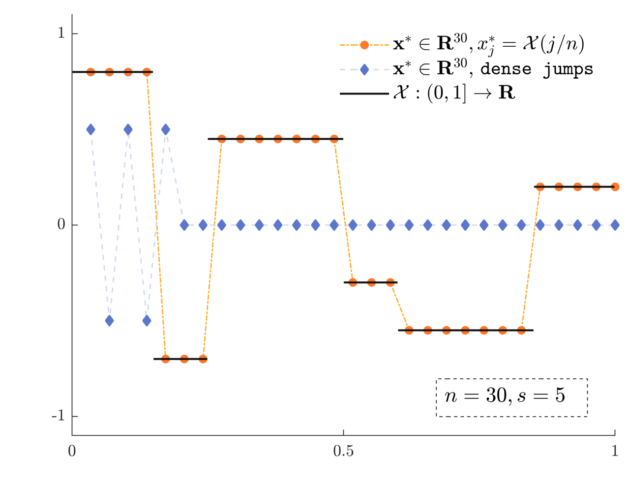
(a)

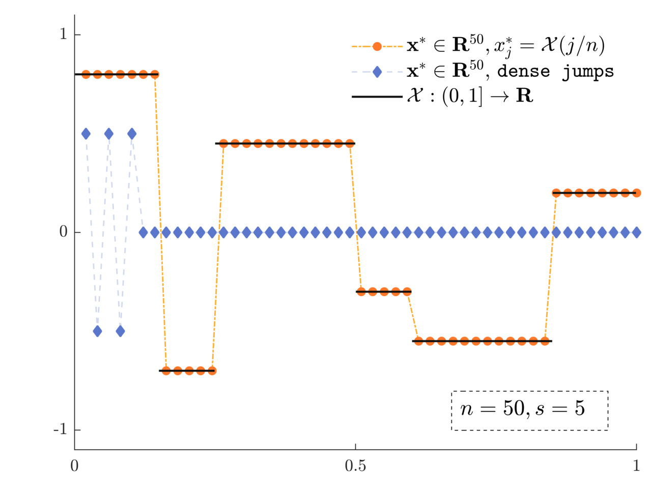
(b)

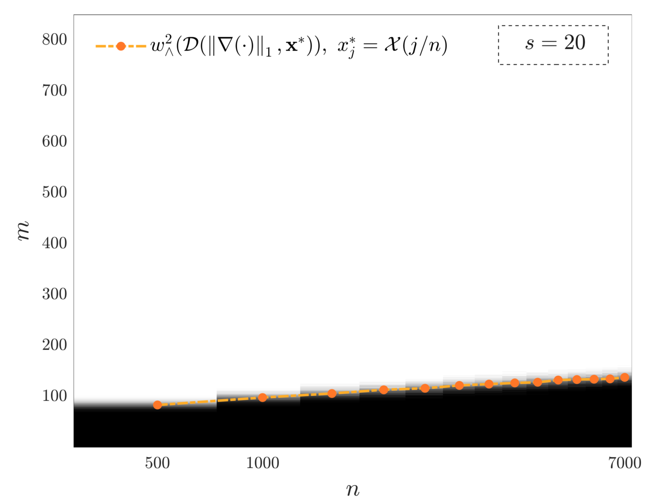
(c)

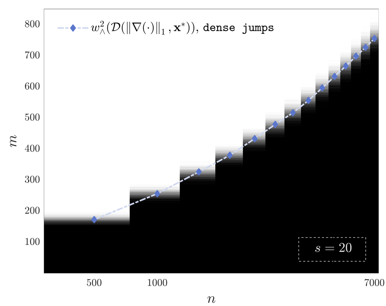
(d)

Figure 1: Numerical simulation. Subfigure 1(a) and 1(b) show schematic examples of the signal classes that are considered in this experiment at different resolution levels. The orange signal (with circle symbols) is defined as discretization of the piecewise constant function $\mathcal{X}\colon(0,1]\to\mathbb{R}$ with $s=5$ jump discontinuities that is plotted in black. The blue plot (with diamond symbols) shows a so-called dense-jump signal, which does not match the intuitive notion of a $5$-gradient-sparse signal; note that the spatial location of the jumps is chosen adaptively to the resolution level here, which does not correspond to a discretization of a piecewise constant function. For each signal class we have created phase transition plots: Subfigure 1(c) and 1(d) display the empirical probability of successful recovery via TV minimization (TV-1) for different pairs of ambient dimension $n$ and number of measurements $m$; note the horizontal axis uses a logarithmic scale. The corresponding grey tones reflect the observed probability of success, reaching from certain failure (black) to certain success (white). Additionally, we have estimated the conic Gaussian mean width of $\|\nabla(\cdot)\|_{1}$ at $\bm{x}^{\ast}$ (denoted by $w_{\wedge}^{2}(\mathcal{D}(\|\nabla(\cdot)\|_{1},\bm{x}^{\ast}))$), which is known to precisely capture the phase transition (cf. [ALMT14a]). The result of Subfigure 1(d) confirms that the class of dense-jump signals suffers from the $\sqrt{sn}$-bottleneck as predicted by [CX15a]. On the other hand, Subfigure 1(c) reveals that this bottleneck can be broken for discretized signals, as predicted by Theorem 3.2.

4 Discussion and Outlook

We have shown that the $\sqrt{sn}$-bottleneck for 1D TV recovery from Gaussian measurement can be broken for signals with well separated jump discontinuities. The results of Table 1 suggest that TV minimization in one spatial dimension plays a special role in this regard. However, we argue that such a phenomenon can also be observed in higher spatial dimensions. In fact, we conjecture that the common rate of $m\gtrsim s\cdot\operatorname{PolyLog}(n,s)$ only reflects worst-case scenarios, while it can be significantly improved for natural signal classes, such as piecewise constant functions with sufficiently smooth boundaries.

[sorting=nyt]

References

- [ALMT14] Dennis Amelunxen, Martin Lotz, Michael B. McCoy and Joel A. Tropp “Living on the edge: phase transitions in convex programs with random data” In Inf. Inference 3.3, 2014, pp. 224–294
- [BCNO11] A. Briani, A. Chambolle, M. Novaga and G. Orlandi “On the gradient flow of a one-homogeneous functional” In Confluentes Math. 03.04, 2011, pp. 617–635
- [CX15] Jian-Feng Cai and Weiyu Xu “Guarantees of total variation minimization for signal recovery” In Inf. Inference 4.4, 2015, pp. 328–353
- [CRT06] Emmanuel J. Candès, Justin K. Romberg and Terence Tao “Robust uncertainty principles: exact signal reconstruction from highly incomplete frequency information” In IEEE Trans. Inf. Theory 52.2, 2006, pp. 489–509
- [Cha04] Antonin Chambolle “An Algorithm for Total Variation Minimization and Applications” In J. Math. Imaging Vis. 20.1, 2004, pp. 89–97
- [CL97] Antonin Chambolle and Pierre-Louis Lions “Image recovery via total variation minimization and related problems” In Numer. Math. 76.2, 1997, pp. 167–188
- [Con13] L. Condat “A Direct Algorithm for 1-D Total Variation Denoising” In IEEE Signal Proc. Lett. 20.11, 2013, pp. 1054–1057
- [GMS20] M. Genzel, M. März and R. Seidel “Compressed Sensing with 1D Total Variation: Breaking Sample Complexity Barriers via Non-Uniform Recovery” Preprint arXiv:2001.09952, 2020
- [GKM20] Martin Genzel, Gitta Kutyniok and Maximilian März “-Analysis Minimization and Generalized (Co-)Sparsity: When Does Recovery Succeed?” In Appl. Comput. Harmon. Anal., 2020, pp. online\bibrangessepDOI: https://doi.org/10.1016/j.acha.2020.01.002
- [Gra07] Markus Grasmair “The Equivalence of the Taut String Algorithm and BV-Regularization” In J. Math. Imaging Vis. 27.1, 2007, pp. 59–66
- [KW14] F. Krahmer and R. Ward “Stable and Robust Sampling Strategies for Compressive Imaging” In IEEE Trans. Imag. Proc. 23.2, 2014, pp. 612–622
- [KKS17] Felix Krahmer, Christian Kruschel and Michael Sandbichler “Total Variation Minimization in Compressed Sensing” In Compressed Sensing and its Applications: Second International MATHEON Conference 2015 Birkhäuser, 2017, pp. 333–358
- [LJ10] M.. Little and N.. Jones “Sparse Bayesian step-filtering for high-throughput analysis of molecular machine dynamics” In IEEE International Conference on Acoustics, Speech, and Signal Processing (ICASSP 2010), 2010, pp. 4162–4165
- [LJ11] Max A. Little and Nick S. Jones “Generalized methods and solvers for noise removal from piecewise constant signals. I. Background theory” In Proc. Royal Soc. Lond. A 467.2135, 2011, pp. 3088–3114
- [MG97] Enno Mammen and Sara Geer “Locally Adaptive Regression Splines” In Ann. Statist. 25.1, 1997, pp. 387–413
- [NW13] D. Needell and R. Ward “Near-Optimal Compressed Sensing Guarantees for Total Variation Minimization” In IEEE Trans. Imag. Proc. 22.10, 2013, pp. 3941–3949
- [NW13a] Deanna. Needell and Rachel. Ward “Stable Image Reconstruction Using Total Variation Minimization” In SIAM J. Imag. Sci. 6.2, 2013, pp. 1035–1058
- [PF16] D. Perrone and P. Favaro “A Clearer Picture of Total Variation Blind Deconvolution” In IEEE Trans. Pattern Anal. Mach. Intell. 38.6, 2016, pp. 1041–1055
- [Poo15] Clarice. Poon “On the Role of Total Variation in Compressed Sensing” In SIAM J. Imag. Sci. 8.1, 2015, pp. 682–720
- [ROF92] Leonid I. Rudin, Stanley Osher and Emad Fatemi “Nonlinear total variation based noise removal algorithms” In Physica D: Nonlinear Phenomena 60.1–4, 1992, pp. 259–268
- [SKBBH15] M. Sandbichler, F. Krahmer, T. Berer, P. Burgholzer and M. Haltmeier “A Novel Compressed Sensing Scheme for Photoacoustic Tomography” In SIAM J. Appl. Math. 75.6, 2015, pp. 2475–2494
- [SPB15] I.. Selesnick, A. Parekh and İ. Bayram “Convex 1-D Total Variation Denoising with Non-convex Regularization” In IEEE Signal Process. Lett. 22.2, 2015, pp. 141–144
- [Sel12] Ivan W. Selesnick “Total variation denoising (an MM algorithm)”, Connexions, 2012
- [WWL14] Xiaopei Wu, Qingsi Wang and Mingyan Liu “In-situ Soil Moisture Sensing: Measurement Scheduling and Estimation Using Sparse Sampling” In ACM Trans. Sen. Netw. 11.2, 2014, pp. 26:1–26:29
- [ROF92a] Leonid I. Rudin, Stanley Osher and Emad Fatemi “Nonlinear total variation based noise removal algorithms” In Physica D: Nonlinear Phenomena 60.1–4, 1992, pp. 259–268
- [CL97a] Antonin Chambolle and Pierre-Louis Lions “Image recovery via total variation minimization and related problems” In Numer. Math. 76.2, 1997, pp. 167–188
- [MG97a] Enno Mammen and Sara Geer “Locally Adaptive Regression Splines” In Ann. Statist. 25.1, 1997, pp. 387–413
- [Cha04a] Antonin Chambolle “An Algorithm for Total Variation Minimization and Applications” In J. Math. Imaging Vis. 20.1, 2004, pp. 89–97
- [CRT06a] Emmanuel J. Candès, Justin K. Romberg and Terence Tao “Robust uncertainty principles: exact signal reconstruction from highly incomplete frequency information” In IEEE Trans. Inf. Theory 52.2, 2006, pp. 489–509
- [Gra07a] Markus Grasmair “The Equivalence of the Taut String Algorithm and BV-Regularization” In J. Math. Imaging Vis. 27.1, 2007, pp. 59–66
- [LJ10a] M.. Little and N.. Jones “Sparse Bayesian step-filtering for high-throughput analysis of molecular machine dynamics” In IEEE International Conference on Acoustics, Speech, and Signal Processing (ICASSP 2010), 2010, pp. 4162–4165
- [BCNO11a] A. Briani, A. Chambolle, M. Novaga and G. Orlandi “On the gradient flow of a one-homogeneous functional” In Confluentes Math. 03.04, 2011, pp. 617–635
- [LJ11a] Max A. Little and Nick S. Jones “Generalized methods and solvers for noise removal from piecewise constant signals. I. Background theory” In Proc. Royal Soc. Lond. A 467.2135, 2011, pp. 3088–3114
- [Sel12a] Ivan W. Selesnick “Total variation denoising (an MM algorithm)”, Connexions, 2012
- [Con13a] L. Condat “A Direct Algorithm for 1-D Total Variation Denoising” In IEEE Signal Proc. Lett. 20.11, 2013, pp. 1054–1057
- [NW13b] D. Needell and R. Ward “Near-Optimal Compressed Sensing Guarantees for Total Variation Minimization” In IEEE Trans. Imag. Proc. 22.10, 2013, pp. 3941–3949
- [NW13c] Deanna. Needell and Rachel. Ward “Stable Image Reconstruction Using Total Variation Minimization” In SIAM J. Imag. Sci. 6.2, 2013, pp. 1035–1058
- [ALMT14a] Dennis Amelunxen, Martin Lotz, Michael B. McCoy and Joel A. Tropp “Living on the edge: phase transitions in convex programs with random data” In Inf. Inference 3.3, 2014, pp. 224–294
- [KW14a] F. Krahmer and R. Ward “Stable and Robust Sampling Strategies for Compressive Imaging” In IEEE Trans. Imag. Proc. 23.2, 2014, pp. 612–622
- [WWL14a] Xiaopei Wu, Qingsi Wang and Mingyan Liu “In-situ Soil Moisture Sensing: Measurement Scheduling and Estimation Using Sparse Sampling” In ACM Trans. Sen. Netw. 11.2, 2014, pp. 26:1–26:29
- [CX15a] Jian-Feng Cai and Weiyu Xu “Guarantees of total variation minimization for signal recovery” In Inf. Inference 4.4, 2015, pp. 328–353
- [Poo15a] Clarice. Poon “On the Role of Total Variation in Compressed Sensing” In SIAM J. Imag. Sci. 8.1, 2015, pp. 682–720
- [SKBBH15a] M. Sandbichler, F. Krahmer, T. Berer, P. Burgholzer and M. Haltmeier “A Novel Compressed Sensing Scheme for Photoacoustic Tomography” In SIAM J. Appl. Math. 75.6, 2015, pp. 2475–2494
- [SPB15a] I.. Selesnick, A. Parekh and İ. Bayram “Convex 1-D Total Variation Denoising with Non-convex Regularization” In IEEE Signal Process. Lett. 22.2, 2015, pp. 141–144
- [PF16a] D. Perrone and P. Favaro “A Clearer Picture of Total Variation Blind Deconvolution” In IEEE Trans. Pattern Anal. Mach. Intell. 38.6, 2016, pp. 1041–1055
- [KKS17a] Felix Krahmer, Christian Kruschel and Michael Sandbichler “Total Variation Minimization in Compressed Sensing” In Compressed Sensing and its Applications: Second International MATHEON Conference 2015 Birkhäuser, 2017, pp. 333–358
- [GMS20a] M. Genzel, M. März and R. Seidel “Compressed Sensing with 1D Total Variation: Breaking Sample Complexity Barriers via Non-Uniform Recovery” Preprint arXiv:2001.09952, 2020
- [GKM20a] Martin Genzel, Gitta Kutyniok and Maximilian März “-Analysis Minimization and Generalized (Co-)Sparsity: When Does Recovery Succeed?” In Appl. Comput. Harmon. Anal., 2020, pp. online\bibrangessepDOI: https://doi.org/10.1016/j.acha.2020.01.002