Statistical analysis of edges and bredges
in configuration model networks

Abstract

A bredge (bridge-edge) in a network is an edge whose deletion would split the network component on which it resides into two separate components. Bredges are vulnerable links that play an important role in network collapse processes, which may result from node or link failures, attacks or epidemics. Therefore, the abundance and properties of bredges affect the resilience of the network to these collapse scenarios. We present analytical results for the statistical properties of bredges in configuration model networks. Using a generating function approach based on the cavity method, we calculate the probability $\widehat{P}(e\in{\rm B})$ that a random edge $e$ in a configuration model network with degree distribution $P(k)$ is a bredge (B). We also calculate the joint degree distribution $\widehat{P}(k,k^{\prime}|{\rm B})$ of the end-nodes $i$ and $i^{\prime}$ of a random bredge. We examine the distinct properties of bredges on the giant component (GC) and on the finite tree components (FC) of the network. On the finite components all the edges are bredges and there are no degree-degree correlations. We calculate the probability $\widehat{P}(e\in{\rm B}|{\rm GC})$ that a random edge on the giant component is a bredge. We also calculate the joint degree distribution $\widehat{P}(k,k^{\prime}|{\rm B},{\rm GC})$ of the end-nodes of bredges and the joint degree distribution $\widehat{P}(k,k^{\prime}|{\rm NB},{\rm GC})$ of the end-nodes of non-bredge (NB) edges on the giant component. Surprisingly, it is found that the degrees $k$ and $k^{\prime}$ of the end-nodes of bredges are correlated, while the degrees of the end-nodes of non-bredge edges are uncorrelated. We thus conclude that all the degree-degree correlations on the giant component are concentrated on the bredges. We calculate the covariance $\Gamma({\rm B},{\rm GC})$ of the joint degree distribution of end-nodes of bredges and show it is negative, namely bredges tend to connect high degree nodes to low degree nodes. We apply this analysis to ensembles of configuration model networks with degree distributions that follow a Poisson distribution (Erdős-Rényi networks), an exponential distribution and a power-law distribution (scale-free networks). The implications of these results are discussed in the context of common attack scenarios and network dismantling processes.

I Introduction

Network models provide a useful conceptual framework for the study of a large variety of systems and processes in science, technology and society Havlin2010 ; Newman2010 ; Estrada2011 ; Barrat2012 ; Latora2017 . These models consist of nodes and edges, where the nodes represent physical objects, while the edges represent the interactions between them. Unlike regular lattices in which all the nodes have the same coordination number, network models are characterized by a degree distribution $P(k)$. The backbone of a network often consists of high degree nodes or hubs, which connect the different branches and maintain the integrity of the network. In some applications, such as communication networks, it is crucial that the network will consist of a single connected component. However, mathematical models also produce networks that combine a giant component and isolated finite components, as well as fragmented networks that consist only of isolated finite components Bollobas2001 .

Networks are often exposed to the loss of nodes and edges, which may severely affect their functionality. Such losses may occur due to inadvertent node or edge failures, propagation of epidemics or deliberate attacks. Starting from a single connected component, as nodes or edges are deleted they may lead to the separation of network fragments from the giant component. As a result, the size of the giant component decreases until it completely disintegrates. The ultimate failure, when the network fragments into isolated finite components was studied extensively using percolation theory Albert2000 ; Cohen2000 ; Cohen2001 ; Schneider2011 .

A major factor in the sensitivity of networks to node or edge deletion processes is the fact that the deletion of a single node or a single edge may separate a whole fragment from the giant component. This fragmentation process greatly accelerates the disintegration of the network. Using iterative search algorithms one can identify the nodes whose deletion would break the component on which they reside into two or more components Hopcroft1973 ; Gibbons1985 ; Chaudhuri1998 Such nodes, called articulation points (APs), were recently studied in the context of network resilience and optimized attack strategies Tian2017 . Using similar methods one can also identify the edges whose deletion would break the component on which they reside into two separate components Tarjan1974 ; Italiano2012 . Such edges are called bridge-edges or cut-edges Bollobas1998 . Here we use the term bredges, which provides a shorthand for bridge-edges, and avoids a potential confusion with many other technical terms involving the word ‘bridge’. Moreover, the word ’bredge’ was used in ancient English as a synonym to the word ‘bridge’ Bredge1685 . In fact, an edge that does not participate in any cycle is a bredge (B). Thus, in network components that exhibit a tree structure, such as the finite tree components of configuration model networks, all the edges are bredges.

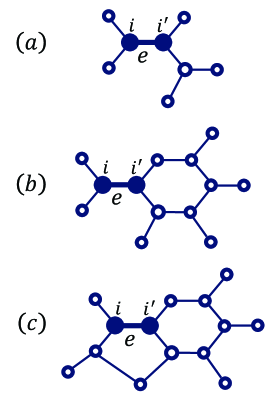
Figure 1: Schematic illustration of bredges and their surrounding network components: (a) A bredge $e$ (marked by a thick line) in a finite tree component. Deletion of the bredge $e$ would split the tree component into two separate tree components. The end-node $i$ will reside on one of the tree components and the end-node $i^{\prime}$ will reside on the other tree component; (b) A bredge $e$ (thick line) where one of its end nodes, $i^{\prime}$, resides on a cycle. Deletion of the bredge would split the network into two separate components; (c) Here the edge $e$, marked by a thick line, is not a bredge because the end nodes of this edge are connected by another path. As a result, upon deletion of the marked edge its two end nodes remain on the same network component.

In Fig. 1(a) we present a schematic illustration of a bredge $e$ (marked by a thick line) in a tree network and its end-nodes $i$ and $i^{\prime}$ (full circles). Deletion of the bredge would split the network into two separate tree components. In Fig. 1(b) we show a bredge $e$ (thick line), where one of its end-nodes, $i^{\prime}$, resides on a cycle. Deletion of the bredge would split the network into two separate components. The component that includes the end-node $i^{\prime}$ represents the giant component of the reduced network from which $e$ is removed, while the component that includes the end-node $i$ represents the finite tree component that is detached from the giant component upon deletion of $e$. The edge $e$ marked by a thick line in Fig. 1(c) is not a bredge because its end-nodes are connected by a path that does not go through $e$. As a result, upon deletion of $e$ its end-nodes $i$ and $i^{\prime}$ remain on the same network component. Since the paths connecting the end-nodes of an edge $e$ may be long, the determination of whether $e$ is a bredge or not cannot be done locally and requires access to the large-scale structure of the whole network Hopcroft1973 ; Gibbons1985 .

In practice, the functionality of most networks relies on the integrity of their giant components. Therefore, it is particularly important to study the properties of bredges and APs that reside on the giant component. These bredges and APs are vulnerable spots in the structure of a network, because the deletion of a single bredge may detach an entire tree branch from the giant component while the deletion of a single AP may detach one or several tree branches. This vulnerability is exploited in network attack strategies, which generate new bredges and AP via decycling processes and then attack them to dismantle the network Tian2017 ; Braunstein2016 ; Zdeborova2016 ; Wandelt2018 ; Ren2019 . While bredges and AP make the network vulnerable to attacks, they are advantageous in fighting epidemics. In particular, maintaining isolation between nodes connected by bredges prevents the spreading of epidemics between the network components connected by these bredges. Similarly, in communication networks the party in possession of an AP or a bredge may control, screen, block or alter the communication between the network components connected by the AP or the bredge.

There is an intricate connection between bredges and APs. On the one hand, each one of the end-nodes $i$ and $i^{\prime}$ of a bredge $e$ is either an AP (if its degree satisfies $k\geq 2$) or a leaf node (if its degree is $k=1$). On the other hand, if a node $i$ of degree $k\geq 2$ is an AP, then at least one of its $k$ edges must be a bredge. Moreover, in the case of a node $i$ of degree $k=2$, both edges of $i$ are bredges. The statistical properties of APs in configuration model networks were studied in a recent paper Tishby2018a . The probability $P(i\in{\rm AP})$ that a random node $i$ in a configuration model network with degree distribution $P(k)$ is an AP was calculated. Moreover, closed form expressions were obtained for the conditional probability $P(i\in{\rm AP}|k)$ that a random node of a given degree $k$ is an AP and for the conditional degree distribution $P(k|{\rm AP})$. An important property of an AP is the articulation rank $r$, which is the number of components that are added to the network upon deletion of the AP. For each node in the network the articulation rank satisfies $0\leq r\leq k$, where $k$ is the degree of the node. The articulation rank of a node which is not an AP is $r=0$, while the articulation ranks of APs satisfy $r\geq 1$. In fact, the articulation rank of an AP is the number of bredges connected to it. The distribution $P(r)$ of articulation ranks was calculated in Ref. Tishby2018a .

In this paper we present analytical results for the statistical properties of bredges in configuration model networks. In order to quantify the abundance of bredges, we calculate the probability $\widehat{P}(e\in{\rm B})$, that a random edge $e$ in a configuration model network with degree distribution $P(k)$ is a bredge. To characterize the statistical properties of bredges, we derive a closed form expression for the joint degree distribution $\widehat{P}(k,k^{\prime}|{\rm B})$ of the end-nodes $i$ and $i^{\prime}$ of a random bredge. We also examine the distinct properties of bredges on the giant component (GC) and on the finite tree components (FC) of the network. On the finite components all the edges are bredges, namely $\widehat{P}(e\in{\rm B}|{\rm FC})=1$. We calculate the probability $\widehat{P}(e\in{\rm B}|{\rm GC})$ that a random edge that resides on the giant component is a bredge and the joint degree distribution $\widehat{P}(k,k^{\prime}|{\rm B},{\rm GC})$ between the end-nodes of bredges on the giant component. It is found that the degrees $k$ and $k^{\prime}$ of the end-nodes of a bredge that resides on the giant component are correlated. This is in contrast to the end-nodes of random edges in the network and to the end-nodes of non-bredge (NB) edges on the giant component, which exhibit no degree-degree correlations. We thus conclude that all the degree-degree correlations on the giant component are concentrated on the bredges. We calculate the covariance $\Gamma({\rm B},{\rm GC})$ and show that it is negative, which means that bredges on the giant component tend to connect high degree nodes to low degree nodes. We apply these results to ensembles of configuration model networks with degree distributions that follow a Poisson distribution (Erdős-Rényi networks), an exponential distribution and a power-law distribution (scale-free networks).

The paper is organized as follows. In Sec. II we describe the configuration model network and its construction. In Sec. III we present the generating functions of the degree distribution. In Sec. IV we present a statistical analysis of nodes on the giant component and on the finite components. In Sec. V we present a statistical analysis of edges on the giant and finite components. In Sec. VI we present a detailed statistical analysis of bredges. In Sec. VII we apply these results to configuration model networks with a Poisson degree distribution (ER networks), exponential degree distribution and power-law degree distribution (scale-free networks). The results are discussed in Sec. VIII and summarized in Sec. IX.

II The configuration model

The configuration model is an ensemble of uncorrelated random networks whose degree sequences are drawn from a given degree distribution $P(k)$. The first moment (mean degree) and the second moment of $P(k)$ are denoted by $\langle K^{n}\rangle$, where $n=1$ and $2$, respectively, while the variance is given by ${\mathbb{V}}[K]=\langle K^{2}\rangle-\langle K\rangle^{2}$. The support of the degree distribution of random networks is often bounded from below by $k_{\rm min}\geq 1$ such that $P(k)=0$ for $0\leq k\leq k_{\rm min}-1$, with non-zero values of $P(k)$ only for $k\geq k_{\rm min}$. For example, the commonly used choice of $k_{\rm min}=1$ eliminates the possibility of isolated nodes in the network. Choosing $k_{\rm min}=2$ also eliminates the leaf nodes. One may also control the upper bound by imposing $k\leq k_{\rm max}$. This may be important in the case of finite networks with heavy-tail degree distributions such as power-law distributions. The configuration model network ensemble is a maximum entropy ensemble under the condition that the degree distribution $P(k)$ is imposed Molloy1995 ; Molloy1998 ; Newman2001 . Here we focus on the case of undirected networks.

To generate a network instance drawn from an ensemble of configuration model networks of $N$ nodes, with a given degree distribution $P(k)$, one draws the degrees of the $N$ nodes independently from $P(k)$. This gives rise to a degree sequence of the form $k_{1},k_{2},\dots,k_{N}$. For the discussion below it is convenient to list the degree sequence in a decreasing order of the form $k_{1}\geq k_{2}\geq\dots\geq k_{N}$. It turns out that not every possible degree sequence is graphic, namely admissible as a degree sequence of a network. Therefore, before trying to construct a network with a given degree sequence, one should first confirm the graphicality of the degree sequence. To be graphic, a degree sequence must satisfy two conditions. The first condition is that the sum of the degrees is an even number, namely $\sum_{i}k_{i}=2L$, where $L$ is an integer that represents the number of edges in the network. The second condition is expressed by the Erdős-Gallai theorem, which states that an ordered sequence of the form $k_{1}\geq k_{2}\geq\dots\geq k_{N}$ that satisfies the first condition is graphic if and only if the condition

$$\sum_{i=1}^{n}k_{i}\leq n(n-1)+\sum_{i=n+1}^{N}\min(k_{i},n)$$ (1)

holds for all values of $n$ in the range $1\leq n\leq N-1$ Erdos1960b ; Choudum1986 .

A convenient way to construct a configuration model network is to prepare the $N$ nodes such that each node $i$ is connected to $k_{i}$ half edges or stubs Newman2010 . At each step of the construction, one connects a random pair of stubs that belong to two different nodes $i$ and $j$ that are not already connected, forming an edge between them. This procedure is repeated until all the stubs are exhausted. The process may get stuck before completion in case that all the remaining stubs belong to the same node or to pairs of nodes that are already connected. In such case one needs to perform some random reconnections in order to complete the construction.

In the dense-network limit, configuration model networks consist of a single connected component, while in the dilute-network limit they consist of many finite tree components. At intermediate densities they exhibit a coexistence between a giant component, which is extensive in the network size, and many non-extensive finite tree components. Some commonly studied configuration model networks can be described in terms of single parameter families of degree distributions. A particularly convenient choice of the parameter is the mean degree $c=\langle K\rangle$. In this case, the degree distribution can be expressed by $P(k)=P_{c}(k)$, such that small values of $c$ correspond to the dilute network limit while large values of $c$ correspond to the dense network limit. At some value $c_{0}$, referred to as the percolation threshold, there is a percolation transition below which the network consists of finite tree components and above which a giant component emerges. The percolation transition is a second order phase transition, whose order parameter is the fraction $g$ of nodes that reside on the giant component. Below the transition, where $c<c_{0}$, the order parameter is $g=0$, while for $c>c_{0}$ the function $g=g(c)$ gradually increases.

III The generating functions of the degree distribution

Consider a configuration model network with a given degree distribution $P(k)$. To obtain the probability $g$ that a random node in the network belongs to the giant component, one needs to first calculate the probability $\tilde{g}$, that a node $i$ selected via a random edge $e$ belongs to the giant component of the reduced network, from which the edge $e$ is removed. The probability $\tilde{g}$ is determined by Havlin2010 ; Newman2010

$$1-{\tilde{g}}=G_{1}(1-{\tilde{g}}),$$ (2)

where

$$G_{1}(x)=\sum_{k=1}^{\infty}x^{k-1}{\widetilde{P}}(k)$$ (3)

is the generating function of the distribution

$${\widetilde{P}}(k)=\frac{k}{\langle K\rangle}P(k),$$ (4)

which is the degree distribution of nodes that are sampled via random edges. The solution of Eq. (2) is an attractive fixed point (Sec. 13.8 in Ref. Newman2010 ). Using $\tilde{g}$, one can then obtain the probability $g$ from the equation

$$g=1-G_{0}(1-{\tilde{g}}),$$ (5)

where

$$G_{0}(x)=\sum_{k=0}^{\infty}x^{k}P(k)$$ (6)

is the generating function of the degree distribution $P(k)$. The two generating functions are related to each other by $G_{1}(x)=G^{\prime}_{0}(x)/G^{\prime}_{0}(1)$, where $G^{\prime}_{0}(x)$ is the derivative of $G_{0}(x)$.

From the definitions of $G_{0}(x)$ and $G_{1}(x)$ in Eqs. (6) and (3), respectively, we find that $0<G_{0}(x),G_{1}(x)<1$ for $0<x<1$ and $G_{0}(1)=G_{1}(1)=1$ This means that $x=1$ is a fixed point for both generating functions. Therefore, $g=\tilde{g}=0$ is a solution of Eqs. (2) and (5). This solution corresponds to the case of subcritical networks, in which there is no giant component. In some networks there are no isolated nodes (of degree $k=0$) and no leaf nodes (of degree $k=1$). In such networks $P(0)=0$ and $P(1)=0$, while $P(k)>0$ only for $k\geq 2$. The generating functions associated with these networks satisfy $G_{0}(0)=0$ and $G_{1}(0)=0$. This implies that in such networks both $x=0$ and $x=1$ are fixed points of both $G_{0}(x)$ and $G_{1}(x)$ and there are no other fixed points with $0<x<1$. The coexistence of a giant component and non-trivial finite tree components (that consist of more than a single node) appears only in case that the degree distributions $P(k)$ supports a non-trivial solution of Eq. (2), in which $0<\tilde{g}<1$. This requires a non-zero probability of leaf-nodes, namely $P(1)>0$, and thus occurs only when $k_{\rm min}=0$ or $k_{\rm min}=1$. In large configuration model networks in which $k_{\rm min}\geq 2$ and the mean degree satisfies the condition $c>2$, the giant component encompasses the whole network and $g=\tilde{g}=1$ Bonneau2017 .

Here we focus on configuration model networks with degree distributions $P(k)$, which are bounded from below by $k_{\rm min}=0$ or $1$. Under suitable conditions, such networks may exhibit a coexistence between a giant component and finite tree components. The condition for the existence of a giant component can be expressed in the form

$$\frac{\langle K^{2}\rangle}{\langle K\rangle}-1>1,$$ (7)

which is known as the Molloy-Reed criterion Molloy1995 ; Molloy1998 . In order to discuss this condition, consider a node $i$ that is sampled via a random edge $e$. The excess degree $k_{\rm ex}$ of $i$ is the number of other edges apart from the edge $e$, namely $k_{\rm ex}=k-1$, where $k$ is the degree of $i$. In essence, the condition of Eq. (7) states that a giant component exists if the expectation value of the excess degree of nodes sampled via a random edge exceeds $1$. Thus, the percolation threshold $c_{0}$ is the value of the mean degree $\langle K\rangle$ at which $\langle K^{2}\rangle=2\langle K\rangle$.

IV Statistical analysis of nodes

Below we analyze the statistical properties of randomly sampled nodes in configuration model networks. We calculate the probability that a random node resides on the giant component (and the complementary probability that it resides on one of the finite components). We also analyze the distinct statistical properties of the nodes that reside on the giant component and on the finite components.

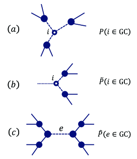
Figure 2: (a) A random node $i$ (empty circle) of degree $k$ in a configuration model network (left). The probability that $i$ does not reside on the giant component is equal to the probability that none of its $k$ neighbors (full circles) resides on the giant component of the reduced network (right) from which $i$ is removed, together with its links (dashed lines). (b) A node $i$ (empty circle) of degree $k$ sampled via a random edge (left), which is marked as a dashed line. We are interested in the probability that $i$ does not reside on the giant component of the reduced network from which the sampled edge (dashed line) is removed. This probability is equal to the probability that none of its $k-1$ remaining neighbors of $i$ resides on the giant component of the further reduced network (right) from which the node $i$ is removed together with its links (dashed lines). (c) A random edge $e$ with end-nodes $i$ and $i^{\prime}$ of degrees $k$ and $k^{\prime}$, respectively (left). The probability that $e$ does not reside on the giant component is equal to the probability that none of its two end-nodes resides on the giant component of the reduced network from which $e$ is removed. This probability is equal to the probability that none of the $k-1$ remaining neighbors of $i$ and none of the $k^{\prime}-1$ remaining neighbors of $i^{\prime}$ resides on the giant component of the further reduced network (right) from which $i$ and $i^{\prime}$ are removed together with their links (dashed lines).

IV.1 The fraction of nodes that reside on the giant/finite components

The probability that a random node $i$ in a configuration model network resides on the giant component is Tishby2018b ; Tishby2019

$$P(i\in{\rm GC})=g,$$ (8)

where $g$ is given by Eq. (5), while the probability that it resides on one of the finite components is

$$P(i\in{\rm FC})=1-g.$$ (9)

A node $i$ of a given degree $k$ resides on the giant component if at least one of its $k$ neighbors resides on the giant component of the reduced network from which $i$ is removed [Fig. 2(a)]. Using the theoretical framework of the cavity method Mezard1985 ; Mezard2003 ; Mezard2009 ; Ferraro2015 , each neighbor of $i$ can be considered as a node selected via a random edge. Therefore, the probability that each one of the neighbors of $i$ resides on the giant component of the reduced network from which $i$ is removed is given by $\tilde{g}$. Moreover, due to the locally tree-like structure of configuration model networks, the probabilities of different neighbors of $i$ to reside on the giant component of the reduced network from which $i$ is removed are independent of each other. Therefore, the probability that a node $i$ selected randomly from all the nodes of degree $k$ in the network resides on the giant component, is given by Tishby2018b ; Tishby2019

$$P(i\in{\rm GC}|k)=1-(1-\tilde{g})^{k},$$ (10)

where $\tilde{g}$ is given by Eq. (2), while the probability that it resides on one of the finite tree components is given by

$$P(i\in{\rm FC}|k)=(1-\tilde{g})^{k}.$$ (11)

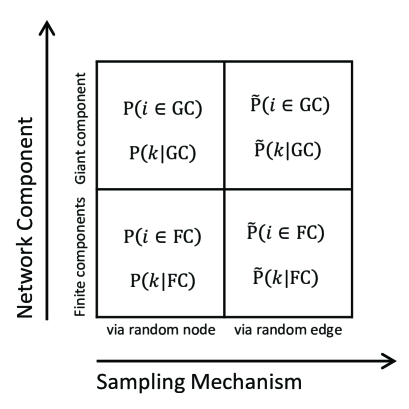
Figure 3: Illustration of the four categories of nodes considered in this paper, presented in the form of a two by two matrix diagram. The horizontal axis accounts for the two sampling procedures, namely random node sampling and node sampling via random edges. The vertical axis accounts for the location of a node in the network, which can be either on the giant component or on one of the finite tree components. Each one of the four categories of nodes exhibits different statistical properties.

Clearly, the probability of $i$ to reside on the giant component is an increasing function of the degree $k$, while the probability of $i$ to reside on one of the finite components is a decreasing function of $k$.

The different categories of nodes in configuration model networks, in terms of the sampling procedure and their location in the network, are illustrated in Fig. 3 in the form of a two by two matrix diagram. The horizontal axis accounts for the two sampling procedures, namely random node sampling and node sampling via random edges. The vertical axis accounts for the location of a node in the network, which can be either on the giant component or on one of the finite tree components. Each one of the four categories of nodes exhibits different statistical properties. Such $2\times 2$ matrix diagrams are used extensively in the analysis of decision making processes and business management Lowy2004 .

IV.2 The degree distributions of nodes on the giant/finite components

The micro-structure of the giant component of configuration model networks was recently studied Tishby2018b ; Tishby2019 . It was shown that the degree distribution, conditioned on the giant component, is given by

$$P(k|{\rm GC})=\frac{1-(1-\tilde{g})^{k}}{g}P(k),$$ (12)

while the degree distribution conditioned on the finite components is given by

$$P(k|{\rm FC})=\frac{(1-\tilde{g})^{k}}{1-g}P(k),$$ (13)

where $k\geq k_{\rm min}$. In the analysis below we focus on degree distributions whose support is bounded from below by either $k_{\rm min}=0$ or $k_{\rm min}=1$, which enable the coexistence between the giant component and the finite tree components. The derivations apply to both cases. The specific value of $k_{\rm min}$ is not specified in each equation, but it is implicitly assumed that in the case of $k_{\rm min}=1$ the probability $P(0)=0$.

As expected, Eq. (12) satisfies $P(0|{\rm GC})=0$ even for $k_{\rm min}=0$, namely there are no isolated nodes on the giant component. Isolated nodes are considered as finite tree components of size $s=1$. The probability that a random node on the finite components is an isolated node is given by $P(0|{\rm FC})=P(0)/(1-g)$, namely the fraction of isolated nodes on the finite components is higher than in the whole network. Regarding leaf nodes of degree $k=1$, their fraction on the giant component, given by $P(1|{\rm GC})=(\tilde{g}/g)P(1)$, is higher than in the whole network in case that $g<\tilde{g}$ and lower in case that $g>\tilde{g}$. Since $g>\tilde{g}[1-P(0)]$ the former case may occur only in networks that include isolated nodes, in which $P(0)>0$ Tishby2018a . Since in the coexistence phase, where $0<g,\tilde{g}<1$, the probabilities $g$ and $\tilde{g}$ satisfy the condition Tishby2018a

$$\frac{(1-\tilde{g})^{2}}{1-g}<1,$$ (14)

the fraction of nodes of degrees $k\geq 2$ on the finite tree components is lower than in the whole network. The condition of Eq. (14) can also be expressed in the form

$$\frac{(2-\tilde{g})\tilde{g}}{g}>1.$$ (15)

Note that the numerator on the left hand side of Eq. (15) satisfies

$$(2-\tilde{g})\tilde{g}<1.$$ (16)

To show this we define $\tilde{h}=1-\tilde{g}$ and obtain $(2-\tilde{g})\tilde{g}=1-\tilde{h}^{2}<1$. The degree distribution of the whole network is recovered by

$$P(k)=P(k|{\rm GC})P(i\in{\rm GC})+P(k|{\rm FC})P(i\in{\rm FC}),$$ (17)

where $P(i\in{\rm GC})$ and $P(i\in{\rm FC})$ are given by Eqs. (8) and (9), respectively.

The giant component of a configuration model network consists of a 2-core which is decorated by tree branches. The 2-core (2-CORE) is a connected component, such that each node on the 2-core has links to at least two other nodes that reside on the 2-core Seidman1983 ; Dorogovtsev2006a ; Dorogovtsev2006b ; Yuan2016 . Moreover, each node on the 2-core of a configuration model network resides on at least one cycle. The nodes on the tree branches belong to the 1-core of the giant component but not to the 2-core. This is expressed by $i\in{\rm GC}\cap\overline{\mbox{2-CORE}}$, where $\overline{X}$ represents the complementary set of $X$ and $X\cap Y$ is the intersection of $X$ and $Y$. The degree distribution of the nodes on the 2-core of the giant component is given by

$$P(k|\mbox{2-CORE})=\frac{1-(1-\tilde{g})^{k}-k\tilde{g}(1-\tilde{g})^{k-1}}{g-\tilde{g}(1-\tilde{g})\langle K\rangle}P(k),$$ (18)

while the degree distribution of the nodes on the tree branches of the giant component is given by

$$P(k|{\rm GC}\cap\overline{\mbox{2-CORE}})=(1-\tilde{g})^{k-2}\widetilde{P}(k).$$ (19)

The probability that a random node on the giant component resides on the 2-core is given by

$$P(i\in\mbox{2-CORE}|{\rm GC})=1-\frac{\tilde{g}(1-\tilde{g})}{g}\langle K\rangle,$$ (20)

while the probability that it resides on one of the tree branches is given by

$$P(i\in\overline{\mbox{2-CORE}}|{\rm GC})=\frac{\tilde{g}(1-\tilde{g})}{g}\langle K\rangle.$$ (21)

IV.3 The mean degrees of nodes on the giant/finite components

The mean degree of the nodes that reside on the giant component is given by $\mathbb{E}[K|{\rm GC}]=\sum_{k}kP(k|{\rm GC})$. Inserting $P(k|{\rm GC})$ from Eq. (12) and carrying out the summation, we obtain

$$\mathbb{E}[K|{\rm GC}]=\frac{(2-\tilde{g})\tilde{g}}{g}\langle K\rangle.$$ (22)

Using Eq. (15) we conclude that $\mathbb{E}[K|{\rm GC}]>\langle K\rangle$, namely the mean degree of the nodes that reside on the giant component is larger than the mean degree of the whole network.

The mean degree of the nodes that reside on the finite tree components is denoted by $\mathbb{E}[K|{\rm FC}]$. Using $P(k|{\rm FC})$ from Eq. (13), we obtain

$$\mathbb{E}[K|{\rm FC}]=\frac{(1-\tilde{g})^{2}}{1-g}\langle K\rangle.$$ (23)

Using Eq. (14) we conclude that the mean degree of the nodes that reside on the finite tree components is smaller than the mean degree of the whole network, namely $\mathbb{E}[k|{\rm FC}]<\langle K\rangle$. The mean degree of the whole network is recovered by

$$\langle K\rangle={\mathbb{E}}[K|{\rm GC}]P(i\in{\rm GC})+{\mathbb{E}}[K|{\rm FC}]P(i\in{\rm FC}),$$ (24)

where $P(i\in{\rm GC})$ and $P(i\in{\rm FC})$ are given by Eqs. (8) and (9), respectively.

IV.4 The variance of the degree distributions on the giant/finite components

The second moment of the degree distribution $P(k|{\rm GC})$ of the nodes that reside on the giant component is given by

$$\mathbb{E}[K^{2}|{\rm GC}]=\frac{1}{g}\biggl{\{}\langle K^{2}\rangle-(1-\tilde{g})^{2}\big{[}1+G^{\prime}_{1}(1-\tilde{g})\big{]}\langle K\rangle\biggr{\}},$$ (25)

where $G^{\prime}_{1}(x)$ is the derivative of $G_{1}(x)$. Since the fixed point of Eq. (2) is a stable fixed point, the derivative satisfies $G^{\prime}_{1}(1-\tilde{g})<1$. Writing $G^{\prime}_{1}(1-\tilde{g})$ explicitly, in the form

$$G^{\prime}_{1}(1-\tilde{g})=\frac{1}{\langle K\rangle}\sum_{k=2}^{\infty}k(k-1)(1-\tilde{g})^{k-2}P(k),$$ (26)

we find that it satisfies

$$G^{\prime}_{1}(1-\tilde{g})<\min\left\{\frac{\langle K^{2}\rangle}{\langle K\rangle}-1,1\right\}.$$ (27)

Inserting this result into Eq. (25) and using Eq. (15), it is found that in the coexistence phase, where $0<g,\tilde{g}<1$, $\mathbb{E}[K^{2}|{\rm GC}]>\langle K^{2}\rangle$. In the dilute network regime of $0<\tilde{g}\ll 1$, just above the percolation transition, one can expand the right hand side of Eq. (26) to first order in $\tilde{g}$ and obtain

$$G^{\prime}_{1}(1-\tilde{g})\simeq\frac{\langle K^{2}\rangle}{\langle K\rangle}-1-\left(\frac{\langle K^{3}\rangle}{\langle K\rangle}-3\frac{\langle K^{2}\rangle}{\langle K\rangle}+2\right)\tilde{g}+\mathcal{O}\left(\tilde{g}^{2}\right).$$ (28)

The variance of $P(k|{\rm GC})$ is given by

$${\mathbb{V}}[K|{\rm GC}] = \frac{1}{g}\biggl{\{}\langle K^{2}\rangle-(1-\tilde{g})^{2}\big{[}1+G^{\prime}_{1}(1-\tilde{g})\big{]}\langle K\rangle\biggr{\}}$$ (29)

$$-\frac{[(2-\tilde{g})\tilde{g}]^{2}}{g^{2}}\langle K\rangle^{2}.$$

While both the first and second moments of $P(k|{\rm GC})$ are larger than the corresponding moments of $P(k)$, the variance ${\mathbb{V}}[K|{\rm GC}]$ may be either larger or smaller than ${\mathbb{V}}[K]$, depending on the specific properties of the degree distribution.

The second moment of the degree distribution $P(k|{\rm FC})$ of the nodes that reside on the finite tree components is denoted by $\mathbb{E}[K^{2}|{\rm FC}]$. Using $P(k|{\rm FC})$ from Eq. (13), we obtain

$$\mathbb{E}[K^{2}|{\rm FC}]=\frac{(1-\tilde{g})^{2}}{1-g}\left[1+G^{\prime}_{1}(1-\tilde{g})\right]\langle K\rangle.$$ (30)

Using Eqs. (14) and (27) one can show that $\mathbb{E}[K^{2}|{\rm FC}]<\langle K^{2}\rangle$. The variance of $P(k|{\rm FC})$ is denoted by ${\mathbb{V}}[K|{\rm FC}]$. Using the first and second moments from Eqs. (23) and (30), respectively, we obtain

$${\mathbb{V}}[K|{\rm FC}]=\frac{(1-\tilde{g})^{2}}{1-g}\langle K\rangle\left\{1+G^{\prime}_{1}(1-\tilde{g})-\frac{(1-\tilde{g})^{2}}{1-g}\langle K\rangle\right\}.$$ (31)

While both the first and second moments of $P(k|{\rm FC})$ are smaller than the corresponding moments of $P(k)$, the variance ${\mathbb{V}}[K|{\rm FC}]$ may be either larger or smaller than ${\mathbb{V}}[K]$, depending on the specific properties of the degree distribution.

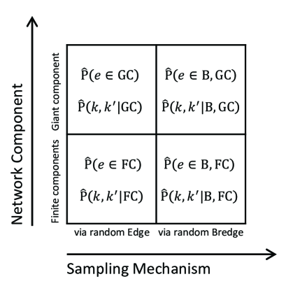
Figure 4: Illustration of the four categories of edges considered in this paper, presented in the form of a two by two matrix diagram. The horizontal axis accounts for the two sampling procedures, namely random sampling from all the edges in the network or random sampling restricted to those edges which are bredges. The vertical axis accounts for the location of an edge in the network, which can be either on the giant component or in one of the finite tree components. Each one of the four categories of edges exhibits different statistical properties.

V Statistical analysis of edges

Below we analyze the statistical properties of randomly selected edges in configuration model networks. We calculate the probability that a random edge resides on the giant component (and the complementary probability that it resides on one of the finite components). We also analyze the distinct statistical properties of the edges that reside on the giant component and of those that reside on the finite components.

The different categories of edges in terms of the sampling procedure and their location in the network are illustrated in Fig. 4. The horizontal axis accounts for the two sampling procedures, namely random sampling from all the edges in the network or random sampling restricted to those edges which are bredges. The vertical axis accounts for the location of an edge in the network, which can be either on the giant component or in one of the finite tree components. Each one of the four categories of edges exhibits different statistical properties.

V.1 The fraction of edges that reside on the giant/finite components

Consider a randomly chosen end-node $i$ of a random edge $e$ [Fig. 2(b)]. The probability that $i$ resides on the giant component of the reduced network from which $e$ is removed is

$$\widetilde{P}(i\in{\rm GC})=\tilde{g},$$ (32)

where $\tilde{g}$ is given by Eq. (2), while the probability that $i$ resides on one of the finite components of the reduced network is

$$\widetilde{P}(i\in{\rm FC})=1-\tilde{g}.$$ (33)

Consider a random edge $e$ [Fig. 2(c)]. The probability that $e$ resides on one of the finite tree components of the network amounts to the probability that both its end-nodes reside on finite components of the reduced network from which $e$ is removed. It is thus given by

$$\widehat{P}(e\in{\rm FC})=(1-\tilde{g})^{2}.$$ (34)

Therefore, the complementary probability that a random edge $e$ resides on the giant component is

$$\widehat{P}(e\in{\rm GC})=(2-\tilde{g})\tilde{g}.$$ (35)

The degrees of end-nodes satisfy $k\geq 1$ even in case that $k_{\rm min}=0$. The probability that the end-node $i$ belongs to the giant component of the reduced network from which $e$ is removed, is given by

$$\widetilde{P}(i\in{\rm GC}|k)=1-(1-\tilde{g})^{k-1},$$ (36)

while the probability that it belongs to one of the finite components of the reduced network is

$$\widetilde{P}(i\in{\rm FC}|k)=(1-\tilde{g})^{k-1},$$ (37)

where $k\geq 1$.

Consider a random edge $e$ whose end-nodes $i$ and $i^{\prime}$ are of degrees $k\geq 1$ and $k^{\prime}\geq 1$, respectively. The probability that such an edge resides on the giant component is given by

$$\widehat{P}(e\in{\rm GC|k,k^{\prime}})=1-(1-\tilde{g})^{k+k^{\prime}-2},$$ (38)

while the probability that it resides on one of the finite tree components is

$$\widehat{P}(e\in{\rm FC|k,k^{\prime}})=(1-\tilde{g})^{k+k^{\prime}-2}.$$ (39)

Interestingly, these probabilities depend only on the sum of $k$ and $k^{\prime}$ rather than on each one of them separately. For $k=k^{\prime}=1$ one obtains $\widehat{P}(e\in{\rm GC|1,1})=0$ and $\widehat{P}(e\in{\rm FC|1,1})=1$. This is due to the fact that in this case $i$ and $i^{\prime}$ form a dimer, which is isolated from the rest of the network. As the sum $k+k^{\prime}$ increases, the probability that the edge $e$ resides on one of the finite components decays exponentially while the probability that it resides on the giant component converges towards $1$.

V.2 The marginal degree distributions of end-nodes

The degree distribution of the end-nodes of random edges is given by Eq. (4), where $k\geq 1$. The degree distribution of the end-nodes of random edges that reside on the giant component is given by

$$\widetilde{P}(k|{\rm GC})=\frac{k}{\mathbb{E}[K|{\rm GC}]}P(k|{\rm GC}).$$ (40)

Inserting $P(k|{\rm GC})$ from Eq. (12) and $\mathbb{E}[K|{\rm GC}]$ from Eq. (22), we obtain

$$\widetilde{P}(k|{\rm GC})=\frac{1-(1-\tilde{g})^{k}}{(2-\tilde{g})\tilde{g}}\widetilde{P}(k),$$ (41)

where $k\geq 1$. From Eq. (41) one finds that the fraction of end-nodes of degree $k=1$ on the giant component, given by $\widetilde{P}(1|{\rm GC})=\widetilde{P}(1)/(2-\tilde{g})$, is lower than in the whole network. Interestingly, the fraction of end-nodes of degree $k=2$ on the giant component, given by $\widetilde{P}(2|{\rm GC})=\widetilde{P}(2)$, is identical to their fraction in the whole network. For $k\geq 3$ it is found that $\widetilde{P}(k|{\rm GC})>\widetilde{P}(k)$, namely nodes of degrees $k\geq 3$ are more probable on the giant component compared to the whole network. In the limit of $k\rightarrow\infty$ $\widetilde{P}(k|{\rm GC})\rightarrow\widetilde{P}(k)/[(2-\tilde{g})\tilde{g}]$, where $(2-\tilde{g})\tilde{g}<1$ [Eq. (16)]. The degree distribution of the end-nodes of random edges that reside on the finite components is given by

$$\widetilde{P}(k|{\rm FC})=\frac{k}{\mathbb{E}[K|{\rm FC}]}P(k|{\rm FC}).$$ (42)

Inserting $P(k|{\rm FC})$ from Eq. (13) and $\mathbb{E}[K|{\rm FC}]$ from Eq. (23), we obtain

$$\widetilde{P}(k|{\rm FC})=(1-\tilde{g})^{k-2}\widetilde{P}(k),$$ (43)

where $k\geq 1$. The degree distribution $\widetilde{P}(k)$ of the end-nodes of random edges in the network is recovered by

$$\widetilde{P}(k)=\widetilde{P}(k|{\rm GC})\widehat{P}(e\in{\rm GC})+\widetilde{P}(k|{\rm FC})\widehat{P}(e\in{\rm FC}),$$ (44)

where $\widetilde{P}(k|{\rm GC})$ is given by Eq. (41), $\widetilde{P}(k|{\rm FC})$ is given by Eq. (43), $\widehat{P}(e\in{\rm GC})$ is given by Eq. (35) and $\widehat{P}(e\in{\rm FC})$ is given by Eq. (34).

From Eq. (43) one finds that the fraction of end-nodes of degree $k=1$ on the finite components, given by $\widetilde{P}(1|{\rm FC})=\widetilde{P}(1)/(1-\tilde{g})$, is higher than in the whole network. The fraction of end-nodes of degree $k=2$ on the finite components is identical to their fraction in the whole network. For any value of $k\geq 3$ the fraction of end-nodes of degree $k$ on the finite components is lower than in the whole network. The ’phase separation’ between the giant component and the finite components may thus be considered as a distillation process, in which high-degree nodes tend to concentrate on the giant component while low-degree nodes end up in the finite components.

V.3 The mean degrees of end-nodes

The mean degree of end-nodes of random edges is denoted by $\widetilde{\mathbb{E}}[K]$. Using $\widetilde{P}(k)$ from Eq. (4), we obtain

$$\widetilde{\mathbb{E}}[K]=\frac{\langle K^{2}\rangle}{\langle K\rangle}.$$ (45)

The mean degree of end-nodes of random edges that reside on the finite tree components is denoted by $\widetilde{\mathbb{E}}[K|{\rm FC}]$. Using $\widetilde{P}(k|{\rm FC})$ from Eq. (43), we obtain

$$\widetilde{\mathbb{E}}[K|{\rm FC}]=1+G_{1}^{\prime}(1-\tilde{g}),$$ (46)

where $G^{\prime}_{1}(x)$ is the derivative of $G_{1}(x)$. Interestingly, this implies that $G_{1}^{\prime}(1-\tilde{g})$ can be interpreted as the mean excess degree $\widetilde{\mathbb{E}}[K_{\rm ex}|{\rm FC}]=\widetilde{\mathbb{E}}[K|{\rm FC}]-1$ of end-nodes of edges that reside on the finite components. In general, the mean excess degree of nodes sampled via random edges is analogous to the basic reproduction ratio $R_{0}$ of infectious diseases Diekmann2000 and to the neutron multiplication factor of nuclear chain reactions Duderstadt1976 . Using Eq. (27) it is found that $\widetilde{\mathbb{E}}[K|{\rm FC}]<\widetilde{\mathbb{E}}[K]$.

The mean degree of end-nodes of random edges that reside on the giant component is denoted by $\widetilde{\mathbb{E}}[K|{\rm GC}]$. Using $\widetilde{P}(k|{\rm GC})$ from Eq. (41), we obtain

$$\widetilde{\mathbb{E}}[K|{\rm GC}]=\frac{1}{(2-\tilde{g})\tilde{g}}\left\{\frac{\langle K^{2}\rangle}{\langle K\rangle}-(1-\tilde{g})^{2}[1+G_{1}^{\prime}(1-\tilde{g})]\right\}.$$ (47)

Using Eq. (27) it is found that $\widetilde{\mathbb{E}}[K|{\rm GC}]>\widetilde{\mathbb{E}}[K]$. Note that in heavy tail degree distributions the mean degree $\widetilde{\mathbb{E}}[K|{\rm GC}]$ of the end-nodes that reside on the giant component may diverge even under conditions in which $\langle K\rangle$ is finite. This is due to the fact that in such distributions the second moment $\langle K^{2}\rangle$ that appears on the right hand side of Eq. (47) may diverge, leading to the divergence of $\widetilde{\mathbb{E}}[K|{\rm GC}]$. The mean degree $\widetilde{\mathbb{E}}[K]$ can be recovered by

$$\widetilde{\mathbb{E}}[K]=\widetilde{\mathbb{E}}[K|{\rm GC}]\widehat{P}(e\in{\rm GC})+\widetilde{\mathbb{E}}[K|{\rm FC}]\widehat{P}(e\in{\rm FC}).$$ (48)

V.4 The variance of the degree distribution of end-nodes

The second moment of the degree distribution $\widetilde{P}(k)$ of the end-nodes of random edges is denoted by $\widetilde{\mathbb{E}}[K^{2}]$. Using $\widetilde{P}(k)$ from Eq. (4), we obtain

$$\widetilde{\mathbb{E}}[K^{2}]=\frac{\langle K^{3}\rangle}{\langle K\rangle}.$$ (49)

The variance of $\widetilde{P}(k)$ is denoted by $\widetilde{\mathbb{V}}[K]$. Using the first moment $\widetilde{\mathbb{E}}[K]$ from Eq. (45) and the second moment $\widetilde{\mathbb{E}}[K^{2}]$ from Eq. (49), we obtain

$$\widetilde{\mathbb{V}}[K]=\frac{\langle K^{3}\rangle}{\langle K\rangle}-\frac{\langle K^{2}\rangle^{2}}{\langle K\rangle^{2}}.$$ (50)

The second moment of the degree distribution $\widetilde{P}(k|{\rm FC})$ of end-nodes of random edges that reside on the finite tree components is denoted by $\widetilde{\mathbb{E}}[K^{2}|{\rm FC}]$. Using $\widetilde{P}(k|{\rm FC})$ from Eq. (43), we obtain

$$\widetilde{\mathbb{E}}[K^{2}|{\rm FC}]=(1-\tilde{g})G^{\prime\prime}_{1}(1-\tilde{g})+3G_{1}^{\prime}(1-\tilde{g})+1,$$ (51)

where $G^{\prime\prime}_{1}(x)$ is the second derivative of $G_{1}(x)$. Writing $G^{\prime\prime}_{1}(1-\tilde{g})$ explicitly in the form

$$G^{\prime\prime}_{1}(1-\tilde{g})=\frac{1}{\langle K\rangle}\sum_{k=3}^{\infty}k(k-1)(k-2)(1-\tilde{g})^{k-3}P(k),$$ (52)

we find that it satisfies

$$G^{\prime\prime}_{1}(1-\tilde{g})\leq\frac{\langle K^{3}\rangle}{\langle K\rangle}-3\frac{\langle K^{2}\rangle}{\langle K\rangle}+2,$$ (53)

where equality is obtained for $\tilde{g}=0$. Combining this result with Eq. (27), it is found that in the coexistence phase, where $0<g,\tilde{g}<1$, the second moment satisfies $\widetilde{\mathbb{E}}[K^{2}|{\rm FC}]<\widetilde{\mathbb{E}}[K^{2}]$. In the dilute network regime of $0<\tilde{g}\ll 1$, just above the percolation transition, one can expand the right hand side of Eq. (52) to first order in $\tilde{g}$ and obtain

$$G^{\prime\prime}_{1}(1-\tilde{g}) \simeq \frac{\langle K^{3}\rangle}{\langle K\rangle}-3\frac{\langle K^{2}\rangle}{\langle K\rangle}+2-\Bigg{(}\frac{\langle K^{4}\rangle}{\langle K\rangle}-6\frac{\langle K^{3}\rangle}{\langle K\rangle}$$ (54)

$$+11\frac{\langle K^{2}\rangle}{\langle K\rangle}-6\Bigg{)}\tilde{g}+\mathcal{O}\left(\tilde{g}^{2}\right).$$

Using Eq. (53) it is found that $\widetilde{\mathbb{E}}[K^{2}|{\rm FC}]<\widetilde{\mathbb{E}}[K^{2}]$.

The variance of the degree distribution $\widetilde{P}(k|{\rm FC})$ of the end-nodes that reside on the finite components is denoted by $\widetilde{\mathbb{V}}[K|{\rm FC}]$. Using the first and second moments from Eqs. (46) and (51), respectively, we obtain

$$\widetilde{\mathbb{V}}[K|{\rm FC}]=(1-\tilde{g})G^{\prime\prime}_{1}(1-\tilde{g})+G_{1}^{\prime}(1-\tilde{g})\big{[}1-G_{1}^{\prime}(1-\tilde{g})\big{]}.$$ (55)

While both the first and second moments of $\widetilde{P}(k|{\rm FC})$ are smaller than the corresponding moments of $\widetilde{P}(k)$, the variance $\widetilde{{\mathbb{V}}}[K|{\rm FC}]$ may be either larger or smaller than $\widetilde{{\mathbb{V}}}[K]$, depending on the specific properties of the degree distribution.

The second moment of the degree distribution $\widetilde{P}(k|{\rm GC})$ of the end-nodes that reside on the giant component is denoted by $\widetilde{\mathbb{E}}[K^{2}|{\rm GC}]$. Using $\widetilde{P}(k|{\rm GC})$ from Eq. (41), we obtain

$$\widetilde{\mathbb{E}}[K^{2}|{\rm GC}] = \frac{1}{(2-\tilde{g})\tilde{g}}\Bigg{\{}\frac{\langle K^{3}\rangle}{\langle K\rangle}-(1-\tilde{g})^{2}\big{[}(1-\tilde{g})$$ (56)

$$\times G^{\prime\prime}_{1}(1-\tilde{g})+3G_{1}^{\prime}(1-\tilde{g})+1\big{]}\Bigg{\}}.$$

Using Eq. (53) it is found that $\widetilde{\mathbb{E}}[K^{2}|{\rm GC}]>\widetilde{\mathbb{E}}[K^{2}]$. The variance of the degree distribution $\widetilde{P}(k|{\rm GC})$ of the end-nodes that reside on the giant component is denoted by $\widetilde{\mathbb{V}}[K|{\rm GC}]$. Using the first and second moments from Eqs. (47) and (56), respectively, we obtain

$$\widetilde{\mathbb{V}}[K|{\rm GC}] = \frac{1}{(2-\tilde{g})\tilde{g}}\Bigg{\{}\frac{\langle K^{3}\rangle}{\langle K\rangle}-(1-\tilde{g})^{2}\big{[}(1-\tilde{g})$$

$$\times G^{\prime\prime}_{1}(1-\tilde{g})+3G_{1}^{\prime}(1-\tilde{g})+1\big{]}\Bigg{\}}$$

$$- \frac{1}{[(2-\tilde{g})\tilde{g}]^{2}}\left\{\frac{\langle K^{2}\rangle}{\langle K\rangle}-(1-\tilde{g})\big{[}1+G_{1}^{\prime}(1-\tilde{g})\big{]}\right\}^{2}.$$

While both the first and second moments of $\widetilde{P}(k|{\rm GC})$ are larger than the corresponding moments of $\widetilde{P}(k)$, the variance $\widetilde{{\mathbb{V}}}[K|{\rm GC}]$ may be either larger or smaller than $\widetilde{{\mathbb{V}}}[K]$, depending on the specific properties of the degree distribution. The variance $\widetilde{\mathbb{V}}[K|{\rm GC}]$ is used below as a normalization factor for the covariance of the joint degree distribution of edges that reside on the giant component, which yields the Pearson correlation coefficient.

V.5 The joint degree distribution of end-nodes

The joint degree distribution $\widehat{P}(k,k^{\prime})$ of the end-nodes $i$ and $i^{\prime}$ of a random edge in a configuration model network with degree distribution $P(k)$ is given by

$$\widehat{P}(k,k^{\prime})=\widetilde{P}(k)\widetilde{P}(k^{\prime}),$$ (58)

where $\widetilde{P}(k)$ is given by Eq. (4). Note that in Eq. (58) the degrees satisfy $k,k^{\prime}\geq 1$. The end-nodes $i$ and $i^{\prime}$ are considered as two distinguishable objects. Thus, $\widehat{P}(k,k^{\prime})$ is the probability that $i$ is of degree $k$ and $i^{\prime}$ is of degree $k^{\prime}$. The probability that $i$ is of degree $k^{\prime}$ and $i^{\prime}$ is of degree $k$ is given by $\widehat{P}(k^{\prime},k)=\widehat{P}(k,k^{\prime})$. Therefore, the probabilities $\widehat{P}(k,k^{\prime})$, $k,k^{\prime}\geq 1$ constitute a symmetric matrix.

Under conditions that were specified above, configuration model networks exhibit a coexistence of a giant component and finite tree components. The set of finite tree components constitute a subnetwork which is itself a configuration model network, and is in the subcritical regime Bollobas2001 ; Katzav2018 . Since there are no degree-degree correlations on the finite components, the joint degree distribution of pairs of end-nodes of random edges that reside on the finite components is given by

$$\widehat{P}(k,k^{\prime}|{\rm FC})=\widetilde{P}(k|{\rm FC})\widetilde{P}(k^{\prime}|{\rm FC}),$$ (59)

where $k,k^{\prime}\geq 1$. Inserting $\widetilde{P}(k|{\rm FC})$ from Eq. (43) into Eq. (59) we obtain

$$\widehat{P}(k,k^{\prime}|{\rm FC})=(1-\tilde{g})^{k+k^{\prime}-4}\widetilde{P}(k)\widetilde{P}(k^{\prime}).$$ (60)

The joint degree distribution $\widehat{P}(k,k^{\prime})$ can be expressed as a weighted sum of the joint degree distribution of end-nodes of edges that reside on the giant component and on the finite components in the form

$$\widehat{P}(k,k^{\prime})=\widehat{P}(k,k^{\prime}|{\rm GC})\widehat{P}(e\in{\rm GC})+\widehat{P}(k,k^{\prime}|{\rm FC})\widehat{P}(e\in{\rm FC}),$$ (61)

where $\widehat{P}(e\in{\rm GC})$ and $\widehat{P}(e\in{\rm FC})$ are given by Eqs. (35) and (34), respectively. Extracting $\widehat{P}(k,k^{\prime}|{\rm GC})$ from Eq. (61), we obtain

$$\widehat{P}(k,k^{\prime}|{\rm GC})=\frac{\widehat{P}(k,k^{\prime})-\widehat{P}(k,k^{\prime}|{\rm FC})\widehat{P}(e\in{\rm FC})}{\widehat{P}(e\in{\rm GC})}.$$ (62)

Note that nodes that reside on the giant component satisfy $k,k^{\prime}\geq 1$. Moreover, the giant component does not include edges for which $k=k^{\prime}=1$ (dimers), thus $\widehat{P}(1,1|{\rm GC})=0$. As a result, the lowest possible degrees of the end-nodes of an edge that resides on the giant component are $(k,k^{\prime})=(1,2)$ or $(k,k^{\prime})=(2,1)$. This condition can be expressed in the form $k+k^{\prime}\geq 3$, in addition to $k,k^{\prime}\geq 1$. Inserting the joint degree distributions $\widehat{P}(k,k^{\prime})$ and $\widehat{P}(k,k^{\prime}|{\rm FC})$ from Eqs. (58) and (60), respectively, and the probabilities $\widehat{P}(e\in{\rm FC})$ and $\widehat{P}(e\in{\rm GC})$ from Eqs. (34) and (35), respectively, into Eq. (62), we obtain

$$\widehat{P}(k,k^{\prime}|{\rm GC})=\frac{1-(1-\tilde{g})^{k+k^{\prime}-2}}{(2-\tilde{g})\tilde{g}}\widetilde{P}(k)\widetilde{P}(k^{\prime}),$$ (63)

where $k,k^{\prime}\geq 1$ and $k+k^{\prime}\geq 3$. Extracting $\widetilde{P}(k)$ from Eq. (41), we obtain

$$\widetilde{P}(k)=\frac{(2-\tilde{g})\tilde{g}}{1-(1-\tilde{g})^{k}}\widetilde{P}(k|{\rm GC}).$$ (64)

Inserting $\widetilde{P}(k)$ and $\widetilde{P}(k^{\prime})$ from Eq. (64) into Eq. (63), we obtain

$$\widehat{P}(k,k^{\prime}|{\rm GC}) = (2-\tilde{g})\tilde{g}\frac{1-(1-\tilde{g})^{k+k^{\prime}-2}}{[1-(1-\tilde{g})^{k}][1-(1-\tilde{g})^{k^{\prime}}]}$$ (65)

$$\times\widetilde{P}(k|{\rm GC})\widetilde{P}(k^{\prime}|{\rm GC}).$$

Inserting $k=k^{\prime}=1$ into Eq. (65), we confirm that $\widehat{P}(1,1|{\rm GC})=0$. In the opposite limit of $k,k^{\prime}\rightarrow\infty$, it is found that $\widehat{P}(k,k^{\prime}|{\rm GC})\rightarrow(2-\tilde{g})\tilde{g}\widetilde{P}(k|{\rm GC})\widetilde{P}(k^{\prime}|{\rm GC})$. Since $(2-\tilde{g})\tilde{g}<1$, the probability that both end-nodes of an edge that resides on the giant component will be of high degree is suppressed. We thus conclude that the degree-degree correlations between end-nodes of random edges on the giant component are negative, namely the giant component is disassortative Newman2002b ; Newman2003a ; Newman2003b ; Johnson2010 ; Mizutaka2018 .

V.6 The covariance of the joint degree distribution of end-nodes of edges

The covariance of the joint degree distribution of end-nodes of edges in a configuration model network is denoted by

$$\Gamma=\widehat{\mathbb{E}}[KK^{\prime}]-\widetilde{\mathbb{E}}[K]\ \widetilde{\mathbb{E}}[K^{\prime}],$$ (66)

where

$$\widehat{\mathbb{E}}[KK^{\prime}]=\sum_{k=1}^{\infty}\sum_{k^{\prime}=1}^{\infty}kk^{\prime}\widehat{P}(k,k^{\prime}),$$ (67)

is the mixed second moment of $\widehat{P}(k,k^{\prime})$. In configuration model networks there are no degree-degree correlations and therefore $\Gamma=0$. Moreover, the sub-network that consists of all the finite tree components is also a configuration model network. Therefore, the covariance of the joint degree distribution of end-nodes of edges that reside on the finite tree components satisfies $\Gamma({\rm FC})=0$.

The covariance of the joint degree distribution of end-nodes of edges that reside on the giant component is given by

$$\Gamma({\rm GC})=\widehat{\mathbb{E}}[KK^{\prime}|{\rm GC}]-\widetilde{\mathbb{E}}[K|{\rm GC}]\ \widetilde{\mathbb{E}}[K^{\prime}|{\rm GC}],$$ (68)

where

$$\widehat{\mathbb{E}}[KK^{\prime}|{\rm GC}]=\sum_{k=1}^{\infty}\sum_{k^{\prime}=1}^{\infty}kk^{\prime}\widehat{P}(k,k^{\prime}|{\rm GC})$$ (69)

is the mixed second moment of $\widehat{P}(k,k^{\prime}|{\rm GC})$ and the mean degree $\widetilde{\mathbb{E}}[K|{\rm GC}]$ is given by Eq. (47). Inserting $\widehat{P}(k,k^{\prime}|{\rm GC})$ from Eq. (63) into Eq. (69), carrying out the summations, and inserting the result into Eq. (68), we obtain

$$\Gamma({\rm GC})=-\frac{(1-\tilde{g})^{2}}{[(2-\tilde{g})\tilde{g}]^{2}}\left[\frac{\langle K^{2}\rangle}{\langle K\rangle}-1-G^{\prime}_{1}(1-\tilde{g})\right]^{2}.$$ (70)

It is found that $\Gamma({\rm GC})<0$, namely the giant component of a configuration model network is always disassortative Newman2002b ; Newman2003a ; Newman2003b ; Johnson2010 ; Mizutaka2018 . This means that on the giant component high degree nodes tend to connect to low degree nodes and vice versa.

In the dilute network regime of $0<\tilde{g}\ll 1$, just above the percolation transition, the giant component is small but it exhibits strong degree-degree correlations. Using Eq. (28), it is found that in this regime

$$\Gamma({\rm GC})\simeq-\frac{1}{4}\left(\frac{\langle K^{3}\rangle}{\langle K\rangle}-3\frac{\langle K^{2}\rangle}{\langle K\rangle}+2\right)^{2}+\mathcal{O}\left(\tilde{g}^{2}\right).$$ (71)

In the opposite limit of $\tilde{g}\rightarrow 1^{-}$, in which the giant component expands to encompass the whole network (apart from any isolated nodes), $\Gamma({\rm GC})\rightarrow 0$. More precisely, in the regime of $1-\tilde{g}\ll 1$ the covariance of the joint degree distribution of end-nodes on the giant component decays according to $\Gamma({\rm GC})\sim-(1-\tilde{g})^{2}$. The Pearson correlation coefficient for pairs of end-nodes of edges that reside on the giant component is given by

$$R({\rm GC})=\frac{\Gamma({\rm GC})}{\widetilde{\mathbb{V}}[K|{\rm GC}]},$$ (72)

where $\widetilde{\mathbb{V}}[K|{\rm GC}]$ is given by Eq. (LABEL:eq:tVKGC). Unlike the covariance $\Gamma({\rm GC})$, the Pearson correlation coefficient is bounded in the range $-1\leq R({\rm GC})\leq 1$. It is thus a more suitable measure for the comparison of the correlations between the degrees of pairs of end-nodes in different populations of edges and bredges.

VI Statistical analysis of bredges

VI.1 The probability that a random edge is a bredge

Consider a random edge $e$ in a configuration model network of $N$ nodes with degree distribution $P(k)$. The probability $\widehat{P}(e\in{\rm B})$ that $e$ is a bredge is given by Wu2018

$$\widehat{P}(e\in{\rm B})=1-\tilde{g}^{2},$$ (73)

where $\tilde{g}$ is given by Eq. (2). This is due to the fact that in order that a random edge will not be a bredge, its end-nodes $i$ and $i^{\prime}$ should both belong to the giant component of the reduced network from which the edge $e$ was removed. The probability for each one of these nodes to belong to the giant component of the reduced network is $\tilde{g}$. Thus, the probability that both of them belong to the giant component of the reduced network is $\tilde{g}^{2}$. The probability that at least one of them does not belong to the giant component of the reduced network is thus $1-\tilde{g}^{2}$, which leads to Eq. (73). The complementary probability, that a random edge $e$ is a non-bredge (NB) edge is given by $\widehat{P}(e\in{\rm NB})=\tilde{g}^{2}$. Therefore, in the dilute network regime of $0<\tilde{g}\ll 1$, just above the percolation transition, almost every edge is a bredge.

Consider a random edge $e$ whose end-nodes $i$ and $i^{\prime}$ are of known degrees, $k$ and $k^{\prime}$, where $k,k^{\prime}\geq 1$. In order that the edge $e$ will not be a bredge, both $i$ and $i^{\prime}$ should reside on the giant component of the reduced network from which $e$ is removed. Therefore, the probability that $e$ is a bredge is given by

$$\widehat{P}(e\in{\rm B}|k,k^{\prime})=1-[1-(1-\tilde{g})^{k-1}][1-(1-\tilde{g})^{k^{\prime}-1}],$$ (74)

where $k,k^{\prime}\geq 1$. This result can also be expressed in the form

$$\widehat{P}(e\in{\rm B}|k,k^{\prime})=(1-\tilde{g})^{k-1}+(1-\tilde{g})^{k^{\prime}-1}-(1-\tilde{g})^{k+k^{\prime}-2}.$$ (75)

The probability $\widehat{P}(e\in{\rm B})$ that a random edge is a bredge can be expressed in the form

$$\widehat{P}(e\in{\rm B})=\sum_{k,k^{\prime}=1}^{\infty}\widehat{P}(e\in{\rm B}|k,k^{\prime})\widehat{P}(k,k^{\prime}).$$ (76)

Inserting the conditional probability $\widehat{P}(e\in{\rm B}|k,k^{\prime})$ from Eq. (75) into Eq. (76) and carrying out the summation, one recovers Eq. (73).

The probability $\widehat{P}(e\in{\rm B})$ can be expressed as a sum of two terms, where one term accounts for nodes that reside on the giant component and the other accounts for nodes that reside on the finite components. It takes the form

$$\widehat{P}(e\in{\rm B})=\widehat{P}(e\in{\rm B}|{\rm GC})\widehat{P}(e\in{\rm GC})+\widehat{P}(e\in{\rm B}|{\rm FC})\widehat{P}(e\in{\rm FC}).$$ (77)

Extracting the conditional probability $\widehat{P}(e\in{\rm B}|{\rm GC})$ that a random edge on the giant component is a bredge, one obtains

$$\widehat{P}(e\in{\rm B}|{\rm GC})=\frac{\widehat{P}(e\in{\rm B})-\widehat{P}(e\in{\rm B}|{\rm FC})\widehat{P}(e\in{\rm FC})}{\widehat{P}(e\in{\rm GC})}.$$ (78)

Since all the edges on the finite tree components are bredges, $\widehat{P}(e\in{\rm B}|{\rm FC})=1$. Inserting $\widehat{P}(e\in{\rm B})$ from Eq. (73), $\widehat{P}(e\in{\rm GC})$ from Eq. (35) and $\widehat{P}(e\in{\rm FC})$ from Eq. (34) into Eq. (78), we obtain

$$\widehat{P}(e\in{\rm B}|{\rm GC})=\frac{2(1-\tilde{g})}{2-\tilde{g}}.$$ (79)

Therefore, the complementary probability that a random edge on the giant component is not a bredge is given by

$$\widehat{P}(e\in{\rm NB}|{\rm GC})=\frac{\tilde{g}}{2-\tilde{g}}.$$ (80)

To calculate the fraction of bredges that belong to the giant component one can use Bayes’ theorem, and obtain

$$\widehat{P}(e\in{\rm GC}|{\rm B})=\frac{\widehat{P}(e\in{\rm B}|{\rm GC})\widehat{P}(e\in{\rm GC})}{\widehat{P}(e\in{\rm B})}.$$ (81)

Inserting $\widehat{P}(e\in{\rm B}|{\rm GC})$ from Eq. (79), $\widehat{P}(e\in{\rm GC})$ from Eq. (35) and $\widehat{P}(e\in{\rm B})$ from Eq. (73) into Eq. (81), we obtain

$$\widehat{P}(e\in{\rm GC}|{\rm B})=\frac{2\tilde{g}}{1+\tilde{g}}.$$ (82)

Therefore, the fraction of bredges that reside on the finite components is

$$\widehat{P}(e\in{\rm FC}|{\rm B})=\frac{1-\tilde{g}}{1+\tilde{g}}.$$ (83)

The conditional probability $P(e\in{\rm B}|k,k^{\prime})$, given by Eq. (75), can be expressed as a sum of two terms, where one term accounts for nodes that reside on the giant component and the other accounts for nodes that reside on the finite components. It takes the form

$$\widehat{P}(e\in{\rm B}|k,k^{\prime}) = \widehat{P}(e\in{\rm B}|{\rm GC},k,k^{\prime})\widehat{P}(e\in{\rm GC}|k,k^{\prime})$$ (84)

$$+ \widehat{P}(e\in{\rm B}|{\rm FC},k,k^{\prime})\widehat{P}(e\in{\rm FC}|k,k^{\prime}).$$

The conditional probability $\widehat{P}(e\in{\rm GC}|k,k^{\prime})$, given by Eq. (38), takes non-zero values only for degrees $k,k^{\prime}\geq 1$ whose sum satisfies $k+k^{\prime}\geq 3$, while $\widehat{P}(e\in{\rm FC}|k,k^{\prime})$ is given by Eq. (39), where $k,k^{\prime}\geq 1$. Since all the edges that reside on the finite components are bredges, $\widehat{P}(e\in{\rm B}|{\rm FC},k,k^{\prime})=1$. Extracting the conditional probability $\widehat{P}(e\in{\rm B}|{\rm GC},k,k^{\prime})$ from Eq. (84), one obtains

$$\widehat{P}(e\in{\rm B}|{\rm GC},k,k^{\prime})=\frac{\widehat{P}(e\in{\rm B}|k,k^{\prime})-\widehat{P}(e\in{\rm B}|{\rm FC},k,k^{\prime})\widehat{P}(e\in{\rm FC}|k,k^{\prime})}{\widehat{P}(e\in{\rm GC}|k,k^{\prime})}.$$ (85)

Since all the edges on the finite tree components are bredges, $\widehat{P}(e\in{\rm B}|{\rm FC},k,k^{\prime})=1$, where $k,k^{\prime}\geq 1$. Evaluating the right hand side of Eq. (85), we obtain

$$\widehat{P}(e\in{\rm B}|{\rm GC},k,k^{\prime})=\frac{(1-\tilde{g})^{k-1}+(1-\tilde{g})^{k^{\prime}-1}-2(1-\tilde{g})^{k+k^{\prime}-2}}{1-(1-\tilde{g})^{k+k^{\prime}-2}},$$ (86)

where $k,k^{\prime}\geq 1$ and $k+k^{\prime}\geq 3$. The probability that an edge connecting end-nodes of degrees $k$ and $k^{\prime}$ on the giant component is not a bredge is thus given by

$$\widehat{P}(e\in{\rm NB}|{\rm GC},k,k^{\prime})=\frac{1-(1-\tilde{g})^{k-1}-(1-\tilde{g})^{k^{\prime}-1}+(1-\tilde{g})^{k+k^{\prime}-2}}{1-(1-\tilde{g})^{k+k^{\prime}-2}},$$ (87)

where $k,k^{\prime}\geq 1$ and $k+k^{\prime}\geq 3$.

VI.2 The joint degree distribution of the end-nodes of bredges

The joint degree distribution of the nodes on both sides of a bredge can be expressed in the form

$$\widehat{P}(k,k^{\prime}|{\rm B})=\frac{\widehat{P}(e\in{\rm B}|k,k^{\prime})\widehat{P}(k,k^{\prime})}{\widehat{P}(e\in{\rm B})}.$$ (88)

Inserting $\widehat{P}(e\in{\rm B}|k,k^{\prime})$ from Eq. (75), $\widehat{P}(k,k^{\prime})$ from Eq. (58) and $\widehat{P}(e\in{\rm B})$ from Eq. (73) into Eq. (88), we obtain

$$\widehat{P}(k,k^{\prime}|{\rm B})=\frac{1}{1+\tilde{g}}\left[(1-\tilde{g})^{k-2}+(1-\tilde{g})^{k^{\prime}-2}-(1-\tilde{g})^{k+k^{\prime}-3}\right]\widetilde{P}(k)\widetilde{P}(k^{\prime}),$$ (89)

where $k,k^{\prime}\geq 1$. Below we consider the joint degree distributions $\widehat{P}(k,k^{\prime}|{\rm B},{\rm GC})$ and $\widehat{P}(k,k^{\prime}|{\rm B},{\rm FC})$ of the end-nodes of random bredges on the giant component and on the finite components, respectively. Since all the edges on the finite components are bredges, the joint degree distribution of the end nodes of random bredges that reside on the finite components satisfies $\widehat{P}(k,k^{\prime}|{\rm B},{\rm FC})=\widehat{P}(k,k^{\prime}|{\rm FC})$, where $\widehat{P}(k,k^{\prime}|{\rm FC})$ is given by Eq. (60).

The conditional probability $\widehat{P}(k,k^{\prime}|{\rm B})$ can be expressed in the form

$$\widehat{P}(k,k^{\prime}|{\rm B}) = \widehat{P}(k,k^{\prime}|{\rm B},{\rm GC})\widehat{P}(e\in{\rm GC}|{\rm B})$$ (90)

$$+ \widehat{P}(k,k^{\prime}|{\rm B},{\rm FC})\widehat{P}(e\in{\rm FC}|{\rm B}).$$

Extracting $\widehat{P}(k,k^{\prime}|{\rm B},{\rm GC})$ from Eq. (90) we obtain

$$\widehat{P}(k,k^{\prime}|{\rm B},{\rm GC})=\frac{\widehat{P}(k,k^{\prime}|{\rm B})-\widehat{P}(k,k^{\prime}|{\rm B},{\rm FC})\widehat{P}(e\in{\rm FC}|{\rm B})}{\widehat{P}(e\in{\rm GC}|{\rm B})}.$$ (91)

Inserting $\widehat{P}(e\in{\rm FC}|{\rm B})$ from Eq. (83) and $\widehat{P}(e\in{\rm GC}|{\rm B})$ from Eq. (79) into Eq. (92), we obtain

$$\widehat{P}(k,k^{\prime}|{\rm B},{\rm GC})=\frac{1}{2\tilde{g}}\left[(1-\tilde{g})^{k-2}+(1-\tilde{g})^{k^{\prime}-2}-2(1-\tilde{g})^{k+k^{\prime}-3}\right]\widetilde{P}(k)\widetilde{P}(k^{\prime}),$$ (92)

where $k,k^{\prime}\geq 1$ and $k+k^{\prime}\geq 3$.

The joint degree distribution of pairs of end-nodes of random edges on the giant component can be decomposed in the form

$$\widehat{P}(k,k^{\prime}|{\rm GC})=\widehat{P}(k,k^{\prime}|{\rm B},{\rm GC})\widehat{P}(e\in{\rm B}|{\rm GC})+\widehat{P}(k,k^{\prime}|{\rm NB},{\rm GC})\widehat{P}(e\in{\rm NB}|{\rm GC}),$$ (93)

where the first term on the right hand side accounts for the bredges and the second term account for all the edges that are not bredges. Note that the joint degree distribution $\widehat{P}(k,k^{\prime}|{\rm NB},{\rm GC})$ may take non-zero values only under conditions in which both $k\geq 2$ and $k^{\prime}\geq 2$. Extracting the joint degree distribution on the edges that are not bredges, we obtain

$$\widehat{P}(k,k^{\prime}|{\rm NB},{\rm GC})=\frac{\widehat{P}(k,k^{\prime}|{\rm GC})-\widehat{P}(k,k^{\prime}|{\rm B},{\rm GC})\widehat{P}(e\in{\rm B}|{\rm GC})}{\widehat{P}(e\in{\rm NB}|{\rm GC})}.$$ (94)

Inserting $\widehat{P}(k,k^{\prime}|{\rm GC})$ from Eq. (63), $\widehat{P}(k,k^{\prime}|{\rm B},{\rm GC})$ from Eq. (92), $\widehat{P}(e\in{\rm B}|{\rm GC})$ from Eq. (79) and $\widehat{P}(e\in{\rm NB}|{\rm GC})$ from Eq. (80), we obtain

$$\widehat{P}(k,k^{\prime}|{\rm NB},{\rm GC})=\frac{1}{\tilde{g}^{2}}\left[1-(1-\tilde{g})^{k-1}-(1-\tilde{g})^{k^{\prime}-1}+(1-\tilde{g})^{k+k^{\prime}-2}\right]\widetilde{P}(k)\widetilde{P}(k^{\prime}),$$ (95)

where $k,k^{\prime}\geq 2$. Eq. (95) can be written as a product of the form

$$\widehat{P}(k,k^{\prime}|{\rm NB},{\rm GC})=\left[\frac{1-(1-\tilde{g})^{k-1}}{\tilde{g}}\right]\widetilde{P}(k)\left[\frac{1-(1-\tilde{g})^{k^{\prime}-1}}{\tilde{g}}\right]\widetilde{P}(k^{\prime}),$$ (96)

which means that the degrees $k$ and $k^{\prime}$ of the end-nodes of non-bredge edges on the giant component are uncorrelated. Therefore, the degree distribution $\widetilde{P}(k|{\rm NB},{\rm GC})$ of end-nodes of non-bredge edges that reside on the giant component is given by

$$\widetilde{P}(k|{\rm NB},{\rm GC})=\frac{1-(1-\tilde{g})^{k-1}}{\tilde{g}}\widetilde{P}(k),$$ (97)

where $k\geq 2$. We thus conclude that all the degree-degree correlations in the giant component of a configuration model network are concentrated in the bredges.

A special property of bredges on the giant component is that they are ‘polarized’ in the sense that each bredge $e$ has one end-node that resides on the giant component of the reduced network from which $e$ is removed, while the other end-node resides on the finite tree component that is detached from the giant component. These two end-nodes exhibit different statistical properties. The conditional probability that the end-node $i$ (of degree $k$) resides on the giant component and the end-node $i^{\prime}$ (of degree $k^{\prime}$) resides on the detached finite tree is given by

$$\widehat{P}(K_{\rm GC}=k,K_{\rm FC}=k^{\prime}|k,k^{\prime},{\rm B},{\rm GC})=\frac{(1-\tilde{g})^{k^{\prime}-1}\left[1-(1-\tilde{g})^{k-1}\right]}{(1-\tilde{g})^{k-1}+(1-\tilde{g})^{k^{\prime}-1}-2(1-\tilde{g})^{k+k^{\prime}-2}},$$ (98)

for $k\neq k^{\prime}$ and $\widehat{P}(K_{\rm GC}=k,K_{\rm FC}=k^{\prime}|k,k^{\prime},{\rm B},{\rm GC})=1$ for $k=k^{\prime}$. The joint degree distribution $\widehat{P}(K_{\rm GC}=k,K_{\rm FC}=k^{\prime}|{\rm B},{\rm GC})$ can thus be written in the form

$$\widehat{P}(K_{\rm GC}=k,K_{\rm FC}=k^{\prime}|{\rm B},{\rm GC})=(2-\delta_{k,k^{\prime}})\widehat{P}(K_{\rm GC}=k,K_{\rm FC}=k^{\prime}|k,k^{\prime},{\rm B},{\rm GC})\widehat{P}(k,k^{\prime}|{\rm B},{\rm GC}),$$ (99)

where $\delta_{k,k^{\prime}}$ is the Kronecker delta symbol and $\widehat{P}(k,k^{\prime}|{\rm B},{\rm GC})$ is given by Eq. (92). Inserting the right hand side of Eq. (98) into Eq. (99), we find that Eq. (99) can be written as a product of the form

$$\widehat{P}(K_{\rm GC}=k,K_{\rm FC}=k^{\prime}|{\rm B},{\rm GC})=\widetilde{P}(K_{\rm GC}=k|{\rm B},{\rm GC})\widetilde{P}(K_{\rm FC}=k^{\prime}|{\rm B},{\rm GC}),$$ (100)

where the the degree distribution of the end-node on the giant component side is

$$\widetilde{P}(K_{\rm GC}=k|{\rm B},{\rm GC})=\frac{1-(1-\tilde{g})^{k-1}}{\tilde{g}}\widetilde{P}(k),$$ (101)

and the degree distribution of the end-node on the finite component side is

$$\widetilde{P}(K_{\rm FC}=k^{\prime}|{\rm B},{\rm GC})=(1-\tilde{g})^{k^{\prime}-2}\widetilde{P}(k^{\prime}).$$ (102)

Eq. (100) implies that once we recognize that each bredge on the giant component has one end-node whose degree is sampled from $\widetilde{P}(K_{\rm GC}=k|{\rm B},{\rm GC})$, while the degree of the other end-node is sampled from $\widetilde{P}(K_{\rm FC}=k^{\prime}|{\rm B},{\rm GC})$, the correlation between the degrees of the two end-nodes vanishes. The correlation found in the analysis above, between the degrees $k$ and $k^{\prime}$ of the end-nodes $i$ and $i^{\prime}$, in the joint degree distribution $\widehat{P}(k,k^{\prime}|{\rm B},{\rm GC})$ [Eq. (92)] is due to the fact that if $i$ ends up on the giant component of the reduced network, then $i^{\prime}$ must end up on a finite component and vice versa.

VI.3 The marginal degree distribution of the end-nodes of bredges

The degree distribution $\widetilde{P}(k|B)$ of an end-node of a random bredge can be obtained as the marginal distribution of the joint degree distribution $\widehat{P}(k,k^{\prime}|B)$ by tracing over $k^{\prime}$, namely

$$\widetilde{P}(k|{\rm B})=\sum_{k^{\prime}=1}^{\infty}\widehat{P}(k,k^{\prime}|{\rm B}).$$ (103)

Inserting $\widehat{P}(k,k^{\prime}|{\rm B})$ from Eq. (89) and carrying out the summation, we obtain

$$\widetilde{P}(k|{\rm B})=\frac{1+\tilde{g}(1-\tilde{g})^{k-2}}{1+\tilde{g}}\widetilde{P}(k).$$ (104)

Extracting $\widetilde{P}(k)$ from Eq. (104), we obtain

$$\widetilde{P}(k)=\frac{1+\tilde{g}}{1+\tilde{g}(1-\tilde{g})^{k-2}}\widetilde{P}(k|{\rm B}).$$ (105)

Inserting $\widetilde{P}(k)$ and $\widetilde{P}(k^{\prime})$ from Eq. (105) into Eq. (89), we obtain

$$\widehat{P}(k,k^{\prime}|{\rm B})=(1+\tilde{g})\frac{(1-\tilde{g})^{k-2}+(1-\tilde{g})^{k^{\prime}-2}-(1-\tilde{g})^{k+k^{\prime}-3}}{\left[1+\tilde{g}(1-\tilde{g})^{k-2}\right]\left[1+\tilde{g}(1-\tilde{g})^{k^{\prime}-2}\right]}\widetilde{P}(k|{\rm B})\widetilde{P}(k^{\prime}|{\rm B}).$$ (106)

Since on the finite tree components all the edges are bredges, the degree distribution $\widetilde{P}(k|{\rm B},{\rm FC})$ of the end-nodes of bredges that reside on the finite components satisfies $\widetilde{P}(k|{\rm B},{\rm FC})=\widetilde{P}(k|{\rm FC})$, where $\widetilde{P}(k|{\rm FC})$ is given by Eq. (43). The degree distribution $\widetilde{P}(k|{\rm B},{\rm GC})$ of end-nodes of bredges that reside on the giant component can be obtained by marginalizing $\widehat{P}(k,k^{\prime}|{\rm B},{\rm GC})$, given by Eq. (92), over $k^{\prime}$. This yields

$$\widetilde{P}(k|{\rm B},{\rm GC})=\frac{1+(2\tilde{g}-1)(1-\tilde{g})^{k-2}}{2\tilde{g}}\widetilde{P}(k),$$ (107)

where $k\geq 1$. Extracting $\widetilde{P}(k)$ from Eq. (107), we obtain

$$\widetilde{P}(k)=\frac{2\tilde{g}}{1+(2\tilde{g}-1)(1-\tilde{g})^{k-2}}\widetilde{P}(k|{\rm B},{\rm GC}).$$ (108)

Inserting $\widetilde{P}(k)$ from Eq. (108) into Eq. (92), we obtain

$$\widehat{P}(k,k^{\prime}|{\rm B},{\rm GC})=\frac{2\tilde{g}\left[(1-\tilde{g})^{k-2}+(1-\tilde{g})^{k^{\prime}-2}-2(1-\tilde{g})^{k+k^{\prime}-3}\right]}{\left[1+(2\tilde{g}-1)(1-\tilde{g})^{k-2}\right]\left[1+(2\tilde{g}-1)(1-\tilde{g})^{k^{\prime}-2}\right]}\widetilde{P}(k|{\rm B},{\rm GC})\widetilde{P}(k^{\prime}|{\rm B},{\rm GC}),$$ (109)

VI.4 The mean degree of end-nodes of bredges

The mean degree of end-nodes of bredges is denoted by $\widetilde{\mathbb{E}}[K|{\rm B}]$. Using the degree distribution $\widetilde{P}(k|{\rm B})$, given by Eq. (104), we obtain

$$\widetilde{\mathbb{E}}[K|{\rm B}]=\frac{1}{1+\tilde{g}}\left\{\frac{\langle K^{2}\rangle}{\langle K\rangle}+\tilde{g}\big{[}1+G^{\prime}_{1}(1-\tilde{g})\big{]}\right\}.$$ (110)

The mean degree $\widetilde{\mathbb{E}}[K|{\rm B},{\rm FC}]$ of the end-nodes of random bredges that reside on the finite components is identical to $\widetilde{\mathbb{E}}[K|{\rm FC}]$, which is given by Eq. (46). Using Eq. (27) it is found that $\widetilde{\mathbb{E}}[K|{\rm B},{\rm FC}]<\widetilde{\mathbb{E}}[K]$. Using Eq. (107) we obtain the mean degree of the end-nodes of bredges that reside on the giant component, which is given by

$$\widetilde{\mathbb{E}}[K|{\rm B},{\rm GC}]=\frac{1}{2\tilde{g}}\left\{\frac{\langle K^{2}\rangle}{\langle K\rangle}+(2\tilde{g}-1)\big{[}1+G_{1}^{\prime}(1-\tilde{g})\big{]}\right\}.$$ (111)

Using Eq. (27) it is found that $\widetilde{\mathbb{E}}[K|{\rm B},{\rm GC}]\geq\widetilde{\mathbb{E}}[K]$. Note that in heavy tail degree distributions the mean degree $\widetilde{\mathbb{E}}[K|{\rm B},{\rm GC}]$ of end-nodes on the giant component may diverge even under conditions in which $\langle K\rangle$ is finite. This is due to the fact that the second moment $\langle K^{2}\rangle$ appears on the right hand side of Eq. (47). In heavy-tail degree distributions $\langle K^{2}\rangle$ may diverge, leading to the divergence of $\widetilde{\mathbb{E}}[K|{\rm B},{\rm GC}]$.

Below we evaluate the means of the degree distributions of the end-nodes of bredges $e$ on the giant component, which reside on the giant and on the finite components of the reduced network from which $e$ is removed. Using Eq. (101) we obtain the mean degree of the end-nodes that reside on the giant component of the reduced network, which is given by

$$\widetilde{\mathbb{E}}[K_{\rm GC}|{\rm B},{\rm GC}]=\frac{1}{\tilde{g}}\left\{\frac{\langle K^{2}\rangle}{\langle K\rangle}-(1-\tilde{g})\big{[}1+G^{\prime}_{1}(1-\tilde{g})\big{]}\right\}.$$ (112)

Using Eq. (102) we obtain the mean degree of the end-nodes that reside on a finite component of the reduced network, which is given by

$$\widetilde{\mathbb{E}}[K_{\rm FC}|{\rm B},{\rm GC}]=1+G^{\prime}_{1}(1-\tilde{g}).$$ (113)

Similarly, the mean degree of the end-nodes of random non-bredge edges that reside on the giant component, obtained using Eq. (97), is given by

$$\widetilde{\mathbb{E}}[K|{\rm NB},{\rm GC}]=\frac{1}{\tilde{g}}\left\{\frac{\langle K^{2}\rangle}{\langle K\rangle}-(1-\tilde{g})\big{[}1+G^{\prime}_{1}(1-\tilde{g})\big{]}\right\}.$$ (114)

VI.5 The variance of the degree distribution of end-nodes of bredges

The second moment of the degree distribution $\widetilde{P}(k|{\rm B})$ of the end-nodes of bredges, obtained using Eq. (104), is given by

$$\widetilde{\mathbb{E}}[K^{2}|{\rm B}]=\frac{1}{1+\tilde{g}}\left\{\frac{\langle K^{3}\rangle}{\langle K\rangle}+\tilde{g}\big{[}(1-\tilde{g})G^{\prime\prime}_{1}(1-\tilde{g})+3G^{\prime}_{1}(1-\tilde{g})+1\big{]}\right\}.$$ (115)

Using $\widetilde{\mathbb{E}}[K|{\rm B}]$ from Eq. (110) and $\widetilde{\mathbb{E}}[K^{2}|{\rm B}]$ from Eq. (115), we obtain the variance

$$\widetilde{\mathbb{V}}[K|{\rm B}] = \frac{1}{1+\tilde{g}}\left\{\frac{\langle K^{3}\rangle}{\langle K\rangle}+\tilde{g}\big{[}(1-\tilde{g})G^{\prime\prime}_{1}(1-\tilde{g})+3G^{\prime}_{1}(1-\tilde{g})+1\big{]}\right\}$$ (116)

$$- \frac{1}{(1+\tilde{g})^{2}}\left\{\frac{\langle K^{2}\rangle}{\langle K\rangle}+\tilde{g}\big{[}1+G^{\prime}_{1}(1-\tilde{g})\big{]}\right\}^{2}.$$

Since all the edges on the finite components are bredges, it is clear that $\widetilde{\mathbb{E}}[K^{2}|{\rm B},{\rm FC}]=\widetilde{\mathbb{E}}[K^{2}|{\rm FC}]$, which is given by Eq. (51). Similarly, $\widetilde{\mathbb{V}}[K|{\rm B},{\rm FC}]=\widetilde{\mathbb{V}}[K|{\rm FC}]$, which is given by Eq. (55). The second moment of the degree distribution $\widetilde{P}(k|{\rm B},{\rm GC})$ of nodes selected via random edges that reside on the giant component, obtained using Eq. (104), is given by

$$\widetilde{\mathbb{E}}[K^{2}|{\rm B},{\rm GC}]=\frac{1}{2\tilde{g}}\left\{\frac{\langle K^{3}\rangle}{\langle K\rangle}+(2\tilde{g}-1)\big{[}(1-\tilde{g})G^{\prime\prime}_{1}(1-\tilde{g})+3G^{\prime}_{1}(1-\tilde{g})+1\big{]}\right\}.$$ (117)

Using the first and second moments from Eqs. (111) and (117), respectively, we obtain the variance

$$\widetilde{\mathbb{V}}[K|{{\rm B},\rm GC}] = \frac{1}{2\tilde{g}}\left\{\frac{\langle K^{3}\rangle}{\langle K\rangle}+(2\tilde{g}-1)\big{[}(1-\tilde{g})G^{\prime\prime}_{1}(1-\tilde{g})+3G^{\prime}_{1}(1-\tilde{g})+1\big{]}\right\}$$ (118)

$$- \frac{1}{4\tilde{g}^{2}}\left\{\frac{\langle K^{2}\rangle}{\langle K\rangle}+(2\tilde{g}-1)\big{[}1+G_{1}^{\prime}(1-\tilde{g})\big{]}\right\}^{2}$$

Below we evaluate the second moments of the degree distributions and of the end-nodes of bredges $e$ on the giant component, which end up on the giant and on the finite components of the reduced network from which $e$ is removed. The second moment of the degree distribution of the end-nodes that end up on the giant component, obtained using Eq. (101), is given by

$$\widetilde{\mathbb{E}}[K_{\rm GC}^{2}|{\rm B},{\rm GC}]=\frac{1}{\tilde{g}}\left\{\frac{\langle K^{3}\rangle}{\langle K\rangle}-(1-\tilde{g})^{2}\big{[}G^{\prime\prime}_{1}(1-\tilde{g})+3G^{\prime}_{1}(1-\tilde{g})+1\big{]}\right\}.$$ (119)

Using the first and second moments from Eqs. (112) and (119), respectively, we obtain the variance

$$\widetilde{\mathbb{V}}[K_{\rm GC}|{{\rm B},\rm GC}] = \frac{1}{\tilde{g}}\left\{\frac{\langle K^{3}\rangle}{\langle K\rangle}-(1-\tilde{g})^{2}\big{[}G^{\prime\prime}_{1}(1-\tilde{g})+3G^{\prime}_{1}(1-\tilde{g})+1\big{]}\right\}$$ (120)

$$- \frac{1}{\tilde{g}^{2}}\left\{\frac{\langle K^{2}\rangle}{\langle K\rangle}-(1-\tilde{g})\big{[}1+G^{\prime}_{1}(1-\tilde{g})\big{]}\right\}^{2}.$$

The second moment of the degree distribution of the end-nodes that end up on the finite tree that is detached from the giant component of the reduced network, obtained using Eq. (102), is given by

$$\widetilde{\mathbb{E}}[K_{\rm FC}^{2}|{\rm B},{\rm GC}]=(1-\tilde{g})G^{\prime\prime}_{1}(1-\tilde{g})+3G^{\prime}_{1}(1-\tilde{g})+1.$$ (121)

Using the first and second moments from Eqs. (113) and (121), respectively, we obtain the variance

$$\widetilde{\mathbb{V}}[K_{\rm FC}|{{\rm B},\rm GC}] = (1-\tilde{g})G^{\prime\prime}_{1}(1-\tilde{g})+G^{\prime}_{1}(1-\tilde{g})\big{[}1-G^{\prime}_{1}(1-\tilde{g})\big{]}.$$ (122)

The second moment of the degree distribution $\widetilde{P}(k|{\rm NB},{\rm GC})$ of the end-nodes of non-bredge edges that reside on the giant component, obtained using Eq. (97), is given by

$$\widetilde{\mathbb{E}}[K^{2}|{\rm NB},{\rm GC}]=\frac{1}{\tilde{g}}\left\{\frac{\langle K^{3}\rangle}{\langle K\rangle}-(1-\tilde{g})\big{[}(1-\tilde{g})G^{\prime\prime}_{1}(1-\tilde{g})+3G^{\prime}_{1}(1-\tilde{g})+1\big{]}\right\}.$$ (123)

using $\widetilde{\mathbb{E}}[K|{\rm NB},{\rm GC}]$ from Eq. (114) and $\widetilde{\mathbb{E}}[K^{2}|{\rm NB},{\rm GC}]$ from Eq. (123), we obtain the variance

$$\widetilde{\mathbb{V}}[K|{\rm NB},{\rm GC}] = \frac{1}{\tilde{g}}\left\{\frac{\langle K^{3}\rangle}{\langle K\rangle}-(1-\tilde{g})\big{[}(1-\tilde{g})G^{\prime\prime}_{1}(1-\tilde{g})+3G^{\prime}_{1}(1-\tilde{g})+1\big{]}\right\}$$ (124)

$$- \frac{1}{\tilde{g}^{2}}\left\{\frac{\langle K^{2}\rangle}{\langle K\rangle}-(1-\tilde{g})\big{[}1+G^{\prime}_{1}(1-\tilde{g})\big{]}\right\}^{2}.$$

VI.6 The covariance of the joint degree distribution of end-nodes of bredges

The covariance of the joint degree distribution of end-nodes of random bredges is given by

$$\Gamma({\rm B})=\widehat{\mathbb{E}}[KK^{\prime}|{\rm B}]-\widetilde{\mathbb{E}}[K|{\rm B}]\ \widetilde{\mathbb{E}}[K^{\prime}|{\rm B}]$$ (125)

where $\widehat{\mathbb{E}}[KK^{\prime}|{\rm B}]$ is the mixed second moment of the joint degree distribution $\widehat{P}(k,k^{\prime}|{\rm B})$ and the mean degree $\widetilde{\mathbb{E}}[K|{\rm B}]$ of the marginal degree distribution is given by Eq. (110). Evaluating the right hand side of Eq. (125), we obtain

$$\Gamma({\rm B})=-\frac{1}{(1+\tilde{g})^{2}}\left[\frac{\langle K^{2}\rangle}{\langle K\rangle}-1-G^{\prime}_{1}(1-\tilde{g})\right]^{2}.$$ (126)

As expected, below the percolation transition, where $\tilde{g}=0$, the correlation coefficient is zero. In the dilute network regime of $0<\tilde{g}\ll 1$, just above the percolation transition,

$$\Gamma({\rm B})\simeq-\left(\frac{\langle K^{3}\rangle}{\langle K\rangle}-3\frac{\langle K^{2}\rangle}{\langle K\rangle}+2\right)^{2}\tilde{g}^{2}+\mathcal{O}(\tilde{g})^{3}.$$ (127)

In the opposite limit of $\tilde{g}\rightarrow 1^{-}$ the covariance $\Gamma({\rm B})$ converges towards an asymptotic value that depends on the degree distribution. It is given by

$$\Gamma({\rm B})\rightarrow-\frac{1}{4}\left[\frac{\langle K^{2}\rangle}{\langle K\rangle}-1-\frac{2P(2)}{\langle K\rangle}\right]^{2}.$$ (128)

The Pearson correlation coefficient for pairs of end-nodes of bredges in configuration model networks is given by

$$R({\rm B})=\frac{\Gamma({\rm B})}{\widetilde{\mathbb{V}}[K|{\rm B}]},$$ (129)

where $\widetilde{\mathbb{V}}[K|{\rm B}]$ is given by Eq. (116).

The covariance of the joint degree distribution of end-nodes of bredges that reside on the giant component is given by

$$\Gamma({\rm B},{\rm GC})=\widehat{\mathbb{E}}[KK^{\prime}|{\rm B},{\rm GC}]-\widetilde{\mathbb{E}}[K|{\rm B},{\rm GC}]\ \widetilde{\mathbb{E}}[K^{\prime}|{\rm B},{\rm GC}],$$ (130)

where $\widehat{\mathbb{E}}[KK^{\prime}|{\rm B},{\rm GC}]$ is the mixed second moment of $\widehat{P}(k,k^{\prime}|{\rm B},{\rm GC})$. Evaluating the right hand side of Eq. (130), we obtain

$$\Gamma({\rm B},{\rm GC})=-\frac{1}{4\tilde{g}^{2}}\left[\frac{\langle K^{2}\rangle}{\langle K\rangle}-1-G^{\prime}_{1}(1-\tilde{g})\right]^{2}.$$ (131)

In the dilute network regime of $0<\tilde{g}\ll 1$, just above the percolation transition, the covariance is given by

$$\Gamma({\rm B},{\rm GC})\simeq-\frac{1}{4}\left(\frac{\langle K^{3}\rangle}{\langle K\rangle}-3\frac{\langle K^{2}\rangle}{\langle K\rangle}+2\right)^{2}+\mathcal{O}\left(\tilde{g}\right).$$ (132)

In the opposite limit of $\tilde{g}\rightarrow 1^{-}$ the covariance $\Gamma({\rm B},{\rm GC})$ converges towards an asymptotic value that depends on the degree distribution. It is given by

$$\Gamma({\rm B},{\rm GC})\rightarrow-\frac{1}{4}\left[\frac{\langle K^{2}\rangle}{\langle K\rangle}-1-\frac{2P(2)}{\langle K\rangle}\right]^{2},$$ (133)

which is identical to $\Gamma({\rm B})$ in that limit. The Pearson correlation coefficient for pairs of end-nodes of bredges that reside on the giant component is given by

$$R({\rm B},{\rm GC})=\frac{\Gamma({\rm B},{\rm GC})}{\widetilde{\mathbb{V}}[K|{\rm B},{\rm GC}]},$$ (134)

where $\widetilde{\mathbb{V}}[K|{\rm B},{\rm GC}]$ is given by Eq. (118). The end-nodes of non-bredge edges that reside on the giant component are actually independent, as expressed by Eq. (96), and in particular they exhibit no degree-degree correlations. Therefore, $R({\rm NB},{\rm GC})=0$.

VII Applications to specific network models

Here we apply the approach presented above to several examples of configuration model networks with given degree distribution. More specifically, we consider the cases of the Poisson degree distribution (ER networks), the exponential degree distribution and the power-law degree distribution (scale-free networks).

VII.1 Erdős-Rényi networks

The ER network is a random network in which each pair of nodes is connected with probability $p$ Erdos1959 ; Erdos1960 ; Erdos1961 . The mean degree of an ER network is $c=(N-1)p$, where $N$ is the network size, and the degree distribution is a Poisson distribution of the form Bollobas2001

$$P(k)=\frac{e^{-c}c^{k}}{k!}.$$ (135)

Since it exhibits no correlations, the ER network is a configuration model network with a Poisson degree distribution. Moreover, it is a maximum entropy network under the condition that the mean degree $\langle K\rangle=c$ is constrained. Asymptotic ER networks exhibit a percolation transition at $c=1$, such that for $c<1$ the network consists only of finite components, which exhibit tree topologies. For $c>1$ a giant component emerges, coexisting with the finite components. At a higher value of the connectivity, namely at $c=\ln N$, there is a second transition, above which the giant component encompasses the entire network.

ER networks exhibit a special property, resulting from the Poisson degree distribution [Eq. (135)], which satisfies $\widetilde{P}(k)=P(k-1)$, where ${\widetilde{P}}(k)$ is given by Eq. (4). This implies that for the Poisson distribution the two generating functions are identical, namely $G_{1}(x)=G_{0}(x)$. Using Eqs. (2) and (5) we obtain that for ER networks ${\tilde{g}}=g$. Carrying out the summations in Eqs. (6) and (3) with $P(k)$ given by Eq. (135), one obtains $G_{0}(x)=G_{1}(x)=e^{-(1-x)c}$. Inserting this result in Eq. (5), it is found that $g$ satisfies the equation $1-g=e^{-gc}$ Bollobas2001 . Solving for the probability $g$ as a function of the mean degree, $c$, one obtains

$$g=\tilde{g}=1+\frac{W(-ce^{-c})}{c},$$ (136)

where $W(x)$ is the Lambert $W$ function Olver2010 .

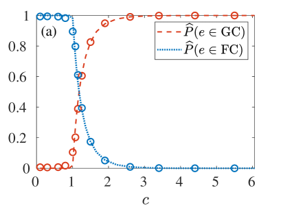
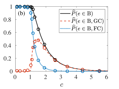
Figure 5: (Color online) (a) The probability $\widehat{P}(e\in{\rm GC})$ (dashed line), that a randomly sampled edge in an ER network resides on the giant component, as a function of the mean degree $c=\langle K\rangle$, obtained from Eq. (35); The complementary probability $\widehat{P}(e\in{\rm FC})$ (dotted line) that a randomly sampled edge resides on one of the finite components is also shown. (b) The probability $\widehat{P}(e\in{\rm B})$ (solid line) that a randomly sampled edge in an ER network is a bredge, as a function of the mean degree $c$, obtained from Eq. (73); The probability $\widehat{P}(e\in{\rm B})$ is equal to the sum of two components: the probability $\widehat{P}(e\in{\rm B},{\rm GC})$ (dashed line) that a randomly sampled edge is a bredge that resides on the giant component, and the probability $\widehat{P}(e\in{\rm B},{\rm FC})$ (dotted line) that a randomly sampled edge is a bredge that resides on one of the finite components. The analytical results are in excellent agreement with the results of computer simulations (circles), performed for an ensemble of ER networks of $N=10^{4}$ nodes.

In Fig. 5(a) we present analytical results for the probability $\widehat{P}(e\in{\rm GC})$ (dashed line), that a randomly sampled edge in an ER network resides on the giant component, as a function of the mean degree $c$. These results are obtained by inserting $\tilde{g}$ from Eq. (136) into Eq. (35). We also present the complementary probability $\widehat{P}(e\in{\rm FC})$ (dotted line) that a randomly sampled edge resides on one of the finite components. In Fig. 5(b) we present analytical reults for the probability $\widehat{P}(e\in{\rm B})$ (solid line) that a randomly sampled edge in an ER network is a bredge as a function of the mean degree $c$. The probability $\widehat{P}(e\in{\rm B})$ can be expressed as a sum of two components: the probability $\widehat{P}(e\in{\rm B},{\rm GC})=\widehat{P}(e\in{\rm B}|{\rm GC})\widehat{P}(e\in{\rm GC})$ (dashed line) that a randomly sampled edge is a bredge that resides on the giant component, and the probability $\widehat{P}(e\in{\rm B},{\rm FC})=\widehat{P}(e\in{\rm FC})$ (dotted line) that a randomly sampled edge is a bredge that resides on one of the finite components. The analytical results are in excellent agreement with the results of computer simulations (circles), performed for an ensemble of ER networks of $N=10^{4}$ nodes.

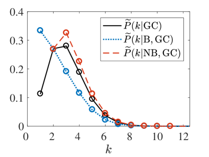
Figure 6: (Color online) Analytical results for the marginal degree distribution $\widetilde{P}(k|{\rm GC})$ (solid line) of end-nodes of randomly sampled edges, the marginal degree distribution $\widetilde{P}(k|{\rm B},{\rm GC})$ (dotted line) of end-nodes of randomly sampled bredges and the marginal degree distribution $\widetilde{P}(k|{\rm NB},{\rm GC})$ (dashed line) of randomly sampled non-bredge edges on the giant component of an ER network with mean degree $c=2$. The analytical results are in excellent agreement with the results obtained from computer simulations (circles).

In Fig. 6 we present analytical results for the marginal degree distribution $\widetilde{P}(k|{\rm GC})$ of end-nodes of edges on the giant component of an ER network (solid line), obtained by inserting $\tilde{g}$ from Eq. (136) into Eq. (41). We also present the marginal degree distribution $\widetilde{P}(k|{\rm B},{\rm GC})$ of end-nodes of bredges on the giant component (dotted line), obtained by inserting $\tilde{g}$ from Eq. (136) into Eq. (107) and for the marginal degree distribution $\widetilde{P}(k|{\rm NB},{\rm GC})$ of non-bredge edges that reside on the giant component (dashed line), obtained by inserting $\tilde{g}$ from Eq. (136) into Eq. (97). The analytical results are in excellent agreement with the corresponding results obtained from computer simulations (circles). It is found that the marginal degree distribution of the end-nodes of bredges decreases monotonically as a function of $k$, while the marginal degree distribution of the non-bredge edges exhibits a peak. Overall, the degrees of end-nodes of non-bredge edges tend to be higher than the degrees of end-nodes of bredges.

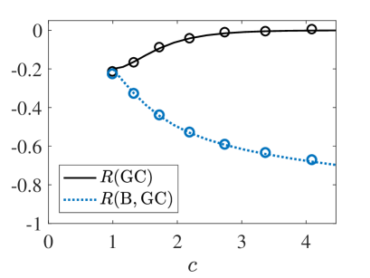
Figure 7: (Color online) Analytical results for the correlation coefficient $R({\rm GC})$ (solid line) between the degrees $k$ and $k^{\prime}$ of end-nodes of randomly sampled edges and the correlation coefficient $R({\rm B},{\rm GC})$ (dotted line) between the end-nodes of randomly sampled bredges that reside on the giant component of an ER network, as a function of the mean degree $c$. The analytical results are in excellent agreement with the results obtained from computer simulations (circles). The correlations, which are concentrated on the bredges, are negative and become stronger as $c$ is increased. Since the fraction of bredges on the giant component is a decreasing function of $c$, the correlation coefficient over all the edges on the giant component decreases (in absolute value) as $c$ is increased.

In Fig. 7 we present analytical results for the correlation coefficient $R({\rm GC})$ between the degrees of pairs of end-nodes of edges on the giant component of an ER network as a function of the mean degree $c$ (solid line), obtained by inserting $\tilde{g}$ from Eq. (136) into Eq. (72). We also present the correlation coefficient $R({\rm B},{\rm GC})$ between the degrees of end-nodes of bredges that reside on the giant component of an ER network (dotted line), obtained by inserting $\tilde{g}$ from Eq. (136) into Eq. (134). The analytical results are in excellent agreement with the results obtained from computer simulations (circles).

VII.2 Configuration model networks with exponential degree distributions

Consider a configuration model network with an exponential degree distribution of the form $P(k)\sim e^{-\alpha k}$, where $k_{\rm min}\leq k\leq k_{\rm max}$. In case that $k_{\rm min}\geq 2$ one can show that $g=\tilde{g}=1$ and there are no bredges. Here we consider the case of $k_{\rm min}=1$ and $k_{\rm max}=\infty$. In this case it is convenient to parametrize the degree distribution using the mean degree $c$ in the form

$$P(k)=\frac{1}{c-1}\left(\frac{c-1}{c}\right)^{k}.$$ (137)

In order to find the properties of bredges in such networks, we first calculate the parameters $\tilde{g}$ and $g$. Inserting the exponential degree distribution of Eq. (137) into the generating function $G_{1}(x)$, given by Eq. (3), we obtain $G_{1}(x)=[c-(c-1)x]^{-2}$. Inserting the above expression of $G_{1}(x)$ into Eq. (2) and solving for $\tilde{g}$, we find that for $c>3/2$ there is a non-trivial solution of the form

$$\tilde{g}=\frac{1}{2}\left[\frac{c-3}{c-1}+\sqrt{\frac{c+3}{c-1}}\right].$$ (138)

Inserting the exponential degree distribution of Eq. (137) into Eq. (6), we obtain $G_{0}(x)={x}/{[c-(c-1)x]}$. Inserting $\tilde{g}$ from Eq. (138) and the above expression of $G_{0}(1-\tilde{g})$ into Eq. (5), we find that for $c>3/2$

$$g=\frac{c}{2(c-1)}\left[3-\sqrt{\frac{c+3}{c-1}}\right].$$ (139)

Thus, it is found that the configuration model network with an exponential degree distribution exhibits a percolation transition at $c_{0}=3/2$.

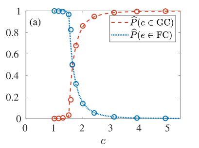
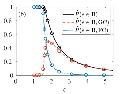
Figure 8: (Color online) (a) Analytical results for the probability $\widehat{P}(e\in{\rm GC})$ (dashed line) that a randomly sampled edge in a configuration model network with an exponential degree distribution resides on the giant component, as a function of the mean degree $c$; The complementary probability $P(e\in{\rm FC})$ (dotted line) that a randomly sampled edge resides on one of the finite tree components is also shown. (b) Analytical results for the probability $\widehat{P}(e\in{\rm B})$ (solid line) that a randomly sampled edge is a bredge, as a function of the mean degree $c$, obtained from Eq. (73); The probability $P(e\in{\rm B})$ is equal to the sum of two components: the probability $\widehat{P}(e\in{\rm B},{\rm GC})$ (dashed line), that a randomly sampled edge is a bredge that resides on the giant component and the probability $\widehat{P}(e\in{\rm B},{\rm FC})$ that a randomly sampled edge is a bredge that resides on one of the finite components. The analytical results are in excellent agreement with the results of computer simulations (circles), performed for an ensemble of configuration model networks of $N=10^{4}$ nodes.

In Fig. 8(a) we present the probability $\widehat{P}(e\in{\rm GC})$ (dashed line), that a random edge in a configuration model network with an exponential degree distribution resides on the giant component, obtained from Eq. (35), and the probability $\widehat{P}(e\in{\rm FC})$ (dotted line) that a random edge resides on one of the finite components, as a function of the mean degree $c$. In Fig. 8(b) we present the probability $\widehat{P}(e\in{\rm B})$ that a random edge in a configuration model network with an exponential degree distribution is a bredge (solid line), as a function of $c$, obtained from Eq. (73). We also present the probability $\widehat{P}(e\in{\rm B},{\rm GC})$ (dashed line) that a randomly selected edge in the network is a bredge that resides in the giant component and the probability $\widehat{P}(e\in{\rm B},{\rm FC})$ (dotted line) that a randomly selected edge in the network is a bredge that resides in one of the finite components. The analytical results are found to be in excellent agreement with the results of computer simulations (circles), performed for an ensemble of configuration model networks of $N=10^{4}$ nodes.

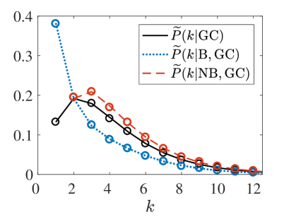
Figure 9: (Color online) Analytical results for the marginal degree distribution $\widetilde{P}(k|{\rm GC})$ (solid line) of end-nodes of randomly sampled edges, the marginal degree distribution $\widetilde{P}(k|{\rm B},{\rm GC})$ (dotted line) of end-nodes of randomly sampled bredges, and the marginal degree distribution $\widetilde{P}(k|{\rm NB},{\rm GC})$ (dashed line) of randomly sampled non-bredge edges, on the giant component of a configuration model network with an exponential degree distribution and mean degree $c=2.5$. The analytical results are in excellent agreement with the results obtained from computer simulations (circles).

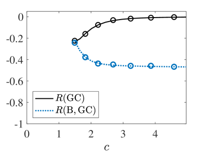
Figure 10: (Color online) Analytical results for the correlation coefficient $R({\rm GC})$ (solid line) between the degrees $k$ and $k^{\prime}$ of end-nodes of edges and the correlation coefficient $R({\rm B},{\rm GC})$ (dotted line) between the end-nodes of bredges that reside on the giant component of a configuration model network with an exponential degree distribution, as a function of the mean degree $c$. The analytical results are in excellent agreement with the results obtained from computer simulations (circles).

In Fig. 9 we present analytical results for the marginal degree distribution $\widetilde{P}(k|{\rm GC})$ of end-nodes of randomly selected edges (solid line), the marginal degree distribution $\widetilde{P}(k|{\rm B},{\rm GC})$ of end-nodes of bredges (dotted line) and the marginal degree distribution $\widetilde{P}(k|{\rm NB},{\rm GC})$ of non-bredge edges (dashed line) on the giant component of a configuration model network with an exponential degree distribution. The analytical results are in excellent agreement with the results obtained from computer simulations (circles).

In Fig. 10 we present analytical results for the correlation coefficients $R({\rm GC})$ and $R({\rm B},{\rm GC})$ between the degrees $k$ and $k^{\prime}$ of the end-nodes of edges that reside on the giant component (solid line) and bredges that reside on the giant component (dotted line), respectively, as a function of the mean degree $c$ in configuration model networks with exponential degree distributions. The analytical results are in excellent agreement with the results obtained from computer simulations (circles).

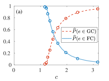
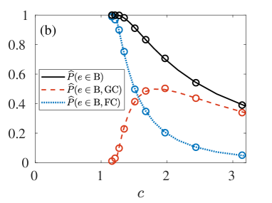
Figure 11: (Color online) (a) Analytical results for the probability $\widehat{P}(e\in{\rm GC})$ (dashed line) that a randomly sampled edge in a configuration model network with a power-law degree distribution resides on the giant component, as a function of the mean degree $c$. The complementary probability $\widehat{P}(e\in{\rm FC})$ (dotted line) that a randomly sampled edge resides on one of the finite tree components is also shown; (b) Analytical results for the probability $\widehat{P}(e\in{\rm B})$ (solid line) that a random edge is a bredge, as a function of the mean degree $c$. The probability $\widehat{P}(e\in{\rm B})$ is equal to the sum of two components: the probability $\widehat{P}(e\in{\rm B},{\rm GC})$ (dashed line) that a randomly sampled edge is a bredge that resides on the giant component and the probability $\widehat{P}(e\in{\rm B},{\rm FC})$ (dotted line) that a randomly sampled edge is a bredge that resides on one of the finite components. The analytical results are in excellent agreement with the results of computer simulations (circles), performed for networks of $N=10^{4}$ nodes.

VII.3 Configuration model networks with power-law degree distributions

Consider a configuration model network with a power-law degree distribution of the form $P(k)\sim k^{-\gamma}$, where $k_{\rm min}\leq k\leq k_{\rm max}$. For $\gamma\leq 2$ the mean degree diverges in the limit of $k_{\rm max}\rightarrow\infty$. For $2<\gamma\leq 3$ the mean degree is bounded while the second moment diverges. For $\gamma>3$ both moments are bounded. Here we focus on the case of $\gamma>2$, in which the mean degree, $\langle K\rangle$, is bounded even for $k_{\rm max}\rightarrow\infty$. We choose $k_{\rm min}=1$, for which there is a coexistence phase of the giant component and the finite tree components and $k_{\rm max}=100$. The normalized degree distribution is given by

$$P(k)=A(\gamma,k_{\rm max})\ k^{-\gamma},$$ (140)

where the normalization factor is $A(\gamma,k_{\rm max})=[\zeta(\gamma)-\zeta(\gamma,k_{\rm max}+1)]^{-1}$, the function $\zeta(\gamma,k)$ is the Hurwitz zeta function and $\zeta(\gamma)=\zeta(\gamma,1)$ is the Riemann zeta function Olver2010 . The mean degree is given by $\langle K\rangle=A(\gamma,k_{\rm max})/A(\gamma-1,k_{\rm max})$ and the second moment of the degree distribution is given by $\langle K^{2}\rangle=A(\gamma,k_{\rm max})/A(\gamma-2,k_{\rm max})$. Inserting the degree distribution of Eq. (140) into Eqs. (6) and (3) we obtain

$$G_{0}(x)=A(\gamma,k_{\rm max})\left[{\rm Li}_{\gamma}(x)-x^{k_{\rm max}+1}\Phi(x,\gamma,k_{\rm max}+1)\right],$$ (141)

and

$$xG_{1}(x) = A(\gamma-1,k_{\rm max})\Big{[}{\rm Li}_{\gamma-1}(x)$$ (142)

$$-x^{k_{\rm max}+1}\Phi(x,\gamma-1,k_{\rm max}+1)\Big{]},$$

where $\Phi(x,\gamma,k)$ is the Lerch transcendent and ${\rm Li}_{\gamma}(x)$ is the polylogarithm function Gradshteyn2000 . The values of the parameters $\tilde{g}$ and $g$ are determined by Eqs. (2) and (5). Unlike the ER network and the configuration model network with an exponential degree distribution, here we do not have closed form analytical expressions for $g$ and $\tilde{g}$. However, using the expressions above for $G_{0}(x)$ and $G_{1}(x)$, the values of $g$ and $\tilde{g}$ can be easily obtained from a numerical solution of Eqs. (2) and (5). Using the Molloy-Reed criterion Molloy1995 ; Molloy1998 , we find that for $k_{\rm max}=100$ the percolation threshold is $c_{0}\simeq 1.219$, where $\gamma_{0}\simeq 3.378$.

In Fig. 11(a) we present the probability $\widehat{P}(e\in{\rm GC})$ that a random edge in a configuration model network with a power-law degree distribution resides on the giant component (dashed line), obtained from Eq. (35), as a function of $c$. We also present the complementary probability $\widehat{P}(e\in{\rm FC})$ that a random edge resides on one of the finite components (dotted line). In Fig. 11(b) we present the probability $\widehat{P}(e\in{\rm B})$ that a random edge in a configuration model network with a power-law degree distribution is a bredge (solid line), as a function of $c$, obtained from Eq. (73). We also present the probability $\widehat{P}(e\in{\rm B},{\rm GC})$ (dashed line) that a randomly selected edge is a bredge that resides on the giant component and the probability $\widehat{P}(e\in{\rm B},{\rm FC})$ (dotted line) that a randomly selected edge is a bredge that resides on one of the finite tree components. The analytical results are in excellent agreement with the results of computer simulations (circles), performed for an ensemble of configuration model networks of $N=10^{4}$ nodes.

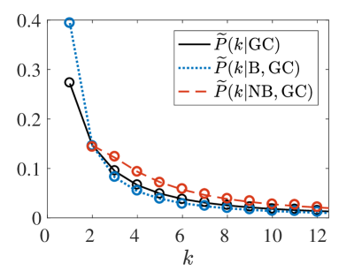
Figure 12: (Color online) Analytical results for the marginal degree distribution $\widetilde{P}(k|{\rm GC})$ of end-nodes of randomly selected edges (solid line), the marginal degree distribution $\widetilde{P}(k|{\rm B},{\rm GC})$ of end-nodes of bredges (dotted line) and the marginal degree distribution $\widetilde{P}(k|{\rm NB},{\rm GC})$ of end-nodes of non-bredge edges (dashed line) on the giant component of a configuration model network with a power-law degree distribution with an exponent $\gamma=2.5$ and mean degree $c=1.54$. The analytical results are in excellent agreement with the results obtained from computer simulations (circles).

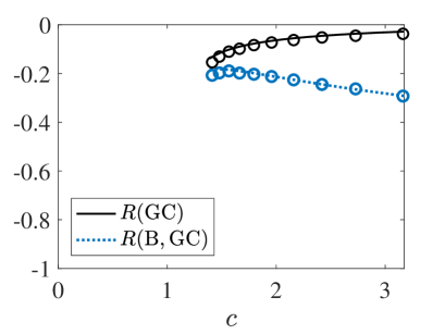
Figure 13: (Color online) Analytical results for the correlation coefficient $R({\rm GC})$, between the degrees $k$ and $k^{\prime}$ of end-nodes of edges (solid line) and the correlation coefficient $R({\rm B},{\rm GC})$ between the end-nodes of bredges (dotted line) that reside on the giant component of a configuration model network with a power-law degree distribution, as a function of the mean degree $c$. The analytical results are in excellent agreement with the results obtained from computer simulations (circles), except for the dilute network regime just above the percolation transition. In this regime the giant component is small and its size fluctuates between different network instances. The data points in this regime were averaged over 100 network instances, while all the other data points were averaged over 20 network instances.

In Fig. 12 we present analytical results for the marginal degree distribution $\widetilde{P}(k|{\rm GC})$ of end-nodes of randomly selected edges (solid line), the marginal degree distribution $\widetilde{P}(k|{\rm B},{\rm GC})$ of end-nodes of bredges (dotted line) and the marginal degree distribution $\widetilde{P}(k|{\rm NB},{\rm GC})$ of non-bredge edges (dashed line) on the giant component of a configuration model network with a power-law degree distribution. The analytical results are in excellent agreement with the results obtained from computer simulations (circles).

In Fig. 13 we present analytical results for the correlation coefficient $R({\rm GC})$, between the degrees $k$ and $k^{\prime}$ of end-nodes of edges (solid line) and the correlation coefficient $R({\rm B},{\rm GC})$ between the end-nodes of bredges (dotted line) that reside on the giant component of a configuration model network with a power-law degree distribution, as a function of the mean degree $c$. The analytical results are in excellent agreement with the results obtained from computer simulations (circles) except for the dilute network regime where there are noticeable deviations due to finite size effects.

In the case of infinite networks, one may consider the limit of $k_{\rm max}\rightarrow\infty$. In this limit the expression for the degree distribution is simplified to $P(k)=k^{-\gamma}/\zeta(\gamma)$. For $\gamma>2$ the mean degree is given by $\langle K\rangle=\zeta(\gamma-1)/\zeta(\gamma)$ and for $\gamma>3$ the second moment is given by $\langle K^{2}\rangle=\zeta(\gamma-2)/\zeta(\gamma)$. The generating functions are simplified to $G_{0}(x)={\rm Li}_{\gamma}(x)/\zeta(\gamma)$ and $xG_{1}(x)={\rm Li}_{\gamma-1}(x)/\zeta(\gamma-1)$. Using the Molloy-Reed criterion Molloy1995 ; Molloy1998 , we find that for $k_{\rm max}\rightarrow\infty$ the percolation threshold is $c_{0}\simeq 1.196$, where $\gamma_{0}\simeq 3.478$.

VIII Discussion

Transportation, communication and many other networks consist of a single connected component, in which there is at least one path connecting any pair of nodes. This property is essential for the functionality of these networks. The failure of a node or an edge disconnects the paths that go through the failed node/edge. In case that the failed node is an AP or the failed edge is a bredge, the disconnected paths have no substitute. As a result, a whole patch of nodes becomes disconnected from the rest of the network. Networks that do not include any APs and bredges are called biconnected networks Newman2008 ; Dufresne2013 . In such networks, any node $i$ is connected to any other node $j$ by at least two non-overlapping paths. While biconnected networks are resilient to the deletion of a single node or a single edge, they are still vulnerable to multiple node/edge deletions. This is due to the fact that the deletion of a node/edge may turn other nodes into APs and other edges into bredges. Their subsequent deletion would disconnect other nodes from the rest of the network. The properties of APs and bredges are utilized in optimized algorithms of network dismantling Braunstein2016 ; Zdeborova2016 ; Wandelt2018 ; Ren2019 . The first stage of these dismantling processes is the decycling stage in which one node is deleted in each cycle, transforming the network into a tree network. In tree networks all the nodes of degrees $k\geq 2$ are APs and all the edges are bredges. Thus the deletion of such nodes/edges efficiently breaks the network into many small components.

The properties of bredges in a wide range of real-world empirical networks were recently studied Wu2018 . The fraction of bredges in each network was calculated using an algorithm based on depth-first search. An ensemble of configuration model networks, whose degree distribution coincides with the degree sequence of the empirical network, was generated using degree-preserving randomization. The fraction of bredges in each ensemble was calculated both numerically and using a generating function formalism. It was found that the fraction of bredges in the randomized ensembles is very similar to their fraction in the corresponding empirical networks. This indicates that the information about the number of bredges is captured in the degree distribution. Therefore, correlations and other structural properties that distinguish an empirical network from the corresponding configuration model network were found to have little effect on the number of bredges.

The edges in a network can be considered as the building blocks of paths connecting pairs of nodes. Pairs of nodes that reside on the same network component may be connected to each other by multiple paths. Among the paths connecting a pair of nodes $i$ and $j$, the shortest paths are of particular importance because they are likely to provide the fastest and strongest interactions. The statistical properties of the shortest paths are captured by the distribution of shortest path lengths (DSPL). The DSPL can be used to characterize the large scale structure of the network, in analogy to the degree destribution which is used to characterize the local structure. Central measures of the DSPL such as the mean distance Bollobas2001 ; Chung2003 ; Fronczak2004 ; Durrett2007 and extremal measures such as the diameter Hartmann2017 were studied. However, apart from a few studies Newman2001 ; Dorogovtsev2003 ; Blondel2007 ; Hofstad2008 ; Esker2008 ; Shao2008 ; Shao2009 the DSPL has not attracted nearly as much attention as the degree distribution. Recently, an analytical approach was developed for calculating the DSPL in the (ER) network Katzav2015 , followed by more general formulations that apply to configuration model networks Nitzan2016 ; Melnik2016 ; Katzav2018 , to modular networks Asher2020 and to networks that form by kinetic growth processes Steinbock2017 ; Steinbock2019a ; Steinbock2019b .

The importance of a given edge $e$ in a network may be quantified by its betweeness centrality, which is the number of pairs of nodes $i$ and $j$, such that of shortest paths between them pass through $e$ Freeman1977 ; Goh2003 . In general, the calculation of the betweeness centrality of an edge cannot be done locally. It involves the calculation of the shortest paths between all the pairs of nodes in the network, which requires access to the structure of the whole network Brandes2001 . However, in case that an edge $e$ is a bredge, one can easily obtain its betweeness centrality. Consider a bredge $e$ that resides on the giant component whose size is $N_{\rm GC}$. If the deletion of $e$ detaches a tree component of size $N_{\rm FC}$ from the giant component, the betweeness centrality of $e$ is given by $\beta_{e}=N_{\rm FC}(N_{\rm GC}-N_{\rm FC})$.

The damage exerted on a network upon deletion of a bredge can be evaluated using a centrality measure called bridgeness Wu2018 . The bridgeness of a bredge $e$ that resides on the giant component is defined as the number of nodes disconnected from the giant component upon deletion of $e$. The bridgeness of bredges that reside on the finite components is zero. Using a generating function formulation derived earlier to calculate the size distribution of the finite tree components Newman2007 ; Kryven2017 , Wu et al. obtained the bridgeness distribution in configuration model networks with Poisson, exponential and power-law degree distributions Wu2018 . It was found that the mean bridgeness diverges at $c\rightarrow c_{0}^{+}$ and and monotonically decreases as the mean degree is increased.

Another useful measure of the importance of an edge $e$ in a network is given by its range $\rho$, which is the distance between its end-nodes $i$ and $i^{\prime}$ in the reduced network from which $e$ is removed Granovetter1973 ; Granovetter1983 . In the special case in which $e$ is a bredge, its range is $\rho=\infty$, because upon deletion of $e$ its end-nodes land on different network components. For edges that are not bredges the range $\rho\geq 2$ is finite. It is equal to the shortest path length between $i$ and $i^{\prime}$ in the reduced network. It also satisfies $\rho=\ell-1$ where $\ell$ is the length of the shortest cycle that includes the edge $e$ in the original network. Edges whose range $\rho$ is large are considered important because upon their removal the shortest alternate path between $i$ and $i^{\prime}$ is large. In practical applications, large $\rho$ implies long and potentially costly delays in communication and transportation in case that the edge $e$ fails.

Figure 14: (Color online) ER networks of $N=100$ nodes with mean degree $c=1.1$ (a) and $c=1.7$ (b), which exhibit a coexistence between a giant component and finite tree components. The non-bredge edges (solid lines) connect pairs of nodes that reside on the 2-core of the giant component. In the more dilute case (a) the 2-core consists of a single cycle, while in the denser case (b) it exhibits a complex web of cycles. The root bredges (dashed lines) connect the tree branches on the giant component to the 2-core. All the other bredges (dotted lines) connect pairs of nodes on that reside on the tree branches of the giant component and pairs of nodes on the finite tree components.

In Fig. 14 we present ER networks of $N=100$ nodes with mean degrees $c=1.1$ [Fig. 14(a)] and $c=1.7$ [Fig. 14(b)]. In both networks the giant component coexists with many finite components. The non-bredge edges (solid lines) connect pairs of nodes that reside on the 2-core of the giant component Newman2008 ; Dufresne2013 . The giant component is decorated by tree branches, on which all the edges are bredges. The bredge that connects each tree branch to the 2-core of the giant component is called root bredge (dashed line). The end-node of the root bredge that resides on the 2-core is called root end-node. All the other bredges (dotted lines) connect pairs of nodes that reside on the tree branches, which are not on the 2-core. The average size of the tree branches that decorate the giant component is given by Wu2018

$$N_{\rm T}=\frac{1}{1-G^{\prime}_{1}(1-\tilde{g})},$$ (143)

which is the sum of a geometric series whose ratio $G^{\prime}_{1}(1-\tilde{g})$ is the excess degree of the end-nodes of the finite component side of the bredges, whose degree distribution is given by Eq. (102). Thus, the fraction of root end-nodes among the end-nodes on the GC side of bredges on the giant component is $1/N_{\rm T}$. The degree distribution of the root end-nodes, which reside on the 2-core of the giant component, is given by

$$\widetilde{P}(K_{\scriptsize{\mbox{2-CORE}}}=k|{\rm B},{\rm GC})$$ (144)

$$=\frac{\left[1-(1-\tilde{g})^{k-1}\right]-(k-1)\tilde{g}(1-\tilde{g})^{k-2}}{\tilde{g}[1-G^{\prime}_{1}(1-\tilde{g})]}\widetilde{P}(k).$$

The degree distribution of the end-nodes on the GC sides of all other bredges, which reside on the 1-core of the giant component is given by

$$\widetilde{P}(K_{{\rm GC}\cap\overline{\scriptsize{\mbox{2-CORE}}}}=k|{\rm B},{\rm GC})=\frac{(k-1)(1-\tilde{g})^{k-2}}{G^{\prime}_{1}(1-\tilde{g})}\widetilde{P}(k).$$ (145)

The overall distribution of the degrees $K_{\rm GC}$, given by Eq. (101), is recovered by

$$\widetilde{P}(K_{\rm GC} = k|{\rm B},{\rm GC})=\frac{1}{N_{\rm T}}\widetilde{P}(K_{\scriptsize{\mbox{2-CORE}}}=k|{\rm B},{\rm GC})$$ (146)

$$+\left(1-\frac{1}{N_{\rm T}}\right)\widetilde{P}(K_{{\rm GC}\cap\overline{\scriptsize{\mbox{2-CORE}}}}=k|{\rm B},{\rm GC}).$$

The distinction between root bredges and all the other bredges on the giant component may be useful for optimized dismantling algorithms and targeted attacks. This is due to the fact that the deletion of a root bredge disconnects the whole tree branch that is held by this bredge. In contrast, random deletion of bredges may require a large number of deletion steps in order to chop each tree branch from the 2-core of the giant component.

IX Summary

We presented analytical results for the statistical properties of edges and bredges in configuration model networks. To quantify the abundance of bredges, we calculated the probability $\widehat{P}(e\in{\rm B})$ that a random edge $e$ in a configuration model network with a given degree distribution $P(k)$ is a bredge. We also obtained the conditional probability $\widehat{P}(e\in{\rm B}|k,k^{\prime})$ that a random edge whose end-nodes are of degrees $k$ and $k^{\prime}$ is a bredge. Using Bayes’ theorem, we obtained the joint degree distribution $\widehat{P}(k,k^{\prime}|{\rm B})$ of the end-nodes of randomly sampled bredges. We also studied the distinct properties of bredges on the giant component and on the finite components. On the finite components all the edges are bredges, namely $\widehat{P}(e\in{\rm B}|{\rm GC})=1$, and there are no degree-degree correlations. We calculated the probability $\widehat{P}(e\in{\rm B}|{\rm GC})$ that a random edge on the giant component is a bredge. We also obtained the joint degree distribution $\widehat{P}(k,k^{\prime}|{\rm B},{\rm GC})$ of the end-nodes of bredges and the joint degree distribution $\widehat{P}(k,k^{\prime}|{\rm NB},{\rm GC})$ of the end-nodes of non-bredge (NB) edges on the giant component. Surprisingly, it was found that the degrees $k$ and $k^{\prime}$ of the end-nodes of bredges are correlated, while the degrees of the end-nodes of non-bredge edges are uncorrelated. This implies that all the degree-degree correlations on the giant component are concentrated on the bredges. We calculated the covariance $\Gamma({\rm B},{\rm GC})$ and found that it is negative, which means that bredges on the giant component tend to connect high degree nodes to low degree nodes and vice versa. We applied this analysis to ensembles of configuration model networks with degree distributions that follow a Poisson distribution (Erdős-Rényi networks), an exponential distribution and a power-law distribution (scale-free networks). The implications of these results were discussed in the context of common attack scenarios and network dismantling processes.

This work was supported by the Israel Science Foundation grant no. 1682/18.

References

- (1) S. Havlin and R. Cohen, Complex Networks: Structure, Robustness and Function (Cambridge University Press, New York, 2010).
- (2) M.E.J. Newman, Networks: an Introduction, 1st Edition (Oxford University Press, Oxford, 2010).
- (3) E. Estrada, The Structure of Complex Networks: Theory and Applications (Oxford University Press, Oxford, 2011).
- (4) A. Barrat, M. Barthélemy and A. Vespignani, Dynamical Processes on Complex Networks (Cambridge University Press, Cambridge, 2012).
- (5) V. Latora, V. Nicosia, G. Russo, Complex Networks: Principles, Methods and Applications, (Cambridge University Press, Cambridge, 2017).
- (6) B. Bollobás, Random Graphs, 2nd Edition (Cambridge University Press, Cambridge, 2001).
- (7) R. Albert, H. Jeong and A.-L. Barabási, Error and attack tolerance of complex networks, Nature 406, 378 (2000).
- (8) R. Cohen, K. Erez, D. ben-Avraham and S. Havlin, Resilience of the internet to random breakdowns, Phys. Rev. Lett. 85, 4626 (2000).
- (9) R. Cohen, K. Erez, D. ben-Avraham and S. Havlin, Breakdown of the internet under intentional attack, Phys. Rev. Lett. 86, 3682 (2001).
- (10) C.M. Schneider, A.A. Moreira, J.S. Andrade, S. Havlin and H.J. Herrmann, Mitigation of malicious attacks on networks, Proc. Natl. Acad. Sci. USA 108, 3838 (2011).
- (11) J. Hopcroft and R. Tarjan, Efficient algorithms for graph manipulation, Communications of the ACM 16, 372 (1973).
- (12) A. Gibbons, Algorithmic Graph Theory (Cambridge University Press, Cambridge, 1985).
- (13) P. Chaudhuri, An optimal distributed algorithm for finding afticulation points in a network, Computer Communications 21, 1707 (1998).
- (14) L. Tian, A. Bashan, D.-N. Shi and Y.-Y. Liu, Articulation points in complex networks, Nature Communications 8, 14223 (2017).
- (15) G.F. Italiano, L. Laura and F. Santaroni, Finding strong bridges and strong articulation points in linear time, Theoretical Computer Science 447, 74 (2012).
- (16) R.E. Tarjan, A note on finding the bridges of a graph, Information Processing Letters 2, 160 (1974).
- (17) B. Bollobas, Modern Graph Theory (Springer, New York, 1998).
- (18) The word ’bredge’ is an obsolete form of the word ’bridge’ in ancient English; See e.g. English Dictionary, explaining the difficult terms, by E. Coles, School-Master and Teacher, printed for Peter Parker at the Leg and Star over against the Royal-Exchange in Cornbil (1685).
- (19) A. Braunstein, L. Dall’Asta, G. Semerjian and L. Zdeborová, Network dismantling, Proc. Natl. Acad. Sci. USA 113, 12368 (2016).
- (20) L. Zdeborová, P. Zhang and H.-J. Zhou, Fast and simple decycling and dismantling of networks, Scientific Reports 6, 37954 (2016).
- (21) S. Wandelt, X. Sun, D. Feng, M. Zanin and S. Havlin, A comparative analysis of approaches to network-dismantling, Scientific Reports 8, 13513 (2018).
- (22) X.-L. Ren, N. Gleinig, D. Helbing and N. Antulov-Fantulina, Generalized network dismantling, Proc. Natl. Acad. Sci. USA 116, 6554 (2019).
- (23) I. Tishby, O. Biham, R. Kühn and E. Katzav, Statistical analysis of articulation points in configuration model networks, Phys. Rev. E 98, 062301 (2018).
- (24) M. Molloy and B. Reed, A critical point for random graphs with a given degree sequence, Random Struct. Algorithms 6, 161 (1995).
- (25) M. Molloy and B. Reed, The size of the giant component of a random graph with a given degree sequence, Combinatorics, Probability and Computing 7, 295 (1998).
- (26) M.E.J. Newman, S.H. Strogatz and D.J. Watts, Random graphs with arbitrary degree distributions and their applications, Phys. Rev. E 64, 026118 (2001).
- (27) P. Erdős and T. Gallai, Gráfok előírt fokszámú pontokkal, Matematikai Lapok 11, 264 (1960).
- (28) S.A. Choudum, A simple proof of the Erdős-Gallai theorem on graph sequences, Bulletin of the Australian Mathematical Society 33, 67 (1986).
- (29) H. Bonneau, A. Hassid, O. Biham, R. Kühn and E. Katzav, Distribution of shortest cycle lengths in random networks, Phys. Rev. E 96, 062307 (2017).
- (30) M. Mézard, G. Parisi and M.A. Virasoro, Random free energies in spin glasses, J. Physique Lett. 46, L217 (1985).
- (31) M. Mézard and G. Parisi, The cavity method at zero temperature, J. Stat. Phys. 111, 1 (2003).
- (32) M. Mézard and A. Montanari, Information, Physics and Computation (Oxford University Press, Oxford, 2009).
- (33) G. Del Ferraro, C. Wang, D. Martí and M. Mézard, Cavity method - message passing from a physics perspective, Statistical Physics, Optimization, Inference and Message-Passing Algorithms, Lecture Notes of the Les Houches School of Physics, Eds. F. Krzakala, F. Ricci-Tersenghi, L. Zdeborova, R. Zecchina, E.W. Tramel, and L.F. Cugliandolo (Oxford University Press, Oxford, 2015).
- (34) A. Lowy and P. Wood, The power of the matrix: using thinking to solve business problems and make better decisions (Jossey Bass, San Francisco, 2004)
- (35) I. Tishby, O. Biham, E. Katzav and R. Kühn, Revealing the microstructure of the giant component in random graph ensembles, Phys. Rev. E 97, 042318 (2018).
- (36) I. Tishby, O. Biham, E. Katzav and R. Kühn, Generating random networks that consist of a single connected component with a given degree distribution, Phys. Rev. E 99, 042308 (2019).
- (37) S.B. Seidman, Network structure and minimum degree, Social Networks 5, 269 (1983).
- (38) X. Yuan, Y. Dai, H.E. Stanley and S. Havlin, k-core percolation on complex networks: Comparing random, localized, and targeted attacks, Phys. Rev. E 93, 062302 (2016).
- (39) S.N. Dorogovtsev, A.V. Goltsev and J.F.F. Mendes, k-Core Organization of Complex Networks, Phys. Rev. Lett. 96, 040601 (2006).
- (40) S.N. Dorogovtsev, A.V. Goltsev and J.F.F. Mendes, k-core architecture and k-core percolation on complex networks, Physica D 224, 7 (2006).
- (41) O. Diekmann and J.A.P. Heesterbekk, Mathematical Epidemiology of Infectious Diseases: Model Building, Analysis and Interpretation (John Wiley & Sons, Chichester, 2000).
- (42) J. Duderstadt and L. Hamilton, Nuclear Reactor Analysis (John Wiley & Sons, USA, 1976)
- (43) E. Katzav, O. Biham and A. Hartmann, Metric properties of subcritical Erdős-Rényi networks, Phys. Rev. E 98, 012301 (2018).
- (44) M.E.J. Newman, Assortative mixing in networks, Phys. Rev. Lett. 89, 208701 (2002).
- (45) M.E.J. Newman, Mixing patterns in networks, Phys. Rev. E 67, 026126 (2003).
- (46) M.E.J. Newman and J. Park, Why social networks are different from other types of networks, Phys. Rev. E 68, 036122 (2003).
- (47) S. Johnson, J.J. Torres, J. Marro and M.A. Munoz, Entropic Origin of Disassortativity in Complex Networks, Phys. Rev. Lett. 104, 108702 (2010).
- (48) S. Mizutaka and T. Hasegawa, Disassortativity of percolating clusters in random networks, Phys. Rev. E 98, 062314 (2018).
- (49) A.-K. Wu, L. Tian and Y.-Y. Liu, Bridges in complex networks, Phys. Rev. E 97, 012307 (2018).
- (50) P. Erdős and Rényi, On random graphs I, Publicationes Mathematicae 6, 290 (1959).
- (51) P. Erdős and Rényi, On the evolution of random graphs Publ. Math. Inst. Hung. Acad. Sci. 5, 17 (1960).
- (52) P. Erdős and Rényi, On the evolution of random graphs II Bull. Inst. Int. Stat. 38, 343 (1961).
- (53) F.W.J. Olver, D.M. Lozier, R.F. Boisvert and C.W. Clark, NIST Handbook of Mathematical Functions (Cambridge University Press, Cambridge, 2010).
- (54) I.S. Gradshteyn and I.M. Ryzhik, Tables of Integrals, Series, and Products, 6th edition (Academic Press, San Diego, 2000).
- (55) M.E.J. Newman and G. Ghoshal, Bicomponents and the robustness of networks to failure, Phys. Rev. Lett. 100, 138701 (2008).
- (56) L. Hébert-Dufresne, A. Allard, J.-G. Young, and L.J. Dubé, Percolation on random networks with arbitrary k-core structure, Phys. Rev. E 88, 062820 (2013).
- (57) F. Chung and L. Lu, The average distance in a random graph with given expected degrees, Internet Mathematics 1, 91 (2003).
- (58) A. Fronczak, P. Fronczak, and J.A. Holyst, Average path length in random networks, Phys. Rev. E 70, 056110 (2004).
- (59) R. Durrett, Random Graph Dynamics (Cambridge University Press, Cambridge, 2007)
- (60) A.K. Hartmann, M. Mézard, Phys. Rev. E 97, 032128 (2017)
- (61) S.N. Dorogovtsev, J.F.F. Mendes and A.N. Samukhin, Metric structure of random networks, Nuclear Physics B 653, 307 (2003).
- (62) V.D. Blondel, J.-L. Guillaume, J.M. Hendrickx and R.M. Jungers, Distance distribution in random graphs and application to network exploration, Phys. Rev. E 76, 066101 (2007).
- (63) R. van der Hofstad and G. Hooghiemstra, Universality for distances in power-law random graphs, J. Math. Phys. 49, 125209 (2008).
- (64) H. van der Esker, R. van der Hofstad, G. Hooghiemstra, Universality for the Distance in Finite Variance Random Graphs, J. Stat. Phys. 133, 169 (2008).
- (65) J. Shao, S.V. Buldyrev, R. Cohen, M. Kitsak, S. Havlin and H.E. Stanley, EPL 84, 48004 (2008).
- (66) J. Shao, S.V. Buldyrev, L.A. Braunstein, S. Havlin and H.E. Stanley, Structure of shells in complex networks Phys. Rev. E 80, 036105 (2009).
- (67) E. Katzav, M. Nitzan, D. ben-Avraham, P.L. Krapivsky, R. Kühn, N. Ross and O. Biham, Analytical results for the distribution of shortest path lengths in random networks, EPL 111, 26006 (2015).
- (68) M. Nitzan, E. Katzav, R. Kühn and O. Biham, Distance distribution in configuration-model networks, Phys. Rev. E 93, 062309 (2016).
- (69) S. Melnik and J.P. Gleeson, Simple and accurate analytical calculation of shortest path lengths, arXiv:1604.05521.
- (70) E.E. Asher, H. Sanhedrai, N.K. Panduranga, R. Cohen and S. Havlin, Distance distribution in extreme modular networks, Phys. Rev. E 101, 022313 (2020)
- (71) C. Steinbock, O. Biham and E. Katzav, The distribution of shortest path lengths in a class of node duplication network models, Phys. Rev. E 96, 032301 (2017).
- (72) C. Steinbock, O. Biham and E. Katzav, Analytical results for the distribution of shortest path lengths in directed random networks that grow by node duplication, Europ. Phys. J. B 92, 130 (2019).
- (73) C. Steinbock, O. Biham and E. Katzav, Analytical results for the in-degree and out-degree distributions of directed random networks that grow by node duplication, J. Stat. Mech. 083403 (2019).
- (74) L.C. Freeman, A set of measures of centrality based on betweenness, Sociometry 40, 35 (1977).
- (75) K.I. Goh, E. Oh, B. Kahng and D. Kim, Betweenness centrality correlation in social networks Phys. Rev. E 67, 017101 (2003).
- (76) U. Brandes, A faster algorithm for betweenness centrality, Journal of Mathematical Sociology 25, 163 (2001).
- (77) M.E.J. Newman, Component sizes in networks with arbitrary degree distributions Phys. Rev. E 76, 045101 (2007).
- (78) I. Kryven, General expression for the component size distribution in infinite configuration networks, Phys. Rev. E 95, 052303 (2017).
- (79) M. Granovetter, The strength of weak ties, American Journal of Sociology 78, 1360 (1973).
- (80) M. Granovetter, The strength of weak ties: a network theory revisited, Sociological Theory 1, 201 (1983).