On the molecular information revealed by photoelectron angular distributions of isotropic samples

Abstract

We propose an alternative approach to the description and analysis of photoelectron angular distributions (PADs) resulting from isotropic samples in the case of few-photon absorption via electric fields of arbitrary polarization. As we demonstrate for the one- and two-photon cases, this approach reveals the molecular frame information encoded in the $b_{l,m}$ expansion coefficients of the PAD in a particularly clear way. Our approach does not rely on explicit partial wave expansions of the scattering wave function and the expressions we obtain are therefore interpreted in terms of the vector field structure of the photoionization dipole $\vec{D}(\vec{k})$ as a function of the photoelectron momentum $\vec{k}$. This provides very compact expressions that reveal how molecular rotational invariants couple to the setup (electric field polarization and detectors) rotational invariants. We rely heavily on this approach in a companion paper on tensorial chiral setups. Here we apply this approach to one-photon ionization and find that while $b_{0,0}$ depends only on the magnitude of $\vec{D}(\vec{k})$, $b_{1,0}$ (non-zero for chiral molecules) is sensitive only to the components of $\vec{D}(\vec{k})$ perpendicular to $\vec{k}$ encoded in the propensity field $\vec{B}(\vec{k})\equiv i\vec{D}^{*}(\vec{k})\times\vec{D}(\vec{k})$, and $b_{2,0}$ is sensitive only to the the component of $\vec{D}(\vec{k})$ along $\vec{k}$. We also analyze the resonantly enhanced two-photon case where we show that $b_{0,0}$ and $b_{1,0}$ can be written in terms of an effectively stretched $\vec{D}(\vec{k})$, and that $b_{1,0}$ and $b_{3,0}$ reveal structural information of the field $\vec{B}(\vec{k})$ encoded in three of its vector spherical harmonic expansion coefficients.

I Introduction

Photoelectrons provide an important window into the structure of matter. In the case of gas phase molecules it is remarkable that part of that structural information, which goes beyond the energy spectrum of the molecule, is imprinted in the PAD even when the molecules are randomly oriented in space. A paramount example of this is photoelectron circular dichroism (PECD), where the opposite enantiomers of a chiral molecule (sharing the same energy spectrum) yield markedly different PADs when illuminated with circularly polarized light Ritchie (1976); Powis (2008). Motivated by the importance of enantiomeric recognition for the chemical industry and by the fact that it occurs already within the electric-dipole approximation and yields very strong enantiosensitive signals, PECD has been studied across a wide range of molecular species Ulrich et al. (2008); Nahon et al. (2015) and photoionization regimes Lux et al. (2012); Garcia et al. (2013); Dreissigacker and Lein (2014); Beaulieu et al. (2016, 2017); Turchini (2017). Crucially, the extension of PECD into the realm of multiphoton ionization provides both access to time-resolved ultra-fast enantiosensitive electronic dynamics Beaulieu et al. (2017); Comby et al. (2016); Beaulieu et al. (2018); Ordonez and Smirnova (2018) and the means to control the enantiosensitive signal observed in the PAD Demekhin et al. (2018); Goetz et al. (2019).

The interpretation of these and other exciting yet intricate phenomena relies on the mathematical formulation available for the description of PADs in molecules. A cornerstone of this formulation is the partial wave expansion of the scattering wave function, which is normally performed at the outset of any PAD derivation Ritchie (1976); Powis (2008); Tully et al. (1968); Chandra (1987); Reid (2003), in preparation for the orientation averaging step. Here we show that one can arrive to insightful orientation-averaged expressions for the $b_{l,m}$ coefficients describing the PAD without invoking the expansion of the scattering wave function. In fact, doing so reveals interesting physics that would be otherwise obscured by the partial wave expansion itself. We already took advantage of a restricted version of this approach (valid only for the $b_{1,0}$ coefficient) in the analysis of one- and two-photon ionization of chiral samples Beaulieu et al. (2018); Ordonez and Smirnova (2018, 2019a). There it played a fundamental role in the interpretation of the phenomena and in establishing connections to other enantiosensitive effects occurring within the electric-dipole approximation Giordmaine (1965); Patterson et al. (2013); Patterson and Doyle (2013) as well as to a geometrical effect in solids Yao et al. (2008).

With this approach at our disposal we ask a simple question. What is the meaning of the molecular information encoded in the orientation-averaged $b_{l,m}$ coefficients? Can it be understood as something else besides the complex interference of (potentially many $\sim 15$ Powis (2008); Stener et al. (2004); Giardini et al. (2005); Harding and Powis (2006); Tommaso et al. (2006)) partial waves with different phase shifts? Since the photoionization is determined by the photoionization dipole $\vec{D}(\vec{k})\equiv\langle\vec{k}|\hat{\vec{d}}|0\rangle$ between the ground state and the scattering state, each of the $b_{l,m}$ coefficients should tell us something different about the structure of $\vec{D}(\vec{k})$. Furthermore, since we are dealing with isotropic samples only rotational invariants of the molecule and of the setup (electric field polarization and detectors) can be part of the answer. How are these coupled to each other? Here we provide a method to approach these questions in general, and provide concrete and perhaps surprisingly simple answers for the case of all $b_{l,m}$ coefficients in one-photon ionization with arbitrary polarization and for the coefficients $b_{0,0},$ $b_{1,0}$, and $b_{3,0}$ in two-photon ionization with circularly polarized light. We will also make extensive use of this approach in a companion paper Ordonez and Smirnova dealing with tensorial chiral setups and a novel type of enantiosensitive asymmetries in PADs Demekhin et al. (2018); Demekhin (2019).

The paper is organized as follows: in Sec. II we present the main derivation for the $b_{l,m}$ coefficients in multiphoton ionization with fields of arbitrary polarization. Section III contains the analysis of one-photon ionization and Sec. IV the analysis of two-photon resonantly-enhanced ionization. Section V summarizes the conclusions of this work.

II General methodology

The photoionization of an isotropic molecular sample results in a photoelectron spectrum $W^{\mathrm{L}}(\vec{k}^{\mathrm{L}})$ given by

$$W^{\mathrm{L}}(\vec{k}^{\mathrm{L}})=\int\mathrm{d}\varrho\,W^{\mathrm{L}}(\vec{k}^{\mathrm{L}},\varrho)$$ (1)

where $W^{\mathrm{L}}(\vec{k}^{\mathrm{L}},\varrho)$ is the photoelectron spectrum for a given molecular orientation $\varrho\equiv\alpha\beta\gamma$, $\alpha\beta\gamma$ are the Euler angles, $\int\mathrm{d}\varrho\equiv\frac{1}{8\pi^{2}}\int_{0}^{2\pi}\mathrm{d}\alpha\int_{0}^{\pi}\mathrm{d}\beta\int_{0}^{2\pi}\mathrm{d}\gamma$ is the integral over all orientations, and the superscript $\mathrm{L}$ indicates vectors and functions in the laboratory frame. Since we can always expand $W^{\mathrm{L}}(\vec{k}^{\mathrm{L}})$ into real spherical harmonics $\tilde{Y}_{l}^{m}(\hat{k}^{\mathrm{L}})$,

$$W^{\mathrm{L}}(\vec{k}^{\mathrm{L}}) =\sum_{l,m}\tilde{b}_{l,m}\left(k\right)\tilde{Y}_{l}^{m}(\hat{k}^{\mathrm{L}}),$$ (2)

then any information about the molecule and the ionizing field encoded in the photoelectron spectrum $W^{\mathrm{L}}(\vec{k}^{\mathrm{L}})$ is now neatly summarized in the expansion coefficients $\tilde{b}_{l,m}\left(k\right)$,

$$\tilde{b}_{l,m}\left(k\right) =\int\mathrm{d}\Omega_{k}^{\mathrm{L}}\tilde{Y}_{l}^{m}(\hat{k}^{\mathrm{L}})W^{\mathrm{L}}(\vec{k}^{\mathrm{L}}),$$

$$=\int\mathrm{d}\Omega_{k}^{\mathrm{L}}\tilde{Y}_{l}^{m}(\hat{k}^{\mathrm{L}})\int\mathrm{d}\varrho\,W^{\mathrm{L}}(\vec{k}^{\mathrm{L}},\varrho),$$ (3)

where $\int\mathrm{d}\Omega_{k}^{\mathrm{L}}\equiv\int_{0}^{\pi}\mathrm{d}\theta_{k}^{\mathrm{L}}\int_{0}^{2\pi}\mathrm{d}\phi_{k}^{\mathrm{L}}$, $\hat{k}^{\mathrm{L}}=\left(1,\theta_{k}^{\mathrm{L}},\phi_{k}^{\mathrm{L}}\right)$ in spherical coordinates, and $\vec{k}^{\mathrm{L}}=k\hat{k}^{\mathrm{L}}$. By the definition of a rotated function (see e.g. Brink and Satchler (1968)) we have that the photoelectron spectrum in the molecular frame is given by the relation $W^{\mathrm{M}}(\vec{k}^{\mathrm{M}},\varrho)=W^{\mathrm{L}}(\vec{k}^{\mathrm{L}},\varrho),$ or equivalently $W^{\mathrm{M}}(S^{-1}\left(\varrho\right)\vec{k}^{\mathrm{L}},\varrho)=W^{\mathrm{L}}(\vec{k}^{\mathrm{L}},\varrho)$, where $\vec{k}^{\mathrm{L}}=S\left(\varrho\right)\vec{k}^{\mathrm{M}}$, $S\left(\varrho\right)$ is the rotation matrix that takes vectors from the molecular to the laboratory frame and the superscript $\mathrm{M}$ indicates vectors and functions in the molecular frame. This means that

$$\tilde{b}_{l,m}\left(k\right) =\int\mathrm{d}\Omega_{k}^{\mathrm{L}}\tilde{Y}_{l}^{m}(\hat{k}^{\mathrm{L}})\int\mathrm{d}\varrho\,W^{\mathrm{M}}(S^{-1}\left(\varrho\right)\vec{k}^{\mathrm{L}},\varrho),$$

$$=\int\mathrm{d}\varrho\int\mathrm{d}\Omega_{k}^{\mathrm{L}}\,\tilde{Y}_{l}^{m}(\hat{k}^{\mathrm{L}})W^{\mathrm{M}}(S^{-1}\left(\varrho\right)\vec{k}^{\mathrm{L}},\varrho),$$ (4)

where in the second line we exchanged the integration order because we want to make the change of variables $\vec{k}^{\mathrm{M}}=S^{-1}\left(\varrho\right)\vec{k}^{\mathrm{L}}$, which only exists inside the integral over orientations and yields

$$\tilde{b}_{l,m}\left(k\right) =\int\mathrm{d}\varrho\int\mathrm{d}\Omega_{k}^{\mathrm{M}}\,\tilde{Y}_{l}^{m}(S\left(\varrho\right)\hat{k}^{\mathrm{M}})W^{\mathrm{M}}(\vec{k}^{\mathrm{M}},\varrho),$$

$$=\int\mathrm{d}\Omega_{k}^{\mathrm{M}}\int\mathrm{d}\varrho\,\tilde{Y}_{l}^{m}(S\left(\varrho\right)\hat{k}^{\mathrm{M}})W^{\mathrm{M}}(\vec{k}^{\mathrm{M}},\varrho).$$ (5)

where in the second line we exchanged the integration order again because now $\vec{k}^{\mathrm{M}}$ is an integration variable independent of $\varrho$. At this point two questions arise: Why would we want to have the photoelectron momentum in the molecular frame instead of having it in the laboratory frame, where the photoelectron is actually measured? And why would we prefer to do the integral over orientations in Eq. (5) instead of the apparently simpler integral over orientations in Eq. (3)? The answer to both questions has to do with the form that the photoelectron spectrum $W^{\mathrm{M}}(\vec{k}^{\mathrm{M}},\varrho)$ takes in the case of perturbative ionization.

Figure 1: Two-photon ionization through a bound state.

As an example, let’s consider the simple scenario depicted in Fig. 1: two-photon absorption with a single color field in a three-level system where the two lower levels are bound and non-degenerate and the higher level is an infinitely degenerate scattering state. For a Gaussian pulse with central frequency $\omega_{L}$ and spectral width $\gamma$ the field can be written as

$$\vec{E}\left(\omega\right) = \sqrt{2\pi}\left[\frac{\vec{F}_{\omega_{L}}}{2}\delta_{\gamma}\left(\omega+\omega_{L}\right)+\frac{\vec{F}_{\omega_{L}}^{*}}{2}\delta_{\gamma}\left(\omega-\omega_{L}\right)\right],\qquad\delta_{\gamma}\left(\omega\right)\equiv\frac{e^{-\omega^{2}/\left(2\gamma^{2}\right)}}{\sqrt{2\pi\gamma^{2}}},$$ (6)

and the resulting second-order contribution to the probability amplitude of the scattering state $|\vec{k}^{\mathrm{M}}\rangle$ reads as

$$a_{\vec{k}^{\mathrm{M}}}^{\left(2\right)}\left(\varrho\right) =A^{\left(2\right)}\left(\vec{d}_{\vec{k}^{\mathrm{M}},1}^{\mathrm{L}}\cdot\vec{F}_{\omega_{L}}^{\mathrm{L}}\right)\left(\vec{d}_{1,0}^{\mathrm{L}}\cdot\vec{F}_{\omega_{L}}^{\mathrm{L}}\right)$$ (7)

where $\vec{d}_{i,j}\equiv\langle i|\vec{d}|j\rangle$ is the transition dipole matrix element and $A^{\left(2\right)}$ is a function of the difference of the level spacings $\omega_{k1}-\omega_{10}$, the total detuning $2\Delta=\omega_{k0}-2\omega_{L}$, and the spectral width $\gamma$, $\omega_{ij}\equiv\omega_{i}-\omega_{j}$, $\omega_{i}$ is the energy of the state $|i\rangle$, and the superscript $\left(2\right)$ indicates the order of the process. The photoelectron spectrum in the molecular frame then reads as

$$W^{\mathrm{M}}(\vec{k}^{\mathrm{M}},\varrho) \equiv\left|a_{\vec{k}^{\mathrm{M}}}^{\left(2\right)}\right|^{2}=\left|A^{\left(2\right)}\right|^{2}\left(\vec{d}_{\vec{k}^{\mathrm{M}},1}^{\mathrm{L}*}\cdot\vec{F}_{\omega_{L}}^{\mathrm{L}*}\right)\left(\vec{d}_{1,0}^{\mathrm{L}*}\cdot\vec{F}_{\omega_{L}}^{\mathrm{L}*}\right)\left(\vec{d}_{\vec{k}^{\mathrm{M}},1}^{\mathrm{L}}\cdot\vec{F}_{\omega_{L}}^{\mathrm{L}}\right)\left(\vec{d}_{1,0}^{\mathrm{L}}\cdot\vec{F}_{\omega_{L}}^{\mathrm{L}}\right)$$ (8)

where the $\varrho$ dependence is implicit in the transition dipoles according to $\vec{d}_{i,j}^{\mathrm{L}}=S\left(\varrho\right)\vec{d}_{i,j}^{\mathrm{M}}$. Replacing in Eq. (5) we obtain

$$\tilde{b}_{l,m}^{\left(2\right)}\left(k\right)=\left|A^{\left(2\right)}\right|^{2}\int\mathrm{d}\Omega_{k}^{\mathrm{M}}\int\mathrm{d}\varrho\,\tilde{Y}_{l}^{m}(\hat{k}^{\mathrm{L}})\left(\vec{d}_{\vec{k}^{\mathrm{M}},1}^{\mathrm{L}*}\cdot\vec{F}_{\omega_{L}}^{\mathrm{L}*}\right)\left(\vec{d}_{1,0}^{\mathrm{L}*}\cdot\vec{F}_{\omega_{L}}^{\mathrm{L}*}\right)\left(\vec{d}_{\vec{k}^{\mathrm{M}},1}^{\mathrm{L}}\cdot\vec{F}_{\omega_{L}}^{\mathrm{L}}\right)\left(\vec{d}_{1,0}^{\mathrm{L}}\cdot\vec{F}_{\omega_{L}}^{\mathrm{L}}\right).$$ (9)

Note that when written in component form, the product of four transition dipole vectors (tensors of rank 1) in this expression forms irreducible spherical tensors of rank $\mu$ up to $4$ (twice the number of photons $N$ exchanged with the field) which transform according to the Wigner matrix $\mathcal{D}^{\left(\mu\right)}\left(\varrho\right)$. Similarly, the real spherical harmonic $\tilde{Y}_{l}^{m}(\hat{k}^{\mathrm{L}})$ is a superposition of two spherical tensors of rank $l$ that transform according to $\mathcal{D}^{\left(l\right)}\left(\varrho\right)$ Brink and Satchler (1968). Then, from Eq. (9) and the orthogonality relation of the Wigner matrices Brink and Satchler (1968) it is evident that the $\tilde{b}_{l,m}^{\left(2\right)}$ coefficients with $l>l_{\mathrm{max}}=4$ (in general $l_{\mathrm{max}}=2N$) vanish, as is well known. Expressions analogous to Eq. (9) can be obtained for the case of fields with multiple frequencies. In the case of terms $\tilde{b}_{l,m}^{\left(N_{1},N_{2}\right)}$ resulting from the interference of pathways involving $N_{1}$ and $N_{2}$ photons we get $l_{\mathrm{max}}=N_{1}+N_{2}$.

If instead of relying on the Wigner matrices to perform the orientation averaging we take into account that the spherical harmonics in Eq. (9) are just polynomials of $k_{x}^{\mathrm{L}}/k$, $k_{y}^{\mathrm{L}}/k$, and $k_{z}^{\mathrm{L}}/k$, then $\tilde{b}_{l,m}$ becomes a sum of terms of the form

$$\int\mathrm{d}\Omega_{k}^{\mathrm{M}}\int\mathrm{d}\varrho\,\left(\hat{k}^{\mathrm{L}}\cdot\hat{x}^{\mathrm{L}}\right)^{p}\left(\hat{k}^{\mathrm{L}}\cdot\hat{y}^{\mathrm{L}}\right)^{q}\left(\hat{k}^{\mathrm{L}}\cdot\hat{z}^{\mathrm{L}}\right)^{r}\\ \times\left(\vec{d}_{\vec{k}^{\mathrm{M}},1}^{\mathrm{L}*}\cdot\vec{F}_{\omega_{L}}^{\mathrm{L}*}\right)\left(\vec{d}_{1,0}^{\mathrm{L}*}\cdot\vec{F}_{\omega_{L}}^{\mathrm{L}*}\right)\left(\vec{d}_{\vec{k}^{\mathrm{M}},1}^{\mathrm{L}}\cdot\vec{F}_{\omega_{L}}^{\mathrm{L}}\right)\left(\vec{d}_{1,0}^{\mathrm{L}}\cdot\vec{F}_{\omega_{L}}^{\mathrm{L}}\right),$$ (10)

where $p+q+r\leq l$ and $p+q+r$ has the same parity as $l$. The vectors in this expression are of two types. The set {$\hat{x}^{\mathrm{L}}$, $\hat{y}^{\mathrm{L}}$, $\hat{z}^{\mathrm{L}}$, $\vec{F}_{\omega_{L}}^{\mathrm{L}}$} is fixed in the laboratory frame, while the set {$\hat{k}^{\mathrm{M}}$, $\vec{d}_{\vec{k}^{\mathrm{M}},1}^{\mathrm{M}}$, $\vec{d}_{1,0}^{\mathrm{M}}$} [which appears in the expression above rotated into the laboratory frame $\vec{v}^{\mathrm{L}}=S\left(\varrho\right)\vec{v}^{\mathrm{M}}$] is fixed in the molecular frame. We take $\hat{k}^{\mathrm{M}}$ fixed in the molecular frame because $\hat{k}^{\mathrm{M}}$ is the quantum label that characterizes the scattering state $|\vec{k}^{\mathrm{M}}\rangle$, which (like the bound states) is fixed to the molecular frame (see e.g. Fig. 2). Equation (10) has the form we wanted to achieve, it is a product of scalar products between vectors fixed in the molecular frame and vectors fixed in the laboratory frame. In this form the integration over orientations can be performed at once applying the technique in Ref. Andrews and Thirunamachandran (1977), which yields a result of the form $\sum_{i}g_{i}M_{ij}f_{j}$, where the $g_{i}$ are rotational invariants formed with the set of vectors fixed in the molecular frame, the $f_{i}$ are rotational invariants formed by the set of vectors fixed in the laboratory frame, and the $M_{ij}$ are constants. Examples of such invariants will be given in the next section.

The structure of the rotational invariants and the fact that Eq. (10) involves only polar vectors allows us to conclude that if the number of dot products in Eq. (10) is odd (even) then the rotational invariants are pseudoscalars (scalars). This means that enantiosensitivity can only be observed in coefficients $\tilde{b}_{l,m}^{\left(N\right)}$ such that $l$ is odd, in agreement with previous works (see e.g. Refs. Lux et al. (2012); Rafiee Fanood et al. (2014)). More interestingly, for coefficients $\tilde{b}_{l,m}^{\left(N_{1},N_{2}\right)}$ resulting from interference between pathways with $N_{1}$ and $N_{2}$ photons the condition for enantiosensitivity is that $l+N_{1}+N_{2}$ is odd, in agreement with the recent works in Refs. Demekhin et al. (2018); Demekhin (2019). This is a general condition independent of the polarization of the field and of the photon energies and will be explored in more detail in the companion paper Ordonez and Smirnova .

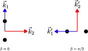
Figure 2: Two orientations of a diatomic molecule. The black circles indicate the nuclei. The scattering state depends on the relative angle between the molecular axis and the propagation direction $\vec{k}$ of the outgoing (asymptotically plane) wave. Therefore, while the states $|\vec{k}_{1}\rangle$ and $|\vec{k}_{1}^{\prime}\rangle$ satisfying $\vec{k}_{1}^{\mathrm{M}}=\vec{k}_{1}^{\prime\mathrm{M}}$ are related to each other by a simple rotation, the states $|\vec{k}_{1}\rangle$ and $|\vec{k}_{2}^{\prime}\rangle$ satisfying $\vec{k}_{1}^{\mathrm{L}}=\vec{k}_{2}^{\prime\mathrm{L}}$ are not related to each other in any simple way.

Now we will discuss two elementary applications of our methodology. First, we will derive the expression for the $b_{l,m}^{\left(1\right)}$ coefficients in one-photon ionization and discuss the molecular information they reveal. Afterwards we will derive and discuss the expressions for the $b_{0,0}^{\left(2\right)}$, $b_{1,0}^{\left(2\right)}$, and $b_{3,0}^{\left(2\right)}$ coefficients relevant for PECD in two-photon ionization. Note that the expressions for $b_{0,0}^{\left(1\right)}$ and $b_{1,0}^{\left(1\right)}$ coefficients in one-photon ionization and the $b_{1,0}^{\left(2\right)}$ coefficient in two-photon ionization have already been derived using a less general procedure in Ref. Ordonez and Smirnova (2018).

III The photoionization dipole field and the $b_{l,m}$ coefficients in one-photon ionization

For the field in Eq. (6), the first-order amplitude of the scattering state $|\vec{k}^{\mathrm{M}}\rangle$ reads as

$$a_{\vec{k}^{\mathrm{M}}}^{\left(1\right)}=A^{\left(1\right)}\left(\vec{D}^{\mathrm{L}}\cdot\vec{F}_{\omega_{L}}^{\mathrm{L}}\right),\qquad A^{\left(1\right)}=i\pi\delta_{\gamma}\left(\omega+\omega_{L}\right)$$ (11)

where we use the shorthand notations $\vec{D}^{\mathrm{M}}\equiv\vec{d}_{\vec{k}^{\mathrm{M}},0}^{\mathrm{M}}$, $\vec{F}^{\mathrm{L}}\equiv\vec{F}_{\omega_{L}}^{\mathrm{L}}$, and as usual $\vec{D}^{\mathrm{L}}=S\left(\varrho\right)\vec{D}^{\mathrm{M}}$. From here on, we must keep in mind that $\vec{D}^{\mathrm{M}}=\vec{D}^{\mathrm{M}}(\vec{k}^{\mathrm{M}})$ is a complex vector field that depends on $\vec{k}^{\mathrm{M}}$. That is, for a fixed initial state $|0\rangle$, $\vec{D}^{\mathrm{M}}(\vec{k}^{\mathrm{M}})$ is a mapping from the space of real three-dimensional vectors $\vec{k}^{\mathrm{M}}\in\mathbb{R}^{3}$ to the space of complex three-dimensional vectors $\vec{D}^{\mathrm{M}}\in\mathbb{C}^{3}$. From Eq. (11) it is clear that this complex vector field fully determines the response of the molecule to the ionizing field and therefore the coefficients $\tilde{b}_{l,m}^{\left(1\right)}$ must correspond to properties of this vector field. The question is: which property of the photoionization vector field $\vec{D}^{\mathrm{M}}(\vec{k}^{\mathrm{M}})$ is reflected in a given $\tilde{b}_{l,m}^{\left(1\right)}$ coefficient?

Since for first order amplitudes all frequencies act separately and the most general polarization of a single frequency is elliptical then we will assume an electric field that is elliptically polarized in the $xy$ plane with its major axis along either the $\hat{x}^{\mathrm{L}}$ or the $\hat{y}^{\mathrm{L}}$ axis. From symmetry it follows that the only non-zero $\tilde{b}_{l,m}^{\left(1\right)}$ coefficients are $b_{0,0}^{\left(1\right)}$, $b_{1,0}^{\left(1\right)}$, $b_{2,0}^{\left(1\right)}$, $\tilde{b}_{2,2}^{\left(1\right)}$, and $\tilde{b}_{2,-2}^{\left(1\right)}$ (we omit the tilde for $m=0$). With the help of Eqs. (5), (10), and performing the orientation integrals according to Ref. Andrews and Thirunamachandran (1977) we obtain (see Appendix)

$$b_{0,0}^{\left(1\right)}\left(k\right)=\left|A^{\left(1\right)}\right|^{2}\left\{\frac{1}{3\sqrt{4\pi}}\int\mathrm{d}\Omega_{k}^{\mathrm{M}}\left|\vec{D}^{\mathrm{M}}\right|^{2}\right\}\left\{\left|\vec{F}^{\mathrm{L}}\right|^{2}\right\},$$ (12)

$$b_{1,0}^{\left(1\right)}\left(k\right)=\left|A^{\left(1\right)}\right|^{2}\left\{\frac{1}{6}\sqrt{\frac{3}{4\pi}}\int\mathrm{d}\Omega_{k}^{\mathrm{M}}\left[\hat{k}^{\mathrm{M}}\cdot\left(\vec{D}^{\mathrm{M}*}\times\vec{D}^{\mathrm{M}}\right)\right]\right\}\left\{\hat{z}^{\mathrm{L}}\cdot\left(\vec{F}^{\mathrm{L}*}\times\vec{F}^{\mathrm{L}}\right)\right\},$$ (13)

$$b_{2,0}^{\left(1\right)}\left(k\right)=\left|A^{\left(1\right)}\right|^{2}\left\{\frac{1}{12\sqrt{5\pi}}\int\mathrm{d}\Omega_{k}^{\mathrm{M}}\left(3\left|\hat{k}^{\mathrm{M}}\cdot\vec{D}^{\mathrm{M}}\right|^{2}-\left|\vec{D}^{\mathrm{M}}\right|^{2}\right)\right\}\left\{3\left|\hat{z}^{\mathrm{L}}\cdot\vec{F}^{\mathrm{L}}\right|^{2}-\left|\vec{F}^{\mathrm{L}}\right|^{2}\right\},$$ (14)

$$\tilde{b}_{2,2}^{\left(1\right)}\left(k\right)=\left|A^{\left(1\right)}\right|^{2}\left\{\frac{1}{4\sqrt{15\pi}}\int\mathrm{d}\Omega_{k}^{\mathrm{M}}\left(3\left|\hat{k}^{\mathrm{M}}\cdot\vec{D}^{\mathrm{M}}\right|^{2}-\left|\vec{D}^{\mathrm{M}}\right|^{2}\right)\right\}\left\{\left|\hat{x}^{\mathrm{L}}\cdot\vec{F}^{\mathrm{L}}\right|^{2}-\left|\hat{y}^{\mathrm{L}}\cdot\vec{F}^{\mathrm{L}}\right|^{2}\right\},$$ (15)

and $\tilde{b}_{2,-2}^{\left(1\right)}=0$, a peculiarity of the one-photon case. That is, each $\tilde{b}_{l,m}^{\left(1\right)}$ coefficient is the product of: a coupling term $\left|A^{\left(1\right)}\right|^{2}$ depending on the energy level spacing of the molecule and the spectrum of the electric field, a molecular term expressed in the molecular frame and averaged over all $\hat{k}^{\mathrm{M}}$ directions, and a setup (field and laboratory axes) term expressed in the laboratory frame. Unlike the usual expressions for $\tilde{b}_{l,m}^{\left(1\right)}$ (see e.g. Ritchie (1976)), Eqs. (12)-(15) provide a rather simple expression for the molecular terms which, as we will now discuss, are simply related to concrete properties of the photoionization vector field $\vec{D}^{\mathrm{M}}$.

As expected, equation (12) shows that $b_{0,0}^{\left(1\right)}$, which is simply the total cross section, records only the $\hat{k}^{\mathrm{M}}$-averaged value of the magnitude of the field $\vec{D}^{\mathrm{M}}(\vec{k}^{\mathrm{M}})$. More interestingly, Eq. (13) shows that $b_{1,0}^{\left(1\right)}$ is sensitive to the $\hat{k}^{\mathrm{M}}$-averaged value of the triple product $\hat{k}^{\mathrm{M}}\cdot(\vec{D}^{\mathrm{M}*}\times\vec{D}^{\mathrm{M}})$, which, unlike $b_{0,0}^{\left(1\right)}$, depends on the angles between $\vec{k}^{\mathrm{M}}$, $\vec{D}^{\mathrm{M}}$, and $\vec{D}^{\mathrm{M}*}$. The meaning of this quantity can be made evident if we use an appropriate basis for our vector field $\vec{D}^{\mathrm{M}}$. Starting from the unit vectors in spherical coordinates $\hat{k}$, $\hat{\theta}_{k}$, and $\hat{\varphi}_{k}$ we define spherical vectors

$$\hat{k}_{\pm}^{\mathrm{M}}=\mp\frac{\hat{\theta}_{k}\mp i\hat{\varphi}_{k}}{\sqrt{2}}.$$ (16)

If we now write $\vec{D}^{\mathrm{M}}$ in terms of these contravariant helicity-basis vectors Varschalovich et al. (1988),

$$\vec{D}^{\mathrm{M}}=D_{+}^{\mathrm{M}}\hat{k}_{+}^{\mathrm{M}}+D_{-}^{\mathrm{M}}\hat{k}_{-}^{\mathrm{M}}+D_{k}^{\mathrm{M}}\hat{k}^{\mathrm{M}},$$ (17)

then

$$\hat{k}^{\mathrm{M}}\cdot\left(i\vec{D}^{\mathrm{M}*}\times\vec{D}^{\mathrm{M}}\right)=\left|D_{+}^{\mathrm{M}}\right|^{2}-\left|D_{-}^{\mathrm{M}}\right|^{2}.$$ (18)

The right hand side of Eq. (18) is analogous to the $s_{3}$ Stokes parameter for light waves in the circular polarization basis, which describes the difference in intensity between left and right circular polarization John David Jackson (1999). Here we identify the right hand side of Eq. (18) with the circular dichroism (CD) of the photoionization vector field $\vec{D}^{\mathrm{M}}$ in the direction $\hat{k}^{\mathrm{M}}$. Indeed, the right hand side of Eq. (18) is proportional to the difference between the probability of inducing the transition $\left|0\right\rangle\rightarrow|\vec{k}^{\mathrm{M}}\rangle$ using left and right circularly polarized light such that left ($+$) and right ($-$) rotations are defined with respect to $\hat{k}^{\mathrm{M}}$ (see Fig. 3). Therefore, the molecular term in $b_{1,0}^{\left(1\right)}$ is simply the $\hat{k}^{\mathrm{M}}$-averaged value of the $\vec{k}^{\mathrm{M}}$-specific CD in the molecular frame. Note that the $\vec{k}^{\mathrm{M}}$-specific CD can be non-zero even for achiral molecules, but its average over $\hat{k}^{\mathrm{M}}$ is only non-zero for chiral molecules. Further discussion of $b_{1,0}^{\left(1\right)}$ can be found in Ref. Ordonez and Smirnova (2019a). Remarkably, Eq. (18) shows that $b_{1,0}^{\left(1\right)}$ depends only on the tangential components of $\vec{D}^{\mathrm{M}}$, namely $D_{+}^{\mathrm{M}}$ and $D_{-}^{\mathrm{M}}$ (or equivalently $D_{\theta}^{\mathrm{M}}$ and $D_{\varphi}^{\mathrm{M}}$). Since the electric field term of $b_{1,0}^{\left(1\right)}$ has the same form as the molecular part we can apply a similar procedure and rewrite $b_{1,0}^{\left(1\right)}$ as

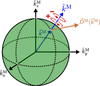
Figure 3: Sketch of the photoionization dipole $\vec{D}^{\mathrm{M}}(\vec{k}^{\mathrm{M}})\equiv\langle\vec{k}^{\mathrm{M}}|\vec{d}|0\rangle$ for a particular value of the photoelectron momentum $\vec{k}^{\mathrm{M}}$. Red circular arrows indicate the direction of left ($+$) and right ($-$) circular polarization with respect to $\hat{k}^{\mathrm{M}}$.

$$b_{1,0}^{\left(1\right)}=\left|A^{\left(1\right)}\right|^{2}\left\{\frac{1}{6}\sqrt{\frac{3}{4\pi}}\int\mathrm{d}\Omega_{k}^{\mathrm{M}}\left(\left|D_{+}^{\mathrm{M}}\right|^{2}-\left|D_{-}^{\mathrm{M}}\right|^{2}\right)\right\}\left\{\left|F_{+}^{\mathrm{L}}\right|^{2}-\left|F_{-}^{\mathrm{L}}\right|^{2}\right\}.$$ (19)

where

$$\vec{F}^{\mathrm{L}}=F_{+}^{\mathrm{L}}\hat{\epsilon}_{+}^{\mathrm{L}}+F_{-}^{\mathrm{L}}\hat{\epsilon}_{-}^{\mathrm{L}}+F_{0}^{\mathrm{L}}\hat{z}^{\mathrm{L}},$$ (20)

$$\hat{\epsilon}_{\pm}^{\mathrm{L}}=\frac{\hat{x}^{\mathrm{L}}\pm i\hat{y}^{\mathrm{L}}}{\sqrt{2}},$$ (21)

and $\left|F_{+}^{\mathrm{L}}\right|^{2}-\left|F_{-}^{\mathrm{L}}\right|^{2}$ is the Stokes parameter $s_{3}$ in the circular polarization basis John David Jackson (1999).

If we now take the ratio between $b_{1,0}^{\left(1\right)}$ [Eq. (19)] and $b_{0,0}^{\left(1\right)}$ [Eq. (12)] we get rid of the coupling term $|A^{\left(1\right)}|^{2}$, and therefore obtain an expression which factorizes into a purely molecular and a purely electric field part,

$$\beta_{1}^{\left(1\right)}\equiv\frac{\sqrt{3}b_{1,0}^{\left(1\right)}}{b_{0,0}^{\left(1\right)}}=\frac{3}{2}\left\{\frac{\int\mathrm{d}\Omega_{k}^{\mathrm{M}}\left(\left|D_{+}^{\mathrm{M}}\right|^{2}-\left|D_{-}^{\mathrm{M}}\right|^{2}\right)}{\int\mathrm{d}\Omega_{k}^{\mathrm{M}}\left|\vec{D}^{\mathrm{M}}\right|^{2}}\right\}\left\{\frac{\left|F_{+}^{\mathrm{L}}\right|^{2}-\left|F_{-}^{\mathrm{L}}\right|^{2}}{\left|\vec{F}^{\mathrm{L}}\right|^{2}}\right\}.$$ (22)

As discussed in Ref. Ordonez and Smirnova (2019b), for any number of photons $N$, we have that $\beta_{1}^{\left(N\right)}\equiv\sqrt{3}b_{1,0}^{\left(N\right)}/b_{0,0}^{\left(N\right)}=3j_{z}^{\left(N\right)}/j_{r}^{\left(N\right)}$, where $j_{z}^{\left(N\right)}$ is the net photoelectron current (i.e. vector sum of photoelectron currents in all directions) and $j_{r}^{\left(N\right)}$ is the total photoelectron current (i.e. sum of magnitudes of photoelectron currents in all directions). Equation (22) shows that the molecular factor is a measure of the degree of “circular polarization” of the photoionization vector field $\vec{D}^{\mathrm{M}}(\vec{k}^{\mathrm{M}})$ and takes values between $-1$ and $+1$, which correspond to the limits $\vec{D}^{\mathrm{M}}=D_{+}^{\mathrm{M}}\hat{k}_{+}^{\mathrm{M}}$ (left circularly polarized $\vec{D}^{\mathrm{M}}$) and $\vec{D}^{\mathrm{M}}=D_{-}^{\mathrm{M}}\hat{k}_{-}^{\mathrm{M}}$ (right circularly polarized $\vec{D}^{\mathrm{M}}$), respectively. Since the electric field factor is also a measure of the circular polarization of the electric field, then $\beta_{1}^{\left(1\right)}=3j_{z}^{\left(1\right)}/j_{r}^{\left(1\right)}$ is given by the product of the $\hat{k}^{\mathrm{M}}$-averaged “circular polarization” of the photoionization vector field $\vec{D}^{\mathrm{M}}(\vec{k}^{\mathrm{M}})$ and the circular polarization of the ionizing electric field. Clearly, for a known electric field, $\beta_{1}^{\left(1\right)}$ is a measure of the $\hat{k}^{\mathrm{M}}$-averaged “circular polarization” of $\vec{D}^{\mathrm{M}}(\vec{k}^{\mathrm{M}})$.

Moving on to the next coefficient, Eq. (14) shows that, complementarily to $b_{0,0}^{\left(1\right)}$ and $b_{1,0}^{\left(1\right)}$ which depend on the magnitude and on the tangential components of $\vec{D}^{\mathrm{M}}$, respectively, the coefficient $b_{2,0}^{\left(2\right)}$ depends on the projection of $\vec{D}^{\mathrm{M}}$ along $\hat{k}^{\mathrm{M}}$, i.e. on its radial component $D_{k}^{\mathrm{M}}$ [see Eq. (17))]. We can also consider the ratio between $b_{2,0}^{\left(2\right)}$ and $b_{1,0}^{\left(2\right)}$ to get rid of the coupling term, and obtain the asymmetry parameter,

$$\beta_{2}^{\left(1\right)}\equiv\frac{\sqrt{5}b_{2,0}^{\left(1\right)}\left(k\right)}{b_{0,0}^{\left(1\right)}\left(k\right)}=\frac{1}{2}\left\{3\frac{\int\mathrm{d}\Omega_{k}^{\mathrm{M}}\left|D_{k}^{\mathrm{M}}\right|^{2}}{\int\mathrm{d}\Omega_{k}^{\mathrm{M}}\left|\vec{D}^{\mathrm{M}}\right|^{2}}-1\right\}\left\{3\frac{\left|F_{z}^{\mathrm{L}}\right|^{2}}{\left|\vec{F}^{\mathrm{L}}\right|^{2}}-1\right\}.$$ (23)

which satisfies the well known fact that the values of $\beta_{2}^{\left(1\right)}$ for linear polarization along $z$ and circular polarization in the $xy$ plane are related to each other by a factor of -2 Reid (2003). More interestingly, we see that $\beta_{2}^{\left(1\right)}$ is a linear function of the molecular property

$$R\equiv\frac{\int\mathrm{d}\Omega_{k}^{\mathrm{M}}\left|D_{k}^{\mathrm{M}}\right|^{2}}{\int\mathrm{d}\Omega_{k}^{\mathrm{M}}\left|\vec{D}^{\mathrm{M}}\right|^{2}},\qquad 0\leq R\leq 1,$$ (24)

which measures to what extent the vector field $\vec{D}^{\mathrm{M}}(\vec{k}^{\mathrm{M}})$ is a radial field and takes values between $0$ and $1$, corresponding to the limits $\vec{D}^{\mathrm{M}}=D_{+}^{\mathrm{M}}\hat{k}_{+}^{\mathrm{M}}+D_{-}^{\mathrm{M}}\hat{k}_{-}^{\mathrm{M}}$ (tangential field) and $\vec{D}^{\mathrm{M}}=D_{k}^{\mathrm{M}}\hat{k}$ (radial field), respectively. Figure 4 shows $\beta_{2}^{\left(1\right)}$ as a function of $R$ for linear ($\vec{F}^{\mathrm{L}}=F_{z}\hat{z}^{\mathrm{L}}$) and circular polarization ($\vec{F}^{\mathrm{L}}=F_{\pm}\hat{\epsilon}_{\pm}$ ) along with the angular distributions obtained in the limits $R=0$ (tangential $\vec{D}^{\mathrm{M}}$) and $R=1$ (radial $\vec{D}^{\mathrm{M}}$). We can see that for both linearly and circularly polarized fields, a predominantly tangential field $\vec{D}^{\mathrm{M}}$ will yield most photoelectrons with directions perpendicular to the electric field, while a predominantly radial field $\vec{D}^{\mathrm{M}}$ will yield most photoelectrons with directions parallel to the electric field.

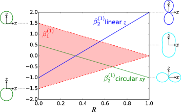
Figure 4: The relation between $\beta_{2}^{\left(1\right)}$ and the molecular property $R$, which measures how radial the photoionization dipole field $\vec{D}^{\mathrm{M}}(\vec{k}^{\mathrm{M}})=\langle\vec{k}^{\mathrm{M}}|\vec{d}^{\mathrm{M}}|0\rangle$ is in average for a given $k$ [see Eqs. (23) and (24)], for the case of linear polarization along $\hat{z}$ (thick blue line) and circular polarization in the $\hat{x}\hat{y}$ plane (narrow green line). The red shaded area shows the range of values that $\beta_{1}^{\left(1\right)}$ can take for a given value of $\beta_{2}^{\left(1\right)}$ (and correspondingly of $R$) for the circularly polarized case [see Eq. (25)]. $\beta_{1}^{\left(1\right)}$ is zero for linear polarization. The insets on the left show the angular distributions for the extreme values $\beta_{1}^{\left(1\right)}=\pm 1.5$ and $\beta_{2}^{\left(2\right)}=0.5$ obtained for circular polarization. The insets on the right show the angular distributions for $\beta_{1}^{\left(1\right)}=0$ (for simplicity) and $\beta_{2}^{\left(1\right)}=-1$ (bottom), $\beta_{2}^{\left(1\right)}=0.5$ (center), and $\beta_{2}^{\left(1\right)}=2$ (top), which are the values reached for linear and circular polarizations in the limits $R=0$ (tangential $\vec{D}^{\mathrm{M}}$) and $R=1$ (radial $\vec{D}^{\mathrm{M}}$).

Figure 4 also shows the range of values that $\beta_{1}^{\left(1\right)}$ can take as a function of $R$ for light circularly polarized in the $xy$ plane. This follows from using the expressions for $b_{0,0}^{\left(1\right)}$, $b_{1,0}^{\left(1\right)}$, and $b_{2,0}^{\left(1\right)}$ in Eqs. (12), (14), and (19), and taking into account that $|D_{+}|^{2}+|D_{-}|^{2}\geq|D_{+}|^{2}-|D_{-}|^{2}$, one can show that for circularly polarized light $\beta_{1}^{\left(1\right)}$ and $\beta_{2}^{\left(2\right)}$ satisfy the inequality (see Appendix)

$$|\beta_{1}^{\left(1\right)}|\leq 1+\beta_{2}^{\left(1\right)}.$$ (25)

This inequality follows naturally from the fact that, for circularly polarized light, small values of $\beta_{2}^{\left(1\right)}$ indicate that the field $\vec{D}(\vec{k})$ is (in average) mostly radial and therefore the tangential components along with $\beta_{1}^{\left(1\right)}$ are very small. On the contrary, big values of $\beta_{2}^{\left(1\right)}$ indicate that the field $\vec{D}(\vec{k})$ has (in average) a very small radial component, which means that the field is mostly tangential and can potentially display a large dichroism $|D_{+}|^{2}-|D_{-}|^{2}$. The maximal value of $|\beta_{1}^{\left(1\right)}|=3/2$ and occurs for $\beta_{2}^{\left(1\right)}=0.5$ [$\vec{D}(\vec{k})$ purely tangential]. As explained in Ref. Ordonez and Smirnova (2019b) [Eqs. (9) and (10)], the net photoelectron current [i.e. the vector sum of all photoelectron currents] is given by $j_{z}^{\mathrm{L}}(k)=\sqrt{4\pi/3}kb_{1,0}^{\left(1\right)}(k)$ and the total photoelectron current [i.e. the sum of the magnitudes of all photoelectron currents] is given by $j_{r}\left(k\right)=\sqrt{4\pi}kb_{0,0}^{\left(1\right)}(k)$. Therefore, the maximum value of the ratio of net photoelectron current to total current is $|j_{z}|/j_{r}=1/2$. Note that Eq. (25) can also be derived exclusively from the condition that the angular distribution $W^{\mathrm{L}}(\vec{k}^{\mathrm{L}})$ [Eq. (2)] is positive for every $\vec{k}^{\mathrm{L}}$.

Finally, Eq. (15) shows that, up to constants, $\tilde{b}_{2,2}^{\left(1\right)}$ differs from $b_{2,0}^{\left(1\right)}$ only in the electric field factor, which in the case of $\tilde{b}_{2,2}^{\left(1\right)}$ yields the $s_{1}$ Stokes parameter in the linear polarization basis John David Jackson (1999). That is, $\tilde{b}_{2,2}^{\left(1\right)}$ and $b_{2,0}^{\left(1\right)}$ reveal the same information about the photoionization vector field $\vec{D}^{\mathrm{M}}(\vec{k}^{\mathrm{M}})$ and differ only on the electric field information they encode. This is a general property of $\tilde{b}_{l,m}$ coefficients with the same value of $l$ and corresponding to the same quantum pathway. It reflects the fact that such coefficients differ only in their laboratory axes vectors [see e.g. Eqs. (9) and (10)] but not on their molecular vectors (photoelectron momentum and transition dipoles), and therefore they involve the same molecular rotational invariants.

IV PECD in resonantly enhanced two-photon ionization

We begin by rewriting Eq. (9) as

$$\tilde{b}_{l,m}^{\left(2\right)}\left(k\right)=\frac{1}{2}|A^{\left(2\right)}|^{2}d^{2}\left|F\right|^{2}\int\mathrm{d}\Omega_{k}^{\mathrm{M}}\int\mathrm{d}\varrho\,\tilde{Y}_{l}^{m}(\hat{k}^{\mathrm{L}})\sin^{2}\beta|\vec{D}^{\mathrm{L}}\cdot\vec{F}^{\mathrm{L}}|^{2}.$$ (26)

where we used the shorthand notation $\vec{D}^{\mathrm{M}}\equiv\vec{d}_{\vec{k}^{\mathrm{M}},1}^{\mathrm{M}}$ for the photoionization dipole from the intermediate state, $\vec{F}^{\mathrm{L}}\equiv\vec{F}_{\omega_{L}}^{\mathrm{L}}=F\left(1,i\sigma,0\right)/\sqrt{2}$, $\sigma=\pm 1$, and we chose the molecular axis so that $\vec{d}^{\mathrm{M}}\equiv\vec{d}_{1,0}^{\mathrm{M}}=d\hat{z}^{\mathrm{M}}$ and therefore $\vec{d}^{\mathrm{L}}=d(\sin\beta\cos\alpha,$$\sin\beta\sin\alpha$$,\cos\beta)$ where $\alpha\beta\gamma$ are the Euler angles in the $ZYZ$ convention, and in particular $\beta$ is the angle between the molecular and laboratory $\hat{z}$ axes. This yields $|\vec{d}^{\mathrm{L}}\cdot\vec{F}^{\mathrm{L}}|^{2}=\frac{1}{2}d^{2}\left|F\right|^{2}\sin^{2}\beta$. Written like this, the second order coefficients $\tilde{b}_{l,m}^{\left(2\right)}\left(k\right)$ take the form of the first order coefficients $\tilde{b}_{l,m}^{\left(1\right)}$ for an anisotropic (in this case anti-aligned) sample with an orientation distribution given by $w\left(\beta\right)\propto\sin^{2}\beta$ and an initial state $\left|1\right\rangle$ instead of $\left|0\right\rangle$ (see also Refs. Ordonez and Smirnova (2019a); Lehmann et al. (2013); Goetz et al. (2017)). Such anisotropy gives a certain preference to the $z$ components of the molecular vectors. Performing the orientation averaging according to Ref. Andrews and Thirunamachandran (1977), the expressions for the total absorption $b_{0,0}^{\left(2\right)}$, and for the enantiosensitive terms $b_{1,0}^{\left(2\right)}$ and $b_{3,0}^{\left(2\right)}$ yield (see Appendix)

$$b_{0,0}^{\left(2\right)} =C\left\{\frac{1}{3}\frac{1}{\sqrt{4\pi}}\int\mathrm{d}\Omega_{k}^{\mathrm{M}}|D_{\mathrm{eff(0,0)}}^{\mathrm{M}}|^{2}\right\},$$ (27)

$$b_{1,0}^{\left(2\right)} =\sigma C\left\{\frac{1}{6}\sqrt{\frac{3}{4\pi}}\int\mathrm{d}\Omega_{k}^{\mathrm{M}}\left[\hat{k}^{\mathrm{M}}\cdot\left(i\vec{D}_{\mathrm{eff}\left(1,0\right)}^{\mathrm{M}*}\times\vec{D}_{\mathrm{eff}\left(1,0\right)}^{\mathrm{M}}\right)\right]\right\},$$ (28)

$$=\sigma C\left\{\frac{1}{6}\sqrt{\frac{3}{4\pi}}\int\mathrm{d}\Omega_{k}^{\mathrm{M}}\left[\vec{K}_{1,0}^{\mathrm{M}}\cdot\left(i\vec{D}^{\mathrm{M}*}\times\vec{D}^{\mathrm{M}}\right)\right]\right\}\frac{1}{5}\sqrt{\frac{17}{5}},$$ (29)

$$b_{3,0}^{\left(2\right)} =\sigma C\left\{\frac{1}{35\sqrt{3}}\sqrt{\frac{7}{16\pi}}\int\mathrm{d}\Omega_{k}^{\mathrm{M}}\left[\vec{K}_{3,0}^{\mathrm{M}}\cdot\left(i\vec{D}^{\mathrm{M}*}\times\vec{D}^{\mathrm{M}}\right)\right]\right\},$$ (30)

where $C\equiv d^{2}\left|F\right|^{4}|A^{\left(2\right)}|^{2}$ is a common factor to all $b_{l,m}^{\left(2\right)}$ coefficients that simply encodes the bound-bound transition and the second order character of the process, and the expressions for $\vec{D}_{\mathrm{eff}\left(0,0\right)}^{\mathrm{M}}$, $\vec{D}_{\mathrm{eff}\left(1,0\right)}^{\mathrm{M}}$, $\vec{K}_{1,0}^{\mathrm{M}}$, and $\vec{K}_{3,0}^{\mathrm{M}}$ are given below. We wrote Eqs. (27)-(30) so that we can draw a parallel to the corresponding Eqs. (12) and (13) in the one-photon case. Equations (27) and (28) show that we can recover the forms obtained in the one-photon case if we introduce effectively stretched photoionization dipoles given by

$$\vec{D}_{\mathrm{eff}\left(0,0\right)}^{\mathrm{M}}\equiv\sqrt{\frac{3}{10}}\left(D_{x}^{\mathrm{M}},D_{y}^{\mathrm{M}},\frac{2}{\sqrt{3}}D_{z}^{\mathrm{M}}\right),$$ (31)

and

$$\vec{D}_{\mathrm{eff}\left(1,0\right)}^{\mathrm{M}}\equiv\frac{1}{\sqrt{5}}\left(D_{x}^{\mathrm{M}},D_{y}^{\mathrm{M}},2D_{z}^{\mathrm{M}}\right).$$ (32)

In view of the discussion in Sec. III, Eq. (27) shows that $b_{0,0}^{\left(2\right)}$ records the $\hat{k}^{\mathrm{M}}$-averaged magnitude of an effective photoionization dipole $\vec{D}_{\mathrm{eff}\left(0,0\right)}^{\mathrm{M}}(\vec{k}^{\mathrm{M}})$. Similarly, Eq. (28) shows that $b_{1,0}^{\left(2\right)}$ records the “circular polarization” [see Eq. (18)] or equivalently the $\vec{k}^{\mathrm{M}}$-averaged value of the $\vec{k}^{\mathrm{M}}$-specific CD of an effective photoionization dipole $\vec{D}_{\mathrm{eff}\left(1,0\right)}^{\mathrm{M}}(\vec{k}^{\mathrm{M}})$. Their ratio, $\beta_{1}^{\left(2\right)}\equiv\sqrt{3}b_{1,0}^{\left(2\right)}/b_{0,0}^{\left(2\right)}$, can be interpreted as the average “circular polarization” of $\vec{D}_{\mathrm{eff}\left(1,0\right)}^{\mathrm{M}}$ normalized with respect to the average magnitude of $\vec{D}_{\mathrm{eff}\left(0,0\right)}^{\mathrm{M}}$.

In the case of $b_{3,0}^{\left(2\right)}$, quadratic terms in $k_{z}$ (see Appendix) hinder a straightforward interpretation of the integrand in terms of a effectively stretched $\vec{D}^{\mathrm{M}}$. However, like $b_{1,0}^{\left(1\right)}$ and $b_{1,0}^{\left(2\right)}$ [Eqs. (13) and (29)], Eq. (30) shows that $b_{3,0}^{\left(2\right)}$ depends on the photoionization dipole $\vec{D}^{\mathrm{M}}(\vec{k}^{\mathrm{M}})$ only through the $\vec{k}^{\mathrm{M}}$-dependent field

$$\vec{B}^{\mathrm{M}}\equiv i\vec{D}^{\mathrm{M}*}\times\vec{D}^{\mathrm{M}},$$ (33)

and we can therefore attempt an interpretation of $b_{3,0}^{\left(2\right)}$ in terms of $\vec{B}^{\mathrm{M}}$ directly.

We have already found rigorous physical interpretations for the projections $\hat{A}^{\mathrm{M}}\cdot\vec{B}^{\mathrm{M}}$ for $\hat{A}^{\mathrm{M}}=\hat{x}^{\mathrm{M}},\hat{y}^{\mathrm{M}},\hat{z}^{\mathrm{M}},\hat{k}^{\mathrm{M}}$ (see Ordonez and Smirnova (2019a) and Sec. III). In these cases we found that $\hat{A}^{\mathrm{M}}\cdot\vec{B}^{\mathrm{M}}$ yields the $\hat{k}^{\mathrm{M}}$-specific CD associated to the transition $\left|0\right\rangle\rightarrow|\vec{k}^{\mathrm{M}}\rangle$ for light circularly polarized with respect to the axis $\hat{A}^{\mathrm{M}}$ (see Fig. 3). In fact, this interpretation is valid for an arbitrary $\hat{A}^{\mathrm{M}}$. To see this, note that for a given $\hat{A}^{\mathrm{M}}$ one can always build $\hat{A}^{\mathrm{M}}$-dependent unit vectors $\hat{e}_{\pm}^{\mathrm{M}}$ associated to positive and negative rotations around $\hat{A}^{\mathrm{M}}$, write $\vec{D}^{\mathrm{M}}=D_{+}^{\mathrm{M}}\hat{e}_{+}^{\mathrm{M}}+D_{-}^{\mathrm{M}}\hat{e}_{-}^{\mathrm{M}}+D_{0}^{\mathrm{M}}\hat{A}^{\mathrm{M}}$ and obtain $\hat{A}^{\mathrm{M}}\cdot\vec{B}^{\mathrm{M}}=|\vec{D}_{+}^{\mathrm{M}}|^{2}-|\vec{D}_{-}^{\mathrm{M}}|^{2}$. This scalar product is evidently maximized for $\hat{A}^{\mathrm{M}}=\hat{B}^{\mathrm{M}}$, and therefore the direction of $\vec{B}^{\mathrm{M}}$ indicates the axis with respect to which the $\hat{k}^{\mathrm{M}}$-specific CD is maximal. The magnitude of $\vec{B}^{\mathrm{M}}$ is then the magnitude of such maximal $\hat{k}^{\mathrm{M}}$-specific CD. Light circularly polarized with respect to axes perpendicular to $\vec{B}^{\mathrm{M}}$ yield zero $\hat{k}^{\mathrm{M}}$-specific CD.

While Eq. (13) shows that $b_{1,0}^{\left(1\right)}$ involves the projection of $\vec{B}^{\mathrm{M}}$ on the radial vector $\hat{k}^{\mathrm{M}}$, Eqs. (29) and (30) show that $b_{1,0}^{\left(2\right)}$ and $b_{3,0}^{\left(2\right)}$ involve the projection of $\vec{B}^{\mathrm{M}}$ on the vector fields $\vec{K}_{1,0}^{\mathrm{M}}$ and $\vec{K}_{3,0}^{\mathrm{M}}$, respectively, defined as (see Appendix)

$$\vec{K}_{1,0}^{\mathrm{M}}\equiv\sqrt{\frac{5}{17}}\left(2\hat{k}^{\mathrm{M}}-\frac{k_{z}^{\mathrm{M}}}{k}\hat{z}^{\mathrm{M}}\right),$$ (34)

$$\vec{K}_{3,0}^{\mathrm{M}}\equiv\frac{\sqrt{3}}{2}\left\{\left[1-5\left(\frac{k_{z}^{\mathrm{M}}}{k}\right)^{2}\right]\hat{k}^{\mathrm{M}}+2\frac{k_{z}^{\mathrm{M}}}{k}\hat{z}^{\mathrm{M}}\right\},$$ (35)

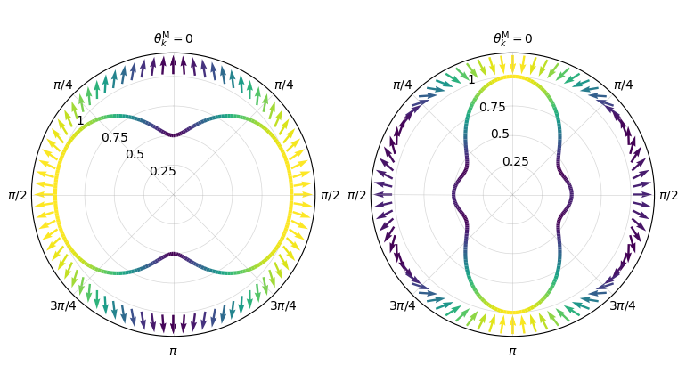
Figure 5: Direction (arrows) and magnitude (color and solid lines) of the vector fields $\vec{K}_{1,0}^{\mathrm{M}}(\hat{k}^{\mathrm{M}})$ and $\vec{K}_{3,0}^{\mathrm{M}}(\hat{k}^{\mathrm{M}})$ in Eqs. (34) and (35).

and shown in Fig. 5 as a function of $\theta_{k}^{\mathrm{M}}$ on a plane parallel to $k_{z}^{\mathrm{M}}$. The integrations over all $\hat{k}^{\mathrm{M}}$ directions in Eqs. (28) and (30) tell us that $b_{1,0}^{\left(2\right)}$ and $b_{3,0}^{\left(2\right)}$ record the extent to which the vector field $\vec{B}^{\mathrm{M}}$ resembles the vector fields $\vec{K}_{1,0}^{\mathrm{M}}$ and $\vec{K}_{3,0}^{\mathrm{M}}$, respectively, and therefore record structural information about $\vec{B}^{\mathrm{M}}$. Such information can be made more explicit by expanding $\vec{K}_{1,0}^{\mathrm{M}}$, $\vec{K}_{3,0}^{\mathrm{M}}$, and $\vec{B}^{\mathrm{M}}$ in terms of vector spherical harmonics Barrera et al. (1985) $\vec{Y}_{l,m}^{\mathrm{M}}(\hat{k}^{\mathrm{M}})\equiv Y_{l}^{m}(\hat{k}^{\mathrm{M}})\hat{k}^{\mathrm{M}}$, $\vec{\Psi}_{l,m}^{\mathrm{M}}(\hat{k}^{\mathrm{M}})\equiv k\vec{\nabla}Y_{l,m}(\hat{k}^{\mathrm{M}})/\sqrt{l\left(l+1\right)}$, and $\vec{\Phi}_{l,m}^{\mathrm{M}}(\hat{k}^{\mathrm{M}})\equiv\hat{k}^{\mathrm{M}}\times\vec{\Psi}_{l,m}^{\mathrm{M}}/\sqrt{l\left(l+1\right)}$,

$$\vec{K}_{1,0}^{\mathrm{M}}(\hat{k}^{\mathrm{M}})=\frac{2}{3}\sqrt{\frac{\pi}{17}}\left[5\sqrt{5}\vec{Y}_{0,0}^{\mathrm{M}}(\hat{k}^{\mathrm{M}})-2\vec{Y}_{2,0}^{\mathrm{M}}(\hat{k}^{\mathrm{M}})-\sqrt{6}\vec{\Psi}_{2,0}^{\mathrm{M}}(\hat{k}^{\mathrm{M}})\right],$$ (36)

$$\vec{K}_{3,0}^{\mathrm{M}}(\hat{k}^{\mathrm{M}})=2\sqrt{\frac{\pi}{5}}\left[-\sqrt{3}\vec{Y}_{2,0}^{\mathrm{M}}(\hat{k}^{\mathrm{M}})+\sqrt{2}\vec{\Psi}_{2,0}^{\mathrm{M}}(\hat{k}^{\mathrm{M}})\right],$$ (37)

$$\vec{B}^{\mathrm{M}}(\vec{k}^{\mathrm{M}})=\sum_{l,m}\left[\mathcal{B}_{l,m}^{Y}(k)\vec{Y}_{l,m}^{\mathrm{M}}(\hat{k}^{\mathrm{M}})+\mathcal{B}_{l,m}^{\Psi}(k)\vec{\Psi}_{l,m}^{\mathrm{M}}(\hat{k}^{\mathrm{M}})+\mathcal{B}_{l,m}^{\Phi}(k)\vec{\Phi}_{l,m}^{\mathrm{M}}(\hat{k}^{\mathrm{M}})\right].$$ (38)

Replacing Eqs. (33), (36)-(38) in Eqs. (29) and (30) and using the orthonormality relations for the vector spherical harmonics Barrera et al. (1985), we obtain

$$b_{1,0}^{\left(2\right)}=\frac{\sigma C}{30\sqrt{15}}\left(5\sqrt{5}\mathcal{B}_{0,0}^{Y}-2\mathcal{B}_{2,0}^{Y}-\sqrt{6}\mathcal{B}_{2,0}^{\Psi}\right),$$ (39)

$$b_{3,0}^{\left(2\right)}=\frac{\sigma C}{10\sqrt{105}}\left(-\sqrt{3}\mathcal{B}_{2,0}^{Y}+\sqrt{2}\mathcal{B}_{2,0}^{\Psi}\right).$$ (40)

That is, while in the one-photon case $b_{1,0}^{\left(1\right)}$ encodes $\mathcal{B}_{0,0}^{Y}$ (because $\hat{k}^{\mathrm{M}}\propto\vec{Y}_{0,0}^{\mathrm{M}}$), in the two-photon case $b_{1,0}^{\left(2\right)}$ and $b_{3,0}^{\left(2\right)}$ encode $\mathcal{B}_{0,0}^{Y}$, $\mathcal{B}_{2,0}^{Y}$, and $\mathcal{B}_{2,0}^{\Psi}$. This motivates looking for a third linearly independent equation to solve for $\mathcal{B}_{0,0}^{Y}$, $\mathcal{B}_{2,0}^{Y}$, and $\mathcal{B}_{2,0}^{\Psi}$. This is delivered by the equation for $b_{1,0}^{\prime\left(2\right)}$ for the complementary process where the first photon is linearly polarized along $\hat{z}^{\mathrm{L}}$ and the second photon is circularly polarized in the $\hat{x}^{\mathrm{L}}\hat{y}^{\mathrm{L}}$ plane (see Appendix),

$$b_{1,0}^{\prime\left(2\right)}=\frac{\sigma C}{30\sqrt{15}}\left(5\sqrt{5}\mathcal{B}_{0,0}^{Y}+4\mathcal{B}_{2,0}^{Y}+2\sqrt{6}\mathcal{B}_{2,0}^{\Psi}\right).$$ (41)

Equation (41) together with (39) and (40) yield

$$\mathcal{B}_{0,0}^{Y}=\frac{2\sqrt{3}}{\sigma C}\left(2b_{1,0}^{\left(2\right)}+b_{1,0}^{\prime\left(2\right)}\right),$$ (42)

$$\mathcal{B}_{2,0}^{Y}=\frac{2\sqrt{15}}{\sigma C}\left(-b_{1,0}^{\left(2\right)}-\sqrt{21}b_{3,0}^{\left(2\right)}+b_{1,0}^{\prime\left(2\right)}\right),$$ (43)

$$\mathcal{B}_{2,0}^{\Psi}=\frac{\sqrt{30}}{\sigma C}\left(-\sqrt{3}b_{1,0}^{\left(2\right)}+2\sqrt{7}b_{3,0}^{\left(2\right)}+\sqrt{3}b_{1,0}^{\prime\left(2\right)}\right).$$ (44)

These coefficients quantify the contributions of the fields $\vec{Y}_{0,0}^{\mathrm{M}}(\hat{k}^{\mathrm{M}})$$\propto$$\hat{k}^{\mathrm{M}}$, $\vec{Y}_{2,0}^{\mathrm{M}}(\hat{k}^{\mathrm{M}})$$\propto$$(3\cos^{2}\theta_{k}^{\mathrm{M}}$$-1)\hat{k}^{\mathrm{M}}$, and $\vec{\Psi}_{2,0}^{\mathrm{M}}(\hat{k}^{\mathrm{M}})$$\propto$$-\cos\theta_{k}^{\mathrm{M}}$$\sin\theta_{k}^{\mathrm{M}}\hat{\theta}_{k}^{\mathrm{M}}$ to the total field $\vec{B}^{\mathrm{M}}(\hat{k}^{\mathrm{M}})$ [Eq. (33)]. Equations (42)-(44) thus clearly show how structural information of the molecular field $\vec{B}^{\mathrm{M}}(\vec{k}^{\mathrm{M}})$ can be reconstructed from photoelectron angular distributions resulting from an initially isotropic sample of chiral molecules.

V Conclusions

We have presented an alternative approach to obtain expressions for the $b_{l,m}^{\left(N\right)}$ coefficients of photoelectron angular distributions resulting from perturbative $N$-photon ionization of isotropic samples. These expressions are explicitly written in terms of products between the molecular rotational invariants and the setup rotational invariants, and do not invoke a partial wave expansion for the scattering wave function. The molecular rotational invariants are expressed in terms of vector products involving only molecular vectors: transition dipoles and the photoelectron momentum labeling a particular scattering state in the molecular frame. The setup rotational invariants are expressed in terms of vector products involving only setup vectors: field polarization vectors and detection axes. Our expressions reveal the coupling of molecular and setup rotational invariants. Knowledge of this coupling can assist the interpretation and design of future experiments and simulations. The standard expressions can be recovered by subsequent expansion of the scattering wave function if needed.

With the help of this methodology we found that, independently of the polarization of the field, enantiosensitive $b_{l,m}^{\left(N_{1},N_{2}\right)}$ coefficients resulting from interference between pathways involving $N_{1}$ and $N_{2}$ photons have odd $l+N_{1}+N_{2}$.

The application of our methodology to the case of one-photon ionization $|0\rangle$$\rightarrow$$|\vec{k}\rangle$ reveals a clear meaning for the molecular information encoded in each of the $b_{l,m}^{\left(1\right)}$ coefficients which is otherwise obscured in the usual (and equivalent) formulation in terms of partial waves: $b_{0,0}^{\left(1\right)}$ encodes the average magnitude of the photoionization dipole $\vec{D}(\vec{k})\equiv\langle\vec{k}|\vec{d}|0\rangle$; $b_{1,0}^{\left(1\right)}$ encodes the average radial component of the propensity field $\vec{B}\equiv i\vec{D}^{*}\times\vec{D},$ which in turn encodes the average circular dichroism of $\vec{D}(\vec{k})$ and depends only on its transverse components; and $b_{2,0}^{\left(1\right)}$ encodes the average radial component of $\vec{D}(\vec{k})$. The averages are taken with respect to the direction of the photoelectron momentum $\vec{k}$ in the molecular frame. $b_{1,0}^{\left(1\right)}$ is sensitive to a single coefficient of the vector spherical harmonic expansion of $\vec{B}(\vec{k})$.

We also derived expressions for the coefficients $b_{0,0}^{\left(2\right)}$, $b_{1,0}^{\left(2\right)}$, and $b_{3,0}^{\left(2\right)}$ relevant for two-photon resonantly enhanced ionization $|0\rangle$$\rightarrow$$|1\rangle$$\rightarrow$$|\vec{k}\rangle$ of isotropic chiral samples with circularly polarized light. The coefficients $b_{0,0}^{\left(2\right)}$ and $b_{1,0}^{\left(2\right)}$ have analogous interpretations to those found in the one-photon case provided one takes into account an effective anisotropic stretching of the photoionization dipoles. $b_{1,0}^{\left(2\right)}$ and $b_{3,0}^{\left(2\right)}$ yield structural information about the propensity field $\vec{B}\equiv i\vec{D}^{*}\times\vec{D}$ Ordonez and Smirnova (2019a), which encodes the $\vec{k}$-specific circular dichroism. In particular they depend only on three coefficients of the vector spherical harmonic expansion of $\vec{B}(\vec{k})$. These coefficients can be solved for in terms of $b_{1,0}^{\left(2\right)}$, $b_{3,0}^{\left(2\right)}$, and $b_{1,0}^{\prime\left(2\right)}$, where the latter corresponds to the process where the first photon is linearly polarized.

Further application of the methodology introduced here can be found in the companion paper Ordonez and Smirnova , where it is used to analyze the enantiosensitive asymmetry recently found in the photoelectron angular distributions resulting from interaction of chiral samples with a field containing $\omega$ and $2\omega$ frequencies linearly polarized orthogonal to each other Demekhin et al. (2018); Demekhin (2019).

VI Appendix

VI.1 Real spherical harmonics

The real spherical harmonics (with tilde) are defined in terms of the complex spherical harmonics (without tilde) according to

$$\tilde{Y}_{l}^{m}=\begin{cases}\sqrt{2}\left(-1\right)^{m}\mathrm{Im}\left\{Y_{l}^{\left|m\right|}\right\},&m<0,\\ Y_{l}^{0}&m=0,\\ \sqrt{2}\left(-1\right)^{m}\mathrm{Re}\left\{Y_{l}^{\left|m\right|}\right\},&m>0,\end{cases}$$ (45)

and satisfy the orthonormality relation

$$\int\mathrm{d}\Omega\,\tilde{Y}_{l}^{m}\tilde{Y}_{\lambda}^{\mu}=\delta_{l,\lambda}\delta_{m,\mu}.$$ (46)

For an arbitrary function $W$, the relation between the coefficients of the real and the complex spherical harmonics can be derived from

$$W=\sum_{l,m}b_{l,m}Y_{l}^{m}=\sum_{l}\left\{\tilde{b}_{l,0}\tilde{Y}_{l}^{0}+\sum_{\left|m\right|=1}^{l}\left[\tilde{b}_{l,\left|m\right|}Y_{l}^{\left|m\right|}+b_{l,-\left|m\right|}Y_{l}^{-\left|m\right|}\right]\right\},$$ (47)

and yields

$$\tilde{b}_{l,m}=\begin{cases}-\left(-1\right)^{m}\sqrt{2}\mathrm{Im}\left\{b_{l,\left|m\right|}\right\},&m<0,\\ b_{l,m},&m=0,\\ \left(-1\right)^{m}\sqrt{2}\mathrm{Re}\left\{b_{l,m}\right\},&m>0.\end{cases}$$ (48)

VI.2 Derivation of the $\boldsymbol{\tilde{b}_{l,m}}$ coefficients in one-photon-ionization

According to Eqs. (5), (6), and (11), and following Ref. Andrews and Thirunamachandran (1977) for the orientation averaging, we obtain

$$b_{0,0}^{\left(1\right)} =\left|A^{\left(1\right)}\right|^{2}\int\mathrm{d}\Omega_{k}^{\mathrm{M}}\int\mathrm{d}\varrho\,Y_{0}^{0}(\hat{k}^{\mathrm{L}})\left(\vec{D}^{\mathrm{L}*}\cdot\vec{F}^{\mathrm{L}*}\right)\left(\vec{D}^{\mathrm{L}}\cdot\vec{F}^{\mathrm{L}}\right),$$

$$=\frac{\left|A^{\left(1\right)}\right|^{2}}{\sqrt{4\pi}}\int\mathrm{d}\Omega_{k}^{\mathrm{M}}\int\mathrm{d}\varrho\,\left(\vec{D}^{\mathrm{L}*}\cdot\vec{F}^{\mathrm{L}*}\right)\left(\vec{D}^{\mathrm{L}}\cdot\vec{F}^{\mathrm{L}}\right),$$

$$=\frac{\left|A^{\left(1\right)}\right|^{2}}{3\sqrt{4\pi}}\int\mathrm{d}\Omega_{k}^{\mathrm{M}}\left|\vec{D}^{\mathrm{M}}\right|^{2}\left|\vec{F}^{\mathrm{L}}\right|^{2}.$$ (49)

$$b_{1,0}^{\left(1\right)} =\left|A^{\left(1\right)}\right|^{2}\int\mathrm{d}\Omega_{k}^{\mathrm{M}}\int\mathrm{d}\varrho\,Y_{1}^{0}(\hat{k}^{\mathrm{L}})\left(\vec{D}^{\mathrm{L}*}\cdot\vec{F}^{\mathrm{L}*}\right)\left(\vec{D}^{\mathrm{L}}\cdot\vec{F}^{\mathrm{L}}\right),$$

$$=\left|A^{\left(1\right)}\right|^{2}\sqrt{\frac{3}{4\pi}}\int\mathrm{d}\Omega_{k}^{\mathrm{M}}\int\mathrm{d}\varrho\,\left(\hat{k}^{\mathrm{L}}\cdot\hat{z}^{\mathrm{L}}\right)\left(\vec{D}^{\mathrm{L}*}\cdot\vec{F}^{\mathrm{L}*}\right)\left(\vec{D}^{\mathrm{L}}\cdot\vec{F}^{\mathrm{L}}\right),$$

$$=\left|A^{\left(1\right)}\right|^{2}\frac{1}{6}\sqrt{\frac{3}{4\pi}}\int\mathrm{d}\Omega_{k}^{\mathrm{M}}\left[\hat{k}^{\mathrm{M}}\cdot\left(\vec{D}^{\mathrm{M}*}\times\vec{D}^{\mathrm{M}}\right)\right]\left[\hat{z}^{\mathrm{L}}\cdot\left(\vec{F}^{\mathrm{L}*}\times\vec{F}^{\mathrm{L}}\right)\right].$$ (50)

$$b_{2,0}^{\left(1\right)} =\left|A^{\left(1\right)}\right|^{2}\int\mathrm{d}\Omega_{k}^{\mathrm{M}}\int\mathrm{d}\varrho\,Y_{2}^{0}(\hat{k}^{\mathrm{L}})\left(\vec{D}^{\mathrm{L}*}\cdot\vec{F}^{\mathrm{L}*}\right)\left(\vec{D}^{\mathrm{L}}\cdot\vec{F}^{\mathrm{L}}\right),$$

$$=\left|A^{\left(1\right)}\right|^{2}\frac{1}{4}\sqrt{\frac{5}{\pi}}\int\mathrm{d}\Omega_{k}^{\mathrm{M}}\int\mathrm{d}\varrho\,\left[3\left(\hat{k}^{\mathrm{L}}\cdot\hat{z}^{\mathrm{L}}\right)^{2}-1\right]\left(\vec{D}^{\mathrm{L}*}\cdot\vec{F}^{\mathrm{L}*}\right)\left(\vec{D}^{\mathrm{L}}\cdot\vec{F}^{\mathrm{L}}\right)$$

$$=\left|A^{\left(1\right)}\right|^{2}\frac{3}{4}\sqrt{\frac{5}{\pi}}\int\mathrm{d}\Omega_{k}^{\mathrm{M}}\int\mathrm{d}\varrho\,\left(\hat{k}^{\mathrm{L}}\cdot\hat{z}^{\mathrm{L}}\right)^{2}\left(\vec{D}^{\mathrm{L}*}\cdot\vec{F}^{\mathrm{L}*}\right)\left(\vec{D}^{\mathrm{L}}\cdot\vec{F}^{\mathrm{L}}\right)-\sqrt{\frac{5}{4}}b_{0,0}^{\left(1\right)},$$ (51)

For the remaining integral over orientations in $b_{2,0}^{\left(1\right)}$ we have

$$\int\mathrm{d}\varrho\,\left(\hat{k}^{\mathrm{L}}\cdot\hat{z}^{\mathrm{L}}\right)^{2}\left(\vec{D}^{\mathrm{L}*}\cdot\vec{F}^{\mathrm{L}*}\right)\left(\vec{D}^{\mathrm{L}}\cdot\vec{F}^{\mathrm{L}}\right) =\vec{g}^{\left(4\right)}\cdot M^{\left(4\right)}\vec{f}^{\left(4\right)}$$ (52)

where

$$\vec{g}^{\left(4\right)}=\left[\begin{array}[]{c}(\hat{k}^{\mathrm{M}}\cdot\vec{k}^{\mathrm{M}})(\vec{D}^{\mathrm{M}*}\cdot\vec{D}^{\mathrm{M}})\\ (\hat{k}^{\mathrm{M}}\cdot\vec{D}^{\mathrm{M}*})(\hat{k}^{\mathrm{M}}\cdot\vec{D}^{\mathrm{M}})\\ (\hat{k}^{\mathrm{M}}\cdot\vec{D}^{\mathrm{M}})(\hat{k}^{\mathrm{M}}\cdot\vec{D}^{\mathrm{M}*})\end{array}\right]=\left[\begin{array}[]{c}|\vec{D}^{\mathrm{M}}|^{2}\\ |\hat{k}^{\mathrm{M}}\cdot\vec{D}^{\mathrm{M}}|^{2}\\ |\hat{k}^{\mathrm{M}}\cdot\vec{D}^{\mathrm{M}}|^{2}\end{array}\right]$$ (53)

$$M^{\left(4\right)}=\frac{1}{30}\left[\begin{array}[]{ccc}4&-1&-1\\ -1&4&-1\\ -1&-1&4\end{array}\right]$$ (54)

$$\vec{f}^{\left(4\right)}=\left[\begin{array}[]{c}\left(\hat{z}^{\mathrm{L}}\cdot\hat{z}^{\mathrm{L}}\right)(\vec{F}^{\mathrm{L}*}\cdot\vec{F}^{\mathrm{L}})\\ (\hat{z}^{\mathrm{L}}\cdot\vec{F}^{\mathrm{L}*})(\hat{z}^{\mathrm{L}}\cdot\vec{F}^{\mathrm{L}})\\ (\hat{z}^{\mathrm{L}}\cdot\vec{F}^{\mathrm{L}})(\hat{z}^{\mathrm{L}}\cdot\vec{F}^{\mathrm{L}*})\end{array}\right]=\left[\begin{array}[]{c}|\vec{F}^{\mathrm{L}}|^{2}\\ |\hat{z}^{\mathrm{L}}\cdot\vec{F}^{\mathrm{L}}|^{2}\\ |\hat{z}^{\mathrm{L}}\cdot\vec{F}^{\mathrm{L}}|^{2}\end{array}\right]$$ (55)

Replacing Eqs. (53), (54), (55) in Eq. (52) we get

$$\int\mathrm{d}\varrho\,\left(\hat{k}^{\mathrm{L}}\cdot\hat{z}^{\mathrm{L}}\right)^{2}\left(\vec{D}^{\mathrm{L}*}\cdot\vec{F}^{\mathrm{L}*}\right)\left(\vec{D}^{\mathrm{L}}\cdot\vec{F}^{\mathrm{L}}\right)\\ =\frac{1}{15}\left\{\left[2\left|\vec{D}^{\mathrm{M}}\right|^{2}-\left|\hat{k}^{\mathrm{M}}\cdot\vec{D}^{\mathrm{M}}\right|^{2}\right]\left|\vec{F}^{\mathrm{L}}\right|^{2}-\left[\left|\vec{D}^{\mathrm{M}}\right|^{2}-3\left|\hat{k}^{\mathrm{M}}\cdot\vec{D}^{\mathrm{M}}\right|^{2}\right]\left|\hat{z}^{\mathrm{L}}\cdot\vec{F}^{\mathrm{L}}\right|^{2}\right\},$$ (56)

and replacing Eq. (56) in Eq. (51) we arrive to the rather symmetric result

$$b_{2,0}^{\left(1\right)} =\frac{\left|A^{\left(1\right)}\right|^{2}}{12\sqrt{5\pi}}\int\mathrm{d}\Omega_{k}^{\mathrm{M}}\left(3\left|\hat{k}^{\mathrm{M}}\cdot\vec{D}^{\mathrm{M}}\right|^{2}-\left|\vec{D}^{\mathrm{M}}\right|^{2}\right)\left(3\left|\hat{z}^{\mathrm{L}}\cdot\vec{F}^{\mathrm{L}}\right|^{2}-\left|\vec{F}^{\mathrm{L}}\right|^{2}\right)$$ (57)

Similarly, by replacing $\hat{z}^{\mathrm{L}}$ by either $\hat{x}^{\mathrm{L}}$ or $\hat{y}^{\mathrm{L}}$ in Eq. (56) we obtain

$$\tilde{b}_{2,2}^{\left(1\right)} =\left|A^{\left(1\right)}\right|^{2}\int\mathrm{d}\Omega_{k}^{\mathrm{M}}\int\mathrm{d}\varrho\,\tilde{Y}_{2}^{2}(\hat{k}^{\mathrm{L}})\left(\vec{D}^{\mathrm{L}*}\cdot\vec{F}^{\mathrm{L}*}\right)\left(\vec{D}^{\mathrm{L}}\cdot\vec{F}^{\mathrm{L}}\right),$$

$$=\left|A^{\left(1\right)}\right|^{2}\frac{1}{4}\sqrt{\frac{15}{\pi}}\int\mathrm{d}\Omega_{k}^{\mathrm{M}}\int\mathrm{d}\varrho\,\left[\left(\hat{k}^{\mathrm{L}}\cdot\hat{x}^{\mathrm{L}}\right)^{2}-\left(\hat{k}^{\mathrm{L}}\cdot\hat{y}^{\mathrm{L}}\right)^{2}\right]\left(\vec{D}^{\mathrm{L}*}\cdot\vec{F}^{\mathrm{L}*}\right)\left(\vec{D}^{\mathrm{L}}\cdot\vec{F}^{\mathrm{L}}\right)$$

$$=\left|A^{\left(1\right)}\right|^{2}\frac{1}{4\sqrt{15\pi}}\int\mathrm{d}\Omega_{k}^{\mathrm{M}}\left[3\left|\hat{k}^{\mathrm{M}}\cdot\vec{D}^{\mathrm{M}}\right|^{2}-\left|\vec{D}^{\mathrm{M}}\right|^{2}\right]\left[\left|\hat{x}^{\mathrm{L}}\cdot\vec{F}^{\mathrm{L}}\right|^{2}-\left|\hat{y}^{\mathrm{L}}\cdot\vec{F}^{\mathrm{L}}\right|^{2}\right].$$ (58)

Finally,

$$\tilde{b}_{2,-2}^{\left(1\right)}\left(k\right) =\left|A^{\left(1\right)}\right|^{2}\int\mathrm{d}\Omega_{k}^{\mathrm{M}}\int\mathrm{d}\varrho\,\tilde{Y}_{2}^{-2}(\hat{k}^{\mathrm{L}})\left(\vec{D}^{\mathrm{L}*}\cdot\vec{F}^{\mathrm{L}*}\right)\left(\vec{D}^{\mathrm{L}}\cdot\vec{F}^{\mathrm{L}}\right),$$

$$=\left|A^{\left(1\right)}\right|^{2}\frac{1}{2}\sqrt{\frac{15}{\pi}}\int\mathrm{d}\Omega_{k}^{\mathrm{M}}\int\mathrm{d}\varrho\,\left(\hat{k}^{\mathrm{L}}\cdot\hat{x}^{\mathrm{L}}\right)\left(\hat{k}^{\mathrm{L}}\cdot\hat{y}^{\mathrm{L}}\right)\left(\vec{D}^{\mathrm{L}*}\cdot\vec{F}^{\mathrm{L}*}\right)\left(\vec{D}^{\mathrm{L}}\cdot\vec{F}^{\mathrm{L}}\right)$$

$$=\left|A^{\left(1\right)}\right|^{2}\frac{1}{2}\sqrt{\frac{15}{\pi}}\int\mathrm{d}\Omega_{k}^{\mathrm{M}}\frac{1}{30}\left[3|\hat{k}^{\mathrm{M}}\cdot\vec{D}^{\mathrm{M}}|^{2}-|\vec{D}^{\mathrm{M}}|^{2}\right]\left[(\hat{x}^{\mathrm{L}}\cdot\vec{F}^{\mathrm{L}*})(\hat{y}^{\mathrm{L}}\cdot\vec{F}^{\mathrm{L}})+\mathrm{c.c.}\right]$$

$$=0$$ (59)

VI.3 Range of values of $\boldsymbol{b_{1,0}}$ in one-photon PECD

For circularly polarized light we have $\vec{F}=F_{+}\hat{\epsilon}_{+}$. The $b_{l,0}^{\left(1\right)}$ coefficients take the form ($\tilde{b}_{2,2}^{\left(1\right)}=0$)

$$b_{0,0}^{\left(1\right)}=\left|A^{\left(1\right)}\right|^{2}\left\{\frac{1}{3\sqrt{4\pi}}\int\mathrm{d}\Omega_{k}^{\mathrm{M}}\left(\left|D_{+}^{\mathrm{M}}\right|^{2}+\left|D_{-}^{\mathrm{M}}\right|^{2}+\left|D_{k}^{\mathrm{M}}\right|^{2}\right)\right\}\left|F\right|^{2},$$ (60)

$$b_{1,0}^{\left(1\right)}=\left|A^{\left(1\right)}\right|^{2}\left\{\frac{1}{6}\sqrt{\frac{3}{4\pi}}\int\mathrm{d}\Omega_{k}^{\mathrm{M}}\left(\left|D_{+}^{\mathrm{M}}\right|^{2}-\left|D_{-}^{\mathrm{M}}\right|^{2}\right)\right\}\left|F\right|^{2},$$ (61)

$$b_{2,0}^{\left(1\right)}=\left|A^{\left(1\right)}\right|^{2}\left\{\frac{1}{12\sqrt{5\pi}}\int\mathrm{d}\Omega_{k}^{\mathrm{M}}\left(\left|D_{+}^{\mathrm{M}}\right|^{2}+\left|D_{-}^{\mathrm{M}}\right|^{2}-2\left|D_{k}^{\mathrm{M}}\right|^{2}\right)\right\}\left|F\right|^{2}.$$ (62)

The sum and the difference of the $\vec{k}$-averaged absolute value squares of the spherical components of $\vec{D}$ can be written in terms of $b_{0,0}^{\left(1\right)}$, $b_{1,0}^{\left(2\right)}$, and $b_{2,0}^{\left(1\right)}$ as

$$\int\mathrm{d}\Omega_{k}^{\mathrm{M}}\left(\left|D_{+}^{\mathrm{M}}\right|^{2}+\left|D_{-}^{\mathrm{M}}\right|^{2}\right)=\frac{2\left(\sqrt{4\pi}b_{0,0}^{\left(1\right)}+2\sqrt{5\pi}b_{2,0}^{\left(1\right)}\right)}{\left|A^{\left(1\right)}\right|^{2}\left|F\right|^{2}}$$ (63)

$$\int\mathrm{d}\Omega_{k}^{\mathrm{M}}\left(\left|D_{+}^{\mathrm{M}}\right|^{2}-\left|D_{-}^{\mathrm{M}}\right|^{2}\right)=\frac{6\sqrt{\frac{4\pi}{3}}b_{1,0}^{\left(1\right)}}{\left|A^{\left(1\right)}\right|^{2}\left|F\right|^{2}}$$ (64)

Since

$$\left|\int\mathrm{d}\Omega_{k}^{\mathrm{M}}\left(\left|D_{+}^{\mathrm{M}}\right|^{2}-\left|D_{-}^{\mathrm{M}}\right|^{2}\right)\right| \leq\int\mathrm{d}\Omega_{k}^{\mathrm{M}}\left|\left|D_{+}^{\mathrm{M}}\right|^{2}-\left|D_{-}^{\mathrm{M}}\right|^{2}\right|,$$

$$\leq\int\mathrm{d}\Omega_{k}^{\mathrm{M}}\left(\left|D_{+}^{\mathrm{M}}\right|^{2}+\left|D_{-}^{\mathrm{M}}\right|^{2}\right),$$ (65)

then

$$\sqrt{3}\left|b_{1,0}^{\left(1\right)}\right|\leq\left(b_{0,0}^{\left(1\right)}+\sqrt{5}b_{2,0}^{\left(1\right)}\right).$$ (66)

VI.4 Derivation of the $\boldsymbol{b_{0,0}}$, $\boldsymbol{b_{1,0}}$, and $\boldsymbol{b_{3,0}}$ coefficients in two-photon PECD

From Eq. (9) we have that

$$b_{0,0}^{\left(2\right)}=\frac{1}{\sqrt{4\pi}}\left|A^{\left(2\right)}\right|^{2}\int\mathrm{d}\Omega_{k}^{\mathrm{M}}\int\mathrm{d}\varrho\,\left|\vec{D}^{\mathrm{L}}\cdot\vec{F}^{\mathrm{L}}\right|^{2}\left|\vec{d}^{\mathrm{L}}\cdot\vec{F}^{\mathrm{L}}\right|^{2},$$ (67)

where we use the shorthand notation $\vec{D}^{\mathrm{L}}\equiv\vec{d}_{\vec{k}^{\mathrm{M}},1}^{\mathrm{L}}$, $\vec{d}^{\mathrm{L}}\equiv\vec{d}_{1,0}^{\mathrm{L}}$, and $\vec{F}^{\mathrm{L}}\equiv\vec{F}_{\omega_{L}}^{\mathrm{L}}$. The orientation averaging can be performed following Ref. Andrews and Thirunamachandran (1977),

$$\int\mathrm{d}\varrho\,\left(\vec{D}^{\mathrm{L}}\cdot\vec{F}^{\mathrm{L}}\right)^{*}\left(\vec{D}^{\mathrm{L}}\cdot\vec{F}^{\mathrm{L}}\right)\left(\vec{d}^{\mathrm{L}}\cdot\vec{F}^{\mathrm{L}}\right)^{*}\left(\vec{d}^{\mathrm{L}}\cdot\vec{F}^{\mathrm{L}}\right)=\vec{g}^{\left(4\right)}\cdot M^{\left(4\right)}\vec{f}^{\left(4\right)},$$ (68)

where

$$\vec{g}^{\left(4\right)}=\left[\begin{array}[]{c}|\vec{D}^{\mathrm{M}}|^{2}d^{2}\\ |\vec{D}^{\mathrm{M}}\cdot\vec{d}^{\mathrm{M}}|^{2}\\ |\vec{D}^{\mathrm{M}}\cdot\vec{d}^{\mathrm{M}}|^{2}\end{array}\right],$$ (69)

$$\vec{f}^{\left(4\right)}=\left[\begin{array}[]{c}|\vec{F}^{\mathrm{L}}|^{4}\\ |(\vec{F}^{\mathrm{L}})^{2}|^{2}\\ |\vec{F}^{\mathrm{L}}|^{4}\end{array}\right],$$ (70)

$M^{\left(4\right)}$ is given by Eq. (54). Replacing Eqs. (54), (68), (69), and (70) in Eq. (67) yields

$$b_{0,0}^{\left(2\right)} =\frac{1}{\sqrt{4\pi}}\left|A^{\left(2\right)}\right|^{2}\frac{1}{30}\int\mathrm{d}\Omega_{k}^{\mathrm{M}}\bigg{\{}\left[|\vec{D}^{\mathrm{M}}\cdot\vec{d}^{\mathrm{M}}|^{2}+3|\vec{D}^{\mathrm{M}}|^{2}d^{2}\right]|\vec{F}^{\mathrm{L}}|^{4}.$$

$$+\left[3|\vec{D}^{\mathrm{M}}\cdot\vec{d}^{\mathrm{M}}|^{2}-|\vec{D}^{\mathrm{M}}|^{2}d^{2}\right]|(\vec{F}^{\mathrm{L}})^{2}|^{2}\bigg{\}}$$ (71)

This expression is valid for arbitrary $\vec{d}^{\mathrm{M}}$ and arbitrary polarization. If we choose the molecular frame so that $\vec{d}^{\mathrm{M}}=d\hat{z}^{\mathrm{M}}$, we focus on the case of circular polarization $\vec{F}^{\mathrm{L}}=F\left(\hat{x}^{\mathrm{L}}\pm i\hat{y}^{\mathrm{L}}\right)/\sqrt{2}$, and use the definition (31), Eq. (71) reduces to Eq. (27).

Similarly, for the case of $b_{1,0}^{\left(2\right)}$ we get [see Eq. (9)]

$$b_{1,0}^{\left(2\right)} =\sqrt{\frac{3}{4\pi}}\left|A^{\left(2\right)}\right|^{2}\int\mathrm{d}\Omega_{k}^{\mathrm{M}}\int\mathrm{d}\varrho\,\left(\hat{k}^{\mathrm{L}}\cdot\hat{z}^{\mathrm{L}}\right)\left|\vec{D}^{\mathrm{L}}\cdot\vec{F}^{\mathrm{L}}\right|^{2}\left|\vec{d}^{\mathrm{L}}\cdot\vec{F}^{\mathrm{L}}\right|^{2}.$$ (72)

The integral over orientations $\varrho$ reads as

$$\int\mathrm{d}\varrho\,\left(\hat{k}^{\mathrm{L}}\cdot\hat{z}^{\mathrm{L}}\right)\left(\vec{D}^{\mathrm{L}}\cdot\vec{F}^{\mathrm{L}}\right)^{*}\left(\vec{d}^{\mathrm{L}}\cdot\vec{F}^{\mathrm{L}}\right)^{*}\left(\vec{D}^{\mathrm{L}}\cdot\vec{F}^{\mathrm{L}}\right)\left(\vec{d}^{\mathrm{L}}\cdot\vec{F}^{\mathrm{L}}\right)=\vec{g}^{\left(5\right)}\cdot M^{\left(5\right)}\vec{f}^{\left(5\right)},$$ (73)

where

$$\vec{g}^{\left(5\right)}=\left(\begin{array}[]{c}\left[\hat{k}\cdot\left(\vec{D}^{*}\times\vec{d}\right)\right]\left(\vec{D}\cdot\vec{d}\right)\\ \left[\hat{k}\cdot\left(\vec{D}^{*}\times\vec{D}\right)\right]d^{2}\\ \left[\hat{k}\cdot\left(\vec{D}^{*}\times\vec{d}\right)\right]\left(\vec{D}\cdot\vec{d}\right)\\ \left[\hat{k}\cdot\left(\vec{d}\times\vec{D}\right)\right]\left(\vec{D}^{*}\cdot\vec{d}\right)\\ 0\\ \left[\hat{k}\cdot\left(\vec{D}\times\vec{d}\right)\right]\left(\vec{D}^{*}\cdot\vec{d}\right)\end{array}\right),\qquad\vec{f}^{\left(5\right)}=\left[\hat{z}\cdot\left(\vec{F}^{*}\times\vec{F}\right)\right]\left|\vec{F}\right|^{2}\left(\begin{array}[]{c}0\\ 1\\ 1\\ 1\\ 1\\ 0\end{array}\right),$$ (74)

$$M^{\left(5\right)}=\frac{1}{30}\left(\begin{array}[]{cccccc}3&-1&-1&1&1&0\\ -1&3&-1&-1&0&1\\ -1&-1&3&0&-1&-1\\ 1&-1&0&3&-1&1\\ 1&0&-1&-1&3&-1\\ 0&1&-1&1&-1&3\end{array}\right).$$ (75)

Since $M^{\left(5\right)}\vec{f}^{\left(5\right)}=\vec{f}^{\left(5\right)}$, then

$$\vec{g}^{\left(5\right)}\cdot M^{\left(5\right)}\vec{f}^{\left(5\right)} =\frac{1}{30}\left\{\left[\hat{k}\cdot\left(\vec{D}^{*}\times\vec{D}\right)\right]d^{2}+\left[\hat{k}\cdot\left(\vec{D}^{*}\times\vec{d}\right)\right]\left(\vec{D}\cdot\vec{d}\right)+\left[\hat{k}\cdot\left(\vec{d}\times\vec{D}\right)\right]\left(\vec{D}^{*}\cdot\vec{d}\right)\right\}$$

$$\times\left\{\left[\hat{z}\cdot\left(\vec{F}^{*}\times\vec{F}\right)\right]\left|\vec{F}\right|^{2}\right\}$$ (76)

With the help of some vector algebra the second and third terms can be rewritten as

$$\left[\hat{k}\cdot\left(\vec{D}^{*}\times\vec{d}\right)\right]\left(\vec{D}\cdot\vec{d}\right)-\left[\hat{k}\cdot\left(\vec{D}\times\vec{d}\right)\right]\left(\vec{D}^{*}\cdot\vec{d}\right)=d^{2}\left[\hat{k}-\left(\hat{k}\cdot\hat{d}\right)\hat{d}\right]\cdot\left(\vec{D}^{*}\times\vec{D}\right).$$ (77)

Replacing Eqs. (73)-(77) in Eq. (72) yields

$$b_{1,0}^{\left(2\right)} =\sqrt{\frac{3}{4\pi}}\left|A^{\left(2\right)}\right|^{2}\frac{d^{2}\left|\vec{F}\right|^{2}}{30}\int\mathrm{d}\Omega_{k}^{\mathrm{M}}\left\{\left[2\hat{k}-\left(\hat{k}\cdot\hat{d}\right)\hat{d}\right]\cdot\left(\vec{D}^{*}\times\vec{D}\right)\right\}\left\{\left[\hat{z}\cdot\left(\vec{F}^{*}\times\vec{F}\right)\right]\right\}.$$ (78)

This expression is valid for arbitrary orientations of $\vec{d}^{\mathrm{M}}$ and arbitrary polarization. If we choose the molecular frame so that $\vec{d}^{\mathrm{M}}=d\hat{z}^{\mathrm{M}}$, focus on the case of circular polarization $\vec{F}^{\mathrm{L}}=F\left(\hat{x}^{\mathrm{L}}\pm i\hat{y}^{\mathrm{L}}\right)/\sqrt{2}$, and use definitions (32) and (34), Eq. (78) reduces to Eqs. (28) and (29)

Finally, for $b_{3,0}^{\left(2\right)}$ we get [see Eq. (9)]

$$b_{3,0}^{\left(2\right)} =\frac{5}{4}\sqrt{\frac{7}{\pi}}\left|A^{\left(2\right)}\right|^{2}\int\mathrm{d}\Omega_{k}^{\mathrm{M}}\int\mathrm{d}\varrho\,\left(\hat{k}^{\mathrm{L}}\cdot\hat{z}^{\mathrm{L}}\right)^{3}\left|\left(\vec{D}^{\mathrm{L}}\cdot\vec{F}^{\mathrm{L}}\right)\right|^{2}\left|\left(\vec{d}^{\mathrm{L}}\cdot\vec{F}^{\mathrm{L}}\right)\right|^{2}$$

$$-\frac{3}{4}\sqrt{\frac{7}{\pi}}\sqrt{\frac{4\pi}{3}}b_{1,0}^{\left(2\right)}$$ (79)

The orientation integral in the first term reads as

$$\int\mathrm{d}\varrho\,\left(\hat{k}^{\mathrm{L}}\cdot\hat{z}^{\mathrm{L}}\right)^{3}\left(\vec{D}^{\mathrm{L}*}\cdot\vec{F}^{\mathrm{L}*}\right)\left(\vec{d}^{\mathrm{L}}\cdot\vec{F}^{\mathrm{L}*}\right)\left(\vec{D}^{\mathrm{L}}\cdot\vec{F}^{\mathrm{L}}\right)\left(\vec{d}^{\mathrm{L}}\cdot\vec{F}^{\mathrm{L}}\right)=\vec{g}^{\left(7\right)}\cdot M^{\left(7\right)}\vec{f}^{\left(7\right)}$$ (80)

From table III in Ref. Andrews and Thirunamachandran (1977) we see that $f_{i}^{\left(7\right)}=g_{i}^{\left(7\right)}=0$ for $1\leq i\leq 27$. For $28\leq i\leq 36$ we get

$$\vec{g}^{\left(7\right)}=\left[\begin{array}[]{c}\left[\hat{k}\cdot\left(\vec{D}^{*}\times\vec{d}\right)\right]\left(\hat{k}\cdot\hat{k}\right)\left(\vec{D}\cdot\vec{d}\right)\\ \left[\hat{k}\cdot\left(\vec{D}^{*}\times\vec{d}\right)\right]\left(\hat{k}\cdot\vec{d}\right)\left(\hat{k}\cdot\vec{D}\right)\\ \left[\hat{k}\cdot\left(\vec{D}^{*}\times\vec{D}\right)\right]\left(\hat{k}\cdot\hat{k}\right)\left(\vec{d}\cdot\vec{d}\right)\\ \left[\hat{k}\cdot\left(\vec{D}^{*}\times\vec{D}\right)\right]\left(\hat{k}\cdot\vec{d}\right)\left(\hat{k}\cdot\vec{d}\right)\\ \left[\hat{k}\cdot\left(\vec{D}^{*}\times\vec{d}\right)\right]\left(\hat{k}\cdot\hat{k}\right)\left(\vec{d}\cdot\vec{D}\right)\\ \left[\hat{k}\cdot\left(\vec{D}^{*}\times\vec{d}\right)\right]\left(\hat{k}\cdot\vec{D}\right)\left(\hat{k}\cdot\vec{d}\right)\\ \left[\hat{k}\cdot\left(\vec{d}\times\vec{D}\right)\right]\left(\hat{k}\cdot\hat{k}\right)\left(\vec{D}^{*}\cdot\vec{d}\right)\\ 0\\ \left[\hat{k}\cdot\left(\vec{D}\times\vec{d}\right)\right]\left(\hat{k}\cdot\hat{k}\right)\left(\vec{D}^{*}\cdot\vec{d}\right)\end{array}\right]\equiv\left[\begin{array}[]{c}g_{1}\\ g_{2}\\ g_{3}\\ g_{4}\\ g_{1}\\ g_{2}\\ -g_{1}^{*}\\ 0\\ g_{1}^{*}\end{array}\right]$$ (81)

$$\vec{f}^{\left(7\right)}=\left[\begin{array}[]{c}0\\ 0\\ \left[\hat{z}\cdot\left(\vec{F}^{*}\times\vec{F}\right)\right]\left(\hat{z}\cdot\hat{z}\right)\left(\vec{F}^{*}\cdot\vec{F}\right)\\ \left[\hat{z}\cdot\left(\vec{F}^{*}\times\vec{F}\right)\right]\left(\hat{z}\cdot\vec{F}\right)\left(\hat{z}\cdot\vec{F}^{*}\right)\\ \left[\hat{z}\cdot\left(\vec{F}^{*}\times\vec{F}\right)\right]\left(\hat{z}\cdot\hat{z}\right)\left(\vec{F}^{*}\cdot\vec{F}\right)\\ \left[\hat{z}\cdot\left(\vec{F}^{*}\times\vec{F}\right)\right]\left(\hat{z}\cdot\vec{F}\right)\left(\hat{z}\cdot\vec{F}^{*}\right)\\ \left[\hat{z}\cdot\left(\vec{F}^{*}\times\vec{F}\right)\right]\left(\hat{z}\cdot\hat{z}\right)\left(\vec{F}^{*}\cdot\vec{F}\right)\\ \left[\hat{z}\cdot\left(\vec{F}^{*}\times\vec{F}\right)\right]\left(\hat{z}\cdot\hat{z}\right)\left(\vec{F}^{*}\cdot\vec{F}\right)\\ 0\end{array}\right]=\left[\hat{z}\cdot\left(\vec{F}^{*}\times\vec{F}\right)\right]\left[\begin{array}[]{c}0\\ 0\\ \left|\vec{F}\right|^{2}\\ \left|F_{z}\right|^{2}\\ \left|\vec{F}\right|^{2}\\ \left|F_{z}\right|^{2}\\ \left|\vec{F}\right|^{2}\\ \left|\vec{F}\right|^{2}\\ 0\end{array}\right]$$ (82)

The relevant part of $M^{\left(7\right)}$ in Ref. Andrews and Thirunamachandran (1977) reads as

$$M^{\left(7\right)}=\frac{1}{420}\left[\begin{array}[]{ccccccccc}51&-33&-21&15&-21&15&18&18&0\\ -33&45&15&-15&15&-15&-12&-12&0\\ -21&15&51&-33&-21&15&-18&0&18\\ 15&-15&-33&45&15&-15&12&0&-12\\ -21&15&-21&15&51&-33&0&-18&-18\\ 15&-15&15&-15&-33&45&0&12&12\\ 18&-12&-18&12&0&0&30&-6&6\\ 18&-12&0&0&-18&12&-6&30&-6\\ 0&0&18&-12&-18&12&6&-6&30\end{array}\right],$$ (83)

therefore

$$\vec{g}^{\left(7\right)}\cdot M^{\left(7\right)}\vec{f}^{\left(7\right)}=\frac{1}{70}\left[\left(2i\mathrm{Im}\left\{g_{1}\right\}+2g_{3}-g_{4}\right)\left|F\right|^{2}+\left(4i\mathrm{Im}\left\{g_{1}\right\}-3g_{3}+5g_{4}\right)\left|F_{z}\right|^{2}\right]\left[\hat{z}\cdot\left(\vec{F}^{*}\times\vec{F}\right)\right].$$ (84)

Equations (78), (79), (80), and (84) yield

$$b_{3,0}^{\left(2\right)} =\frac{1}{4}\sqrt{\frac{7}{\pi}}\left|A^{\left(2\right)}\right|^{2}\frac{1}{70}\int\mathrm{d}\Omega_{k}^{\mathrm{M}}d^{2}\left\{\left[\left(1-5\left(\hat{k}\cdot\hat{d}\right)^{2}\right)\hat{k}+2\left(\hat{k}\cdot\hat{d}\right)\hat{d}\right]\cdot\left(\vec{D}^{*}\times\vec{D}\right)\right\}$$

$$\times\left\{\left[\hat{z}^{\mathrm{L}}\cdot\left(\vec{F}^{\mathrm{L}*}\times\vec{F}^{\mathrm{L}}\right)\right]\left(\left|\vec{F}^{\mathrm{L}}\right|^{2}-5\left|F_{z}^{\mathrm{L}}\right|^{2}\right)\right\}$$ (85)

This expression is valid for arbitrary orientations of $\vec{d}^{\mathrm{M}}$ and arbitrary polarization. If we choose the molecular frame so that $\vec{d}^{\mathrm{M}}=d\hat{z}^{\mathrm{M}}$, we focus on the case of circular polarization $\vec{F}^{\mathrm{L}}=F\left(\hat{x}^{\mathrm{L}}\pm i\hat{y}^{\mathrm{L}}\right)/\sqrt{2}$, and we use definition (35), Eq. (85) reduces to Eq. (30).

VI.5 Derivation of $\boldsymbol{b_{1,0}^{\prime\left(2\right)}}$ in Eq. (41)

Analogously to Eq. (26), the $b_{1,0}^{\prime\left(2\right)}$ coefficient corresponding to the process where the first photon is linearly polarized along $\hat{z}^{\mathrm{L}}$ and the second photon is circularly polarized in the $\hat{x}^{\mathrm{L}}\hat{y}^{\mathrm{L}}$ plane is given by

$$b_{1,0}^{\prime\left(2\right)}\left(k\right)=|A^{\left(2\right)}|^{2}d^{2}\left|F\right|^{2}\int\mathrm{d}\Omega_{k}^{\mathrm{M}}\int\mathrm{d}\varrho\,Y_{1}^{0}(\hat{k}^{\mathrm{L}})\cos^{2}\beta|\vec{D}^{\mathrm{L}}\cdot\vec{F}^{\mathrm{L}}|^{2}$$ (86)

where we have added a prime in order to distinguish it from the $b_{1,0}^{\left(2\right)}$ coefficient in Eq. (28), and we have $\vec{F}_{1}^{\mathrm{L}}=F\left(0,0,1\right)$ and $\vec{F}_{2}^{\mathrm{L}}=F\left(1,i,0\right)/\sqrt{2}$. Using Eqs. (26) and (86) we obtain

$$2b_{1,0}^{\left(2\right)}+b_{1,0}^{\prime\left(2\right)}\left(k\right) =|A^{\left(2\right)}|^{2}d^{2}\left|F\right|^{2}\int\mathrm{d}\Omega_{k}^{\mathrm{M}}\int\mathrm{d}\varrho\,Y_{1}^{0}(\hat{k}^{\mathrm{L}})|\vec{D}^{\mathrm{L}}\cdot\vec{F}_{2}^{\mathrm{L}}|^{2}$$

$$=|A^{\left(2\right)}|^{2}d^{2}\left|F\right|^{4}\left\{\int\mathrm{d}\Omega_{k}^{\mathrm{M}}\,\hat{k}^{\mathrm{M}}\cdot\vec{B}^{\mathrm{M}}\right\}\sigma$$

$$=\frac{C\sigma}{2\sqrt{3}}\mathcal{B}_{0,0}^{Y}$$ (87)

where in the second line we solved the integral over orientations as in Eq. (50) and in the third line we used $\vec{Y}_{0,0}(\hat{k})=\hat{k}/\sqrt{4\pi}$, Eq. (38) and the orthonormality of the spherical harmonics. Using Eq. (39) for $b_{1,0}^{\left(2\right)}$ yields Eq. (41).