$CP$-odd gluonic operators in QCD spin physics

Abstract

We explore connections between high energy QCD spin physics and $CP$-odd scalar gluonic operators $\tilde{F}^{\mu\nu}F_{\mu\nu}$ and $\tilde{F}_{\mu\nu}F^{\mu\alpha}F^{\nu}_{\alpha}$, the latter being called the Weinberg operator in the context of the nucleons’ electric dipole moment. We first introduce the twist-four generalized parton distribution (GPD) associated with the topological operator $F_{\mu\nu}\tilde{F}^{\mu\nu}$. This has interesting applications in spin physics which go beyond the standard framework in terms of twist-two and twist-three distributions. In the second part, we show that the off-forward matrix element of the Weinberg operator is proportional to a certain twist-four correction to the $g_{1}$ structure function in polarized deep inelastic scattering.

I Introduction

This paper is a natural sequel to the previous work Hatta:2020iin which discussed the parton distribution function (PDF) associated with the scalar gluonic operator

$$F(x)\sim\int dz^{-}e^{ixP^{+}z^{-}}\langle P|F^{\mu\nu}(0)F_{\mu\nu}(z^{-})|P\rangle,$$ (1)

where $|P\rangle$ is the nucleon single particle state. The main motivation of Hatta:2020iin was to study the partonic structure of the nucleon mass. Eq. (1) is suitable for this purpose because the first moment $\int dxF(x)\sim\langle P|F^{\mu\nu}F_{\mu\nu}|P\rangle$ is proportional to the ‘gluon condensate’ which is related to the nucleon mass via the QCD trace anomaly. Being a twist-four distribution, $F(x)$ affects experimental observables only at the subleading order in the usual twist expansion. Yet it can provide fundamentally important insights into our understanding of the origin of hadron masses in QCD, a problem recently proclaimed as one of the major goals of the Electron-Ion Collider (EIC) nas .

A simple variant of (1) is another twist-four PDF, or more precisely, generalized parton distribution (GPD)

$$\tilde{F}(x,\Delta)\sim\int dz^{-}e^{ixP^{+}z^{-}}\langle P^{\prime}|\tilde{F}^{\mu\nu}(-z^{-}/2)F_{\mu\nu}(z^{-}/2)|P\rangle,$$ (2)

whose first moment gives the nucleon matrix element of the $CP$-odd scalar gluonic operator $F^{\mu\nu}\tilde{F}_{\mu\nu}$. It is necessary to introduce nonvanishing momentum transfer $P^{\prime}-P=\Delta\neq 0$, or else the distribution vanishes. Just as $F(x)$ is related to the partonic structure of the nucleon mass, $\tilde{F}(x)$ is related to that of the nucleon spin—another major goal of the EIC. The original motivation of this paper was to explore this connection which goes beyond the standard description of the nucleon spin structure in terms of twist-two and twist-three distributions. Of course, the relevance of the operator $F\tilde{F}$ to QCD spin physics is by no means novel. There is a decade-long controversy over the role of $F\tilde{F}$ in the nucleon spin puzzle through the chiral anomaly, see, e.g., Jaffe:1989jz ; Cheng:1996jr . However, most of the discussion in the literature is concerned with the integrated (local) operator $F\tilde{F}$, with a notable exception in Mueller:1997zu . It is interesting see whether nonlocality in the light-cone direction can bring about new insights into the problem. Indeed, very recently, Tarasov and Venugopalan Tarasov:2020cwl have identified precisely the same distribution (2) in their ‘worldline’ approach to box diagrams for the $g_{1}$ structure function in polarized deep inelastic scattering (DIS). In view of such developments, it is timely to study the general properties of $\tilde{F}(x)$ from QCD perspectives.

In addition to the above project which has many parallels to the analysis done in Hatta:2020iin , we have noticed that introducing the $x$-dependence in the $F\tilde{F}$ sector may open up a new research direction of interdisciplinary nature. In a recent paper Seng:2018wwp , Seng suggested that the third moment of the twist-three, chiral-odd PDF $e(x)$ is related to the so-called quark chromo-magnetic dipole moment (cMDM) operator important in the context of $CP$-violation and the electric dipole moment (EDM) of the nucleons. This is an interesting new connection between nucleon structure studies and physics beyond the Standard Model (BSM). We point out that an entirely analogous connection exists between the third moment of $\tilde{F}(x)$ and the so-called Weinberg operator Weinberg:1989dx

$$f_{abc}\tilde{F}_{\mu\nu}^{a}F^{\mu\alpha}_{b}F^{\nu}_{c\alpha},$$ (3)

which is another candidate operator to generate a large EDM in the nucleon. Based on this observation, we establish a relation between the matrix element of the Weinberg operator and observables in spin physics. This suggests an exciting possibility that polarized DIS experiments can provide useful information to the physics of the nucleon EDM, or more generally, BSM-origins of hadronic $CP$ violations.

This paper is structured as follows. In Section II, we give a precise definition of (2) and discuss its connection to the chiral anomaly and the nucleon spin decomposition. In Section III, we perform one-loop calculations of $\tilde{F}(x)$ for quark and gluon targets. In Sections IV and V, we discuss the third moment of $\tilde{F}(x)$ and identify an operator similar to the Weinberg operator. Through a detailed analysis of the properties of these operators, we shall derive a relation between the off-forward matrix element of the Weinberg operator and one of the twist-four corrections to the $g_{1}$ structure function in polarized DIS.

II Generalized parton distribution of $F\tilde{F}$

We start by defining the twist-four gluon GPD for the nucleon

$$\tilde{F}(x,\xi,\Delta^{2}) \equiv \frac{-i\bar{P}^{+}}{2M^{2}}\int\frac{dz^{-}}{2\pi}e^{ix\bar{P}^{+}z^{-}}\langle P^{\prime}S^{\prime}|\tilde{F}_{\mu\nu}(-z^{-}/2)WF^{\mu\nu}(z^{-}/2)|PS\rangle$$ (4)

$$= \frac{1}{2M^{2}}\bar{u}(P^{\prime}S^{\prime})\left[H^{+}\Delta^{+}\gamma^{-}+H^{-}\Delta^{-}\gamma^{+}-H_{\perp}\Delta^{i}_{\perp}\gamma^{i}_{\perp}\right]\gamma_{5}u(PS),$$

where $M$ is the nucleon mass and $\Delta=P^{\prime}-P$ is the momentum transfer. $S^{\mu}$ is the spin four-vector which satisfies $S\cdot P=0$ and $S^{2}=-M^{2}$. We work in a frame in which $\bar{P}=\frac{P+P^{\prime}}{2}$ has vanishing transverse components. $W$ is the light-like adjoint Wilson line which makes the operator gauge invariant (and will be often omitted in the following). Our convention is $\epsilon^{0123}=+1$, $D^{\mu}=\partial^{\mu}+igA^{\mu}$ and $\gamma_{5}=-i\gamma^{0}\gamma^{1}\gamma^{2}\gamma^{3}$ so that $\bar{u}(PS)\gamma_{5}\gamma^{\mu}u(PS)=2S^{\mu}$. The three GPDs $H^{\pm,\perp}$ are all functions of $x,\Delta^{2}$ and the skewness parameter $\xi=-\Delta^{+}/2\bar{P}^{+}$, with the property $H^{*}(x,\xi,\Delta^{2})=H(x,-\xi,\Delta^{2})$. From Lorentz invariance,

$$\int dxH^{+}=\int dxH^{-}=\int dxH_{\perp}\equiv H(\Delta^{2})$$ (5)

so that

$$\int dx\tilde{F}(x,\xi,\Delta^{2})=\frac{-i}{2M^{2}}\langle P^{\prime}|\tilde{F}^{a}_{\mu\nu}F_{a}^{\mu\nu}|P\rangle=\frac{H(\Delta^{2})}{2M^{2}}\bar{u}(P^{\prime}S^{\prime}){\ooalign{\hfil/\hfil\crcr$\Delta$}}\gamma_{5}u(PS)=\frac{H(\Delta^{2})}{M}\bar{u}(P^{\prime}S^{\prime})\gamma_{5}u(PS).$$ (8)

While $\tilde{F}$ vanishes in the forward limit, $H^{\pm,\perp}(x,\Delta)$ is finite in this limit and satisfies $H(x)=H^{*}(x)=H(-x)$. To linear order in $\Delta$, one can approximate

$$\bar{u}(P^{\prime}S^{\prime}){\ooalign{\hfil/\hfil\crcr$\Delta$}}\gamma_{5}u(PS)\approx-2\Delta\cdot S$$ (11)

if $S^{\prime}\approx S$. The connection between the operator $F\tilde{F}$ and spin physics is already manifest.

As demonstrated in Hatta:2020iin , $F(x)$ in (1) contains the ‘zero-mode’ contribution proportional to $\delta(x)$. On general grounds, one expects that $\tilde{F}(x)$ also contains the delta function

$$H^{\pm,\perp}(x)=H^{\pm,\perp}_{reg}(x)+\delta(x)C^{\pm,\perp}.$$ (12)

The possible polarization dependence of $C$ has to be canceled by that of the regular part $H_{reg}$ upon integrating over $x$. We however conjecture that $C^{\pm,\perp}=0$ based on a prejudice that spin-dependent distributions are in general suppressed by one power of $x$ compared to spin-independent ones. That is, if $F(x)$ in (1) contains a $\delta(x)$ as shown in Hatta:2020iin , naively $\tilde{F}(x)$ does not because $x\delta(x)=0$. In the one-loop calculation in the next section, we shall see an example of this cancellation.

II.1 First moment

Let us study the first moment (8) in more detail. As is well known, the $F\tilde{F}$ operator is related to the flavor-singlet axial current via the $U_{A}(1)$ anomaly

$$\partial_{\mu}J_{5}^{\mu}=2i\sum_{f}m_{f}\bar{\psi}_{f}\gamma_{5}\psi_{f}+n_{f}\frac{\alpha_{s}}{4\pi}\tilde{F}_{\mu\nu}^{a}F^{a}_{\mu\nu},$$ (13)

where $J_{5}^{\mu}=\sum_{f}\bar{\psi}_{f}\gamma^{\mu}\gamma_{5}\psi_{f}$ is the $U_{A}$(1) current. Taking the nonforward matrix element of (13), one finds

$$\langle P^{\prime}|n_{f}\frac{\alpha_{s}}{4\pi}\tilde{F}^{a}_{\mu\nu}F_{a}^{\mu\nu}|P\rangle = i\Delta_{\mu}\langle P^{\prime}|J_{5}^{\mu}(0)|P\rangle-2\sum_{f}\langle P^{\prime}|m_{f}\bar{\psi}_{f}i\gamma_{5}\psi_{f}|P\rangle$$ (14)

$$= i\Delta_{\mu}\bar{u}(P^{\prime})\left[\gamma^{\mu}\gamma^{5}F_{A}(\Delta^{2})+\frac{F_{P}(\Delta^{2})}{2M}\Delta^{\mu}\gamma_{5}+i\frac{F_{T}(\Delta^{2})}{2M}\sigma^{\mu\nu}\Delta_{\nu}\gamma_{5}\right]u(P)$$

$$\qquad-2\sum_{f}m_{f}G_{f}(\Delta^{2})\bar{u}(P^{\prime})i\gamma_{5}u(P)$$

$$= 2M\left(F_{A}(\Delta^{2})+\frac{\Delta^{2}}{4M^{2}}F_{P}(\Delta^{2})-\sum_{f}\frac{m_{f}}{M}G_{f}(\Delta^{2})\right)\bar{u}(P^{\prime})i\gamma_{5}u(P)$$

where $F_{A}$, etc. are various form factors. By definition,

$$\langle PS|J_{5}^{\mu}|PS\rangle=-2S^{\mu}\Delta\Sigma,\quad\to\quad F_{A}(0)=\Delta\Sigma,$$ (15)

where $\Delta\Sigma$ is the quarks’ helicity contribution to the nucleon spin. Since $F_{P}(\Delta)$ does not have a pole at $\Delta=0$ due to the absence of a massless singlet pseudscalar meson, one obtains the relation

$$\Delta\Sigma-\sum_{f}\frac{m_{f}}{M}G_{f}(0)=\frac{n_{f}\alpha_{s}}{4\pi}\int dxH(x).$$ (16)

On the other hand, the connection between the anomaly and the gluon helicity contribution $\Delta G$ to the nucleon spin has been extensively discussed in the literature. To see quickly the relevance of $\Delta G$, one introduces the topological current

$$K^{\mu}=\epsilon^{\mu\nu\rho\lambda}\left(A^{a}_{\nu}F^{a}_{\rho\lambda}+\frac{g}{3}f_{abc}A_{\nu}^{a}A_{\rho}^{b}A_{\lambda}^{c}\right),\qquad\partial_{\mu}K^{\mu}=\tilde{F}^{a}_{\mu\nu}F_{a}^{\mu\nu}.$$ (17)

In the light-cone gauge $A^{+}=0$, $K^{+}=2\epsilon^{ij}A_{i}^{a}\partial^{+}A_{j}^{a}$, and its nucleon matrix element is related to $\Delta G$.

$$\left.\langle P|K^{+}|P\rangle\right|_{A^{+}=0}=4S^{+}\Delta G.$$ (18)

However, the other components of $K^{\mu}$ bear no simple relation to $\Delta G$, nor do they have a well defined forward matrix element Balitsky:1991te . Consider then the modified current which is approximately conserved

$$\tilde{J}_{5}^{\mu}\equiv J_{5}^{\mu}-n_{f}\frac{\alpha_{s}}{4\pi}K^{\mu},\qquad\partial_{\mu}\tilde{J}^{\mu}_{5}=2i\sum_{f}m_{f}\bar{\psi}_{f}\gamma_{5}\psi_{f}.$$ (19)

Notice that

$$\left.\langle P|\tilde{J}^{+}_{5}|P\rangle\right|_{A^{+}=0}=-2S^{+}\left(\Delta\Sigma+n_{f}\frac{\alpha_{s}}{2\pi}\Delta G\right)$$ (20)

Since $\tilde{J}_{5}^{\mu}$ is conserved, naively one expects that the linear combination is scale independent

$$\frac{\partial}{\partial\ln\mu^{2}}\left(\Delta\Sigma(\mu^{2})+n_{f}\frac{\alpha_{s}(\mu^{2})}{2\pi}\Delta G(\mu^{2})\right)=0.$$ (21)

However, the current conservation does not automatically imply vanishing anomalous dimension for the components of $\tilde{J}_{5}^{\mu}$. As shown in Kaplan:1988ku , the non-renormalizability of (21) actually boils down to that of the operator $\alpha_{s}F\tilde{F}$ at zero momentum transfer, which is believed to be true to all orders due to its topological nature. See deFlorian:2019egz for a recent application of this property.

In what follows, we avoid dealing with the gauge variant operator $K^{\mu}$ which has caused a lot of confusion in the literature. To establish a connection between $F\tilde{F}$ and $\Delta G$ in this case, we use the equation of motion relations for $\tilde{F}(x)$. It can be derived similarly to Eq. (29) of Hatta:2020iin , except that we now have to keep the surface terms and use the Bianchi identity $D^{\mu}\tilde{F}_{\mu\nu}=0$. The result is

$$\tilde{F}_{reg}(x,\Delta) = \frac{-i\Delta_{\mu}}{2xM^{2}}\int\frac{dz^{-}}{2\pi}e^{ix\bar{P}^{+}z^{-}}\langle P^{\prime}|\tilde{F}^{\mu}_{\ \nu}(-z^{-}/2)F^{\nu+}(z^{-}/2)-F^{\nu+}(-z/2)\tilde{F}^{\mu}_{\ \nu}(z/2)|P\rangle$$ (23)

$$+\frac{i}{2xM^{2}}\int\frac{dz^{-}}{2\pi}e^{ixP^{+}z^{-}}\int_{-z^{-}/2}^{z^{-}/2}d\omega^{-}$$

$$\times\langle P^{\prime}|\tilde{F}_{\mu\nu}(-z/2)gF^{+\mu}(\omega^{-})F^{+\nu}(z^{-}/2)-F^{+\nu}(-z/2)F^{+\mu}(\omega^{-})\tilde{F}_{\mu\nu}(z/2)|P\rangle,$$

where Wilson lines are understood. Note that only the regular part (i.e., excluding the delta function $\delta(x)$) can be constrained in this method, see Hatta:2020iin . Since the first line is multiplied by $\Delta$, to linear order in $\Delta$ one can take the forward limit and use the general decomposition

$$P^{+}\int\frac{dz^{-}}{2\pi}e^{ixP^{+}z^{-}}\langle P|\tilde{F}^{\mu}_{\ \nu}(0)F^{\nu+}(z^{-})|P\rangle=ix\Delta G(x)S^{+}p^{\mu}+2ixG_{3T}(x)P^{+}S^{\perp\mu}-ixG_{4}(x)M^{2}S^{+}n^{\mu}$$ (24)

where $P^{\mu}=p^{\mu}+\frac{M^{2}}{2}n^{\mu}$, $S^{\mu}=(S\cdot n)p^{\mu}+S^{\mu}_{\perp}+(S\cdot p)n^{\mu}$ and $p\cdot n=1$. In the last term one can write $-M^{2}S^{+}/P^{+}=2P^{+}S^{-}$ from $P\cdot S=0$. $\Delta G(x)$ is the usual twist-two polarized gluon distribution $\int_{0}^{1}dx\Delta G(x)=\Delta G$. $G_{3T}(x)$ is the gluonic analog of the $g_{T}(x)$ distribution function relevant to the transverse polarization. Its properties have been studied in Ji:1992eu ; Hatta:2012jm ; Koike:2019zxc . $G_{4}(x)$ is the twist-four counterpart of these distributions whose properties are virtually unknown.

Eqs. (23) and (24) clearly show in a gauge invariant manner that in the near-forward limit $\tilde{F}(x)$ and $\Delta G(x)$ are directly related at the density level (in the longitudinally polarized case). It also shows that they differ by the twist-four, three-gluon correlation function $\sim\tilde{F}FF$. A similar relation has been derived in Balitsky:1991te in the light-cone gauge. The present derivation is manifestly gauge invariant and avoids the subtleties of the light-cone gauge such as the boundary condition at infinity. Integrating over $x$, we get

$$\int dx\tilde{F}_{reg}(x) \approx \frac{2}{M^{2}}(\Delta\cdot S)\Delta G$$

$$+\frac{i}{M^{2}}\int dx\int\frac{dz^{-}}{2\pi}\frac{e^{ixP^{+}z^{-}}}{x}\int_{-\frac{z^{-}}{2}}^{\frac{z^{-}}{2}}d\omega^{-}\langle P^{\prime}|\tilde{F}_{\mu\nu}(\frac{-z^{-}}{2})gF^{+\mu}(\omega^{-})F^{+\nu}(\frac{z^{-}}{2})|P\rangle,$$

where $\int dx\Delta G(x)=2\int dxG_{3T}(x)=2\int dxG_{4}(x)=2\Delta G$ from Lorentz invariance. To simplify the notation, let us define

$$N(x_{1},x_{2})=\lim_{\Delta\to 0}\frac{1}{\Delta\cdot S}\int\frac{dz^{-}}{2\pi}\frac{d\omega^{-}}{2\pi}e^{\frac{i}{2}(x_{1}+x_{2})P^{+}z^{-}+i(x_{2}-x_{1})P^{+}\omega^{-}}$$

$$\times\langle P^{\prime}|\tilde{F}_{\mu\nu}(-z/2)gF^{+\mu}(\omega^{-})F^{+\nu}(z^{-}/2)|P\rangle$$ (26)

From $PT$ symmetry, $N(x_{1},x_{2})=N(x_{2},x_{1})$. Using this and equating (14) with (II.1) in the near-forward limit, we arrive at

$$\Delta\Sigma+\frac{n_{f}\alpha_{s}}{2\pi}\Delta G-\sum_{f}\frac{m_{f}}{M}G_{f}(0)-\frac{n_{f}\alpha_{s}}{4\pi}C = \frac{n_{f}\alpha_{s}}{2\pi}\int dx_{1}dx_{2}{\cal P}\frac{N(x_{1},x_{2})}{x_{1}(x_{1}-x_{2})}$$ (27)

$$= -\frac{n_{f}\alpha_{s}}{4\pi}\int dx_{1}dx_{2}\frac{N(x_{1},x_{2})}{x_{1}x_{2}}.$$

In this formula (actually already in (26)), we have assumed that $C$ does not depend on the spin orientation $\pm,\perp$. If this turns out not to be the case, the formula must be modified accordingly. (As already mentioned, we suspect that $C=0$ anyway.)

Among the various terms in (27), the $u,d$-quark mass contributions can be safely neglected because $m_{u,d}/M<0.01$ and $G_{u,d}$ is naturally order unity. The impact of the $s$-quark $m_{s}/M\sim 0.1$ might not be negligible, though. The value of $G_{s}(0)$ can be studied in lattice QCD for instance. Eq. (27) shows that the RG-invariant linear combination of the twist-two quantities $\Delta\Sigma$ and $\Delta G$ is directly related to the nonforward matrix element of a twist-four, three-gluon correlator. According to the previous discussion, the latter has to be scale invariant. To our knowledge (27) has not been presented in this explicit form in the literature, although Ref. Balitsky:1991te comes close.

III One-loop calculations

In this section, we compute $\tilde{F}(x)$ for quark and gluon targets in perturbation theory to one-loop in dimensional regularization in $d=4-2\epsilon$ dimensions. We shall only focus on the divergent part to investigate the UV structure of the distribution. Calculating the finite part should also be possible, but this involves extra complications regarding the definition of $\epsilon^{\mu\nu\rho\lambda}$ in $d\neq 4$ dimensions.

III.1 Quark target

We work in the light-cone gauge $n\cdot A=A^{+}=0$ to eliminate the Wilson line. For an on-shell quark target $(p\pm\Delta/2)^{2}=m^{2}$ with $p\cdot\Delta=0$, a straightforward calculation gives, to linear order in $\Delta$,

$$\tilde{F}(x)=i\frac{4g^{2}C_{F}p^{+}}{m^{2}}\int\frac{dk^{-}d^{d-2}k_{\perp}}{(2\pi)^{d}}\frac{k\cdot\Delta k\cdot S-k^{2}\Delta\cdot S}{(k^{2}+i\epsilon)^{2}}\left(\frac{1}{(p-k)^{2}-m^{2}+i\epsilon}+\frac{1}{(p+k)^{2}-m^{2}+\epsilon}\right),$$ (28)

where $C_{F}=\frac{N_{c}^{2}-1}{2N_{c}}$ and $n\cdot k=x$. The first and second terms are nonzero for $1>x>0$ and $0>x>-1$, respectively. The $dk^{-}d^{2}k_{\perp}$ integral cannot be done all at once. Different components of $k\cdot\Delta k\cdot S=k^{\mu}k^{\nu}\Delta_{\mu}S_{\nu}$ have to be evaluated separately. The most nontrivial integral is

$$I=\int\frac{dk^{-}d^{d-2}k_{\perp}}{(2\pi)^{d-1}}\frac{(k^{-})^{2}}{(k^{2})^{2}((p-k)^{2}-m^{2})}$$ (29)

To evaluate this we write $(k^{-})^{2}=\left(\frac{k^{2}+k_{\perp}^{2}}{2k^{+}}\right)^{2}$ and cancel some denominators. We then use the formula

$$\int\frac{dk^{-}}{2\pi}(k^{+}k^{-}-M^{2}+i\epsilon)^{-\epsilon}=i\frac{(-1)^{\epsilon}}{\epsilon-1}\delta(k^{+})(M^{2})^{1-\epsilon},$$ (30)

to get

$$I=i\frac{\Gamma(\epsilon)}{4\pi}\frac{p^{-}}{4(p^{+})^{2}}\left(\delta(1-x)-2x\right).$$ (31)

The other integrals are straightforward to evaluate. The result is, for $1>x>0$,

$$\tilde{F}(x)=\frac{\alpha_{s}C_{F}\Gamma(\epsilon)}{2\pi m^{2}}\left((2-x)\Delta^{-}S^{+}+(2+\delta(1-x)-3x)\Delta^{+}S^{-}-(1+x)\vec{\Delta}_{\perp}\cdot\vec{S}_{\perp}\right).$$ (32)

Comparing this with (23) and (24), we obtain

$$\Delta G(x) = \frac{\alpha_{s}C_{F}\Gamma(\epsilon)}{2\pi}(2-x),$$

$$G_{3T}(x) = \frac{\alpha_{s}C_{F}\Gamma(\epsilon)}{2\pi}\frac{1+x}{2},$$

$$G_{4}(x) = \frac{\alpha_{s}C_{F}\Gamma(\epsilon)}{2\pi}\frac{2+\delta(1-x)-3x}{2}.$$ (33)

This identification is possible because the twist-four correlator $\langle g\tilde{F}FF\rangle$ is at least ${\cal O}(\alpha_{s}^{2})$ for a quark target. One immediately recognizes the polarized splitting function $\Delta P_{gq}(x)=C_{F}(2-x)$ in the longitudinal sector. Note that the delta function at $x=0$ is absent. Once integrated over $x$, $\tilde{F}$ becomes proportional to $\Delta\cdot S$ as it should

$$\int_{-1}^{1}dx\tilde{F}(x)=\frac{3\alpha_{s}C_{F}\Gamma(\epsilon)}{2\pi m^{2}}\Delta\cdot S.$$ (34)

This leads to

$$\Delta\Sigma-\frac{m}{M}G_{F}(0)=-6n_{f}C_{F}\left(\frac{\alpha_{s}}{4\pi}\right)^{2}\Gamma(\epsilon),$$ (35)

which reproduces the known anomalous dimension of the axial current operator Adler:1969gk ; Kodaira:1979pa

$$\gamma=-6n_{f}C_{F}\left(\frac{\alpha_{s}}{4\pi}\right)^{2}.$$ (36)

III.2 Gluon target

For regularization purpose, we assume that the incoming and outgoing gluons are slightly off-shell $(p-\Delta/2)^{2}=(p+\Delta/2)^{2}<0$. The initial and final polarization vectors $\varepsilon_{i/f}$ satisfy $\varepsilon_{i}\cdot p=\varepsilon_{i}\cdot\Delta/2$ and $\varepsilon_{f}\cdot p=-\varepsilon_{f}\cdot\Delta/2$, respectively, and the ${\cal O}(\Delta)$ terms must be kept. The diagrams to be calculated are identical to those in the case of the $FF$ correlator Hatta:2020iin , but the off-forward kinematics brings in considerable complications. For simplicity, in the following we assume $\Delta^{+}=0$. This approximation significantly reduces the number of terms in intermediate calculations while keeping the most important term $\sim\Delta^{-}S^{+}$ relevant to longitudinal polarization. After a very tedious calculation, the sum of the connected diagrams (i.e., without the self-energy diagrams on external legs) is found to be, for $1>x>0$,

$$M^{2}\tilde{F}(x) = \delta(1-x)i\epsilon^{\Delta\varepsilon_{f}^{*}\varepsilon_{i}p}+\frac{g^{2}N_{c}}{2}\Biggl{[}\int\frac{dk^{-}d^{2}k_{\perp}}{(2\pi)^{4}}\frac{p^{+}I_{1}}{x(1-x)(k^{2}+i\epsilon)^{2}(p-k+i\epsilon)^{2}}$$ (37)

$$+\delta(1-x)\int\frac{d^{4}k}{(2\pi)^{4}}\frac{(p^{+})^{2}I_{2}}{k^{+}(p^{+}-k^{+})(k^{2}+i\epsilon)^{2}(p-k+i\epsilon)^{2}}\Biggr{]}\epsilon^{\Delta\varepsilon_{f}^{*}\varepsilon_{i}p},$$

where $\epsilon^{ABCD}\equiv\epsilon_{\mu\nu\rho\lambda}A^{\mu}B^{\nu}C^{\rho}D^{\lambda}$ and

$$I_{1}=12x(x-1)k_{\perp}^{2}-6x^{2}(1-x)(k-p)^{2}+4x^{2}(3-2x)k^{2}+4x^{2}(2x-1)(x-1)p^{2}.$$ (38)

$$I_{2}=2x(1-x)(p-k)^{2}+2x(x-1-2x^{2})p^{2}+2x(2x-1)k^{2}+2(x-1)k_{\perp}^{2}.$$ (39)

At this point we may set $\varepsilon_{i}=\varepsilon_{f}$ and drop the subscripts $i/f$. To arrive at the above result, we used the following relations which hold only when $\Delta^{+}=0$

$$\epsilon^{\Delta\varepsilon^{*}\varepsilon n}=0,\qquad\epsilon^{\Delta\varepsilon^{*}\varepsilon k}=x\epsilon^{\Delta\varepsilon^{*}\varepsilon p},$$

$$\epsilon^{\varepsilon^{*}\varepsilon kn}\Delta\cdot k=-x^{2}\epsilon^{\Delta\varepsilon^{*}\varepsilon p},\qquad\Delta\cdot k\epsilon^{\varepsilon^{*}\varepsilon kp}=-\frac{1}{2}(x^{2}p^{2}-k^{2}-k_{\perp}^{2})\epsilon^{\Delta\varepsilon^{*}\varepsilon p}$$ (40)

To proceed, following Hatta:2020iin , we employ the Mandelstam-Leibbrandt (ML) prescription for the spurious poles in the light-cone gauge

$$\frac{1}{[k^{+}]_{\rm ML}}=\frac{1}{k^{+}+i\epsilon k^{-}},\qquad\frac{1}{[p^{+}-k^{+}]_{\rm ML}}=\frac{1}{p^{+}-k^{+}+i\epsilon(p^{-}-k^{-})}.$$ (41)

The remaining integrals can be done using the formulas collected in an appendix of Hatta:2020iin and other formulas such as

$$\int\frac{d^{4}k}{(2\pi)^{4}}\frac{p^{2}}{[p^{+}-k^{+}]_{\rm ML}(k^{2})^{2}(p-k)^{2}}=\frac{i\Gamma(\epsilon)}{16\pi^{2}p^{+}},\qquad\int\frac{d^{4}k}{(2\pi)^{4}}\frac{k_{\perp}^{2}}{[k^{+}]_{\rm ML}(k^{2})^{2}(p-k)^{2}}=\frac{4i\Gamma(\epsilon)}{16\pi^{2}p^{+}}$$ (42)

Including also the self-energy diagrams, our final result is, for $1>x>0$,

$$M^{2}\tilde{F}(x)=\Delta\cdot S\left[\delta(1-x)+\Gamma(\epsilon)\frac{\alpha_{s}}{2\pi}\left(\Delta P_{gg}(x)+2N_{c}\left(1+x-\frac{3}{2}\delta(1-x)\right)\right)\right],$$ (43)

where

$$S^{\mu}=i\epsilon^{\mu\varepsilon^{*}\varepsilon p},$$ (44)

is the spin four-vector for a spin-1 particle. In the ${\cal O}(\alpha_{s})$ terms, we have separated out the polarized splitting function

$$\Delta P_{gg}(x)=2N_{c}\left(1-2x+\frac{1}{[1-x]_{+}}\right)+\frac{\beta_{0}}{2}\delta(1-x),$$ (45)

where $\beta_{0}=\frac{11N_{c}}{3}-\frac{2n_{f}}{3}$. The remainder terms

$$\Delta\tilde{P}(x)=2N_{c}\left(1+x-\frac{3}{2}\delta(1-x)\right),$$ (46)

come from the twist-four operator $g\tilde{F}FF$ which has nonvanishing gluon matrix element to ${\cal O}(\alpha_{s})$. A useful consistency check is that the integral has to vanish $\int_{0}^{1}dx\Delta\tilde{P}(x)=0$. This guarantees that the renormalization of the local operator $F\tilde{F}$ is entirely due to the charge renormalization. In other words, $\alpha_{s}F\tilde{F}$ is renormalization-group invariant. Note that again there is no delta function $\delta(x)$. Interestingly, the second term of $I_{1}$ potentially gives rise to a delta function from the integral

$$\int dk^{-}d^{2}k_{\perp}\frac{1}{(k^{2}+i\epsilon)^{2}}\propto\delta(x).$$ (47)

However, there remains one factor of $x$ in the numerator which kills this delta function $x\delta(x)=0$, see a similar example in Burkardt:2001iy . This is consistent with our previous claim that $C$ might actually be zero.

IV Third moment

This section is to a large extent inspired by the work of Seng Seng:2018wwp which tried to establish a link between higher-twist parton distributions and the so-called quark chromo-magnetic dipole moment operator

$$\langle P|\bar{\psi}gF^{\mu\nu}\sigma_{\mu\nu}\psi|P\rangle.$$ (48)

This matrix element is important in the context of $CP$-violation in low energy hadron physics, in particular, the electric dipole moment (EDM) of the nucleons. While the operator (48) itself does not violate $CP$, via chiral symmetry its matrix element is proportional to $CP$-violating effective low energy interactions (see, e.g., deVries:2016jox ). The idea of Seng:2018wwp is that one can get information about this matrix element from the chiral-odd twist-three distribution

$$e(x)=\frac{P^{+}}{2M}\int\frac{dz^{-}}{2\pi}e^{ixP^{+}z^{-}}\langle P|\bar{\psi}(0)W\psi(z^{-})|P\rangle,$$ (49)

accessible in high energy reactions such as semi-inclusive DIS (SIDIS) Jaffe:1991ra ; Balitsky:1996uh ; Efremov:2002ut .

Specifically, the third moment of $e(x)$ reads

$$\int dxx^{2}e(x)=\frac{1}{4M(P^{+})^{2}}\langle P|\bar{\psi}gF^{+\mu}\sigma^{+}_{\ \mu}\psi|P\rangle+\cdots$$ (50)

where the neglected terms are relatively better under control. The operators in (48) and (50) indeed look similar, but they are crucially different in the way Lorentz indices are treated. In other words, they have different twists, and the matrix elements of operators with different twists are in general unrelated, unless one makes extra assumptions as was done in Seng:2018wwp . While the validity of such assumptions must be carefully scrutinized, that is not the purpose of this paper. Here instead, we point out an analogous, tantalizing connection between the third moment of $\tilde{F}(x)$ and the matrix element of the so-called Weinberg operator Weinberg:1989dx

$${\cal O}_{W}=gf_{abc}\tilde{F}_{\mu\nu}^{a}F_{b}^{\mu\alpha}F_{c\alpha}^{\nu}.$$ (51)

This operator violates $CP$ and can be induced in the QCD Lagrangian by physics beyond the Standard Model. It is considered as one of the candidate operators to generate a large electric dipole moment (EDM) of the nucleons and nuclei.

At a superficial level, the connection can be readily seen by computing the third moment

$$I_{3}\equiv\int dxx^{2}\tilde{F}(x) = \frac{i}{2M^{2}(\bar{P}^{+})^{2}}\langle P^{\prime}|\tilde{F}_{\mu\nu}(\overleftrightarrow{D}^{+})^{2}F^{\mu\nu}(0)|P\rangle$$ (52)

$$= \frac{1}{M^{2}(\bar{P}^{+})^{2}}\Delta^{\mu}\langle P^{\prime}|\tilde{F}_{\mu\nu}\overleftrightarrow{D^{+}}F^{\nu+}(0)|P\rangle-\frac{1}{(\bar{P}^{+})^{2}M^{2}}\langle P^{\prime}|\tilde{F}_{\mu\nu}(0)gF^{+\mu}(0)F^{+\nu}(0)|P\rangle,$$

where $\overleftrightarrow{D}^{+}\equiv\frac{D^{+}-\overleftarrow{D}^{+}}{2}$. The three-gluon operator on the second line is similar to the Weinberg operator, but it has open Lorentz indices $++$ as a remnant of the underlying light-cone distribution. This is entirely analogous to the difference between (48) and (50). To better appreciate this difference, let us consider the various matrix elements in (52) in more detail. In fact, (52) is a special case of the following more general operator identity

$$f^{abc}\tilde{F}^{a}_{\mu\nu}gF_{b}^{\alpha\mu}F_{c}^{\beta\nu} = -\partial^{\mu}(\tilde{F}_{\mu\nu}\overleftrightarrow{D}^{(\beta}F^{\nu\alpha)})-\frac{1}{2}\tilde{F}_{\mu\nu}\overleftrightarrow{D}^{(\beta}\overleftrightarrow{D}^{\alpha)}F^{\mu\nu}$$ (54)

$$= -\partial^{\mu}(\tilde{F}_{\mu\nu}D^{(\beta}F^{\nu\alpha)})-\frac{1}{2}\tilde{F}_{\mu\nu}D^{(\beta}D^{\alpha)}F^{\mu\nu}$$

$$= -\partial^{\mu}(\tilde{F}_{\mu\nu}D^{\beta}F^{\nu\alpha})-\frac{1}{2}\tilde{F}_{\mu\nu}D^{\beta}D^{\alpha}F^{\mu\nu}$$

where $(\alpha\beta)$ denotes symmetrization of indices, e.g., $A^{(\alpha}B^{\beta)}=\frac{A^{\alpha}B^{\beta}+A^{\beta}B^{\alpha}}{2}$. The matrix element of the total derivative operator on the right hand side of (54) can be essentially determined by observables in QCD spin physics. Since this is multiplied by $\partial^{\mu}\sim\Delta^{\mu}$, it is enough to consider the forward matrix element

$$\langle PS|\tilde{F}^{\mu}_{\ \nu}D^{(\alpha}F^{\nu\beta)}|PS\rangle = \frac{2a_{2}}{3}\left(S^{\mu}P^{\alpha}P^{\beta}+(S^{\alpha}P^{\beta}+S^{\beta}P^{\alpha})P^{\mu}-\frac{M^{2}}{6}(g^{\alpha\beta}S^{\mu}+g^{\alpha\mu}S^{\beta}+g^{\beta\mu}S^{\alpha})\right)$$ (55)

$$+\frac{2d_{2}}{3}\left(2S^{\mu}P^{\alpha}P^{\beta}-(S^{\alpha}P^{\beta}+S^{\beta}P^{\alpha})P^{\mu}+\frac{M^{2}}{3}(-2g^{\alpha\beta}S^{\mu}+g^{\alpha\mu}S^{\beta}+g^{\beta\mu}S^{\alpha})\right)$$

$$+\frac{f_{0}M^{2}}{18}(5g^{\alpha\beta}S^{\mu}-g^{\alpha\mu}S^{\beta}-g^{\beta\mu}S^{\alpha})$$

where the first, second and third lines correspond to twist-2,3,4 parts of the operator, respectively. To get this structure note that $S\cdot P=0$ and require that the tensor vanishes after summing over $\mu$ and $\alpha$ (or $\mu$ and $\beta$) because $\tilde{F}_{\mu\nu}(D^{\mu}F^{\nu\beta}+D^{\beta}F^{\nu\mu})=\partial^{\mu}(\tilde{F}_{\mu\nu}F^{\nu\beta})+\frac{1}{2}\partial^{\beta}(\tilde{F}_{\mu\nu}F^{\nu\mu})$ is a total derivative operator. In particular, the trace part reads

$$\langle PS|\tilde{F}^{\mu}_{\ \nu}D_{\alpha}F^{\nu\alpha}|PS\rangle=-\langle P|\bar{\psi}g\tilde{F}^{\mu\nu}\gamma_{\nu}\psi|P\rangle=f_{0}M^{2}S^{\mu}$$ (56)

where we used the equation of motion. The parameter $f_{0}$ shows up as part of the twist-four corrections to the first moment of the $g_{1}$ structure function in polarized DIS Shuryak:1981pi ; Balitsky:1989jb ; Ji:1993sv ; Kawamura:1996gg . On the other hand, $a_{2}$ and $d_{2}$ are related to the third moment of $\Delta G(x)$ and $G_{3T}(x)$ as Hatta:2012jm

$$\frac{1}{2}\int dxx^{2}\Delta G(x)=a_{2},\qquad\int dxx^{2}G_{3T}(x)=\frac{a_{2}+2d_{2}}{3}.$$ (57)

Thus, at least in principle, these parameters can be constrained by high energy polarized hadron collision experiments.

Next consider the matrix element of the three-gluon operator on the left hand side of (54). Its general parametrization is

$$\frac{1}{M^{2}}\langle P^{\prime}|gf^{abc}\tilde{F}_{\mu\nu}^{a}F^{\alpha\mu}_{b}F^{\beta\nu}_{c}|P\rangle$$

$$=\bar{u}(P^{\prime})\Biggl{[}A\left(\Delta^{(\alpha}\gamma^{\beta)}-\frac{{\ooalign{\hfil/\hfil\crcr$\Delta$}}g^{\alpha\beta}}{4}\right)i\gamma_{5}+\frac{B}{M}\left(P^{\alpha}P^{\beta}-\frac{g^{\alpha\beta}M^{2}}{4}\right)i\gamma_{5}+\frac{C}{M}\left(\Delta^{\alpha}\Delta^{\beta}-\frac{\Delta^{2}g^{\alpha\beta}}{4}\right)i\gamma_{5}+g^{\alpha\beta}i\gamma_{5}EM\Biggr{]}u(P)$$ (60)

$$\approx-2iA(0)\left(\Delta^{(\alpha}S^{\beta)}-\frac{\Delta\cdot Sg^{\alpha\beta}}{4}\right)-i\frac{B(0)}{M^{2}}\left(P^{\alpha}P^{\beta}-\frac{g^{\alpha\beta}M^{2}}{4}\right)\Delta\cdot S-ig^{\alpha\beta}E(0)\Delta\cdot S$$ (61)

where $A,B,C,E$ are dimensionless form factors (all functions of $\Delta^{2}$). In the last line of (61) we took the limit $\Delta\to 0$ and kept only the terms linear in $\Delta$. The Weinberg operator is related to the $E$ form factor

$$\frac{1}{M^{2}}\langle P^{\prime}|gf^{abc}\tilde{F}_{\mu\nu}^{a}F_{b}^{\mu\sigma}F_{c\sigma}^{\nu}|P\rangle=4E(\Delta^{2})M\bar{u}(P^{\prime})i\gamma_{5}u(P).$$ (62)

Plugging the $\alpha\beta=++$ component of (55) and (61) into (52), we find

$$I_{3}=\frac{\Delta\cdot S}{M^{2}}\left(2\int dxx^{2}G_{3T}(x)-B(0)\right)+\frac{\Delta^{+}S^{-}}{M^{2}}\left(4A(0)+\frac{2}{9}(2a_{2}-4d_{2}+f_{0})\right).$$ (63)

Note that the second term is absent if one considers transverse polarization $S^{\mu}=\delta^{\mu}_{i}S^{i}_{\perp}$.

Eq. (63) is as far as one can get based only on general principles such as symmetries and the equation of motion. It confirms our previous expectation that there is in general no relation between the third moment $I_{3}$ and the matrix element of the Weinberg operator $E(0)$. However, there may be hidden relations among different form factors which follow from the dynamics of the theory. For example, if one naively (perhaps unjustifiably) applies the argument of Seng:2018wwp to the present problem, one finds $E(0)\sim-\frac{3B}{4}$ and $I_{3}$ becomes sensitive to $E(0)$.

V Connection between the Weinberg operator and polarized DIS

Quite independently of ‘hidden relations’ just mentioned, our analysis in the previous section has revealed an important, model-independent feature of the Weinberg operator. Taking the matrix element of the the trace of (54)

$${\cal O}_{W} = -\partial^{\mu}(\tilde{F}_{\mu\nu}\overleftrightarrow{D}_{\alpha}F^{\nu\alpha})-\frac{1}{2}\tilde{F}_{\mu\nu}\overleftrightarrow{D}^{2}F^{\mu\nu}$$ (64)

$$\equiv {\cal O}_{4}+{\cal O}_{D},$$

we find

$$E(0)=\frac{f_{0}}{4}+\frac{1}{8iM^{2}}\lim_{\Delta\to 0}\frac{1}{\Delta\cdot S}\langle P^{\prime}|\tilde{F}_{\mu\nu}(\overleftrightarrow{D})^{2}F^{\mu\nu}|P\rangle.$$ (65)

This shows that $E(0)$ is related to the parameter $f_{0}$ that enters the twist-four corrections to the $g_{1}$ structure function, unless $f_{0}$ is completely canceled by the unknown matrix element $\sim\langle\tilde{F}D^{2}F\rangle$. We can actually exclude the latter possibility using the following renormalization group (RG) argument. Eq. (64) shows that one can choose ${\cal O}_{W}$ and ${\cal O}_{4}$ as the independent basis of operators and study their mixing. To linear order in $\partial\sim\Delta$, this is equivalent to considering the operator

$${\cal O}_{4}\approx\partial^{\mu}(\bar{\psi}g\tilde{F}_{\mu\nu}\gamma^{\nu}\psi),$$ (66)

due to the equation of motion. Such mixing is usually neglected in the literature because ${\cal O}_{4}$ is a total derivative and hence does not contribute to the $CP$-violating effective action $\int d^{4}x{\cal O}_{4}=0$. However, when it comes to hadronic matrix elements, mixing becomes crucial because only the nonforward matrix element is nonvanishing. Specifically, their RG equation takes the form

$$\frac{d}{d\ln\mu^{2}}\begin{pmatrix}{\cal O}_{W}\\ {\cal O}_{4}\end{pmatrix}=-\frac{\alpha_{s}}{4\pi}\begin{pmatrix}\gamma_{W}&\gamma_{12}\\ 0&\gamma_{4}\end{pmatrix}\begin{pmatrix}{\cal O}_{W}\\ {\cal O}_{4}\end{pmatrix}$$ (67)

where Morozov:1985ef ; Morozov:1983qr ; Braaten:1990gq

$$\gamma_{W}=\frac{N_{c}}{2}+n_{f}+\frac{\beta_{0}}{2}=\frac{7}{3}N_{c}+\frac{2}{3}n_{f}$$ (68)

[The factor $\beta_{0}/2$ comes from the explicit QCD coupling $g$ multiplying the operator in our convention.] The anomalous dimension of ${\cal O}_{4}$ is the same as that of the undifferentiated, twist-four operator $\bar{\psi}g\tilde{F}^{\mu\nu}\gamma_{\nu}\psi$ and is known to be Shuryak:1981kj ; Morozov:1983qr

$$\gamma_{4}=\frac{8}{3}C_{F}+\frac{2}{3}n_{f}.$$ (69)

To determine the off-diagonal component $\gamma_{12}$, we evaluate the following three-point Green’s function

$$\langle 0|{\rm T}\{\psi(-k)A_{a}^{\rho}(q)\bar{\psi}(p){\cal O}_{W}\}|0\rangle$$ (70)

with off-shell momenta and nonzero momentum transfer $\Delta=k-p-q\neq 0$. There are three diagrams as shown in Fig. 1. It is convenient to use the compact Feynman rules suggested in Braaten:1990gq . The first diagram gives

$$ig^{2}f^{abc}t^{c}t^{b}\int\frac{d^{d}\ell}{(2\pi)^{d}}\frac{\gamma^{\nu}{\ooalign{\hfil/\hfil\crcr$\ell$}}\gamma^{\mu}}{(p-\ell)^{2}\ell^{2}(\ell-k)^{2}}\frac{-3g}{16}{\rm Tr}\bigl{[}[{\ooalign{\hfil/\hfil\crcr$q$}},\gamma^{\rho}][{\ooalign{\hfil/\hfil\crcr$p$}}-{\ooalign{\hfil/\hfil\crcr$\ell$}},\gamma^{\mu}][{\ooalign{\hfil/\hfil\crcr$\ell$}}-{\ooalign{\hfil/\hfil\crcr$k$}},\gamma^{\nu}]\gamma_{5}\bigr{]}.$$ (83)

Since the gamma matrix trace provides the necessary antisymmetric tensor, we may replace

$$\gamma^{\nu}{\ooalign{\hfil/\hfil\crcr$\ell$}}\gamma^{\mu}\to\ell^{\nu}\gamma^{\mu}+\ell^{\mu}\gamma^{\nu}-g^{\mu\nu}{\ooalign{\hfil/\hfil\crcr$\ell$}}.$$ (88)

and find

$${\rm diagram\ (a)}=-\frac{3N_{c}g^{3}}{16\pi^{2}}\Gamma(\epsilon)gt^{a}\gamma_{\mu}(-\epsilon^{\mu\rho kq}+\epsilon^{\mu\rho pq})=\frac{3N_{c}\alpha_{s}}{4\pi}\Gamma(\epsilon)gt^{a}\gamma_{\mu}\epsilon^{\mu\rho\Delta q}.$$ (89)

The second diagram is ‘one-particle reducible’ (1PR) Kodaira:1997ig and contains the propagator pole $1/(p-k)^{2}$. After the loop integral, the numerator becomes proportional to $(p-k)^{2}$ as well as to $\Delta$, so the pole disappears. The result is

$${\rm diagram\ (b)}=-\frac{3N_{c}\alpha_{s}}{4\pi}\Gamma(\epsilon)gt^{a}\gamma_{\mu}\epsilon^{\mu\rho\Delta q},$$ (90)

which cancels the first diagram. The third diagram also contains $1/(p-k)^{2}=1/(q+\Delta)^{2}$, while the numerator is proportional to $q^{2}$ (as well as $\Delta$). To linear order in $\Delta$, one can approximate $q^{2}/(q+\Delta)^{2}\approx 1$ and find the same result (90). Finally, the tree-level matrix element of ${\cal O}_{4}$ is

$$\langle{\rm T}\{\psi(-k)A_{a}^{\rho}(q)\bar{\psi}(p){\cal O}_{4}\}\rangle=-gt^{a}\gamma_{\mu}\epsilon^{\mu\rho\Delta q}$$ (91)

From these results, we deduce that

$$\gamma_{12}=-3N_{c}.$$ (92)

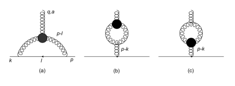
Figure 1: Diagrams that contribute to the mixing between ${\cal O}_{W}$ and ${\cal O}_{4}$. The black dot denotes the insertion of ${\cal O}_{W}$.

It immediately follows that the following linear combination is the eigenstate of the RG evolution

$${\cal O}_{W}+\frac{\gamma_{12}}{\gamma_{W}-\gamma_{4}}{\cal O}_{4}={\cal O}_{W}-\frac{9N_{c}^{2}}{3N_{c}^{2}+4}{\cal O}_{4}.$$ (93)

Since this operator has a rather large anomalous dimension $\gamma_{W}\sim 10$, in particular larger than $\gamma_{4}$ by a factor of about 2, at high enough renormalization scales $\mu^{2}$ one has

$$\langle{\cal O}_{W}\rangle\approx\frac{9N_{c}^{2}}{3N_{c}^{2}+4}\langle{\cal O}_{4}\rangle\approx 2.61\langle{\cal O}_{4}\rangle,$$ (94)

or equivalently,

$$E\approx\frac{9N_{c}^{2}}{4(3N_{c}^{2}+4)}f_{0}\approx 0.65f_{0}.$$ (95)

Comparing with (65), we see that the operator $\tilde{F}D^{2}F$ also contributes to the trace part.

We have thus argued that the matrix element of the Weinberg operator is dominated by its mixing with the total derivative operator ${\cal O}_{4}$ which is further related to the twist-four operator relevant to polarized DIS. Our result urges one to revisit previous estimates of $\langle{\cal O}_{W}\rangle$. For instance, Ref. Bigi:1990kz suggested the following ansatz

$$\langle N|\frac{g^{3}}{16\pi^{2}}f^{abc}F_{\mu\nu}^{a}F^{\mu\alpha}_{b}F_{c\alpha}^{\nu}|N\rangle=\Lambda_{QCD}^{2}\langle N|\frac{\alpha_{s}}{4\pi}F_{\mu\nu}^{a}F^{\mu\nu}_{a}|N\rangle.$$ (96)

While such a relation may give a reasonable order-of-magnitude estimate, it has to be interpreted with great care. Both sides vanish in the forward limit and in the off-forward case the matrix elements are sensitive to the spin polarization. If one tries to relate the coefficients of $\Delta\cdot S$ in the near-forward limit, the right hand side essentially gives $\Delta\Sigma$, the quark helicity contribution to the nucleon spin, while the left hand side is related to the parameter $f_{0}$ which enters the twist-four corrections in polarized DIS as we have shown. There is no known relation between the two quantities.

VI Conclusions

In this paper we have studied the roles of $CP$-odd gluonic operators $\tilde{F}^{\mu\nu}F_{\mu\nu}$ and $\tilde{F}_{\mu\nu}F^{\mu\alpha}F^{\nu}_{\alpha}$ in QCD spin physics. These high-dimension, high-twist operators usually do not appear in the standard description of spin-dependent phenomena in terms of twist-two (and sometimes twist-three) distributions. However, with the future Electron-Ion Collider poised to reveal the gluonic contributions to the nucleon spin and various polarization observables, it is worthwhile and maybe necessary to expand our scope to the twist-four sector. Indeed, we have shown in (27) that the twist-two observables $\Delta\Sigma$ and $\Delta G$ are related to a certain twist-four correlator. Moreover, $\tilde{F}(x)$ directly shows up in a recent calculation of the $g_{1}(x)$ structure function Tarasov:2020cwl . As we have seen, $\tilde{F}(x)$ contains $\Delta G(x)$, and this should be taken into account when fully extracting the implications of the result in Tarasov:2020cwl . Concerning the dimension-six, Weinberg operator $\tilde{F}_{\mu\nu}F^{\mu\alpha}F^{\nu}_{\alpha}$, hopefully our result better motivates a precise determination of the parameter $f_{0}$ through the measurement of the $g_{1}(x)$ structure function. This could be a useful input to the studies of the nucleon electric dipole moment.

References

• (1) Y. Hatta and Y. Zhao, Phys. Rev. D 102, no.3, 034004 (2020) doi:10.1103/PhysRevD.102.034004 [arXiv:2006.02798 [hep-ph]].
• (2) National Academies of Sciences, Engineering, and Medicine. 2018. An Assessment of U.S.-Based Electron-Ion Collider Science. Washington, DC: The National Academies Press. https://doi.org/10.17226/25171.
• (3) R. L. Jaffe and A. Manohar, Nucl. Phys. B 337, 509-546 (1990) doi:10.1016/0550-3213(90)90506-9
• (4) H. Y. Cheng, Int. J. Mod. Phys. A 11, 5109-5182 (1996) doi:10.1142/S0217751X96002364 [arXiv:hep-ph/9607254 [hep-ph]].
• (5) D. Mueller and O. V. Teryaev, Phys. Rev. D 56, 2607-2613 (1997) doi:10.1103/PhysRevD.56.2607 [arXiv:hep-ph/9701413 [hep-ph]].
• (6) A. Tarasov and R. Venugopalan, [arXiv:2008.08104 [hep-ph]].
• (7) C. Y. Seng, Phys. Rev. Lett. 122, no.7, 072001 (2019) doi:10.1103/PhysRevLett.122.072001 [arXiv:1809.00307 [hep-ph]].
• (8) S. Weinberg, Phys. Rev. Lett. 63, 2333 (1989) doi:10.1103/PhysRevLett.63.2333.
• (9) I. I. Balitsky and V. M. Braun, Phys. Lett. B 267, 405-410 (1991) doi:10.1016/0370-2693(91)90954-O
• (10) D. B. Kaplan and A. Manohar, Nucl. Phys. B 310, 527-547 (1988) doi:10.1016/0550-3213(88)90090-9
• (11) D. de Florian and W. Vogelsang, Phys. Rev. D 99, no.5, 054001 (2019) doi:10.1103/PhysRevD.99.054001 [arXiv:1902.04636 [hep-ph]].
• (12) X. D. Ji, Phys. Lett. B 289, 137-142 (1992) doi:10.1016/0370-2693(92)91375-J.
• (13) Y. Hatta, K. Tanaka and S. Yoshida, JHEP 02, 003 (2013) doi:10.1007/JHEP02(2013)003 [arXiv:1211.2918 [hep-ph]].
• (14) Y. Koike, K. Yabe and S. Yoshida, Phys. Rev. D 101, no.5, 054017 (2020) doi:10.1103/PhysRevD.101.054017 [arXiv:1912.11199 [hep-ph]].
• (15) S. L. Adler, Phys. Rev. 177, 2426-2438 (1969) doi:10.1103/PhysRev.177.2426
• (16) J. Kodaira, Nucl. Phys. B 165, 129-140 (1980) doi:10.1016/0550-3213(80)90310-7
• (17) M. Burkardt and Y. Koike, Nucl. Phys. B 632, 311-329 (2002) doi:10.1016/S0550-3213(02)00263-8 [arXiv:hep-ph/0111343 [hep-ph]].
• (18) J. de Vries, E. Mereghetti, C. Y. Seng and A. Walker-Loud, Phys. Lett. B 766, 254-262 (2017) doi:10.1016/j.physletb.2017.01.017 [arXiv:1612.01567 [hep-lat]].
• (19) R. L. Jaffe and X. D. Ji, Nucl. Phys. B 375 (1992), 527-560 doi:10.1016/0550-3213(92)90110-W
• (20) I. I. Balitsky, V. M. Braun, Y. Koike and K. Tanaka, Phys. Rev. Lett. 77 (1996), 3078-3081 doi:10.1103/PhysRevLett.77.3078 [arXiv:hep-ph/9605439 [hep-ph]].
• (21) A. V. Efremov, K. Goeke and P. Schweitzer, Phys. Rev. D 67 (2003), 114014 doi:10.1103/PhysRevD.67.114014 [arXiv:hep-ph/0208124 [hep-ph]].
• (22) E. V. Shuryak and A. I. Vainshtein, Nucl. Phys. B 201, 141 (1982) doi:10.1016/0550-3213(82)90377-7
• (23) I. I. Balitsky, V. M. Braun and A. V. Kolesnichenko, Phys. Lett. B 242, 245-250 (1990) doi:10.1016/0370-2693(90)91465-N [arXiv:hep-ph/9310316 [hep-ph]].
• (24) X. D. Ji and P. Unrau, Phys. Lett. B 333, 228-232 (1994) doi:10.1016/0370-2693(94)91035-9 [arXiv:hep-ph/9308263 [hep-ph]].
• (25) H. Kawamura, T. Uematsu, J. Kodaira and Y. Yasui, Mod. Phys. Lett. A 12, 135-143 (1997) doi:10.1142/S0217732397000133 [arXiv:hep-ph/9603338 [hep-ph]].
• (26) J. A. Gracey, JHEP 04, 127 (2009) doi:10.1088/1126-6708/2009/04/127 [arXiv:0903.4623 [hep-ph]].
• (27) V. M. Braun and A. N. Manashov, JHEP 01, 085 (2012) doi:10.1007/JHEP01(2012)085 [arXiv:1111.6765 [hep-ph]].
• (28) A. Y. Morozov, Sov. J. Nucl. Phys. 40, 505 (1984)
• (29) A. Y. Morozov, ITEP-190-1983.
• (30) E. Braaten, C. S. Li and T. C. Yuan, Phys. Rev. Lett. 64, 1709 (1990) doi:10.1103/PhysRevLett.64.1709.
• (31) E. V. Shuryak and A. I. Vainshtein, Nucl. Phys. B 199, 451-481 (1982) doi:10.1016/0550-3213(82)90355-8
• (32) J. Kodaira, T. Nasuno, H. Tochimura, K. Tanaka and Y. Yasui, Prog. Theor. Phys. 99, 315-320 (1998) doi:10.1143/PTP.99.315 [arXiv:hep-ph/9712395 [hep-ph]].
• (33) I. I. Y. Bigi and N. G. Uraltsev, Nucl. Phys. B 353, 321-336 (1991) doi:10.1016/0550-3213(91)90339-Y