Disentangling enantiosensitivity from dichroism using bichromatic fields

Abstract

We discuss how tensorial observables, available in photoelectron angular distributions resulting from interaction between isotropic chiral samples and cross polarized $\omega$-$2\omega$ bichromatic fields, allow for chiral discrimination without chiral light and within the electric-dipole approximation. We extend the concept of chiral setup [Phys. Rev. A 98, 063428 (2018)], which explains how chiral discrimination can be achieved in the absence of chiral light, to the case of tensorial observables. We derive selection rules for the enantiosensitivity and dichroism of the $b_{l,m}$ coefficients describing the photoelectron angular distribution valid for both weak and strong fields and for arbitrary $\omega$-$2\omega$ relative phase. Explicit expressions for simple perturbative cases are given. We find that, besides the dichroic non-enantiosensitive [J. Chem. Phys. 151 074106 (2019)], and dichroic-and-enantiosensitive $b_{l,m}$ coefficients found recently [Phys. Rev. A 99, 063406 (2019)], there are also enantiosensitive non-dichroic $b_{l,m}$ coefficients. These reveal the molecular enantiomer independently of the relative phase between the two colors and are therefore observable even in the absence of stabilization of the $\omega$-$2\omega$ relative phase.

I Introduction

More than two centuries after the pioneering observations of Biot and Arago (Lowry, 1964), the interaction between light and chiral matter (Berova et al., 2012) remains a very active field of research (Eibenberger et al., 2017; Yachmenev et al., 2019; Goetz et al., 2019a; Ayuso et al., 2019; Cao and Qiu, 2018). This research effort is fueled not only by the interest in finding new ways of manipulating light and matter but also by the homochirality of life. While the molecule-molecule interactions that take place in biological systems are often strongly enantiosensitive (Noyori, 2002), the enantiosensitive response in “traditional” light-matter interactions is usually very weak. This weakness, which limits the potential of light-based applications, is prevalent in situations where the electric-dipole approximation is well justified but the chiral effects appear through small corrections such as the magnetic-dipole interaction (Barron, 2004). Besides ingenious methods to cope with such situations (Rhee et al., 2009; Tang and Cohen, 2011), weakly enantiosensitive responses can be avoided from the outset by relying on chiral effects occurring within the electric-dipole approximation (Ordonez and Smirnova, 2018; Ordonez, 2019).

Among the chiral electric-dipole effects, photoelectron circular dichroism (PECD) (Ritchie, 1976; Böwering et al., 2001; Powis, 2000) is very well established and has been shown to consistently yield strongly enantiosensitive signals across many molecular species (Nahon et al., 2015) and different photoionization regimes (Beaulieu et al., 2016). In PECD, isotropically oriented chiral molecules are photoionized using circularly polarized light and the photoelectron angular distribution displays a so-called forward-backward asymmetry (asymmetry with respect to the polarization plane). This asymmetry is both enantiosensitive (opposite for opposite enantiomers) and dichroic (opposite for opposite polarizations), and results from the lack of mirror symmetry of the chiral molecules (and thus of the light-matter system) with respect to the plane of polarization. For an isotropically oriented achiral molecule and within the electric-dipole approximation (i.e. ignoring light-propagation effects), the light-matter system is mirror-symmetric with respect to the polarization plane and therefore forward-backward asymmetric observables resulting from a single-molecule response are symmetry-forbidden. For a randomly oriented chiral molecule the mirror symmetry of the light-matter system is absent and there are usually no further symmetries preventing the emergence of forward-backward asymmetric observables. In the one-photon case, the forward-backward asymmetry results from the non-zero molecular rotational invariant describing the average circular polarization of the photoionization-dipole vector field (Ordonez and Smirnova, ).

Very recently, the response of chiral molecules to more elaborate field polarizations has been investigated in the multiphoton and strong-field regimes (Demekhin et al., 2018; Demekhin, 2019; Rozen et al., 2019). In these works, a bichromatic field with frequencies $\omega$ and $2\omega$ linearly polarized perpendicular to each other yields a new type of enantiosensitive and dichroic asymmetry in the photoelectron angular distribution. The Lissajous figure of this bichromatic field has an eight-like shape for particular phase relations between the two colors, and therefore “rotates” in opposite directions in the first and second halves of its cycle, with the direction of rotation of the field locked to the sign of its $\omega$ component. For example, the rotation is clockwise when the $\omega$ component is positive and counterclockwise when the $\omega$ component is negative. The observed asymmetry in the photoelectron angular distribution corresponds to a correlation between the so-called forward-backward direction and the up-down direction determined by the $\omega$ field (see Fig. 1 in Ref. (Demekhin et al., 2018)). So far, this asymmetry has been analyzed on the basis of a subcycle PECD-like picture where electrons detected in the upper hemisphere have an e.g. positive forward-backward asymmetry because they were produced by a field rotating e.g. clockwise, while the electrons detected in the lower hemisphere have a negative forward-backward asymmetry because they were produced by a field rotating counterclockwise (Demekhin et al., 2018; Rozen et al., 2019). Extensions of this reasoning to account for non-zero asymmetries for other relative phases between the $\omega$ and $2\omega$ components have been considered in Refs. (Demekhin, 2019) and (Rozen et al., 2019).

Here we approach the description of the photoelectron angular distribution taking explicitly into account its tensorial character, the role of tensorial detectors in forming the chiral setup required to distinguish between opposite enantiomers, and the symmetry of the light-matter system. In Sec. II we discuss general considerations regarding how to distinguish between opposite enantiomers in isotropic samples with and without relying on the chirality of a light field. In Sec. III we discuss how tensorial observables can be used for the construction of chiral setups. In section IV we consider the interaction of an $\omega$-2$\omega$ cross polarized field with isotropic molecular samples and derive selection rules for multipolar observables. Then we consider the perturbative description of photoionization and exploit the method presented in Ref. (Ordonez and Smirnova, ) to obtain explicit formulas for some representative $\tilde{b}_{l,m}$ coefficients of the photoelectron angular distribution displaying different combinations of dichroism and enantiosensitivity. Finally, we list our conclusions in Sec. V. Analogous results but for the case of charge multipoles induced via excitation of bound states is presented in Ref. (Ordonez and Smirnova, 2020).

II Chiral probes

Distinguishing between the left version (L) and the right version (R) of a chiral object invariably requires interaction with another chiral object (say R’). The difference between the interactions L+R’ and R+R’ is the essence of any enantiosensitive phenomenon. Here we are interested in the phenomena where light is used to distinguish between opposite enantiomers of an isotropically oriented chiral molecule. In the simplest case, one lets circularly polarized light of a given handedness interact with a chiral sample and measures a scalar, namely the amount of light that is absorbed. In this situation, known as circular dichroism (CD), the chiral probe is the circularly polarized light and its handedness (a pseudoscalar) is given by its helicity, i.e. the projection of the photon spin (the rotation direction of the light at a given point in space, a pseudovector) on the propagation direction of the light (a vector). Another canonical example is optical activity, where one passes linearly polarized light through a chiral sample and measures the rotation of the polarization plane. In this case one measures an angle (a pseudovector). To measure it one must define a positive and a negative direction in the laboratory frame. Although such definition is just as arbitrary as defining what is left and what is right, it is a fundamental step in the measurement process. Once it has been defined, the handedness of the probe is given by the projection of the positive unit angle pseudovector on the propagation direction of the light. That is, the chiral probe in this case is the chiral setup formed by the (achiral) light and the (achiral) detector (which encodes the definition of positive and negative rotations) together. This shows how a chiral setup may probe the handedness of a molecule in the absence of chiral light (Ordonez, 2019).

Circular dichroism and optical activity have in common that the handedness of the chiral probe relies on the propagation direction of the light. Since that propagation direction is immaterial within the electric-dipole approximation, unless one considers corrections to the electric-dipole approximation the probe ceases to be chiral and both effects vanish. To the extent that such corrections are typically small at the single molecule level, these effects are also correspondingly small. In order to obtain bigger enantiosensitive signals at the single-molecule level, a probe which is chiral within the electric-dipole approximation is required. Furthermore, if the result of the measurement is a scalar (like in circular dichroism), the light itself must be chiral. The concept of light which is chiral within the electric-dipole approximation, i.e. locally-chiral light, has been recently developed in Ref. (Ayuso et al., 2019). If the result of the measurement is a polar vector, such as a photoelectron current, then the detector required to measure the vector must define (again, in an arbitrary fashion) a positive and a negative direction. In addition, if the polarization of the light allows the definition of a pseudovector, as is the case for example for circularly polarized light, where the pseudovector indicates the photon’s spin, then one can define a chiral setup with its handedness given by the projection of the light pseudovector on the positive direction defined by the detector. This type of chiral setup is common to a series of recently discovered phenomena that range from rotational dynamics (Patterson et al., 2013; Patterson and Doyle, 2013; Lehmann, 2018) to photoionization (Ritchie, 1976; Böwering et al., 2001; Powis, 2000; Lux et al., 2012), and it was recently discussed in Ref. (Ordonez and Smirnova, 2018). In what follows we will extend the concept of chiral setups, to include those that rely on tensors of rank 2 (relevant for the results in Refs. (Demekhin et al., 2018; Demekhin, 2019; Rozen et al., 2019)) and higher.

III Tensor observables and chiral setups

Figure 1: Chiral setups consisting of a Lissajous figure and detectors. Counts on red/blue detectors are added/subtracted. The color of the Lissajous figure indicates the phase of the oscillation. (a) A field circularly polarized in the $xy$ plane and a detector for $\tilde{b}_{1,0}$. (b) and (c) A cross-polarized $\omega$-2$\omega$ field in the $xz$ plane and a detector for $\tilde{b}_{2,-2}$ and $\tilde{b}_{3,-2}$ respectively.

Second and higher-rank tensors emerge naturally for observables which depend on a vector. Charge densities and photoelectron angular distributions (PADs) offer exactly such kind of observable and, as any other function which depends on a vector, they can be expanded as

$$W(\vec{k})=\sum_{l,m}\tilde{b}_{l,m}\left(k\right)\tilde{Y}_{l}^{m}(\hat{k}),$$ (1)

where $\vec{k}$ is the photoelectron momentum and we have chosen to do the expansion in terms of real spherical harmonics $\tilde{Y}_{l}^{m}$. In the case of a charge distribution we replace the photoelectron momentum $\vec{k}$ by the position $\vec{r}$ and $\tilde{b}_{l,m}$ could be a time dependent quantity (see (Ordonez and Smirnova, 2020)). The $\tilde{b}_{l,m}$ coefficients not only encode all the information contained in $W(\vec{k})$ but are also examples of tensors of rank $l$ (see e.g. Sec. 4.10 in Ref. (Brink and Satchler, 1968)).

In principle, the measurement of a particular $\tilde{b}_{l,m}$ coefficient can be performed directly by using a detector with a structure that reflects the corresponding $\tilde{Y}_{l}^{m}$. For example, a detector for $\tilde{b}_{0,0}$ would simply sum the counts in all directions. A detector for $\tilde{b}_{1,0}$ would have two plates arranged as in Fig. 1a, so that it would add all the counts on one of them (red) and subtract all the counts on the other (blue). The choice of which plate adds and which plate subtracts is what physically defines the $\hat{z}$ direction of the laboratory frame. A detector for $\tilde{b}_{2,-2}$ would have four plates arranged as in Fig. 1b, with a pair of opposite plates adding counts and the other pair subtracting counts. In this case, the detector defines the directions that correspond to a positive correlation between $x$ and $y$, and those that correspond to a negative correlation between $x$ and $y$. Analogously, a detector for $\tilde{b}_{3,-2}$ has eight plates arranged as in Fig. 1c, and distinguishes positive from negative correlations of $x$, $y$, and $z$.

If we now take into account the electric field, then the combination of a $\tilde{b}_{l,m}$-specific detector and the Lissajous figure of the electric field can make up a chiral setup as shown in Fig. 1. These setups are non-superimposable on their mirror images. This is particularly simple to see in Fig. 1 for reflections with respect to the polarization plane, which do not change the Lissajous figure but do swap blue and red plates.

Of course, a chiral setup is only relevant if the light-matter system is indeed asymmetric enough that it can yield a corresponding non-zero $\tilde{b}_{l,m}$. In other words, the concept of a chiral setup answers the question of how we can distinguish opposite enantiomers without relying on the chirality of light, but it is the lack of symmetry of the light-matter system itself the deciding factor which determines the emergence of an enantiosensitive observable in the first place (see e.g. Fig. 2 in Ref. (Ordonez and Smirnova, 2018)). We now turn to the analysis of a specific family of Lissajous figures to illustrate this in detail.

IV $\boldsymbol{\omega}$-2$\boldsymbol{\omega}$ cross polarized field

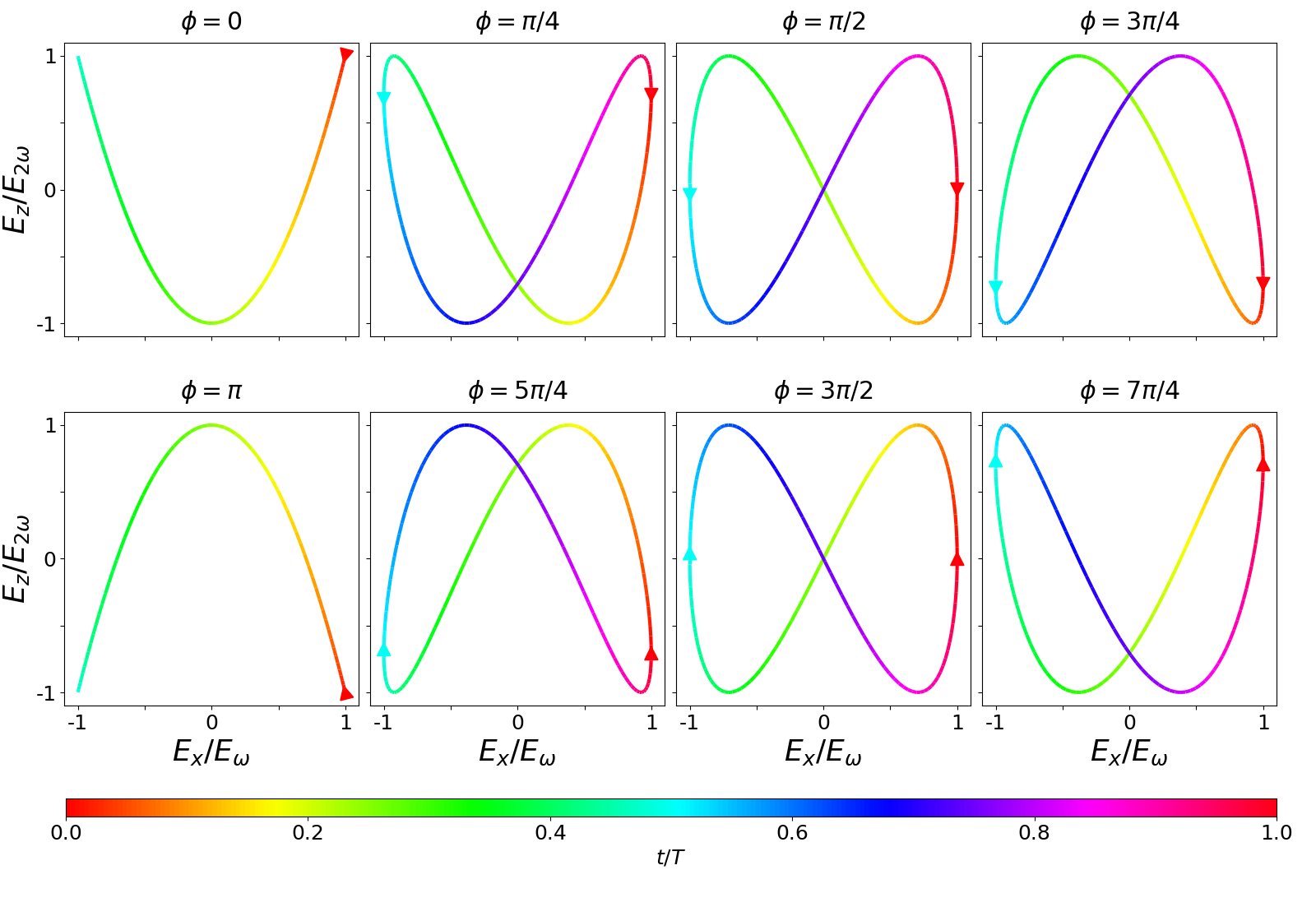
Figure 2: Lissajous curves of the field (2) for different values of $\phi$. The position of the red arrow indicates $t=0$.

Consider a two-color field of the form

$$\vec{E}\left(t\right)=E_{\omega}\cos\left(\omega t\right)\hat{x}+E_{2\omega}\cos\left(2\omega t+\phi\right)\hat{z}$$ (2)

This field is illustrated in Fig. 2 for different phases $\phi$. If we denote rotations by $\pi$ around the $z$ axis by $\hat{R}_{z}^{\pi}$ and time shifts of $\pi/\omega$ by $T_{\pi/\omega}$, then the joint system (field and isotropic chiral molecules) is invariant with respect to $\hat{R}_{z}^{\pi}\hat{T}_{\pi/\omega}$. Clearly, the resulting observables must also be invariant with respect to $\hat{R}_{z}^{\pi}\hat{T}_{\pi/\omega}$. That is, the symmetry-allowed $\tilde{b}_{l,m}$ coefficients must satisfy $\hat{R}_{z}^{\pi}\hat{T}_{\pi/\omega}\tilde{b}_{l,m}\tilde{Y}_{l}^{m}=\tilde{b}_{l,m}\tilde{Y}_{l}^{m}$. This corresponds to two scenarios: either $\hat{R}_{z}^{\pi}\tilde{Y}_{l}^{m}=\tilde{Y}_{l}^{m}$ and $\tilde{b}_{l,m}$ contains only frequencies $2n\omega$, or $\hat{R}_{z}^{\pi}\tilde{Y}_{l}^{m}=-\tilde{Y}_{l}^{m}$ and $\tilde{b}_{l,m}$ contains only frequencies $\left(2n+1\right)\omega$, where $n=0,1,2,\dots$ Furthermore, since the a reflection $\hat{\sigma}_{y}$ with respect to the $y=0$ plane swaps the enantiomers while leaving the field invariant, an enantiosensitive $\tilde{b}_{l,m}$ is associated to a $\tilde{Y}_{l}^{m}$ satisfying $\hat{\sigma}_{y}\tilde{Y}_{l}^{m}=-\tilde{Y}_{l}^{m}$. And, since a rotation $\hat{R}_{x}^{\pi}$ of $\pi$ around the $x$ axis changes the phase $\phi$ in the field by $\pi$ while leaving the molecules invariant, a dichroic $\tilde{b}_{l,m}$ is associated to a $\tilde{Y}_{l}^{m}$ satisfying $\hat{R}_{x}^{\pi}\tilde{Y}_{l}^{m}=-\tilde{Y}_{l}^{m}$. These properties, which are valid independently of the ionization regime, are summarized in Tabs. 1 and 2.

Evidently, the values of $l$ and $m$ that determine whether a given $\tilde{b}_{l,m}$ is symmetry-allowed and whether it is enantiosensitive and/or dichroic depends on how the field is oriented with respect to the axes. The choice made here [Eq. (2)] yields the rather simple conditions in Tabs. 1 and 2. Conditions corresponding to other choices are given in Appendix A.1 for the sake of comparison with Refs. (Demekhin et al., 2018; Demekhin, 2019; Rozen et al., 2019).

Tables 1 and 2 reveal two important features. First, the spatial structure of the response depends on whether it oscillates with a frequency which is an even (including zero) or an odd multiple of the fundamental frequency (see also (Neufeld et al., 2019)). Second, in contrast to a circularly polarized field where dichroism goes hand in hand with enantiosensitivity, the symmetry of the field (2) leads to four types of signals:

1. Non-dichroic non-enantiosensitive.

2. Dichroic and enantiosensitive.

3. Dichroic non-enantiosensitive.

4. Enantiosensitive non-dichroic.

Type (i) and type (ii) signals are well known from traditional CD and PECD. Type (iii) signals are well known in atoms subject to light fields whose Lissajous figure is not symmetric under spatial inversion (Yin et al., 1992). They have also been recently calculated for the case of randomly oriented chiral molecules (Goetz et al., 2019b) for parallel polarizations of $\omega$ and $2\omega$. Here, type (iii) signals are due to the asymmetry of the field (2) along the $z$ direction (see Fig. 2). Type (iv) signals are more exotic but apparently they can also occur in the context of magnetic effects beyond the electric-dipole approximation (Wagnière, 1989; Wagnière and Rikken, 2011), where as far as the authors know they remain to be confirmed by experiment. As we will show next, photoionization may prove to be a better candidate for experimentally measuring type (iv) signals.

$\tilde{b}_{l,m}$	$\left(l,m\right)$ condition
Symmetry-allowed at $2n\omega$	even $m$
Symmetry-allowed at $\left(2n+1\right)\omega$	odd $m$
Enantiosensitive	$m<0$
Dichroic	[(odd $l-m$) and ($m\geq 0$)] or
	(even $l-m$) and ($m<0$)

Table 1: Conditions imposed by symmetry on the $\tilde{b}_{l,m}$ coefficients for a field (2) interacting with an isotropic sample of molecules.

Symmetry-allowed $\tilde{b}_{l,m}$	$\left(l,m\right)$ condition at $2n\omega$	$\left(l,m\right)$ condition at $\left(2n+1\right)\omega$
Enantiosensitive and dichroic	(even $l$) and (even $m<0$)	(odd $l$) and (odd $m<0$)
Enantiosensitive non-dichroic	(odd $l$) and (even $m<0$)	(even $l$) and (odd $m<0$)
Dichroic non-enantiosensitive	(odd $l$) and (even $m>0$)	(even $l$) and (odd $m>0$)

Table 2: $\left(l,m\right)$ conditions derived from Tab. 1 for non-vanishing enantiosensitive and/or dichroic $\tilde{b}_{l,m}$ coefficients.

Photoionization

The photoelectron angular distribution accumulated over many cycles of the field (2) corresponds to a signal with zero frequency and must satisfy the conditions given in Tab. 1 for frequencies $2n\omega$. For convenience, we list the properties of the symmetry-allowed $\tilde{b}_{l,m}$ coefficients for $l$ up to four in Tab. 3. From this table we can see that e.g. $\tilde{b}_{1,0}$ is dichroic but not enantiosensitive, $\tilde{b}_{2,-2}$ is enantiosensitive and dichroic, and $\tilde{b}_{3,-2}$ is enantiosensitive but not dichroic. Since $\tilde{Y}_{1}^{0}(\hat{k})\propto k_{z}$, $\tilde{Y}_{2}^{-2}(\hat{k})\propto k_{x}k_{y}$, and $\tilde{Y}_{3}^{-2}(\hat{k})\propto k_{x}k_{y}k_{z}$, then $\tilde{b}_{1,0}$ is associated to asymmetry along the direction of the $2\omega$ field ($\hat{z}$), $\tilde{b}_{2,-2}$ is associated to correlations between the direction of the $\omega$ field ($\hat{x}$) and the direction perpendicular to the polarization plane ($\hat{y}$), and $\tilde{b}_{3,-2}$ is associated to correlations of the three directions corresponding to the $\omega$ field ($\hat{x}$), the $2\omega$ field $(\hat{z})$, and the perpendicular to the polarization plane ($\hat{y}$).

In Ref. (Ordonez and Smirnova, ) we showed that, in general, a $\tilde{b}_{l,m}$ coefficient is enantiosensitive if and only if it results from interference between pathways with $N_{1}$ and $N_{2}$ photons, respectively, and $l+N_{1}+N_{2}$ is odd; or if it results from a direct pathway and $l$ is odd. These conditions together with Tab. (2) tell us that a dichroic non-enantiosensitive $\tilde{b}_{l,m}$ (with odd $l$) can only occur as the result of interference between pathways involving an even and an odd number of photons, respectively (so that $N_{1}+N_{2}$ is odd and $l+N_{1}+N_{2}$ is even). For example, $\tilde{b}_{1,0}$ contributes to the photoelectron peak where absorption of two $\omega$ photons interferes with absorption of one $2\omega$ photon (see Fig. 3a). The same condition (odd $N_{1}+N_{2}$) applies for a dichroic and enantiosensitive $\tilde{b}_{l,m}$ (even $l$) such as $\tilde{b}_{2,-2}$. In contrast, an enantiosensitive non-dichroic $\tilde{b}_{l,m}$ (odd $l$) can occur as the result of either a direct pathway involving at least one $\omega$ photon and one $2\omega$ photon, or as the result of interference between two pathways both with an even or both with an odd number of photons (even $N_{1}+N_{2}$). For example, $\tilde{b}_{3,-2}$ contributes to the photoelectron peak corresponding to absorption of one $\omega$ photon followed by absorption of one $2\omega$ photon (see Fig. 3b) and vice versa, or as the result of interference between absorption of two $2\omega$ photons and four $\omega$ photons.

Symmetry-allowed	$\tilde{b}_{0,0}$	$\tilde{b}_{1,0}$	$\tilde{b}_{2,-2}$	$\tilde{b}_{2,0}$	$\tilde{b}_{2,2}$	$\tilde{b}_{3,-2}$	$\tilde{b}_{3,0}$	$\tilde{b}_{3,2}$	$\tilde{b}_{4,-4}$	$\tilde{b}_{4,-2}$	$\tilde{b}_{4,0}$	$\tilde{b}_{4,2}$	$\tilde{b}_{4,4}$
Enantiosensitive	N	N	Y	N	N	Y	N	N	Y	Y	N	N	N
Dichroic	N	Y	Y	N	N	N	Y	Y	Y	Y	N	N	N

Table 3: Dichroism and enantiosensitivity of symmetry-allowed $\tilde{b}_{l,m}$ coefficients describing the photoelectron angular distribution (1) resulting from interaction with the field (2) for $l$ up to 4. N=No and Y=Yes.

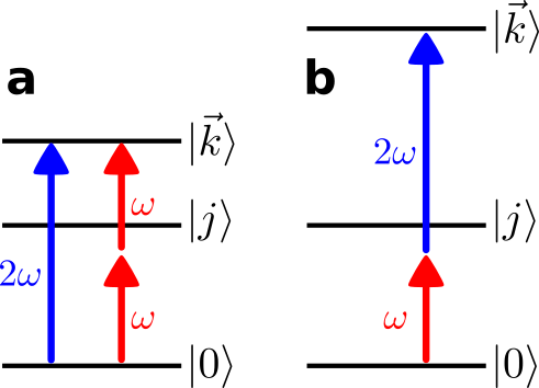
Figure 3: a. Simplest scheme to generate a non-zero $\tilde{b}_{1,0}$ (dichroic non-enantiosensitive) and $\tilde{b}_{2,-2}$ (dichroic and enantiosensitive) using the field (2). b. Simplest scheme to generate a non-zero $\tilde{b}_{3,-2}$ (enantiosensitive non-dichroic). $|0\rangle$ and $|j\rangle$ are bound states and $|\vec{k}\rangle$ is a continuum state.

As an example, let us calculate explicit expressions for $\tilde{b}_{1,0}$, $\tilde{b}_{2,-2}$, and $\tilde{b}_{3,-2}$. For the process depicted in Fig. 3a , the interference between the two pathways gives rise to a non-zero orientation-averaged $\tilde{b}_{1,0}$ given by (Ordonez and Smirnova, ) (see Appendix)

$$\tilde{b}_{1,0}\left(k\right)=A^{\left(1\right)*}A^{\left(2\right)}g_{1,0}f_{1,0}+\mathrm{c.c.},$$ (3)

where $A^{\left(1\right)}$ and $A^{\left(2\right)}$ are complex-valued constants depending on detunings and pulse envelopes, c.c. denotes the complex conjugate, $g_{1,0}$ is a (complex-valued) molecular rotational invariant, and $f_{1,0}$ is a setup (i.e. field + detector) rotational invariant. $g_{1,0}$ is a scalar (in contrast to a pseudoscalar) and therefore $\tilde{b}_{1,0}$ is not enantiosensitive. The expression for $f_{1,0}$ reads as

$$f_{1,0}\equiv\left(\hat{z}\cdot\vec{E}_{2\omega}^{*}\right)\left(\vec{E}_{\omega}\cdot\vec{E}_{\omega}\right)=E_{2\omega}E_{\omega}^{2}e^{i\phi},$$ (4)

where $\vec{E}_{2\omega}\equiv E_{2\omega}e^{-i\phi}\hat{y}$, $\vec{E}_{\omega}\equiv E_{\omega}\hat{z}$. Equation (4) shows that the setup rotational invariant $f_{1,-1}$ is a scalar involving the field vectors $\vec{E}_{2\omega}$ and $\vec{E}_{\omega}$, and the axis $\hat{z}$. As discussed in Sec. III, the axis vector $\hat{z}$ is defined by the detector needed to measure $\tilde{b}_{1,0}$. From Eq. (4) it is evident that $f_{1,0}$ changes sign when $\phi$ is shifted by $\pi$, and therefore $\tilde{b}_{1,0}$ is dichroic.

Similarly, the interference between the two pathways in Fig. 3a also gives rise to a non-zero orientation-averaged $\tilde{b}_{2,-2}$ given by (see Appendix A.2)

$$\tilde{b}_{2,-2}=A^{\left(1\right)*}A^{\left(2\right)}g_{2,-2}f_{2,-2}+\mathrm{c.c.},$$ (5)

where the molecular rotational invariant $g_{2,-2}$ is a (complex-valued) pseudoscalar³ and therefore $\tilde{b}_{2,-2}$ is enantiosensitive. The setup rotational invariant, given by

$$f_{2,-2}\equiv\left[\hat{x}\cdot\left(\hat{y}\times\vec{E}_{2\omega}^{*}\right)\right]\left(\vec{E}_{\omega}\cdot\vec{E}_{\omega}\right)=E_{2\omega}E_{\omega}^{2}e^{i\phi},$$ (6)

is also a pseudoscalar and it involves the $\hat{x}$ and $\hat{y}$ axes, which are defined by the detector needed to measure $\tilde{b}_{2,-2}$ (see Sec. III). Just like $g_{2,-2}$ is a pseudoscalar that distinguishes between molecules with opposite handedness, $f_{2,1}$ is a pseudoscalar that distinguishes between chiral setups of opposite handedness. Note that the detector for $\tilde{b}_{2,-2}$ does not directly tell apart a positive $x$ from a negative $x$, or a positive $y$ from a negative $y$. It only tells apart positive correlations of $x$ and $y$ from negative correlations of $x$ and $y$. This is consistent with the invariance of $f_{2,-2}$ with respect to a simultaneous inversion of $\hat{x}$ and $\hat{y}$. Furthermore, Eq. (6) shows that $f_{2,-2}$ changes sign when $\phi$ is shifted by $\pi$, and therefore $\tilde{b}_{2,-2}$ is dichroic. We remark, that although the right hand side of $f_{1,0}$ and $f_{2,-2}$ looks exactly the same after performing the vector operations, they emerge from different setup rotational invariants of a different physical nature: one is a scalar involving only the $\hat{z}$ axis, and the other is a pseudoscalar involving correlation between the $\hat{x}$ and $\hat{y}$ axes.

We consider now the simplest process leading to the enantiosensitive but not dichroic term $\tilde{b}_{3,-2}$, i.e. we consider the absorption of one $\omega$ photon and one $2\omega$ photon, resonantly enhanced through a bound state as shown in Fig. 3b. In this case we get (see Appendix A.2)

$$\tilde{b}_{3,-2}\left(k\right) =\left|A^{\left(2\right)}\right|^{2}g_{3,-2}f_{3,-2},$$ (7)

where the rotational invariant $g_{3,-2}$ is a (complex-valued) pseudoscalar³ which makes $\tilde{b}_{3,-2}$ enantiosensitive and the setup rotational invariant $f_{3,-2}$ is given by

$$f_{3,-2}\equiv\left[\hat{y}^{\mathrm{L}}\cdot\left(\hat{z}^{\mathrm{L}}\times\hat{x}^{\mathrm{L}}\right)\right]\left(\vec{E}_{2\omega}^{\mathrm{L}*}\cdot\vec{E}_{2\omega}^{\mathrm{L}}\right)\left(\vec{E}_{\omega}^{\mathrm{L}*}\cdot\vec{E}_{\omega}^{\mathrm{L}}\right)=-E_{\omega}^{2}E_{2\omega}^{2}.$$ (8)

$f_{3,-2}$ is also a pseudoscalar, however it does not record $\phi$ and $\tilde{b}_{3,-2}$ is therefore not dichroic. The robustness of $f_{3,-2}$ against changes of $\phi$ means that, recording $\tilde{b}_{3,-2}$ allows distinguishing opposite enantiomers in the absence of stabilization of the $\omega$-2$\omega$ phase shift $\phi$.

Equations (3)-(8) confirm our expectations based on general symmetry arguments according to which $\tilde{b}_{1,0}$ is dichroic non-enantiosensitive, $\tilde{b}_{2,-2}$ is dichroic and enantiosensitive, and $\tilde{b}_{3,-2}$ is enantiosensitive non-dichroic. In addition, these equations show that $\tilde{b}_{1,0}$, $\tilde{b}_{2,-2}$, and $\tilde{b}_{3,-2}$ are in general not zero for the specific processes considered here. This is important because although a given $\tilde{b}_{l,m}$ may be symmetry allowed according to the general symmetry analysis above, further “hidden” symmetries involved in a specific process may forbid it. For example, although the geometry of a monochromatic elliptical field allows for a non-zero $\tilde{b}_{3,-2}$, a “hidden” symmetry related to the photon ordering ensures it vanishes (see Appendix A.2). However, it must be kept in mind that the hidden symmetry preventing a non-zero $\tilde{b}_{3,-2}$ for elliptical fields is specific to the 2-photon process we investigated here, so it may be broken in higher order processes or in the strong field regime. That is, photoionization induced by elliptically polarized strong fields may indeed yield a non-zero enantiosensitive non-dichroic $\tilde{b}_{3,-2}$ coefficient. This would be analogous to how $\tilde{b}_{2,-2}$ is symmetry-forbidden in the elliptical one-photon case (see (Ordonez and Smirnova, )) but it is symmetry allowed in the elliptical strong-field case (Bashkansky et al., 1988).

V Conclusions

We discussed how tensorial observables offer new opportunities for constructing chiral setups able to distinguish between opposite enantiomers in isotropic samples without relying on the chirality of light. As a concrete example we considered the interaction of an $\omega$-2$\omega$ cross polarized field with isotropic samples and we found selection rules for $l$ and $m$ that specify if a multipole coefficient $\tilde{b}_{l,m}$ is symmetry allowed, if it is dichroic (sensitive to changes of $\pi$ in the $\omega$-$2\omega$ relative phase), and if it is enantiosensitive. These $\tilde{b}_{l,m}$ coefficients are relevant in the description of photoelectron angular distributions and in the description of induced multipoles of bound charge distributions (discussed elsewhere). We found that the enantiosensitivity and the dichroism of a $\tilde{b}_{l,m}$ coefficient are in general independent of each other. That is, in addition to the usual types of $\tilde{b}_{l,m}$ coefficients in isotropic samples, namely: (i) non-dichroic non-enantiosensitive and (ii) dichroic and enantiosensitive and (iii) dichroic non-enantiosensitive, we found the more exotic possibility of (iv) enantiosensitive non-dichroic $\tilde{b}_{l,m}$ coefficients.

We derived analytic expressions for the lowest rank $\tilde{b}_{l,m}$ coefficients in photoelectron angular distributions corresponding to types (ii)-(iv) for the case of one- vs. two-photon absorption and for the case of $\omega+2\omega$ absorption. Unlike type (ii) coefficients, type (iv) coefficients allow enantiomeric discrimination in the absence of stabilization of the $\omega$-$2\omega$ relative phase and remain to be numerically calculated and experimentally observed.

Finally, it is also possible to obtain the type (iv) coefficient $\tilde{b}_{3,-2}$ using monochromatic light with elliptical polarization. However, hidden symmetry prevents this coefficient in the simplest scenario of a two-photon process. The possibility of this hidden symmetry to be violated for higher-order or strong-field processes, or in a more refined description of photoionization remains to be investigated.

Appendix A

A.1 Selection rules for an alternative orientation of the field

In Sec. IV we chose the orientation of the field so as to simplify as much as possible the selection rules for the $\tilde{b}_{l,m}$ coefficients. Here, for the sake of comparison, we consider the alternative orientation used in Refs. (Demekhin et al., 2018; Demekhin, 2019; Rozen et al., 2019), namely

$$\vec{E}\left(t\right)=E_{\omega}\cos\left(\omega t\right)\hat{y}+E_{2\omega}\cos\left(2\omega t+\phi\right)\hat{x}.$$ (A.1)

Tables A.1-A.3 show the analogues of Tabs. 1-3 for the orientation in Eq. A.1. In this case, we see that e.g. $\tilde{b}_{1,1}$, $\tilde{b}_{2,-1}$, and $\tilde{b}_{3,-2}$ are dichroic non-enantiosensitive, enantiosensitive and dichroic, and enantiosensitive non-dichroic, respectively. These are just the correspondingly rotated versions of the coefficients in Sec. (IV). Note that $\tilde{b}_{2,-1}\propto\mathrm{Im}\left\{b_{2,1}\right\}$ is indeed the coefficient discussed in Ref. (Demekhin, 2019).

$\tilde{b}_{l,m}$	$\left(l,m\right)$ condition
non-zero $2n\omega$	(even $l-m$ and $m\geq 0$) or (odd $l-m$ and $m<0$)
non-zero $\left(2n+1\right)\omega$	(odd $l-m$ and $m\geq 0$) or (even $l-m$ and $m<0$)
enantiosensitive	odd $l-m$
dichroic	[(odd $l$) and ($m\geq 0$)] or [(even $l$) and $m<0$]

Table A.1: Same as Tab. 1 for the orientation (A.1).

$\tilde{b}_{l,m}$	$\left(l,m\right)$ condition at $2n\omega$	$(l,m)$ condition at $\left(2n+1\right)\omega$
Enantiosensitive and dichroic	(even $l$) and (odd $m<0$)	(odd $l$) and (even $m\geq 0$)
Enantiosensitive non-dichroic	(odd $l$) and (even $m<0$)	(even $l$) and (odd $m\geq 0$)
Dichroic non-enantiosensitive	(odd $l$) and (odd $m\geq 0$)	(even $l$) and (even $m<0$)

Table A.2: Same as Tab. 2 for the orientation (A.1).

Symmetry-allowed	$\tilde{b}_{0,0}$	$\tilde{b}_{1,1}$	$\tilde{b}_{2,-1}$	$\tilde{b}_{2,0}$	$\tilde{b}_{2,2}$	$\tilde{b}_{3,-2}$	$\tilde{b}_{3,1}$	$\tilde{b}_{3,3}$	$\tilde{b}_{4,-3}$	$\tilde{b}_{4,-1}$	$\tilde{b}_{4,0}$	$\tilde{b}_{4,2}$	$\tilde{b}_{4,4}$
Enantiosensitive	N	N	Y	N	N	Y	N	N	Y	Y	N	N	N
Dichroic	N	Y	Y	N	N	N	Y	Y	Y	Y	N	N	N

Table A.3: Same as Tab. 3 for the orientation (A.1).

A.2 Derivation of the $\boldsymbol{\tilde{b}_{l,m}}$ coefficients in Sec. IV

Derivation of $\boldsymbol{\tilde{b}_{1,0}}$ in Eq. (3)

The process depicted in Fig. 3a yields a $\tilde{b}_{1,0}$ coefficient given by (see Ref. (Ordonez and Smirnova, ))

$$\tilde{b}_{1,0} = \int\mathrm{d}\Omega_{k}^{\mathrm{M}}\int\mathrm{d}\varrho\tilde{Y}_{1}^{0}(\hat{k}^{\mathrm{L}})W^{\mathrm{M}}(\vec{k}^{\mathrm{M}},\varrho)$$ (A.2)

$$= \sqrt{\frac{3}{4\pi}}A^{\left(1\right)*}A^{\left(2\right)}\int\mathrm{d}\Omega_{k}^{\mathrm{M}}\int\mathrm{d}\varrho\left(\hat{k}^{\mathrm{L}}\cdot\hat{z}^{\mathrm{L}}\right)$$

$$\times\left(\vec{d}_{\vec{k}^{\mathrm{M}},0}^{\mathrm{L}}\cdot\vec{E}_{2\omega}^{\mathrm{L}}\right)^{*}\left(\vec{d}_{\vec{k}^{\mathrm{M}},j}^{\mathrm{L}}\cdot\vec{E}_{\omega}^{\mathrm{L}}\right)\left(\vec{d}_{j,0}^{\mathrm{L}}\cdot\vec{E}_{\omega}^{\mathrm{L}}\right)+\mathrm{c.c.},$$

where c.c. denotes the complex conjugate, $\mathrm{L}$ and $\mathrm{M}$ indicate vectors and functions in the laboratory (L) and molecular (M) frames, $\vec{k}$ is the photoelectron momentum, $\hat{k}\equiv\vec{k}/k$, $\varrho\equiv\alpha\beta\gamma$ is the molecular orientation specified by the Euler angles $\alpha\beta\gamma$, $\int\mathrm{d}\varrho\equiv\int_{0}^{2\pi}\mathrm{d}\alpha\int_{0}^{\pi}\mathrm{d}\beta\int_{0}^{2\pi}\mathrm{d}\gamma\sin\beta/8\pi^{2}$ is the normalized integral over all molecular orientations, $\int\mathrm{d}\Omega_{k}^{\mathrm{M}}$ is the integral over all photoelectron directions $\hat{k}^{\mathrm{M}}$, $W^{\mathrm{M}}(\vec{k}^{\mathrm{M}},\varrho)\equiv|a_{\vec{k}^{\mathrm{M}}}\left(\varrho\right)|^{2}$ is the photoelectron angular distribution in the molecular frame for a particular orientation $\varrho$. $a_{\vec{k}^{\mathrm{M}}}\left(\varrho\right)=A^{\left(1\right)}(\vec{d}_{\vec{k}^{\mathrm{M}},0}^{\mathrm{L}}\cdot\vec{E}_{2\omega}^{\mathrm{L}})+A^{\left(2\right)}(\vec{d}_{\vec{k}^{\mathrm{M}},j}^{\mathrm{L}}\cdot\vec{E}_{\omega}^{\mathrm{L}})(\vec{d}_{j,0}^{\mathrm{L}}\cdot\vec{E}_{\omega}^{\mathrm{L}})$ is the probability amplitude of the state $|\vec{k}^{\mathrm{M}}\rangle$, $A^{\left(1\right)}$ and $A^{\left(2\right)}$ are complex-valued constants depending on detunings and pulse envelopes, $\vec{d}_{i,j}\equiv\langle i|\vec{d}|j\rangle$ is the dipole transition matrix element between states $|i\rangle$ and $|j\rangle$, $|\vec{k}\rangle$ is the scattering state describing an outgoing plane wave with photoelectron momentum $\vec{k}$, and $\vec{E}_{\omega}=E_{\omega}\hat{x}$ and $\vec{E}_{2\omega}=E_{2\omega}e^{-i\phi}\hat{z}$ are the Fourier amplitudes of the field (2) at frequencies $\omega$ and $2\omega$. The vectors $\hat{k}^{\mathrm{L}}$, $\vec{d}_{i,j}^{\mathrm{L}}$, $\vec{d}_{\vec{k}^{\mathrm{M}},j}^{\mathrm{L}}$, and $\vec{d}_{j,0}^{\mathrm{L}}$ depend on the molecular orientation $\varrho$ according to $\vec{v}^{\mathrm{L}}=S\left(\varrho\right)\vec{v}^{\mathrm{M}}$, where $S\left(\varrho\right)$ is the rotation matrix taking vectors from the molecular frame to the laboratory frame. Note that only the interference between the two pathways in Fig 3 contributes to $\tilde{b}_{1,0}$ (see Sec. IV).

The integral over orientations yields (see Refs. (Ordonez and Smirnova, ) and (Andrews and Thirunamachandran, 1977))

$$\int\mathrm{d}\varrho\left(\hat{k}^{\mathrm{L}}\cdot\hat{z}^{\mathrm{L}}\right)\left(\vec{d}_{\vec{k}^{\mathrm{M}},0}^{\mathrm{L}}\cdot\vec{E}_{2\omega}^{\mathrm{L}}\right)^{*}\left(\vec{d}_{\vec{k},j}^{\mathrm{L}}\cdot\vec{E}_{\omega}^{\mathrm{L}}\right)\left(\vec{d}_{j,0}^{\mathrm{L}}\cdot\vec{E}_{\omega}^{\mathrm{L}}\right)=\vec{g}^{\left(4\right)}\cdot M^{\left(4\right)}\vec{f}^{\left(4\right)},$$ (A.3)

where $\vec{g}^{\left(4\right)}$ and $\vec{f}^{\left(4\right)}$ are vectors of molecular and setup rotational invariants, respectively,

$$\vec{g}^{\left(4\right)}=\left[\begin{array}[]{c}\left(\hat{k}^{\mathrm{M}}\cdot\vec{d}_{\vec{k}^{\mathrm{M}},0}^{\mathrm{M}*}\right)\left(\vec{d}_{\vec{k}^{\mathrm{M}},j}^{\mathrm{M}}\cdot\vec{d}_{j,0}^{\mathrm{M}}\right)\\ \left(\hat{k}^{\mathrm{M}}\cdot\vec{d}_{\vec{k}^{\mathrm{M}},j}^{\mathrm{M}}\right)\left(\vec{d}_{\vec{k}^{\mathrm{M}},0}^{\mathrm{M}*}\cdot\vec{d}_{j,0}^{\mathrm{M}}\right)\\ \left(\hat{k}^{\mathrm{M}}\cdot\vec{d}_{j,0}^{\mathrm{M}}\right)\left(\vec{d}_{\vec{k}^{\mathrm{M}},0}^{\mathrm{M}*}\cdot\vec{d}_{\vec{k}^{\mathrm{M}},j}^{\mathrm{M}}\right)\end{array}\right],$$ (A.4)

$$M^{\left(4\right)}=\left[\begin{array}[]{ccc}4&-1&-1\\ -1&4&-1\\ -1&-1&4\end{array}\right],$$ (A.5)

$$\vec{f}^{\left(4\right)}=\left[\begin{array}[]{c}\left(\hat{z}^{\mathrm{L}}\cdot\vec{E}_{2\omega}^{\mathrm{L}*}\right)\left(\vec{E}_{\omega}^{\mathrm{L}}\cdot\vec{E}_{\omega}^{\mathrm{L}}\right)\\ \left(\hat{z}^{\mathrm{L}}\cdot\vec{E}_{\omega}^{\mathrm{L}}\right)\left(\vec{E}_{2\omega}^{\mathrm{L}*}\cdot\vec{E}_{\omega}^{\mathrm{L}}\right)\\ \left(\hat{z}^{\mathrm{L}}\cdot\vec{E}_{\omega}^{\mathrm{L}}\right)\left(\vec{E}_{2\omega}^{\mathrm{L}*}\cdot\vec{E}_{\omega}^{\mathrm{L}}\right)\end{array}\right]=\left[\begin{array}[]{c}\left(\hat{z}^{\mathrm{L}}\cdot\vec{E}_{2\omega}^{\mathrm{L}*}\right)\left(\vec{E}_{\omega}^{\mathrm{L}}\cdot\vec{E}_{\omega}^{\mathrm{L}}\right)\\ 0\\ 0\end{array}\right].$$ (A.6)

Replacing Eqs. (A.3)-(A.6) in Eq. (A.3) we obtain

$$\tilde{b}_{1,0}=A^{\left(1\right)*}A^{\left(2\right)}g_{1,0}f_{1,0}+\mathrm{c.c.}$$ (A.7)

where the rotational invariants are given by

$$g_{1,0} \equiv\frac{1}{30}\sqrt{\frac{3}{4\pi}}\int\mathrm{d}\Omega_{k}^{\mathrm{M}}\bigg{[}4\left(\hat{k}^{\mathrm{M}}\cdot\vec{d}_{\vec{k}^{\mathrm{M}},0}^{\mathrm{M}*}\right)\left(\vec{d}_{\vec{k}^{\mathrm{M}},j}^{\mathrm{M}}\cdot\vec{d}_{j,0}^{\mathrm{M}}\right)$$

$$-\left(\hat{k}^{\mathrm{M}}\cdot\vec{d}_{\vec{k}^{\mathrm{M}},j}^{\mathrm{M}}\right)\left(\vec{d}_{\vec{k}^{\mathrm{M}},0}^{\mathrm{M}*}\cdot\vec{d}_{j,0}^{\mathrm{M}}\right)-\left(\hat{k}^{\mathrm{M}}\cdot\vec{d}_{j,0}^{\mathrm{M}}\right)\left(\vec{d}_{\vec{k}^{\mathrm{M}},0}^{\mathrm{M}*}\cdot\vec{d}_{\vec{k}^{\mathrm{M}},j}^{\mathrm{M}}\right)\bigg{]},$$ (A.8)

$$f_{1,0} \equiv\left(\hat{z}^{\mathrm{L}}\cdot\vec{E}_{2\omega}^{\mathrm{L}*}\right)\left(\vec{E}_{\omega}^{\mathrm{L}}\cdot\vec{E}_{\omega}^{\mathrm{L}}\right)$$ (A.9)

We remark that although Eq. (A.9) may suggest that Eqs. (A.7)-(A.9) are valid for arbitrary $\vec{E}_{\omega}$ and $\vec{E}_{2\omega}$, they are not. We have kept the general vectorial form of the rotational invariant $(\hat{z}^{\mathrm{L}}\cdot\vec{E}_{2\omega}^{\mathrm{L}*})(\vec{E}_{\omega}^{\mathrm{L}}\cdot\vec{E}_{\omega}^{\mathrm{L}})$ for illustrative purposes only (see discussion in Sec. IV). As can be seen from Eq. (A.6), in deriving Eqs. (A.7)-(A.9) we have already taken into account that $\vec{E}_{2\omega}^{\mathrm{L}}\parallel\hat{z}^{\mathrm{L}}$ and $\vec{E}_{\omega}^{\mathrm{L}}\parallel\hat{x}^{\mathrm{L}}$.

Derivation of $\boldsymbol{\tilde{b}_{2,-2}}$ in Eq. (5)

Similarly, for the $\tilde{b}_{2,-2}$ coefficient we have (Ordonez and Smirnova, )

$$\tilde{b}_{2,-2} = \int\mathrm{d}\Omega_{k}^{\mathrm{M}}\int\mathrm{d}\varrho\tilde{Y}_{2}^{-2}(\vec{k}^{\mathrm{L}})W^{\mathrm{M}}(\vec{k}^{\mathrm{M}},\varrho)$$ (A.10)

$$= \frac{1}{2}\sqrt{\frac{15}{\pi}}A^{\left(1\right)*}A^{\left(2\right)}\int\mathrm{d}\Omega_{k}^{\mathrm{M}}\int\mathrm{d}\varrho\left(\hat{k}^{\mathrm{L}}\cdot\hat{x}^{\mathrm{L}}\right)\left(\hat{k}^{\mathrm{L}}\cdot\hat{y}^{\mathrm{L}}\right)$$

$$\times\left(\vec{d}_{\vec{k}^{\mathrm{M}},0}^{\mathrm{L}}\cdot\vec{E}_{2\omega}^{\mathrm{L}}\right)^{*}\left(\vec{d}_{\vec{k}^{\mathrm{M}},j}^{\mathrm{L}}\cdot\vec{E}_{\omega}^{\mathrm{L}}\right)\left(\vec{d}_{j,0}^{\mathrm{L}}\cdot\vec{E}_{\omega}^{\mathrm{L}}\right)+\mathrm{c.c.}$$

$$= A^{\left(1\right)*}A^{\left(2\right)}g_{2,-2}f_{2,-2}+\mathrm{c.c.}$$ (A.11)

where the integral over orientations was performed analogously to what we did for $\tilde{b}_{1,0}$ (Andrews and Thirunamachandran, 1977), and the rotational invariants are given by

$$g_{2,-2}\equiv\frac{1}{4\sqrt{15\pi}}\int\mathrm{d}\Omega_{k}^{\mathrm{M}}\bigg{\{}\left[\hat{k}^{\mathrm{M}}\cdot\left(\vec{d}_{\vec{k}^{\mathrm{M}},0}^{\mathrm{M}*}\times\vec{d}_{\vec{k}^{\mathrm{M}},j}^{\mathrm{M}}\right)\right]\left(\hat{k}^{\mathrm{M}}\cdot\vec{d}_{j,0}^{\mathrm{M}}\right)+\left[\hat{k}^{\mathrm{M}}\cdot\left(\vec{d}_{\vec{k}^{\mathrm{M}},0}^{\mathrm{M}*}\times\vec{d}_{j,0}^{\mathrm{M}}\right)\right]\left(\hat{k}^{\mathrm{M}}\cdot\vec{d}_{\vec{k}^{\mathrm{M}},j}^{\mathrm{M}}\right)\bigg{\}},$$ (A.12)

$$f_{2,-2} \equiv\left[\hat{x}^{\mathrm{L}}\cdot\left(\hat{y}^{\mathrm{L}}\times\vec{E}_{2\omega}^{\mathrm{L}*}\right)\right]\left(\vec{E}_{\omega}^{\mathrm{L}}\cdot\vec{E}_{\omega}^{\mathrm{L}}\right)$$ (A.13)

Like in the case of $\tilde{b}_{1,0}$, we remark that despite the general aspect of Eq. (A.13), Eqs. (A.11)-(A.13) are valid specifically for $\vec{E}_{2\omega}^{\mathrm{L}}\parallel\hat{z}^{\mathrm{L}}$ and $\vec{E}_{\omega}^{\mathrm{L}}\parallel\hat{x}^{\mathrm{L}}$. Furthermore, we point out that when dealing with integrals over orientations involving five or more scalar products, the number of rotational invariants that can be formed is such that they are no longer linearly independent from each other (Andrews and Thirunamachandran, 1977). As a result it is possible to write the result of the integral in several different ways that, although perfectly equivalent, are not evidently related to each other at first sight. For example, by changing the order of the scalar products in such a way that $(\vec{d}_{\vec{k},j}^{\mathrm{L}}\cdot\vec{E}_{\omega}^{\mathrm{L}})$ exchanges its position with $(\hat{k}^{\mathrm{L}}\cdot\hat{x}^{\mathrm{L}})$ in Eq. (A.11) one obtains

$$\tilde{b}_{2,-2}=A^{\left(1\right)*}A^{\left(2\right)}g_{2,-2}^{\prime}f_{2,-2}^{\prime}+\mathrm{c.c.},$$ (A.14)

where

$$g_{2,-2}^{\prime} \equiv\frac{1}{4\sqrt{15\pi}}\int\mathrm{d}\Omega_{k}^{\mathrm{M}}\bigg{\{}2\left[\vec{d}_{\vec{k}^{\mathrm{M}},j}^{\mathrm{M}}\cdot\left(\hat{k}^{\mathrm{M}}\times\vec{d}_{\vec{k}^{\mathrm{M}},0}^{\mathrm{M}*}\right)\right]\left(\hat{k}^{\mathrm{M}}\cdot\vec{d}_{j,0}^{\mathrm{M}}\right)$$

$$-\left[\vec{d}_{\vec{k}^{\mathrm{M}},j}^{\mathrm{M}}\cdot\left(\hat{k}^{\mathrm{M}}\times\vec{d}_{j,0}^{\mathrm{M}}\right)\right]\left(\vec{d}_{\vec{k}^{\mathrm{M}},0}^{\mathrm{M}*}\cdot\hat{k}^{\mathrm{M}}\right)+\left[\vec{d}_{\vec{k}^{\mathrm{M}},j}^{\mathrm{M}}\cdot\left(\vec{d}_{\vec{k}^{\mathrm{M}},0}^{\mathrm{M}*}\times\vec{d}_{j,0}^{\mathrm{M}}\right)\right]\left(\hat{k}^{\mathrm{M}}\cdot\hat{k}^{\mathrm{M}}\right)\bigg{\}},$$ (A.15)

$$f_{2,-2}^{\prime}\equiv\left[\vec{E}_{\omega}^{\mathrm{L}}\cdot\left(\hat{y}^{\mathrm{L}}\times\vec{E}_{2\omega}^{\mathrm{L}*}\right)\right]\left(\hat{x}^{\mathrm{L}}\cdot\vec{E}_{\omega}^{\mathrm{L}}\right),$$ (A.16)

and again we assumed that $\vec{E}_{2\omega}^{\mathrm{L}}\parallel\hat{z}^{\mathrm{L}}$ and $\vec{E}_{\omega}^{\mathrm{L}}\parallel\hat{x}^{\mathrm{L}}$. Writing the explicit expressions $\vec{E}_{\omega}=E_{\omega}\hat{x}$ and $\vec{E}_{2\omega}^{*}=E_{2\omega}e^{i\phi}\hat{z}$ one can show that $f_{2,-2}^{\prime}=f_{2,-2}$. And using standard vectorial algebra relations one can show that $g_{2,-2}^{\prime}=g_{2,2}$. The latter equality reflects the fact that, for four arbitrary vectors $\vec{a}$, $\vec{b}$, $\vec{c}$, $\vec{d}$, the three different rotational invariants $r_{1}\equiv[\vec{a}\cdot(\vec{b}\times\vec{c})](\vec{b}\cdot\vec{d})$, $r_{2}\equiv[\vec{a}\cdot(\vec{b}\times\vec{d})][\vec{c}\cdot\vec{b}]$, and $r_{3}\equiv[\vec{a}\cdot(\vec{c}\times\vec{d})](\vec{b}\cdot\vec{b})$ can be written as a linear combination of the two rotational invariants $r_{1}$ and $r_{4}\equiv[\vec{b}\cdot(\vec{c}\times\vec{d})](\vec{b}\cdot\vec{a})$. Care must therefore be taken when looking for interpretations that depend on the particular ordering of the vectors appearing in the rotational invariants.

Derivation of $\boldsymbol{\tilde{b}_{3,-2}}$ for $\boldsymbol{\omega+2\omega}$ [Eq. (7)]

The process depicted in Fig. 3b yields a $\tilde{b}_{3,-2}$ coefficient given by (Ordonez and Smirnova, )

$$\tilde{b}_{3,-2}\left(k\right) =\int\mathrm{d}\Omega_{k}^{\mathrm{M}}\int\mathrm{d}\varrho\,\tilde{Y}_{3}^{-2}(\hat{k}^{\mathrm{L}})W^{\mathrm{M}}(\vec{k}^{\mathrm{M}},\varrho)$$

$$=\left|A^{\left(2\right)}\right|^{2}\frac{1}{2}\sqrt{\frac{105}{\pi}}\int\mathrm{d}\Omega_{k}^{\mathrm{M}}\int\mathrm{d}\varrho\,\left(\hat{k}^{\mathrm{L}}\cdot\hat{x}^{\mathrm{L}}\right)\left(\hat{k}^{\mathrm{L}}\cdot\hat{y}^{\mathrm{L}}\right)\left(\hat{k}^{\mathrm{L}}\cdot\hat{z}^{\mathrm{L}}\right)$$

$$\times\left|\vec{d}_{\vec{k}^{\mathrm{M}},j}^{\mathrm{L}}\cdot\vec{E}_{2\omega}^{\mathrm{L}}\right|^{2}\left|\vec{d}_{j,0}^{\mathrm{L}}\cdot\vec{E}_{\omega}^{\mathrm{L}}\right|^{2}$$ (A.17)

$$=\left|A^{\left(2\right)}\right|^{2}g_{3,-2}f_{3,-2}$$ (A.18)

where the integral over orientations was performed analogously to what we did for $\tilde{b}_{1,0}$, the rotational invariants are given by

$$g_{3,-2}\equiv\frac{1}{8\sqrt{105\pi}}\int\mathrm{d}\Omega_{k}^{\mathrm{M}}[\hat{k}^{\mathrm{M}}\cdot(\vec{d}_{j,0}^{\mathrm{M}}\times\vec{d}_{\vec{k}^{\mathrm{M}},j}^{\mathrm{M}*})]\left[(\vec{d}_{\vec{k},j}^{\mathrm{M}}\cdot\vec{d}_{j,0}^{\mathrm{M}})-5(\hat{k}^{\mathrm{M}}\cdot\vec{d}_{\vec{k}^{\mathrm{M}},j}^{\mathrm{M}})(\hat{k}^{\mathrm{M}}\cdot\vec{d}_{j,0}^{\mathrm{M}})\right]+\mathrm{c.c.},$$ (A.19)

$$f_{3,-2}\equiv\left[\hat{y}^{\mathrm{L}}\cdot\left(\hat{z}^{\mathrm{L}}\times\hat{x}^{\mathrm{L}}\right)\right]\left(\vec{E}_{2\omega}^{\mathrm{L}*}\cdot\vec{E}_{2\omega}^{\mathrm{L}}\right)\left(\vec{E}_{\omega}^{\mathrm{L}*}\cdot\vec{E}_{\omega}^{\mathrm{L}}\right),$$ (A.20)

and we relied on $\vec{E}_{2\omega}^{\mathrm{L}}\parallel\hat{z}^{\mathrm{L}}$ and $\vec{E}_{\omega}^{\mathrm{L}}\parallel\hat{x}^{\mathrm{L}}$.

Derivation of $\boldsymbol{\tilde{b}_{3,-2}}$ for $\boldsymbol{2\omega+\omega}$: symmetry in photon ordering

Although we could calculate the expression for $\tilde{b}_{3,-2}$ for the photon ordering $2\omega+\omega$ analogously to how we did it for the opposite photon ordering, the great number of different rotational invariants for this case would obscure the relation between $\tilde{b}_{3,-2}$ in the two cases. Here we follow a more instructive and powerful approach that relies on the symmetry of the structure of the multiphoton amplitudes (see also the derivation of $\tilde{b}_{2,-2}$ in one-photon ionization in Ref. (Ordonez and Smirnova, )).

To see how the photon ordering affects the value of $\tilde{b}_{3,-2}$ let us first define the function

$$I(\hat{a}^{\mathrm{L}},\hat{b}^{\mathrm{L}},\hat{c}^{\mathrm{L}}) \equiv E_{\omega}^{2}E_{2\omega}^{2}\int\mathrm{d}\varrho\,\left(\hat{k}^{\mathrm{L}}\cdot\hat{a}^{\mathrm{L}}\right)\left(\hat{k}^{\mathrm{L}}\cdot\hat{b}^{\mathrm{L}}\right)\left(\hat{k}^{\mathrm{L}}\cdot\hat{c}^{\mathrm{L}}\right)\left|\vec{d}_{\vec{k}^{\mathrm{M}},j}^{\mathrm{L}}\cdot\hat{c}^{\mathrm{L}}\right|^{2}\left|\vec{d}_{j,0}^{\mathrm{L}}\cdot\hat{a}^{\mathrm{L}}\right|^{2}.$$ (A.21)

The integral $I_{\omega,2\omega}$ appearing in Eq. (A.17) and corresponding to the absorption of $\omega$ followed by absorption of $2\omega$ (see Fig. 3b) reads as

$$I_{\omega,2\omega} \equiv\int\mathrm{d}\varrho\,\left(\hat{k}^{\mathrm{L}}\cdot\hat{x}^{\mathrm{L}}\right)\left(\hat{k}^{\mathrm{L}}\cdot\hat{y}^{\mathrm{L}}\right)\left(\hat{k}^{\mathrm{L}}\cdot\hat{z}^{\mathrm{L}}\right)\left|\vec{d}_{\vec{k}^{\mathrm{M}},j}^{\mathrm{L}}\cdot\vec{E}_{2\omega}^{\mathrm{L}}\right|^{2}\left|\vec{d}_{j,0}^{\mathrm{L}}\cdot\vec{E}_{\omega}^{\mathrm{L}}\right|^{2}$$

$$=I(\hat{x}^{\mathrm{L}},\hat{y}^{\mathrm{L}},\hat{z}^{\mathrm{L}}),$$ (A.22)

where we used $\vec{E}_{\omega}=E_{\omega}\hat{x}$ and $\vec{E}_{2\omega}=E_{2\omega}e^{-i\phi}\hat{z}$. In contrast, the integral $I_{2\omega,\omega}$ corresponding to the opposite photon ordering (absorption of $2\omega$ followed by absorption of $\omega$) reads as

$$I_{2\omega,\omega} \equiv\int\mathrm{d}\varrho\,\left(\hat{k}^{\mathrm{L}}\cdot\hat{x}^{\mathrm{L}}\right)\left(\hat{k}^{\mathrm{L}}\cdot\hat{y}^{\mathrm{L}}\right)\left(\hat{k}^{\mathrm{L}}\cdot\hat{z}^{\mathrm{L}}\right)\left|\vec{d}_{\vec{k}^{\mathrm{M}},j}^{\mathrm{L}}\cdot\vec{E}_{\omega}^{\mathrm{L}}\right|^{2}\left|\vec{d}_{j,0}^{\mathrm{L}}\cdot\vec{E}_{2\omega}^{\mathrm{L}}\right|^{2}$$

$$=I\left(\hat{z}^{\mathrm{L}},\hat{y}^{\mathrm{L}},\hat{x}^{\mathrm{L}}\right)$$

$$=-I(-\hat{z}^{\mathrm{L}},\hat{y}^{\mathrm{L}},\hat{x}^{\mathrm{L}}).$$ (A.23)

Now we define a second laboratory frame $\{\hat{x}^{\mathrm{L}^{\prime}},\hat{y}^{\mathrm{L}^{\prime}},\hat{z}^{\mathrm{L}^{\prime}}\}$ rotated with respect to $\{\hat{x}^{\mathrm{L}},\hat{y}^{\mathrm{L}},\hat{z}^{\mathrm{L}}\}$ by $\pi/2$ around $\hat{y}^{\mathrm{L}}$, such that it satisfies $\{\hat{x}^{\mathrm{L}^{\prime}},\hat{y}^{\mathrm{L}^{\prime}},\hat{z}^{\mathrm{L}^{\prime}}\}=\{-\hat{z}^{\mathrm{L}},\hat{y}^{\mathrm{L}},\hat{x}^{\mathrm{L}}\}$. Physically, this corresponds to a rigid rotation of the experimental setup as a whole (i.e. field and detectors). Using this rotated frame and taking into account that $I(\hat{x}^{\mathrm{L}},\hat{y}^{\mathrm{L}},\hat{z}^{\mathrm{L}})$ depends only on rotational invariants [and therefore $I(\hat{x}^{\mathrm{L}^{\prime}},\hat{y}^{\mathrm{L}^{\prime}},\hat{z}^{\mathrm{L}^{\prime}})=I(\hat{x}^{\mathrm{L}},\hat{y}^{\mathrm{L}},\hat{z}^{\mathrm{L}})$], we obtain

$$I_{2\omega,\omega} =-I(\hat{x}^{\mathrm{L}^{\prime}},\hat{y}^{\mathrm{L}^{\prime}},\hat{z}^{\mathrm{L}^{\prime}})$$

$$=-I_{\omega,2\omega}.$$ (A.24)

This means that the expression for $\tilde{b}_{3,-2}$ in the photon ordering $2\omega+\omega$ is exactly the same as for the photon ordering $\omega+2\omega$ up to a minus sign. However, since for a fixed molecular spectrum the coupling coefficient $A^{\left(2\right)}$ strongly depends on detunings (and therefore photon ordering), if one of the photon orderings is resonant it will dominate. Furthermore, in practice each photon ordering might be resonant with different transitions, and one should therefore use different transition dipole matrix elements for each ordering.

Since the derivation we just presented is actually independent of the frequencies, we have that, provided $\omega_{1}$ and $\omega_{2}$ have linear polarizations perpendicular to each other, then

$$I_{\omega_{1},\omega_{2}}=-I_{\omega_{2},\omega_{1}},$$ (A.25)

and we can therefore conclude that $\tilde{b}_{3,-2}\rightarrow 0$ as $\omega_{1}\rightarrow\omega_{2}$. Note that this is analogous to the corresponding result for the polarization in sum-frequency generation (Giordmaine, 1965).

Vanishing of $\tilde{\boldsymbol{b}}_{3,-2}$ for elliptical light

Using relation (A.25) it is simple to establish why, although a monochromatic elliptical field has a geometry that allows for a non-zero $\tilde{b}_{3,-2}$ in an $\omega+2\omega$ process, the “hidden” symmetry in Eq. (A.25) forces it to vanish. To see this, note that for an elliptical field we have

$$\vec{E}\left(t\right) =\vec{E}_{\omega}e^{-i\omega t}+\mathrm{c.c.}$$ (A.26)

with $\vec{E}_{\omega}=E_{x}\hat{x}+iE_{y}\hat{y}$ and therefore [c.f. Eq. (A.17)]

$$W^{\mathrm{M}}(\vec{k}^{\mathrm{M}},\varrho) =\left|A^{\left(2\right)}\right|^{2}\left|\vec{d}_{\vec{k}^{\mathrm{M}},j}^{\mathrm{L}}\cdot\vec{E}_{\omega}^{\mathrm{L}}\right|^{2}\left|\vec{d}_{j,0}^{\mathrm{L}}\cdot\vec{E}_{\omega}^{\mathrm{L}}\right|^{2}$$

$$=\left|A^{\left(2\right)}\right|^{2}\bigg{\{}\left|\vec{d}_{\vec{k}^{\mathrm{M}},j}^{\mathrm{L}}\cdot E_{x}\hat{x}^{\mathrm{L}}\right|^{2}\left|\vec{d}_{j,0}^{\mathrm{L}}\cdot E_{x}\hat{x}^{\mathrm{L}}\right|^{2}+\left|\vec{d}_{\vec{k}^{\mathrm{M}},j}^{\mathrm{L}}\cdot E_{y}\hat{y}^{\mathrm{L}}\right|^{2}\left|\vec{d}_{j,0}^{\mathrm{L}}\cdot E_{y}\hat{y}^{\mathrm{L}}\right|^{2}$$

$$+\left|\vec{d}_{\vec{k}^{\mathrm{M}},j}^{\mathrm{L}}\cdot E_{x}\hat{x}^{\mathrm{L}}\right|^{2}\left|\vec{d}_{j,0}^{\mathrm{L}}\cdot E_{y}\hat{y}^{\mathrm{L}}\right|^{2}+\left|\vec{d}_{\vec{k}^{\mathrm{M}},j}^{\mathrm{L}}\cdot E_{y}\hat{y}^{\mathrm{L}}\right|^{2}\left|\vec{d}_{j,0}^{\mathrm{L}}\cdot E_{x}\hat{x}^{\mathrm{L}}\right|^{2}\bigg{\}},$$ (A.27)

that is, we can decompose the process into four pathways. Two of them involve either two $x$-polarized photons or two $y$-polarized photons and the associated geometrical symmetry prevents them from contributing to $\tilde{b}_{3,-2}$. The other two terms involve absorption of one $x$-polarized photon and one $y$-polarized photon and their lower geometrical symmetry allows for contributions to $\tilde{b}_{3,-2}$. However, since these two terms correspond to opposite photon orderings satisfying $\omega_{1}\rightarrow\omega_{2}$, the photon-ordering symmetry in Eq. (A.25) implies that their contributions will cancel each other exactly.

References

- Lowry (1964) T. M. Lowry, Optical Rotatory Power (Dover Publications, New York, 1964).
- Berova et al. (2012) N. Berova, P. L. Polavarapu, K. Nakanishi, and R. W. Woody, Comprehensive Chiroptical Spectroscopy, Vol. 1 (Wiley, Hoboken, New Jersey, 2012).
- Eibenberger et al. (2017) S. Eibenberger, J. Doyle, and D. Patterson, Physical Review Letters 118, 123002 (2017).
- Yachmenev et al. (2019) A. Yachmenev, J. Onvlee, E. Zak, A. Owens, and J. Küpper, Physical Review Letters 123, 243202 (2019).
- Goetz et al. (2019a) R. E. Goetz, C. P. Koch, and L. Greenman, Physical Review Letters 122, 013204 (2019a).
- Ayuso et al. (2019) D. Ayuso, O. Neufeld, A. F. Ordonez, P. Decleva, G. Lerner, O. Cohen, M. Ivanov, and O. Smirnova, Nature Photonics 13, 866 (2019).
- Cao and Qiu (2018) T. Cao and Y. Qiu, Nanoscale 10, 566 (2018).
- Noyori (2002) R. Noyori, Angewandte Chemie International Edition 41, 2008 (2002).
- Barron (2004) L. D. Barron, Molecular light scattering and optical activity, 2nd ed. (Cambridge University Press, 2004).
- Rhee et al. (2009) H. Rhee, Y.-G. June, J.-S. Lee, K.-K. Lee, J.-H. Ha, Z. H. Kim, S.-J. Jeon, and M. Cho, Nature 458, 310 (2009).
- Tang and Cohen (2011) Y. Tang and A. E. Cohen, Science 332, 333 (2011).
- Ordonez and Smirnova (2018) A. F. Ordonez and O. Smirnova, Physical Review A 98, 063428 (2018).
- Ordonez (2019) A. F. Ordonez, Chiral measurements in the electric-dipole approximation, Ph.D. thesis, Technische Universität Berlin, Berlin, Germany (2019).
- Ritchie (1976) B. Ritchie, Physical Review A 13, 1411 (1976).
- Böwering et al. (2001) N. Böwering, T. Lischke, B. Schmidtke, N. Müller, T. Khalil, and U. Heinzmann, Physical Review Letters 86, 1187 (2001).
- Powis (2000) I. Powis, The Journal of Chemical Physics 112, 301 (2000).
- Nahon et al. (2015) L. Nahon, G. A. Garcia, and I. Powis, Journal of Electron Spectroscopy and Related Phenomena Gas phase spectroscopic and dynamical studies at Free-Electron Lasers and other short wavelength sources, 204, Part B, 322 (2015).
- Beaulieu et al. (2016) S. Beaulieu, A. Ferré, R. Géneaux, R. Canonge, D. Descamps, B. Fabre, N. Fedorov, F. Légaré, S. Petit, T. Ruchon, V Blanchet, Y. Mairesse, and B. Pons, New Journal of Physics 18, 102002 (2016).
- (19) A. F. Ordonez and O. Smirnova, To be published .
- Demekhin et al. (2018) P. V. Demekhin, A. N. Artemyev, A. Kastner, and T. Baumert, Physical Review Letters 121, 253201 (2018).
- Demekhin (2019) P. V. Demekhin, Physical Review A 99, 063406 (2019).
- Rozen et al. (2019) S. Rozen, A. Comby, E. Bloch, S. Beauvarlet, D. Descamps, B. Fabre, S. Petit, V. Blanchet, B. Pons, N. Dudovich, and Y. Mairesse, Physical Review X 9, 031004 (2019).
- Ordonez and Smirnova (2020) A. F. Ordonez and O. Smirnova, arXiv:2008.06363 [physics] (2020).
- Patterson et al. (2013) D. Patterson, M. Schnell, and J. M. Doyle, Nature 497, 475 (2013).
- Patterson and Doyle (2013) D. Patterson and J. M. Doyle, Physical Review Letters 111, 023008 (2013).
- Lehmann (2018) K. K. Lehmann, in Frontiers and Advances in Molecular Spectroscopy, edited by J. Laane (Elsevier, 2018) pp. 713–743.
- Lux et al. (2012) C. Lux, M. Wollenhaupt, T. Bolze, Q. Liang, J. Köhler, C. Sarpe, and T. Baumert, Angewandte Chemie International Edition 51, 5001 (2012).
- Brink and Satchler (1968) D. M. Brink and G. R. Satchler, Angular Momentum, 2nd ed. (Clarendon Press, Oxford, 1968).
- Neufeld et al. (2019) O. Neufeld, D. Podolsky, and O. Cohen, Nature Communications 10, 405 (2019).
- Yin et al. (1992) Y.-Y. Yin, C. Chen, D. S. Elliott, and A. V. Smith, Physical Review Letters 69, 2353 (1992).
- Goetz et al. (2019b) R. E. Goetz, C. P. Koch, and L. Greenman, The Journal of Chemical Physics 151, 074106 (2019b).
- Wagnière (1989) G. Wagnière, Physical Review A 40, 2437 (1989).
- Wagnière and Rikken (2011) G. H. Wagnière and G. L. J. A. Rikken, Chemical Physics Letters 502, 126 (2011).
- Cisneros and McIntosh (1970) A. Cisneros and H. V. McIntosh, Journal of Mathematical Physics 11, 870 (1970).
- Bashkansky et al. (1988) M. Bashkansky, P. H. Bucksbaum, and D. W. Schumacher, Physical Review Letters 60, 2458 (1988).
- Andrews and Thirunamachandran (1977) D. L. Andrews and T. Thirunamachandran, The Journal of Chemical Physics 67, 5026 (1977).
- Giordmaine (1965) J. A. Giordmaine, Physical Review 138, A1599 (1965).