Beyond unidimensional poverty analysis using distributional copula models for mixed ordered-continuous outcomes

Abstract

Poverty is a multidimensional concept often comprising a monetary outcome and other welfare dimensions such as education, subjective well-being or health, that are measured on an ordinal scale. In applied research, multidimensional poverty is ubiquitously assessed by studying each poverty dimension independently in univariate regression models or by combining several poverty dimensions into a scalar index. This inhibits a thorough analysis of the potentially varying interdependence between the poverty dimensions. We propose a multivariate copula generalized additive model for location, scale and shape (copula GAMLSS or distributional copula model) to tackle this challenge. By relating the copula parameter to covariates, we specifically examine if certain factors determine the dependence between poverty dimensions. Furthermore, specifying the full conditional bivariate distribution, allows us to derive several features such as poverty risks and dependence measures coherently from one model for different individuals. We demonstrate the approach by studying two important poverty dimensions: income and education. Since the level of education is measured on an ordinal scale while income is continuous, we extend the bivariate copula GAMLSS to the case of mixed ordered-continuous outcomes. The new model is integrated into the GJRM package in R and applied to data from Indonesia. Particular emphasis is given to the spatial variation of the income-education dependence and groups of individuals at risk of being simultaneously poor in both education and income dimensions.

1 Introduction

Although poverty is widely regarded a multidimensional phenomenon and poverty measures moving beyond a single monetary dimension – such as the Multidimensional Poverty Index (MPI, Alkire et al., 2012) – have emerged, little progress has been made on analysing poverty as a multidimensional concept. To study poverty at the micro level, univariate linear regression is the standard tool of the empirical economist. Despite their widespread use, however, univariate models for poverty analyses require either studying each poverty dimension separately in different equations, or using as response variable an index that subsumes all dimensions in a single number (e.g. Alkire and Fang, 2018). Both approaches neglect the interdependence between poverty dimensions and ignore that the dependence itself should be part of the analysis. In fact the level of poverty and well-being depends on the strength of the dependence (Duclos et al., 2006): for example, lower tail dependence can explain persisting poverty where performing low in one dimension is strongly associated with a low outcome in the other dimensions.

To overcome such limitations, multivariate regression can be used to tackle multidimensionality in poverty analyses. The relationship between two or more outcomes can also modeled using copulas which have been proven to be useful and flexible tools in this regard (see Nelsen, 2006, for an introduction to copula theory). A second issue in poverty analysis concerns distributional aspects. Especially for program targeting and risk factor analysis, it is important that poverty studies move beyond the simple mean effects. In fact, concepts like vulnerability to poverty – a forward-looking measure of individuals’ exposure to poverty – look at both the location and scale of the target distribution. Previous studies on vulnerability to poverty used a step-wise procedure to explicitly make the scale parameter dependent on covariates (see Günther and Harttgen, 2009; Calvo and Dercon, 2013; Thi Nguyen et al., 2015; Zereyesus et al., 2017, for recent works). Another example is inequality, which has become growingly relevant for both the political agenda and for projects implemented in developing countries. The World Bank, for example, centers its shared prosperity initiative around the goal to reduce inequality (World Bank, 2018). Hence, it is necessary to analyse not only effects on the mean but also on the other parameters characterising the distribution of the outcomes of interest. Generalized additive models for location, scale, and shape (GAMLSS, Rigby and Stasinopoulos, 2005) are able to capture the effects of covariates on the whole conditional distribution of a single poverty dimension.

Both issues of multidimensionality and distributional aspects can be addressed with a combination of GAMLSS and multivariate copula models, also referred to as copula GAMLSS. These models are implemented in the R package GJRM (Marra and Radice, 2019) and comprise a wide range of potential marginal distributions (continuous, binary, discrete) and copulas. A Bayesian version of this model class is implemented in the software BayesX (Belitz et al., 2015) while Klein and Kneib (2016) provide the related literature. The advantage of embedding copula regression into GAMLSS is that each parameter of the marginals and the copula association parameter can be modeled to depend flexibly on covariates. This allows us to not only measure the strength of the dependence, which has been the focus of previous literature on interrelated poverty dimensions, but also to analyse which factors related to household location and composition drive this dependence. This latter aspect has not been previously considered in poverty studies.

When studying poverty, it often occurs that one dimension is reported in ordered categories whereas the other is continuous. For example, two possible dimensions of interest could be income (measured on the continuous scale) and the highest level of education, which is often assessed in ordered categories such as “no schooling”, “elementary school”, “high school”, and “higher education”. This is a very relevant case, especially in economics and poverty research where several outcomes are measured on the ordinal scale (health, education, subjective well-being, etc.).

The aim of this paper is twofold. First, to theoretically extend copula GAMLSS to a mixed ordered-continuous case. Second, to practically demonstrate how multidimensional poverty analysis can benefit from flexible models that allow for covariate effects on the interdependence between the poverty dimensions.

For the theoretical part, we rely on the latent variable approach relating the ordered categories to an underlying continuous variable as in Donat and Marra (2018). In this way we can follow the approach developed in Marra and Radice (2017), which estimates the copula dependence and marginal distribution parameters simultaneously within a penalized likelihood framework using a trust region algorithm. The new model is incorporated into the R package GJRM (Marra and Radice, 2019).

Regarding the application to multidimensional poverty, there is an extensive literature dealing with the measurement of multidimensional poverty. Yet, the methods proposed for analyzing multidimensional poverty, including its determinants and poverty profiles, are rather limited. For example, Alkire et al. (2004) suggest employing Generalized Linear Models using a single number index as the response variable. To demonstrate how a more comprehensive poverty analysis can be conducted by researchers, the empirical study in this paper applies copula GAMLSS in this context. Our application deals with two important poverty dimensions that are interrelated: income and education. In many developing countries, there is potentially a vicious cycle of poor education and low income. This cycle is also called poverty trap and is a long-established concept in economics: capable children stay under-educated due to their parents’ restricted resources and hence remain poor when grown-up (Barham et al., 1995). Understanding what determines the interdependence between poverty dimensions helps designing strategies to interrupt this cycle. To this end, we model the income-education dependency in Indonesia and draw an in-depth picture of monetary and education poverty across the population. We address the following questions: 1) Which factors determine the distributions of household income per capita and individual education and their interdependence? 2) How does this dependence differ spatially across Indonesia? 3) What are the probabilities of being poorly educated and income poor for different population’s sub-groups? We will answer these questions using a rich dataset from Indonesia which is made publicly available by the RAND corporation (RAND, 2017).

The dependencies between different poverty dimensions have been widely addressed in the economics literature during the last two decades. However the literature on using copulas to model multidimensional poverty is scarce and, to the best of our knowledge, restricted to the measurement of the strength of such dependence. Existing approaches do not place the model into a regression framework and hence neither relate the copula association parameter nor the other parameters characterising the marginal distributions to covariates. For example, Quinn (2007) quantifies the dependence between income and an ordinal health measure in four industrial countries. Decancq (2014) uses copula models to measure dependence over time between income, health, and schooling (all of them assumed to be continuous) in Russia. A similar approach was used by Perez and Prieto (2015) to study the dependence between income, material needs and work intensity in Spain. Kobus and Kurek (2018) analyse the distributions of health and education. In contrast to Quinn (2007) and this paper, that make use of a latent variable approach to represent the ordered categories of education, Kobus and Kurek (2018) overcome the unidentifiability issue when using copulas with discrete marginals by concordance ordering. In a Bayesian context, Tan et al. (2018) re-construct the MPI using a one-factor copula model and data from East-Timur. These examples emphasize once more the importance of extending copula GAMLSS also to the case of mixed ordered-continuous outcomes when these models are applied to poverty analyses.

The remainder of the paper is organised as follows: Section 2 introduces a bivariate copula GAMLSS for mixed ordered and continuous outcomes. Section 3 presents the estimation procedure. Finally, Section 4 studies poverty dimensions with copula GAMLSS using data from Indonesia and discusses practical approaches to model selection. Section 5 concludes the paper.

2 Model definition

2.1 Bivariate mixed ordered-continuous model

The model considered in this paper deals with a pair of random variables, $(Y_{1},Y_{2})^{\prime}$, with support $\mathcal{R}\times\mathds{R}$, where $(\mathcal{R},\preceq)$ is a totally ordered set under the ordering relation $\preceq$. The elements of $\mathcal{R}$ are denoted by $r$ and represent the levels of the categorical variable $Y_{1}$, namely $\mathcal{R}:=\{1,\ldots,r,\ldots,R+1\}$ with $R+1<\infty$. The variable $Y_{2}$ is assumed to be continuous. In the case study of Section 4, response $Y_{2}$ will represent the income and $Y_{1}$ the highest level of education attained by each individual surveyed.

We are interested in building up a statistical model for the joint distribution of the response variables $(Y_{1},Y_{2})^{\prime}$ where their dependence structure is represented by means of a copula specification. The bivariate cumulative distribution function can then be written as

$$F_{12}(r,y_{2})=\mathcal{C}(F_{1}(r),F_{2}(y_{2}))\in[0,1],$$ (1)

where the copula function is $\mathcal{C}:[0,1]^{2}\longrightarrow[0,1]$, with $F_{1}(r):=\mathbb{P}(Y_{1}\preceq r)$ and $F_{2}(y_{2}):=\mathbb{P}(Y_{2}\leq y_{2})$ being the marginal distributions. A significant advantage of the copula representation is that it decomposes the joint distribution into two marginals distributions, that may come from different families, and a copula function $\mathcal{C}$ that binds them together. The dependence structure of the two marginals is captured by an association parameter $\gamma$ that is specific to the copula employed as described below.

If both $F_{1}$ and $F_{2}$ are continuous, Sklar’s theorem ensures that the copula function is uniquely determined (Sklar, 1959). However, since $Y_{1}$ is categorical in our case, the uniqueness of the copula does not apply directly. We address this limitation by representing the ordinal variable as a coarse version of a latent continuous variable.

Let $Y_{1}^{*}\in\mathds{R}$ denote the unobserved (or latent) continuous variable that drives the decision for the observed categories in $\mathcal{R}$. This continuous latent variable can be modeled as

$$Y_{1}^{*}=\mathbf{x}_{1}^{\prime}\boldsymbol{\beta}_{1}+\epsilon_{1},\qquad\epsilon_{1}\stackrel{{\scriptstyle iid}}{{\sim}}N(0,1),$$ (2)

where $\boldsymbol{\beta}_{1}$ is a vector of regression coefficients, $\mathbf{x}_{1}$ a vector of covariates, and $\epsilon_{1}$ the error term with density $f_{1}^{*}$ and cumulative distribution function (CDF) $F_{1}^{*}$. Later on, the latent variable in (2) will be placed into the more sophisticated GAMLSS framework, but this model formulation with only linear effects shall serve as a starting point. In line with McKelvey and Zavoina (1975), the following observation rule linking the latent to the observed variable is applied:

$$\{Y_{1}=r\}\Longleftrightarrow\{\theta_{r-1}<Y_{1}^{*}\leq\theta_{r}\},\qquad r=1,\dots,R+1,$$ (3)

where $\theta_{r}$ is a cut point on the latent continuum related to the level $r$ of $Y_{1}$. We observe category $r$ if the latent variable is between the cutoffs $\theta_{r-1}$ and $\theta_{r}$. There is a total of $R+2$ cut points: $-\infty=\theta_{0}<\theta_{1}<\ldots<\theta_{R+1}=\infty$. However, only $R$ of them are estimable, namely $\{\theta_{1},\ldots,\theta_{R}\}$.

To guarantee the monotonicity of the cut points, we apply the transformation $\theta_{1}^{*}:=\theta_{1}$ and $\theta_{r}^{*}:=\sqrt{\theta_{r}-\theta_{r-1}}$ for any $r>1$ (Donat and Marra, 2017). This implies that $\theta_{r}\geq\theta_{r-1}$ for any $r\in\mathcal{R}$ and $\theta_{r}\in\mathbb{R}$. However, the equality $\theta_{r}=\theta_{r-1}$ can be problematic in practice because it results in estimated parameters at the boundary of the parameter space. This happens, for example, wherever a given level of $Y_{1}$ has no observations in the sample (Haberman, 1980).

From equation (2) and (3), we derive the cumulative link model

$$\mathbb{P}(Y_{1}\preceq r) =\mathbb{P}(Y_{1}^{*}\leq\theta_{r})=\mathbb{P}(\epsilon_{1}\leq{\theta_{r}-\mathbf{x}_{1}^{\prime}\boldsymbol{\beta}_{1}}):=F_{1}^{*}(\underbrace{\theta_{r}-\mathbf{x}_{1}^{\prime}\boldsymbol{\beta}_{1}}_{:=\eta_{1r}}),$$ (4)

where $\eta_{1r}$ is the predictor associated with the ordinal categorical response in the model. It depends on the observed level $r$ of $y_{1}$ through cut point $\theta_{r}$. In Section 2.2 the predictor $\eta_{1r}$ will be replaced with a generalized additive form. With this information in hand, equation (1) can equivalently be written as

$$F_{12}(r,y_{2})=F_{12}^{*}(\eta_{1r},y_{2})=\mathcal{C}(F_{1}(r),F_{2}(y_{2}))=\mathcal{C}(F_{1}^{*}(\eta_{1r}),F_{2}(y_{2})).$$ (5)

Since both marginals are now continuous, the applicability of Sklar’s theorem in ensured.

Finally, deriving the analytical form of the density function $f_{12}^{*}$ yields

$$f_{12}^{*}(\eta_{1r},y_{2})=\left\{\begin{aligned} &\frac{\partial\mathcal{C}(F_{1}^{*}(\eta_{1r}),F_{2}(y_{2}))f_{2}(y_{2})}{\partial F_{2}(y_{2})}\qquad\textrm{for}\quad r=1\\ &\left(\frac{\partial\mathcal{C}(F_{1}^{*}(\eta_{1r}),F_{2}(y_{2}))}{\partial F_{2}(y_{2})}-\frac{\partial\mathcal{C}(F_{1}^{*}(\eta_{1r-1}),F_{2}(y_{2}))}{\partial F_{2}(y_{2})}\right)f_{2}(y_{2})\qquad\textrm{for}\quad 1<r\leq R+1.\end{aligned}\right.$$

This will form the basis for the derivation of the penalized log-likelihood function in Section 3.2.

2.2 Copula GAMLSS

The bivariate copula model is embedded into the distributional regression framework to model flexibly both the dependence parameter and the marginal distributions. To this end, the response vector $\boldsymbol{y}_{i}=(y_{1i}^{*},y_{2i})^{\prime}$, $i=1,\ldots,n,$ is assumed to follow a parametric distribution where potentially all parameters, except of the cut-points, are related to a regression predictor and consequently to covariates. We write the joint conditional density as $f_{12}^{*}(\vartheta_{1i},\dots,\vartheta_{Ki}|\boldsymbol{\nu}_{i})$, where the vector $\boldsymbol{\nu}_{i}$ collects any covariates associated to the parameters $\vartheta_{ki},k=1,\dots,K$ of density $f_{12}^{*}$. Accordingly, the distributional parameter vector $\boldsymbol{\vartheta}_{i}=(\theta_{1}^{*},\dots,\theta_{R}^{*},\vartheta_{1i},\dots,\vartheta_{Ki})^{\prime}$ includes the transformed cut-points $\{\theta_{r}^{*}\}$, the location parameter of the first marginal distribution, all other distributional parameters related to the second marginal distribution, and the copula parameter $\gamma_{i}$. Subscript $i$ attached to parameters is made explicit to stress their potential dependence on individual-level covariates. For the ordinal response, logit and probit link functions can be applied and the scale parameter for density $f_{1}$ is set to one in order to achieve identification as for a probit/logit model. The second marginal distribution can be selected from a wide range of options that are available in GJRM and listed in Marra and Radice (2017). At the current stage, some of them are not implemented for the mixed-ordinal case, but will be made available in the near future. In this paper we only consider one-parameter copulas; some available options are summarized in Table 4 (Appendix A) although rotated versions are also implemented in GJRM. Since the copula parameter $\gamma_{i}$ is not directly comparable over different models, we relate it to the Kendall’s $\tau$ which can be used for interpreting the dependence. For optimisation and modelling purposes, an appropriate transformation of the copula parameter, $\gamma_{i}^{*}$, is used in the estimation algorithm as highlighted in the last column of Table 4 (Appendix).

In the spirit of the GAMLSS approach, each distributional element in the parameter vector is related to an additive predictor via

$$\vartheta_{ki}=h_{k}(\eta^{\vartheta_{k}}_{i})\quad\textrm{and}\quad\eta^{\vartheta_{k}}_{i}=g_{k}(\vartheta_{ki}),$$ (6)

where $\eta^{\vartheta_{k}}_{i}\in\mathds{R}$ is the predictor belonging to distributional parameter $\vartheta_{ki}$, and $h_{k}=g_{k}^{-1}$ is a response function mapping the real line into the domain of $\vartheta_{ki}$.

For the ordinal response, $\eta_{1ri}$ in equation (4) can now be represented as $\eta^{\mu_{1}}_{ri}=\theta_{r}-\eta^{\mu_{1}}_{i},$ where $\eta^{\mu_{1}}_{i}$ is a predictor as in (6). The predictor $\eta^{\vartheta_{k}}_{i}$ takes the additive form

$$\eta^{\vartheta_{k}}_{i}=\sum^{J_{k}}_{j=1}s_{j}^{\vartheta_{k}}(\boldsymbol{\nu}_{i}),$$

where functions $s_{j}^{\vartheta_{k}}(\boldsymbol{\nu}_{i}),j=1,\dots,J_{k},$ can be chosen to model a range of different effects of (a subset) of explanatory variables $\boldsymbol{\nu}_{i}$. In particular,

• Linear effects are represented by setting $s_{j}^{\vartheta_{k}}(\boldsymbol{\nu}_{i})=\nu_{ji}^{\vartheta_{k}}{\beta}_{j}^{\vartheta_{k}}$, where $\nu_{ji}^{\vartheta_{k}}$ is a singleton element of $\boldsymbol{\nu}_{i}$ and $\beta_{j}^{\vartheta_{k}}$ a regression coefficient to be estimated. For the second marginal, this also includes an intercept with $s_{j}^{\vartheta_{k}}(\boldsymbol{\nu}_{i})=\beta_{0}^{\vartheta_{k}}$ to denote the overall level of the predictor while for the ordinal equation the intercept is already accounted for by the cut-point $\theta_{r}$.

• For continuous covariates, nonlinear effects are achieved by including smooth functions $s_{j}^{\vartheta_{k}}(\boldsymbol{\nu}_{i})$ represented by penalized regression splines. Ruppert et al. (2003) and Wood (2017) provide various definitions and options for computing basis functions and related penalties.

• An underlying spatial pattern can be accounted for by specifying spatial information such as geographical coordinates or administrative units in $\boldsymbol{\nu}_{i}$. Smoothing penalties can account for the neighbourhood structure and ensure that effects are similar for adjacent regions. Rue and Held (2005) interpret this penalty as the assumption that the vector of spatial effects for all regions follows a Gaussian Markov random field.

• If the data are clustered, random effects $s_{j}^{\vartheta_{k}}(\boldsymbol{\nu}_{i})=\beta_{jc_{i}}^{\vartheta_{k}}$ can be included with $c_{i}$ denoting the cluster the observations are grouped into.

3 Estimation

3.1 Maximum penalized likelihood

From the analytical expression of the bivariate density $f_{12}$ given in Section 2.1, the model’s log-likelihood function is derived as

$$\ell(\boldsymbol{\beta})=\sum_{i=1}^{n}\left(\sum_{r\in\mathcal{R}}\mathds{1}_{\{y_{1i}=r\}}\left(\log\{F_{12.2}(\eta_{1ri},y_{2i})-F_{12.2}(\eta_{1r-1i},y_{2i})\}\right)+\log\{f_{2}(y_{2i})\}\right),$$ (7)

where $\mathds{1}_{\{\cdot\}}$ is a Boolean operator that takes on value $1$ if condition $\{\cdot\}$ is verified, and $0$ otherwise. We define

$$F_{12.2}(\eta_{1ri},y_{2i}):=\frac{\partial\mathcal{C}(F_{1}^{*}(\eta_{1ri}),F_{2}(y_{2i}))}{\partial F_{2}(y_{2i})}\qquad\textrm{with}\qquad F_{12.2}(\eta_{1,1-1,i},y_{2i})=0.$$

The log-likelihood function is maximized with respect to the complete vector of regression coefficients $\boldsymbol{\beta}=(\theta^{*}_{1},\dots,\theta^{*}_{R},\boldsymbol{\beta}^{\vartheta_{1}},\ldots,\boldsymbol{\beta}^{\vartheta_{K}})^{\prime}$. Each vector of regression coefficients $\boldsymbol{\beta}^{\vartheta_{k}}$ includes the coefficients for one parameter $\vartheta_{k}$.

Embedding the model into the distributional regression framework with highly flexible predictors, including regression spline components, typically requires penalization to avoid overfitting. The penalized log-likelihood $\ell_{p}(\boldsymbol{\beta})$ with ridge-type penalty can be written as

$$\ell_{p}(\boldsymbol{\beta})=\ell(\boldsymbol{\beta})-\frac{1}{2}\boldsymbol{\beta}^{\prime}\boldsymbol{S}_{\boldsymbol{\lambda}}\boldsymbol{\beta},$$ (8)

where $\boldsymbol{S}_{\boldsymbol{\lambda}}$ is a block diagonal matrix consisting of the penalties associated to each model parameter. For un-penalized parameters (like the cut points or categorical covariates) the corresponding block of $\boldsymbol{S}_{\boldsymbol{\lambda}}$ is set to $\boldsymbol{0}$. Penalty matrices are associated with smoothing parameters $\boldsymbol{\lambda}=(\lambda_{1}^{\vartheta_{1}},\ldots,\lambda_{J_{K}}^{\vartheta_{K}})^{\prime}$.

3.2 Parameter estimation using the trust region algorithm

Marra and Radice (2017) proposed maximizing the penalized likelihood in equation (8) using a trust region algorithm with integrated automatic selection of the smoothing parameters. As in Radice et al. (2016), Marra and Radice (2017) and Klein et al. (2019), the estimation proceeds in two steps:

Step 1.

At iteration $a$, equation (8) is maximized for a given parameter vector $\boldsymbol{\beta}^{[a]}$ holding $\boldsymbol{\lambda}^{[a]}$ fixed at a vector of values. A trust region algorithm is applied as follows

$$\boldsymbol{\beta}^{[a+1]}=\boldsymbol{\beta}^{[a]}+\underbrace{\operatorname*{argmin}_{\boldsymbol{p}:\|\boldsymbol{p}\|\leq\Delta^{[a]}}\breve{\ell}_{p}(\boldsymbol{\beta}^{[a]})}_{:=\boldsymbol{p}^{[a+1]}},$$ (9)

$$\breve{\ell}_{p}(\boldsymbol{\beta}^{[a]}):=-\{\ell_{p}(\boldsymbol{\beta}^{[a]}+\boldsymbol{p}^{\prime}\boldsymbol{g}_{p}(\boldsymbol{\beta}^{[a]})+\frac{1}{2}\boldsymbol{p}^{\prime}\boldsymbol{H}_{p}^{[a]}\boldsymbol{p}\},$$

where the Euclidean norm is denoted by $\|\cdot\|$ and $\Delta^{[a]}$ is the radius of the trust region. The radius is adjusted in each iteration (see Geyer, 2015, for details). The gradient vector at iteration $a$ is given by $\boldsymbol{g}_{p}^{[a]}=\boldsymbol{g}^{[a]}-\boldsymbol{S}_{\boldsymbol{\lambda}}\boldsymbol{\beta}^{[a]}$ is and $\boldsymbol{H}_{p}^{[a]}=\boldsymbol{H}^{[a]}-\boldsymbol{S}_{\boldsymbol{\lambda}}$ is the Hessian matrix - both penalized by matrix $\boldsymbol{S}_{\boldsymbol{\lambda}}$.

The vector $\boldsymbol{g}(\boldsymbol{\beta}^{[a]})$ consists of

$$\boldsymbol{g}^{[a]}(\boldsymbol{\beta}^{[a]})=\left(\left.\frac{\partial\ell(\boldsymbol{\beta})}{\partial\theta_{1}^{*}}\right|_{\theta_{1}^{*}=\theta_{1}^{*[a]}},\ldots,\left.\frac{\partial\ell(\boldsymbol{\beta})}{\partial\theta_{R}^{*}}\right|_{\theta_{R}^{*}=\theta_{R}^{*[a]}},\left.\frac{\partial\ell(\boldsymbol{\beta})}{\partial\boldsymbol{\beta}^{\vartheta_{1}}}\right|_{\boldsymbol{\beta}^{\vartheta_{1}}=\boldsymbol{\beta}^{\vartheta_{1}^{[a]}}},\ldots,\left.\frac{\partial\ell(\boldsymbol{\beta})}{\partial\boldsymbol{\beta}^{\vartheta_{K}}}\right|_{\boldsymbol{\beta}^{\vartheta_{K}}=\boldsymbol{\beta}^{\vartheta_{K}^{[a]}}}\right)^{\prime}$$

and the elements of the Hessian matrix are

$$\boldsymbol{H}(\boldsymbol{\beta}^{[a]})^{l,m}=\left.\frac{\partial^{2}\ell(\boldsymbol{\beta})}{\partial\boldsymbol{\beta}^{l}\partial\boldsymbol{\beta}^{m\prime}}\right|_{\boldsymbol{\beta}^{l}=\boldsymbol{\beta}^{l[a]},\boldsymbol{\beta}^{m}=\boldsymbol{\beta}^{m[a]}},\qquad l,m=\vartheta_{1},\ldots,\vartheta_{K}.$$

The second-order partial derivatives of the log-likelihood with respect to cut points $\theta_{1}^{*},\ldots,\theta_{R}^{*}$ are derived similarly. At each iteration step, the minimization of equation (9) uses a quadratic approximation of $\ell_{p}(\boldsymbol{\beta}^{[a]})$, and the solution $\boldsymbol{p}^{[a+1]}$ is chosen such that it falls within a trust region with centre $\boldsymbol{\beta}^{[a]}$ and radius $\Delta^{[a]}$.

Step 2.

Holding the parameter vector value fixed at $\boldsymbol{\beta}^{[a+1]}$, the following problem is solved

$$\boldsymbol{\lambda}^{[a+1]}=\operatorname*{argmin}_{\boldsymbol{\lambda}}\|\boldsymbol{M}^{[a+1]}-\boldsymbol{A}^{[a+1]}\boldsymbol{M}^{[a+1]}\|^{2}-Kn+2\mathrm{tr}(\boldsymbol{A}^{[a+1]}),$$ (10)

where, after defining $\boldsymbol{\cal I}^{[a+1]}=-\boldsymbol{H}^{[a+1]}$, the key quantities are

$$\boldsymbol{M}^{[a+1]}=\sqrt[]{\boldsymbol{\cal I}(\boldsymbol{\beta}^{[a+1]})}\boldsymbol{\beta}^{[a+1]}+\sqrt[]{\boldsymbol{\cal I}(\boldsymbol{\beta}^{[a+1]})}^{-1}\boldsymbol{g}(\boldsymbol{\beta}^{[a+1]}),$$

$$\boldsymbol{A}^{[a+1]}=\sqrt[]{\boldsymbol{\cal I}(\boldsymbol{\beta}^{[a+1]})}(\boldsymbol{\cal I}(\boldsymbol{\beta}^{[a+1]})+\boldsymbol{S}_{\boldsymbol{\lambda}})^{-1}\,\,\sqrt[]{\boldsymbol{\cal I}(\boldsymbol{\beta}^{[a+1]})},$$

$\mathrm{tr}(\boldsymbol{A}^{[a+1]})$ is the number of effective degrees of freedom (edf) of the penalized model while $K$ is the number of penalized parameters in vector $\boldsymbol{\vartheta}$. The expression in (10) is solved using the method proposed by Wood (2004). The gradient vector $\boldsymbol{g}$ and the Hessian $\boldsymbol{H}$ are obtained as a side product in step 1. Both are analytically derived in a modular fashion for each parameter, see Appendix C for details.

Step 1 and 2 are iterated until they no longer improve the objective function, that is until the following criterion is met:

$$\frac{|\ell(\boldsymbol{\beta}^{[a+1]})-\ell(\boldsymbol{\beta}^{[a]})|}{0.1+|\ell(\boldsymbol{\beta}^{[a+1]})|}<1e^{-0.7}.$$

To obtain the starting values for the marginals’ parameters and the cut-off value, a generalized additive model is fitted using gam() (Wood, 2017) or a GAMLSS using the gamlss() function within the GJRM package. A transformed Kendall’s $\tau$ between the responses is used as a starting value for the copula parameter. Further details on the trust region algorithm and smoothing parameter selection can be found in Appendix B while asymptotic considerations on the proposed maximum penalized likelihood estimator are reported in Appendix D.

3.3 Confidence intervals

At convergence, reliable point-wise confidence intervals are constructed based on Bayesian large sample approximation as in Wood (2017), for generalized additive models (GAM), i.e.

$$\hat{\boldsymbol{\beta}}\overset{a}{\sim}N(\boldsymbol{\beta},-\boldsymbol{H}_{p}(\hat{\boldsymbol{\beta}})^{-1}).$$

The result for the Bayesian covariance matrix $\boldsymbol{V}_{\boldsymbol{\beta}}=-\boldsymbol{H}_{p}^{-1}$ is an alternative to the frequentist covariance matrix $\boldsymbol{V}_{\hat{\boldsymbol{\beta}}}=-\boldsymbol{H}_{p}^{-1}\boldsymbol{H}\boldsymbol{H}_{p}^{-1}$. For unpenalized models, the two matrices are equal. Applying the Bayesian framework to the GAM or copula GAMLSS context, follows the notion that penalisation in the estimation implicitly assumes certain prior beliefs about the model’s features (Wahba, 1978). In this view, a normal prior for the parameter vector $\boldsymbol{\beta}$, i.e. $f_{\boldsymbol{\beta}}\propto\exp(-1/2\boldsymbol{\beta}^{\prime}\boldsymbol{S}_{\boldsymbol{\lambda}}\boldsymbol{\beta})$ means that wiggly models are less likely than smoother ones (Wood, 2006). Marra and Wood (2012) give a full justification for using the above approximation and show that $\boldsymbol{V}_{\boldsymbol{\beta}}$ gives close to across-the-function frequentist coverage probabilities since it includes bias and variance components in a frequentist sense, which is not the case for $\boldsymbol{V}_{\boldsymbol{\hat{\beta}}}$.

To obtain intervals for non-linear functions of the model parameters (e.g. Kendall’s $\tau$), Radice et al. (2016) simulate from the posterior distribution of $\boldsymbol{\beta}$ and give examples of interval construction. They propose the following procedure:

1. Draw $n_{sim}$ random vectors $\tilde{\boldsymbol{\beta}}_{m},m=1\dots,n_{sim}$, from $\mathcal{N}(\hat{\boldsymbol{\beta}},\hat{\boldsymbol{V}_{\boldsymbol{\beta}}})$.

2. Calculate $n_{sim}$ realizations of the function under consideration, say $R(\tilde{\boldsymbol{\beta}_{m}})$.

3. Calculate the $(\zeta/2)$-th and $(1-\zeta/2)$-th quantile of the realizations where $\zeta$ is typically set to 0.05. The confidence interval is then constructed as $CI_{1-\zeta}=[R(\tilde{\boldsymbol{\beta}_{m})}_{\zeta/2},R(\tilde{\boldsymbol{\beta}_{m})})_{1-\zeta/2}]$

A value of $n_{sim}$ equal to 100 typically produces reliable results although it can be increased if more precision is required.

3.4 Simulation study

To evaluate the effectiveness and implementation of the proposed methodology, we conducted a simulation study with four scenarios that differ in terms of the continuous marginal distribution and the copula specification. All four scenarios are assessed using sample sizes of $n=1,000$, $3,000$ and $10,000$. The data generating process and detailed results can be found in Appendix E. Our approach is able to capture the effect of both linear and nonlinear covariates fairly well and performance improves significantly with increasing sample size. In addition to recovering the coefficients, we calculated the AIC in every simulation run for the bivariate model and the corresponding independence model. The share of a runs in which the bivariate model had a smaller AIC was 1, providing evidence for the ability of our model to identify dependence between the responses if this is indeed required by the data generating process. We refrain from detailled simulations concerning the selection of marginal distributions and/or copulas since these have been considered before in the literature on copula GAMLSS, albeit for the case of two continuous marginal distributions (e.g., Marra and Radice, 2017; Radice et al., 2016).

4 Multidimensional poverty in Indonesia

4.1 The IFLS dataset

To analyse poverty dimensions in a bivariate copula model and to identify 1) the determinants of the income-education relation, 2) its spatial distribution and 3) groups at risk of being both consumption and education poor, we rely on the most recent wave (IFLS 5) of the Indonesian Family Life Survey (IFLS). The IFLS is a publicly available, longitudinal survey on individual, household, and community level that is designed to study the health and socioeconomic situation of Indonesia’s population. The first wave was implemented in 1993 and covered individuals from 7,224 households representing 83 percent of the population from 13 out of 27 Indonesian provinces (Strauss et al., 2016). The sample was drawn by stratifying the population on provinces and urban/rural areas before randomly selecting enumeration areas and households within the strata. Due to a large number of split-off households the sample grew up to 16,204 households interviewed in IFLS 5.

In the IFLS, individuals of an IFLS-household older than 15 years were asked to fill in an “adult individual book” containing questionnaires on subjects such as income, education, employment, and subjective health. We use the level of education as the ordinal response variable, and income as the continuous response. Education is proxied by the highest educational institution attended and can take on five different levels: 1 "no schooling", 2 "primary school", 3 "middle school", 4 "high school", 5 "tertiary education". In analyses for developing countries, income is often proxied by expenditures for consumption. Expenditures are calculated at the household level and then divided by the number of household members. Our income variable is thus precisely expenditures per capita. Due to different price levels in the provinces, we used the province specific minimum wage to adjust expenditures across provinces. Data on the individuals from the “adult individual book” are extracted and merged with relevant information on the household head, such as gender and education, and complemented with information on the household’s location, such as province or whether the household lives in an urban area. We only included complete cases and individuals from the age of 18 as most of them already attained or are studying towards their highest education level. The final dataset contains 32,884 individuals.

4.2 Model building

Applying flexible bivariate copula GAMLSS requires the researcher to decide on the specification of multiple parameters, on the form of the continuous marginal distribution and of the copula.

Continuous marginal distribution

In line with, e.g. Klein et al. (2015) and Marra and Radice (2017), we propose to use normalized quantile residuals for selecting the continuous marginal first. This allows us to assess graphically the appropriateness of the chosen distribution which could firstly be done using separate univariate models. A normalized quantile residual $\hat{q}_{mi}$ for the second, i.e. the continuous marginal, is defined as:

$$\hat{q}_{2i}=\Phi^{-1}\{\hat{F}_{2}(y_{2i})\}\qquad\textrm{for }\,i=1,\ldots,n,$$

where $\hat{F}_{2}(\cdot)$ is the estimated marginal CDF for the continuous response component, and $\Phi^{-1}(\cdot)$ is the quantile function of a standard normal distribution. If $\hat{F}_{2}$ is close to the true distribution, $\hat{q}_{2i}$ approximately follows the standard normal distribution. Quantile residuals are fairly robust to the specification of the distribution parameters’ specification (Klein et al., 2015; Marra and Radice, 2017).

We fit univariate models and select the model by inspecting the corresponding QQ-plots. Good distribution candidates for income and expenditure are generally the lognormal distribution, the Singh-Maddala distribution and the Dagum distribution (e.g. Kleiber and Kotz, 2003). Figure 1 shows the QQ-plots for the univariate income model and all potential covariates using a lognormal and the Dagum distribution. Fitting the model with the Singh-Maddala distribution leads to converge failure, which may signal an inappropriate choice of the marginal distribution. The QQ-plots suggest an appropriate fit for the lognormal distribution and it is hence used. Note that once the final bivariate model is built, the QQ-plot for the continuous margin are re-examined. However, we find that the plot (shown in Appendix F) looks almost identical to Figure 1 (left panel) indicating that a good fit for the continuous margin of the proposed copula model has been obtained.

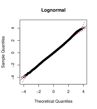
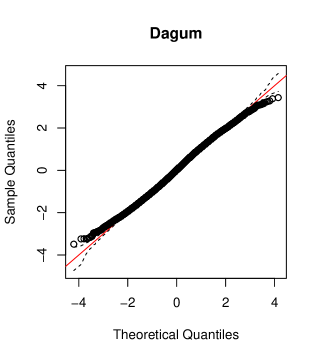
Figure 1: Normal QQ-plots for the univariate income model and different distributions with 95% reference bands.

Variable selection

For the specification of the link function of the ordinal response, as well as variable selection for the bivariate model, and the choice of the copula function, the Akaike’s Information Criterion (AIC) and the Bayesian Information Criterion (BIC) can be used. These are defined as

AIC $$:=-2\ell(\hat{\boldsymbol{\beta}})+2\mathrm{edf},$$

BIC $$:=-2\ell(\hat{\boldsymbol{\beta}})+\log(n)\mathrm{edf},$$

where $\ell(\hat{\boldsymbol{\beta}})$ is the log likelihood of the bivariate model evaluated at the penalized parameter estimate and $\mathrm{edf}=\mathrm{tr}(\hat{\boldsymbol{A}})$ as defined in Section 3.2. Theoretical knowledge about the problem at hand facilitates the variable selection procedure by pre-selecting candidate predictors. Radice et al. (2016) also suggest to start with a model specification where all distributional and the association parameter depend on all covariates. In case the algorithm does not converge, an instance that often indicates that the sample size is too small for the model’s complexity, they recommend trying out a series of more parsimonious specifications. To test smooth components for equality to zero, we have adapted the results of Wood (2017) to the current context.

To fit the bivariate model, we specify an equation for each distributional and the copula parameter as follows: We start with a set of variables selected according to economic reasoning. Note that often in income or expenditure equations, household size is used as a covariate in addition to number of children and elderly. However, we do not wish to separate the child effect in a “pure” child effect and children as additional household member effect. Moreover, the outcome variable is already adjusted for household size. Religion is included because it defines minority groups. While education on the individual level is part of the response vector, the level of education of the household head is included as a control in the predictor for capita income. For the bivariate model, we fit a full specification for the location parameter of each marginal distribution, i.e. ${\mu_{1}}_{educ}$ and ${\mu_{2}}_{inc}$ and perform variable selection using the AIC for the scale parameter of the second marginal, ${\sigma_{2}}_{inc}$, and for the copula parameter, ${\gamma}$. More specifically, a backwards selection procedure is applied for ${\sigma_{2}}_{inc}$ given a full specification for ${\gamma}$ and then a second backwards selection is performed on ${\gamma}$ given the reduced model for ${\sigma_{2}}_{inc}$. This excludes only four variables for the scale predictor and two variables for the copula parameter specification, i.e. we arrive at:

$$\eta^{\mu_{1}}_{educ} =\theta_{r}-\{s(age)+\beta^{\mu_{1}}_{1}\cdot hhmarstat+\beta^{\mu_{1}}_{2}\cdot hhmale+\beta^{\mu_{1}}_{3}\cdot urban+$$

$$\quad\,\beta^{\mu_{1}}_{4}\cdot num\_child+\beta^{\mu_{1}}_{5}\cdot elderly+\beta^{\mu_{1}}_{6}\cdot relig\}$$

$$\eta^{\mu_{2}}_{inc} =\beta^{\mu_{2}}_{0}+s(age)+\beta^{\mu_{2}}_{1}\cdot hhmarstat+\beta^{\mu_{2}}_{2}\cdot hhmale+\beta^{\mu_{2}}_{3}\cdot urban+$$

$$\quad\,\beta^{\mu_{2}}_{4}\cdot num\_child+\beta^{\mu_{2}}_{5}\cdot elderly+\beta^{\mu_{2}}_{6}\cdot relig+\beta^{\mu_{2}}_{7}\cdot hheduc+s(prov)$$

$$\eta^{\sigma_{2}}_{inc} =\beta^{\sigma_{2}}_{0}+s(age)+\beta^{\sigma_{2}}_{1}\cdot hhmarstat+\beta^{\sigma_{2}}_{2}\cdot num\_child+\beta^{\sigma_{2}}_{3}\cdot relig+s(prov)$$

$$\eta^{\gamma} =\beta^{\gamma}_{0}+s(age)+\beta^{\gamma}_{1}\cdot hhmarstat+\beta^{\gamma}_{2}\cdot urban+$$

$$\quad\,\beta^{\gamma}_{3}\cdot num\_child+\beta^{\gamma}_{4}\cdot elderly+\beta^{\gamma}_{5}\cdot hheduc+s(prov).$$

Continuous variables enter the equations with smooth non-parameteric effects s() represented via thin plate regression splines with ten bases and second order derivative penalties. Spatial effects of the provinces and their neighbourhood structure are modeled using Markov random fields. We choose to model the spatial effect at the province level since minimum wages are set at the province level affecting individual wages and thus expenditure measure as well (Hohberg and Lay, 2015).

Ordinal model

The ordinal outcome education is fitted using an ordered model. Table 1 compares the AIC and BIC between a probit and a logit link of the bivariate model using the lognormal as the continuous marginal and a Gaussian copula. Both AIC and BIC favor the logit model for the first marginal.

Table 1: AIC and BIC of bivariate ordered-continuous model using the logit and probit links.

	AIC	BIC
logit	1,075,191	1,076,241
probit	1,075,588	1,076,637

Choice of the copula

For the copula selection, a good starting point would be the use of a Gaussian copula and then consider all consistent alternatives depending on the direction of the dependence (Radice et al., 2016; Klein et al., 2019). Again, AIC and BIC can help choosing among several candidate copulas.

Starting off with the Gaussian yields an average value for the copula parameter (with 95% confidence interval in brackets) of $\gamma=0.163\leavevmode\nobreak\ (0.104,0.221)$. Building on this finding, we test a range of suitable possible candidates. After checking convergence, we can only eliminate the un-rotated Joe and Clayton copula. The remaining candidates are compared using the AIC and BIC; see Table 2 for the results. The AIC and BIC indicate that a Gaussian copula should be used for our model, and all copula models should be favoured over the independence model. Using the Gaussian copula suggests that the dependence between per capita expenditures and education is symmetric with asymptotically independent extremes.

Table 2: AIC and BIC for different copula specifications.

	AIC	BIC
Gaussian	1,075,191	1,076,241
F	1,075,233	1,076,295
FGM	1,075,280	1,076,335
PL	1,075,226	1,076,286
AMH	1,075,298	1,076,359
C0	1,075,448	1,076,508
C180	1,075,379	1,076,380
J0	1,075,514	1,076,462
J180	1,075,516	1,076,573
G0	1,075,351	1,076,360
G180	1,075,306	1,076,341
Independence	1,075,892	1,076,678
Note: Abbreviations correspond to Frank, Farlie-Gumbel-Morgenstern, Plackett, Ali-Mikhail-Haq, Clayton, rotated Clayton (180 degrees), Joe, rotated Joe (180 degrees), Gumbel, rotated Gumbel (180 degrees), respectively.

4.3 Model evaluation

After deciding on the marginal distributions, the copula and covariates by comparing different candidates, we check the final bivariate model. To this end, we use a multivariate generalization of the quantile residuals introduced in Section 4.2 that was proposed by (Kalliovirta, 2008). Multivariate quantile residuals for two continuous responses are defined as

$$\hat{\boldsymbol{q}}_{i}=\begin{pmatrix}\hat{q}_{1i}\\ \hat{q}_{2i}\end{pmatrix}=\begin{pmatrix}\Phi^{-1}(\hat{F}_{1}(y_{1i}))\\ \Phi^{-1}(\hat{F}_{2|1}(y_{2i}|y_{1i})),\end{pmatrix}$$

where $\hat{F}_{2|1}$ is the (estimated) conditional CDF of $Y_{2}$ given $Y_{1}$. In our case, the first marginal is discrete such that we resort to randomized quantile residuals where uniformly distributed random variables on the interval corresponding to cumulated probabilities are plugged into $\Phi^{-1}(\cdot)$. If the model is correctly specified, then $\hat{\boldsymbol{q}}$ approximately follows a bivariate standard normal distribution.

The contour plot for the bivariate model in Figure 2(a) shows the density of the quantile residuals $\hat{\boldsymbol{q}}$ by means of a multivariate kernel density estimator. This estimated density is compared to the density of the standard normal distribution. The contour lines of both densities are close to each other indicating a good fit of the bivariate copula model.

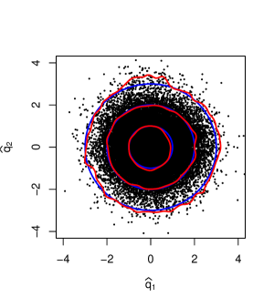
(a) Contour plot of multivariate quantile residuals. The red lines indicate the density of the quantile residuals estimated by a multivariate kernel density estimator. The blue circles are the contour lines of the density of the standard normal distribution with radius $1,2$ and $3$.

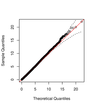
(b) QQ-plot depicting the sum of the squared elements of the multivariate quantile residuals with 95% reference bands.

Figure 2: Multivariate quantile residuals of the bivariate model.

In Figure 2(b), the sum of the squared elements of the multivariate quantile residuals are considered. That is, $\hat{\boldsymbol{q}}_{i}^{\prime}\hat{\boldsymbol{q}}_{i}=\hat{q}_{1i}^{2}+\hat{q}_{2i}^{2},$ where $\hat{\boldsymbol{q}}_{i}$ is the multivariate quantile residual for the $i$-th individual. Since $\hat{q}_{1i}\stackrel{{\scriptstyle a}}{{\sim}}\mathcal{N}(0,1)$ and $\hat{q}_{2i}\stackrel{{\scriptstyle a}}{{\sim}}\mathcal{N}(0,1)$, it follows that $\hat{\boldsymbol{q}}_{i}^{\prime}\hat{\boldsymbol{q}}_{i}\stackrel{{\scriptstyle a}}{{\sim}}\chi^{2}(2)$ which is assessed in the QQ-plot in Figure 2(b). The reference bands are obtained by repeatedly simulating from a $\chi^{2}(2)$ distribution. We draw $n_{rep}=100$ samples and compute the $2.5\%$ and $97.5\%$ quantiles for each observations across the sorted $n_{rep}$ samples. The plot supports our model choice.

4.4 Results

This section demonstrates the results that poverty researchers can derive from fitting a copula GAMLSS model for the joint analysis of two inter-related poverty dimensions. We summarise briefly the covariate effects on the marginals before taking a closer look at the dependence structure and risk groups. This way, we are able to answer questions on how dependence and risk are affected by a household’s location or composition.

Effects of covariates on the marginal distributions

The full list of effects on each parameter of the marginals and on the copula parameter is included in the Appendix F. Note that the effects are subject to a ceteris paribus interpretation. For example, more schooling is associated with more income with tertiary education having the highest effect. Households with more children or elderly people living in the household have on average a lower income per capita and less education (except for the effect of one elderly on education which is negative and not statistically significant). Urban households are associated with both better income and better education. A little surprising is that living in a household where the head is married is correlated with a reduction in income and education compared to not (yet) married households (Table 7 and 6). One possible explanation is that non-married households compared to married households include a larger share of young, single persons that do not need to share their income and have a comparatively higher level of education. Non-Muslim households are associated with higher income per capita and more education although they represent a minority in Indonesia. For a male household head, the effects are not as expected since it is negative for income but positive for education. For the second parameter of the continuous margin, i.e. the scale parameter for the income equation, the number of children and a marital status other than not married have negative effects while the effects of elderly and other religions compared to Islam are positive. All of the covariates have a positive effect on the copula parameter though not all effects are significant.

Age is modeled in a non-linear way and Figure 3 displays the smooth effects of age on each parameter. Education attainments are lower for higher ages which can be explained by the education expansion that Indonesia has undergone since the 1970’s and younger individuals benefited from. For example, between 1974 and 1978 over 61,000 primary schools were built. In 1984, compulsory education was set to six years which was extended to nine years in 1994 (Akita, 2017; Duflo, 2004). The effect of income on the location parameter is inverted u-shaped until the age of 60 with a peak around the age of 40. After 80, the confidence intervals become very wide due to a lower number of observations in this age span and the effect is thus less clear. The effects on the scale parameter are around zero. For the copula parameter, the age effect indicates that the dependence is decreasing for individuals up to their mid 30ies and stays around zero afterwards until it decreases again after the age of 60.

Figure 3: Estimated smooth functions of age and respective point-wise 95% confidence intervals.

Figure 4 shows the effect of the underlying spatial pattern on the parameters $\mu_{2}$ and $\sigma_{2}$ of the second response, and on the copula parameter $\gamma$. Households located in provinces of Java seem to have higher income per capita compared to the observed provinces in Sumatra, Borneo and Sulawesi. Provinces with a negative effect on the location parameter have higher effects on the scale parameter except for Borneo whose scale effect is negative.

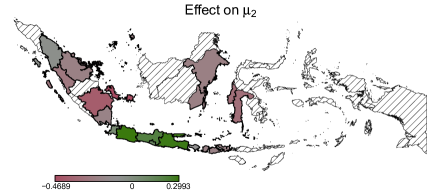
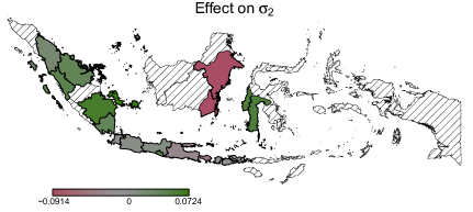
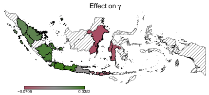
Figure 4: Spatial effects of the provinces on the distribution parameters of income and on the copula parameter.

Dependence structure

When focusing on the dependence, its structure can be represented via contour plots for specific covariate combinations. For example, we focus here on the location of the household (urban/rural and province) as they are the significant drivers of the copula parameter, while the remaining plots can be found in Appendix F. For comparison purposes, we include provinces with the highest frequencies in the dataset but select only one of Java’s provinces. To compare the dependence structure across different locations, we create an example of typical individual whose characteristics, other than the one under consideration, are set to their mean value or to their most frequent observation. The only exception is the education of the household head which is set to the second most frequent observation. For a household head with "high school" degree the dependence is a bit more pronounced we hence selected this level for demonstration purposes. This is the covariates’ combination that we call an “example individual” henceforward.

Figure 5(a) shows that the dependence is stronger for individuals in urban households compared to rural households. One reason might be that average education levels are lower in rural areas (x-axis) while at the same time high paid job opportunities are restricted in a rural environment, resulting in more equal incomes compared to an urban environment. Figure 5(b) compares the dependence structure across selected provinces. The dependence seems weakest in the province of Nusa Tenggara Barat, which is one of the poorest provinces in Indonesia. It is surprising that the average per capita consumption (straight line) of Jakarta is about the same level than that one of Nusa Tenggara Barat. Most likely this is due to the high price level in Jakarta and the deflation measure applied which scaled down our expenditure measure maybe too drastically. Though the copula coefficient for Jakarta is similar to Jawa Timur, the latter has more variation in incomes and the contour levels lie further apart. Considering all – and not just the selected provinces – the value of the copula parameter for the example individual ranges from 0.16 for Kalimantan Timur and Kalimantan Selatan up to 0.27 for Yogyakarta.

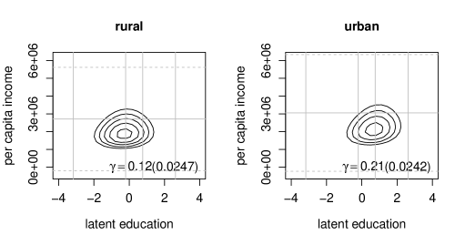
(a) Contour plots for an example individual in an urban or rural household in the province of Jawa Timur.

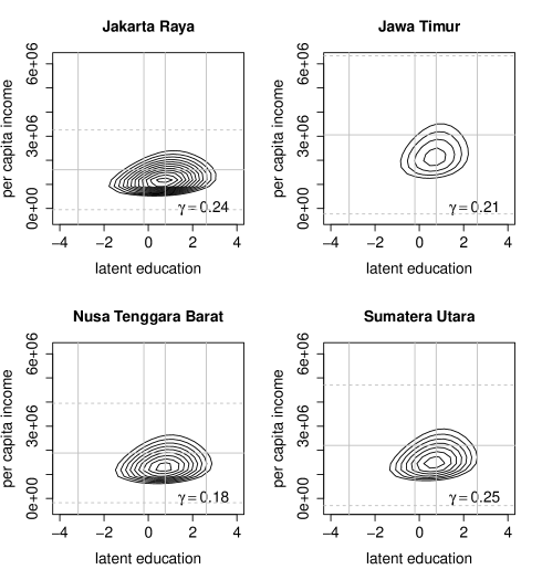
(b) Contour plots for an example individual in an urban household in different provinces.

Figure 5: Contour plots for (education, income)’ and a Gaussian copula by households’ location. Contour lines of densities are at levels from 0.00000005 to 0.00000025 in 0.00000001 steps. The vertical straight lines represents the cut off values for the education categories, horizontal straight lines are the consumption average, and dashed horizontal line are at two standard deviations around this average.

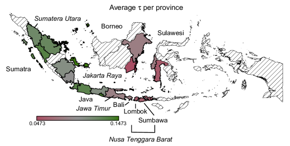
Figure 6: Kendall’s $\tau$ for each individual averaged within provinces.

A policy maker might be interested to know in which locations each individual in the dataset, and not the example individual, have higher dependencies in order to efficiently design policy strategies. Although the lower panel of Figure 4 shows the effect of the provinces on the copula parameter, it might be more helpful for interpretation to transform it into the Kendall’s $\tau$, an association measure that takes on values on $[-1,1]$. Each individual with his/her specific covariates’ combination is related to an individual-specific $\tau$. One way to present the differences across provinces is to average the $\tau$ over all individuals in a particular province. This is shown in Figure 6. The Kalimantan Selatan (South Borneo) is the province with the lowest average of Kendall’s $\tau$ with a value of 0.0468 and Kepulauan Riau (Riau Islands, northwest of Borneo) has a value of 0.1467 which is the highest average value that also indicates spatial heterogeneity in the strength of the dependence. The provinces of Sumatra seem to have higher dependence between income and education than provinces in Borneo or Sulawesi. Interestingly, for Java and its neighbouring smaller islands on the east, the dependence seem to decrease from west to east.

Joint probabilities

Other results we can derive from a copula GAMLSS models are joint probabilities for different sub-groups. That is, we calculate the probability for the example individual of being poor in both the education and income dimensions. As an example, we again focus here on household location and additionally consider household composition. To define poverty, we classify individuals that have only primary or even less education as education poor and set a relative poverty line of 60% of the median of unique values of per capita expenditures. Note that Indonesia also has a national absolute poverty line that is, however, based on a different expenditure measure than the one we constructed from the IFLS data. We thus decided to use a relative poverty line. An individual that is poor in both dimensions has expected values below each of these thresholds. One of the sub-groups is set to one and the probability of the other sub-group is compared to this base category. Figure 7 shows that the probability for being poor in both dimensions is 2 times higher for the example individual in a rural household compared to the same individual in an urban household. Compared to Jawa Timur the joint probabilities of Jakarta Raya, Nusa Tenggara Barat, and Sumatera Utara are about 8 times, 6 times, and 4 times higher, respectively. Not surprisingly, the risk of being poor in both dimensions increases with the number of children and elderly in the household.

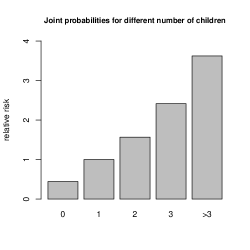
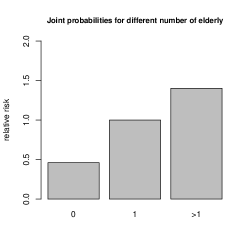
Figure 7: Relative joint poverty risks of an example individual differentiated by household location and household composition. Baseline categories are urban, Jawa Timur, 1 child, and 1 elderly, respectively, and are set to one. The abbreviation NTB denotes the province of Nusa Tenggara Barat.

Vulnerability to poverty

The higher the dependence between education and income, the higher the chances that we miss some individuals at risk by only looking at the marginal distributions of each poverty dimension. To identify the individuals at risk, we calculate the probabilities of being poor in two dimensions for each individual in the dataset, first for the independence model and then for the copula model. A vulnerability threshold is arbitrarily defined at a probability of 0.1 for simplicity. All individuals with a probability of being poor above this threshold are declared as vulnerable. We then compare the individuals that are identified as vulnerable by the copula and the independence models to their actual poverty status and calculate the specificity or true positive rate. Results are displayed in Table 3. We find that the copula model has better specificity for two-dimensional poverty than the independence model although the difference is fairly small.

Table 3: Specificity of the copula and independence models. Individuals that are declared vulnerable are compared to their actual poverty status.

	copula	independence
income dimension	0.88	0.88
both dimensions	0.66	0.63

Discussion of Results

The main advantage of applying copula GAMLSS in the precedent poverty analysis is that we are able to analyse the dependence between poverty dimensions in more detail than studies that are limited to measuring the dependence. Even though the dependence is not very strong, once we control for covariates in the marginals, we consider this an interesting outcome. We could further identify heterogeneities in the strength of the dependence between income and education, and poverty risk with respect to a household’s location. For example, an example individual in a rural household exhibit lower dependencies compared to the same individual in an urban household. One explanation might be that opportunities in rural areas are restricted and thus the individual’s education level has a smaller influence on per capita expenditures.

There is also a strong spatial heterogeneity between provinces. High dependencies can be found in the northwest while the values decrease for the more central provinces. The explanation for low dependence due to low opportunities could also apply to the province of Nusa Tenggara Barat which showed little average dependence and lower dependence for a specific example individual compared to other provinces. Nusa Tenggara Bararat is one of the poorest provinces, with a low GDP per capita and with agriculture and fishery being the most important industries. On the other hand, provinces such as Jakarta and Kalimantan Timur, that have the highest per capita GDP out of all provinces in Indonesia, have higher probabilities of being poor in both dimensions compared to most other provinces. These probabilities are calculated for an example individual that have average characteristics and a high school degree. Possible reasons for the discrepancy between rich provinces and high relative poverty risks might be that in Jakarta income and consumption are very unequally distributed and in East Kalimantan the high GDP is a result of high natural resource exploitation which yields little benefit for the population (see for example Bhattacharyya and Resosudarmo, 2015, who found that growth in the mining sector has had no effect on poverty and inequality in Indonesia).

5 Conclusion

Though poverty is conventionally regarded a multidimensional phenomenon, regression analyses in the poverty context either examine dimensions separately or use a scalar index such as the Multidimensional Poverty Index as an outcome. Both approaches neglect the dependence between poverty dimensions. This paper presents an alternative model for an in-depth poverty study that explicitly analyses this dependence and its determinants. It is important to understand what drives the dependence between poverty dimensions since high dependencies can explain persisting poverty.

For this type of poverty analysis, we propose the use of bivariate copula GAMLSS which relate each distributional parameter of the marginals and of the copula parameter to flexible covariate effects. Since poverty analyses often include one monetary measure such as income or consumption and some ordinal measure such as education level or health status, we extended the class of copula GAMLSS to incorporate ordinal data based on a latent variable approach. This extension has been incorporated in the GJRM R-package.

We use data from Indonesia to show how copula GAMLSS can be applied to a poverty analysis. The model identified the number of elderly and children in the household, the education of the household head, and the household’s location as risk factors for low income or poor education or both, and the probability of being poor in both dimensions. The gender of the household head, belonging to a minority religion and being widowed or separated compared to being married, has shown less or the opposite influence than expected. We did not find evidence for strong tail dependencies between education and expenditures after conditioning on the covariates in the marginals and in the copula parameter.

Focusing more on the household’s location, we find that an example individual in a rural household exhibits lower dependencies compared to the same individual in an urban household, potentially due to restricted employment opportunities for highly educated individuals in rural areas. There is a strong spatial heterogeneity regarding poverty risk and the strength of the dependence. High dependencies can be found in the northwest of Indonesia while central provinces have lower ones. For Jakarta and Kalimantan Timur we found a discrepancy between being rich in terms of GDP and exhibiting high relative poverty risks, potentially indicating unequally distributed economic gains.

Thanks to the flexibility of our approach, the analysis of the dependence between poverty dimensions, and the various results that can be derived consistently by only estimating one model, we advocate to include copula GAMLSS into the tool box of poverty researchers. Other applications in the context of poverty may include analysing the drivers and spatial patterns of inter-generational poverty persistence or upward social mobility. On the methodological side, future research can be directed at combining copula GAMLSS with experimental or quasi-experimental methods to evaluate Indonesia’s poverty policies on the micro level. Extensions beyond the bivariate case are dependent on the availability of a suitable copula. The implementation of these models subsequently becomes more numerically and technically demanding and interpretation of the regression results will be challenging.

Appendix A Considered copulas and corresponding (transformed) parameter

Table 4: Families of some bivariate copula functions.

Name	$\mathcal{C}(u,v)$	range of $\gamma$	$\gamma^{*}$	Kendall’s $\tau$
Gaussian	$\Phi_{2}(\Phi^{-1}(u),\Phi^{-1}(v))$	$[-1,1]$	$\textup{tanh}^{-1}(\gamma)$	$\frac{2}{\pi}\arcsin{\gamma}$
Clayton	$(u^{-\gamma}+v^{-\gamma}-1)^{-1/\gamma}$	$(0,\infty)$	$\log(\gamma-\varepsilon)$	$\frac{\gamma}{\gamma+2}$
Frank	$-\gamma^{-1}\log[1+(e^{-\gamma u}-1)(e^{-\gamma v}-1)/(e^{-\gamma}-1)]$	$\mathds{R}\setminus\{0\}$	$\gamma-\varepsilon$	$1-\frac{4}{\gamma}(1-D_{1}(\gamma))$
Gumbel	$\exp\left\{-[(-\log u)^{\gamma}+(-\log v)^{\gamma}]^{1/\gamma}\right\}$	$[1,\infty)$	$\log(\gamma-1)$	$1-\frac{1}{\gamma}$
Joe	$1-[(1-u)^{\gamma}+(1-v)^{\gamma}-(1-u)^{\gamma}(1-v)^{\gamma}]^{1/\gamma}$	$(1,\infty)$	$\log(\gamma-1-\varepsilon)$	$1+\frac{4}{\gamma^{2}}D_{2}(\gamma)$
FGM	$uv[1+\gamma(1-u)(1-v)]$	$[-1,1]$	$\textup{tanh}^{-1}(\gamma)$	$\frac{2}{9}\gamma$
AMH	$\frac{uv}{1-\gamma(1-u)(1-v)}$	$[-1,1)$	$\textup{tanh}^{-1}(\gamma)$	$1-\frac{2}{3\gamma^{2}}(\gamma+(1-\gamma)^{2}\log(1-\gamma))$
Plackett	$\frac{1+(\gamma-1)(u+v)-\sqrt{[1+(\gamma-1)(u+v)]^{2}-4\gamma(\gamma-1)uv}}{2(\gamma-1)}$	$(0,\infty)$	$\log(\gamma-\varepsilon)$	-
Note: The association parameter is denoted by $\gamma$ and $u$ and $v$ are the marginals $F_{1}(\eta_{1k})$ and $F_{2}(y_{2})$, respectively. The abbreviations FGM and AMH correspond to the Farlie-Gumbel-Morgenstern and the Ali-Mikhail-Haq copula, respectively. Function $\Phi_{2}(\dot{,}\dot{;}\gamma)$ is the CDF of a bivariate standard normal distribution, while $D_{1}(\gamma)=\frac{1}{\gamma}\int_{0}^{\gamma}\frac{t}{\exp(t)-1}dt$ is the Debye function and $D_{2}(\gamma)=\int_{0}^{1}t\log(t)(1-t)^{\frac{2(1-\gamma)}{\gamma}}dt$ . The quantity $\varepsilon$ denotes the machine smallest floating point multiplied by $10^{6}$ and is introduced to force the transformed association parameters to lie in their respective supports throughout estimation.

Appendix B Further details on the trust algorithm and smoothing parameter selection

B.1 General idea of the trust region algorithm

The trust region algorithm has the advantage of being more stable and faster compared to in-line search methods (Marra and Radice, 2017). Both line search and trust region methods use a quadratic model of the objective function and generate steps from one iterate to the next. While line search methods use the model to find first a search direction and suitable step lengths along this direction, trust region algorithms search the step that minimizes the objective function within a previously defined region around the current iterate such that both direction and step length are selected at the same time. If a function exhibits long plateaus and the current iterate $\boldsymbol{\beta}^{[a]}$ is in that region, line search methods may search the next step $\boldsymbol{\beta}^{[a+1]}$ far away from the current iterate. In this case, it is possible that the evaluation of the log likelihood will not be finite causing the algorithm to fail. Before evaluating the objective function, trust region methods define a maximum distance first based on the trust region. This has two advantages: first, the new iterate will not lie too far away from the current one; second, in case of a non-definite evaluation of $\breve{\ell}_{p}$, step $\boldsymbol{p}^{[a+1]}$ will be rejected. If a candidate that minimizes the quadratic approximation of the objective function and also lies in the trust region does not improve the function sufficiently or gives a non definite evaluation of $\breve{\ell}_{p}$, the trust region shrinks and the algorithm moves back to step 1. On the other hand, if the improvement is large enough, the trust region expands in the next iteration. Details on the trust region algorithm can be found in Nocedal and Wright (2006), Chapter 4.

B.2 Details on smoothing parameter selection

Simultaneous optimization of $\boldsymbol{\beta}$ and $\boldsymbol{\lambda}$ causes overfitting. The reason is that the penalized log-likelihood will be highest at $\boldsymbol{\lambda}=\boldsymbol{0}$. Instead, the smoothing parameters $\boldsymbol{\lambda}$ should be selected in a way such that the function estimates are close to the true functions.

Providing a full justification, Marra et al. (2017) propose an approach that yields the result in equation (10). They use the fact that, close to convergence, the trust region algorithm behaves like a classic unconstrained algorithm (Radice et al., 2016). Considering the first order Taylor expansion of $\boldsymbol{g}_{p}^{[a+1]}$ and setting this to zero, they obtain

$$\boldsymbol{0}=\boldsymbol{g}_{p}^{[a+1]}\approx\boldsymbol{g}_{p}^{[a]}+\boldsymbol{H}_{p}^{[a]}(\boldsymbol{\beta}^{[a+1]}-\boldsymbol{\beta}^{[a]}),$$ (11)

where the quantities as those defined in the paper. The aim is now to find an expression for $\boldsymbol{\beta}^{[a+1]}$ that uses $\boldsymbol{g}^{[a]}$ and $\boldsymbol{H}^{[a]}$ as a whole. Marra et al. (2017) argue that this reduces the frequency of situations where $\boldsymbol{H}$ is not positive definite compared to when working with the $n$ components that make it up. The situations where $\boldsymbol{H}$ turns out not to be positive definite can then be dealt with by perturbing $\boldsymbol{H}$ to positive definiteness (Wood, 2015). Recalling that $\boldsymbol{\cal I}^{[a]}=-\boldsymbol{H}^{[a]}$, the expression in (11) can be re-written as

$$\boldsymbol{0} =\boldsymbol{g}_{p}^{[a]}+(-\boldsymbol{\cal{I}}^{[a]}-\boldsymbol{S}_{\boldsymbol{\lambda}})(\boldsymbol{\beta}^{[a+1]}-\boldsymbol{\beta}^{[a]})$$

$$\boldsymbol{g}_{p}^{[a]} =(\boldsymbol{\cal{I}}^{[a]}+\boldsymbol{S}_{\boldsymbol{\lambda}})(\boldsymbol{\beta}^{[a+1]}-\boldsymbol{\beta}^{[a]})$$

$$\boldsymbol{g}^{[a]}-\boldsymbol{S}_{\boldsymbol{\lambda}}\boldsymbol{\beta}^{[a]} =(\boldsymbol{\cal{I}}^{[a]}+\boldsymbol{S}_{\boldsymbol{\lambda}})(\boldsymbol{\beta}^{[a+1]})-(\boldsymbol{\cal{I}}^{[a]}+\boldsymbol{S}_{\boldsymbol{\lambda}})(\boldsymbol{\beta}^{[a]})$$

$$(\boldsymbol{\cal{I}}^{[a]}+\boldsymbol{S}_{\boldsymbol{\lambda}})\boldsymbol{\beta}^{[a+1]} =\boldsymbol{g}^{[a]}-\boldsymbol{S}_{\boldsymbol{\lambda}}\boldsymbol{\beta}^{[a]}+(\boldsymbol{\cal{I}}^{[a]}+\boldsymbol{S}_{\boldsymbol{\lambda}})\boldsymbol{\beta}^{[a]}$$

$$=\boldsymbol{g}^{[a]}+\boldsymbol{\cal{I}}^{[a]}\boldsymbol{\beta}^{[a]}$$

$$\boldsymbol{\beta}^{[a+1]} =(\boldsymbol{\cal{I}}^{[a]}+\boldsymbol{S}_{\boldsymbol{\lambda}})^{-1}\sqrt{\boldsymbol{\cal{I}}^{[a]}}(\sqrt[]{\boldsymbol{\cal{I}}^{[a]}}\boldsymbol{\beta}^{[a]}+\sqrt[]{\boldsymbol{\cal{I}}^{[a]}}^{-1}\boldsymbol{g}^{[a]}).$$

Thus, at convergence the parameter estimator takes the following form

$$\boldsymbol{\beta}^{[a+1]}=(\boldsymbol{\cal I}^{[a]}+\boldsymbol{S}_{\boldsymbol{\lambda}})^{-1}\sqrt{{\boldsymbol{\cal I}}^{[a]}}\boldsymbol{M}^{[a]},$$

where $\boldsymbol{M}^{[a]}:=\boldsymbol{\mu_{M}}^{[a]}+\boldsymbol{\epsilon}^{[a]}$, $\boldsymbol{\mu_{M}}^{[a]}:=\sqrt{\boldsymbol{\cal I}^{[a]}}\boldsymbol{\beta}^{[a]}$ and $\boldsymbol{\epsilon}^{[a]}:=\sqrt{\boldsymbol{\cal I}^{[a]}}^{-1}\boldsymbol{g}^{[a]}$.

From likelihood theory we have that $\boldsymbol{\epsilon}\sim{\cal N}(\boldsymbol{0},\boldsymbol{I})$ and $\boldsymbol{M}\sim{\cal N}(\boldsymbol{\mu}_{\boldsymbol{M}},\boldsymbol{I})$, with $\boldsymbol{I}$ being the identity matrix and $\boldsymbol{\mu}_{\boldsymbol{M}}:=\sqrt{\boldsymbol{\cal{I}}}{\boldsymbol{\beta}^{0}}$, where $\boldsymbol{\beta}^{0}$ denotes the true parameter vector. The predicted value vector for $\boldsymbol{M}$ is $\hat{\boldsymbol{\mu}}_{\boldsymbol{M}}=\sqrt[]{\boldsymbol{\cal I}}\hat{\boldsymbol{\beta}}=\boldsymbol{AM}$, where $\boldsymbol{A}=\sqrt{\boldsymbol{\cal I}}(\boldsymbol{\cal I+\boldsymbol{S}_{\boldsymbol{\lambda}}})^{-1}\sqrt{\boldsymbol{\cal I}}$. To obtain an estimate of $\boldsymbol{\lambda}$ that suppresses the complexity of smooth terms not supported by the observed data, $\hat{\boldsymbol{\mu}}_{\boldsymbol{M}}$ should be close to $\boldsymbol{\mu}_{\boldsymbol{M}}$. Hence, employing the expected squared error, yields

$$\mathbb{E}(\|\boldsymbol{\mu_{M}}-\hat{\boldsymbol{\mu}}_{\boldsymbol{M}}\|^{2}) =\mathbb{E}(\|(\boldsymbol{M}-\boldsymbol{\epsilon})-\boldsymbol{AM}\|^{2})$$

$$=\mathbb{E}(\|\boldsymbol{M}-\boldsymbol{AM}-\boldsymbol{\epsilon}\|^{2})$$

$$=\mathbb{E}(\|\boldsymbol{M}-\boldsymbol{AM}\|^{2})+\mathbb{E}(-\boldsymbol{\epsilon}^{\prime}\boldsymbol{\epsilon}-2\boldsymbol{\epsilon}^{\prime}\boldsymbol{\mu_{M}}+2\boldsymbol{\epsilon}^{\prime}\boldsymbol{A\mu_{M}}+2\boldsymbol{\epsilon}^{\prime}\boldsymbol{A\epsilon})$$

$$=\mathbb{E}(\|\boldsymbol{M}-\boldsymbol{AM}\|^{2})-Kn+2\textrm{tr}(\boldsymbol{A}).$$ (12)

The smoothing parameter is found by minimizing an estimate of the expectation in equation (12). For a given $\boldsymbol{\beta}^{[a+1]}$ we arrive then at equation (10).

Appendix C Gradient and Hessian

Throughout the derivations of the gradient vector and the Hessian matrix, we denote by $\boldsymbol{\beta}_{1}$ the regression coefficient associated to the fist ordinal equation, and by $\boldsymbol{\beta}_{2}:=(\boldsymbol{\beta}^{\mu_{2}},\boldsymbol{\beta}^{\sigma_{2}})^{\prime}$ the coefficients for the location and scale parameters of the second continuous equation. Similarly $\boldsymbol{\beta}^{\gamma}$ refers to the coefficients of the copula association parameter.

C.1 Gradient vector

A general expression for the contribution of the $i$-th individual to the gradient vector is the following

$$\ell_{\boldsymbol{\beta}i}^{\prime}(\boldsymbol{\beta}):=\frac{\partial\ell_{i}(\boldsymbol{\beta})}{\partial\boldsymbol{\beta}}=\sum_{r\in\mathcal{R}}\mathds{1}_{\{y_{1i}=r\}}\frac{1}{\nabla_{r}F_{12.2}(\eta_{1ri})}\frac{\partial\nabla_{r}F_{12.2}(\eta_{1ri})}{\partial\boldsymbol{\beta}}+f_{2}(y_{2i})^{-1}\frac{\partial f_{2}(y_{2i})}{\partial\boldsymbol{\beta}},$$

where $\nabla_{r}$ is the backward difference operator applied to $r$, in particular $\nabla_{r}F_{12.2}(\eta_{1ri}):=F_{12.2}(\eta_{1ri})-F_{12.2}(\eta_{1r-1i})$. We next define the quantities

$$F_{12.12}(\eta_{1ri}):=\frac{\partial^{2}\mathcal{C}(F_{1}(\eta_{1ri}),F_{2}(y_{2i}))}{\partial F_{1}(\eta_{1ri})\partial F_{2}(y_{2i})}\qquad\textrm{with}\qquad F_{12.22}(\eta_{1ri}):=\frac{\partial^{2}\mathcal{C}(F_{1}(\eta_{1ri}),F_{2}(y_{2i}))}{\partial F_{2}(y_{2i})^{2}}.$$

C.1.1 Derivatives with respect to the transformed cut points

• $h=1$:

  $$\ell_{\theta_{1}^{*}i}^{\prime} =\frac{1}{\nabla_{r}F_{12.2}(\eta_{1ri})}\frac{\partial\theta_{1}}{\partial\theta_{1}^{*}}\left(F_{12.12}(\eta_{1ri})\frac{\partial F_{1}(\eta_{1ri})}{\partial\eta_{1ri}}\frac{\partial\eta_{1ri}}{\partial\theta_{1}}-F_{12.12}(\eta_{1r-1i})\frac{\partial F_{1}(\eta_{1r-1i})}{\partial\eta_{1r-1i}}\frac{\partial\eta_{1r-1i}}{\partial\theta_{1}}\right)$$

  $$=\frac{1}{\nabla_{r}F_{12.2}(\eta_{1ri})}\left(F_{12.12}(\eta_{1ri})f_{1}(\eta_{1ri})-\mathds{1}_{\{2\preceq r\}}F_{12.12}(\eta_{1r-1i})f_{1}(\eta_{1r-1i})\right)$$

• $h=2,\ldots,R$:

  $$\ell_{\theta_{h}^{*}i}^{\prime} =\frac{1}{\nabla_{r}F_{12.2}(\eta_{1ri})}\frac{\partial\theta_{h}}{\partial\theta_{h}^{*}}\left(F_{12.12}(\eta_{1ri})\frac{\partial F_{1}(\eta_{1ri})}{\partial\eta_{1ri}}\frac{\partial\eta_{1ri}}{\partial\theta_{h}}-F_{12.12}(\eta_{1r-1i})\frac{\partial F_{1}(\eta_{1r-1i})}{\partial\eta_{1r-1i}}\frac{\partial\eta_{1r-1i}}{\partial\theta_{h}}\right)$$

  $$=\frac{2}{\nabla_{r}F_{12.2}(\eta_{1ri})}\left(\mathds{1}_{\{h\preceq r\}}F_{12.12}(\eta_{1ri})f_{1}(\eta_{1ri})-\mathds{1}_{\{h+1\preceq r\}}F_{12.12}(\eta_{1r-1i})f_{1}(\eta_{1r-1i})\right)\theta_{h}^{*}$$

C.1.2 Derivatives with respect to $\boldsymbol{\beta}_{1}$ and $\boldsymbol{\beta}_{2}$

• $\boldsymbol{\beta}_{1}$:

  $$\ell_{\boldsymbol{\beta}_{1}i}^{\prime} =\left[\frac{1}{\nabla_{r}F_{12.2}(\eta_{1ri})}\nabla_{r}\left(\frac{\partial F_{1}(\eta_{1ri})}{\partial\eta_{1ri}}\frac{\partial F_{12.2}(\eta_{1ri})}{\partial F_{1}(\eta_{1ri})}\right)\right]\frac{\partial\eta_{1ri}}{\partial\boldsymbol{\beta}_{1}}$$

  with $$\quad\frac{\partial\eta_{1ri}}{\partial\boldsymbol{\beta}_{1}}=\frac{\partial\eta_{1r-1i}}{\partial\boldsymbol{\beta}_{1}}$$

• $\boldsymbol{\beta}_{2}$; $\vartheta_{k}=\{\mu_{2},\sigma_{2}\}$:

  $$\ell_{\boldsymbol{\beta}_{2}i}^{\prime}\, =\left[\frac{1}{\nabla_{r}F_{12.2}(\eta_{1ri})}\nabla_{r}\left(\frac{\partial F_{12.2}(\eta_{1ri})}{\partial F_{2}(y_{2i})}\right)\frac{\partial F_{2}(y_{2i})}{\partial\vartheta_{k}}+f_{2}(y_{2i})^{-1}\left.\frac{\partial f_{2}(y_{2i})}{\partial\vartheta_{k}}\right]\frac{\partial\vartheta_{k}}{\partial\eta^{\vartheta_{k}}_{i}}\frac{\partial\eta^{\vartheta_{k}}_{i}}{\partial\boldsymbol{\beta}^{\vartheta_{k}}}\right.$$

C.1.3 Derivatives with respect to the copula association parameter

$$\ell_{\boldsymbol{\beta}^{\gamma}i}^{\prime} =\left[\frac{1}{\nabla_{r}F_{12.2}(\eta_{1ri})}\nabla_{r}\left(\frac{F_{12.2}(\eta_{1ri})}{\partial\gamma}\right)\right]\frac{\partial\gamma}{\partial\eta^{\gamma}_{i}}\frac{\partial\eta^{\gamma}_{i}}{\partial\boldsymbol{\beta}^{\gamma}}$$

C.2 Hessian matrix

The general expression for the contribution of the $i$-th individual to the Hessian matrix is given by

$$\ell_{\boldsymbol{\beta}\boldsymbol{\beta}^{\prime}}^{\prime\prime}(\boldsymbol{\beta}) :=\frac{\partial}{\partial\boldsymbol{\beta}}\left(\frac{\partial\ell_{i}(\boldsymbol{\beta})}{\partial\boldsymbol{\beta}}\right)^{\prime}$$

$$=\sum_{r\in\mathcal{R}}\mathds{1}_{\{y_{1i}=r\}}\frac{1}{\nabla_{r}F_{12.2}(\eta_{1ri})}$$

$$\left[\frac{\partial^{2}\nabla_{r}F_{12.2}(\eta_{1ri})}{\partial\boldsymbol{\beta}\partial\boldsymbol{\beta}^{\prime}}-\frac{1}{\nabla_{r}F_{12.2}(\eta_{1ri})}\left(\frac{\partial\nabla_{r}F_{12.2}(\eta_{1ri})}{\partial\boldsymbol{\beta}}\right)\left(\frac{\partial\nabla_{r}F_{12.2}(\eta_{1ri})}{\partial\boldsymbol{\beta}}\right)^{\prime}\right]$$

$$+f_{2}(y_{2i})^{-1}\frac{\partial^{2}f_{2}(y_{2i})}{\partial\boldsymbol{\beta}\partial\boldsymbol{\beta}^{\prime}}-f_{2}(y_{2i})^{-2}\left(\frac{\partial f_{2}(y_{2i})}{\partial\boldsymbol{\beta}}\right)\left(\frac{\partial f_{2}(y_{2i})}{\partial\boldsymbol{\beta}}\right)^{\prime}.$$

C.2.1 Hessian components for the transformed cut points

• $(\theta_{1}^{*})^{2}$:

  $$\ell_{(\theta_{1}^{*})^{2}i}^{\prime\prime} =\left(\frac{\partial\theta_{1}}{\partial\theta_{1}^{*}}\right)^{2}\left\{\frac{1}{\nabla_{r}F_{12.2}(\eta_{1ri})}\nabla_{r}\left(\left(\frac{\partial\eta_{1ri}}{\partial\theta_{1}}\right)^{2}\left[\frac{\partial^{2}F_{12.2}(\eta_{1ri})}{\partial F_{1}(\eta_{1ri})^{2}}\left(\frac{\partial F_{1}(\eta_{1ri})}{\partial\eta_{1ri}}\right)^{2}\right.\right.\right.+$$

  $$\left.\left.\left.\frac{\partial F_{12.2}(\eta_{1ri})}{\partial F_{1}(\eta_{1ri})}\frac{\partial^{2}F_{1}(\eta_{1ri})}{\partial\eta_{1ri}^{2}}\right]\right)\left(\frac{1}{\nabla_{r}F_{12.2}(\eta_{1ri})}\right)^{2}\left[\nabla_{r}\left(\frac{\partial\eta_{1ri}}{\partial\theta_{1}}\frac{\partial F_{12.2}(\eta_{1ri})}{\partial F_{1}(\eta_{1ri})}\frac{\partial F_{1}(\eta_{1ri})}{\partial\eta_{1ri}}\right)\right]^{2}\right\}$$

• $\theta_{1}^{*}(\boldsymbol{\theta}_{h}^{*})^{\prime}$; $h=2,\ldots,R$:

  $$\ell_{\theta_{1}^{*}(\boldsymbol{\theta}_{h}^{*})^{\prime}i}^{\prime\prime} =\frac{\partial\theta_{1}}{\partial\theta_{1}^{*}}\left\{\frac{1}{\nabla_{r}F_{12.2}(\eta_{1ri})}\right.$$

  $$\left.\nabla_{r}\left(\frac{\partial\eta_{1ri}}{\partial\theta_{1}}\left[\frac{\partial^{2}F_{12.2}(\eta_{1ri})}{\partial F_{1}(\eta_{1ri})^{2}}\left(\frac{\partial F_{1}(\eta_{1ri})}{\partial\eta_{1ri}}\right)^{2}+\frac{\partial F_{12.2}(\eta_{1ri})}{\partial F_{1}(\eta_{1ri})}\frac{\partial^{2}F_{1}(\eta_{1ri})}{\partial\eta_{1ri}^{2}}\right]\left(\frac{\partial\eta_{1ri}}{\partial\boldsymbol{\theta}_{h}}\right)^{\prime}\right)\right.$$

  $$\left.-\left(\frac{1}{\nabla_{r}F_{12.2}(\eta_{1ri})}\right)^{2}\right.$$

  $$\left.\nabla_{r}\left(\frac{\partial\eta_{1ri}}{\partial\theta_{1}}\frac{\partial F_{12.2}(\eta_{1ri})}{\partial F_{1}(\eta_{1ri})}\frac{\partial F_{1}(\eta_{1ri})}{\partial\eta_{1ri}}\right)\nabla_{r}\left(\frac{\partial F_{12.2}(\eta_{1ri})}{\partial F_{1}(\eta_{1ri})}\frac{\partial F_{1}(\eta_{1ri})}{\partial\eta_{1ri}}\left(\frac{\partial\eta_{1ri}}{\partial\boldsymbol{\theta}_{h}}\right)^{\prime}\right)\right\}\left(\frac{\partial\boldsymbol{\theta}_{h}^{\prime}}{\partial\boldsymbol{\theta}_{h}^{*}}\right)^{\prime}$$

• $\theta_{1}^{*}\boldsymbol{\beta}_{1}^{\prime}$:

  $$\ell_{\theta_{1}^{*}\boldsymbol{\beta}_{1}^{\prime}i}^{\prime\prime} =\frac{\partial\theta_{1}}{\partial\theta_{1}^{*}}\left\{\frac{1}{\nabla_{r}F_{12.2}(\eta_{1ri})}\right.$$

  $$\left.\nabla_{r}\left(\frac{\partial\eta_{1ri}}{\partial\theta_{1}}\left[\frac{\partial^{2}F_{12.2}(\eta_{1ri})}{\partial F_{1}(\eta_{1ri})^{2}}\left(\frac{\partial F_{1}(\eta_{1ri})}{\partial\eta_{1ri}}\right)^{2}+\frac{\partial F_{12.2}(\eta_{1ri})}{\partial F_{1}(\eta_{1ri})}\frac{\partial^{2}F_{1}(\eta_{1ri})}{\partial\eta_{1ri}^{2}}\right]\right)\right.$$

  $$\left.-\left(\frac{1}{\nabla_{r}F_{12.2}(\eta_{1ri})}\right)^{2}\right.$$

  $$\left.\nabla_{r}\left(\frac{\partial\eta_{1ri}}{\partial\theta_{1}}\frac{\partial F_{12.2}(\eta_{1ri})}{\partial F_{1}(\eta_{1ri})}\frac{\partial F_{1}(\eta_{1ri})}{\partial\eta_{1ri}}\right)\nabla_{r}\left(\frac{\partial F_{12.2}(\eta_{1ri})}{\partial F_{1}(\eta_{1ri})}\frac{\partial F_{1}(\eta_{1ri})}{\partial\eta_{1ri}}\right)\right\}\left(\frac{\partial\eta_{1ri}}{\partial\boldsymbol{\beta}_{1}}\right)^{\prime}$$

• $\theta_{1}^{*}\boldsymbol{\beta}_{2}^{\prime}$; $\vartheta_{k}=\{\mu_{2},\sigma_{2}\}$:

  $$\ell_{\theta_{1}^{*}\boldsymbol{\beta}_{2}^{\prime}i}^{\prime\prime} =\frac{\partial\theta_{1}}{\partial\theta_{1}^{*}}\left\{\frac{1}{\nabla_{r}F_{12.2}(\eta_{1ri})}\nabla_{r}\left(\frac{\partial\eta_{1ri}}{\partial\theta_{1}}\frac{\partial^{2}F_{12.2}(\eta_{1ri})}{\partial F_{1}(\eta_{1ri})\partial F_{2}(y_{2,i})}\frac{\partial F_{1}(\eta_{1ri})}{\partial\eta_{1ri}}\right)\frac{\partial F_{2}(y_{2i})}{\partial\eta^{\vartheta_{k}}_{i}}\right.$$

  $$-\left.\left(\frac{1}{\nabla_{r}F_{12.2}(\eta_{1ri})}\right)^{2}\nabla_{r}\left(\frac{\partial\eta_{1ri}}{\partial\theta_{1}}\frac{\partial F_{12.2}(\eta_{1ri})}{\partial F_{1}(\eta_{1ri})}\frac{\partial F_{1}(\eta_{1ri})}{\partial\eta_{1ri}}\right)\frac{\partial\nabla_{k}F_{12.2}(\eta_{1ri})}{\partial F_{2}(y_{2i})}\frac{\partial F_{2}(y_{2i})}{\partial\eta^{\vartheta_{k}}_{i}}\right\}$$

  $$\left(\frac{\partial\eta^{\vartheta_{k}}_{i}}{\partial\boldsymbol{\beta}^{\vartheta_{k}}}\right)^{\prime}$$

• $\theta_{1}^{*}(\boldsymbol{\beta}^{\gamma})^{\prime}$:

  $$\ell_{\theta_{1}^{*}(\boldsymbol{\beta}^{\gamma})^{\prime}i}^{\prime\prime} =\frac{\partial\theta_{1}}{\partial\theta_{1}^{*}}\left\{\frac{1}{\nabla_{r}F_{12.2}(\eta_{1ri})}\nabla_{r}\left(\frac{\partial\eta_{1ri}}{\partial\theta_{1}}\frac{\partial^{2}F_{12.2}(\eta_{1ri})}{\partial F_{1}(\eta_{1ri})\partial\gamma}\frac{\partial F_{1}(\eta_{1ri})}{\partial\eta_{1ri}}\right)\right.$$

  $$-\left.\left(\frac{1}{\nabla_{r}F_{12.2}(\eta_{1ri})}\right)^{2}\nabla_{r}\left(\frac{\partial\eta_{1ri}}{\partial\theta_{1}}\frac{\partial F_{12.2}(\eta_{1ri})}{\partial F_{1}(\eta_{1ri})}\frac{\partial F_{1}(\eta_{1ri})}{\partial\eta_{1ri}}\right)\frac{\partial\nabla_{r}F_{12.2}(\eta_{1ri})}{\partial\gamma}\right\}\frac{\partial\gamma}{\partial\eta^{\gamma}_{i}}\left(\frac{\partial\eta^{\gamma}_{i}}{\partial\boldsymbol{\beta}^{\gamma}}\right)^{\prime}$$

• $\boldsymbol{\theta}_{\bar{h}}^{*}(\boldsymbol{\theta}_{h}^{*})^{\prime}$; $\bar{h},h=2,\ldots,R$:

  $$\ell_{\boldsymbol{\theta}_{\bar{h}}^{*}(\boldsymbol{\theta}_{h}^{*})^{\prime}i}^{\prime\prime} =\frac{1}{\nabla_{r}F_{12.2}(\eta_{1ri})}$$

  $$\left\{\frac{\partial\boldsymbol{\theta}_{h}^{\prime}}{\partial\boldsymbol{\theta}_{h}^{*}}\nabla_{r}\left(\left[\frac{\partial^{2}F_{12.2}(\eta_{1ri})}{\partial F_{1}(\eta_{1ri})^{2}}\left(\frac{\partial F_{1}(\eta_{1ri})}{\partial\eta_{1ri}}\right)^{2}+\frac{\partial F_{12.2}(\eta_{1ri})}{\partial F_{1}(\eta_{1ri})}\frac{\partial^{2}F_{1}(\eta_{1ri})}{\partial\eta_{1ri}^{2}}\right]\frac{\partial\eta_{1ri}}{\partial\boldsymbol{\theta}_{\bar{h}}}\left(\frac{\partial\eta_{1ri}}{\partial\boldsymbol{\theta}_{h}}\right)^{\prime}\right)\right.$$

  $$\left.\left(\frac{\partial\boldsymbol{\theta}_{h}^{\prime}}{\partial\boldsymbol{\theta}_{h}^{*}}\right)^{\prime}+\nabla_{r}\left(\frac{\partial F_{12.2}(\eta_{1ri})}{\partial F_{1}(\eta_{1ri})}\frac{\partial F_{1}(\eta_{1ri})}{\partial\eta_{1ri}}\left(\frac{\partial\eta_{1ri}}{\partial\boldsymbol{\theta}_{h}}\right)^{\prime}\right)\frac{\partial^{2}\boldsymbol{\theta}_{h}}{\partial\boldsymbol{\theta}_{\bar{h}}^{*}\partial(\boldsymbol{\theta}_{h}^{*})^{\prime}}\right\}$$

  $$-\left(\frac{1}{\nabla_{r}F_{12.2}(\eta_{1ri})}\right)^{2}$$

  $$\nabla_{r}\left(\frac{\partial F_{12.2}(\eta_{1ri})}{\partial F_{1}(\eta_{1ri})}\frac{\partial F_{1}(\eta_{1ri})}{\partial\eta_{1ri}}\left(\frac{\partial\eta_{1ri}}{\partial\boldsymbol{\theta}_{h}}\right)^{\prime}\right)\left(\frac{\partial\boldsymbol{\theta}_{h}^{\prime}}{\partial\boldsymbol{\theta}_{h}^{*}}\right)^{\prime}\frac{\partial\boldsymbol{\theta}_{h}^{\prime}}{\partial\boldsymbol{\theta}_{h}^{*}}\nabla_{r}\left(\frac{\partial F_{12.2}(\eta_{1ri})}{\partial F_{1}(\eta_{1ri})}\frac{\partial F_{1}(\eta_{1ri})}{\partial\eta_{1ri}}\frac{\partial\eta_{1ri}}{\partial\boldsymbol{\theta}_{h}}\right)$$

  where $$\quad\frac{\partial^{2}\boldsymbol{\theta}_{h}}{\partial\boldsymbol{\theta}_{\bar{h}}^{*}\partial(\boldsymbol{\theta}_{h}^{*})^{\prime}}=\left[\frac{\partial^{2}\theta_{h}}{\partial\theta_{\bar{h}}^{*}\partial(\theta_{h}^{*})^{\prime}}\right]_{\bar{h}=2,\ldots,R;h=1,\ldots,R}$$

  and $$\quad\frac{\partial^{2}\theta_{h}}{\partial\theta_{\bar{h}}^{*}\partial\theta_{h}^{*}}=\left\{\begin{array}[]{ll}2&\textup{if }\bar{h}=h\\ 0&\textup{o/w}\end{array}\right.$$

• $\boldsymbol{\theta}_{h}^{*}\boldsymbol{\beta}_{1}^{\prime}$; $h=2,\ldots,R$:

  $$\ell_{\boldsymbol{\theta}_{h}^{*}\boldsymbol{\beta}_{1}^{\prime}i}^{\prime\prime} =\frac{\partial\boldsymbol{\theta}_{h}^{\prime}}{\partial\boldsymbol{\theta}_{h}^{*}}\left\{\frac{1}{\nabla_{r}F_{12.2}(\eta_{1ri})}\right.$$

  $$\left.\nabla_{r}\left(\frac{\partial\eta_{1ri}}{\partial\boldsymbol{\theta}_{h}}\left[\frac{\partial^{2}F_{12.2}(\eta_{1ri})}{\partial F_{1}(\eta_{1ri})^{2}}\left(\frac{\partial F_{1}(\eta_{1ri})}{\partial\eta_{1ri}}\right)^{2}+\frac{\partial F_{12.2}(\eta_{1ri})}{\partial F_{1}(\eta_{1ri})}\frac{\partial^{2}F_{1}(\eta_{1ri})}{\partial\eta_{1ri}^{2}}\right]\right)\right.$$

  $$-\left.\left(\frac{1}{\nabla_{r}F_{12.2}(\eta_{1ri})}\right)^{2}\nabla_{r}\left(\frac{\partial\eta_{1ri}}{\partial\boldsymbol{\theta}_{h}}\frac{\partial F_{12.2}(\eta_{1ri})}{\partial F_{1}(\eta_{1ri})}\frac{\partial F_{1}(\eta_{1ri})}{\partial\eta_{1ri}}\right)\nabla_{r}\left(\frac{\partial F_{12.2}(\eta_{1ri})}{\partial F_{1}(\eta_{1ri})}\frac{\partial F_{1}(\eta_{1ri})}{\partial\eta_{1ri}}\right)\right\}$$

  $$\left(\frac{\partial\eta_{1ri}}{\partial\boldsymbol{\beta}_{1}}\right)^{\prime}$$

• $\boldsymbol{\theta}_{h}^{*}\boldsymbol{\beta}_{2}^{\prime}$; $h=2,\ldots,R$; $\vartheta_{k}=\{\mu_{2},\sigma_{2}\}$:

  $$\ell_{\boldsymbol{\theta}_{h}^{*}\boldsymbol{\beta}_{2}^{\prime}i}^{\prime\prime} =\frac{\partial\boldsymbol{\theta}_{h}^{\prime}}{\partial\boldsymbol{\theta}_{h}^{*}}\left\{\frac{1}{\nabla_{r}F_{12.2}(\eta_{1ri})}\nabla_{r}\left(\frac{\partial\eta_{1ri}}{\partial\boldsymbol{\theta}_{h}}\frac{\partial^{2}F_{12.2}(\eta_{1ri})}{\partial F_{1}(\eta_{1ri})\partial F_{2}(y_{2i})}\frac{\partial F_{1}(\eta_{1ri})}{\partial\eta_{1ri}}\right)\right.$$

  $$-\left.\left(\frac{1}{\nabla_{r}F_{12.2}(\eta_{1ri})}\right)^{2}\nabla_{r}\left(\frac{\partial\eta_{1ri}}{\partial\boldsymbol{\theta}_{h}}\frac{\partial F_{12.2}(\eta_{1ri})}{\partial F_{1}(\eta_{1ri})}\frac{\partial F_{1}(\eta_{1ri})}{\partial\eta_{1ri}}\right)\nabla_{r}\left(\frac{\partial F_{12.2}(\eta_{1ri})}{\partial F_{2}(y_{2i})}\right)\right\}$$

  $$\frac{\partial F_{2}(y_{2i})}{\partial\vartheta_{k}}\frac{\partial\vartheta_{k}}{\partial\eta^{\vartheta_{k}}_{i}}\left(\frac{\partial\eta^{\vartheta_{k}}_{i}}{\partial\boldsymbol{\beta}^{\vartheta_{k}}}\right)^{\prime}$$

• $\boldsymbol{\theta}_{h}^{*}(\boldsymbol{\beta}^{\gamma})^{\prime}$; $h=2,\ldots,R$:

$$\ell_{\boldsymbol{\theta}_{h}^{*}\boldsymbol{(}\boldsymbol{\beta}^{\gamma})^{\prime}i}^{\prime\prime} =\frac{\partial\boldsymbol{\theta}_{h}^{\prime}}{\partial\boldsymbol{\theta}_{h}^{*}}\left\{\frac{1}{\nabla_{r}F_{12.2}(\eta_{1ri})}\nabla_{r}\left(\frac{\partial\eta_{1ri}}{\partial\boldsymbol{\theta}_{h}}\frac{\partial^{2}F_{12.2}(\eta_{1ri})}{\partial F_{1}(\eta_{1ri})\partial\gamma}\frac{\partial F_{1}(\eta_{1ri})}{\partial\eta_{1ri}}\right)\right.$$

$$-\left.\left(\frac{1}{\nabla_{r}F_{12.2}(\eta_{1ri})}\right)^{2}\nabla_{r}\left(\frac{\partial\eta_{1ri}}{\partial\boldsymbol{\theta}_{h}}\frac{\partial F_{12.2}(\eta_{1ri})}{\partial F_{1}(\eta_{1ri})}\frac{\partial F_{1}(\eta_{1ri})}{\partial\eta_{1ri}}\right)\nabla_{r}\left(\frac{\partial F_{12.2}(\eta_{1ri})}{\partial\gamma}\right)\right\}$$

$$\frac{\partial F_{2}(y_{2i})}{\partial\gamma}\frac{\partial\gamma}{\partial\eta^{\gamma}_{i}}\left(\frac{\partial\eta^{\gamma}_{i}}{\partial\boldsymbol{\beta}^{\gamma}}\right)^{\prime}$$

C.2.2 Hessian components for $\boldsymbol{\beta}_{1}$

• $\boldsymbol{\beta}_{1}\boldsymbol{\beta}_{1}^{\prime}$:

  $$\ell_{\boldsymbol{\beta}_{1}\boldsymbol{\beta}_{1}^{\prime}i}^{\prime\prime} =\frac{\partial\eta_{1ri}}{\partial\boldsymbol{\beta}_{1}}\left\{\frac{1}{\nabla_{r}F_{12.2}(\eta_{ri})}\nabla_{r}\left(\frac{\partial^{2}F_{12.2}(\eta_{1ri})}{\partial F_{1}(\eta_{1ri})^{2}}\left(\frac{\partial F_{1}(\eta_{1ri})}{\partial\eta_{1ri}}\right)^{2}+\frac{\partial F_{12.2}(\eta_{1ri})}{\partial F_{1}(\eta_{1ri})}\frac{\partial^{2}F_{1}(\eta_{1ri})}{\partial\eta_{1ri}^{2}}\right)\right.$$

  $$-\left.\left(\frac{1}{\nabla_{r}F_{12.2}(\eta_{1ri})}\right)^{2}\left[\nabla_{r}\left(\frac{\partial F_{12.2}(\eta_{1ri})}{\partial F_{1}(\eta_{1ri})}\left.\frac{\partial F_{1}(\eta_{1ri})}{\partial\eta_{1ri}}\right)\right]^{2}\right\}\left(\frac{\partial\eta_{1ri}}{\partial\boldsymbol{\beta}_{1}}\right)^{\prime}\right.$$

• $\boldsymbol{\beta}_{1}\boldsymbol{\beta}_{2}^{\prime}$; $h=2,\ldots,R$; $\vartheta_{k}=\{\mu_{2},\sigma_{2}\}$:

  $$\ell_{\boldsymbol{\beta}_{1}\boldsymbol{\beta}_{2}^{\prime}i}^{\prime\prime} =\frac{\partial\eta_{1ri}}{\partial\boldsymbol{\beta}_{1}}\left\{\frac{1}{\nabla_{r}F_{12.2}(\eta_{1ri})}\nabla_{r}\left(\frac{\partial^{2}F_{12.2}(\eta_{1ri})}{\partial F_{1}(\eta_{1ri})\partial F_{2}(y_{2i})}\frac{\partial F_{1}(\eta_{1ri})}{\partial\eta_{1ri}}\right)\right.$$

  $$\left.-\left(\frac{1}{\nabla_{r}F_{12.2}(\eta_{1ri})}\right)^{2}\nabla_{r}\left(\frac{\partial F_{12.2}(\eta_{1ri})}{\partial F_{1}(\eta_{1ri})}\frac{\partial F_{1}(\eta_{1ri})}{\partial\eta_{1ri}}\right)\nabla_{r}\left(\frac{\partial F_{12.2}(\eta_{1ri})}{\partial F_{2}(y_{2i})}\right)\right\}\frac{\partial F_{2}(y_{2i})}{\partial\eta^{\vartheta_{k}}_{i}}\left(\frac{\partial\eta^{\vartheta_{k}}_{i}}{\partial\boldsymbol{\beta}^{\vartheta_{k}}}\right)^{\prime}$$

• $\boldsymbol{\beta}_{1}(\boldsymbol{\beta}^{\gamma})^{\prime}$:

  $$\ell_{\boldsymbol{\beta}_{1}\boldsymbol{\beta}_{\gamma}^{\prime}i}^{\prime\prime} =\frac{\partial\eta_{1ri}}{\partial\boldsymbol{\beta}_{1}}\left\{\frac{1}{\nabla_{r}F_{12.2}(\eta_{1ri})}\nabla_{r}\left(\frac{\partial^{2}F_{12.2}(\eta_{1ri})}{\partial F_{1}(\eta_{1ri})\partial\gamma}\frac{\partial F_{1}(\eta_{1ri})}{\partial\eta_{1ri}}\right)\right.$$

  $$-\left.\left(\frac{1}{\nabla_{r}F_{12.2}(\eta_{1ri})}\right)^{2}\nabla_{r}\left(\frac{\partial F_{12.2}(\eta_{1ri})}{\partial F_{1}(\eta_{1ri})}\frac{\partial F_{1}(\eta_{1ri})}{\partial\eta_{1ri}}\right)\nabla_{r}\left(\frac{\partial F_{12.2}(\eta_{1ri})}{\partial\gamma}\right)\right\}\frac{\partial\gamma}{\partial\eta^{\gamma}_{i}}\left(\frac{\partial\eta^{\gamma}_{i}}{\partial\boldsymbol{\beta}^{\gamma}}\right)^{\prime}$$

C.2.3 Hessian components for $\boldsymbol{\beta}_{2}$

• $\boldsymbol{\beta}_{2}\boldsymbol{\beta}_{2}^{\prime}$; $\vartheta_{\bar{k}},\vartheta_{k}=\{\mu_{2},\sigma_{2}\}$:

  $$\ell_{\boldsymbol{\beta}_{2}\boldsymbol{\beta}_{2}^{\prime}i}^{\prime\prime} =\frac{\partial\eta^{\vartheta_{\bar{k}}}_{i}}{\partial\boldsymbol{\beta}^{\vartheta_{\bar{k}}}}\left\{\frac{1}{\nabla_{r}F_{12.2}(\eta_{1ri})}\left(\frac{\partial^{2}\nabla_{r}F_{12.2}(\eta_{1ri})}{\partial F_{2}(y_{2i})^{2}}\frac{\partial F_{2}(y_{2i})}{\partial\eta^{\vartheta_{\bar{k}}}_{i}}\frac{\partial F_{2}(y_{2i})}{\partial\eta^{\vartheta_{k}}_{i}}+\frac{\partial\nabla_{r}F_{12.2}(\eta_{1ri})}{\partial F_{2}(y_{2i})}\frac{\partial^{2}F_{2}(y_{2i})}{\partial\eta^{\vartheta_{\bar{k}}}_{i}\partial\eta^{\vartheta_{k}}_{i}}\right)\right.$$

  $$-\left(\frac{1}{\nabla_{2}F_{12.2}(\eta_{1ri}}\right)^{2}\left(\frac{\partial\nabla_{r}F_{12.2}(\eta_{1ri})}{\partial F_{2}(y_{2i})}\frac{\partial F_{2}(y_{2i})}{\partial\eta^{\vartheta_{\bar{k}}}_{i}}\right)\left(\frac{\partial\nabla_{r}F_{12.2}(\eta_{1ri})}{\partial F_{2}(y_{2i})}\frac{\partial F_{2}(y_{2i})}{\partial\eta^{\vartheta_{k}}_{i}}\right)$$

  $$+\left.f_{2}(y_{2i})^{-1}\frac{\partial^{2}f_{2}(y_{2i})}{\partial\eta^{\vartheta_{\bar{k}}}_{i}\partial\eta^{\vartheta_{k}}_{i}}-f_{2}(y_{2i})^{-2}\frac{\partial f_{2}(y_{2i})}{\partial\eta^{\vartheta_{\bar{k}}}_{i}}\frac{\partial f_{2}(y_{2i})}{\partial\eta^{\vartheta_{k}}_{i}}\right\}\left(\frac{\partial\eta^{\vartheta_{\bar{k}}}_{i}}{\partial\boldsymbol{\beta}^{\vartheta_{k}}}\right)^{\prime}$$

• $\boldsymbol{\beta}_{2}(\boldsymbol{\beta}^{\gamma})^{\prime}$; $\vartheta_{k}=\{\mu_{2},\sigma_{2}\}$:

  $$\ell_{\boldsymbol{\beta}_{2}(\boldsymbol{\beta}^{\gamma})^{\prime}i}^{\prime\prime} =\frac{\partial\eta^{\vartheta_{k}}_{i}}{\partial\boldsymbol{\beta}^{\vartheta_{k}}}\left\{\frac{1}{\nabla_{r}F_{12.2}(\eta_{1ri})}\left(\frac{\partial^{2}\nabla_{r}F_{12.2}(\eta_{1ri})}{\partial F_{2}(y_{2,i})\partial\gamma}\frac{\partial F_{2}(y_{2i})}{\partial\eta^{\vartheta_{k}}_{i}}\frac{\partial\gamma}{\partial\eta^{\gamma}_{i}}\right)\right.$$

  $$-\left.\left(\frac{1}{\nabla_{r}F_{12.2}(\eta_{1ri})}\right)^{2}\right.\left(\frac{\partial\nabla_{r}F_{12.2}(\eta_{1ri})}{\partial F_{2}(y_{2i})}\left.\frac{\partial F_{2}(y_{2i})}{\partial\eta^{\vartheta_{k}}_{i}}\right)\left(\frac{\partial\nabla_{r}F_{12.2}(\eta_{1ri})}{\partial\gamma}\frac{\partial\gamma}{\partial\eta^{\gamma}_{i}}\right)\right\}\left(\frac{\partial\eta^{\gamma}_{i}}{\partial\boldsymbol{\beta}^{\gamma}}\right)^{\prime}$$

C.2.4 Hessian components for the copula association parameter

• $\boldsymbol{\beta}^{\gamma}(\boldsymbol{\beta}^{\gamma})^{\prime}$:

  $$\ell_{\boldsymbol{\beta}^{\gamma}(\boldsymbol{\beta}^{\gamma})^{\prime}i}^{\prime\prime} =\frac{\partial\eta^{\gamma}_{i}}{\partial\boldsymbol{\beta}^{\gamma}}\left\{\frac{1}{\nabla_{r}F_{12.2}(\eta_{1ri})}\left(\frac{\partial^{2}\nabla_{r}F_{12.2}(\eta_{1ri})}{\partial\gamma^{2}}\left(\frac{\partial\gamma}{\partial\eta^{\gamma}_{i}}\right)^{2}+\frac{\partial\nabla_{r}F_{12.2}(\eta_{1ri})}{\partial\gamma}\frac{\partial^{2}\gamma}{\partial(\eta^{\gamma}_{i})^{2}}\right)\right.$$

  $$-\left.\left(\frac{1}{\nabla_{r}F_{12.2}(\eta_{1ri})}\right)^{2}\left(\frac{\partial\nabla_{r}F_{12.2}(\eta_{1ri})}{\partial\gamma}\frac{\partial\gamma}{\partial\eta^{\gamma}_{i}}\right)^{2}\right\}\left(\frac{\partial\eta^{\gamma}_{i}}{\partial\boldsymbol{\beta}^{\gamma}}\right)^{\prime}$$

Appendix D Remarks on asymptotic properties

Asymptotic results for the proposed estimator can be derived along the lines of Marra and Radice (2017) and Donat and Marra (2017), for instance. Consider the Maximum Penalized Likelihood estimator

$$\hat{\boldsymbol{\beta}}=\arg\underset{\boldsymbol{\beta}}{\max}\,\ell_{p}(\boldsymbol{\beta}),$$

where the penalized log-likelihood $\ell_{p}$ is given in equation (8) and the parameter vector $\boldsymbol{\beta}$ comprises coefficients for the transformed cut points, all distributional parameters, and the copula parameter, i.e. $\boldsymbol{\beta}=(\theta^{*}_{1},\dots,\theta^{*}_{R},\boldsymbol{\beta}_{1}^{\prime},\boldsymbol{\beta}_{2}^{\prime},\boldsymbol{\beta}^{\boldsymbol{\gamma}\prime})^{\prime}$. The situation under consideration has a fixed number of spline bases such that the unknown smooth functions may not be exactly represented as linear combinations of given basis functions. However, as for example noted in Kauermann (2005), using a large number of basis functions the approximation bias plays a minor role compared to estimation variability.

If $L^{t}$ is the likelihood of the true model, its Kullback-Leibler distance to likelihood $L(\boldsymbol{\beta})$ is

$$KL(L^{t}||L(\boldsymbol{\beta}))=E(\ell^{t}-\ell(\boldsymbol{\beta})).$$

Defining the minimizer of this distance as $\boldsymbol{\beta}^{0}=(\theta^{*0}_{1},\dots,\theta^{*0}_{c-1},\boldsymbol{\beta}_{1}^{0\prime},\boldsymbol{\beta}_{2}^{0\prime},\boldsymbol{\beta}^{\gamma 0\prime})^{\prime}$ leads to

$$\boldsymbol{\beta}^{0}=\arg\underset{\boldsymbol{\beta}}{\min}KL(L^{t}||L(\boldsymbol{\beta})).$$

Thus, $\boldsymbol{\beta}^{0}$ minimizes the unpenalized log-likelihood $\ell(\cdot)$, that is $\mathbb{E}(\boldsymbol{g}(\boldsymbol{\beta}^{0}))=0,$ with $\boldsymbol{g}$ being the gradient of $\ell(\cdot)$. The Hessian is denoted by $\boldsymbol{H}(\boldsymbol{\beta})$. Both gradient and Hessian have penalized versions:

$$\boldsymbol{g}_{p}(\boldsymbol{\beta})=\boldsymbol{g}(\boldsymbol{\beta})-\boldsymbol{S}_{\boldsymbol{\lambda}}\boldsymbol{\beta},$$

$$\boldsymbol{H}_{p}(\boldsymbol{\beta})=\boldsymbol{H}(\boldsymbol{\beta})-\boldsymbol{S}_{\boldsymbol{\lambda}}.$$

We assume the following set of conditions related to gradient and Hessian:

• $\boldsymbol{g}(\boldsymbol{\beta}^{0})=O_{P}(n^{1/2})$

• $\mathbb{E}(\boldsymbol{H}(\boldsymbol{\beta}^{0}))=O(n)$

• $\boldsymbol{H}(\boldsymbol{\beta}^{0})-\mathbb{E}(\boldsymbol{H}(\boldsymbol{\beta}^{0}))=O_{P}(n^{1/2})$

• $\boldsymbol{S}_{\boldsymbol{\lambda}}=o(n^{1/2})$

The first three assumptions are standard conditions when showing consistency of the un-penalized MLE and (A1) and (A3) mean that $\frac{1}{n}\boldsymbol{g}(\boldsymbol{\beta}^{0})$ and $\frac{1}{n}\boldsymbol{H}(\boldsymbol{\beta}^{0})$ converge in probability to their expected values with rate $n^{1/2}$. Kauermann (2005) gives an alternative formulation of (A4): $\lambda^{\vartheta_{k}}=o(n^{1/2})$, which means that the penalty sub-matrices of $\boldsymbol{S}_{\boldsymbol{\lambda}}$ corresponding to $\vartheta_{k}$ are asymptotically bounded and the penalty term becomes less and less important for the fitting procedure as $n\rightarrow\infty$.

Regarding consistency, one has to show that

$$\hat{\boldsymbol{\beta}}-\boldsymbol{\beta}^{0}=O_{P}(n^{-1/2})\qquad\textrm{with}\,n\rightarrow\infty.$$ (13)

Proposition 1.

Let $\boldsymbol{\beta}^{0}$ be the "true" parameter vector as defined above, under conditions (A1) - (A4) the penalized ML estimator $\hat{\boldsymbol{\beta}}$ satisfies

$$\hat{\boldsymbol{\beta}}-\boldsymbol{\beta}^{0}=(-\mathbb{E}(\boldsymbol{H}(\boldsymbol{\beta}^{0}))+\boldsymbol{S}_{\boldsymbol{\lambda}})^{-1}(\boldsymbol{g}(\boldsymbol{\beta}^{0})-\boldsymbol{S}_{\boldsymbol{\lambda}}\boldsymbol{\beta}^{0})(\boldsymbol{I}+o_{P}(1))$$

implying convergence in probability at rate $n^{-1/2}$ and hence consistency of $\hat{\boldsymbol{\beta}}$.

Proof.

Using the Taylor expansion of $\boldsymbol{g}_{p}(\hat{\boldsymbol{\beta}})$ at point $\boldsymbol{\beta}^{0}$, yields:

$$\boldsymbol{g}_{p}(\hat{\boldsymbol{\beta}}) =\boldsymbol{g}_{p}({\boldsymbol{\beta}^{0}})+\boldsymbol{H}_{p}(\boldsymbol{\beta}^{0})(\hat{\boldsymbol{\beta}}-\boldsymbol{\beta}^{0})+\dots$$

$$\textrm{since}\quad\boldsymbol{g}_{p}(\hat{\boldsymbol{\beta}})=0\Longleftrightarrow\hat{\boldsymbol{\beta}}-\boldsymbol{\beta}^{0} =-\boldsymbol{H}_{p}(\boldsymbol{\beta}^{0})^{-1}\boldsymbol{g}_{p}(\boldsymbol{\beta}^{0})$$

$$=-\boldsymbol{H}_{p}(\boldsymbol{\beta}^{0})^{-1}(\boldsymbol{g}(\boldsymbol{\beta}^{0})-\boldsymbol{S}_{\boldsymbol{\lambda}}\boldsymbol{\beta}^{0})$$

We decompose $\boldsymbol{H}_{p}(\boldsymbol{\beta}^{0})$ and obtain:

$$\boldsymbol{H}_{p}(\boldsymbol{\beta}^{0})=\boldsymbol{H}(\boldsymbol{\beta}^{0})-\mathbb{E}(\boldsymbol{H}(\boldsymbol{\beta}^{0}))-(-\mathbb{E}(\boldsymbol{H}(\boldsymbol{\beta}^{0}))+\boldsymbol{S}_{\boldsymbol{\lambda}}).$$

Upon defining $\boldsymbol{R}=\boldsymbol{H}(\boldsymbol{\beta}^{0})-\mathbb{E}(\boldsymbol{H}(\boldsymbol{\beta}^{0}))$ as a stochastic error term and the penalized Fisher information matrix $\boldsymbol{F}=-\mathbb{E}(\boldsymbol{H}(\boldsymbol{\beta}^{0}))+\boldsymbol{S}_{\boldsymbol{\lambda}})$, we calculate the Taylor expansion of $f(\boldsymbol{R})=\boldsymbol{H}_{p}^{-1}(\boldsymbol{\beta}^{0})$ at $f(\boldsymbol{0})$. The auxiliary function $f(\cdot)=(\cdot-\boldsymbol{F}(\lambda))^{-1}$ takes a matrix as input. We obtain:

$$\boldsymbol{H}_{p}^{-1}(\boldsymbol{\beta}^{0}) =-\boldsymbol{F}(\boldsymbol{\lambda})^{-1}-\boldsymbol{F}(\boldsymbol{\lambda})^{-1}\boldsymbol{R}(\boldsymbol{F}(\boldsymbol{\lambda}))^{-1})^{\prime}+\dots$$

$$=-\boldsymbol{F}(\boldsymbol{\lambda})^{-1}(\boldsymbol{I}+\boldsymbol{RF}(\boldsymbol{\lambda})^{-1}+\dots)$$

$$=-\boldsymbol{F}(\boldsymbol{\lambda})^{-1}(\boldsymbol{I}+O_{P}(n^{-1/2}))\qquad\textrm{with (A2)-(A4)}$$

$$\Longleftrightarrow\hat{\boldsymbol{\beta}}-\boldsymbol{\beta}^{0} =(-\mathbb{E}(\boldsymbol{H}(\boldsymbol{\beta}^{0}))+\boldsymbol{S}_{\boldsymbol{\lambda}})^{-1}(\boldsymbol{g}(\boldsymbol{\beta}^{0})-\boldsymbol{S}_{\boldsymbol{\lambda}}\boldsymbol{\beta}^{0})(\boldsymbol{I}+o_{P}(1)),$$

which proves the stated proposition and hence consistency as in equation (13). ∎

The argumentation above is in line with maximum likelihood theory and is also adopted by Kauermann (2005) and Kauermann et al. (2009) to derive asymptotic results on penalized spline smoothing. With Proposition 1, we can also derive the bias and covariance matrix of $\hat{\boldsymbol{\beta}}$, i.e.

bias: $$\mathbb{E}(\hat{\boldsymbol{\beta}})-\boldsymbol{\beta}^{0}=-\boldsymbol{F}(\boldsymbol{\lambda})^{-1}\boldsymbol{S}_{\boldsymbol{\lambda}}\boldsymbol{\beta}^{0}(\boldsymbol{I}+o_{P}(1))\quad\textrm{with}\quad\mathbb{E}(\boldsymbol{g}(\boldsymbol{\beta}^{0}))=0$$

covariance: $$Cov(\hat{\boldsymbol{\beta}})=-\boldsymbol{F}(\boldsymbol{\lambda})^{-1}\mathbb{E}(\boldsymbol{H}{\boldsymbol{\beta}^{0}}F(\boldsymbol{\lambda})^{-1}(\boldsymbol{I}+o_{P}(1))\quad\textrm{with}\quad Cov(\boldsymbol{g}(\boldsymbol{\beta}^{0}))=-\mathbb{E}(\boldsymbol{H}(\boldsymbol{\beta}^{0})).$$

Taking these considerations together with (A2) and (A4), we can characterise the asymptotic order of bias and covariance matrix as $o(n^{-1/2})$ and $O(n^{-1})$, respectively.

To guarantee an asymptotically normal behaviour of the score, we need an additional assumption:

• $\forall\beta^{s}\in\boldsymbol{\beta}:{\partial^{3}\ell(\boldsymbol{\beta})}/{\partial\beta^{s3}}$ exists and is bounded in the neighbourhood of $\beta_{0}^{s}$, that is
  $|{\partial^{3}\ell(\boldsymbol{\beta})}/{\partial\beta^{s3}}|\leq M(\nu)$, with $E(M(\nu)|\beta^{0s})<\infty$, for all $\nu\in\mathds{R}$. Furthermore, $0\leq\boldsymbol{I}(\beta^{0s})<\infty$.

As we assume the observations to be independent, $\boldsymbol{g}(\boldsymbol{\beta}^{0})$ and $\boldsymbol{H}(\boldsymbol{\beta}^{0})$ consist of sums of i.i.d. random variables. Therefore,

$$(-\mathbb{E}(\boldsymbol{H}(\boldsymbol{\beta}^{0})))^{-1/2}\boldsymbol{g}(\boldsymbol{\beta}^{0})\xrightarrow{d}\mathcal{N}(\boldsymbol{0},\boldsymbol{I}),$$

which, together with Proposition (1), implies asymptotic normality of $\hat{\boldsymbol{\beta}}$. As in Radice et al. (2016) note, the normal approximation is not accurate in case the copula parameter is bounded and the sample size is small.

Appendix E Simulations

To assess the method’s effectiveness, we report the results of four simulation exercises. The first scenario corresponds to our application setting in terms of marginals and type of copula, i.e. using a normal copula and the lognormal distribution as the continuous marginal. We then change either the second marginal to a gamma distribution (scenario 2) or the copula to a Joe copula (scenario 3), or both (scenario 4).

In all scenarios, the response vector consists of an ordinal outcome with 3 levels and a continuous variable which follows either a lognormal (scenario 1 & 3) or a gamma (scenario 2 & 4) distribution. The five covariates, $x_{1},x_{2},x_{3},\nu_{1},\nu_{2}$ are uniformly distributed on the $[-2,2]$ interval and two of them, $\nu_{1}$ and $\nu_{2}$, enter the model in a non-linear fashion. Each parameter’s additive predictor is constructed in a way that they are roughly symmetrical around zero with most values in the $[-3,3]$ interval. The copula is Gaussian in scenario 1 and Joe copula in scenario 2.

The $i$-th predictors are constructed as follows:

$$\eta_{i}^{\mu_{1}} =\theta_{ri}-\left(\beta_{1}^{\mu_{1}}x_{1i}+s_{1}^{\mu_{1}}(\nu_{1i})+s_{2}^{\mu_{1}}(\nu_{2i})\right)$$

$$\eta_{i}^{\mu_{2}} =\beta_{0}^{\mu_{2}}+\beta_{1}^{\mu_{2}}x_{1i}+\beta_{2}^{\mu_{2}}x_{2i}+s_{3}^{\mu_{2}}(\nu_{1i})$$

$$\eta_{i}^{\sigma_{2}} =\beta_{0}^{\sigma_{2}}+\beta_{1}^{\sigma_{2}}x_{3i}$$

$$\eta_{i}^{\gamma} =\beta_{0}^{\gamma}+s_{3}^{\gamma}(\nu_{2i}),$$

where $s_{1},s_{2},s_{3}$ are the three different smooth functions below:

$$s_{1}(\nu) =\nu*\sin(3*\nu)$$

$$s_{2}(\nu) =\sin(2*\nu)+0.5*\nu$$

$$s_{3}(\nu) =3*\nu*\cos(\nu).$$

For each scenario we run three different cases that differ in number of observations. We consider case 1 with $n=1,000$, case 2 with $n=3,000$ and case 3 with $n=10,000$. For each iteration, we store the coefficients of the linear effects and estimated smooth functions. There were also iterations that gave warning messages about the convergence of the model. As these warnings often indicates that the model is too complicated for the number of observation, convergence fails more frequently for the cases with $n=1,000$. Sometimes, even if these warnings occur, the fit might be reasonable. Users are nonetheless advised to check the model carefully whenever warning messages are returned. We decided to drop iterations with warnings and move on to the next ones until 100 simulation runs without warnings were obtained. The number of iterations displaying warning messages are reported in Table 5. The number of those warnings decreases drastically as the sample size increases. For scenario 1, no iterations had to be excluded due to non-convergence, while for scenarios 3 and 4 more iterations returned warning messages. Although the number of parameters is equal in all four scenarios, based on the number of repetitions, it seems that scenarios 1 and 2 using a Gaussian copula are relatively easier to be fitted than scenarios 3 and 4 which employ a Joe copula.

Note that the aim of this simulation is to check the implementation and the ability to estimate reliably the model’s coefficients. How well GJRM() selects the correct copula specification via the AIC and BIC is considered elsewhere (e.g., Marra and Radice, 2017; Radice et al., 2016).

Figure 8 shows the boxplots of all estimated coefficients for the linear effects in scenario 1. The estimator captures the effect fairly well and the performance improves with the sample size.

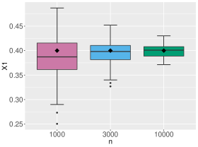
(a) coefficients for $x_{1}$ of $\mu_{1}$

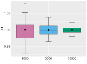
(b) coefficients for $x_{1}$ of $\mu_{2}$

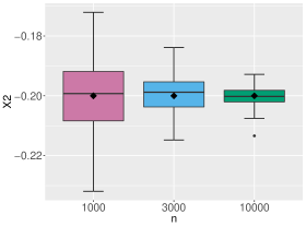
(c) coefficients for $x_{2}$ of $\mu_{2}$

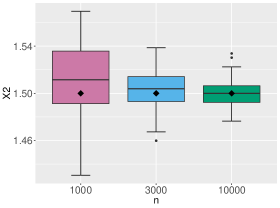
(d) coefficients for $x_{3}$ of $\sigma_{2}$

Figure 8: Simulation results for linear effects in scenario 1. The boxplots represent the estimated linear coefficients in $N=100$ iterations. The true values of the coefficients are denoted by the black diamond symbols.

Figure 9 exemplarily shows the estimated smooth functions against the true ones for scenario 1 and $n=1,000$. The procedure is able to recover the smooth functions satisfactorily although some of the curves are wigglier or too smooth compared to the true functions. This effect vanishes in the other cases as the sample size grows. Note that for the location parameter of the continuous marginal, the smooth effects seem to be easier to estimate as all curves are very close to the true functions. If we increase the sample size, the fit of the smooth functions improves significantly especially at the local minima and maxima (plots are available upon request).

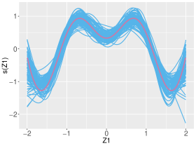
(a) $s_{1}^{\mu_{1}}(\nu_{1})$

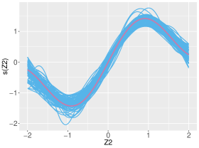
(b) $s_{2}^{\mu_{1}}(\nu_{2})$

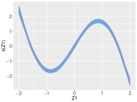
(c) $s_{3}^{\mu_{2}}(\nu_{1})$

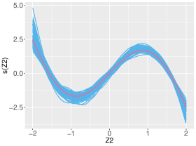
(d) $s_{3}^{\gamma}(\nu_{2})$

Figure 9: Simulation results for non-linear effects in scenario 1. The pink solid lines represent the true functions.

Note that some simulation iterations for the case of $n=1,000$ were problematic in that the smooth functions were not estimated adequately. Their number was rather small and we excluded them. Table 5 gives an overview of how many iterations were excluded.

The results for scenarios 2, 3 and 4 are similar to the first one and shown in Figures 10, 11 and 12, respectively. Again, the estimation of the smooth terms improves considerably as the sample size increases but we only show the more difficult case of $n=1,000$ here to demonstrate that results are still acceptable also at relatively small sample sizes.

scenario	case	rejected by algorithm	manually deleted
scenario 1	n = 1,000	0	3
	n = 3,000	0	0
	n = 10,000	0	0
scenario 2	n = 1,000	1	1
	n = 3,000	1	0
	n = 10,000	1	0
scenario 3 (J0)	n = 1,000	62	2
	n = 3,000	3	0
	n = 10,000	0	0
scenario 4	n = 1,000	77	1
	n = 3,000	3	0
	n = 10,000	2	0

Table 5: Number of repeated iterations due to warning messages and number of manually deleted iterations that were extreme outliers.

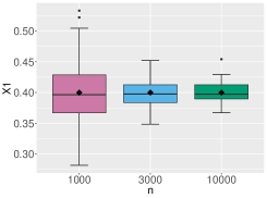
(a) coefficients for $x_{1}$ of $\mu_{1}$

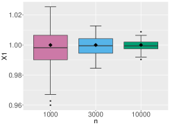
(b) coefficients for $x_{1}$ of $\mu_{2}$

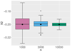
(c) coefficients for $x_{2}$ of $\mu_{2}$

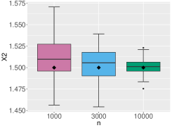
(d) coefficients for $x_{3}$ of $\sigma_{2}$

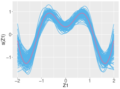
(e) $s_{1}^{\mu_{1}}(\nu_{1})$

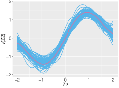
(f) $s_{2}^{\mu_{1}}(\nu_{2})$

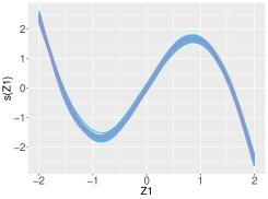
(g) $s_{3}^{\mu_{2}}(\nu_{1})$

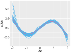
(h) $s_{3}^{\gamma}(\nu_{2})$

Figure 10: Simulation results for linear and non-linear effects (case $n=1000$) in scenario 2. The boxplots represent the estimated linear coefficients in $N=100$ iterations. The true values of the coefficients are denoted by the black diamond symbols. The pink solid lines represent the true functions of the non-linear effects.

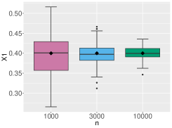
(a) coefficients for $x_{1}$ of $\mu_{1}$

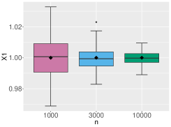
(b) coefficients for $x_{1}$ of $\mu_{2}$

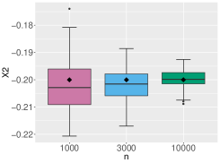
(c) coefficients for $x_{2}$ of $\mu_{2}$

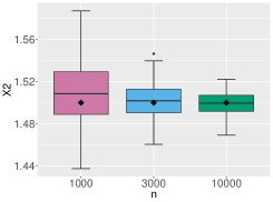
(d) coefficients for $x_{3}$ of $\sigma_{2}$

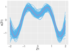
(e) $s_{1}^{\mu_{1}}(\nu_{1})$

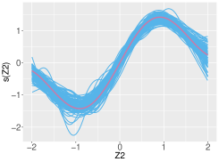
(f) $s_{2}^{\mu_{1}}(\nu_{2})$

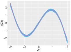
(g) $s_{3}^{\mu_{2}}(\nu_{1})$

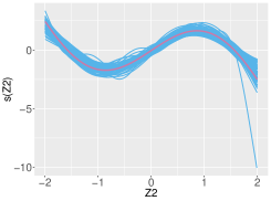
(h) $s_{3}^{\gamma}(\nu_{2})$

Figure 11: Simulation results for linear and non-linear effects (case $n=1000$) in scenario 3. The boxplots represent the estimated linear coefficients in $N=100$ iterations. The true values of the coefficients are denoted by the black diamond symbols. The pink solid lines represent the true functions of the non-linear effects.

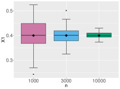
(a) coefficients for $x_{1}$ of $\mu_{1}$

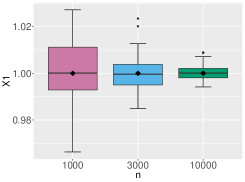
(b) coefficients for $x_{1}$ of $\mu_{2}$

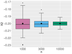
(c) coefficients for $x_{2}$ of $\mu_{2}$

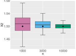
(d) coefficients for $x_{3}$ of $\sigma_{2}$

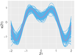
(e) $s_{1}^{\mu_{1}}(\nu_{1})$

(f) $s_{2}^{\mu_{1}}(\nu_{2})$

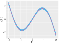
(g) $s_{3}^{\mu_{2}}(\nu_{1})$

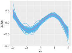
(h) $s_{3}^{\gamma}(\nu_{2})$

Figure 12: Simulation results for linear and non-linear effects (case $n=1000$) in scenario 4. The boxplots represent the estimated linear coefficients in $N=100$ iterations. The true values of the coefficients are denoted by the black diamond symbols. The pink solid lines represent the true functions of the non-linear effects.

Appendix F Additional material for the application case

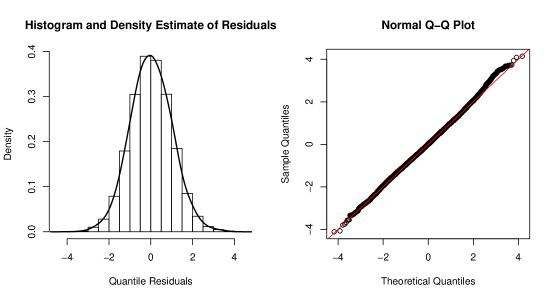
Figure 13: Histogram and normal Q-Q plots for the log-normal continuous margin of the final bivariate copula model.

Table 6: Effects on education

	Estimate	Std. Error	z value	Pr($>$$|$z$|$)
cutoff 1	-3.170	0.071	-44.348	0.000
cutoff 2	-0.201	0.008	-24.059	0.000
cutoff 3	0.761	0.006	129.930	0.000
cutoff 4	2.618	0.006	413.481	0.000
marital status of household head: married	-0.460	0.063	-7.272	0.000
marital status of household head: separated	-0.637	0.089	-7.128	0.000
marital status of household head: widowed	-0.448	0.073	-6.151	0.000
household head is male	0.185	0.042	4.353	0.000
urban dummy	1.042	0.022	48.383	0.000
number of children: 1	-0.166	0.028	-5.969	0.000
number of children: 2	-0.131	0.030	-4.366	0.000
number of children: 3	-0.168	0.043	-3.936	0.000
number of children: 4-7	-0.332	0.067	-4.949	0.000
number of elderly: 1	-0.003	0.031	-0.111	0.912
number of elderly: 2 or 3	0.191	0.059	3.250	0.001
religion: Christian	1.002	0.047	21.175	0.000
religion: Hinduism and other	-0.028	0.048	-0.576	0.565
Note: Base categories for marital status is “not yet married”, for number of children “no children”, for number of elderly “no elderly”, and for religion “Islam”.

Table 7: Effects on $\mu$ of the income distribution

	Estimate	Std. Error	z value	Pr($>$$|$z$|$)
Intercept	14.430	0.031	465.128	0.0000
marital status of household head: married	-0.142	0.021	-6.674	0.0000
marital status of household head: separated	-0.140	0.029	-4.834	0.0000
marital status of household head: widowed	-0.145	0.024	-5.997	0.0000
household head is male	-0.060	0.013	-4.754	0.0000
education of household head: primary	0.127	0.022	5.734	0.0000
education of household head: middle school	0.245	0.023	10.713	0.0000
education of household head: high school	0.388	0.023	16.944	0.0000
education of household head: tertiary education	0.663	0.026	25.048	0.0000
urban dummy	0.120	0.007	17.852	0.0000
number of children: 1	-0.259	0.008	-32.190	0.0000
number of children: 2	-0.414	0.009	-47.637	0.0000
number of children: 3	-0.559	0.012	-45.353	0.0000
number of children: 4-7	-0.738	0.019	-39.319	0.0000
number of elderly: 1	-0.189	0.009	-21.082	0.0000
number of elderly: 2 or 3	-0.312	0.017	-18.660	0.0000
religion: Christian	0.059	0.016	3.818	0.0001
religion: Hinduism and other	0.166	0.026	6.441	0.0000
Note: Base categories for marital status is “not yet married”, for education “no schooling”, for number of children “no children”, for number of elderly “no elderly”, and for religion “Islam”.

Table 8: Effects on $\sigma$ of the income distribution

	Estimate	Std. Error	z value	Pr($>$$|$z$|$)
Intercept	-0.426	0.022	-19.394	0.000
marital status of household head: married	-0.176	0.023	-7.617	0.000
marital status of household head: separated	-0.075	0.033	-2.262	0.024
marital status of household head: widowed	-0.116	0.026	-4.458	0.000
number of children: 1	-0.065	0.011	-6.132	0.000
number of children: 2	-0.081	0.011	-7.021	0.000
number of children: 3	-0.066	0.017	-4.000	0.000
number of children: 4-7	-0.076	0.026	-2.958	0.003
religion: Christian	0.046	0.019	2.394	0.017
religion: Hinduism and other	0.035	0.026	1.310	0.190
Note: Base categories for marital status is “not yet married”, for number of children “no children”, for number of elderly “no elderly”, and for religion “Islam”.

Table 9: Effects on the copula parameter

	Estimate	Std. Error	z value	Pr($>$$|$z$|$)
Intercept	-0.179	0.045	-3.998	0.000
marital status of household head: married	0.143	0.034	4.219	0.000
marital status of household head: separated	0.170	0.048	3.517	0.000
marital status of household head: widowed	0.177	0.039	4.543	0.000
education of household head: primary	0.061	0.033	1.877	0.060
education of household head: middle school	0.104	0.036	2.906	0.004
education of household head: high school	0.161	0.033	4.853	0.000
education of household head: tertiary education	0.120	0.036	3.337	0.001
urban dummy	0.101	0.013	7.816	0.000
number of children: 1	0.018	0.016	1.128	0.259
number of children: 2	0.041	0.017	2.411	0.016
number of children: 3	0.084	0.025	3.391	0.001
number of children: 4-7	0.063	0.036	1.746	0.081
number of elderly: 1	0.075	0.017	4.402	0.000
number of elderly: 2 or 3	0.113	0.030	3.748	0.000
Note: Base categories for marital status is “not yet married”, for education “no schooling”, for number of children “no children”, and for number of elderly “no elderly”.

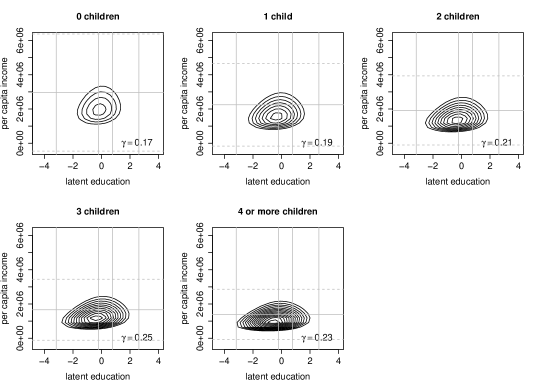
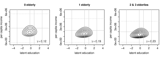
Figure 14: Contour plots for (education, income)’ and a Gaussian copula by different numbers of children and elderly living in the same household. Contour lines of densities are at levels from 0.00000005 to 0.00000025 in 0.00000001 steps. The vertical straight lines represents the cut off values for the education categories, horizontal straight lines are the consumption average, and dashed horizontal line are at two standard deviations around this average.

Appendix G Software

We incorporated the models proposed this paper into the GJRM package (Marra and Radice, 2019) in R (R Core Team, 2019). A mixed ordered-continuous model is called by setting the option ordinal = TRUE. The main fitting function, gjrm(), is very easy to use in that its syntax follows those of linear models, generalized linear models, or generalized additive models. The function CopulaCLM() is called internally to fit this specific model. An example of model specification is given below.

eq.educ <- educ_att ~ s(age) + as.factor(hhmarstat) + as.factor(hhmale) +
                      as.factor(urban) + as.factor(num_child) +
                      as.factor(elderly) + as.factor(relig)

eq.mu   <- pce.defl ~ s(age) + as.factor(hhmarstat) + as.factor(hhmale) +
                      as.factor(urban) + as.factor(num_child) +
                      as.factor(elderly) + as.factor(relig) +
                      as.factor(hheduc) + s(prov, bs = "mrf", xt = xt1, k = 15)

eq.si   <-          ~ s(age) + as.factor(hhmarstat) +
                      as.factor(num_child) + as.factor(elderly) +
                      as.factor(relig) + s(prov, bs = "mrf", xt = xt1, k = 15)

eq.theta <-         ~ s(age) + as.factor(hhmarstat) +
                      as.factor(urban) + as.factor(num_child) +
                      as.factor(elderly) + as.factor(hheduc) +
                      s(prov, bs = "mrf", xt = xt1, k = 15)

form.list <- list(eq.educ, eq.mu, eq.si, eq.theta)

mod.edu <- gjrm(form.list, data = na.omit(df), ordinal = TRUE,
                     Model = "B", BivD = "N", margins = c("logit", "LN"),
                     drop.unused.levels = FALSE, gamlssfit = TRUE)

Te user first specifies the four equations for the model’s parameters of the marginal distributions and of the copula, which are stored in the list form.list. Continuous variables enter the model specifications via smooth effects s() represented (by default) via thin-plate regression splines (argument bs = "tp") with ten basis function and second order derivative penalties. Spatial effects of the provinces are modeled using Markov random fields with neighbourhood structure xt1 and 15 knots (argument bs = "mrf"). Argument Model = "B" specifies that a bivariate model will be estimated, margins = c("logit", "LN") gives the marginal distributions and BivD = "N" specifies the Gaussian copula. The argument ordinal must be set to TRUE in order to fit a mixed ordered-continuous model and the ordinal outcome educ_att must be numeric. The optional argument gamlssfit = TRUE uses starting values obtained from a univariate gamlss and drop.unused.levels = FALSE is needed because not all of the provinces specified via the Markov random fields have observations in the data frame df. Functions summary(), plot(), AIC() and BIC() can employed in the usual manner. It is advisable to use post.check() after fitting the model to produce plots of normalized quantile residuals. More details, options, and the available choices for the marginal distributions and copula functions can be found in the documentation of the GJRM package.

References

- (1)
- Akita (2017) Akita, T.: 2017, Educational expansion and the role of education in expenditure inequality in indonesia since the 1997 financial crisis, Social Indicators Research 130(3), 1165–1186.
- Alkire et al. (2012) Alkire, S., Conconi, A. and Roche, J. M.: 2012, Multidimensional poverty index 2012: Brief methodological note and results, University of Oxford, Department of International Development, Oxford Poverty and Human Development Initiative, Oxford, UK .
- Alkire and Fang (2018) Alkire, S. and Fang, Y.: 2018, Dynamics of multidimensional poverty and uni-dimensional income poverty: An evidence of stability analysis from china, Social Indicators Research .
- Alkire et al. (2004) Alkire, S., Foster, J. E., Seth, S., Santos, M. E., Roche, J. M. and Ballon, P. (eds): 2004, Multidimensional Poverty Measurement and Analysis, Oxford University Press, Oxford.
- Barham et al. (1995) Barham, V., Boadway, R., Marchand, M. and Pestieau, P.: 1995, Education and the poverty trap, European Economic Review 39(7), 1257 – 1275.
- Belitz et al. (2015) Belitz, C., Brezger, A., Klein, N., Kneib, T., Lang, S. and Umlauf, N.: 2015, BayesX - Software for Bayesian Inference in Structured Additive Regression Models. Version 3.0.2. Available from http://www.bayesx.org.
- Bhattacharyya and Resosudarmo (2015) Bhattacharyya, S. and Resosudarmo, B. P.: 2015, Growth, growth accelerations, and the poor: Lessons from indonesia, World Development 66, 154 – 165.
- Calvo and Dercon (2013) Calvo, C. and Dercon, S.: 2013, Vulnerability to individual and aggregate poverty, Social Choice and Welfare 41(4), 721–740.
- Decancq (2014) Decancq, K.: 2014, Copula-based measurement of dependence between dimensions of well-being, Oxford Economic Papers 66(3), 681–701.
- Donat and Marra (2017) Donat, F. and Marra, G.: 2017, Semi-parametric bivariate polychotomous ordinal regression, Statistics and Computing 27(1), 283–299.
- Donat and Marra (2018) Donat, F. and Marra, G.: 2018, Simultaneous equation penalized likelihood estimation of vehicle accident injury severity, Journal of the Royal Statistical Society: Series C (Applied Statistics) 67(4), 979–1001.
- Duclos et al. (2006) Duclos, J.-Y., Sahn, D. E. and Younger, S. D.: 2006, Robust multidimensional poverty comparisons, The Economic Journal 116(514), 943–968.
- Duflo (2004) Duflo, E.: 2004, The medium run effects of educational expansion: evidence from a large school construction program in indonesia, Journal of Development Economics 74(1), 163 – 197.
-
Geyer (2015)
Geyer, C. J.: 2015, trust: Trust Region Optimization.
R package version 0.1-7.
https://CRAN.R-project.org/package=trust - Günther and Harttgen (2009) Günther, I. and Harttgen, K.: 2009, Estimating Households Vulnerability to Idiosyncratic and Covariate Shocks: A Novel Method Applied in Madagascar, World Development 37(7), 1222–1234.
- Haberman (1980) Haberman, S. J.: 1980, Discussion of "Regression models for ordinal data" by Peter McCullagh, Journal of the Royal Statistical Society: Series B (Statistical Methodology) 42(2), 136–137.
- Hohberg and Lay (2015) Hohberg, M. and Lay, J.: 2015, The impact of minimum wages on informal and formal labor market outcomes: evidence from indonesia, IZA Journal of Labor & Development 4(1), 14.
- Kalliovirta (2008) Kalliovirta, L.: 2008, Quantile residuals for multivariate models, Technical Report 247, Helsinki Center of Economic Research.
- Kauermann (2005) Kauermann, G.: 2005, Penalized spline smoothing in multivariable survival models with varying coefficients, Computational Statistics & Data Analysis 49(1), 169 – 186.
- Kauermann et al. (2009) Kauermann, G., Krivobokova, T. and Fahrmeir, L.: 2009, Some asymptotic results on generalized penalized spline smoothing, Journal of the Royal Statistical Society: Series B (Statistical Methodology) 71(2), 487–503.
- Kleiber and Kotz (2003) Kleiber, C. and Kotz, S.: 2003, Statistical Size Distributions in Economics and Actuarial Sciences, Wiley, Hoboken.
- Klein and Kneib (2016) Klein, N. and Kneib, T.: 2016, Simultaneous inference in structured additive conditional copula regression models: a unifying bayesian approach, Statistics and Computing 26(4), 841–860.
- Klein et al. (2015) Klein, N., Kneib, T., Klasen, S. and Lang, S.: 2015, Bayesian structured additive distributional regression for multivariate responses, Journal of the Royal Statistical Society: Series C (Applied Statistics) 64(4), 569–591.
- Klein et al. (2019) Klein, N., Kneib, T., Marra, G., Radice, R., Rokicki, S. and McGovern, M. E.: 2019, Mixed Binary-Continuous Copula Regression Models with Application to Adverse Birth Outcomes, Statistics in Medicine 38(3), 413–436.
- Kobus and Kurek (2018) Kobus, M. and Kurek, R.: 2018, Copula-based measurement of interdependence for discrete distributions, Journal of Mathematical Economics 79, 27 – 39.
- Marra and Radice (2017) Marra, G. and Radice, R.: 2017, Bivariate copula additive models for location, scale and shape, Computational Statistics & Data Analysis 112, 99–113.
-
Marra and Radice (2019)
Marra, G. and Radice, R.: 2019, GJRM: Generalised Joint Regression
Modelling.
R package version 0.2.
https://CRAN.R-project.org/package=GJRM - Marra et al. (2017) Marra, G., Radice, R., Bärnighausen, T., Wood, S. N. and McGovern, M. E.: 2017, A simultaneous equation approach to estimating HIV prevalence with nonignorable missing responses, Journal of the American Statistical Association 112(518), 484–496.
- Marra and Wood (2012) Marra, G. and Wood, S. N.: 2012, Coverage properties of confidence intervals for generalized additive model components, Scandinavian Journal of Statistics 39(1), 53–74.
- McKelvey and Zavoina (1975) McKelvey, R. D. and Zavoina, W.: 1975, A statistical model for the analysis of ordinal level dependent variables, The Journal of Mathematical Sociology 4(1), 103–120.
- Nelsen (2006) Nelsen, R.: 2006, An Introduction to Copulas, Springer, New York.
- Nocedal and Wright (2006) Nocedal, J. and Wright, S. J.: 2006, Numerical Optimization, second edn, Springer, New York, NY, USA.
- Perez and Prieto (2015) Perez, A. and Prieto, M.: 2015, Measuring dependence between dimensions of poverty in Spain: An approach based on copulas, Proceedings of the Conference of the International Fuzzy Systems Association and the European Society for Fuzzy Logic and Technology (IFSA-EUSFLAT-15), pp. 734–741.
- Quinn (2007) Quinn, C.: 2007, Using copulas to measure association between ordinal measures of health and income, Technical Report 07/24, University of York.
-
R Core Team (2019)
R Core Team: 2019, R: A Language and Environment for Statistical
Computing, R Foundation for Statistical Computing, Vienna, Austria.
https://www.R-project.org/ - Radice et al. (2016) Radice, R., Marra, G. and Wojtyś, M.: 2016, Copula regression spline models for binary outcomes, Statistics and Computing 26(5), 981–995.
-
RAND (2017)
RAND: 2017, The Indonesia Family Life Survey (IFLS).
https://www.rand.org/labor/FLS/IFLS.html - Rigby and Stasinopoulos (2005) Rigby, R. A. and Stasinopoulos, D. M.: 2005, Generalized Additive Models for Location, Scale and Shape, Journal of the Royal Statistical Society: Series C (Applied Statistics) 54(3), 507–554.
- Rue and Held (2005) Rue, H. and Held, L.: 2005, Gaussian Markov Random Fields: Theory and Applications, Chapman & Hall, London.
- Ruppert et al. (2003) Ruppert, D., Wand, M. P. and Carroll, R. J.: 2003, Semiparametric Regression, Cambridge Series in Statistical and Probabilistic Mathematics, Cambridge University Press, Cambridge.
- Sklar (1959) Sklar, A.: 1959, Fonctions de reepartition a n dimensions et leurs marges, Publications de l’Institut de Statistique de l’Universite de Paris 8, 229–231.
- Strauss et al. (2016) Strauss, J., Witoelar, F. and Sikoki, B.: 2016, The Fifth Wave of the Indonesia Family Life Survey: Overview and Field Report, Volume 1.
- Tan et al. (2018) Tan, B. K., Panagiotelis, A. and Athanasopoulos, G.: 2018, Bayesian inference for the one-factor copula model, Journal of Computational and Graphical Statistics (to appear) .
- Thi Nguyen et al. (2015) Thi Nguyen, K. A., Jolly, C. M., Bui, C. T. P. N. and Le, T. H. T.: 2015, Climate change, rural household food consumption and vulnerability: The case of Ben Tre province in Vietnam, Agricultural Economics Review 16(2), 95–109.
- Wahba (1978) Wahba, G.: 1978, Improper priors, spline smoothing and the problem of guarding against model errors in regression, Journal of the Royal Statistical Society. Series B (Methodological) 40(3), 364–372.
- Wood (2015) Wood, S.: 2015, Core Statistics, Institute of Mathematical Statistics, Cambridge University Press, New York, NY.
- Wood (2017) Wood, S.: 2017, Generalized Additive Models: An Introduction with R, Second Edition, Chapman & Hall/CRC Texts in Statistical Science, CRC Press, Boca Raton, FL.
- Wood (2004) Wood, S. N.: 2004, Stable and efficient multiple smoothing parameter estimation for generalized additive models, Journal of the American Statistical Association 99(467), 673–686.
- Wood (2006) Wood, S. N.: 2006, On confidence intervals for generalized additive models based on penalized regression splines, Australian & New Zealand Journal of Statistics 48(4), 445–464.
- World Bank (2018) World Bank: 2018, Piecing together the poverty puzzle, Technical report, World Bank, Washington, DC.
- Zereyesus et al. (2017) Zereyesus, Y. A., Embaye, W. T., Tsiboe, F. and Amanor-Boadu, V.: 2017, Implications of non-farm work to vulnerability to food poverty-recent evidence from northern Ghana, World Development 91, 113–124.