From Reflecting Brownian Motion to Reflected Stochastic Differential Equations: A Systematic Survey and Complementary Study

Abstract

This work contributes a systematic survey and complementary insights of reflecting Brownian motion and its properties. Extension of the Skorohod problem’s solution to more general cases is investigated, based on which a discussion is further conducted on the existence of solutions for a few particular kinds of stochastic differential equations with a reflected boundary. It is proved that the multidimensional version of the Skorohod equation can be solved under the assumption of a convex domain (D).

1 Introduction

Brownian motion and reflecting Brownian motion have a set of properties that hold great potential for game-changing applications, ranging from the mathematical study of queuing models with heavy traffic (Reiman (1984)), to statistical physics (Lang (1995)), and the recent advances in statistical mechanics (Grebenkov (2019)). Underpinned by the It$\hat{o}$’s calculus (Malliaris (1983)), the Brownian motion inspired models arguably lay a foundation for quantitative finance, as evidenced notably in the stock market forecasting (Guo and Li (2019)), the valuations of options based on the Black–Scholes–

Merton model (Calin (2012)) in lattice-based computation or Monte Carlo based derivative investment instruments (Zhang (2020)) with multiple sources of uncertainty.

Fundamentally, the reflecting Brownian motion can be characterised by the Skorohod problem into solving a stochastic differential equation (SDE) with a reflecting boundary condition. Over decades, there has been a continuous research campaign to attempt solutions of the Skorohod stochastic differential equation with reflecting (Saisho (1987)), semi-reflecting (Kanagawa (2009)), or absorption (Berestycki et al. (2014)) boundary conditions. By way of illustration, (D’Auria and Kella (2012)) reports a reflected Markov-modulated Brownian motion with a two-sided reflection, which generalises the reflected Brownian motion to the Markov modulated case. More recently, Monte Carlo simulation was employed by (Malsagov and Mandjes (2019)) for closed-form approximations of the mean and variance of fractional Brownian motion reflected at level 0, the problem of which explicit expressions and numerical methods struggle to address. Apart from the discretization error reported by (Asmussen et al. (1995)), there remain massive technological gaps that challenge the conventional statistical thinking in tailoring the reflecting Brownian motion and its properties for real-life emerging applications, such as the contact tracing (Li and Guo (2020)) for the coronavirus disease (COVID-19), the statistical clutter modelling and phased array signal processing for 5G communications (Li (2020)) and beyond.

This paper is organised into the following sections. First, the elements of Brownian Motion and the stochastic integral are elaborated in sections 2 and 3, respectively. Section 4 presents the survey and insights into the reflecting Brownian motion, followed by the in-depth discussion of reflected stochastic differential equations in section 5.

2 Brownian Motion

In this section, we will introduce the definition of Brownian motion and reflecting brownian motion, which are the most important stochastic process that is widely used in applications.

2.1 Brownian motion

Definition 2.1.1(Brownian Motion): A stochastic process X=($X_{t}$,t$\geq$0) is called a d-dimensional Brownian motion(or Wiener process) with the initial probability law $\mu$, if

(i) $X_{t}$ is continuous in t almost surely and $X_{0}$ has the distribution law $\mu$ on $\mathbb{R}^{d}$;

(ii) $X_{t}$ has independent increments, that is for any 0$\leq t_{0}<t_{1}<...<t_{n}$, the random variables,

$X_{t_{n}}-X_{t_{n-1}},X_{t_{n-1}}-X_{t_{n-2}},...,X_{t_{2}}-X_{t_{1}}$

are independent with each other;

(iii) for all 0$\leq s<t$,

$X_{t}-X_{s}\sim$N(0,t-s)

Then, for every 0$<t_{1}<...<t_{m}$ and $A_{i}\in\mathcal{B}(\mathbb{R}^{d})$, i=1,2,…,m, we have the probability as

P($X_{t_{1}}\in A_{1},X_{t_{2}}\in A_{2},...,A_{t_{m}}\in A_{m}$)

=$\int_{\mathbb{R}^{d}}\mu(dx)\int_{A_{1}}p(t_{1},x_{1}-x)dx_{1}\int_{A_{2}}p(t_{2}-t_{1},x_{2}-x_{1})dx_{2}$

…$\int_{A_{m}}p(t_{m}-t_{m-1},x_{m}-x_{m-1})dx_{m}$

where, p(t,x),$t>0$, x$\in\mathbb{R}^{d}$, is defined by

p(t,x)=(2$\pi t)^{-d/2}exp[-|x|^{2}/2t]$,

being the probability distribution function of a d-dimensional Gaussian distribution.

Then we are going to introduce a new concept called Brownian local time which will be used in the upcoming proof.

Let X=($X_{t}$) be a one-dimensional Brownian motion defined on the probability space ($\Omega$,F,P).

*Definition 2.1.2(Brownian local time)Ikeda and Watanabe (2014):By the local time or the sojourn time density of X we mean family of non-negative random variables $\phi(t,x,\omega),t\in[0,\infty),x\in R^{1}$ such that, with probability one, the following holds:

(i) (t,x) $\mapsto\phi$(t,s) is continuous,

(ii) for every Borel subset A of $R^{1}$ and t$\geq$0

$\int^{t}_{0}I_{A}(X_{s})ds$=2$\int_{A}\phi(t,s)dx$.

It is clear that if such a family {$\phi$(t,x)} exists, then it is unique and is given by

$\phi(t,x)=lim_{\epsilon\downarrow 0}\frac{1}{4\epsilon}\int^{t}_{0}I_{(x-\epsilon,x+\epsilon)}(X_{s})ds$.

2.2 Skorohod problem and Skorohod equation

Before moving on to reflecting Brownian motion, we will introduce a concept called Skorohod problem. It is useful when characterising the reflecting Brownian motion.

In probability theory, the Skorokhod problem is the problem of solving a stochastic differential equation with a reflecting boundary condition. Let us firstly see the one dimensional version.

We set $W_{0}^{1}$ = {f$\in$$\mathbb{C}$([0,$\infty)$$\longrightarrow$$\mathbb{R}$); f(0)=0} and $C^{+}$ = {f$\in\mathbb{C}([0,\infty$)$\longrightarrow$$\mathbb{R}$); f(t)$\geq$0 for all t$\geq$0}.

Lemma 2.2.1 Ikeda and Watanabe (2014): Given f$\in$$W_{0}^{1}$ and x$\in$$\mathbb{R}^{+}$, there exist unique g$\in$$C^{+}$ and h$\in$$C^{+}$ such that

(i) g(t)=x+f(t)+h(t),

(ii)h(0)=0 and t$\mapsto$h(t) is increasing,

(iii) $\int^{t}_{0}$$I_{0}$(g(s))dh(s)=h(t), i.e., h(t) increases only on the set of t when g(t)=0.

Proof:

Set

g(t)=x+f(t)-$min_{0\leq s\leq t}${(x+f(s))$\land$0},

h(t)=-$min_{0\leq s\leq t}${(x+f(s))$\land$0}.

Then we will prove that g(t) and h(t) satisfy the above conditions (i), (ii) and (iii). According to the definition of g(t) and h(t), (i) apparently holds. So we only need to check (ii) and (iii).

For (ii), h(0)=-{(x+f(0)$\land$0}.

For (ii), h(0)=-{(x+f(0)$\land$0}.

x>0 and f(0)=0 since x $\in R^{+}$, f $\in W_{0}^{\prime}$ $\implies$ x+f(0)>0

So h(0) = -0 = 0.

Assume $t_{1}<t_{2}$, $t_{1},t_{2}\in[0,\infty)$. Then $min_{0\leq s\leq t_{1}}${(x+f(s)) $\land$0} $\leq$ $min_{0\leq s\leq t_{2}}${(x+f(s)) $\land$0} because [0, $t_{1}$] $\subseteq$ [0, $t_{2}$]. So h($t_{1}$)=$min_{0\leq s\leq t_{1}}${(x+f(s)) $\land$0} $\leq$ $min_{0\leq s\leq t_{2}}${(x+f(s)) $\land$0}=h($t_{2}$), i.e. t $\mapsto$h(t) is increasing.

Hence (ii) holds.

To prove (iii), we need to prove that the set I, which is the union of the intervals on which h(t) increases, is included by $I_{0}$(g(t)).

Assume that, $min_{0\leq s\leq t}${x+f(s)} decreases on interval I’, i.e. $min_{0\leq s\leq b}${x+f(s)} $\leq$$min_{0\leq s\leq a}${x+f(s)} for all b>a, where a,b $\in$I’. When b$\longrightarrow$a,

-(x+f(b))=-$min_{0\leq s\leq b}${x+f(s)}=h(b),

and

-$min_{0\leq s\leq a}${x+f(s)}=h(a)= $lim_{b\longrightarrow a}$h(b)= $lim_{b\longrightarrow a}$-(x+f(b))=-(x+f(a)),

since h(t) and f(t) are both continuous.

Therefore, g(a)=0, g(b)=0. Then because a,b $\in$I’ are arbitrary, g(t)=0 on I’, i.e. I $\subseteq I_{0}(g(t))$. Hence (iii) holds.

We shall prove the uniqueness. Suppose $g_{1}$(t) and $h_{1}$(t) $\in C_{+}$ also satisfy the condition (i), (ii) and (iii). Then

g(t)- $g_{1}$(t)=h(t)- $h_{1}$(t) for all t $\geq$0.

If there exists $t_{1}>$0 such that g($t_{1}$)-$g_{1}(t_{1})>$0, we set $t_{2}$= max{ t$<t_{1}$; g(t)-$g_{1}$(t)=0}. Then g(t)$>g_{1}$(t)$\geq$0 for all t $\in(t_{2},t_{1}]$ and hence, by (iii), h($t_{1}$)-h($t_{2}$)=0. Since $h_{1}$(t) is increasing, we have

0$<g(t_{1}$)-$g_{1}(t_{1})$=h($t_{1}$)-$h_{1}(t_{1})\leq$h($t_{2}$)-$h_{1}(t_{2})$=g($t_{2}$)-$g_{1}(t_{2})$=0.

This is contradiction. Therefore g(t)$\leq g_{1}$(t) for all t $\geq$0. By symmetry, g(t)$\geq g_{1}$(t) for all t $\geq$0. Hence g(t)$\equiv g_{1}$(t) and so h(t)$\equiv h_{1}$(t).

2.3 Reflecting Brownian motion

From the name, we can easily see that this Brownian motion has bounds and gets reflected when it goes beyond the bounds.

Definition 2.3.1(Reflecting Brownian motion) Ikeda and Watanabe (2014): Let X=($X_{t}$) be a one-dimensional Brownian motion and let $X^{+}$=($X^{+}_{t}$) be a continuous stochastic process on [0,$\infty$) defined by

$X^{+}_{t}=|X_{t}|$.

Then we can easily infer that the event {$X^{+}_{t_{2}}=y|X_{t_{1}}=x$} is the union of {$X_{t_{2}}=y|X_{t_{1}}=x$} and {$X_{t_{2}}=-y|X_{t_{1}}=x$}, i.e.

{$X^{+}_{t_{2}}=y|X_{t_{1}}=x$}={$X_{t_{2}}=y|X_{t_{1}}=x$}$\cup${$X_{t_{2}}=-y|X_{t_{1}}=x$}

={$X_{t_{2}-t_{1}}=y-x$}$\cup${$X_{t_{2}-t_{1}}=-y-x$}.

What’s more, since $X_{t-s}\sim$N(0,t-s), we have that for 0$<t_{1}<t_{2}<...<t_{n}$, $A_{t}\in\mathcal{B}([0,\infty$)),

P[$X^{+}_{t_{1}}\in A_{1}$,$X^{+}_{t_{2}}\in A_{2}$,…,$X^{+}_{t_{n}}\in A_{n}$]

=$\int_{[0,\infty)}\mu(dx)\int_{A_{1}}p^{+}(t_{1},x,x_{1})dx_{1}\int_{A_{2}}p^{+}(t_{2}-t_{1},x_{1},x_{2})dx_{2}$

…$\int_{A_{1}}p^{+}(t_{n}-t_{n-1},x_{n-1},x_{n})dx_{n}$

where

$p^{+}(t,x,y)=\frac{1}{\sqrt{2\pi t}}(exp[-\frac{(x-y)^{2}}{2t}]+exp[-\frac{(x+y)^{2}}{2t}])$

and $\mu^{+}$ is the probability law of $X_{0}^{+}=|X^{+}_{0}|$. The process $X^{+}$ is called the one-dimensional reflecting Brownian motion. An illustrated one-dimensional Brownian motion and the associated reflected path are plotted in Figure 1.

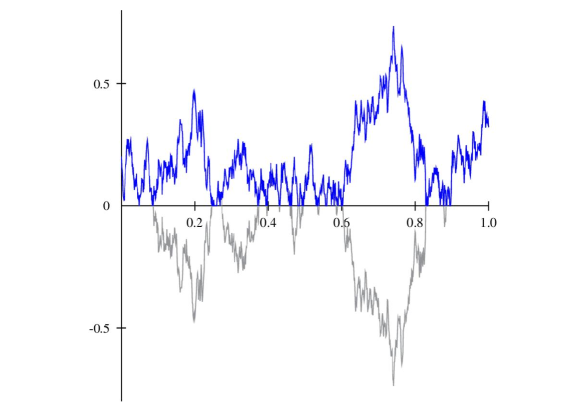
Figure 1: A path of a Brownian motion (grey) and the associated reflected path (blue)

There are different ways to characterise reflecting Brownian motion. We will present a characterisation due to Skorohod problem.

Theorem 2.3.2 Ikeda and Watanabe (2014): Let {X(t), B(t),$\phi$(t)} be a system of real continuous stochastic processes defined on a probability space such that B(t) is a one-dimensional Brownian motion with B(0)=0, X(0) and process B(t) are independent and with probability one the following holds:

(i) X(t)$\geq$0 for all t $\geq$0 and $\phi$(t) is increasing with $\phi$(0)=0 such that

$\int_{0}^{t}I_{0}$(X(s))d $\phi$(s) = $\phi$(t);

(ii)

$$X(t)=X(0)+B(t)+\phi(t).$$ (1)

Then X=X(t) is a reflecting Brownian motion on [0,$\infty$).

Equation (2.1) is called the Skorohod equation which will be introduced in the next section.

Proof: By Lemma 2.2.1, X = X(t) and $\phi=\phi$(t) are uniquely determined by X(0) and B = B(t): X = X(0)+B(t)-$min_{0\leq s\leq t}${(X(0)+B(s))$\land$0} and $\phi$= -$min_{0\leq s\leq t}${(X(0)+B(s))$\land$0}. To prove this theorem we only need to show that if $x_{t}$ is a one-dimensional Brownian motion, then X(t) = $|x_{t}|$ satisfies, with some processes B(t) and $\phi$(t), the above properties. Let $g_{n}$(x) be a non-negative continuous function on $R^{1}$ with support in (0,1/n), i.e. supp($g_{n}$)={x $\in[0,\infty)|g_{n}$(t)$\neq$0}=(0,1/n), such that $\int_{0}^{\infty}g_{n}$(x)dx=1. Set

$u_{n}$(x) = $\int_{0}^{|x|}$dy $\int_{0}^{y}g_{n}$(z)dz.

Then we can see that $u_{n}\in C^{2}$(R), $u_{n}$’(x) =$\frac{d|x|}{dx}\int_{0}^{|x|}g_{n}(z)dz$. And then $|u_{n}^{\prime}|$ $\leq|\frac{d|x|}{dx}||\int_{0}^{\infty}g_{n}(z)dz|\leq$1, $u_{n}$(0)=0, $u_{n}$(x) $\uparrow|x|$. Then because $lim_{n\longrightarrow\infty}\frac{1}{n}$=0 and non-negative function $g_{n}$ has support in (0,1/n),

$lim_{n\longrightarrow\infty}\int_{0}^{|x|}g_{n}$(z)dz = $lim_{n\longrightarrow\infty}(\int_{0}^{1/n}g_{n}$(z)dz+$\int_{1/n}^{|x|}g_{n}$(z)dz) = 1+0=1 , x$\neq$0

so $u_{n}$’(x) = $\frac{d|x|}{dx}$ , for x $\neq$0. Hence,

$$u_{n}^{\prime}(x)=sgn(x)=\left\{\begin{array}[]{cc}1,&x>0\\ 0,&x=0\\ -1,&x<0\end{array}\right.$$ (2)

By It$\hat{o}$’s formula (will be introduced in the following section),

$u_{n}(x_{t})$-$u_{n}(x_{0})$=$\int_{0}^{t}u_{n}^{\prime}(x_{s})dx_{s}$+$\frac{1}{2}\int_{0}^{t}u_{n}^{\prime\prime}(x_{s})$ds

=$\int_{0}^{t}u_{n}^{\prime}(x_{s})dx_{s}$+$\int_{-\infty}^{0}g_{n}(-y)\phi(t,y)dy$+$\int_{0}^{\infty}g_{n}(y)\phi(t,y)dy$,

where $\phi$(t,y) is the local time of $x_{t}$. Letting n $\longrightarrow\infty$, we have

X(t)-X(0) = $\int_{0}^{t}$sgn($x_{s})dx_{s}$+2$\phi$(t,0).

Set

B(t) = $\int_{0}^{t}$sgn($x_{s}$)$dx_{s}$ and $\phi$(t) = 2 $\phi$(t,0).

Then, since $<B>_{t}$=t, B(t) is an ($F_{t}$)-Brownian motion, where ($F_{t}$)=($F_{t}^{x}$) is the proper reference family for $x_{t}$. Since X(0) is $F_{0}$-measurable, X(0) and {B(t)} are independent. Since

$\phi$(t) = $lim_{\epsilon\downarrow 0}\frac{1}{2\epsilon}\int_{0}^{t}I_{[0,\epsilon)}$(X(s))ds,

it is clear that

$\int_{0}^{t}I_{0}$(X(s))d$\phi$(s) = $\phi$(t).

Therefore {X(t), B(t), $\phi$(t)} satisfies all conditions in Theorem 2.1. Thus X-(X(t)) and $\phi$=($\phi$(t)) are characterized as X = X(0)+B(t)-$min_{0\leq s\leq t}${(X(0)+B(s))$\land$0} and $\phi$ = -$min_{0\leq s\leq t}${(X(0)+B(s))$\land$0}.

Theorem 2.3.3 Ikeda and Watanabe (2014): The local time {$\phi$(t,x)} of X exists.

Proof: We will prove this theorem by using stochastic calculus. Let ($F_{t})=(F_{t}^{X})$ be the proper reference family of X. Then X is an ($F_{t}$)-Brownian motion and $X_{t}-X_{0}$ belong s to space M. Let $g_{n}$(x) be a continuous function on $R^{1}$ such that its support is contained in (-1/n+a,1/n+a), $g_{n}(x)\geq 0$, $g_{n}$(a+x)=$g_{n}$(a-x) and

$\int_{-\infty}^{\infty}g_{n}(x)dx$=1.

Set

$u_{n}(x)=\int_{-\infty}^{x}dy\int_{-\infty}^{y}g_{n}(z)dz.$

By It$\hat{o}$’s formula,

$u_{n}(X_{t})-u_{n}(X_{0})=\int_{0}^{t}u_{n}^{\prime}(X_{s})dX_{s}+\frac{1}{2}\int_{0}^{t}u_{n}^{\prime\prime}(X_{s})ds$

and if the local time {$\phi(t,x)$} does exist, then

$\frac{1}{2}\int_{0}^{t}u_{n}^{\prime\prime}(X_{s})ds=\frac{1}{2}\int_{0}^{t}g_{n}(X_{s})ds=\int_{-\infty}^{\infty}g_{n}(y)\phi(t,y)dy\longrightarrow\phi(t,a)$ as n$\longrightarrow\infty$.

Also, it is clear that

$u_{n}(x)\longrightarrow(x-a)^{+}$, $u_{n}^{\prime}(x)\longrightarrow\left\{\begin{array}[]{cc}1,&x>a\\ \frac{1}{2},&x=a\\ 0,&x<a\end{array}\right.$

Hence, $\phi(t,a)$ should be given as

$$\phi(t,a)=(X_{t}-a)+-(X_{0}-a)^{+}-\int_{0}^{t}I_{(a,\infty)}(X_{s})dX_{s}.$$ (3)

However, the theorems stated above raise a new problem, i.e. the integration of stochastic process. Note that a continuous stochastic process can be nowhere differentiable, and the necessary condition of ordinary integration is not satisfied, hence the need to find a new integral. A way around the obstacle was found by It$\hat{o}$ in the 1940s which will be introduced in the next section.

3 Stochastic Integral

3.1 It$\hat{o}$ Integral

We only give the relative definition and theorem of stochastic integral with respect to Brownian motion $\int_{0}^{T}$f(t)d$B_{t}$ which is also called It$\hat{o}$ stochastic integral.

The It$\hat{o}$ integral is a random variable since $B_{t}$ and the integrand f(t)(to be precise, f(t,$\omega$)) are random. In order to guarantee the regularity of the integral, we will give some restrictions on f(t).

Definition 3.1.1: Denote $\mathcal{L}^{2}$ to be the set of random variables X, in which $E|X|^{2}<\infty$.

Definition 3.1.2($\mathcal{M}^{2}$ Stochastic Process): Denote $\mathcal{M}^{2}$ to be the class of stochastic processes f(t), t$\geq$0, such that

$E(\int_{0}^{T}|f(t)|^{2}dt)<\infty$.

Let $\mathcal{M}^{2}_{T}$ be the class of stochastic processes f(t) such that f(t)$\in\mathcal{M}^{2}_{T}$ for any T¿0.

Definition 3.1.3($\mathcal{L}^{2}$ and $\mathcal{M}^{2}_{T}$ Norm): For a random variable X the $\mathcal{L}^{2}$ norm is $||X||_{\mathcal{L}^{2}}=\sqrt{E(X^{2})}$.

For a stochastic process f$\equiv$f(t) the $\mathcal{M}^{2}_{T}$ norm is $||f||_{\mathcal{M}^{2}_{T}}=\sqrt{E(\int^{T}_{0}|f(t)|^{2}dt)}$.

Definition 3.1.4($\mathcal{L}^{2}$ and $\mathcal{M}^{2}_{T}$ Convergence): A sequence of random variables {$X_{n}$} converges in $\mathcal{L}^{2}$ to X if

$||X_{n}-X||_{\mathcal{L}^{2}}=E(|X_{n}-X|^{2})\longrightarrow 0$.

A sequence of random functions/stochastic processes {$f_{n}(t)$} converges in $\mathcal{M}^{2}_{T}$ to f if

$||f_{n}-f||_{\mathcal{M}^{2}_{T}}=E(\int_{0}^{T}|f_{n}(t)-f(t)|^{2})\longrightarrow$0.

Similarly, {$f_{n}(t)$} converges in $\mathcal{M}^{2}$ to f if {$f_{n}(t)$} converged to f in $\mathcal{M}_{T}^{2}$ for all T.

Based on definition 3.1.1,3.1.2,3.1.3 and 3.1.4, It$\hat{o}$ integral can be defined on $\mathcal{M}^{2}$.

Definition 3.1.5(It$\hat{o}Integral$ For any T>0 and any stochastic process f$\in\mathcal{M}^{2}$, the stochastic integral of f on [0,T] is defined by

$I_{T}(f)=\int_{0}^{T}f(t)dB_{t}$.

Theorem 3.1.6(Existence and Uniqueness of It$\hat{o}$ Integral): Suppose that a function f$\in\mathcal{M}^{2}$ satisfies the following assumptions

(i) f(t) is almost surely continuous, i.e. P($lim_{\epsilon\longrightarrow 0}|f(t+\epsilon)-f(t)|=0$)=1;

(ii) f(t) is adapted to the filtration {$\mathcal{F}_{t}$}, where $\mathcal{F}_{t}=\sigma(\{B_{s},s<t\}$).

Then, for any T>0, the It$\hat{o}$ integral

$I_{T}(f)=\int_{0}^{T}f(t)dB_{t}$

exists and is unique almost everywhere.

Example 3.1.1: To show the existence of $\int^{T}_{0}B_{t}^{2}dB_{t}$, we need to show that the $B_{t}^{2}$ belongs to $\mathcal{M}^{2}$. Since for all T

$E(\int^{T}_{0}|B_{t}|^{4}dB_{t})=\int^{T}_{0}E(|B_{t}|^{4})dB_{t}=\int^{T}_{0}3t^{2}dt<\infty$.

So $B_{t}^{2}\in\mathcal{M}^{2}$. Also it is easy to verify that it satisfies (i) and (ii) of Theorem 3.1.6. Hence the It$\hat{o}$’s Integral exists.

Theorem 3.1.7: The following properties holds for any f, g$\in\mathcal{M}^{2}$, any $\alpha,\beta\in\mathbf{R}$ and any 0$\leq s<$t:

(i)Linearity:

$$\int_{0}^{t}(\alpha f(r)+\beta g(r))dB_{r})=\alpha\int_{0}^{t}f(r)dB_{r}+\beta\int_{0}^{t}g(r)dB_{r};$$ (4)

(ii)Isometry:

$$E(|\int_{0}^{t}f(r)dB_{r}|^{2})=E(\int_{0}^{t}|f(r)|dr);$$ (5)

(iii)Martingale Property:

$E(\int_{0}^{t}f(r)dB_{r}|\mathcal{F}_{s})=\int_{0}^{s}f(r)dB_{r}$. In particular, $E(\int_{0}^{t}f(r)dB_{r})$=0.

3.2 It$\hat{o}$’s Lemma

Definition 3.2.1(It$\hat{o}^{\prime}s$ Lemma): Suppose that F(t,x) is a real valued function with continuous partial derivatives $F_{t}$(t,x), $F_{x}$(t,x) and $F_{xx}$(t,x) for all t$\geq$0 and x$\in\mathbf{R}$. Assume also that the process $F_{x}(t,B_{t})\in\mathcal{M}^{2}$. Then F(t,$B_{t}$) satisfies

$$F(T,B_{t})-F(0,B_{0})=\int_{0}^{T}[F_{t}(t,B_{t})+\frac{1}{2}F_{xx}(t,B_{t})]dt+\int_{0}^{T}F_{x}(t,B_{t})dB_{t},$$ (6)

a.s.

In differential notation, (3.3) can be written as

$$dF(t,B_{t})=[F_{t}(t,B_{t})+\frac{1}{2}F_{xx}(t,B_{t})]dt+F_{x}(t,B_{t})dB_{t}.$$ (7)

Proof: We first prove only the case where F, $F_{x},F_{xx}$ are all bounded by some C>0. Consider a partition of [0,T], 0=$t_{0}^{n}<t_{1}^{n}<...<t_{n}^{n}$=T, where $t_{i}^{n}=\frac{iT}{n}$. Denote $B_{t_{i}^{n}}$ by $B_{i}^{n}$; the increments $B_{i+1}^{n}-B_{i}^{n}$ by $\Delta_{i}^{n}B$; and $t_{i+1}^{n}-t_{i}^{n}$ by $\Delta_{i}^{n}t$. Using Taylor’s expansion, there is a point $\hat{B}_{i}^{n}$ in each interval [$B_{i}^{n},B_{i+1}^{n}$] and a point $\hat{t}_{i}^{n}$ in each interval [$t_{i}^{n},t_{i+1}^{n}$] such that

$F(T,B_{T})-F(0,B_{0})$

$=\Sigma_{i=0}^{n-1}[F(t_{i+1}^{n},B_{i+1}^{n})-F(t_{i}^{n},B_{i}^{n})]$

$=\Sigma_{i=0}^{n-1}[F(t_{i+1}^{n},B_{i+1}^{n})-F(t_{i}^{n},B_{i+1}^{n})]+\Sigma_{i=0}^{n-1}[F(t_{i}^{n},B_{i+1}^{n})-F(t_{i}^{n},B_{i}^{n})]$,

and then by Taylor’s expansion

$=\Sigma_{i=0}^{n-1}F_{t}(\hat{t}_{i}^{n},B_{i+1}^{n})\Delta_{i}^{n}t+\Sigma_{i=0}^{n-1}F_{x}(t_{i}^{n},B_{i}^{n})\Delta_{i}^{n}B+\frac{1}{2}\Sigma_{i=0}^{n-1}F_{xx}(t_{i}^{n},\hat{B}_{i}^{n})(\Delta_{i}^{n}B)^{2}$

$=\Sigma_{i=0}^{n-1}F_{t}(\hat{t}_{i}^{n},B_{i+1}^{n})\Delta_{i}^{n}t+\frac{1}{2}\Sigma_{i=0}^{n-1}F_{xx}(t_{i}^{n},B_{i+1}^{n})\Delta_{i}^{n}t+\Sigma_{i=0}^{n-1}F_{x}(t_{i}^{n},B_{i+1}^{n})\Delta_{i}^{n}W+\frac{1}{2}\Sigma_{i=0}^{n-1}F_{xx}(t_{i}^{n},B_{i+1}^{n})[\Delta_{i}^{n}W)^{2}-\Delta_{i}^{n}t]+\frac{1}{2}\Sigma_{i=0}^{n-1}[F_{xx}(t_{i}^{n},\hat{B_{i}^{n}})-F_{xx}(t_{i}^{n},B_{i}^{n})](\Delta_{i}^{n}W)^{2}$

$$=A_{1,n}+A_{2,n}+A_{3,n}+A_{4,n}+A_{5,n},$$ (8)

Since $F_{t},F_{x},F_{xx}$ and $B_{t}$ are continuous and bounded functions, we have

$$lim_{n\longrightarrow\infty}sup_{i=1,...,n}sup_{t\in[t_{i}^{n},t_{i+1}^{n}]}|F_{t}(\hat{t}_{i}^{n},B_{i}^{n})-F_{t}(t,B_{t})|\longrightarrow 0a.s.,$$ (9)

$$lim_{n\longrightarrow\infty}sup_{i=1,...,n}sup_{t\in[t_{i}^{n},t_{i+1}^{n}]}|F_{xx}(t_{i}^{n},B_{i}^{n})-F_{xx}(t,B_{t})|\longrightarrow 0a.s.,$$ (10)

$$lim_{n\longrightarrow\infty}sup_{i=1,...,n}|F_{xx}(t_{i}^{n},\hat{B}_{i}^{n})-F_{xx}(t_{i}^{n},B_{i}^{n})|\longrightarrow 0a.s.,$$ (11)

Now, we have a look at the sum in (3.5):

1. From (3.6), (3.7) and the definition of the Riemann integral, we have

$lim_{n\longrightarrow\infty}A_{1,n}=lim_{n\longrightarrow\infty}\Sigma_{i=0}^{n-1}F_{t}(\hat{t}_{i}^{n},B_{i+1}^{n})\Delta_{i}^{n}t=\int_{0}^{T}F_{t}(t,B_{t})dt$ a.s.,and

$lim_{n\longrightarrow\infty}A_{2,n}=lim_{n\longrightarrow\infty}\Sigma_{i=0}^{n-1}F_{xx}(t_{i}^{n},B_{i}^{n})\Delta_{i}^{n}t=\int_{0}^{T}F_{xx}(t,B_{t})dt$ a.s.

2. Since $F_{x}\in\mathcal{M}^{2}$, we can get the limit

$lim_{n\longrightarrow\infty}A_{3,n}=lim_{n\longrightarrow\infty}\Sigma_{i=0}^{n-1}F_{x}(t_{i}^{n},B_{i}^{n})\Delta_{i}^{n}B=\int_{0}^{T}F_{x}(t,B_{t})dB_{t}$

according to Theorem 3.1.6.

3. For the term $A_{4,n}^{2}$, we have

$E(A_{4,n}^{2})=E(\Sigma_{i=0}^{n-1}F_{xx}(t_{i}^{n},B_{i}^{n})[(\Delta_{i}^{n}B)^{2}-\Delta_{i}^{n}t])^{2}$

$=\Sigma_{i=0}^{n-1}E|F_{xx}(t_{i}^{n},B_{i}^{n})[(\Delta_{i}^{n}B)^{2}-\Delta_{i}^{n}t]|^{2}$ (expectation of the cross term is 0)

$=\Sigma_{i=0}^{n-1}E|F_{xx}(t_{i}^{n},B_{i}^{n})|^{2}E|\Delta_{i}^{n}B)^{2}-\Delta_{i}^{n}t|^{2}$ (the increment is independent)

$\leq C^{2}\Sigma_{i=0}^{n-1}E|\Delta_{i}^{n}B)^{2}-\Delta_{i}^{n}t|^{2}$ ($F_{xx}$ is bounded by C)

$=2C^{2}\Sigma_{i=0}^{n-1}(\Delta_{i}^{n}t)^{2}=2C^{@}\Sigma_{i=0}^{n-1}\frac{T^{2}}{{}^{2}n}=2C^{2}\frac{T^{2}}{n}\longrightarrow 0$ as $n\longrightarrow\infty$

4. Note that $\Sigma_{i=0}^{n-1}(\Delta_{i}^{n}B)^{2}\longrightarrow t$ in $\mathcal{L}^{2}$ and thus in probability since the left quantity is the quadratic variation of Brownian motion. Together with the continuity result (3.7), we have the following convergence(in probability):

$|A_{5,n}|=|\Sigma_{i=0}^{n-1}[F_{xx}(t_{i}^{n},\hat{B_{i}^{n}})-F_{xx}(t_{i}^{n},B_{i}^{n})](\Delta_{i}^{n}W)^{2}|$

$\leq sup_{i}|F_{xx}(t_{i}^{n},\hat{B_{i}^{n}})-F_{xx}(t_{i}^{n},B_{i}^{n})|\Sigma_{i=0}^{n-1}(\Delta_{i}^{n}W)^{2}\longrightarrow^{p}0$

Note that the convergence of $A_{i}^{n}$, i=1,…,5 involves different modes: $A_{1,n}$ and $A_{2,n}$ converge almost surely, $A_{3,n}$ and $A_{4,n}$ converge in $\mathcal{L}^{2}$, and $A_{5,n}$ converges in probability. To combine the results, note that convergence in $\mathcal{L}^{2}$ implies convergence in probability. Thus all $A_{3,n},A_{4,n}$ and $A_{5,n}$ converge in probability. Note also that there is a subsequence $\{n_{k}\}_{k=1,2,...}$ such that $\{A_{3,n_{k}}\}_{k=1,2,...}$ converge a.s. Along this subsequence, we can find a further subsequence $n_{k_{l}}$ such that $A_{4,n_{k_{l}}}$ converges a.s., and so forth. Finally, all $A_{j,n}$, j = 1,…,5 converge a.s. with respect to some subsequence $m_{1}<m_{2}$ ¡…, say. Then

$F(T,B_{t})-F(0,B_{0})$

=$lim_{k\longrightarrow\infty}\{\Sigma_{i=0}^{n-1}F_{t}(\hat{t}_{i}^{n},B_{i+1}^{n})\Delta_{i}^{n}t$

$+\frac{1}{2}\Sigma_{i=0}^{n-1}F_{xx}(t_{i}^{n},B_{i+1}^{n})\Delta_{i}^{n}t+\Sigma_{i=0}^{n-1}F_{x}(t_{i}^{n},B_{i+1}^{n})\Delta_{i}^{n}B$

$+\frac{1}{2}\Sigma_{i=0}^{n-1}F_{xx}(t_{i}^{n},B_{i+1}^{n})[\Delta_{i}^{n}B)^{2}-\Delta_{i}^{n}t]+\frac{1}{2}\Sigma_{i=0}^{n-1}[F_{xx}(t_{i}^{n},\hat{B_{i}^{n}})$

$-F_{xx}(t_{i}^{n},B_{i}^{n})](\Delta_{i}^{n}B)^{2}\}$

=$\int_{0}^{T}[F_{t}(t,B_{t})+\frac{1}{2}F_{xx}(t,B_{t})]dt+\int_{0}^{T}F_{x}(t,B_{t})dB_{t},$

Example 3.2.1: F(t,x)=$x^{3}$, the partial derivatives are $F_{t}(t,x)=0,F_{x}(t,x)=3x^{2}$ and $F_{xx}(t,x)=6x$. According to It$\hat{o}$’s formula, we have $dB_{t}^{3}=3B_{t}dt+3B_{t}^{2}dB_{t}$ provided $3B_{t}^{2}\in\mathcal{M^{2}}$(which has been proved).

Looking carefully in to the proof above, we can find that It$\hat{o}$’s Lemma also holds for F(t,$X_{t}$) where $X_{t}$ is a process with quadratic variation [$X_{t}$] satisfying d[$X_{t}$]=g(t)dt, for some g(t)$\in\mathcal{M}^{2}$. The following theorem gives It$\hat{o}$’s Lemma in general case.

Theorem 3.2.2(It$\hat{o}$’s formula in general case): Let $X_{t}$ be a stochastic process with quadratic variation $[X]_{t}$ satisfying d[$X_{t}$]=g(t)dt where g(t)$\in\mathcal{M}^{2}$. Suppose that $F(t,x),F_{t}(t,x),F_{x}(t,x)andF_{xx}(t,x)$ are continuous for all t$\geq$0 and x$\in\mathbf{R}$. Also the process $g_{t}F_{x}(t,X_{t})\in\mathcal{M}^{2}$. Then F(t,$X_{t}$) can be expressed as

$$dF(T,X_{t})=F_{t}(t,X_{t})dt+F_{x}(t,X_{t})dX_{t}+\frac{1}{2}F_{xx}(t,X_{t})d[X]_{t}$$ (12)

Example 3.2.2: For a process $X_{t}$ which satisfying $dX_{t}=a_{t}dt+b_{t}dB_{t}$, where $a_{t}\in\mathcal{L}^{2}$ and $b_{t}\in\mathcal{M}^{2}$, and $d[X]_{t}=(dX_{t})^{2}=(a_{t}dt+b_{t}dB_{t})^{2}=a_{t}^{2}(dt)^{2}+2a_{t}b_{t}dtdB_{t}+b_{t}^{2}(dB_{t})^{2}$. Omitting the term smaller than dt, we have $d[X]_{t}=b_{t}^{2}dt$. Hence (3.9) reduces to

$dF(t,X_{t})=F_{t}(t,X)dt+F_{x}(t,X_{t})dX_{t}+\frac{1}{2}F_{xx}(t,X_{t})d[X]_{t}$

$=F_{t}(t,X)dt+F_{x}(t,X_{t})(a_{t}dt+b_{t}dB_{t})+\frac{1}{2}F_{xx}(t,X_{t})b_{t}^{2}dt$

$=(F_{t}(t,X)+a_{t}F_{x}(t,X_{t})+\frac{1}{2}F_{xx}(t,X_{t})b_{t}^{2})dt+F_{x}(t,X_{t})b_{t}dB_{t}$

4 Reflecting Stochastic Differential Equation

4.1 Existence of solution for Skorohod Equation

As is introduced in section two, Skorohod equation describes a reflecting Brownian motion X(t,$\omega$) on D=[0,$\infty$) which satisfies that

$$X=B+\phi,$$ (13)

where B is a standard Brownian motion and $\phi$ is a continuous stochastic process increasing only when X(t)=0. However, there is a unique solution for (4,1) not only when B is a Brownain motion but also when it is a continuous function with B(0)$\in\overline{D}$.

We firstly consider the case in which (4,1) is a multi-dimensional equation and D is a convex domain.

An $\mathbf{R}^{d}$-valued function $\phi(t)=(\phi^{1}(t),...,\phi^{d}(t))$ defined on $\mathbf{R}_{+}=[0,\infty)$ is said to be of bounded variation for simplicity if all $\phi_{i}(t)$ are of bounded variation on each finite t-interval. For a right continuous function $\phi(t)$ with $\phi(0)$=0, we define

$|\phi|$(t)= the total variation of $\phi$ on [0,t]

$=sup\Sigma_{k}|\phi(t_{k})-\phi(t_{k-1})|,$

where $0=t_{0}<t_{1}<...<t_{n}=t$ is a partition. $\phi(t)$ can be expressed as

$$\phi(t)=\int_{0}^{t}\vec{n}(s)d|\phi|(s)=\int_{[0,t]}\vec{n}(s)|\phi|(ds)$$ (14)

where $\vec{n}(t)$ is a unit vector valued function and is uniquely determined almost everywhere with respect to the measure d$|\phi|$.

We introduce some definitions as preparation

D: a convex domain in $\mathbf{R}^{d}$;

$\overline{D}$: closure of D;

$\mathcal{H}_{x}(D)$: the set of all supporting hyperplanes of D at x for x$\in\partial{D}$;

(Inward) normal vector at x$\in\partial{D}$: inward unit normal vector perpendicular to some H$\in\mathcal{H}_{x}(D)$;

$\mathcal{N}_{x}(D)$: the set of all inward normal vectors at x$\in\partial{D}$;

$\textbf{C}(\mathbf{R}_{+},\mathbf{R}^{b})$: the space of $\mathbf{R}^{d}$-valued continuous functions on $\mathbf{R}$;

$\textbf{D}(\mathbf{R}_{+},\mathbf{R}^{d})$: the space of $\mathbf{R}^{d}$-valued right continuous functions on $\mathbf{R}_{+}$ with left limits.

Given a function $X\in\textbf{D}(\mathbf{R_{+},\overline{D}})$, a function $\phi$ is said to be associated with X if the following three conditions hold:

(i) $\phi$ is a function in $\textbf{D}(\mathbf{R}_{+},\mathbf{R}^{d})$ with bounded variation and $\phi(0)=0$.

(ii) The set {$t\in\mathbf{R}_{+}:X(t)\in D$} has d$|\phi|$-measure zero.

(iii) The function $\vec{n}$(t) in (4,2) is a normal vector at X(t) for almost all t with respect to the measure d$|\phi|$. We can also use the following one as a substitute: for any $\eta\in\textbf{C}(\mathbf{R}_{+},\overline{D})$, ($\eta(t)-X(t),\phi(dt))\geq$0.

Then our problem can be expressed as follows:

Given w$\in\textbf{D}(\mathbf{R}_{+},\mathbf{R}^{d})$ with w(0)$\in\overline{D}$, find a solution X of

$$X=w+\phi,$$ (15)

and it is always assumed that X$\in\textbf{D}(\mathbf{R}_{+},\overline{D})$ and $\phi$ is associated with X.

In the general multi-dimensional case, the existence of a solution of (4.3) is not trivial. However when w is a step function, we can easily find the solution. For a given point x$\in\mathbf{R}^{d}-\overline{D}$, we denote the (unique) point on $\partial{D}$ which gives the minimum distance between x and $\overline{D}$ by $[x]_{\partial}$.

Lemma 4.1.1 Tanaka (2002): If w is a step function with w(0)$\in\overline{D}$, there exists a solution of (4.3).

Proof: To prove the existence, we can try to construct a X(t) satisfying the conditions. Luckily in the case, it is not hard to do that. Let $T_{1}=inf\{t>0:w(t)\notin\overline{D}$ and then define X to be X(t)=$w$(t) for $0\leq t<T_{1}$ and X$(T_{1})=[w(T_{1})]_{\partial}$, in this case $\phi(t)=0$ for t¡$T_{1}$ and $\phi(T_{1})=[w(T_{1})]_{\partial}-w(T_{1})$. It solves (4.3) for $0\leq t\leq T_{1}$. Then we consider t$>T_{1}$. Suppose that the solution of X(t) has been found for $0\leq t\leq T_{n-1}$. Let $T_{n}=inf{t>T_{n-1}:w(t)+\phi(T_{n-1})\notin\overline{D}}$,

$$X(t)=\begin{cases}\ w(t)+\phi(T_{n-1}),&forT_{n-1}<t<T_{n};\\ \ [w(T_{n})+\phi(T_{n-1})]_{\partial},&fort=T_{n}.\end{cases}$$

By repeating this step we will get the solution of (4.3) since $T_{n}\uparrow\infty$ as $n\uparrow\infty$.

Lemma 4.1.2 Tanaka (2002):(i) Let $w,\tilde{w}\in\textbf{D}(\mathbf{R}_{+},\mathbf{R}^{d})$ with w(0),$\tilde{w}(0)\in\overline{D}$ and X,$\tilde{X}$ be the solution of X=$w+\phi$, $\tilde{X}=\tilde{w}+\tilde{\phi}$ respectively. Then we have

$|X(t)-\tilde{X}(t)|^{2}\leq|w(t)-\tilde{w}(t)|^{2}+2\int_{0}^{t}(w(t)-\tilde{w}(t)-w(s)+\tilde{w}(s))(\phi(ds)-\tilde{\phi}(ds))$.

(ii) If X is a solution of (4.3), then

$|X(t)-X(s)|^{2}\leq|w(t)-w(s)|^{2}+2\int_{(s,t]}(w(t)-w(\tau)\phi(d\tau),0\leq s\leq t$.

Now we can prove the uniqueness of the solution.

Lemma 4.1.3 Tanaka (2002): (4.3) has at most one solution.

Poof: Suppose X and $\tilde{X}$ are both solutions of (4.3) and set $w=\tilde{w}$. By (i) of lemma(4.2) we have $|X(t)-\tilde{X}(t)|\leq|w(t)-\tilde{w}(t)|^{2}+2\int_{0}^{t}(w(t)-\tilde{w}(t)-w(s)+\tilde{w}(s))(\phi(ds)-\tilde{\phi}(ds))=0$.

Lemma 4.1.4 Tanaka (2002): If $w$ is continuous, then the solution of (4.4) is also continuous.

Use the inequation in (ii) of lemma(4.2), it is easy to prove the lemma.

Lemma 4.1.5 Tanaka (2002): Let $\{w_{n}\}_{n\geq 1}$ be a sequence in $\textbf{D}(\mathbf{R}_{+},\mathbf{R}^{d})$ such that for each n the equation $X_{n}=w_{n}+\phi_{n}$ has a solution for $0\leq t\leq T$, T being a positive constant. If $w_{n}$ converges uniformly on [0,T] to some $w\in\textbf{C}(\mathbf{R}_{+},\mathbf{R}^{d})$ as $n\longrightarrow\infty$ and if $\{|\phi_{n}|(T)\}_{n\geq 1}$ is bounded, then $X_{n}$ converges uniformly on [0,T] as $n\longrightarrow\infty$ to the solution X=$w+\phi$ for $0\leq t\leq T$.

Proof: Assume $|\phi_{n}|(t)\leq K$ for each n. Then by (i) of lemma(4.2), we have

$|X_{n}(t)-X_{m}(t)|^{2}\leq|w_{n}(t)-w_{m}(t)|^{2}$

$+2\int_{0}^{t}(w_{n}(t)-w_{m}(t)-w_{n}(s)+w_{m}(s))(\phi_{n}(ds)-\phi_{m}(ds))$

$\leq|w_{n}(t)-w_{m}(t)|^{2}+8K{sup}_{0\leq s\leq t}|w_{n}(s)-w_{m}(s)|$.

Since the sequence $\{w_{n}\}_{n\geq 1}$ is uniformly convergent to $w$, $X_{n}=w_{n}+\phi_{n}$ also converges uniformly to X=$w+\phi$. Then we prove that X is the solution of (4.3). To prove this is just to prove $\phi$ is associated with X. The condition (i) is satisfied obviously since $|\phi_{n}|$(T) is bounded. Condition (ii) is also trivial. Then we try to verify condition (iii). Let $\eta\in\textbf{C}(\mathbf{R}_{+},\overline{D})$ and notice that for $0\leq t_{1}<t_{2}\leq T$

$|\int_{t_{1}}^{t_{2}}(\eta(t)-X_{n}(t))\phi_{n}(dt)-\int_{t_{1}}^{t_{2}}(\eta(t)-X(t))\phi(dt)\leq$

$|\int_{t_{1}}^{t_{2}}(X(t)-X_{n}(t))\phi_{n}(dt)|+|\int_{t_{1}}^{t_{2}}(\eta(t)-X(t))(\phi_{n}(dt)-\phi(dt))|$.

The first is dominated by K${sup}_{t_{1}\leq t\leq t_{2}}|X(t)-X_{n}(t)|$ and hence tends to 0 as n$\longrightarrow\infty$; the second term also does as can be seen by approximating the integral by the Riemann sum. Therefore

$\int_{t_{1}}^{t_{2}}(\eta(t)-X(t))\phi(dt)=lim_{n\longrightarrow\infty}\int_{t_{1}}^{t_{2}}(\eta(t)-X_{n}(t))\phi_{n}(dt)\geq 0$

and the proof finished.

Now we move on to the problem of existence of solution for (4.3) under the assumption that $w\in\textbf{C}(\mathbf{R}_{+},\mathbf{R}^{d})$.

Here, we only introduce two special conditions where the solution exists.

Condition A: There is a unit vector $\vec{e}$ and a constant c>0 such that ($\vec{e},\vec{n})\geq$c for any $\vec{n}\in\cup_{y\in\partial{d}}\mathcal{N}_{y}$(D.

Lemma 4.1.6 Tanaka (2002): Assume that D satisfies the condition A. Then there exists a solution X of (4.3) for any $w\in\textbf{C}(\mathbf{R}_{+},\mathbf{R}^{d})$, and for $0\leq s<$t

$|X(t)-X(s)|\leq K\Delta_{s,t}$,

$|\phi|(t)-|\phi|(s)\leq K^{\prime}\Delta_{(}s,t)$,

where K and K’ are constant depending only on the constant c in the condition(A); $\Delta_{s,t}={sup}_{s\leq t_{1}<t_{2}\leq t}|w(t_{2})-w(t_{1})|$.

Condition B: There exist X>0 and $\delta>$0 such that for any $x\in\partial{D}$ we can find an open ball $B_{\epsilon}(x_{0})={y\in\mathbf{R}^{d}:|y-x_{0}|<\epsilon}$ satisfying $B_{\epsilon}(x_{0})\subset D$ and $|x-x_{0}|\leq\delta$.

Condition B is always satisfied if D is bounded or if d=2.

Lemma 4.1.7 Tanaka (2002): Assume that D satisfies the condition B. Then there exists a unique solution of (4.3) if $w\in\textbf{C}(\mathbf{R}_{+},\mathbf{R}^{d})$, and the solution depends continuously on $w$ with respect to the compact uniform topology.

Theorem 4.1.8 Tanaka (2002): Let D be a general convex domain and $\{w_{n}\}_{n\geq 1}$ be a sequence in $\textbf{C}(\mathbf{R}_{+},\mathbf{R}^{d})$ such that $X_{n}=w_{n}+\phi_{n}$ has a solution for each n. Assume that $w_{n}$ and $X_{n}$ converge to $w$ and X uniformly on compacts as $n\longrightarrow\infty$, respectively. Then X is a solution of (4.3).

Proof: For any constant T>0, there is a constant N such that

$${sup}_{n}{max}_{0\leq t\leq T}|X_{n}(t)|<N$$

For such N both $X_{n}$ and X are the solutions of (4.3) when $0\leq t\leq T$. Then we construct a domain $D_{N}=D\cap\{|x|<N\}$ and it satisfies condition B. Hence by lemma 4.7 X is the solution of (4.3) for $D_{N}$ and so for D.

4.2 Stochastic version of Skorohod equation

We aim to verify the existence of solution of (4.3) without satisfying condition B.

Let $(\Omega,\mathcal{F},P)$ be a complete probability space with an increasing family $\{\mathcal{F}\}_{t\geq 0}$ of sub-$\sigma$-fields of $\mathcal{F}$ where $\mathcal{F}_{t}=\cup_{\epsilon>0}\mathcal{F}_{t+\epsilon}$. Let D be a convex domain. Then we will extend the theorems and lemmas before to stochastic case.

Theorem 4.2.1 Tanaka (2002): Let M(t) be an $\mathbf{R}^{d}$-valued process with M(0)$\in\overline{D}$ such that each component is a continuous local $\mathcal{F}_{t}$-martingale and A(t) be an $\mathbf{R}^{d}$ valued, continuous and $\mathcal{F}_{t}$-adapted process of bounded variation with A(0)=0. then there exists a unique $\mathcal{F}_{t}$-adapted solution {X(t)} of

$$X(t)=M(t)+A(t)+\Phi(t).$$ (16)

Moreover, for $f\in\mathbf{C}^{2}(\mathbf{R}$ with $f^{\prime}\geq 0$ on $\mathbf{R}_{+}$ and $0\leq s\leq t$ we have

$$f(|X(t)-X(s)|^{2})$$ (17)

$$\leq f(0)+2\int_{s}^{t}f^{\prime}\Sigma_{i}(X^{i}(\tau)-X^{i}(s))(M^{i}(d\tau)+A^{i}(d\tau))$$

$$+2\int_{s}^{t}f^{\prime\prime}\Sigma_{i,j}(X^{i}(\tau)-X^{i}(s))(X^{j}(\tau)-X^{j}(\tau))d[M^{i},M^{j}]$$

$$+\int_{s}^{t}f^{\prime}\Sigma_{i}d[M^{i},M^{j}],$$

where f’ and f” are evaluated at $|X(\tau)-X(s)|^{2}$ and $[M^{i},M^{j}]$ denotes the quadratic variation process.

By a solution of (4.4), we mean a $\overline{D}$-valued process {X(t)} which satisfies (4.4) almost surely, under the condition that almost all sample paths of $\{\Phi(t)\}$ are associated with those of {X(t)}.

4.3 Stochastic differential equation with reflection

Let D be a convex domain in $\mathbf{R}^{d}$ and $\{\Omega,\mathcal{F},P;\mathcal{F}_{t}\}$ satisfy the same condition as in the last subsection. B(t)=($B^{1}(t),...,B^{r}(t)$) with B(0)=0 is an $\mathcal{F}_{t}$-adapted r-dimensional Brownian motion and for $0\leq s\leq t,\varepsilon\in\mathbf{R}^{d}$

$$E[e^{i(\varepsilon,B(t)-B(s))}|\mathcal{F}_{s}]=e^{\frac{-(t-s)|\varepsilon|^{2}}{2}},a.s.$$

Let $\sigma(t,x)=\{\sigma_{k}^{i}(t,x)\}$ be an $\mathbf{R}^{d}\bigotimes\mathbf{R}^{r}$-valued function and $b(t,x)=\{b^{i}(t,x)\}$ be an $\mathbf{R}^{d}$-valued function, both being defined on $\mathbf{R}_{+}\times\overline{D}$. Then we consider the stochastic differential equation with reflection

$$dX=\sigma(t,X)dB+b(t,X)st+d\Phi,X(0)=x,$$ (18)

where x=$(x^{1},...,x^{d})\in\overline{D}$. The aim is to find an $\mathcal{F}_{t}$-adapted $\overline{D}$-process {X(t)} under the condition that $\{\Phi(t)\}$ is an associated process of {X(t)}. $\sigma(t,x)$ and b(t,x) are always assumed to be Borel measurable in (t,x).

Theorem 4.3.1 Tanaka (2002): If there exists a constant K>0 such that

$$||\sigma(t,x)-\sigma(t,x)||\leq K|x-y|,|b(t,x)-b(t,y)|\leq K|x-y|,$$ (19)

$$||\sigma(t,x)||\leq K(1+|x|^{2})^{\frac{1}{2}},||b(t,x)||\leq K(1+|x|^{2})\frac{1}{2}$$ (20)

then there exists a (pathwise) unique $\mathcal{F}_{t}$-adapted solution of (4.6) for any x$\in\overline{D}$.

Before proving theorem 4.3.1, we introduce an inequation first.

Lemma 4.3.2 Tanaka (2002): Replace $w,\tilde{w}$ in (i) of lemma 4.1.2 by $w+a,\tilde{w}+\tilde{a}$, respectively, where a and $\tilde{a}$ are $\mathbf{R}^{d}$-valued right continuous functions of bounded variation with a(0)=$\tilde{a}$(0)=0, then

$$|X(t)-\tilde{X}(t)|^{2}\leq|w(t)-\tilde{w}(t)|^{2}+2\int_{0}^{t}(X(s)-\tilde{X}(s))(a(ds)-\tilde{a}(ds))$$

$$+2\int_{0}^{t}(w(t)-\tilde{w}(t)-w(s)+\tilde{w}(s))(a(ds)-\tilde{a}(ds)).$$

By a similar replacement of $w$ in (ii) of lemma 4.1.2 by $w+a$, we have the following inequation

$$|X(t)-X(s)|^{2}\leq|w(t)-w(s)|^{2}+2\int_{0}^{t}(X(\tau)-X(s))a(d\tau)$$

$$+2\int_{(s,t]}(w(t)-w(\tau))(a(d\tau)+\phi(d\tau)).$$

Theorem 4.3.3 Tanaka (2002): If $\sigma$(t,x) and b(t,x) are bounded continuous on $\mathbf{R}_{+}\times\overline{D}$, then on some probability space ($\Omega,\mathcal{F},P$) we can find an r-dimensional Brownain motion {B(t)} in such a way that (4.6) has a solution.

References

- Asmussen et al. (1995) Asmussen, S., Glynn, P., Pitman, J., 1995. Discretization error in simulation of one-dimensional reflecting brownian motion. The Annals of Applied Probability , 875–896.
- Berestycki et al. (2014) Berestycki, J., Berestycki, N., Schweinsberg, J., 2014. Critical branching brownian motion with absorption: survival probability. Probability Theory and Related Fields 160, 489–520.
- Calin (2012) Calin, O., 2012. An introduction to stochastic calculus with applications to finance. Ann Arbor .
- D’Auria and Kella (2012) D’Auria, B., Kella, O., 2012. Markov modulation of a two-sided reflected brownian motion with application to fluid queues. Stochastic Processes and their Applications 122, 1566–1581.
- Grebenkov (2019) Grebenkov, D.S., 2019. Probability distribution of the boundary local time of reflected brownian motion in euclidean domains. Physical Review E 100, 062110.
- Guo and Li (2019) Guo, X., Li, J., 2019. A novel twitter sentiment analysis model with baseline correlation for financial market prediction with improved efficiency, in: 2019 Sixth International Conference on Social Networks Analysis, Management and Security (SNAMS), IEEE. pp. 472–477.
- Ikeda and Watanabe (2014) Ikeda, N., Watanabe, S., 2014. Stochastic differential equations and diffusion processes. Elsevier.
- Kanagawa (2009) Kanagawa, S., 2009. Numerical analysis of reflecting brownian motion and a new model of semi-reflecting brownian motion with some domains. Communications in Applied Analysis 13, 231.
- Lang (1995) Lang, R., 1995. Effective conductivity and skew brownian motion. Journal of statistical physics 80, 125–146.
- Li (2020) Li, J., 2020. Low-loss tunable dielectrics for millimeter-wave phase shifter: from material modelling to device prototyping, in: IOP Conference Series: Materials Science and Engineering, IOP Publishing. p. 012057.
- Li and Guo (2020) Li, J., Guo, X., 2020. Global deployment mappings and challenges of contact-tracing apps for covid-19. Available at SSRN 3609516 .
- Malliaris (1983) Malliaris, A., 1983. Itô’s calculus in financial decision making. SIAM review 25, 481–496.
- Malsagov and Mandjes (2019) Malsagov, A., Mandjes, M., 2019. Approximations for reflected fractional brownian motion. Physical Review E 100, 032120.
- Reiman (1984) Reiman, M.I., 1984. Open queueing networks in heavy traffic. Mathematics of operations research 9, 441–458.
- Saisho (1987) Saisho, Y., 1987. Stochastic differential equations for multi-dimensional domain with reflecting boundary. Probability Theory and Related Fields 74, 455–477.
- Tanaka (2002) Tanaka, H., 2002. Stochastic differential equations with reflecting boundary condition in convex regions, in: Stochastic Processes: Selected Papers of Hiroshi Tanaka. World Scientific, pp. 157–171.
- Zhang (2020) Zhang, Y., 2020. The value of monte carlo model-based variance reduction technology in the pricing of financial derivatives. PloS one 15, e0229737.