Filtering Noise in Time and Frequency Domain for Ultrafast Pump-Probe Performed Using Low Repetition Rate Lasers

Abstract

Optical pump-probe spectroscopy is a powerful tool to directly probe the carrier dynamics in materials down to sub-femtosecond resolution. To perform such measurement, while keeping the pump induced perturbation to the sample as small as possible, it is essential to have a detection scheme with high signal to noise ratio. Achieving such high signal to noise ratio is easy with phase sensitive detection based on lock-in-amplifier when a high repetition rate laser is used as the optical pulse source. However such a lock-in-amplifier based method does not work well when a low repetition rate laser is used for the measurement. In this article, a sensitive detection scheme which combines the advantages of boxcar which rejects noise in time domain and lock-in-amplifier which isolates signal in frequency domain for performing pump-probe measurements using low-repetition rate laser system is proposed and experimentally demonstrated. A theoretical model to explain the process of signal detection and a method to reduce the pulse to pulse energy fluctuation in probe pulses is presented. By performing pump-probe measurements at various detection conditions the optimum condition required for obtaining transient absorption signal with low noise is presented. The reported technique is not limited to pump-probe measurements and can be easily modified to suite for other sensitive measurements at low-repetition rates.

I Introduction

Ultrafast optical pump-probe spectroscopy is a powerful tool to directly study the carrier dynamics in materials. In the simplest form of this technique, a high energy pump pulse, which has temporal width shorter than the response time of the material, is used to change the carrier distribution in the sample. This change will modify the optical response of the materialAuston et al. (2013); Sutherland (2003); Shah (2013); Rossi and Kuhn (2002). The change in the optical property of the sample is then measured using another time delayed short and low energy probe pulse. The ultrafast dynamics in the sample can be probed by varying the delay between the pump and probe pulses obtained from an ultrafast laser. Since optical pulses of temporal width as short as few tens of atto-seconds are available, it is possible to study any process which are longer than the pulse width.

To correctly understand the carrier dynamics, it is essential to keep the change induced by the pump to be as minimum as possibleShah (2013). Due to this the typical change in transmission or reflectivity of the sample is expected to be very small ($\sim 10^{-3}$% to $\sim 10^{-7}$%). Hence such measurement needs a high signal to noise (S/N) ratioCho et al. (1990); Rosker et al. (1986). Different types of noises can affect the measurements and reduce the S/N ratio. Typical sources of optical noise in such measurement are the fluctuations in the average power of the laser used in the measurement and any other background light which is being detected by a photodetectorJonas et al. (1996); Stevens et al. (2006). In addition to these optical noises, the photodetector or the electronics used for the detection can pickup electrical noises from various sourcesFlinn (1968); Milotti (2002); Regtien and Dertien (2018). Since the AC power supply has frequency 50 Hz, the electronic noise will be generated at this frequency. Further ordinary laboratory light sources would produce light at frequency 100 Hz (double of 50 Hz). The $1/f$ electrical noise will dominate at low frequencies. High frequency switches and RF sources will produce electrical pickup noise in high frequencies. Further, when a ultrafast laser pulse is incident on the photo-diode, there is a sudden increase in current flow which can be seen at the output of the photo-diode as an immense peakQuinlan et al. (2013). Although such noises can cause random fluctuation in the signal at any given instant of time, a spectral analysis of the noise would show that each source will contribute to noise at different frequencies and its harmonics.

One of the commonly used technique for achieving high signal to noise ratio in the pump-probe measurement is the phase sensitive detection technique which uses a lock-in-amplifier Neelakantan et al. (1980); Meade (1983). In this technique, first a frequency at which the noise is least is chosen, which typically lies in few kHz range. The pump beam should be modulated at that frequency. The lock-in-amplifier then measures the signal at the modulation frequency thus isolating other noises which are at different frequencies resulting in a good signal to noise ratioMeade (1983); Van Baak and Herold (2014). Most of the femtosecond oscillators operate at high repetition rates (for example $\sim$ 80 MHz). In such cases mechanical choppers or electro-optic modulators operated at few kHz or few tens of kHz could be used to provide a good signal to noise ratio in the measurement. Typical femtosecond oscillators provide very low output per pulse energies and the pulse to pulse separation is also very short (12.5 ns for a 80 MHz system). In many samples the carrier relaxation and heat dissipation takes much longer time than the pulse to pulse separation in oscillators. Femtosecond amplifier systems can provide much higher per pulse energies with long pulse to pulse separation (1 ms for 1 kHz operation). If such amplifier systems are used for pump probe studies the modulation frequency have to be kept below 1 kHz. For obtaining good S/N ratio, it is essential to have good separation between the laser repetition rate and the chopping frequency. Too much reduction of chopping frequency is undesirable because at very low chopping frequencies $1/f$ noise will start dominatingFlinn (1968); Milotti (2002). On the other hand the high-voltage switching circuits operating at the repetition rate of the laser system also produces electrical pickup noise in the detection system. In addition, the pulse to pulse energy fluctuation in case of 1 kHz systems are much more when compared to high repetition rate lasers. Thus, in case of low repetition rate lasers, signals are detected in time domain using boxcar or data acquisition cards with lot of averaging to achieve high S/N ratio Collier et al. (1996); Bartolini et al. (2007); Anderson et al. (2007); Werley et al. (2011); Sahoo et al. (2018). Statistically, as the number of averaging ($N$) is increased, the standard deviation in the data can be reduced as $\sqrt{N}$ (for $N$ $>>$ 1). However, prolonged acquisition time can cause larger deviation in measurement conditions like temperature, sample condition and laser power. Such variations can lead to deviation in the measurement of the true optical response of the sample. Further, in many samples the decay time also depends on the excited carrier density and hence the pump powerTang and Ouyang (2007); Jayabalan et al. (2009); Khan et al. (2014). In such cases averaging over large number of data with larger deviation in pump power would result in a wrong estimation for the response time.

In this article, a new technique which combines the advantages of both boxcar and lock-in-amplifier has been proposed and experimentally demonstrated by performing transient absorption measurement on a standard sample using a 1 kHz laser in two-color pump-probe geometry. We also analyze the problem theoretically to explain the process of noise elimination. In this technique, first a boxcar is used to detect the signal reducing the noise in time-domain. The output of the boxcar is then detected by a lock-in-amplifier to isolate noise in frequency domain thus improving S/N. The reported technique is general and will be useful for performing sensitive measurements at low-repetition rates.

II Theoretical Background

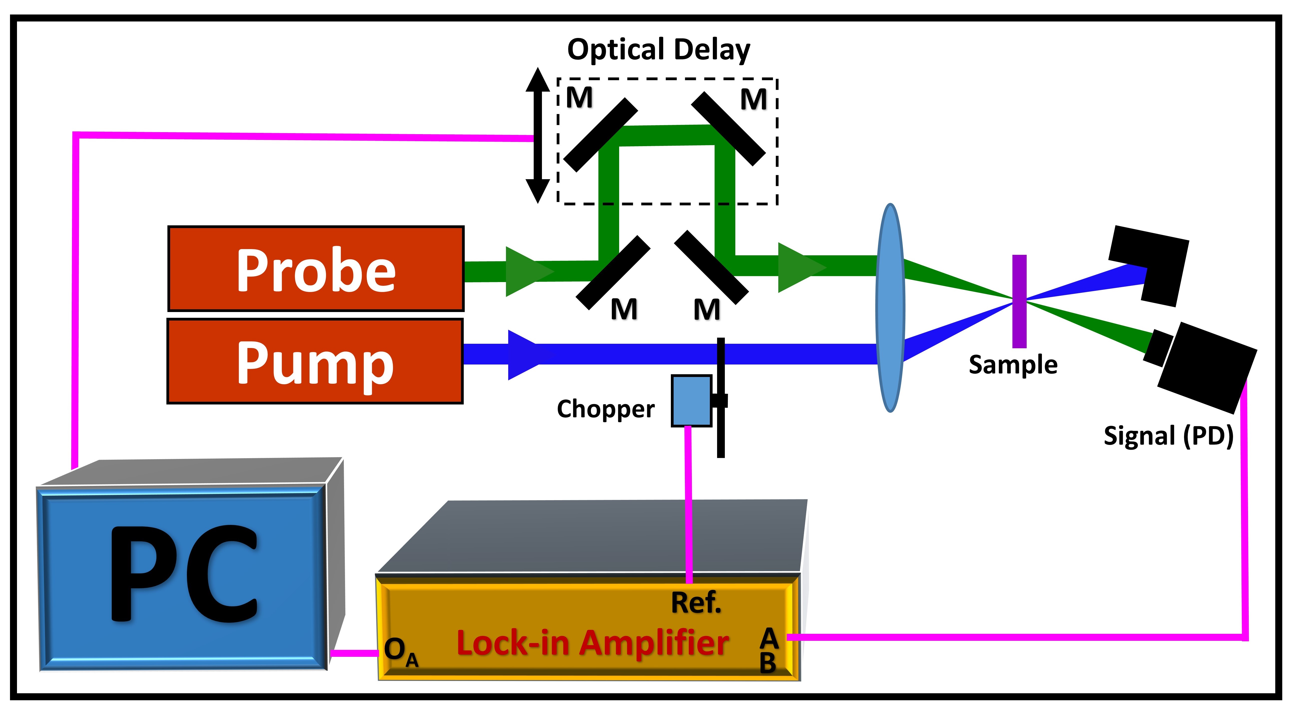
Figure 1: Schematic of a typical pump-probe setup used for the measurement of transient absorption based phase sensitive detection. M-Mirror and PD-Photodetector.

Consider a standard transient pump-probe measurement performed on a sample using time synchronized pump and probe pulses (Fig.1). In such measurements the change in the absorption/reflectivity of the sample is first measured at a given delay between the pump and probe pulses and this measurement is then repeated at several other delays to obtain the complete temporal responseNorris et al. (2003); Stevens et al. (2006). Let us consider a situation in which the laser source used in the measurement is highly stable and has sufficiently high pulse repetition rate. If the response time of the photodetector (PD) being used is slow compared to the pulse to pulse separation, then the output voltage of the PD will be a constant which is proportional to the average power of the laser beam being detected. Let $P_{in}$ be the average power of the probe beam falling on the front side of the sample (for simplicity reflection losses are neglected in this analysis). The output voltage of the PD detecting the transmitted power through the sample can be written as,

$$V_{O}(t)=CTP_{in}+Re\left[\sum_{\omega_{N}}V_{N}(\omega_{N})e^{-i\omega_{N}t}\right]$$ (1)

where $C$ is a constant which depends on the sensitivity of the PD and filters that are being used, $T$ is the transmission of the sample. $C$ will have the unit of A^-1. The second term accounts for the systematic and random electrical and optical noises in the measurement expressed in frequency domain. $V_{N}(\omega_{N})$ is the amplitude of the noise at frequency $\omega_{N}$. When the sample is excited by the pump pulse its optical response changes. For sufficiently small excitation conditions, the change in the absorption coefficient will be proportional to the third-order nonlinear absorption coefficientSutherland (2003); Jayabalan et al. (2009). Consider an instantaneously responding sample having a relaxation time much longer than the pulse width, the absorption coefficient after excitation by the pump pulse can be written as,

$$\alpha(E_{P},\tau)=\alpha_{0}+\beta(\tau)E_{P},$$ (2)

where $\alpha_{0}$ is the linear absorption coefficient, $E_{P}$ is the energy of the pump pulse, $\beta$ is related to the third-order nonlinear absorption coefficient with dimension of $1/(\alpha E_{P})$ and $\tau$ is the time between the excitation of the pump pulse and arrival of the probe pulse. It is the temporal evolution of $\beta$ which finally reveals the carrier dynamics in the sample. For a sufficiently small induced change in the optical response ($\alpha_{0}>>\beta E_{P}$), the transmission of the sample in presence of pump pulse is given by,

$$T =e^{-\alpha d},$$ (3)

$$\approx T_{0}\left[1-\beta(\tau)E_{P}d\right].$$ (4)

where $T_{0}$ is the linear transmission of the sample having thickness $d$ and is equal to $\exp(-\alpha_{0}d)$. The change in the transmission of the sample ($\Delta T=T-T_{0}$) induced by the pump pulse is given by,

$$\Delta T(\tau)=-T_{0}\beta(\tau)E_{P}d.$$ (5)

If the pump beam is modulated at a frequency $\Omega_{c}$, the transmission of the sample will also change at that frequency between $T_{0}(1-\beta E_{P}d)$ (when pump pulse is falling on the sample) and $T_{0}$ (when pump is blocked). To get a good S/N ratio the $\Omega_{c}$ has to be chosen such that the electrical and optical noise in the lab is least at this frequency. Thus the output voltage of the PD when the pump beam is modulated is given by,

$$V_{O}(t)=CT_{0}\left[1-\beta(\tau)E_{P}\mathcal{G}(t)d\right]P_{in}+Re\left[\sum_{\omega_{N}}V_{N}(\omega_{N})e^{-i\omega_{N}t}\right].$$ (6)

Here, $\mathcal{G}(t)$ is a the pump beam modulating function. Assuming a square wave modulation of the pump pulse, which is typical for the mechanical chopping of the pump beam, the modulating function $\mathcal{G}(t)$ can be expressed in terms of infinite sum of sinusoidal waves given byArfken and Weber (1999),

$$\mathcal{G}(t)=\frac{4}{\pi}\sum_{k=1}^{\infty}\frac{\sin\left[(2k-1)\Omega_{c}t\right]}{2k-1}.$$ (7)

In a phase sensitive detection technique the output of the PD is connected to the input of a lock-in-amplifier. Using the chopper frequency as the reference signal, the lock-in-amplifier will measure the amplitude of the voltage at $\Omega_{c}$. Substituting Eq.7 into Eq.6 the output of the lock-in amplifier, $V_{O}$, at the frequency $\Omega_{c}$ can be obtained and is given by,

$$V_{L}(\tau)=-\frac{4C}{\pi}T_{0}\beta(\tau)E_{P}P_{in}d.$$ (8)

As mentioned earlier the $\Omega_{c}$ is chosen such that there is negligible noise at that frequency, hence $V_{N}(\Omega_{c})\approx 0$. Using Eq.5 and Eq.8 the transient transmission at the delay $\tau$ can be written as,

$$\frac{\Delta T(\tau)}{T_{0}}=\frac{\pi}{4C}\frac{V_{L}(\tau)}{P_{in}T_{0}}.$$ (9)

A direct measurement of transmitted probe power though the sample using the same PD under similar condition by blocking the pump beam would produce a constant voltage, $V_{0}=CT_{0}P_{in}$, at the output of the PD. Using this Eq.9 can now be written as,

$$\frac{\Delta T(\tau)}{T_{0}}=\frac{\pi}{4}\frac{V_{L}(\tau)}{V_{0}}.$$ (10)

Thus by using the output of the lock-in-amplifier ($V_{L}$) at various delays and $V_{0}$ the transient transmission through the sample could be measured with high S/N ratio.

Repetition rate of several femtosecond oscillators are of the order of 80 MHz, which corresponds to a pulse to pulse separation of 12.5 ns. Typical PDs which has microsecond response times will give a DC output when irradiated with output of such high repetition rate lasers. By chopping the pump beam at few kHz, which is well away from the laser repetition rate and normal sources of noises, a good signal to noise ratio for the transient measurement could be obtainedJayabalan et al. (2009); KHAN et al. (2014). As mentioned in the introduction, many samples need higher pump pulse energies for generating sufficient change in probe as well as long pulse to pulse separation for providing sufficient time for the sample to relax. Femtosecond amplifier systems can provide much higher energies and are generally operated at $\sim$ 1 kHz which corresponds to a pulse to pulse separation of 1 ms. When pump-probe measurements are carried out using such beams, the separation between the chopping frequency and laser repetition rate is very less. Further $1/f$ noise, other unwanted electrical and optical noises become difficult to isolate when the chopper frequency is less than 1 kHz. When low repetition rate lasers are used for a pump-probe measurement the true signal arrives at the photodetector only for a very short duration, while rest of the time (much longer than the signal duration) the photodetector generates unwanted signal from dark current, stray light and other electrical noises. Such unwanted accumulation of noise can be removed if the signal is measured only at the time of pulse arrival and rest of the data are rejected. Boxcar is an electrical instrument which can detect the signal from a photodetector for a specific duration and produce a corresponding DC voltage at its output. The boxcar can be triggered by using a voltage pulse and it is possible to set a delay between the trigger and the measurement of signal. Boxcar also has provision to average the measured signal. P. Bartolini et al. reported a real-time acquisition system in which a balanced detector (for minimizing common-mode noise), a boxcar averager and a data acquisition board were used for pump-probe measurement using low-repetition rate laser Bartolini et al. (2007). For pump-probe measurements with high-repetition rate laser, they have replaced the boxcar with a lock-in-amplifier. Acquisition of large amount of data using data acquisition cards and post processing of the collected information with lot of averaging has also been used for improving signal to noise ratio Bartolini et al. (2007); Anderson et al. (2007); Werley et al. (2011); Sahoo et al. (2018). Here, we present a new detection technique by utilizing the merits of both the boxcar and lock-in-amplifier instruments and the same is shown to be very useful in case of pump-probe experiments performed with a low repetition rate (1 kHz) laser system.

III Experimental Details

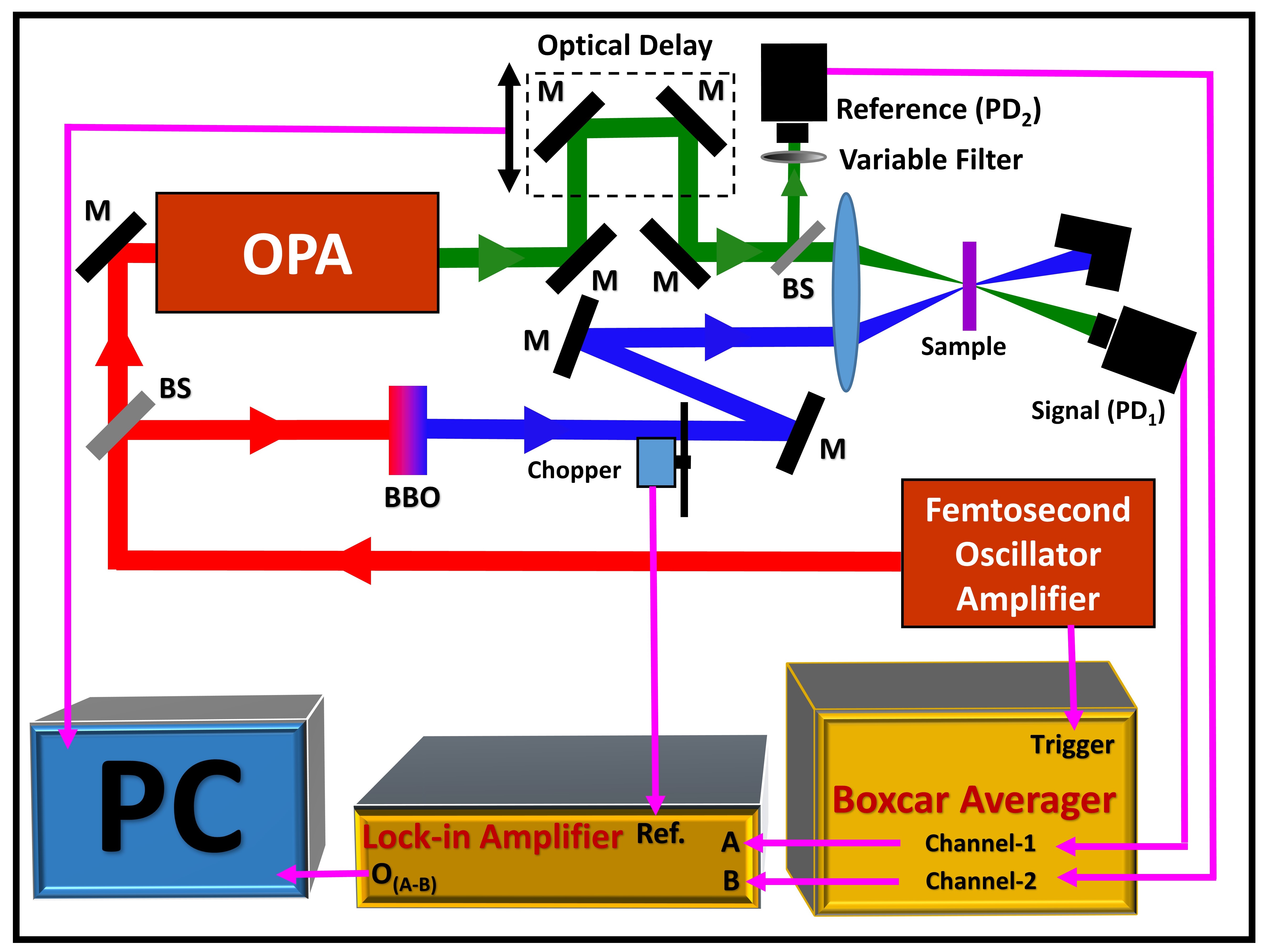
Figure 2: Schematic of the pump-probe setup along with the high sensitive detection system which combines advantages of boxcar and lock-in-amplifier. M-Mirror, BS-Beam Splitter, BBO-Beta Barium Borate crystal and PD-Photodetector.

For the demonstration of the present detection technique which combines the advantages of boxcar and lock-in-amplifier, pump-probe measurement was carried out on a Silver nanoparticle film by exciting at 400 nm and probing at 408 nm. Figure.2 shows the schematic diagram of the experimental setup along with the details of the detection scheme. The schematic of the pump-probe setup remains same as that shown in Fig.1 except for the detection of reference, but with a very different detection scheme which also incorporates a boxcar. The femtosecond oscillator-amplifier system delivers 35 femtosecond, 800 nm pulses at 1 kHz repetition rate. The 400 nm pump pulse was obtained by frequency doubling part of the 800 nm amplifier output using a Beta Barium Borate crystal (BBO). Another part of the amplifier output was used to pump an optical parametric amplifier (OPA). The typical standard deviation of the laser pulse-to-pulse energy fluctuation normalized to the average is nearly 3.4%. The output of the OPA when operated at 408 nm was used as the probe beam. The pump and probe pulses were spatially overlapped on the sample using a lens. The temporal delay between the pump and probe pulses is controlled by passing the probe beam through a optical delay line. The transmitted probe power is measured using a normal photodetector (PD₁). The peak change in the voltage pulse generated by the photodetector is proportional to the pulse energy. Due to the design of the PD₁, this voltage pulse decays nearly exponentially with a time constant of $\sim$ 20 $\mu$s. Using the trigger from the laser timing circuit and by suitably choosing the delay and width of gate pulse, a boxcar (Stanford Research System SR200 Series) is made to detect the peak change in the photodetector voltage. All the measurements were carried out by operating boxcar without any amplification and under no averaging condition. The output of the boxcar generates a corresponding constant voltage which is now proportional to the laser pulse power. This output is connected to the input of a lock-in-amplifier (Signal Recovery Model 7265). Under no averaging condition in the boxcar output will be a constant voltage which changes every 1 ms due to the 1 kHz repetition rate of the laser. If the laser pulse to pulse energy fluctuation is negligible, the output of the boxcar will be a constant which is now nearly independent of repetition rate of the laser. Thus by inserting a boxcar in between the output of the PD₁ and lock-in-amplifier an experiment performed using a low-repetition rate laser has been converted to a situation which is similar to the constant output obtained from a slow photodetector when exposed to a high-repetition rate laser. In addition, the boxcar can also remove any noise that is time shifted with respect to the pulse arrival, the sharp electrical pickup noise which occur due to the pulse switch out process in the amplifier. Further, the response time of PD itself would not matter since the boxcar can be made to pickup the signal at a specific time on the output of PD signal.

Now the pump beam is mechanically chopped at a specific frequency ($\Omega_{c}$). If the laser pulse arrives at the chopper when the chopper blade is partially blocking the beam path the pulse will get cut spatially creating unwanted changes in the pump pulse energy and random beam profile changes. To reduce such noise the chopper is placed at a location where the diameter of the beam is least. The output of the boxcar is connected to the channel A of the lock-in-amplifier. The pump-induced change in the transmission of the sample will modulate the boxcar output at the chopper frequency which can now be detected by the lock-in-amplifier as described in section II.

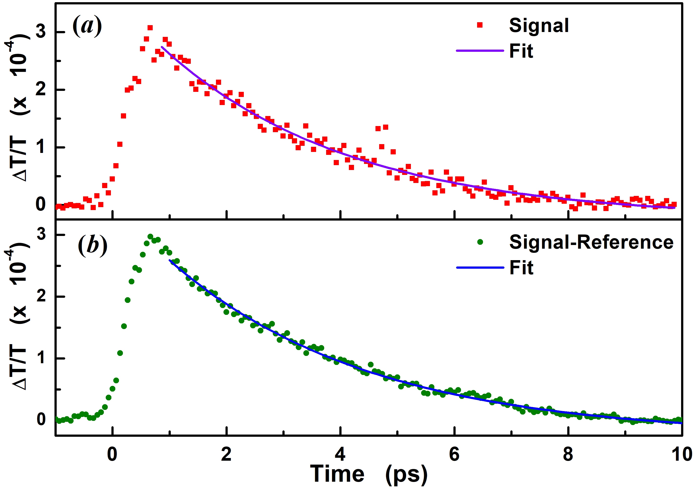
Figure 3: Transient transmission signal measured of a Ag thin particulate film. (a) the output of PD₁ is detected by boxcar and the output of boxcar is then sensed with lock-in-amplifier at chopper frequency and (b) similar to (a) except that the fluctuation in the signal is further reduced by subtracting a reference probe signal (see the text for details).

Figure 3 (a) shows the measured transient transmission of the Ag thin film sample performed by the present detector configuration. The chopping frequency was chosen to be 405 Hz. With the arrival of the pump pulse the transmission through the sample increases. In Ag nanoparticles the change in the transmission which is caused by the electron-phonon thermalization recovers in next few picosecondsMuskens et al. (2006); Jayabalan et al. (2009); Singh et al. (2019). A single exponential fit to the decay part of the signal gives a decay time of 3.3 $\pm$ 0.2 ps. Such transient response is typical for a metal nanoparticles.

In order to study the statistical variation in the signal among various pump-probe detection parameters, the signal at the peak of the transient transmission ($\approx$ 0.5 ps) was recorded repeatedly. Then an estimate for the statistical variation ($S_{D}$) in percentage is calculated using,

$$S_{D}=100\times\sqrt{\frac{1}{N}\sum_{i=1}^{N}\left(\frac{S_{i}}{S_{av}}-1\right)^{2}},$$ (11)

where $N$ is the number of data points, $S_{i}$ represents the individual measured data and $S_{av}$ is the average defined by,

$$S_{av}=\frac{1}{N}\sum_{i=1}^{N}S_{i}.$$ (12)

Since the data is normalized to the average, lower value of $S_{D}$ implies a good S/N ratio. The $S_{D}$ estimated for the signal measured at the peak of $\Delta T/T$ shown in Fig.3 (a)) is 27 (N = 100).

If the pulse to pulse power fluctuation in the laser is negligible, the collected data can be considered as similar to that of a standard transient transmission measurement performed using a high-rep rate laser. Generally the pulse to pulse energy stability of femtosecond amplifier system is much poorer when compared to that of oscillators. Thus the transient signal measured using this low repetition rate oscillator-amplifier-OPA system will have additional noise due to pulse to pulse energy fluctuation. In the following we show, first theoretically and then experimentally the effect of such pulse to pulse energy variation in the probe pulse on the S/N ratio and a method to counter it.

Let the average pulse energy of the probe pulse at the input of the sample be $E_{in}$ with a random pulse to pulse energy fluctuation $\Delta E_{in}$. The value of $\Delta E_{in}$ would change at every 1 ms in a 1 kHz repetition rate system. The distribution of $\Delta E_{in}$ for a ensemble of pulses would be a Gaussian, which is typical for the type of laser used in the present measurement. The voltage output of the boxcar channel which is detecting the transmitted probe pulse through the sample using PD₁ is,

$$V^{B}_{O}(t)=C^{B}T\left[E_{in}+\Delta E^{in}\mathcal{H}(t)\right]+Re\left[\sum_{\omega_{N}}V^{B}_{N}(\omega_{N})e^{-i\omega_{N}t}\right].$$ (13)

where $C^{B}$ is a constant which depends on the sensitivity of the PD₁ and gain in the boxcar. $V^{B}_{N}$ is the amplitude of electrical and optical noise at frequency $\omega_{N}$. Once again for small change in the transmission of the sample in presence of pump pulse ($E_{P}$) modulated by a function $\mathcal{G}(t)$, the output of the boxcar can be written as,

$$V^{B}_{O}(t)=C^{B}T_{0} \left[1-\beta(\tau)E_{P}\mathcal{G}(t)d\right]\left[E_{in}+\Delta E_{in}\mathcal{H}(t)\right]$$

$$+Re\left[\sum_{\omega_{N}}V^{B}_{N}(\omega_{N})e^{-i\omega_{N}t}\right].$$ (14)

Here, $\mathcal{H}(t)$ is a unit step function which repeats with the arrival of probe pulse. Since $\Delta E_{in}$ varies randomly depending on the energy of each probe pulse, the product of $\Delta E_{in}$ and $\mathcal{H}(t)$ will be composed of several frequencies and can also have component at the chopper frequency.

For sufficiently small fluctuations in the probe energy $\Delta E_{in}<<E_{in}$, the term containing the product of $\beta$ and $\Delta E_{in}$ in Eq.14 can be neglected when compared to the other terms. Thus the output of the lock-in-amplifier which is now detecting the BC output in channal A can be written as,

$$V^{B}_{L}(\tau)= -\frac{4C^{B}}{\pi}E_{in}T_{0}\beta(\tau)E_{P}d+\Delta E_{in}\mathcal{F}(t)C^{B}T_{0}$$ (15)

where $\mathcal{F}(t)$ is the amplitude of Fourier transform of $\Delta E_{in}\mathcal{H}(t)$ at the chopping frequency and it depends on time because of the slow variations in laser pulse energy. Note that the second term in the Eq.15 does not depend on the $\beta(\tau)$ of the sample, however depends directly on the pulse to pulse fluctuation. Thus, due to shot to shot energy fluctuation in probe, additional noise (given by second term in Eq.15) will get added to the required signal, the first term. The $\Delta T/T$ presented in Fig.3 will have fluctuations caused by the random probe energy variation.

For removing this noise a small part of probe beam was reflected before the sample and was detected using another photodetector (PD₂). The output of the PD₂ is also processed by another channel of the boxcar. The output of the boxcar can be written as,

$$V^{B2}_{O}(t)=C^{B2}T_{f}R\left[E_{in}+\Delta E_{in}\mathcal{H}(t)\right]+Re\left[\sum_{\omega_{N}}V_{N}^{B2}(\omega_{N})e^{-i\omega_{N}t}\right],$$ (16)

where $C^{B2}$ is a constant which depends on the sensitivity of the PD₂ and gain in boxcar. $R$ is the reflectance of the beam splitter used for obtaining the reference beam and $T_{f}$ is the transmission of filter used before PD₂. Using a variable filter, the $T_{f}$ was chosen such that $C^{B2}RT_{f}=C^{B}T_{0}$ (one can also change the gain in the boxcar channel detecting the output of PD₂). This can be easily done directly by monitoring the boxcar outputs $V^{B}_{O}(t)$ and $V^{B2}_{O}(t)$ in an oscilloscope and making them almost equal. This voltage $V^{B2}_{O}(t)$ is then subtracted to the boxcar output of PD₁ ($V^{B}_{O}(t)$) electronically before feeding in to the lock-in-amplifier. Most of the commercial lock-in-amplifier do come with a provision for such subtraction (channel B) of voltage which could be directly used for this subtraction purpose. The output voltage after subtraction (A-B) can be written as,

$$V^{D}_{O}(t)=-C^{B}T_{0}\beta(\tau)E_{P}\mathcal{G}(t)d\left[E_{in}+\Delta E_{in}\mathcal{H}(t)\right]$$

$$+Re\left[\sum_{\omega_{N}}(V^{B}_{N}-V^{B2}_{N})e^{-i\omega_{N}t}\right].$$ (17)

The output of the lock-in-amplifier which is now detecting the $V^{D}_{O}(t)$ using the chopping frequency as reference will be,

$$V^{B}_{L}(\tau)= -\frac{4C^{B}}{\pi}E_{in}T_{0}\beta(\tau)E_{P}d,$$ (18)

A direct measurement of transmitted probe pulse energy though the sample using the same PD₁ under similar condition through the boxcar by blocking the pump beam would produce a constant voltage, $V^{B}_{D}=C^{B}T_{0}E_{in}$ at the output of the boxcar. Now using Eq.5 and the measured $V^{B}_{D}$ the transient transmission through the sample can estimated by,

$$\frac{\Delta T(\tau)}{T}=\frac{\pi}{4}\frac{V^{B}_{L}(\tau)}{V^{B}_{D}}.$$ (19)

It is important to note that in the present technique usage of an identical balanced detector is not essential as done by several earlier reports. Normal photodetectors can be used for measuring the reference and signal to reduce the noise due to probe energy fluctuations. Only the DC output of boxcar needs to be made equal ($V^{B}_{O}(t)$ = $V^{B2}_{O}(t)$).

Figure 3 (b) shows the measured transient transmission signal of the metal thin film sample performed by the A-B configuration. A single exponential fit to the decay part of this signal gives a decay time of 3.5 $\pm$ 0.1 ps. The $S_{D}$ of signal measured at the peak change in the present case is 10, which is nearly one third of that when the signal measured without subtraction of boxcar output of PD₂ from that of PD₁.

Table 1: The dependence of $S_{D}$ and peak to peak variation in the signal at different chopper frequencies $\Omega_{c}$ around 333 Hz.

$\Omega_{c}$	$S_{D}$ (%)	Peak to Peak fluctuation (%)
230	15.5	95.3
280	13.9	56.6
333	2.9	14.5
380	11.5	44.6
420	11.6	61.2

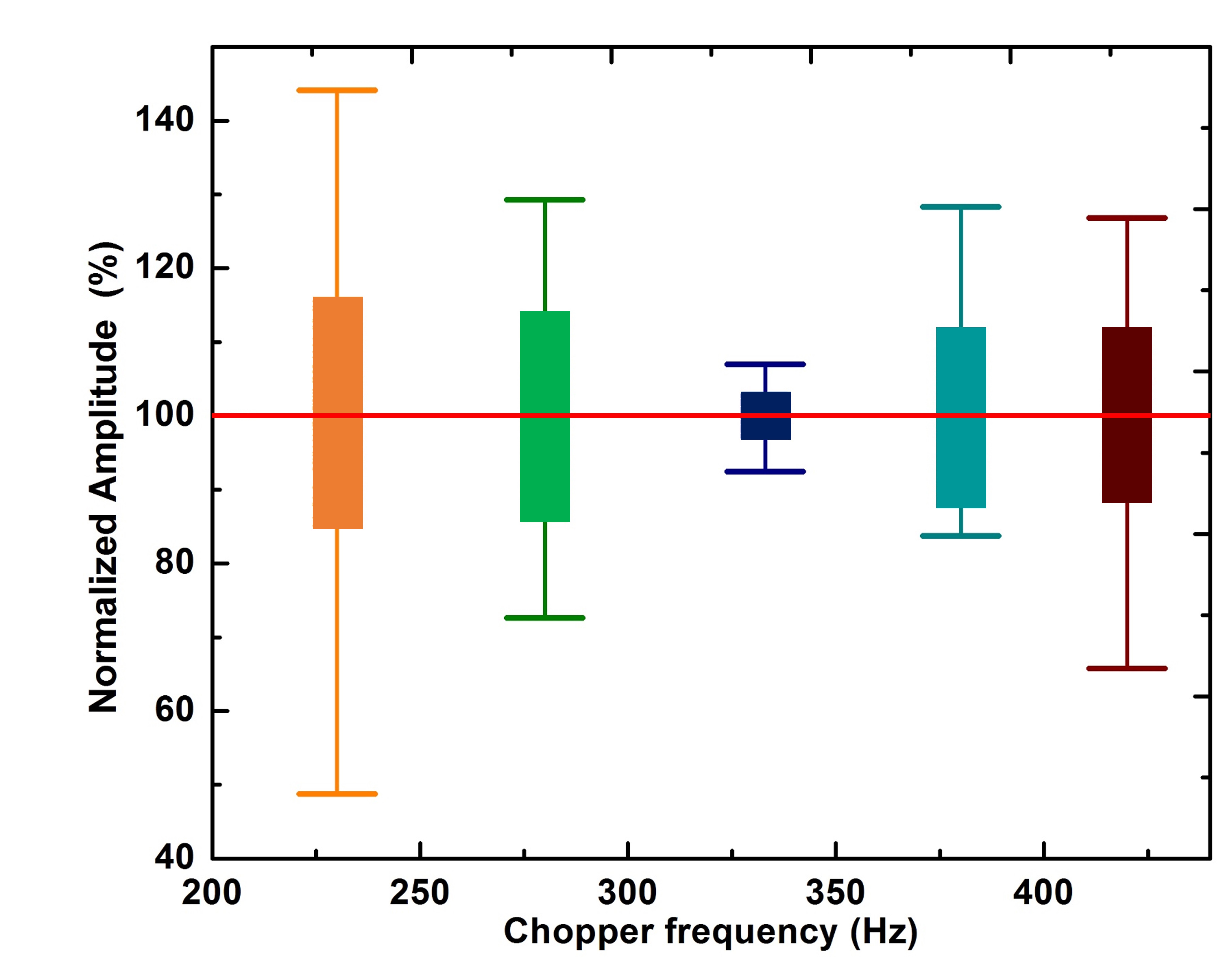
Figure 4: The dependence of the fluctuations in the normalized signal measured at peak position in A-B configuration on the chopping frequencies around 333 Hz. The height of the rectangular box represents the $S_{D}$ and the maximum and minimum signals values in the data set are also shown as bar.

To further reduce the statistical fluctuations in the measurement, a chopper frequency dependent study was carried out on the same sample. The transient signal at the delay where peak occurs is recorded repeatedly in the A-B configuration ($N$ is $\sim$ 100) at various chopper frequencies. The statistical variation in the peak signal as given by Eq.11 was estimated at each chopper frequencies and are given in Table.1. Further apart from $S_{D}$ it is also important to know about maximum and minimum signal obtained in the measured data to understand the stability in the measured signal. Figure.4 shows the variation of $S_{D}$ on the chopping frequencies as a solid rectangle. The Fig.4 also shows the measured maximum and minimum signal values among the data set at each chopper frequency as bars. Clearly the $S_{D}$ is least for the chopping frequency 333 Hz. As the chopper frequency deviates away from 333 Hz we find that the $S_{D}$ and the peak to peak variation in the signal also increases.

Table 2: The dependence of $S_{D}$ and peak to peak variation in the signal at different chopper frequencies which are factors of 1 kHz.

$\Omega_{c}$	$S_{D}$ (%)	Peak to Peak fluctuation (%)
200	12.0	52.8
250	9.8	46.2
333	2.9	14.5
500	12.0	58.0

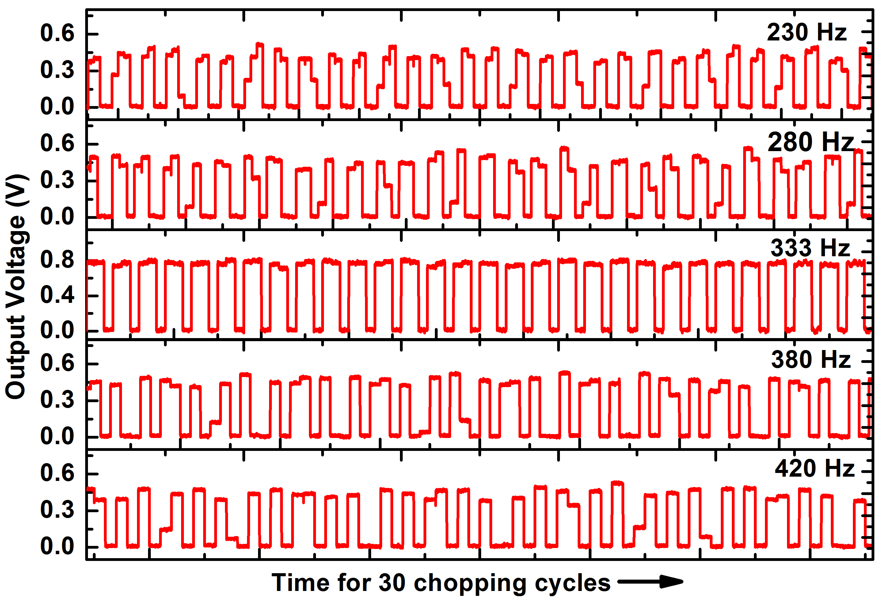
Figure 5: Output voltage of the boxcar which is measuring the output of the photodetector sensing pump pulses passing though the chopper operated at different frequencies. The time in the horizontal axis at each chopping frequency is chosen such that there are 30 chopping cycles in view.

When the laser pulse repetition rate is very large compared to the chopping frequency, the number of laser pulses blocked or unblocked in each cycle would remain nearly same. On the other hand, when the laser repetition rate and the chopper frequency is close an temporal aliasing process can lead to frequent changes in the number of pump pulses which are actually getting passed though the chopper. To measure the effect of chopper on the pump pulses we have directly measured the energy of the pump pulses after passing through the chopper. Fig.5 shows the output of the boxcar measuring the output of the photodetector detecting the modulated pump-pulses passing though the chopper for 30 cycles. Here zero amplitude means that the chopper had blocked the pulse while the higher amplitudes corresponds to the energy of the pulses passing through the chopper. Clearly the pump pulses are getting partially blocked by the chopper at frequencies other than 333 Hz. This phenomena can also be explained as follows. The chopper frequency 333 Hz is a factor of the laser repetition rate, 1 kHz. Thus in each chopper cycle two pulses are passed and one pulse is blocked and the process repeats (the reverse, two pulses are blocked and one pulse is passed is also possible depending on the starting time of chopper). On the other hand, if the chopper frequency is such that it is not a factor of laser repetition rate then frequently the chopper blade would be in a partially closed or partially open condition during the pulse arrival. Such partial cutting of pump pulse would lead to strong changes in the pump energy as well as spatial shape distortion of the beam profile at the sample place. Since the transient signal is proportional to the pump pulse energy (see Eq.18), these variations would cause signal to fluctuate. Thus, 333 Hz is one of the possible factor of 1 kHz which can have least fluctuation in the signal as well as least variation in peak to peak. Hence, to avoid such chopping generated modulations in the pump pulse it is essential chose the chopping frequency as one of the factor of the laser repetition rate.

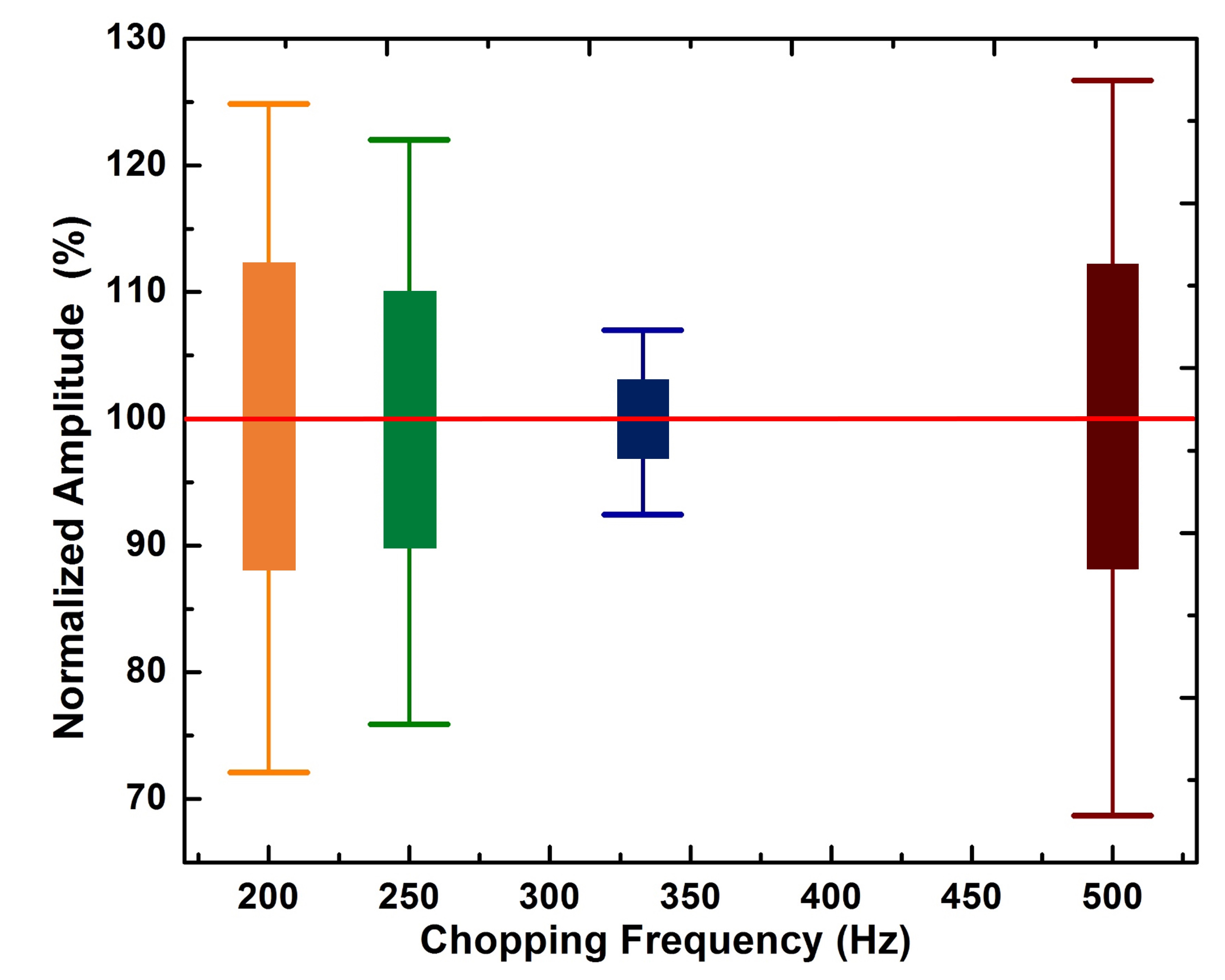
Figure 6: The dependence of the fluctuations in the normalized signal measured at peak position in A-B configuration on the chopping frequencies which are factors of 1 kHz. The height of the rectangular box represents the $S_{D}$ and the maximum and minimum signals values in the data set are also shown as bar.

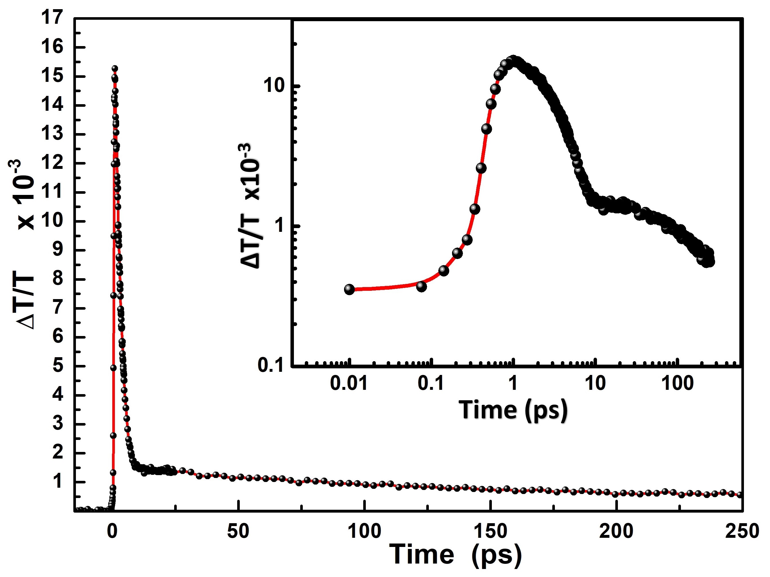
Figure 7: A typical transient absorption signal measured with 333 Hz chopping. Inset shows the same curve in log-log scale.

We have also performed similar measurement at all the chopper frequencies which are factors of 1 kHz in the A-B configuration. The statistical variation in the peak signal are given in Table.2. Figure.6 shows the dependence of $S_{D}$ and the measured maximum and minimum signal values on the harmonic chopping frequencies which are factors of 1 kHz. Once again the $S_{D}$ for the case of chopping frequency 333 Hz has the least $S_{D}$. Although the chopper frequencies, 200 Hz, 250 Hz and 500 Hz are factors of 1 kHz still the noise at these frequencies are much higher than that of 333 Hz. Pump-probe measurements performed at very low chopper frequencies like 50 or 100 Hz (factors of 1 kHz) result in increasing the shot-to-shot fluctuations leading to even lower signal-to-noise ratio. The AC power supply frequency which is being used in the experiment is 50 Hz and the on-off frequency of most of the laboratory light sources are driven by this AC power supply is 100 Hz. Thus, because of any kind of stray light present in the lab, it is well known that 50 Hz, 100 Hz and their higher harmonics are all not suitable for chopping frequencies. When chopped at these frequencies the lock-in-amplifier will sense these electronic noises or the other light which are being detected by the photodetectors. Since the chopping frequencies 200 Hz, 250 Hz and 500 Hz are all higher harmonics of 50 Hz and 100 Hz the signal detected at these frequencies will have higher noise compare to that at 333 Hz. Several earlier reports used 500 Hz or various other chopping frequencies for the measurement of pump-probe signal with 1 kHz systemGonçalves et al. (2016); Werley et al. (2011); Sahoo et al. (2018). Our result suggests that for a best S/N ratio, the pump should be chopped at 333 Hz. Further, even for the case where only lock-in-amplifier is used in the measurement the chopping has to be done at 333 Hz. Although the technique reported here takes care of the fluctuations in data caused by the probe energy variation, still the variations in pump energy would cause the signal to vary (Eq.18). Figure.7 shows an transient absorption signal measured on a silver nanoparticle sample under fully optimized conditions and averaged over 8 measurements at each delay. In such long delay range a second slow decay in the transient signal which is due to the phonon-phonon interaction can also be clearly identified (see the inset of Fig.7) Muskens et al. (2006); Jayabalan et al. (2009).

IV Conclusion

In this work, a detection scheme which combines the advantages of boxcar and lock-in-amplifier for performing pump-probe using low-repetition rate laser system was demonstrated. A theoretical model was developed to explain the process of signal detection. The boxcar was operated such that it detects the peak signal from the photodetectors avoiding any noises that are being picked up by the photodetectors thus isolating noise in time domain. Chopping the pump and detecting the output of the boxcar using a lock-in-amplifier provides a way to isolate other electrical and optical noises that generally appear at other frequencies. In addition these noise isolations, a way to reduce the signal fluctuations due to pulse to pulse probe energy variation was also shown experimentally. A chopping frequency dependent study shows that for best signal to noise ratio the chopper frequency should be a factor of the laser repetition rate. Further, it should not also be a harmonic of the AC power supply. Thus in case of low-repetition rate lasers, it is not only essential to move away from harmonics of AC supply, but also to a frequency which is a factor of its repetition rate. Further, we also find that the gain in boxcar could also be used to increase the signal without much change in the S/N ratio.