Deep Learning, Predictability, and Optimal
Portfolio Returns

Abstract

We study dynamic portfolio choice of a long-horizon investor who uses deep learning methods to predict equity returns when forming optimal portfolios. Our results show statistically and economically significant benefits from using deep learning to form optimal portfolios through certainty equivalent returns and Sharpe ratios. We demonstrate that a long-short-term-memory recurrent neural network, which excels in learning complex time-series dependencies, generates a superior performance among a variety of networks considered. Return predictability via deep learning generates substantially improved portfolio performance across different subsamples, particularly during recessionary periods. These gains are robust to including transaction costs, short-selling and borrowing constraints.
Keywords: Return Predictability, Portfolio Allocation, Machine Learning, Neural Networks, Empirical Asset Pricing

JEL codes: C45, C53, E37, G11, G17

1 Introduction

Extensive empirical asset pricing literature has documented supportive evidence for equity return predictability. With an ever increasing number of potential predictors, the practice of applying machine learning methods to make the most accurate predictions using large datasets is gaining further traction. This new literature demonstrates superior performance of machine learning approaches relative to the linear regression analysis researchers favor due to its simplicity. However, it is unclear whether sound statistical performance of machine learning leads to portfolio gains for an investor who applies these models of return predictability when forming optimal portfolios.

In this paper, we examine the economic value of non-linear machine learning methods, such as neural networks (NNs), for an investor forming optimal portfolios. We study the asset allocation of a long-horizon investor with a power utility choosing between a market portfolio and a risk-free asset. Our optimal portfolio design exercise follows Johannes et al., (2014) and our statistical comparison is similar to Gu et al., (2020). To this end, we implement a variety of machine learning architectures including shallow and deep feedforward NNs, as well as long-short-term-memory (LSTM) recurrent NNs. On the methodology side, while there is an extensive literature on statistical and economic significance of standard feedforward NNs exploring information contained in cross-section of returns, we are the first to explore the LSTM recurrent NNs that are more suitable for prediction of time series. We argue that time series dependence is important feature to be explored and we document that LSTM recurrent NNs being able to identify time-series dependence deliver larger portfolio gains. The reason for the documented gains is that an LSTM is a specialized form of a neural network, which is capable of learning complex long-term temporal dynamics and hence explore the time series dependence that vanilla NN is unable to learn.

Our contribution to the portfolio literature is threefold. First, we show that using machine learning methods for the construction of optimal portfolios generates economically significant gains. Specifically, we document that deviating from the Expectations Hypothesis and using NNs to forecast excess returns results in three times higher Sharpe ratios (SRs) and twice as high certainty equivalent returns (CERs). This evidence contributes to the debate on the economic value of equity return predictability (Goyal and Welch,, 2008; Johannes et al.,, 2014; Rossi,, 2018). Furthermore, our evidence on the benefits of NNs is robust to alternative measures of portfolio performance (cumulative return, maximum drawdown, and maximum one-month loss) and to the inclusion of transaction costs, short-selling and borrowing constraints. Our results are consistent with Johannes et al., (2014) who report significant portfolio benefits from second-moment temporal dependence in equity returns. Using machine learning allows us to explore even more complex dependencies in a model-free way.

Moreover, dissecting the economic gains of NNs across subsamples, we find that, historically, machine learning methods generate the highest CERs in each of the seven decades in the post-WWII period. Interestingly, NNs generate on average twice larger SRs during NBER recessions compared to the periods of expansion. In particular, we find that all NNs are able to generate significant gains during the 2007-2008 Financial Crisis. Finally, an investor benefits more from NNs by rebalancing her portfolio more frequently, as opposed to applying a passive strategy. We show that the gains are not eliminated by the increased turnover.

Second, compared to the existing evidence for linear models, deep learning methods provide a single “silver bullet” by generating out-of-sample gains without relying on additional ingredients. We demonstrate that portfolio performance when using NNs dominates strategies using the linear predictive models even when time-varying return volatility is omitted. Our evidence is consistent with Goyal and Welch, (2008) and Johannes et al., (2014) in that we also do not identify benefits from using linear models without estimation risk and time-varying volatility. We contribute to the literature by showing that the empirical evidence for the predictability of equity returns is economically significant even in the absence of these additional ingredients, provided the investor uses non-linear machine learning methods to detect this predictive variation.

Our third contribution is related to the properties of economic gains implied by NNs. We find that increasing the complexity of deep learning architectures does not necessarily translate into improved portfolio performance. We document that moving from shallow settings with one hidden layer to deeper specifications does not result in additional gains. This seems to be a surprising result, but finance and return predictions in particular operate in a challenging data environment that differs substantially from other domains where deep learning results in large improvements. Specifically, return predictions with the goal of optimal portfolio construction is a small sample problem with the data facing very low signal-to-noise ratio (Israel et al.,, 2020) and increased network complexity does not necessarily help. Importantly, we document that inclusion of deep recurrent LSTM networks that capture important temporal dynamics improves performance according to all portfolio performance measures we consider. In this respect, our paper contributes to the evidence on economic information captured by NNs. Specifically, we extend the evidence presented by Rossi, (2018) for boosted regression trees and show that, apart from the important non-linear relationship, long-term memory effects are particularly beneficial in short samples.

The remainder of this paper is organized as follows. Section 2 discusses standard approaches to assessing expected return predictability, introduces non-linear machine learning methods we consider, describes the portfolio choice problem of an investor, and outlines a variety of performance measures. Section 3 describes the data and summarizes the results. Section 4 dissects the economic gains from using NNs across subperiods and provides robustness checks to using alternative performance measures or including transaction costs, borrowing and short-selling constraints. Section 5 concludes.

2 Evaluating Predictability via Portfolio Performance

2.1 The Simple Linear Approach

The standard approach used to forecast excess equity returns is a linear model of the form

$$r_{t+1}=\mbox{\boldmath$\alpha$}+\mbox{\boldmath$\beta$}\mbox{\boldmath$x$}_{t}+\varepsilon_{t+1}^{r},$$ (1)

where $r_{t+1}$ are monthly log excess returns, $\alpha$ and $\beta$ are coefficients to be estimated, $\mbox{\boldmath$x$}_{t}=(\mbox{\boldmath$x$}_{t}^{1},...,\mbox{\boldmath$x$}_{t}^{n})$ is a set of predictor variables, and $\varepsilon_{t+1}^{r}$ is a normal error term. A large strand of empirical literature has examined linear regression models with multiple predictors including prominent variables such as the dividend yield, valuation ratios, various interest rates and spreads, among others. Although researchers have proposed numerous variables for predicting stock market returns, empirical evidence on the degree of predictability is mixed at best. Goyal and Welch, (2008) find that most linear specifications with multiple predictors perform poorly and remain insignificant even in-sample. They further show that an investor using linear models to forecast equity returns would not be able to improve portfolio performance compared to no predictability benchmark.

There are several reasons for the lack of robust evidence on the predictability equity returns and its benefits for portfolio construction. The specification defined by Eq.(1) assumes a linear and time-invariant relationship between log excess returns and predictors, which is at odds with the theoretical and empirical evidence. Bayesian learning about uncertain parameters in the linear regression has been proposed as a way to introduce a time-varying relationship between the returns and predictor variables. However, sequential parameter learning leads to significant portfolio benefits only in the presence of a highly informative prior (Wachter and Warusawitharana,, 2009) or a combination of estimation risk and time-varying volatility (Johannes et al.,, 2014). Thus, prior knowledge about the nature of expected return predictability or careful modeling of its conditional features, especially time variation in return volatility, are critical for generating economic gains.

This paper follows an alternative approach inspired by the recent development of machine learning in empirical asset pricing literature. Specifically, we apply neural networks to approximate the functional association between the set of predictors and returns for optimal portfolio construction. In doing so, we do not impose a known form of this relationship, but instead allow for flexible identification of potentially nonlinear interactions from the data. Our choice of neural networks over other machine learning methods (for instance, tree-based approaches) is motivated by the fact that they deliver the most accurate statistical performance, as documented by the existing literature. The aim of this paper is to revisit the evidence documented by Goyal and Welch, (2008) and to show that, unlike linear predictive regressions, sound statistical performance of neural networks indeed translates into substantial portfolio improvements for an investor using these novel methods when dynamically forming an optimal portfolio.

2.2 From Linear Regression Towards Deep Learning

Machine learning has a long history in economics and finance (Hutchinson et al.,, 1994; Kuan and White,, 1994; Racine,, 2001; Baillie and Kapetanios,, 2007). At its core, one may perceive machine learning as a general statistical analysis that economists can use to capture complex relationships that are hidden when using simple linear methods. Breiman et al., (2001) emphasize that maximizing prediction accuracy in the face of an unknown model differentiates machine learning from the more traditional statistical objective of estimating a model assuming a data generating process. Building on this, machine learning seeks to choose the most preferable model from an unknown pool of models using innovative optimization techniques. As opposed to traditional measures of fit, machine learning focuses on the out-of-sample forecasting performance and understanding the bias-variance tradeoff; as well as using data driven techniques that concentrate on finding structures in large datasets.

While finance is focused on expected return predictability, the ability of machine learning techniques to find relationships in data seems well-suited for financial applications. Further, if one dismisses the “black-box” view of machine learning as a misconception (Lopez de Prado,, 2019), it seems nothing should stop a researcher from exploring the power of these methods in financial data. However, problems in finance differ from typical machine learning applications in many aspects. In order to enjoy the benefits of machine learning, a user needs to understand key challenges brought by financial data.

Israel et al., (2020) note that machine learning applied to finance is challenged by small sample sizes, naturally low signal-to-noise ratios making market behavior difficult to predict and the dynamic character of markets. Because of these critical issues, the benefits of machine learning are not so obvious as in other fields and research into understanding how impactful machine learning can be for asset management is just emerging. With the surge in deep learning literature, machine learning applications in finance have begun to emerge (Heaton et al.,, 2017; Feng et al.,, 2018; Bryzgalova et al.,, 2019; Bianchi et al.,, 2020; Chen et al.,, 2020; Gu et al.,, 2020; Tobek and Hronec,, 2020; Zhang et al.,, 2020). Here we describe the core ideas we use for building deep learning models to predict the returns.

2.2.1   (Deep) Feedforward Networks

Figure 1: (Deep) Feedforward Network

This figure illustrates a deep neural network model $r_{t+1}=\mathfrak{f}_{W,b}(x_{t})+\varepsilon_{t+1}^{r}$ that predicts output return $r_{t+1}$ using a set of predictor variables $x_{t}=(x_{t}^{1},...,x_{t}^{n})$. The network is deep, with a number of hidden layers $L$.

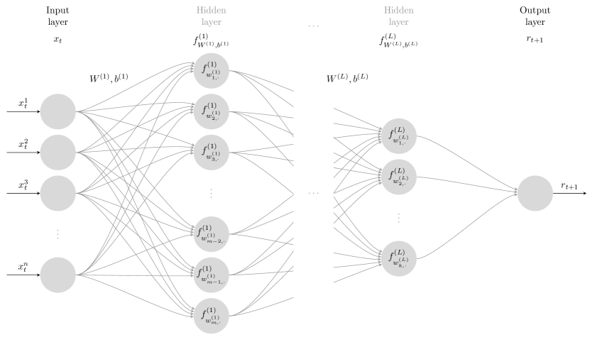
Deep feedforward networks, also often called feedforward neural networks, or multilayer perceptrons lie at heart of deep learning models and are universal approximators that can learn any functional relationship between input and output variables with sufficient data.

A feedforward network is a form of supervised machine learning that uses hierarchical layers to represent high-dimensional non-linear predictors in order to predict an output variable. Figure 1 illustrates how $\ell\in\{1,\ldots,L\}$ hidden layers transform input data $x_{t}=(x_{t}^{1},...,x_{t}^{n})$ in a chain using a collection of non-linear activation functions $f^{(1)},\ldots,f^{(L)}$. More formally, we can define our prediction problem by characterizing excess equity returns as:

$$r_{t+1}=\mathfrak{f}_{W,b}(x_{t})+\varepsilon_{t+1}^{r},$$ (2)

where $x_{t}=(x_{t}^{1},...,x_{t}^{n})$ is a set of predictor variables that enter an input layer, and $\varepsilon_{t+1}^{r}$ is i.i.d. error term, $\mathfrak{f}_{W,b}$ is a neural network with $L$ hidden layers such as

$$\widehat{r}_{t+1}:=\mathfrak{f}_{W,b}(x_{t})=f^{(L)}_{W^{(L)},b^{(L)}}\circ\ldots\circ f^{(1)}_{W^{(1)},b^{(1)}}\left(x_{t}\right),$$ (3)

and $W=\left(W^{(1)},\ldots,W^{(L)}\right)$ and $b=\left(b^{(1)},\ldots,b^{(L)}\right)$ are weight matrices and bias vector. Any weight matrix $W^{(\ell)}\in\mathbb{R}^{m\times n}$ contains $m$ neurons as $n$ column vectors $W^{(\ell)}=[w_{\cdot,1}^{(\ell)},\ldots,w_{\cdot,n}^{(\ell)}]$, and $b^{(\ell)}$ are a threshold or activation level that contribute to the output of a hidden layer, allowing the function to be shifted. Commonly used activation function $f^{(\ell)}_{W^{(\ell)},b^{(\ell)}}$

$$f^{(\ell)}_{W^{(\ell)},b^{(\ell)}}:=f_{\ell}\left(W^{(\ell)}x_{t}+b^{(\ell)}\right)=f_{\ell}\left(\sum_{i=1}^{m}W^{(\ell)}_{i}x_{t}+b_{i}^{(\ell)}\right)$$ (4)

are sigmoidal (e.g. $f_{\ell}(z)=1/(1+\exp(-z))$) or $f_{\ell}(z)=\tanh(z)$, or rectified linear units (ReLU) ($f_{\ell}(z)=\max\{z,0\}$). Note that in case functions $\mathfrak{f}$ are linear, $\mathfrak{f}_{W,b}(x_{t})$ is a simple linear regression, regardless of the number of layers $L,$ and hidden layers are redundant. For example with $L=2$, the model becomes a reparametrized simple linear regression: $\widehat{r}_{t+1}=W^{(2)}(W^{(1)}x_{t}+b^{(1)})+b^{(2)}=\beta x_{t}+\alpha.$ In case $\mathfrak{f}_{W,b}(x_{t})$ is non-linear, neural network complexity grows with increasing $m$, and with increasing the number of hidden layers $L$, or growing deepness of the network, we have a deep neural network.

2.2.2   (Deep) Recurrent Networks

Many predictors used in finance are non-i.i.d., and dynamically evolve in time, and hence traditional neural networks assuming independence of data may not approximate relationships sufficiently well. Instead, a Recurrent Neural Network (RNN) that takes into account time series behavior may help in the prediction task. In addition, Long-Short-Term-Memory (LSTM) is designed to find hidden state processes allowing for lags of unknown and potentially long time dynamics in the time series. Figure 2 illustrates how the network structure additionally uses lagged information.

More formally, RNNs are a family of neural networks used for processing sequences of data. They transform a sequence of input predictors to another output sequence introducing lagged hidden states as

$$h_{t}=f(W_{h}h_{t-1}+W_{x}x_{t}+b_{0}).$$ (5)

Intuitively, RNN is a non-linear generalization of an autoregressive process where lagged variables are transformations of the lagged observed variables. Figure 2 depicts $W_{h}$ using dashed lines and $W_{x}$ using solid lines. Nevertheless, this structure is only useful when the immediate past is relevant. In case the time series dynamics are driven by events that are further back in the past, the addition of complex LSTMs is required.

2.2.3   Long-Short-Term-Memory (LSTM)

An LSTM is a particular form of recurrent networks, which provides a solution to the short memory problem by incorporating memory units (Hochreiter and Schmidhuber,, 1997). Memory units allow the network to learn when to forget previous hidden states and when to update hidden states given new information. Specifically, in addition to a hidden state, LSTM includes an input gate, a forget gate, an input modulation gate, and a memory cell. The memory cell unit combines the previous memory cell unit, which is modulated by the forget and input modulation gates together with the previous hidden state, modulated by the input gate. These additional cells enable an LSTM to learn extremely complex long-term temporal dynamics that a vanilla RNN is not capable of. Such structures can be viewed as a flexible hidden state space model for a large dimensional system. Additional depth can be added to an LSTM by stacking them on top of each other, using the hidden state of the LSTM as the input to the next layer.

More formally, at each step a new memory cell $c_{t}$ is created with current input $x_{t}$ and previous hidden state $h_{t-1}$ and it is then combined with a forget gate controlling the amount of information stored in the hidden state as

$$h_{t} = \sigma\left(\underbrace{W_{h}^{(o)}h_{t-1}+W_{x}^{(o)}x_{t}+b_{0}^{(o)}}_{\text{output gate}}\right)\circ\tanh(c_{t})$$ (6)

$$c_{t} = \sigma\left(\underbrace{W_{h}^{(g)}h_{t-1}+W_{x}^{(g)}x_{t}+b_{0}^{(g)}}_{\text{forget gate}}\right)\circ c_{t-1}+\sigma\left(\underbrace{W_{h}^{(i)}h_{t-1}+W_{x}^{(i)}+b_{0}^{(i)}}_{\text{input gate}}\right)\circ\tanh(k_{t}).$$ (7)

The term $\sigma(\cdot)\circ c_{t-1}$ introduces the long-range dependence, and $k_{t}$ is new information flow to the current cell. The states of forget and input gates control weights of past memory and new information. In Figure 2, $c_{t}$ is the memory pass through multiple hidden states in the recurrent network.

Figure 2: (Deep) Recurrent Network

This figure illustrates a deep recurrent neural network model.

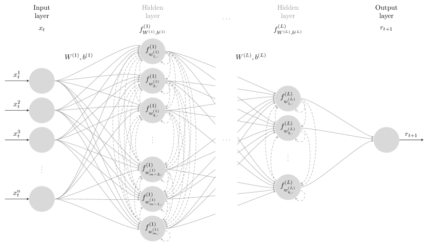
2.2.4   Estimation, Hyperparameters, Details

Due to the high dimensionality and non-linearity of the problem, estimation of a deep neural network is a complex task. Here, we provide a detailed summary of the model architectures and their estimations. We work with a variety of deep learning structures and compare them with a recurrent LSTM network and regularized OLS. We consider NN1, NN2 and NN3 models that contain 16, 32–16 and 32–16–8 neurons in the one, two, and three hidden layer structures, respectively, and an LSTM model which is a NN with 3 recurrent layers with 32-16-8 neurons in each and LSTM cells introduced into the last layer.

To prevent the model from over-fitting and to the reduce large number of parameters, we use dropout, which is a common form of regularization that has generally better performance in comparison to traditional $l_{1}$ or $l_{2}$ regularization. The term dropout refers to dropping out units in neural networks and can be shown to be a form of ridge regularization. To fit the networks, we adopt a popular and robust adaptive moment estimation algorithm (Adam) with weight decay regularization introduced by Kingma and Ba, (2014) and we use the Huber loss function in the estimation.

Further, we follow the most common approach in the literature and select tuning parameters adaptively from the data in a validation sample. We split the data into training and validation samples that maintain temporal ordering of the data and tune hyperparameters with respect to the statistical and economic criteria. We search the optimal models in the following grid of 100 randomly chosen combinations of the following hyperparameters: learning rate $\in[0.001,0.02]$, decay regularization $\in[0,0.001]$, dropout $\in[0\%,60\%]$ of weights and activation function $\in\{\text{sigmoid},\text{ReLU}\}$ with 1000 epochs with early stopping. Since the sample at each window is rather small, and final models can depend on initial values in the optimization, we use ensemble averaging of five models with randomly chosen initial values.

2.3 Optimal Portfolios

We consider a portfolio choice problem of an agent with the investment horizon of $T$ periods in the future who maximizes her expected utility over the cumulative portfolio return. There are two assets: a one-period Treasury bill and a stock index. If $\omega_{t+\tau}$ is the allocation to the stock index at time $t+\tau,$ the investor solves the following optimization problem at time $t$

$$\max_{\omega}\mathbb{E}_{t}\left[U(r_{p,t+T})\right]$$ (8)

in which the end-of-horizon portfolio return $r_{p,t+T}$ is defined as

$$r_{p,t+T}=\prod_{\tau=1}^{T}\left[(1-\omega_{t+\tau-1})\exp(r_{t+\tau}^{f})+\omega_{t+\tau-1}\exp(r_{t+\tau}^{f}+r_{t+\tau})\right],$$ (9)

and $r_{t+\tau}^{f}$ denotes a zero-coupon default-free log bond yield between $t+\tau-1$ and $t+\tau$. Following Johannes et al., (2014), we consider various choices of horizons $T$ to assess the impact of the length of the investment period. Specifically, we report the results for the two cases of six months $(T=6)$ and two years $(T=24).$ Furthermore, we allow the investor to rebalance portfolio weights with different frequencies. The allocations between a Treasury bill and a stock index are updated every three months, or once per year for the shorter or longer investment horizons, respectively. These choices of horizons and rebalancing periods allow us to compare two investment strategies. The former reflects a more actively managed portfolio with frequent changes in the allocations, whereas the latter corresponds to a relatively passive investment portfolio with less frequent rebalancing. We further winsorize the weights for the stock index to $-1\leq\omega_{t+\tau}\leq 2$ to prevent extreme investments. In the sensitivity analysis, we check the robustness of our results to alternative assumptions about the portfolio weights, particularly incorporating the borrowing and short-selling constraints.

We also assume a power utility investor

$$U(r_{p,t+\tau})=\frac{r_{p,t+\tau}^{1-\gamma}}{1-\gamma},$$

where $\gamma$ is the coefficient of risk aversion. The expected utility is defined by the predictive distribution of cumulative portfolio returns $r_{p,t+\tau}$ given by Eq.(9), which in turn depends on the corresponding model used to predict future excess returns $r_{t+\tau}$ and the law of motion of predictor variables $\mbox{\boldmath$x$}_{t}.$ For $\mbox{\boldmath$x$}_{t},$ we adopt a parsimonious AR(1) framework, that is, each variable $\mbox{\boldmath$x$}_{t}^{i}$ satisfies

$$\mbox{\boldmath$x$}_{t}^{i}=\mbox{\boldmath$\alpha$}^{x^{i}}+\mbox{\boldmath$\beta$}^{x^{i}}\mbox{\boldmath$x$}_{t-1}^{i}+\varepsilon_{t}^{x^{i}}.$$

where $\mbox{\boldmath$\alpha$}^{x^{i}}$ and $\mbox{\boldmath$\beta$}^{x^{i}}$ are coefficients, and $\varepsilon_{t}^{x^{i}}$ are normal error terms. To proxy for the joint variance-covariance matrix of the error terms $\varepsilon_{t}=(\varepsilon_{t}^{r},\varepsilon_{t}^{x}),$ we employ a sample variance estimator $\hat{\Sigma}_{t}=\hat{\varepsilon}_{t}\hat{\varepsilon}_{t}^{{}^{\prime}},$ where $\varepsilon_{t}$ are forecast errors. Finally, we set the risk aversion parameter $\gamma=4$ to compare our results to the existing literature (Johannes et al.,, 2014; Rossi,, 2018).

In sum, the investor maximizes her expected utility and optimally rebalances her portfolio weights quarterly or annually for investment horizons of six months and two years, respectively. To compute her expected utility, she uses the distribution of returns predicted by the linear regressions or the neural networks. To evaluate the impact of the investor’s conditioning information, we consider different assumptions about the set of predictors and sample periods used to estimate the models. In particular, we consider the following specifications:

• The no-predictability expectations hypothesis (EH) framework assumes a constant mean and constant variance framework with no predictors in Eq.(1), that is, $\mbox{\boldmath$\beta$}=0.$

• A simple linear regression of excess log returns with the dividend yield as a single predictor and a “kitchen sink” linear regression with all available variables. For each of the two cases, we further implement OLS regressions using all data up to time $t$ or over a 10-year rolling window, as in Johannes et al., (2014). The univariate models with the expanding and rolling windows are denoted OLS1 and OLS2, and the multivariate versions are OLS3 and OLS4.

• A set of machine learning architectures including neural networks with 1 layer of 16 neurons (NN1), 2 layers of 32-16 neurons (NN2), 3 layers of 32-16-8 neurons (NN3) and an LSTM model with 3 recurrent layers and 32-16-8 neurons and LSTM cells introduced in the last layer. All NNs use a “kitchen sink” approach by utilizing all available data to predict log excess returns and are trained on a 10-year rolling window to account for a time-varying relationship between the predictors and returns.

There are many dimensions that can be used to generalize our modelling approach. More general specifications could add additional predictor variables (McCracken and Ng,, 2016), parameter uncertainty (Wachter and Warusawitharana,, 2009; Johannes et al.,, 2014; Bianchi and Tamoni,, 2020), economic restrictions (Van Binsbergen and Koijen,, 2010), or consider a larger set of investable assests and alternative preferences (Dangl and Weissensteiner,, 2020) among other extensions. Most notably, modelling stochastic volatility via a parsimonious mean-reverting process (Johannes et al.,, 2014) or more complex GARCH- and MIDAS-type volatility estimators (Rossi,, 2018) would certainly improve the performance of our strategies. Instead, we consider all specifications with a constant volatility setting to solely evaluate the impact of neural networks on the performance of dynamic allocation strategies. Our aim is to demonstrate out-of-sample portfolio gains from using deep learning in the most restrictive setting.

2.4 Performance Evaluation

In our analysis, we employ a number of metrics measuring the statistical accuracy of the methods considered and their economic gains for the investor. With respect to the statistical performance, we first consider a common measure of mean squared prediction error (MSPE) defined as

$$MSPE=\frac{1}{T_{0}-t_{0}+1}\sum_{t=t_{0}}^{T_{0}}\Big{(}r_{t}-\hat{r}_{t}^{\mathcal{M}_{s}}\Big{)}^{2},$$ (10)

where $r_{t}$ denotes the observed excess log return, $\hat{r}_{t}^{\mathcal{M}_{s}}$ is the return predicted by a particular framework $\mathcal{M}_{s},$ and $t_{0}$ and $T_{0}$ are the months of the first and last predictions. Notice that the investor rebalances her allocations at varying frequency. Thus, we compute the prediction errors only in those periods when she reoptimizes her portfolio.

As in Campbell and Thompson, (2008), we compute the out-of-sample predictive $R^{2}_{oos}$

$$R^{2}_{oos}=1-\frac{\sum_{t=t_{0}}^{T_{0}}\big{(}r_{t}-\hat{r}_{t}^{\mathcal{M}_{s}}\big{)}^{2}}{\sum_{t=t_{0}}^{T_{0}}\big{(}r_{t}-\bar{r}_{t}\big{)}^{2}},$$

where $\bar{r}_{t}$ is the historical mean of returns. By construction, the $R_{oos}^{2}$ statistic compares the out-of-sample performance of the chosen model $\mathcal{M}_{s}$ relative to the historical average forecast. Notice that we compute the historical mean over the same sample used to estimate $\mathcal{M}_{s},$ which corresponds to either an expanding sample or a 10-year rolling window. The positive value of $R^{2}_{oos}$ indicates that the model-implied forecast has smaller mean squared predictive error compared to the error implied by the historical average forecast. Thus, we perform a formal test of the null hypothesis $R^{2}_{oos}\leq 0$ against the alternative hypothesis $R^{2}_{oos}>0$ by implementing the MSPE-adjusted Clark and West, (2007) test. Note that we calculate the Clark and West, (2007) test only if $R^{2}_{oos}$ is positive.

After we compare different models in terms of the statistical accuracy of their predictions, we assess whether superior statistical fit translates into economic gains. It is worth noting that this relationship is non-trivial. Indeed, Campbell and Thompson, (2008) and Rapach et al., (2010) note that seemingly small improvements in $R_{oos}^{2}$ could generate large benefits in practice. We start our investigation of the size of the improvements by calculating the average Sharpe ratio of portfolio returns as a common measure of portfolio performance used in finance. The drawback of this metric is that it does not take tail behaviour into account. Consequently, we follow Fleming et al., (2001) and compute the certainty equivalent return (CER) by equating the utility from CER to the average utility implied by an alternative model. Finally, we visualize the performance of all specifications by plotting the cumulative log portfolio returns over the sample period considered. This allows us to clearly see the time intervals in which the investor benefits the most from using different frameworks.

To evaluate the statistical significance of portfolio gains, we follow Bianchi et al., (2020) and implement the test á la Diebold and Mariano, (2002) . Specifically, we perform a pairwise comparison between the CERs generated by each framework under consideration and those yielded by the EH specification. For each model $\mathcal{M}_{s},$ we estimate the regression

$$\mathcal{U}_{t+T}^{\mathcal{M}_{s}}-\mathcal{U}_{t+T}^{EH}=\alpha^{\mathcal{M}_{s}}+\varepsilon_{t+T},$$

where $\mathcal{U}_{t+T}^{X}=\frac{\left(r_{p,t+T}^{X}\right)^{1-\gamma}}{1-\gamma}$ and $r_{p,t+T}^{X}$ is the cumulative portfolio return with the horizon $T.$ Testing for the difference in the CERs boils down to a test for the significance in $\alpha^{\mathcal{M}_{s}}.$

3 Empirical Results

3.1 Data and preliminary results

Our empirical analysis of the S&P 500 excess return predictability is based on the applications of a variety of linear models and non-linear machine learning methods as discussed in Section 2.3. We use a set of economic predictor variables considered by Goyal and Welch, (2008) to make our results directly comparable to the literature. Specifically, we focus on the monthly historical data of twelve predictors including dividend yield, log earning price ratio, dividend payout ratio, book to market ratio, net equity expansion, treasury bill rates, term spread, default yield spread, default return spread, cross-sectional premium, inflation growth, and monthly stock variance.

Table 1 reports the statistical accuracy of the models considered. Panels A and B show the MSPEs and $R_{oos}^{2}$ based on those periods when quarterly and annual rebalancing is occurring. As shown in Panel A, all linear regressions generate larger MSPEs compared to the constant mean and constant volatility model, while neural networks provide the best fit with the data.

Table 1: Statistical Accuracy of Excess Return Forecasts

This table reports the mean squared prediction error and out-of-sample $R^{2}_{oos}$ obtained from using different methodologies to predict future S&P 500 excess returns as outlined in Section 2.3. We compute the out-of-sample $R^{2}_{oos}$ in comparison to the expectations hypothesis using the historical mean to predict returns. Panel A shows the results when the investor maximizes a 6-month portfolio return and changes the allocations quarterly. Panel B demonstrates the results for a 2-year horizon and annual rebalancing. We compute statistical accuracy measures in those periods when the investor reevaluates her allocations with quarterly or annual frequency. We also report a p-value (in parentheses) of the null hypothesis $R^{2}_{oos}\leq 0$ following Clark and West, (2007). We report statistical significance only if $R^{2}_{oos}$ is positive. The forecast starts in February 1955. The sample period spans from January 1945 to December 2018.

	EH	OLS1	OLS2	OLS3	OLS4	NN1	NN2	NN3	LSTM
Panel A: 6-month horizon and quarterly rebalancing
MSPE$\times 10^{4}$	17.4	18.0	18.2	18.9	18.0	16.3	16.6	16.6	17.3
$R^{2}_{oos}$	0.5%	-2.5%	-3.6%	-8.0%	-2.5%	7.1%	5.1%	5.6%	1.6%
p-value	(0.152)					(0.006)	(0.007)	(0.002)	(0.002)
Panel B: 2-year horizon and annual rebalancing
MSPE$\times 10^{4}$	14.2	15.0	14.7	16.7	19.9	12.2	11.1	11.9	12.1
$R^{2}_{oos}$	2.2%	-2.8%	-0.8%	-15.0%	-36.9%	16.0%	23.8%	17.6%	17.2%
p-value	(0.171)					(0.001)	(0.014)	(0.007)	(0.008)

A multivariate linear regression does not necessarily outperform a univariate model. Indeed, a linear regression estimated on the rolling window (OLS3) is noisier and generates a larger MSPE than regressions using only dividend yield (OLS1), whereas the “kitchen sink” linear regression with an expanding window estimation (OLS4) slightly outperforms a single predictor model (OLS2). Furthermore, consistent with Goyal and Welch, (2008), none of the linear regressions can beat the simple historical mean, as indicated by the negative $R_{oos}^{2}.$ In contrast, we find that deep learning methods achieve the positive $R_{oos}^{2},$ indicating the statistical benefits of accounting for the nonlinear relationship between stock market returns and predictors, similarly to Feng et al., (2018) and Rossi, (2018). A formal test confirms that expected return predictability generated by NNs is statistically different from a naive historical mean forecast. In unreported results, we verify that the performance of all machine learning methods is statistically the same. Panel B also shows the results in favor of NNs in a setting with less frequent rebalancing.

3.2 Portfolio Results

Table 2 provides a summary of annualized CERs and monthly SRs of portfolio returns for each model assuming a 6-month (Panel A) and 2-year (Panel B) investment horizon. The summary statistics in each panel are computed for the whole sample and for recession and expansion periods as defined by the NBER recession indicator. The risk aversion parameter is $\gamma=4$.

For traditional methods, we recover a standard result: linear regressions do not generate out-of-sample improvements as measured by the CERs compared to the constant mean and constant volatility model. In terms of model-generated SRs, linear models perform slightly better than the expectations hypothesis model, with higher Sharpe ratios in case of more predictor variables. The rolling-window estimation introduces time-varying slope coefficients and leads to modest improvements. However, ignoring the estimation risk and stochastic volatility of returns results in lower CERs relative to a constant mean and volatility specification, which is consistent with Johannes et al., (2014).

Table 2: Certainty Equivalent Returns and Sharpe Ratios

This table reports the annualized certainty equivalent returns and monthly Sharpe ratios for different models outlined in Section 2.3. Panel A shows the results when the investor maximizes a 6-month portfolio return and changes the allocations quarterly. Panel B shows the results for a 2-year horizon and annual rebalancing. Each panel computes the statistics for the whole sample, with expansion and recession periods as defined by NBER. For the statistical significance of CERs, we report a one-sided p-value (in parentheses) of the test á la Diebold and Mariano, (2002). In particular, we regress the difference in utilities for each model $\mathcal{M}_{s}$ and EH: $\mathcal{U}_{t+T}^{\mathcal{M}_{s}}-\mathcal{U}_{t+T}^{EH}=\alpha^{\mathcal{M}_{s}}+\varepsilon_{t+T},$ where $\mathcal{U}_{t+T}^{X}=\frac{\left(r_{p,t+T}^{X}\right)^{1-\gamma}}{1-\gamma}$ and $r_{p,t+T}^{X}$ is the cumulative portfolio return with the horizon $T.$ Testing for the difference in the CERs boils down to a test for the significance in $\alpha^{\mathcal{M}_{s}}.$ We flag in bold font CER values that are significant at the 10% confidence level. The portfolio construction starts in February 1955. The sample period spans from January 1945 to December 2018.

	EH	OLS1	OLS2	OLS3	OLS4	NN1	NN2	NN3	LSTM
Panel A: 6-month horizon and quarterly rebalancing
1955-2018
CER	4.737	2.643	-0.030	2.781	2.491	7.295	6.984	5.491	10.007
p-value		(1.000)	(1.000)	(0.935)	(0.954)	(0.027)	(0.032)	(0.292)	(0.000)
SR	0.049	0.046	0.062	0.088	0.095	0.166	0.157	0.144	0.175
Expansions
CER	4.948	3.073	-0.173	4.598	2.045	5.873	5.280	5.304	7.998
p-value		(0.998)	(1.000)	(0.654)	(0.982)	(0.258)	(0.398)	(0.403)	(0.000)
SR	0.100	0.077	0.048	0.092	0.108	0.149	0.143	0.135	0.149
Recessions
CER	3.311	-0.274	1.401	-9.079	6.752	19.024	20.806	6.936	26.770
p-value		(0.995)	(0.648)	(0.944)	(0.221)	(0.000)	(0.000)	(0.200)	(0.000)
SR	-0.193	-0.182	0.154	0.091	0.036	0.284	0.255	0.204	0.358
Panel B: 2-year horizon and annual rebalancing
1955-2018
CER	4.542	1.068	0.040	0.923	-0.067	6.342	6.879	6.437	5.622
p-value		(1.000)	(1.000)	(0.999)	(0.997)	(0.000)	(0.000)	(0.000)	(0.012)
SR	0.048	0.044	0.046	0.083	0.081	0.138	0.136	0.129	0.118
Expansions
CER	4.448	0.826	0.514	0.321	0.231	6.051	6.390	5.913	5.537
p-value		(1.000)	(1.000)	(0.999)	(0.987)	(0.002)	(0.000)	(0.000)	(0.011)
SR	0.100	0.076	0.037	0.097	0.137	0.136	0.149	0.132	0.112
Recessions
CER	5.235	2.866	-2.924	5.930	-2.138	8.611	10.975	10.836	6.353
p-value		(0.997)	(1.000)	(0.262)	(1.000)	(0.006)	(0.000)	(0.000)	(0.284)
SR	-0.190	-0.170	0.102	0.017	-0.104	0.160	0.111	0.149	0.154

Turning to NNs, we observe that the improved $R_{oos}^{2}$ obtained using machine learning methods directly translate into economic gains for an investor. Specifically, the best-performing NN – the LSTM model – generates more than two- and three-fold increases in the annual CER (around 10% vs 4.7%) and monthly SR (0.175 vs 0.049) relative to the model ignoring expected return predictability. The LSTM model, which is a three-layer network, is directly comparable to NN3 in terms of its structure complexity. Nevertheless, LSTM dominates a standard network, emphasizing the importance of learning complex long-term temporal dynamics in addition to non-linear predictive relationships. In general, comparing NN1 through NN3, we observe that increasing the complexity of NNs does not necessarily improve portfolio performance, although all machine learning structures remain statistically equivalent to each other. A formal one-sided test confirms that, except for NN3, the portfolio performance of NNs is significantly better than the performance generated by the EH model. Further, a comparison of the results in Panels A and B demonstrates that the investor benefits more from using NNs when she manages her portfolio more actively. Overall, these results indicate that expected return predictability generated by applying nonlinear methods provides valuable information for portfolio construction.

We dissect this superior performance by looking at portfolio return statistics in periods of expansion and recession. Table 2 shows that economic gains generated by NNs are large during both regimes and are especially pronounced in recessions. For instance, the annualized CER generated by the LSTM is, on average, around 8% in good times, which is more than the 5% predicted by the EH model. In bad times, the difference in performance is extremely large, with around 26% and 3% CERs in the LSTM and EH models, respectively. A pairwise test confirms that the improvement of LSTM over EH is statistically significant during both expansions and recessions. In contrast, the portfolio returns of NN1 through NN3 are indistinguishable from EH in expansions, while shallower networks exhibit significantly better performance in recessions.

The investor who ignores expected return predictability experiences, on average, around -19% Sharpe ratios in recessions. In contrast, the LSTM model helps generate significant portfolio gains around 36% SRs, with other NNs generating at least 20% SRs on a monthly basis. Further, all NNs outperform linear regressions across good and bad times. The existing evidence for equities (Rapach et al.,, 2010; Dangl and Halling,, 2012) indicates that return predictability is concentrated in bad times. Our findings extend the existing literature by showing that, unlike linear models, NNs help the investor to effectively convert predictive variation in stock market returns into substantial economic gains across different business cycle conditions.

Table 3: Portfolio Return Statistics

This table reports mean, standard deviation, skewness, and kurtosis of optimal portfolio returns for different models as outlined in Section 2.3. All statistics are expressed in monthly terms. Panel A shows the results for the case when the investor maximizes a 6-month portfolio return and changes the allocations quarterly. Panel B shows the results for a 2-year horizon and annual rebalancing. The portfolio construction starts in February 1955. The sample period spans from January 1945 to December 2018.

	EH	OLS1	OLS2	OLS3	OLS4	NN1	NN2	NN3	LSTM
Panel A: 6-month horizon and quarterly rebalancing
Mean	0.937	2.213	4.138	4.676	6.762	10.728	9.605	9.533	11.715
St.dev.	5.504	13.871	19.122	15.353	20.502	18.601	17.641	19.121	19.343
Skew	-0.472	-0.615	-0.893	-0.332	-0.881	-0.844	-0.816	-0.786	-0.046
Kurt	4.353	8.609	10.400	7.631	9.182	11.707	12.237	11.172	4.860
Panel B: 2-year horizon and annual rebalancing
Mean	0.978	2.184	3.058	5.093	4.908	7.333	5.634	4.445	7.722
St.dev.	5.849	14.443	19.189	17.655	17.512	15.331	11.937	9.916	18.87
Skew	-0.452	-0.492	-1.058	-0.989	-0.787	-0.275	0.469	0.799	-0.013
Kurt	4.386	7.104	10.566	13.550	10.737	9.113	10.416	14.775	6.433

Table 3 presents additional statistics of portfolio returns for different methodologies. The models using NNs generate out-of-sample returns with significantly larger means. Intuitively, this occurs because machine learning methods specifically excel in risk premium prediction, that is, the conditional expectation of returns. The linear regressions and vanilla NNs do not take the time-varying volatility of returns into account and hence these models predict negative skewness and excess kurtosis (since they ignore a fat-tailed return distribution). Interestingly, although an LSTM network does not consider time variation in return volatility, it is able to identify the periods of high return variance using the long-term memory of its cells (including realized return variance as one of the predictors also helps). This results in better skewness and lower excess kurtosis. The statistics for the longer horizon portfolio are improved for the standard neural networks, where properties remain largely the same or slightly deteriorate for other models.

Figure 3: Cumulative Returns

This figure illustrates the cumulative log returns of optimal portfolio strategies from different models outlined in Section 2.3. The left panel shows the results when the investor maximizes a 6-month portfolio return and changes the allocations quarterly. The right panel shows the results for a 2-year horizon and annual rebalancing. The shaded areas denote recession periods as defined by NBER. The portfolio construction starts in February 1955. The sample period spans from January 1945 to December 2018.

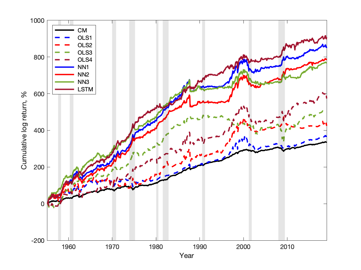
(a) 6-month horizon and quarterly rebalancing

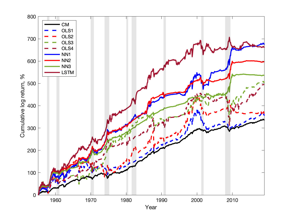
(b) 2-year horizon and annual rebalancing

We visually summarize the previous results in Figure 3, which shows the cumulative sum of log portfolio returns. The left panel shows that NNs outperform other models by a large margin. The LSTM dominates remaining networks by the end of the period considered, with a particularly pronounced difference in the second half of the sample. In relation to specific historical events, all NNs produce steady positive portfolio performance during the 2007-2008 Financial Crisis. Interestingly, the LSTM network additionally avoids a largely unexpected stock market crash, Black Monday, on October 19, 1987. Figure 3 also shows that weaker statistical performances for the passive strategy with annual rebalancing leads to lower cumulative returns across all models.

4 Further Analysis

This section dissects the performance of portfolio returns constructed in the previous section across seven decades in the post-WWII period considered. Further, this section connects economic gains of the best-performing model to common drivers of asset prices. Finally, it also provides the robustness of our conclusions to alternative measures of portfolio performance, transaction costs, borrowing and short-selling constraints, and a larger size of a rolliing window used to train NNs.

4.1 Subsample Analysis

We start by examining whether superior portfolio performance implied by NNs varies over subsamples other than expansions and recessions. Table 4 shows the certainty equivalent yields and Sharpe ratios computed separately for each decade in our sample. For the CERs, we extend the main finding of the paper: NNs, particularly LSTM, outperform the expectations hypothesis model in most cases. Specifically, the table shows that, except for the last decade, the LSTM network generates certainty equivalent values above those implied by no predictability framework. Interestingly, the formal test indicates that the improvement of LSTM over EH is significant during the first three decades, while higher CERs in later periods are statistically equivalent to those from the EH model.

The linear models perform well across the 1990s and 2010s during which the stock market grew steadily. Also, the rolling-window linear regressions tend to perform better than those using the expanding-window estimation, emphasizing the role of time-varying betas and changing information sets. For instance, Goyal and Welch, (2008) show that dividend-yield exhibited a strong predictive power for stock market returns from 1970 to mid-1990, with a weaker but mostly positive out-of-sample performance during the first two decades after World War II. In contrast, it produced large prediction errors during the 1995-2000 and 2000s. As a result, Table 4 shows that the OLS3 model generates high CERs from 1955 to 1989, exhibiting statistically better performance than EH in some case, but the model is weaker in later years when the forecast based on dividend yield had strong underperformance.

Table 4: Portfolio Performance across Subsamples

This table reports the annualized certainty equivalent returns and monthly Sharpe ratios for different models outlined in Section 2.3. The table shows the results when the investor maximizes a 6-month portfolio return and changes the allocations quarterly. The table computes the statistics for each of the seven decades since WWII. For the statistical significance of CERs, we report a one-sided p-value (in parentheses) of the test á la Diebold and Mariano, (2002). In particular, we regress the difference in utilities for each model $\mathcal{M}_{s}$ and EH: $\mathcal{U}_{t+T}^{\mathcal{M}_{s}}-\mathcal{U}_{t+T}^{EH}=\alpha^{\mathcal{M}_{s}}+\varepsilon_{t+T},$ where $\mathcal{U}_{t+T}^{X}=\frac{\left(r_{p,t+T}^{X}\right)^{1-\gamma}}{1-\gamma}$ and $r_{p,t+T}^{X}$ is the cumulative portfolio return with the horizon $T.$ Testing for the difference in the CERs boils down to a test for the significance in $\alpha^{\mathcal{M}_{s}}.$ We flag in bold font CER values that are significant at the 10% confidence level. The portfolio construction starts in February 1955. The sample period spans from January 1945 to December 2018.

	EH	OLS1	OLS2	OLS3	OLS4	NN1	NN2	NN3	LSTM
1955-1959
CER	5.467	4.376	3.219	9.495	5.545	15.611	12.220	23.120	15.455
p-value		(0.631)	(0.707)	(0.149)	(0.490)	(0.000)	(0.017)	(0.000)	(0.001)
SR	0.225	0.188	0.209	0.258	0.154	0.319	0.278	0.431	0.341
1960-1969
CER	4.197	0.580	-4.193	8.354	0.619	7.498	7.608	5.627	14.015
p-value		(0.959)	(0.991)	(0.024)	(0.931)	(0.094)	(0.042)	(0.360)	(0.000)
SR	0.062	0.064	0.030	0.157	0.067	0.164	0.148	0.181	0.241
1970-1979
CER	3.312	0.599	0.223	9.275	8.580	17.750	15.690	13.618	20.658
p-value		(1.000)	(0.847)	(0.015)	(0.026)	(0.000)	(0.000)	(0.000)	(0.000)
SR	-0.107	-0.097	0.005	0.149	0.180	0.274	0.248	0.224	0.309
1980-1989
CER	9.215	7.243	-3.130	11.276	-1.450	3.315	1.216	2.603	10.241
p-value		(0.992)	(0.983)	(0.148)	(0.969)	(0.820)	(0.906)	(0.864)	(0.282)
SR	0.048	-0.005	0.072	0.139	0.055	0.166	0.123	0.142	0.112
1990-1999
CER	8.101	11.808	13.704	-4.393	12.085	10.817	10.301	6.429	9.815
p-value		(0.002)	(0.002)	(1.000)	(0.039)	(0.052)	(0.099)	(0.842)	(0.202)
SR	0.222	0.185	0.219	-0.168	0.218	0.168	0.172	0.100	0.150
2000-2009
CER	0.000	-7.445	-7.091	-15.834	-10.520	-3.889	-0.205	-7.991	1.726
p-value		(1.000)	(0.990)	(0.998)	(0.998)	(0.869)	(0.531)	(0.995)	(0.238)
SR	-0.091	-0.125	-0.055	-0.039	-0.040	0.028	0.060	-0.062	0.084
2010-2018
CER	4.230	6.268	0.997	9.757	9.508	6.642	5.690	7.241	2.074
p-value		(0.000)	(0.999)	(0.000)	(0.000)	(0.004)	(0.049)	(0.023)	(0.842)
SR	0.237	0.220	-0.020	0.255	0.161	0.150	0.175	0.213	0.096

Turning to the SRs, NNs provide the investor with substantially higher Sharpe ratios with the exception of the 1990s and 2010s when they perform slightly worse. These results are consistent with our previous findings. Indeed, the U.S. stock market was strongly bullish in these two decades, which are marked by prolonged stock market expansions. In contrast, the Black Monday crash occurred in 1987 and the S&P 500 index recovered slowly, only by the end of the 1980s. Further, the beginning of the new millennium experienced two major crashes driven by the burst of the dot-com bubble and the subprime mortgage crisis. Table 4 shows that NNs perform significantly better than other specifications during decades with major stock bear markets and provide statistically equal results during bull markets, which is consistent with our previous results across expansions and recessions.

4.2 Drivers of Portfolio Performance

This section explores the link between the economic gains implied by the best-performing machine learning framework and prominent drivers of asset prices. In particular, we focus on the portfolio choice problem of the investor with a 6-month investment horizon and quarterly rebalancing who uses the LSTM to forecast future stock market returns. Formally, we establish this link by running a set of univariate regressions of the investor’s utility from future portfolio returns on the set of structural determinants of risk premia.

Our choice of variables is motivated by existing studies. For instance, a large strand of the literature (see Buraschi and Jiltsov, (2007) and Dumas et al., (2009) among others) emphasizes the importance of disagreement for asset prices. In our analysis, we employ the Survey of Professional Forecasters to proxy for real disagreement ($DiB(g)$) and nominal disagreement ($DiB(\pi)$), which are constructed as the interquartile range of 6-month-ahead forecasts of GDP and CPI growth. Motivated by the well-established link between asset prices and uncertainty, we employ a novel measure of economic uncertainty ($UNbex$) constructed from financial variables at high frequencies (Bekaert et al.,, 2019).

Table 5: Drivers of Portfolio Performance

This table reports the regression estimates, Newey-West p-values (in parentheses) and $R^{2}$ of economic gains on a set of selected variables determining risk premia. Economic gains are computed for portfolio returns for the best performing model employing the LSTM prediction of stock market returns. The independent variables proxy for real disagreement $DiB(g),$ nominal disagreement $DiB(\pi),$ economic uncertainty $UNbex,$ risk aversion via consumption growth $-Surplus$ or financial variables $RAbex,$ the VIX index $VIX,$ and realized stock market volatility $\sigma.$ The variables on the left and right sides are standardized. We flag in bold font regression estimates that are significant at the 10% confidence level.

	$DiB(g)$	$DiB(\pi)$	$UNbex$	$-Surplus$	$RAbex$	$VIX$	$\sigma$	$R^{2}(\%)$
(i)	0.198							3.907
	(0.002)
(ii)		0.188						3.523
		(0.019)
(iii)			0.115					1.318
			(0.127)
(iv)				0.037				0.141
				(0.561)
(v)					0.098			0.962
					(0.144)
(vi)						0.104		1.084
						(0.177)
(vii)							0.004	0.002
							(0.908)

We next examine the relationship between portfolio gains and time-varying risk aversion of investors. Following Wachter, (2006), we approximate risk aversion via the negative weighted average of consumption growth rates over a moving window of 10 years ($-Surplus$). We compare the results to an alternative measure of risk aversion extracted from financial variables (Bekaert et al.,, 2019). Finally, we relate portfolio utilities to stock market volatility by using the risk-neutral volatility ($VIX$) as measured by the VIX index and by using the realized volatility ($\sigma$) as measured by the root of the intra-month sum of squared daily S&P500 returns.

Table 5 presents the regression results. Overall, the relationship between future realized portfolio gains and most structural risk factors is rather weak. Indeed, we document that only dispersion in beliefs about a real or nominal growth is positively and statistically significantly linked to the investor’s utilities. Intuitively, this result is expected since machine learning methods significantly outperform competing models during recessionary periods, when uncertainty and disagreement in forecasts are large. The third panel in Table 5 further confirms this positive association between economic uncertainty and portfolio gains, however, the link is statistically weaker compared to disagreement measures. Except for realized stock market volatility, we obtain positive coefficients on the remaining risk factors.

4.3 Alternative Measures of Performance

Although certainty equivalent yields and Sharpe ratios are common measures of portfolio performance considered in the literature, the investor may use alternative statistics to evaluate their investment strategies, including maximum drawdown, maximum one-month loss, and average monthly turnover. For each model $\mathcal{M}_{s}$, we define maximum drawdown

$$\text{Max DD}=\max\limits_{t_{0}\leq t_{1}\leq t_{2}\leq T_{0}}\Big{[}\hat{r}_{t_{0}}^{t_{1},\mathcal{M}_{s}}-\hat{r}_{t_{0}}^{t_{2},\mathcal{M}_{s}}\Big{]},$$ (11)

in which $\hat{r}_{t_{0}}^{t,\mathcal{M}_{s}}$ denotes the cumulative portfolio return from time $t_{0}$ through $t,$ while $t_{0}$ and $T_{0}$ are the months of the first and last predictions. The maximum one-month loss measures the largest portfolio decline during the period considered. The average monthly turnover is defined as

$$\text{Turnover}=\frac{1}{T_{0}-t_{0}}\sum_{t=t_{0}+1}^{T_{0}}\Big{|}\omega_{t}-\omega_{t-1}\cdot\hat{r}_{t-1}^{\mathcal{M}_{s}}\Big{|},$$ (12)

where $\omega_{t-1}$ is the weight of the stock index.

Table 6 shows the results for alternative performance statistics. We first focus on actively managed portfolios with quarterly rebalancing and then move to more passive investment strategies with annual rebalancing. The maximum drawdown experienced by NN1 through NN3 is between 68% and 83% on the monthly basis. The linear models predict comparable or even larger drawdowns, whereas the constant mean and constant volatility model delivers a mild loss of around 23%. In contrast, the maximum drawdown for LSTM is around 46%, the mildest decline among the predictive models. Panel A further shows a similar picture for the maximum one-month loss of the portfolio: linear models and NNs tend to generate the worst one-period performance, while the LSTM strategy experiences a milder loss. Thus, the LSTM specification is the most successful in avoiding large losses over short- and long-term periods, even though it comes at the expense of the higher turnover.

Table 6: Drawdowns, Maximum Loss, and Turnover

This table reports alternative out-of-sample performance measures — maximum drawdown, maximum 1-month loss, and turnover — of optimal portfolio returns for different methodologies used to predict future S&P 500 excess returns as outlined in Section 2.3. All statistics are expressed in percentages. Panel A shows the results when the investor maximizes a 6-month portfolio return and changes the allocations quarterly. Panel B demonstrates the results for a 2-year horizon and annual rebalancing. The portfolio construction starts in February 1955. The sample period spans from January 1945 to December 2018.

	EH	OLS1	OLS2	OLS3	OLS4	NN1	NN2	NN3	LSTM
Panel A: 6-month horizon and quarterly rebalancing
Max DD	22.795	76.236	74.251	144.760	100.956	74.572	68.248	82.72	45.995
Max 1M Loss	7.795	33.325	57.974	31.756	57.974	57.974	57.974	57.974	35.011
Turnover	0.506	4.286	10.968	17.890	34.531	23.008	23.407	29.616	32.814
Panel B: 2-year horizon and annual rebalancing
Max DD	25.002	90.896	83.370	123.279	145.663	74.972	34.562	25.136	64.433
Max 1M Loss	8.036	29.431	57.974	57.974	38.862	34.375	24.419	25.136	35.011
Turnover	0.584	4.289	8.804	10.773	11.329	11.352	8.725	6.771	17.459

Panel B in Table 6 shows that the investor engaging in less frequent portfolio rebalancing is generally less efficient in forming the optimal portfolio if he relies on the linear regressions. Interestingly, the benefits of deep learning methods remain similar and even improve in some cases. For instance, the maximum one-month and drawdown losses tend to increase from 83% to more than 140% for the linear models, while NNs produce the largest declines, from 25% to 35% per month. Furthermore, as the portfolio weights are kept unchanged for longer investment periods, the turnover is reduced. Thus, the passive investor who is mainly interested in reducing his short- and long-term tail risks would still find NNs useful, while he does not benefit from linear predictive models.

In sum, exploiting expected return predictability via NNs for portfolio construction leads to riskier investments. It also generates increased turnover, especially for the best-performing model using the LSTM network. A natural question arises if these benefits are offset by the large transaction costs implied by more aggressive buying and selling stocks

4.4 Portfolio Performance with Transaction Costs

This subsection extends the main analysis by accounting for the effect of transaction costs. Specifically, we consider low and high transaction costs that are equal to the percentage paid by the investor for the change in value traded. Let $\tau$ denote a transaction cost parameter. Then the transaction-costs adjusted returns are defined as

$$\hat{r}_{t}^{\tau,\mathcal{M}_{s}}=\hat{r}_{t}^{\mathcal{M}_{s}}-\tau\big{|}\omega_{t}-\omega_{t-1}\cdot\hat{r}_{t-1}^{\mathcal{M}_{s}}\big{|},$$

where $\tau$ can attain one of the two possible values $\tau_{l}=0.1\%$ or $\tau_{h}=0.5\%.$

Table 7: Portfolio Performance with Transaction Costs

This table reports the annualized certainty equivalent returns and Sharpe ratios for different models outlined in Section 2.3. The top and bottom sections of the table compute optimal returns with low $(\tau=0.1\%)$ and high $(\tau=0.5\%)$ transaction costs. Panels A and C show the results when the investor maximizes a 6-month portfolio return and changes the allocations quarterly. Panel B and D show the results for a 2-year horizon and annual rebalancing. Each panel computes the statistics for the whole sample. For the statistical significance of CERs, we report a one-sided p-value (in parentheses) of the test á la Diebold and Mariano, (2002). In particular, we regress the difference in utilities for each model $\mathcal{M}_{s}$ and EH:$\mathcal{U}_{t+T}^{\mathcal{M}_{s}}-\mathcal{U}_{t+T}^{EH}=\alpha^{\mathcal{M}_{s}}+\varepsilon_{t+T},$ where $\mathcal{U}_{t+T}^{X}=\frac{\left(r_{p,t+T}^{X}\right)^{1-\gamma}}{1-\gamma}$ and $r_{p,t+T}^{X}$ is the cumulative portfolio return with the horizon $T.$ Testing for the difference in the CERs boils down to a test for the significance in $\alpha^{\mathcal{M}_{s}}.$ We flag in bold font those CER values that are significant at the 10% confidence level. The portfolio construction starts in February 1955. The sample period spans from January 1945 to December 2018.

	EH	OLS1	OLS2	OLS3	OLS4	NN1	NN2	NN3	LSTM
Low Transaction Costs
Panel A: 6-month horizon and quarterly rebalancing
CER	4.731	2.589	-0.171	2.548	2.036	6.996	6.689	5.115	9.592
p-value		(1.000)	(1.000)	(0.953)	(0.978)	(0.045)	(0.054)	(0.391)	(0.000)
SR	0.049	0.045	0.060	0.084	0.089	0.162	0.153	0.139	0.169
Panel B: 2-year horizon and annual rebalancing
CER	4.535	0.998	-0.085	0.765	-0.241	6.191	6.783	6.366	5.413
p-value		(1.000)	(1.000)	(0.999)	(0.998)	(0.001)	(0.000)	(0.000)	(0.033)
SR	0.048	0.043	0.044	0.081	0.079	0.135	0.134	0.127	0.115
High Transaction Costs
Panel C: 6-month horizon and quarterly rebalancing
CE	4.706	2.370	-0.736	1.609	0.193	5.791	5.501	3.592	7.910
p-value		(1.000)	(1.000)	(0.990)	(0.999)	(0.214)	(0.263)	(0.784)	(0.000)
SR	0.048	0.041	0.053	0.068	0.066	0.145	0.134	0.117	0.145
Panel D: 2-year horizon and annual rebalancing
CE	4.506	0.717	-0.586	0.129	-0.943	5.579	6.396	6.080	4.563
p-value		(1.000)	(1.000)	(1.000)	(0.999)	(0.022)	(0.000)	(0.000)	(0.453)
SR	0.047	0.039	0.038	0.073	0.070	0.125	0.123	0.117	0.102

Table 7 presents summary statistics of the out-of-sample portfolio returns with low (Panels A and B) and high (Panels C and D) transaction costs. The results show that: (1) portfolio performance is monotonically decreasing in terms of the percentage paid in transaction costs (2) the key findings reported in the main analysis remain the same; that is, the NNs consistently outperform the traditional linear predictive regressions and the expectations hypothesis framework by generating substantially higher CER and SR values; and (3) among the NNs considered, the LSTM architecture remains a dominant specification. Quantitatively, the annualized CERs for all NNs decline by less than 0.5% and 2.1% for the low and high transaction cost parameters, respectively. In terms of SRs, the decline in performance never exceeds 2% and 3% on a monthly basis for basic NNs and LSTM. However, despite a slightly detrimental effect of transaction costs, the best-performing models (NN1 and LSTM) with an actively managed portfolio generate more than two- and three-fold increases in the CERs and SRs compared to the scenario in which expected return predictability is ignored. The formal test shows that the CER gains are also statistically significant.

4.5 Borrowing and Short-selling Constraints

We consider an additional robustness check of the alternative assumptions about the portfolio weights. The main analysis allows the investor to borrow the money or to short-sell the stock by considering the weights in the interval $-1\leq\omega_{t}\leq 2.$ In this subsection, we perform a two-step analysis: we first impose borrowing constraints by restricting the optimal weight on the risk-free investment to be non-negative and then additionally imposing short-selling constrains with the weights $0\leq\omega_{t}\leq 1.$

Table 8 reports the results for the two scenarios. We focus on the quarterly rebalancing case reported in Panels A and C. The corresponding results for the passive portfolios, which are shown in Panels B and D, remain qualitatively similar. Several observations are noteworthy. First, winsorizing the weights to narrower intervals leads to ambiguous conclusions about the performance of linear predictive models. On the one hand, the constraints prevent optimal investments and hence lead to smaller out-of-sample Sharpe ratios. On the other hand, using the certainty equivalent as a measure of portfolio performance, the linear specifications consistently generate improved results, with the CERs above 3.5% in all cases. Thus, constraints on the optimal weights result in higher CERs. The reason for this seemingly counterintuitive result is that such restrictions prevent the expected utility from achieving unbounded large values (Johannes et al.,, 2014) and, therefore, avoid extreme investments based on unstable predictions of linear regressions (Goyal and Welch,, 2008). Since the certainty equivalent measure takes tail behaviour of returns into account, less extreme investments ultimately yield improved results.

Table 8: Portfolio Performance with Borrowing and Short-Selling Constraints

This table reports the annualized certainty equivalent returns and Sharpe ratios for different models outlined in Section 2.3. The top section of the table imposes borrowing constrains, while the bottom section additionally assumes short-selling constraints. Panels A and C show the results when the investor maximizes a 6-month portfolio return and changes the allocations quarterly. Panels B and D show the results for a 2-year horizon and annual rebalancing. For the statistical significance of CERs, we report a one-sided p-value (in parentheses) of the test á la Diebold and Mariano, (2002). In particular, we regress the difference in utilities for each model $\mathcal{M}_{s}$ and EH: $\mathcal{U}_{t+T}^{\mathcal{M}_{s}}-\mathcal{U}_{t+T}^{EH}=\alpha^{\mathcal{M}_{s}}+\varepsilon_{t+T},$ where $\mathcal{U}_{t+T}^{X}=\frac{\left(r_{p,t+T}^{X}\right)^{1-\gamma}}{1-\gamma}$ and $r_{p,t+T}^{X}$ is the cumulative portfolio return with the horizon $T.$ Testing for the difference in the CERs boils down to a test for the significance in $\alpha^{\mathcal{M}_{s}}.$ We flag in bold font CER values that are significant at the 10% confidence level. The portfolio construction starts in February 1955. The sample period spans from January 1945 to December 2018.

	EH	OLS1	OLS2	OLS3	OLS4	NN1	NN2	NN3	LSTM
Borrowing Constraint
Panel A: 6-month horizon and quarterly rebalancing
CER	4.737	3.662	3.371	4.149	4.560	9.122	7.632	6.900	8.560
p-value		(0.999)	(0.958)	(0.770)	(0.591)	(0.000)	(0.000)	(0.003)	(0.000)
SR	0.049	0.046	0.061	0.074	0.080	0.176	0.146	0.135	0.157
Panel B: 2-year horizon and annual rebalancing
CER	4.542	2.780	2.936	2.974	1.560	4.964	5.336	5.275	5.321
p-value		(1.000)	(1.000)	(1.000)	(1.000)	(0.147)	(0.007)	(0.008)	(0.033)
SR	0.048	0.044	0.051	0.049	0.013	0.101	0.094	0.087	0.100
Borrowing and Short-Selling Constraints
Panel C: 6-month horizon and quarterly rebalancing
CER	4.737	3.704	4.707	5.353	5.708	7.500	6.758	7.128	7.775
p-value		(0.998)	(0.528)	(0.080)	(0.004)	(0.000)	(0.000)	(0.000)	(0.000)
SR	0.049	0.047	0.066	0.093	0.093	0.146	0.129	0.138	0.150
Panel D: 2-year horizon and annual rebalancing
CER	4.542	2.780	3.757	4.261	5.010	5.809	5.320	5.408	6.117
p-value		(1.000)	(1.000)	(0.859)	(0.004)	(0.000)	(0.000)	(0.000)	(0.000)
SR	0.048	0.044	0.054	0.054	0.071	0.107	0.109	0.098	0.107

Second, unlike the linear regressions, we document a negative impact of imposing borrowing and short-selling constraints on portfolio performance implied by NNs. For instance, Panels A and B in Table 8 demonstrate a decline in both CERs and SRs for all NNs, with a larger drop in performance measures in response to more stringent assumptions about the weights. Nevertheless, despite weaker performance of machine learning methods, the table confirms the key results of the main analysis. Specifically, traditional predictive models barely generate a positive value for the investor, whereas there is robust statistical evidence of substantial improvements from using NNs.

4.6 Different Rolling Window Sizes

The subperiod analysis presented in Table 4 reveals a slightly declining performance of NNs by the end of the sample. In particular, the LSTM generates higher CERs than the EH model, however, the difference proves to be statistically indistinguishable over the last four decades. This raises the question whether the evidence in this paper holds for more recent data. This subsection demonstrates that the main conclusions of this paper indeed remain intact.

Table 9 reports summary statistics of the out-of-sample portfolio returns, which are obtained for the subperiod from February 1969 to December 2018 as in Rossi, (2018). In relation to the models using the rolling-window estimation, we assume a 20-year horizon to assess the impact of longer history on the performance of different methodologies, particularly machine learning methods that are assumed to work better with larger samples. Notice that the quantitative predictions of this exercise are not directly comparable to the previous results due to difference in the historical data. In particular, the period from February 1969 to December 2018 is characterized by slightly weaker market performance, which ultimately translates into a less favorable opportunity set for the investor. The returns statistics in Table 9 are consistent with this intuition. The average Sharpe ratio implied by the model with no predictability shrinks to half the size of that in the benchmark analysis. The linear models experience comparable deterioration in results.

Table 9: Portfolio Performance from Feb 1969:02 to Dec 2018: 20-year rolling window

This table reports the annualized certainty equivalent returns and Sharpe ratios for different models outlined in Section 2.3. The rolling window estimation uses 20 years of recent data. Panel A shows the results when the investor maximizes a 6-month portfolio return and changes the allocations quarterly. Panel B shows the results for a 2-year horizon and annual rebalancing. Each panel computes the statistics for the whole sample, expansion and recession periods as defined by the NBER. For the statistical significance of CERs, we report a one-sided p-value (in parentheses) of the test á la Diebold and Mariano, (2002). In particular, we regress the difference in utilities for each model $\mathcal{M}_{s}$ and EH: $\mathcal{U}_{t+T}^{\mathcal{M}_{s}}-\mathcal{U}_{t+T}^{EH}=\alpha^{\mathcal{M}_{s}}+\varepsilon_{t+T},$ where $\mathcal{U}_{t+T}^{X}=\frac{\left(r_{p,t+T}^{X}\right)^{1-\gamma}}{1-\gamma}$ and $r_{p,t+T}^{X}$ is the cumulative portfolio return with the horizon $T.$ Testing for the difference in the CERs boils down to a test for the significance in $\alpha^{\mathcal{M}_{s}}.$ We flag in bold font CER values that are significant at the 10% confidence level. The portfolio construction starts in February 1969.

	EH	OLS1	OLS2	OLS3	OLS4	NN1	NN2	NN3	LSTM
Panel A: 6-month horizon and quarterly rebalancing
1969-2018
CER	4.600	1.763	0.791	1.025	3.707	6.762	6.601	6.236	7.253
p-value		1.000	1.000	0.984	0.811	0.018	0.053	0.061	0.016
SR	0.025	0.010	0.018	0.059	0.057	0.135	0.140	0.132	0.165
Expansions
CER	5.038	3.158	2.479	4.551	5.846	7.237	7.314	5.673	6.734
p-value		0.999	0.997	0.694	0.158	0.008	0.022	0.335	0.039
SR	0.090	0.059	0.045	0.070	0.068	0.139	0.138	0.141	0.161
Recessions
CER	1.846	-6.771	-9.496	-18.688	-8.560	3.819	2.347	4.423	17.657
p-value		1.000	0.999	0.985	0.980	0.345	0.465	0.287	0.002
SR	-0.251	-0.253	-0.123	0.034	0.023	0.123	0.156	0.061	0.226
Panel B: 2-year horizon and annual rebalancing
1969-2018
CER	4.530	0.508	-2.573	-2.558	2.080	5.788	5.136	7.038	6.477
p-value		(1.000)	(1.000)	(1.000)	(1.000)	(0.026)	(0.068)	(0.000)	(0.000)
SR	0.023	0.008	-0.002	0.008	0.025	0.126	0.084	0.117	0.135
Expansions
CER	4.448	0.246	-2.160	-2.174	3.324	5.465	4.675	6.739	6.185
p-value		(1.000)	(1.000)	(1.000)	(0.992)	(0.076)	(0.297)	(0.000)	(0.001)
SR	0.089	0.059	0.035	0.008	0.021	0.108	0.054	0.100	0.127
Recessions
CER	5.089	2.275	-5.061	-4.914	-4.333	8.133	8.538	9.073	8.409
p-value		(0.999)	(1.000)	(1.000)	(1.000)	(0.023)	(0.004)	(0.003)	(0.009)
SR	-0.248	-0.259	-0.194	0.010	0.045	0.216	0.211	0.210	0.181

For NNs with quarterly rebalancing, we document several interesting observations. First, despite a weaker performance of the stock market during the period considered, monthly Sharpe ratios implied by NNs decrease marginally, with the drop approximately equal to 0.01 to 0.03 relative to the main results. Second, comparing NN1 through NN3 in terms of certainty equivalent returns, NNs yield statistically the same results. Although deeper networks generate slightly lower CERs than those predicted by shallower networks, the p-values indicate that these model-based values remain in the same equivalence class. Third, the LSTM still produces the most significant economic gains. Specifically, the annualized certainty equivalent yield is above 7% and monthly Sharpe ratios remain as high as 0.165. Finally, unlike weak statistical evidence of the main results with recent data, the formal test of the results in this subsection demonstrates strong statistical evidence in favor of NNs. The reason is that NNs use a 20-year rolling window for hyperparameter tuning, which helps them to better learn non-linear relationships, and short- and long-term dependencies (in case of LSTM) from the data.

5 Conclusion

In this paper, we evaluate the economic gains of using deep learning methods for the construction of optimal portfolios. We study the portfolio allocation of a long-horizon investor who uses neural networks to predict future returns when choosing an optimal allocation between a market portfolio and a risk-free asset. We propose and compare various architectures of neural networks including shallow and deep feedforward NNs as well as the LSTM specification, which is capable of learning the long-term relationships. Three key findings emerge from our investigation.

First, we demonstrate that sound statistical performance of non-linear machine learning methods, such as neural networks, leads to large and significant out-of-sample portfolio gains. These gains are robust to a variety of portfolio performance measures, the inclusion of transaction costs, borrowing and short-selling constraints. Second, we find that employing the forecasts of deeper networks does not necessarily translate into larger economic gains. In order to identify and benefit from a complex non-linear predictive relationship, the investor needs to harvest more data, while shallower NNs might be a better option in a setting with small samples. In terms of NNs, we further show that the novel LSTM is the best-performing specification. This emphasizes the critical role of short- and long-term order dependencies in predicting stock returns, in addition to approximating the non-linear relationship. Finally, we document that NNs perform well even in the absence of additional ingredients, such as time-varying return volatility, which are commonly proposed by the literature studying linear predictive regressions. Our results show that NNs are capable of identifying these complex features from the data in a non-parametric way and without any specific modelling assumptions.

Our analysis can be extended in a number of ways. It would be interesting to examine the interaction between NNs and alternative preference specifications. In particular, it is not clear whether an investor with a tail sensitive utility function or a preference for early resolution of uncertainty would be able to generate comparable economic gains. Van Binsbergen and Koijen, (2010) present evidence that additional economic restrictions can actually improve the model’s performance. Our results point out a negative impact of restricting portfolio weights on the gains of the NNs. It would be interesting to examine if our evidence holds in a setting with other restrictions, in particular those proposed by Van Binsbergen and Koijen, (2010). Finally, extending our analysis to multiple assets is a straightforward exercise, which would shed light on the economic significance of forecasting returns of different asset classes via NNs.

References

- Ang and Bekaert, (2007) Ang, A. and Bekaert, G. (2007). Stock return predictability: Is it there? The Review of Financial Studies, 20(3):651–707.
- Avramov, (2002) Avramov, D. (2002). Stock return predictability and model uncertainty. Journal of Financial Economics, 64(3):423–458.
- Baillie and Kapetanios, (2007) Baillie, R. T. and Kapetanios, G. (2007). Testing for neglected nonlinearity in long-memory models. Journal of Business & Economic Statistics, 25(4):447–461.
- Barberis, (2000) Barberis, N. (2000). Investing for the long run when returns are predictable. The Journal of Finance, 55(1):225–264.
- Bekaert et al., (2019) Bekaert, G., Engstrom, E. C., and Xu, N. R. (2019). The time variation in risk appetite and uncertainty. Technical report, National Bureau of Economic Research.
- Bianchi et al., (2020) Bianchi, D., Büchner, M., and Tamoni, A. (2020). Bond risk premia with machine learning. Review of Financial Studies, (forthcoming).
- Bianchi and Tamoni, (2020) Bianchi, D. and Tamoni, A. (2020). Sparse predictive regressions: Statistical performance and economic significance. Machine Learning for Asset Management: New Developments and Financial Applications, pages 75–113.
- Breiman et al., (2001) Breiman, L. et al. (2001). Statistical modeling: The two cultures (with comments and a rejoinder by the author). Statistical science, 16(3):199–231.
- Bryzgalova et al., (2019) Bryzgalova, S., Pelger, M., and Zhu, J. (2019). Forest through the trees: Building cross-sections of stock returns. Available at SSRN 3493458.
- Buraschi and Jiltsov, (2007) Buraschi, A. and Jiltsov, A. (2007). Habit formation and macroeconomic models of the term structure of interest rates. The Journal of Finance, 62(6):3009–3063.
- Campbell, (1987) Campbell, J. Y. (1987). Stock returns and the term structure. Journal of financial economics, 18(2):373–399.
- Campbell and Shiller, (1988) Campbell, J. Y. and Shiller, R. J. (1988). The dividend-price ratio and expectations of future dividends and discount factors. The Review of Financial Studies, 1(3):195–228.
- Campbell and Thompson, (2008) Campbell, J. Y. and Thompson, S. B. (2008). Predicting excess stock returns out of sample: Can anything beat the historical average? The Review of Financial Studies, 21(4):1509–1531.
- Campbell and Yogo, (2006) Campbell, J. Y. and Yogo, M. (2006). Efficient tests of stock return predictability. Journal of financial economics, 81(1):27–60.
- Chen et al., (2019) Chen, L., Pelger, M., and Zhu, J. (2019). Deep learning in asset pricing. Available at SSRN 3350138.
- Chen et al., (2020) Chen, L., Pelger, M., and Zhu, J. (2020). Deep learning in asset pricing. Available at SSRN 3350138.
- Clark and West, (2007) Clark, T. and West, K. (2007). Approximately normal tests for equal predictive accuracy in nested models. Journal of econometrics, 138(1):291–311.
- Cochrane, (2008) Cochrane, J. H. (2008). The dog that did not bark: A defense of return predictability. The Review of Financial Studies, 21(4):1533–1575.
- Cremers, (2002) Cremers, K. M. (2002). Stock return predictability: A bayesian model selection perspective. The Review of Financial Studies, 15(4):1223–1249.
- Dangl and Halling, (2012) Dangl, T. and Halling, M. (2012). Predictive regressions with time-varying coefficients. Journal of Financial Economics, 106(1):157–181.
- Dangl and Weissensteiner, (2020) Dangl, T. and Weissensteiner, A. (2020). Optimal portfolios under time-varying investment opportunities, parameter uncertainty, and ambiguity aversion. Journal of Financial and Quantitative Analysis, 55(4):1163–1198.
- Diebold and Mariano, (2002) Diebold, F. X. and Mariano, R. S. (2002). Comparing predictive accuracy. Journal of Business & economic statistics, 20(1):134–144.
- Dumas et al., (2009) Dumas, B., Kurshev, A., and Uppal, R. (2009). Equilibrium portfolio strategies in the presence of sentiment risk and excess volatility. The Journal of Finance, 64(2):579–629.
- Fama and French, (1988) Fama, E. F. and French, K. R. (1988). Dividend yields and expected stock returns. Journal of financial economics, 22(1):3–25.
- Fama and French, (1989) Fama, E. F. and French, K. R. (1989). Business conditions and expected returns on stocks and bonds. Journal of financial economics, 25(1):23–49.
- Feng et al., (2018) Feng, G., He, J., and Polson, N. G. (2018). Deep learning for predicting asset returns. arXiv preprint arXiv:1804.09314.
- Feng et al., (2019) Feng, G., Polson, N., and Xu, J. (2019). Deep learning in characteristics-sorted factor models. Available at SSRN 3243683.
- Ferson and Harvey, (1991) Ferson, W. E. and Harvey, C. R. (1991). The variation of economic risk premiums. Journal of Political Economy, 99(2):385–415.
- Ferson et al., (2003) Ferson, W. E., Sarkissian, S., and Simin, T. T. (2003). Spurious regressions in financial economics? The Journal of Finance, 58(4):1393–1413.
- Fleming et al., (2001) Fleming, J., Kirby, C., and Ostdiek, B. (2001). The economic value of volatility timing. The Journal of Finance, 56(1):329–352.
- Freyberger et al., (2020) Freyberger, J., Neuhierl, A., and Weber, M. (2020). Dissecting characteristics nonparametrically. The Review of Financial Studies, 33(5):2326–2377.
- Fuster et al., (2018) Fuster, A., Goldsmith-Pinkham, P., Ramadorai, T., and Walther, A. (2018). Predictably unequal? the effects of machine learning on credit markets. The Effects of Machine Learning on Credit Markets (November 6, 2018).
- Gargano et al., (2019) Gargano, A., Pettenuzzo, D., and Timmermann, A. (2019). Bond return predictability: Economic value and links to the macroeconomy. Management Science, 65(2):508–540.
- Giannone et al., (2017) Giannone, D., Lenza, M., and Primiceri, G. E. (2017). Economic predictions with big data: The illusion of sparsity.
- Giglio and Xiu, (2017) Giglio, S. and Xiu, D. (2017). Inference on risk premia in the presence of omitted factors. Technical report, National Bureau of Economic Research.
- Goyal and Welch, (2008) Goyal, A. and Welch, I. (2008). A comprehensive look at the empirical performance of equity premium prediction. The Review of Financial Studies, 21(4):1455–1508.
- Green et al., (2013) Green, J., Hand, J. R., and Zhang, X. F. (2013). The supraview of return predictive signals. Review of Accounting Studies, 18(3):692–730.
- Gu et al., (2020) Gu, S., Kelly, B., and Xiu, D. (2020). Empirical asset pricing via machine learning. The Review of Financial Studies, 33(5):2223–2273.
- Harvey et al., (2016) Harvey, C. R., Liu, Y., and Zhu, H. (2016). … and the cross-section of expected returns. The Review of Financial Studies, 29(1):5–68.
- Heaton et al., (2017) Heaton, J. B., Polson, N. G., and Witte, J. H. (2017). Deep learning for finance: deep portfolios. Applied Stochastic Models in Business and Industry, 33(1):3–12.
- Henkel et al., (2011) Henkel, S. J., Martin, J. S., and Nardari, F. (2011). Time-varying short-horizon predictability. Journal of financial economics, 99(3):560–580.
- Hochreiter and Schmidhuber, (1997) Hochreiter, S. and Schmidhuber, J. (1997). Long short-term memory. Neural computation, 9(8):1735–1780.
- Hodrick, (1992) Hodrick, R. J. (1992). Dividend yields and expected stock returns: Alternative procedures for inference and measurement. The Review of Financial Studies, 5(3):357–386.
- Hutchinson et al., (1994) Hutchinson, J. M., Lo, A. W., and Poggio, T. (1994). A nonparametric approach to pricing and hedging derivative securities via learning networks. The Journal of Finance, 49(3):851–889.
- Israel et al., (2020) Israel, R., Kelly, B. T., and Moskowitz, T. J. (2020). Can machines ’learn’ finance? Available at SSRN 3624052.
- Jiang et al., (2020) Jiang, J., Kelly, B. T., and Xiu, D. (2020). (re-) imag (in) ing price trends. Chicago Booth Research Paper, (21-01).
- Johannes et al., (2014) Johannes, M., Korteweg, A., and Polson, N. (2014). Sequential learning, predictability, and optimal portfolio returns. The Journal of Finance, 69(2):611–644.
- Kelly and Pruitt, (2013) Kelly, B. and Pruitt, S. (2013). Market expectations in the cross-section of present values. The Journal of Finance, 68(5):1721–1756.
- Kelly and Pruitt, (2015) Kelly, B. and Pruitt, S. (2015). The three-pass regression filter: A new approach to forecasting using many predictors. Journal of Econometrics, 186(2):294–316.
- Kelly et al., (2019) Kelly, B. T., Pruitt, S., and Su, Y. (2019). Characteristics are covariances: A unified model of risk and return. Journal of Financial Economics, 134(3):501–524.
- Kingma and Ba, (2014) Kingma, D. P. and Ba, J. (2014). Adam: A method for stochastic optimization. arXiv preprint arXiv:1412.6980.
- Kozak et al., (2020) Kozak, S., Nagel, S., and Santosh, S. (2020). Shrinking the cross-section. Journal of Financial Economics, 135(2):271–292.
- Kuan and White, (1994) Kuan, C.-M. and White, H. (1994). Artificial neural networks: An econometric perspective. Econometric reviews, 13(1):1–91.
- Lettau and Ludvigson, (2001) Lettau, M. and Ludvigson, S. (2001). Consumption, aggregate wealth, and expected stock returns. the Journal of Finance, 56(3):815–849.
- Lettau and Van Nieuwerburgh, (2008) Lettau, M. and Van Nieuwerburgh, S. (2008). Reconciling the return predictability evidence: The review of financial studies: Reconciling the return predictability evidence. The Review of Financial Studies, 21(4):1607–1652.
- Lewellen, (2004) Lewellen, J. (2004). Predicting returns with financial ratios. Journal of Financial Economics, 74(2):209–235.
- Lopez de Prado, (2019) Lopez de Prado, M. (2019). Beyond econometrics: A roadmap towards financial machine learning. Available at SSRN 3365282.
- McCracken and Ng, (2016) McCracken, M. W. and Ng, S. (2016). Fred-md: A monthly database for macroeconomic research. Journal of Business & Economic Statistics, 34(4):574–589.
- Menzly et al., (2004) Menzly, L., Santos, T., and Veronesi, P. (2004). Understanding predictability. Journal of Political Economy, 112(1):1–47.
- Messmer, (2017) Messmer, M. (2017). Deep learning and the cross-section of expected returns. Available at SSRN 3081555.
- Pástor and Stambaugh, (2009) Pástor, L. and Stambaugh, R. F. (2009). Predictive systems: Living with imperfect predictors. The Journal of Finance, 64(4):1583–1628.
- Paye and Timmermann, (2006) Paye, B. S. and Timmermann, A. (2006). Instability of return prediction models. Journal of Empirical Finance, 13(3):274–315.
- Pesaran and Timmermann, (1995) Pesaran, M. H. and Timmermann, A. (1995). Predictability of stock returns: Robustness and economic significance. The Journal of Finance, 50(4):1201–1228.
- Racine, (2001) Racine, J. (2001). On the nonlinear predictability of stock returns using financial and economic variables. Journal of Business & Economic Statistics, 19(3):380–382.
- Rapach et al., (2010) Rapach, D., Strauss, J., and Zhou, G. (2010). Out-of-sample equity premium prediction: Combination forecasts and links to the real economy. Review of Financial Studies, 23(2):821–862.
- Rossi, (2018) Rossi, A. G. (2018). Predicting stock market returns with machine learning. Technical report, Working paper.
- Santos and Veronesi, (2006) Santos, T. and Veronesi, P. (2006). Labor income and predictable stock returns. The Review of Financial Studies, 19(1):1–44.
- Shiller, (1981) Shiller, R. (1981). Do stock prices move too much to be justified by subsequent changes in dividends? American Economic Review, 71:421–436.
- Sirignano et al., (2016) Sirignano, J., Sadhwani, A., and Giesecke, K. (2016). Deep learning for mortgage risk. arXiv preprint arXiv:1607.02470.
- Stambaugh, (1999) Stambaugh, R. F. (1999). Predictive regressions. Journal of Financial Economics, 54(3):375–421.
- Tobek and Hronec, (2020) Tobek, O. and Hronec, M. (2020). Does it pay to follow anomalies research? machine learning approach with international evidence. Journal of Financial Markets, page 100588.
- Torous et al., (2004) Torous, W., Valkanov, R., and Yan, S. (2004). On predicting stock returns with nearly integrated explanatory variables. The Journal of Business, 77(4):937–966.
- Van Binsbergen and Koijen, (2010) Van Binsbergen, J. H. and Koijen, R. S. (2010). Predictive regressions: A present-value approach. The Journal of Finance, 65(4):1439–1471.
- Wachter, (2006) Wachter, J. A. (2006). A consumption-based model of the term structure of interest rates. Journal of Financial economics, 79(2):365–399.
- Wachter and Warusawitharana, (2009) Wachter, J. A. and Warusawitharana, M. (2009). Predictable returns and asset allocation: Should a skeptical investor time the market? Journal of Econometrics, 148(2):162–178.
- Zhang et al., (2020) Zhang, Z., Zohren, S., and Roberts, S. (2020). Deep learning for portfolio optimisation. arXiv preprint arXiv:2005.13665.