Modeling protoplanetary disk SEDs with artificial neural networks

We model the spectral energy distributions (SEDs) of 23 protoplanetary disks in the Taurus-Auriga star-forming region using detailed disk models and a Bayesian approach. This is made possible by combining these models with artificial neural networks to drastically speed up their performance. Such a setup allows us to confront $\alpha$-disk models with observations while accounting for several uncertainties and degeneracies. Our results yield high viscosities and accretion rates for many sources, which is not consistent with recent measurements of low turbulence levels in disks. This inconsistency could imply that viscosity is not the main mechanism for angular momentum transport in disks, and that alternatives such as disk winds play an important role in this process. We also find that our SED-derived disk masses are systematically higher than those obtained solely from (sub)mm fluxes, suggesting that part of the disk emission could still be optically thick at (sub)mm wavelengths. This effect is particularly relevant for disk population studies and alleviates previous observational tensions between the masses of protoplanetary disks and exoplanetary systems.

1 Introduction

The field of protoplanetary disks has undergone a revolution during in recent years thanks to the improvement in sensitivity and spatial resolution of new facilities. In particular, the Atacama Large Millimeter/submillimeter Array (ALMA) has produced censuses of disk dust and gas masses in different star-forming regions (e.g., Ansdell et al. 2016; Miotello et al. 2016), revealed the ubiquity of substructures in disks (e.g., Andrews et al. 2018a; Long et al. 2018), and found evidence for low viscosities in these systems (e.g., Pinte et al. 2016; Flaherty et al. 2017; Dong et al. 2018), among other results. These new data have clearly proven that planet formation theories are still incomplete, and that some of the assumptions that are typically made require further consideration.

One important concept that has been increasingly questioned lately is the $\alpha$-disk prescription (e.g., Shakura & Sunyaev 1973), which is at the base of many models of protoplanetary disks. In this prescription, the transport of angular momentum is due to viscosity, $\nu$, which is proportional to the local sound speed $c_{s}$ and the scale height $H$ ($\nu=\alpha c_{s}H$, with $\alpha$ being constant throughout the disk, e.g., Lynden-Bell & Pringle 1974; Pringle 1981). The origin of this turbulent viscosity is usually attributed to the magneto-rotational instability (MRI, Balbus & Hawley 1991). However, theoretical studies have shown that this effect may not be sufficiently strong in protoplanetary disks: The midplane is shielded from ionizing radiation and its ionization fraction is low (Stone et al. 1998), and the effects of non-ideal magnetohydrodynamics could be enough to suppress MRI everywhere in the disk (Bai & Stone 2013). Supported by recent observational evidence of low turbulence levels, disk winds have gained increasing relevance as the potential main mechanism of angular momentum transport in disks (e.g., Bai & Stone 2013; Simon et al. 2015; Bai et al. 2016; Bai 2016).

A second paradigm shift involves disk masses and the time of planet formation. ALMA has yielded complete censuses of disk dust masses for several star-forming regions, allowing for comparative studies as a function of different factors (age, stellar mass, environment, see e.g., Ansdell et al. 2016; Miotello et al. 2016; Cieza et al. 2019; Williams et al. 2019). Among the many results derived from this wealth of data, one emerging trend is that the masses of disks between 1-3 Myr appear to be consistently lower than the masses of confirmed exoplanetary systems. This suggests that dust and gas masses could be systematically underestimated and/or that planetesimals form rapidly during the first Myr of the disk lifetime (e.g., Najita & Kenyon 2014; Manara et al. 2018), both results having important implications for our understanding of planet formation.

Exploring scenarios like the ones mentioned above requires the use of detailed physical models. Due to their complexity, protoplanetary disk models have a large number of free parameters, which makes them both very flexible and computationally demanding (models frequently take several minutes or hours to run). For these reasons, disk modeling usually requires either fixing several parameters (some of which could be highly uncertain) or adopting more simplistic models, which limits the information that can be obtained from them. Two recent examples of this dichotomy are found in Woitke et al. (2019) and Ballering & Eisner (2019): In the first case, the authors modeled the complete spectral energy distribution (SED) of 27 protoplanetary disks and further expanded the models to high angular and spectral resolution data for a subset of 14 sources. For this purpose, they used a number of state-of-the-art thermo-chemical modeling codes, producing the most detailed disk modeling effort to date. The downside of using such a complex scheme, however, is that they are forced to fix several free parameters in the process, and a statistical treatment is not within computational reach. On the other hand, Ballering & Eisner (2019) fitted 132 SEDs using simpler models, but this allowed them to analyze their results in a statistical (Bayesian) manner. Because of the high computational demand of combining both approaches, studies using both complex models and a Bayesian approach have been limited to individual cases (e.g., Ribas et al. 2016; Wolff et al. 2017). Extending these efforts to more sources while maintaining sufficiently detailed models and a statistical treatment could reveal possible caveats in our current theories, but such an analysis has remained unfeasible so far.

Here we present a novel approach to fit samples of protoplanetary disks, combining physically motivated models with neural networks to speed up the process. We train an artificial neural network (ANN) to mimic the D’Alessio Irradiated Accretion Disk models (D’Alessio et al. 1998, 1999, 2001, 2005, 2006), which we then use to fit 23 SEDs of disks in the Taurus-Auriga star-forming region with a Bayesian framework. The results allow us to explore the performance of the $\alpha$-disk prescription when confronted with observations from a statistical perspective. Section 2 describes the models and the training of the artificial neural network. We present the sample of protoplanetary disks in Sect. 3, and the fitting process is then described in Sect. 4. The results are presented in Sect. 5, and we discuss their implications in Sect. 6. A summary of our main findings can be found in Sect. 7.

2 Speeding up disk models with artificial neural networks

Before we describe our use of an ANN, we first clarify its exact purpose in our study. The application of ANNs is growing rapidly both in the astronomical and the machine learning communities due to their enormous flexibility, and are regularly used for classification purposes or to derive parameter values based on observations. A good example of such usage would be to consider an observed SED and to employ an ANN (previously trained with disk models) to predict its possible disk parameters. This method, however, does not provide probability distributions for the parameters.

Our goal is to infer the probability distributions (posterior distributions) for the different parameters in our disk models, which requires the use of Bayesian statistics. The high dimensionality of this problem makes it unfeasible to approach this task using regular grids of models and, instead, Markov chain Monte Carlo (MCMC) methods are needed to properly sample posterior distributions. However, this technique involves the evaluation of a large number (usually over hundreds of thousands) of models arbitrarily determined by the evolution of the chains and, therefore, models need to be computed quickly enough for the process to be feasible. Given the timescales of radiative transfer models, they are typically not combined with MCMC methods. To solve this problem, in this study we adopted an ANN for a different purpose than those described above: Its aim is to mimic physically motivated models that are computationally demanding, that is, given the same input parameters, the ANN will output the same SED as the disk models (but much faster). With this tool, the likelihood can be estimated as usual with the observed data and the model SED. The ANN in this paper can be thought of as an interpolator function that quickly provides the SED at any point in the parameter space, but it does not perform any parameter prediction itself (in contrast with the most standard use of ANNs).

2.1 The DIAD models

In this paper, we used the D’Alessio Irradiated Accretion Disk models (DIAD, D’Alessio et al. 1998, 1999, 2001, 2005, 2006). DIAD employs an $\alpha$-disk prescription and solves the hydrostatic equilibrium and energy transport in the disk self-consistently. The models also include a distribution of dust grain sizes and a simple parametrization of the settling of large particles toward the disk midplane. Based on the input physical parameters, DIAD estimates the SED at the requested wavelengths. The relevant parameters considered in this study are:

• Stellar parameters, $M_{*}$, $T_{*}$, and $R_{*}$.

• The mass accretion rate in the disk, $\dot{M}$.

• The disk viscosity, characterized by the adimensional $\alpha$ parameter (Shakura & Sunyaev 1973).

• Dust settling, $\epsilon$ (adimensional). DIAD includes two different dust populations, one of small grains in the upper layers and a second one that also includes larger grains in the disk midplane. $\epsilon$ is defined as the ratio between the gas-to-dust mass ratio in the upper layers and the standard value of this ratio (D’Alessio et al. 2006). Lower $\epsilon$ values imply a higher dust depletion in the disk atmosphere, and thus more settled disks. Changing $\epsilon$ alters the total mass of grains in the disk atmosphere, and the mass of large grains in the disk midplane is modified accordingly so that the total dust mass in the disk remains unchanged.

• Maximum grain sizes for the dust populations of the upper layer and in the disk midplane, $a_{\rm max,upper}$ and $a_{\rm max,midplane}$. For each of these populations, a power-law grain size distribution is assumed following $dn/da\propto a^{-p}$ from $a_{\rm min}$ to $a_{\rm max}$, where $a$ is the grain size and $p=3.5$. In both cases, a minimum grain size of $a_{\rm min}=0.005\mu$m is assumed.

• The disk radius, $R_{\rm disk}$.

• The inclination of the disk, $i$.

• The dust sublimation temperature, $T_{\rm wall}$, and scaling of the inner edge, or wall, of the disk, $z_{\rm wall}$ (in units of the pressure scale height). These two parameters control the location and surface area of the inner wall. In particular, $T_{\rm wall}$ is the temperature at which dust sublimates. The inner walls of disks are probably puffed-up and/or curved (e.g., Natta et al. 2001; Dullemond et al. 2001; Isella & Natta 2005; Dullemond & Monnier 2010), but the DIAD models assume a flat, vertical wall and so, to account for the possible increase in surface area due to curvature, the emission from the wall is scaled in this work by a factor of $z_{\rm wall}$. We refer the reader to McClure et al. (2013) and Manzo-Martínez et al. (2020) for examples of how the DIAD models can be used to approximate curved walls, which is outside the scope of this work.

Therefore, there are 12 free parameters in DIAD that we consider in this study. Examples of the effect of different disk parameters on the SED can be found in Appendix A. We adopted a standard gas-to-dust mass ratio of 100, and a dust composition of 40 % graphites, 30 % olivines, and 30 % pyroxenes. Graphite and silicate opacities were calculated using Mie theory and optical constants from Draine & Lee (1984) and Dorschner et al. (1995), respectively. The emission from the stellar photosphere was computed using the empirical colors of young stars provided in Pecaut & Mamajek (2013), which are interpolated based on the input stellar temperature and then scaled to yield the corresponding luminosity (determined by the input stellar temperature and radius). The accretion luminosity permeating the disk was calculated assuming that the material is accreted from a magnetospheric radius corresponding to 5 stellar radii, and with a shock temperature of 8000 K. Furthermore, a blackbody component with this temperature was added to the SED and scaled to have half of the total accretion luminosity (since the accretion shock occurs at the stellar surface and only half of it is visible at any moment, e.g., Hartmann et al. 2016). All models were calculated at a distance of 100 pc. In each case, DIAD computed the fluxes corresponding to 100 wavelengths, distributed in logarithmic space from 0.3 $\mu$m to 3 cm. This resulted in a good SED coverage across the entire wavelength range of interest. We note that the disk mass ($M_{\rm disk}$) is not a free parameter in DIAD, since it is set by the input parameters: $\alpha$ and $\dot{M}$ determine the surface density profile $\Sigma(r)$ ($\Sigma\propto\alpha/\dot{M}$, see eq. 37 in D’Alessio et al. 1998), and the total disk mass can then be computed by integrating $\Sigma(r)$ from the inner radius ($R_{\rm wall}$, determined by the dust sublimation temperature and opacity following D’Alessio et al. 2005) to the outer radius ($R_{\rm disk}$). Our final models include additional parameters such as distance and extinction, but these do not need to be considered in DIAD since they can be accounted for later in the process. Section 4 provides a description of the complete model used.

The main advantage of the DIAD models is that the inputs are physical parameters, and the resulting disk structure is physically consistent. On the other hand, the models include a significant number of free parameters, some of which cannot be directly measured or are correlated with others. Observationally, many disks have estimates for some parameters but lack measurements for others. In other cases, the same parameter has been determined using different methods for different sources, which could introduce systematic biases. These issues complicate the study of general trends using pre-existing detailed modeling of individual objects, and a better approach for this problem would be to combine a Bayesian framework and homogeneous modeling of a large sample of disks, which is the scope of this work. However, a typical SED calculation with DIAD requires 1-2 hours, and such a statistical study is not feasible with DIAD alone.

2.2 The artificial neural network

In order to solve the aforementioned problem, a massive improvement in the calculation time of the models is needed. For this purpose, we have trained an ANN that, given the same input parameters, yields the same output SED as DIAD but in significantly less time. Here we describe the ANN and the training process, while more details are provided in Appendix B.

In its most common form, an ANN is a collection of nodes arranged in layers, each of them connected to the nodes in the next layer. These connections have associated weights which, when set to appropriate values, can make the ANN reproduce the expected behavior (see Bailer-Jones et al. 2002, for an introduction to ANNs). The input parameters propagate through the layers (weighted with the corresponding values) to produce an output. In our case, the ANN has 12 input nodes, corresponding to the 12 input parameters of the DIAD models. Likewise, there are 100 output nodes, each of them corresponding to the flux at one of the 100 wavelengths.

The process of finding appropriate values for the weights is called training, and requires a training set: a dataset for which both the input values (in our case, the 12 input parameters for DIAD) and the correct outputs (the SED from DIAD, i.e., the fluxes at the requested wavelengths) are known. The training set is used to determine weight values by feeding the input parameters into the ANN and comparing the resulting outputs with the correct ones. The weights are then updated to minimize the difference with respect to the expected output, and the process is repeated iteratively until the desired precision is reached. We used three different datasets for this purpose: a training set on which the training is performed, a validation set that is used to evaluate when convergence has been reached, and a blind set that we used to estimate the accuracy of the ANN (how far its predictions are from the true DIAD models). The training set comprises 70000 models, 17000 models were used for validation purposes, and the blind set contains 5000 models. To maximize the amount of information in the training set, these models were randomly distributed across the parameter space instead of using a regular grid (see Appendix B.2 for details).

We used the feedforward multilayer perceptron regressor implemented in the scikit-learn Python package (Pedregosa et al. 2011) to create and train the ANN. There is no standard procedure for finding an appropriate structure for an ANN, and it is usually selected through trial and error by testing different architectures until the results reach the desired precision. After different tests, we chose an architecture with two hidden layers, each containing 250 nodes. A scheme of the architecture of the ANN is shown in the appendix (Fig. 8). Details about the training process are provided in Appendix B.3.

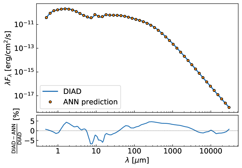
The accuracy of the ANN (i.e., how far the predicted SEDs are from the DIAD ones) was estimated using the blind sample of 5000 additional models, and we adopted a 10 % uncertainty for it (see Appendix B for details). An example of an SED computed with DIAD and the corresponding prediction from the ANN is shown in Fig. 1.

The advantage of the ANN with respect to the standard DIAD models is the time required to evaluate SEDs, which is a few milliseconds. Compared to the $\sim$ 1-2 hours that DIAD requires, this represents an improvement of $\sim 10^{6}$ in computation time, allowing for detailed statistical analysis of large samples of protoplanetary disks.

Figure 1: Top: example of an SED calculated using the DIAD models (solid blue line), and the prediction from the artificial neural network (orange dots) for the same model parameters. Bottom: difference (residual) between the DIAD model and the corresponding prediction. This SED belongs to the blind sample and was not used during the training of the ANN.

2.3 A second ANN for disk masses

The disk mass can be considered as an additional output in the DIAD models, since it is set by the input parameters. The ANN described in Sect. 2.2 cannot determine this quantity because it bypasses all physical calculations and yields the SED directly. However, the models used for the training set in the previous section have disk masses calculated by DIAD, and can thus be used to train a second ANN: one that outputs disk masses as a function of input parameters. We will refer to this second ANN as ANN_diskmass. The value of the disk mass depends on all the DIAD parameters described in Sect. 2.1 except for the inclination of the disk $i$ and the scaling of the wall $z_{\rm wall}$. Thus, it has 10 inputs and one single output, the disk mass. Because ANN_diskmass only predicts one output (which also has a more linear behavior than the SED), a precision of 5 % was achieved using a single layer with 250 nodes (see Appendix B for details).

We note that ANN_diskmass is not used for fitting observations: it simply calculates the disk mass corresponding to a given set of parameters. Once the posterior distributions for the model parameters are derived from the observed SED, they are provided to ANN_diskmass to obtain the posterior distribution of the disk mass as well.

3 Sample

Once the ANN has been trained, it can be used to fit SEDs of protoplanetary disks. In this first study, we focused on the population of protoplanetary disks in the Taurus-Auriga region (see Kenyon et al. 2008, for a review on the region). This association has been a common benchmark for star-formation studies given its proximity (140-160 pc, e.g., Gaia Collaboration et al. 2018) and its young age ($\sim$2 Myr, e.g., Kenyon & Hartmann 1995; Andrews et al. 2013). Numerous studies have identified a population of over 400 young stellar objects (YSOs) in this region, many of them displaying infrared excess characteristic of disk-harboring systems (e.g., Luhman 2004; Monin et al. 2010; Rebull et al. 2010, 2011; Luhman et al. 2017).

In this work, we modeled a sample of 23 objects selected from the 161 T Tauri stars and brown dwarfs with Spitzer/IRS spectra studied in Furlan et al. (2011). We used the dataset presented in Ribas et al. (2017), which merged the photometric compilation for sources in Taurus-Auriga by Andrews et al. (2013) with ancillary photometry, far-IR photometry from the Herschel Space observatory (Pilbratt et al. 2010), and Spitzer/IRS (mid-IR) and Herschel/SPIRE (far-IR/submm) spectra when available. After a number of validation steps in Ribas et al. (2017), the sample was reduced to 154 sources. Additionally, here we included ALMA 1.3 mm photometry from Long et al. (2019).

Recently, Luhman et al. (2017) updated the census of Taurus members, including previous and new spectroscopic measurements of their spectral types (SpTs). We used these SpTs to derive effective temperatures for all the sources in our sample using the relation in Pecaut & Mamajek (2013). We considered sources with $T_{*}$ between 3000 K and 6000 K (corresponding to $\sim$M5 and F9-G0, respectively) to select T Tauri stars, and adopted an uncertainty of 100 K. This temperature range decreases the sample size to 118 objects. We also used a spectral type for Haro 6-13 of K5.5 as reported in Herczeg & Hillenbrand (2014), since the corresponding stellar mass is in better agreement with the dynamical mass estimate in Simon et al. (2019).

Parallax measurements are available from the Gaia DR2 catalog (Gaia Collaboration et al. 2018) for most sources in the sample, and were retrieved by cross-matching the 2MASS coordinates of these objects with the Gaia catalog using a 1 ″radius. Five objects had parallaxes compatible (within uncertainties) with distances smaller than 100 pc or larger than 200 pc, and were discarded.

Several sources were also removed from the sample due to the following reasons:

1. Substructures are ubiquitous in protoplanetary disks (e.g., Andrews et al. 2018a; Long et al. 2018), and their presence requires a more detailed treatment of their radial structure that was not included in our ANN. In particular, inner cavities have an important effect in the SED, and we only considered sources that are not known to have large inner cavities in them. To our knowledge, the list of such sources in our sample includes AA Tau (Loomis et al. 2017), CIDA 1 (Pinilla et al. 2018), CIDA 9 (Long et al. 2018), CoKu Tau/4 (Forrest et al. 2004; D’Alessio et al. 2005), DM Tau (Calvet et al. 2005; Andrews et al. 2011), GG Tau (Guilloteau et al. 1999; Dutrey et al. 2014), GM Aur (Macías et al. 2018), IRAS 04125+2902 (Furlan et al. 2011), IP Tau (Espaillat et al. 2011), LkCa 15 (Piétu et al. 2006; Espaillat et al. 2007, 2008), RY Tau (Isella et al. 2010), UX Tau A (Espaillat et al. 2007), and V410 X-ray 6 (Furlan et al. 2011). In addition, Furlan et al. (2011) also identified other (pre)transitional disk candidates based on their IRS spectra, such as MHO 3, IRAS 04370+2559, GK Tau, JH 112 A, 2MASS J04202606+2804089, and 2MASS J04390525+2337450, and they were also excluded. The presence of rings in the outer regions of the disk does not significantly affect the SED, so we did not remove sources with this morphology (e.g., CI Tau, DS Tau; Clarke et al. 2018; Long et al. 2019).

2. Stellar light from edge-on disks is highly extincted by the disk itself, and their central objects are usually poorly characterized. Models of edge-on disks are also very sensitive to small changes in inclination values, settling, and dust properties, which poses a significant challenge for accurately training the ANN. Therefore, we excluded disks with inclinations $i\geq 70$ °. The edge-on disks in Taurus, as compiled in Furlan et al. (2011), include seven sources: 2MASS J04202144+2813491, 2MASS J04333905+2227207, 2MASS J04381486+2611399, Haro 6-5B, HH 30, IRAS 04260+2642, and ZZ Tau IRS. Additionally, HK Tau B is known to be an edge-on disk (McCabe et al. 2011), Tripathi et al. (2017) found MHO 6 and 2MASS J04334465-2615005 to have inclinations above 70 °, and Long et al. (2019) measured i$\sim$70 °for HN Tau A. These sources were also excluded from our analysis.

3. As mentioned in Sect. 2.1, DIAD computes the emission from the inner wall of the disk based on its temperature and solid angle, which is then re-scaled to account for the unknown true shape of the wall. For almost face-on disks, the solid angle subtended by the wall becomes very small, and a very large scaling factor is required. To avoid training the ANN with a very large range of wall heights, we discarded DR Tau, which has an inclination close to face-on ($i\leq 5$ °, Long et al. 2019).

4. RW Aur, DO Tau, and SU Aur were also removed from the sample because they display long tails of dust and gas. This suggests past flyby encounters, which could have strongly altered the disk structures (e.g., Rodriguez et al. 2018; Winter et al. 2018; Akiyama et al. 2019). Their photometric measurements may also be affected by the surrounding material.

5. Binary stars and multiple systems can have a major impact in the properties, structure, and lifetime of protoplanetary disks (e.g., Artymowicz & Lubow 1994; Cieza et al. 2009; Kraus et al. 2012). Hydrodynamical simulations and detailed information about the system components and orbits are required to take these effects into consideration, and thus we excluded them from our analysis. We cross-matched the list of 133 Taurus sources with companions closer than $<$ 300 au in Kraus et al. (2012) and discarded those that overlapped with our sample. Additionally, we removed the known close binaries DQ Tau (Mathieu et al. 1997), UZ Tau E (Prato et al. 2002), DK Tau and IT Tau (since both components host disks and are closer than 3.5”, e.g., Akeson & Jensen 2014), and the triple system T Tau (Dyck et al. 1982; Koresko 2000).

6. Given the important degeneracies in SED modeling and the number of free parameters involved, we required that the objects have at least one photometric measurement at wavelengths $\geq$ 500 $\mu$m. This requirement ensures that all these objects have coverage up to the submm regime.

We note that some sources meet more than one of these criteria (e.g., binaries can carve gaps in their disks). Thirty-two objects remained after this process. After attempting to fit their SEDs, another 9 objects are discarded (see Sect. 5.1), resulting in a final sample of 23 sources with well-sampled SEDs from the optical to (sub)mm wavelengths and successful fits.

4 Fitting process

4.1 The complete model

Figure 2: Scheme of the complete model used in this study. The input parameters (16 in total) are shown to the left (red). The middle column shows the flow of the model calculation, and each step in the calculation is explained on the right. We note that the stellar mass $M_{*}$ is used both in the MIST isochrones and in the ANN calculations. The final SED obtained through this process, together with tree additional parameters that account for potential outlier photometry, is used to estimate the model likelihood (see Sect. 4.2).

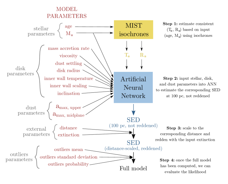
DIAD (and thus the ANN) provides SED estimates based on input parameters, but some additional parameters such as interstellar extinction ($A_{V}$) and distance ($d$) are also needed to model observations. Additionally, although in principle one could use different combinations of the stellar parameters ($M_{*}$, $T_{*}$, and $R_{*}$) in DIAD, most of these combinations are not consistent with stellar evolution. Thus, every model computed in our fitting procedure explored different values of stellar and disk parameters, $A_{V}$, and distance following these steps:

1. The two fundamental parameters that determine stellar properties in our modeling procedure are the age and mass of the star ($M_{*}$). Therefore, we adopted these two as input free parameters in our model. For any given age-$M_{*}$ pair, the first step was to use the MESA Isochrones and Stellar Tracks (MIST, Paxton et al. 2011, 2013, 2015; Dotter 2016; Choi et al. 2016) to obtain the corresponding $T_{*}$ and $R_{*}$ values. We note that $T_{*}$ and $R_{*}$ are determined by the age and $M_{*}$ and thus are not free parameters in the model. Although age is not a free parameter in DIAD, we used this approach to ensure that the combinations of $M_{*}$, $T_{*}$, and $R_{*}$ explored during the fitting process are consistent with evolutionary tracks and that its effect in the uncertainties of other parameters is accounted for in our results.

2. This set of consistent stellar parameters is fed to the ANN together with the remaining disk and dust parameters: the mass accretion rate ($\dot{M}$), the disk viscosity ($\alpha$), dust settling ($\epsilon$), the maximum grain sizes in the disk atmosphere and midplane ($a_{\rm max,upper}$ and $a_{\rm max,midplane}$), the disk size ($R_{\rm disk}$), the inclination ($i$), the dust sublimation temperature ($T_{\rm wall}$) and the scaling factor of the inner wall ($z_{\rm wall}$). The ANN then yields the corresponding SED at 100 pc, and without any interstellar extinction.

3. The SED output from the ANN is then scaled to the corresponding distance ($d$), and reddened by $A_{V}$ using the extinction law by McClure (2009) following Ribas et al. (2017). $A_{V}$ is the interstellar extinction, and does not include the self-extinction produced by the disk itself (which is already accounted for in DIAD when needed).

With this setup, the model has 13 free parameters: the age and mass of the central source (which determine the remaining stellar parameters through the MIST isochrones), the remaining DIAD parameters, and the distance and interstellar extinction to the source. Additionally, three more free parameters were included to account for possible outlier fluxes (see Sect. 4.2.3). Therefore, there are a total of 16 free parameters involved in the modeling process, all of which are varied during the fitting to compute posterior probability distributions. A scheme of the complete model is shown in Fig. 2.

4.2 The Bayesian framework

Our model has a significant number of free parameters, some of which are unconstrained by observations, degenerate, or may have multimodal posteriors. For these reasons, we adopted a Bayesian framework in our analysis, which allows us to incorporate pre-existing information about some of the model parameters, as well as to naturally account for unconstrained/uncertain parameters in the resulting posterior distributions.

4.2.1 Photometric and spectroscopic uncertainties

Uncertainties of the observed data are crucial in model fitting, since underestimated uncertainties can give excessive weight to some data points and bias inference results. In our case, the photometric data were mostly gathered from the comprehensive compilation by Andrews et al. (2013), which used tens of studies to create SEDs for YSOs in the Taurus-Auriga region. While this yielded detailed SEDs for most objects, the heterogeneous origins of the data imply that their uncertainties were also estimated in different ways and, in some cases, could be missing systematic uncertainties. Therefore, we set the minimum relative uncertainty to 10 % for all the photometry to account for the heterogeneity of the data.

We also face a problem when fitting both photometry and spectra together: Because spectra have a much larger number of data points, the fitting process is dominated by these, even though they may only cover a fraction of the whole wavelength range probed by the SEDs. While there is no standard procedure to take this into account, we tried to mitigate this effect by weighting the spectra so that they correspond to a certain (smaller) effective number of points $N$. This is achieved by increasing their uncertainties by a factor of $\sqrt{N_{\rm spectrum}/N}$, where $N_{\rm spectrum}$ is the number of points in the corresponding spectrum. After various tests, we found $N$=10 and $N$=5 to be good compromises for the weights of IRS and SPIRE spectra, respectively (although the SPIRE spectra are featureless, the IRS ones contain the silicate features at 10 and 20 $\mu$m, informative of the properties of small grains in the disk atmosphere). We note that these numbers do not have a physical justification and were chosen heuristically.

4.2.2 Priors

Bayesian analysis requires the use of priors, which encompass pre-existing knowledge of the parameters (both from physical arguments or previous measurements). For most parameters, we chose either flat or Jeffreys priors (which we used for parameters that could change by orders of magnitude to give equal probabilities to each decade interval) within reasonable ranges. Our tests also showed that using uniform priors instead of Jeffreys did not significantly alter the results. For the inclination, we used a Gaussian distribution when an observational measurement exists, otherwise the observational prior was used (i.e., uniform in $\cos(i)$; see Appendix C.2). For the distance, an observational prior (i.e., proportional to $d^{2}$) between 100 and 200 pc was used (an additional term is included in the likelihood for sources with available parallax information from the Gaia DR2, see next section and Appendix. D). We did not include prior information about disk sizes from resolved observations given their strong dependence on the wavelength due to dust radial migration (e.g., Tazzari et al. 2016), which is not included in our models. A complete list of the priors used as well as the references for inclination measurements (when available) are provided in Appendix C.

Figure 3: SEDs of the 23 sources successfully fit in this study. The observed photometric data (orange dots) and the IRS/Spitzer and SPIRE/Herschel spectra (orange line, when available) are shown. We also plot the results of the modeling process by randomly selecting 1000 models (blue lines) from the posterior distributions.

4.2.3 Likelihood functions

For each object, up to four different datasets can exist in our sample, namely: photometry, spectroscopy (from IRS/Spitzer, SPIRE/Herschel, or both), a SpT measurement, and a parallax value from the Gaia DR2. Therefore, our likelihood function contains up to four different terms, and can be expressed as:

$$\mathcal{L}=\mathcal{L}_{\rm phot}\,\mathcal{L}_{\rm spect}\,\mathcal{L}_{\rm T_{*}}\mathcal{L}_{\rm parallax}.$$ (1)

These likelihood functions follow the standard case for Gaussian uncertainties. Additionally, the photometric likelihood incorporates a mixture model to account for potential outlier photometric points. The mathematical description for each of these is provided in Appendix D. For objects with no parallax measurement available, the parallax term $\mathcal{L}_{\rm parallax}$ is not included in the likelihood.

Only photometric data between 0.5 $\mu$m and 5 mm were used for the fitting process: shorter wavelengths may include significant emission from accretion shocks, which is also highly variable (e.g., Ingleby et al. 2013; Robinson & Espaillat 2019), while longer ones could be affected by free-free emission from photoevaporative winds or gyrosyncroton emission from stellar activity (Pascucci et al. 2012; MacGregor et al. 2015; Macías et al. 2016).

4.3 Estimation of posterior distributions

Once the prior and likelihood functions were defined, we evaluated the posterior distribution of each object using the emcee (Foreman-Mackey et al. 2013) Python implementation of the Goodman & Weare’s Affine Invariant Markov Chain Monte Carlo ensemble sampler (Goodman & Weare 2010). We used 50 walkers in each case, and their initial positions were randomly distributed within the prior ranges. To avoid individual walkers getting stuck in local minima, we first ran 25000 steps. We then used the median and standard deviation of the walker positions to define a second set of locations from where we ran 75000 more steps, adding up to a total of 100000 steps. The autocorrelation times of the chains were then computed, and we checked that they were smaller than a tenth of the chains length. If that was not the case, the chain was evolved for another 10000 steps, and the process was repeated until the criterion was met. Finally, another 5000 steps were run to estimate the posterior distributions. The masses corresponding to these final 5000 steps were also computed using ANN_diskmass as described in Sect. 2.3 to create the probability distributions for this quantity.

Figure 3: (Continued).

5 Results

5.1 Successful fits and discarded sources

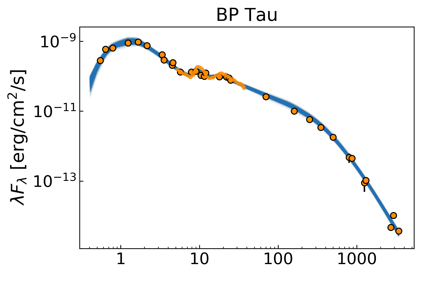
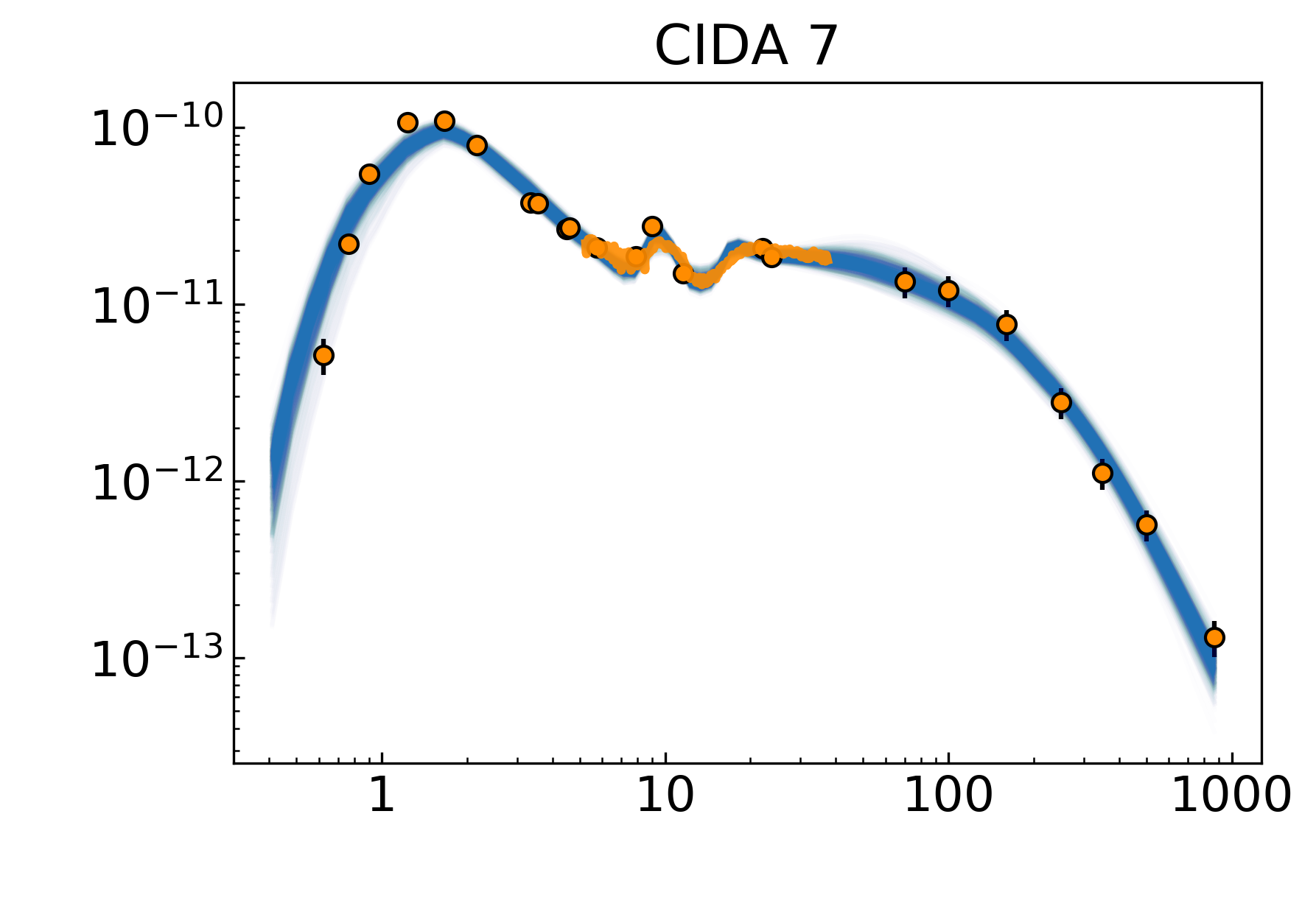
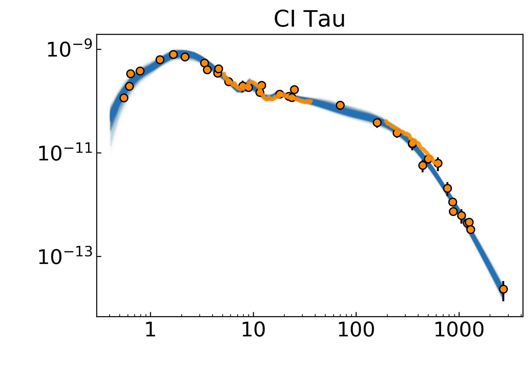
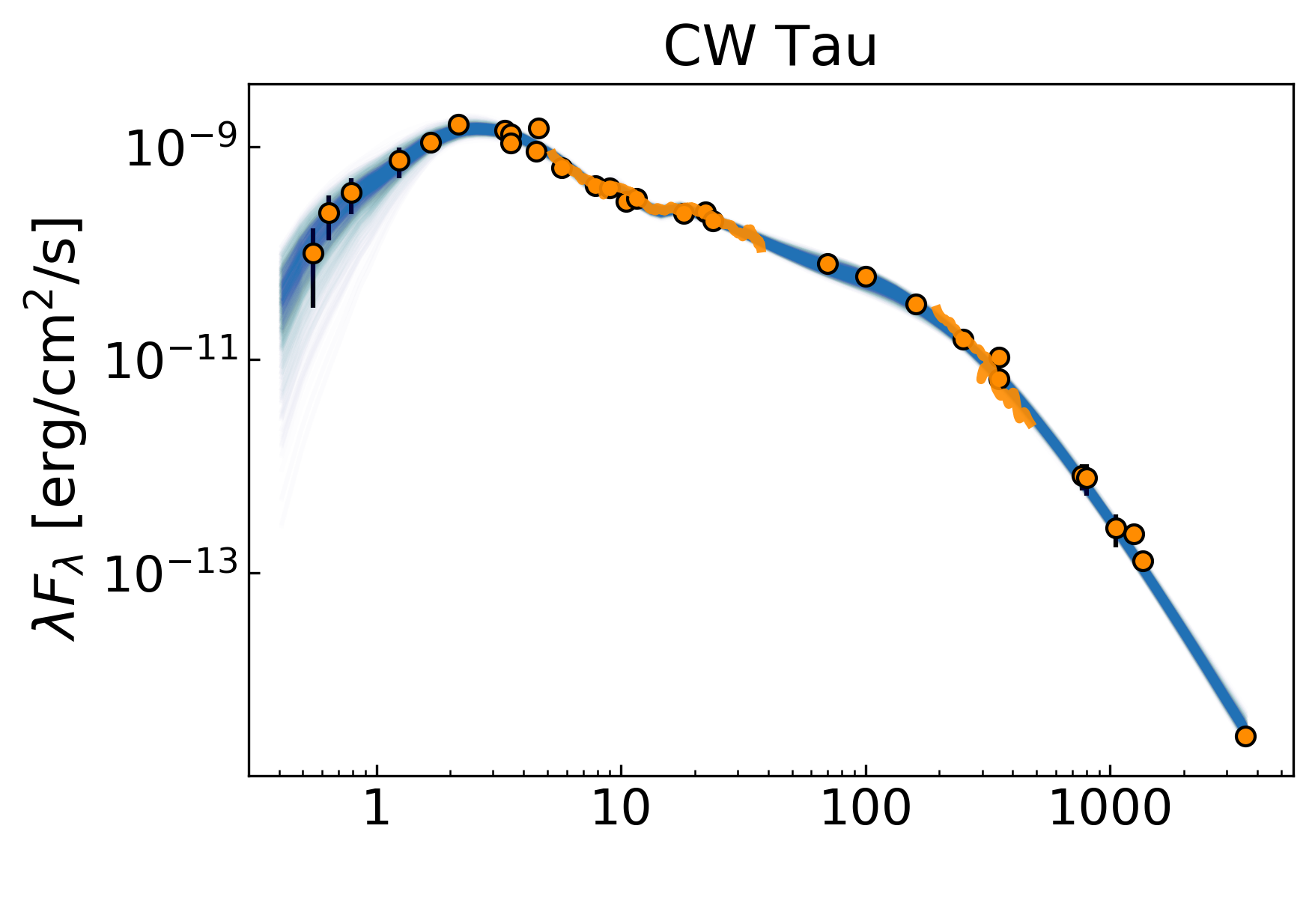
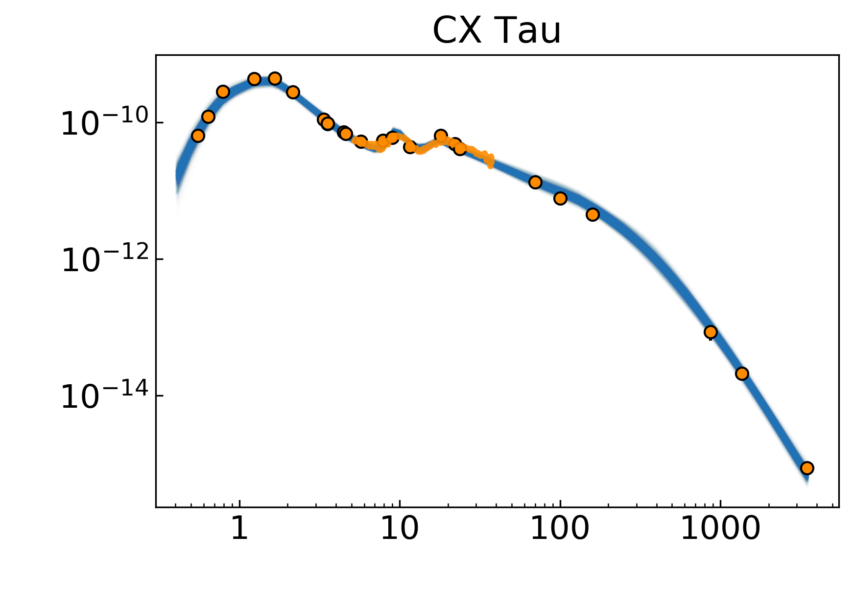
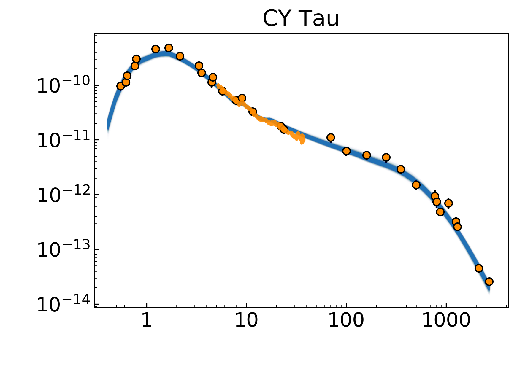
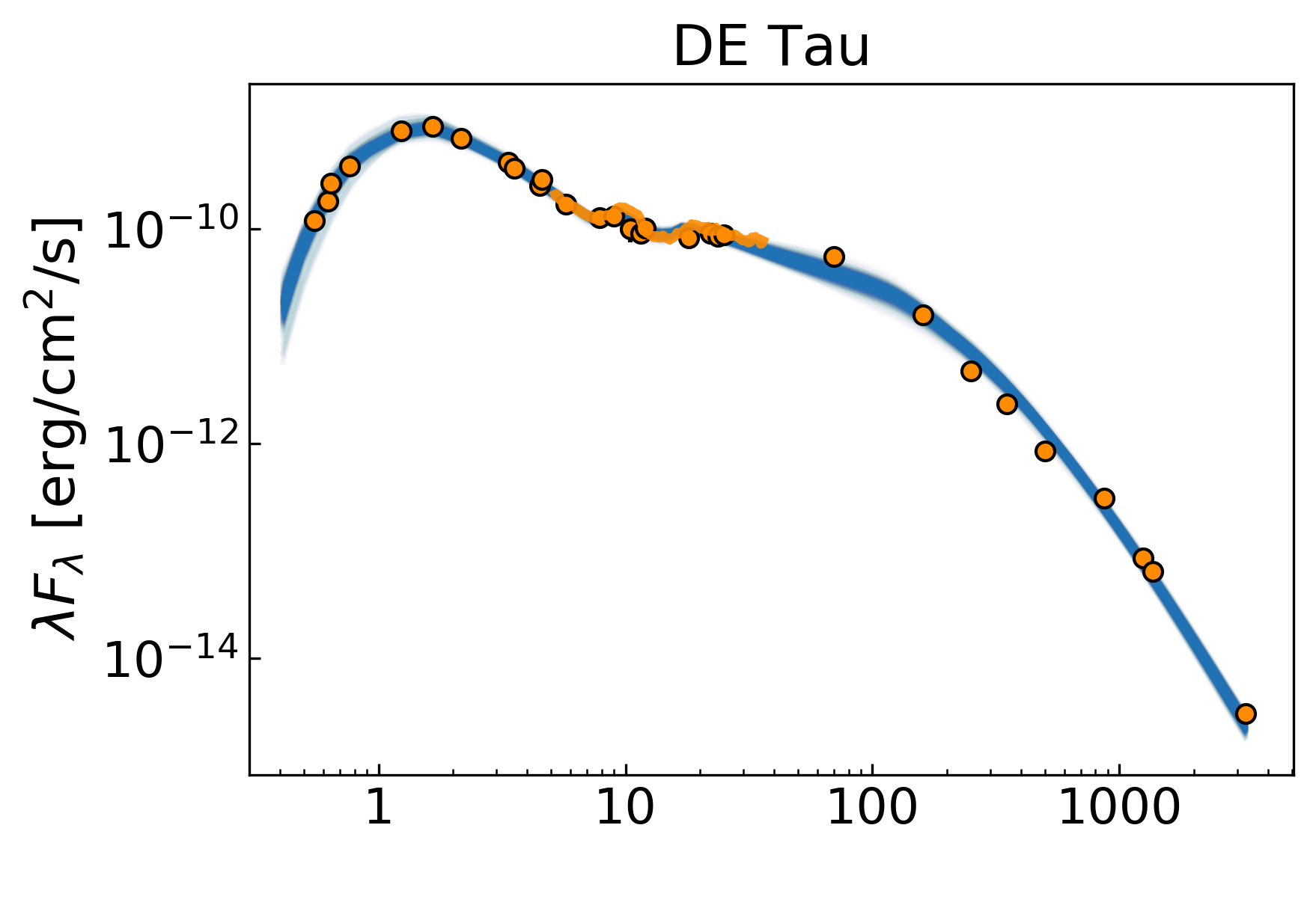
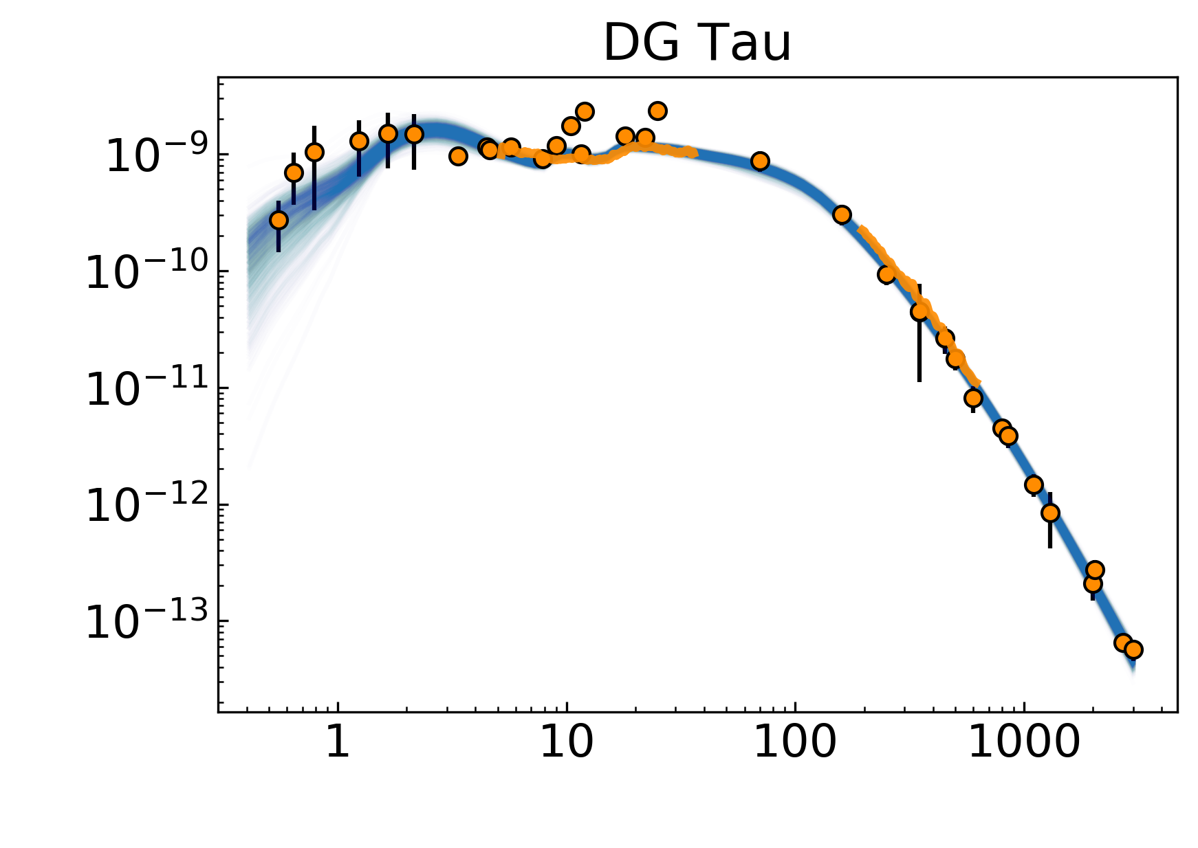
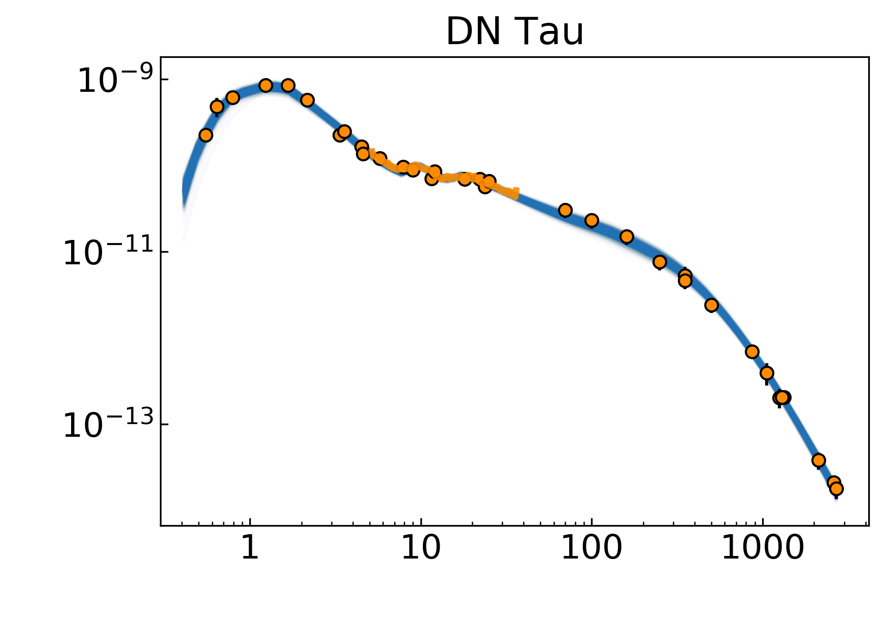
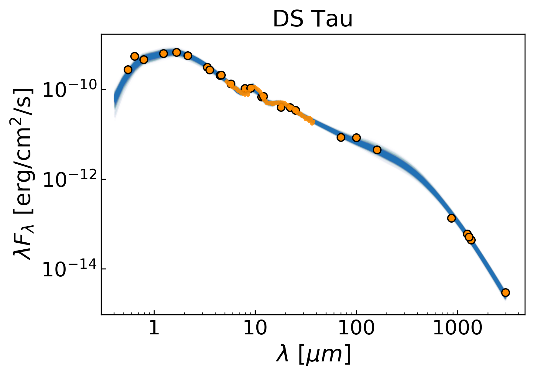
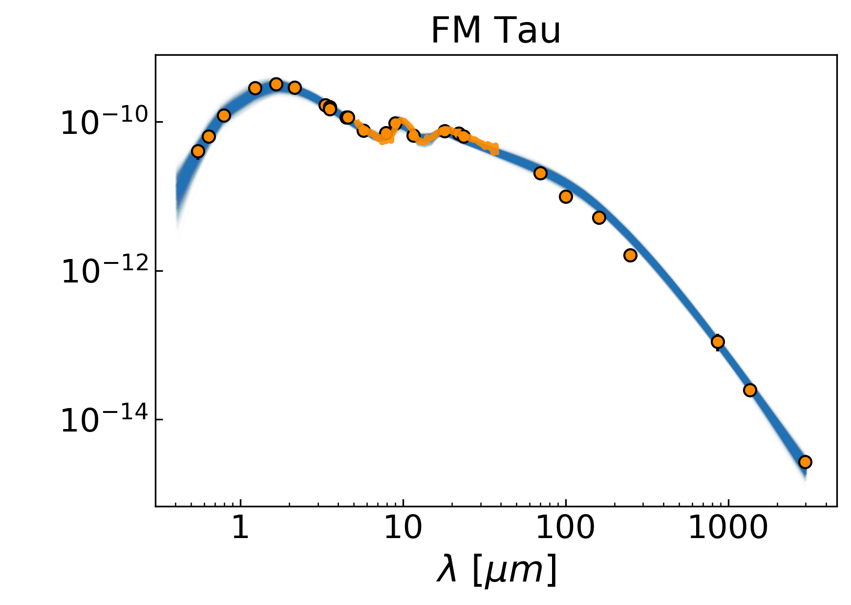
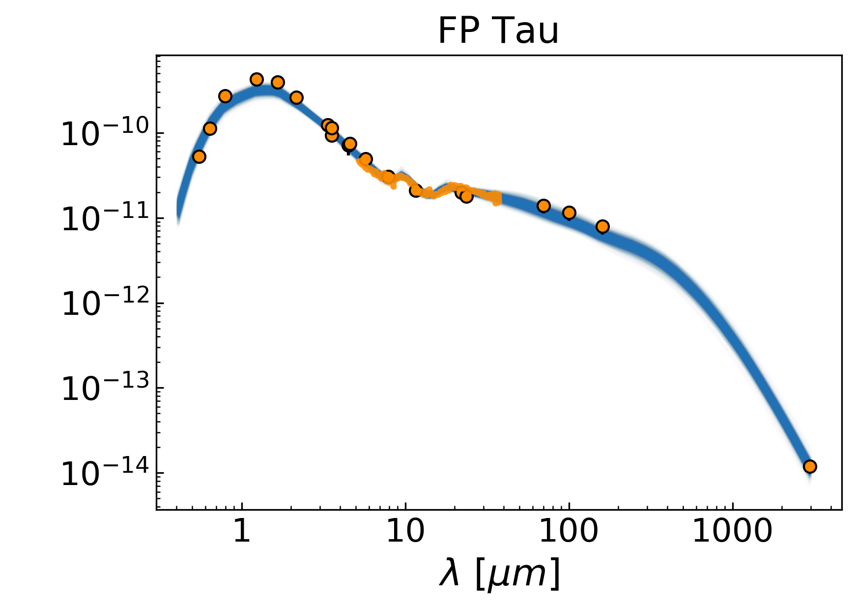
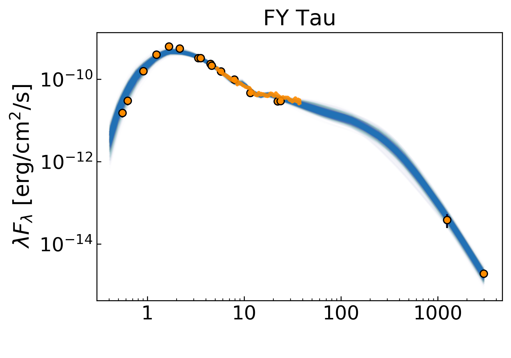
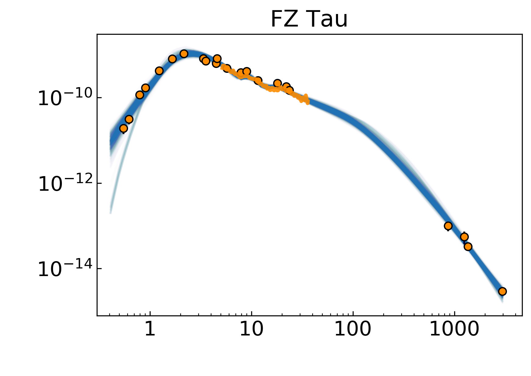
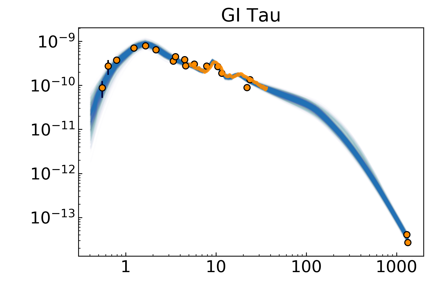
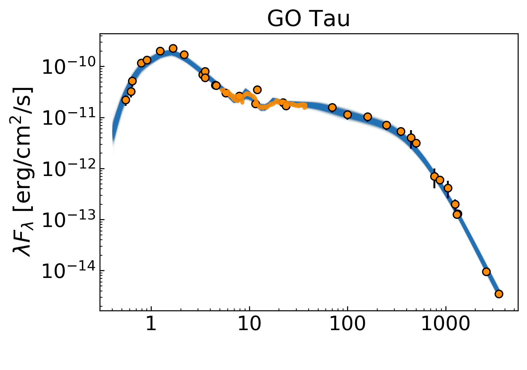
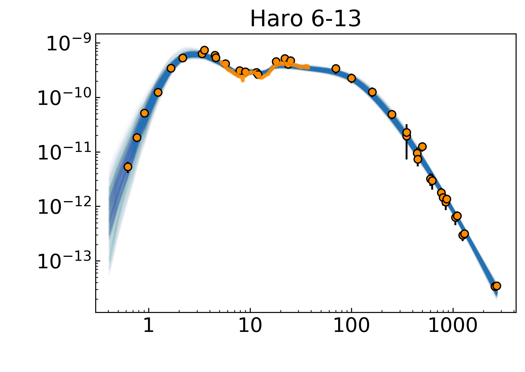
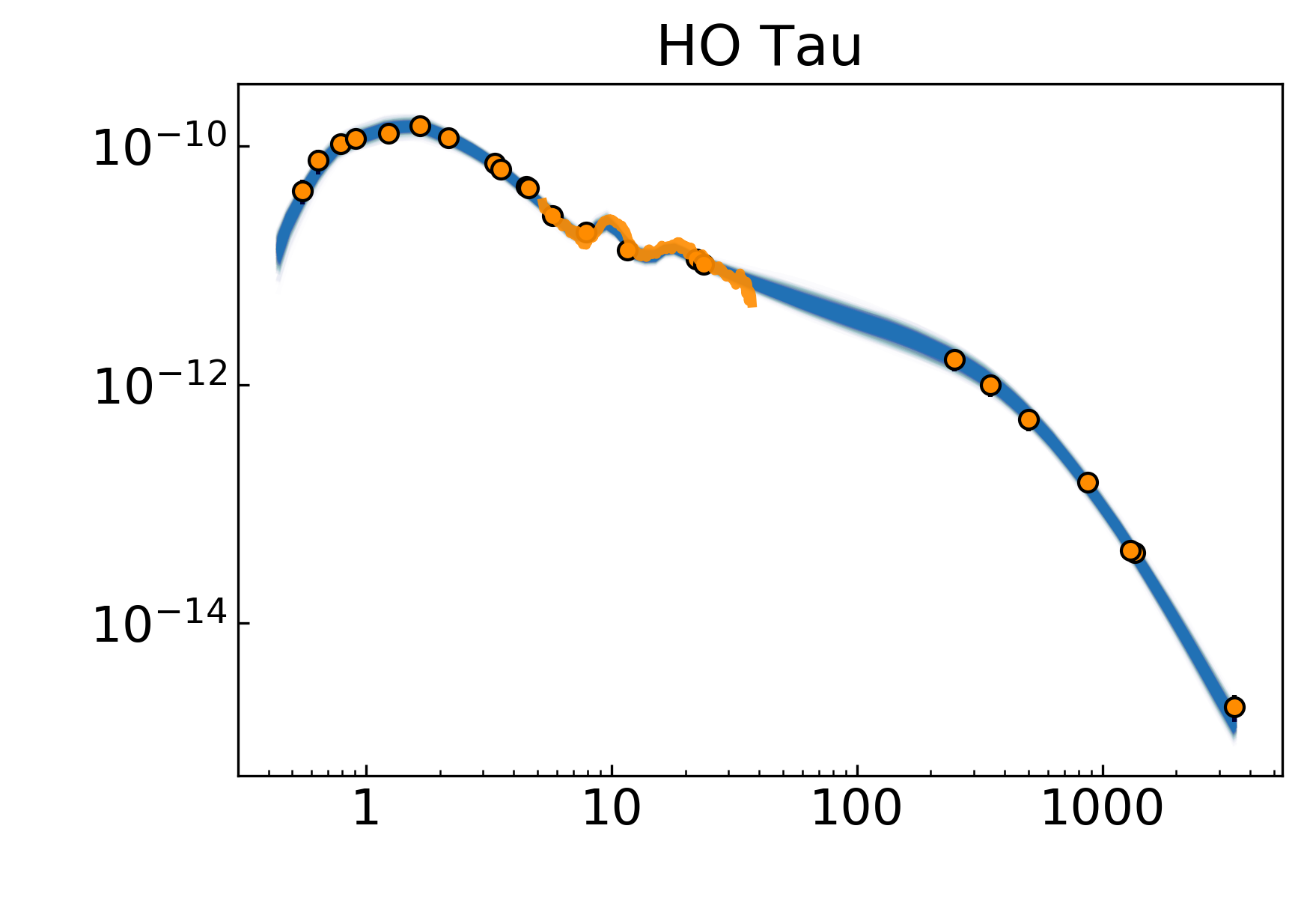
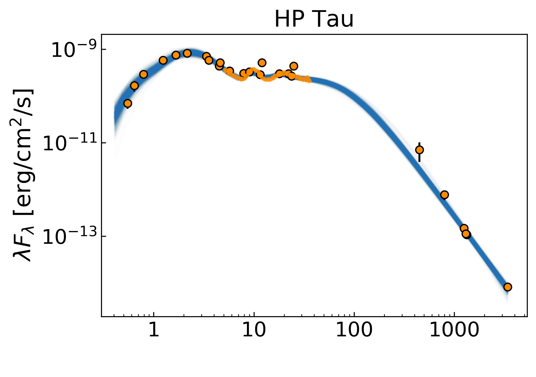
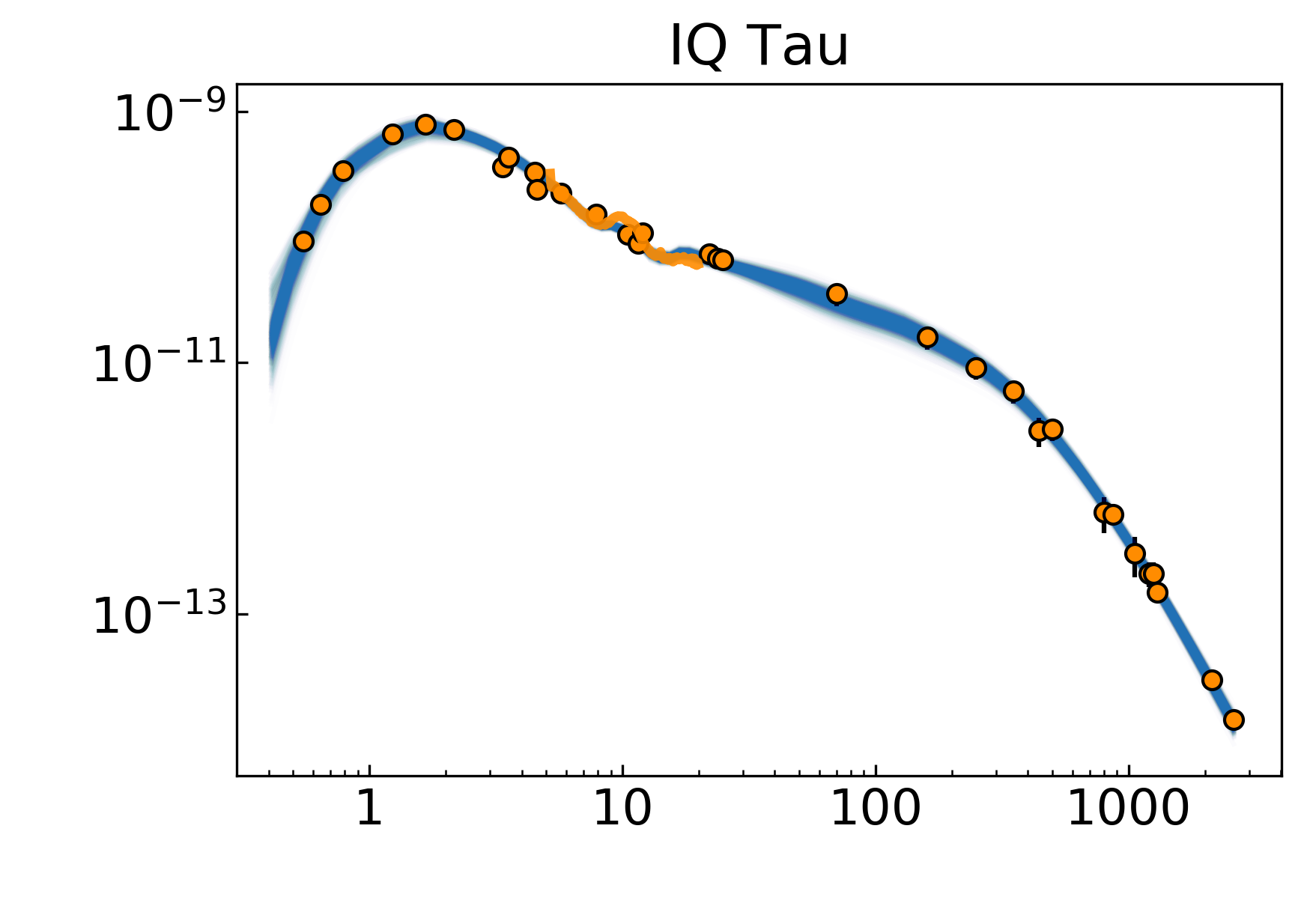
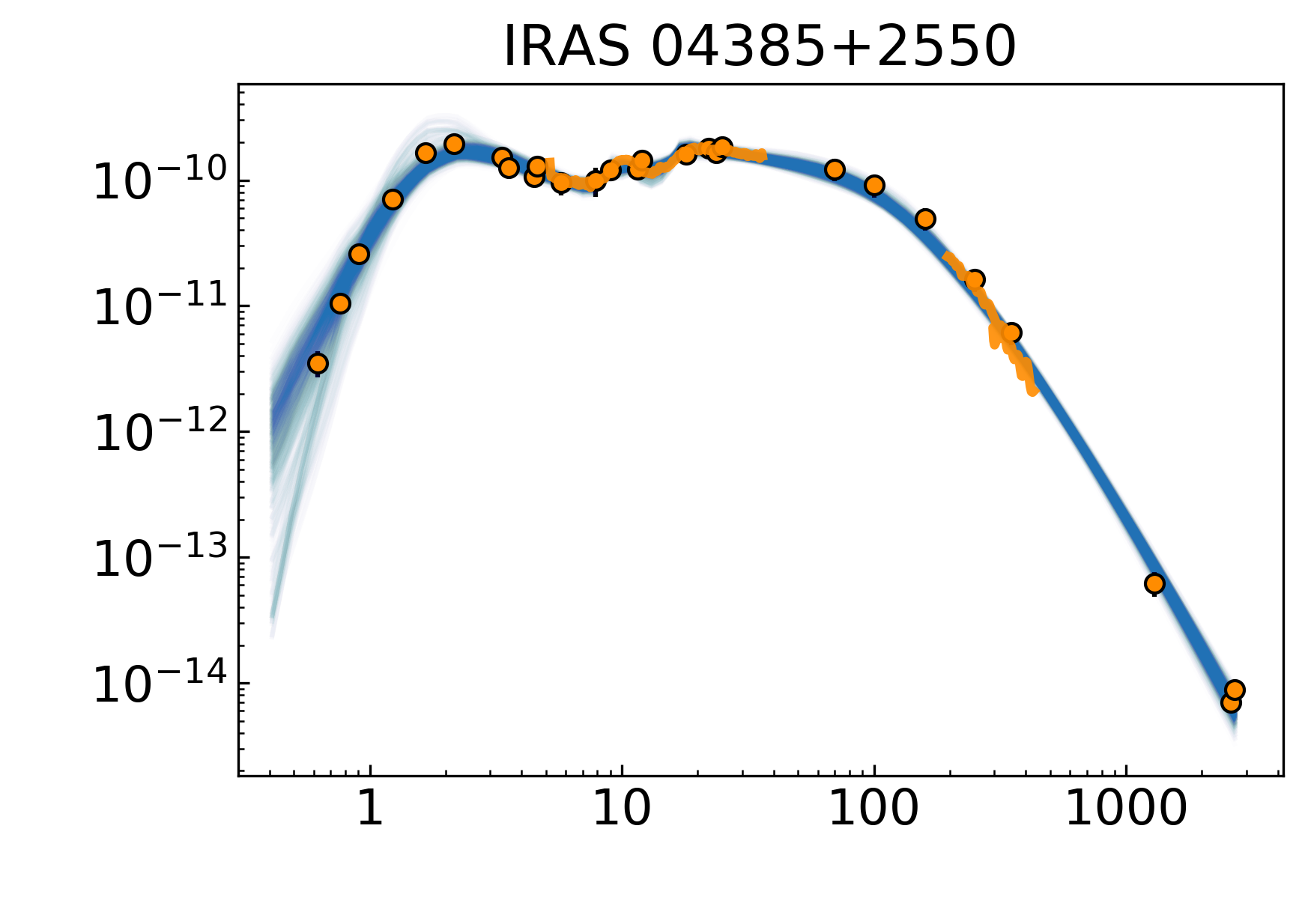
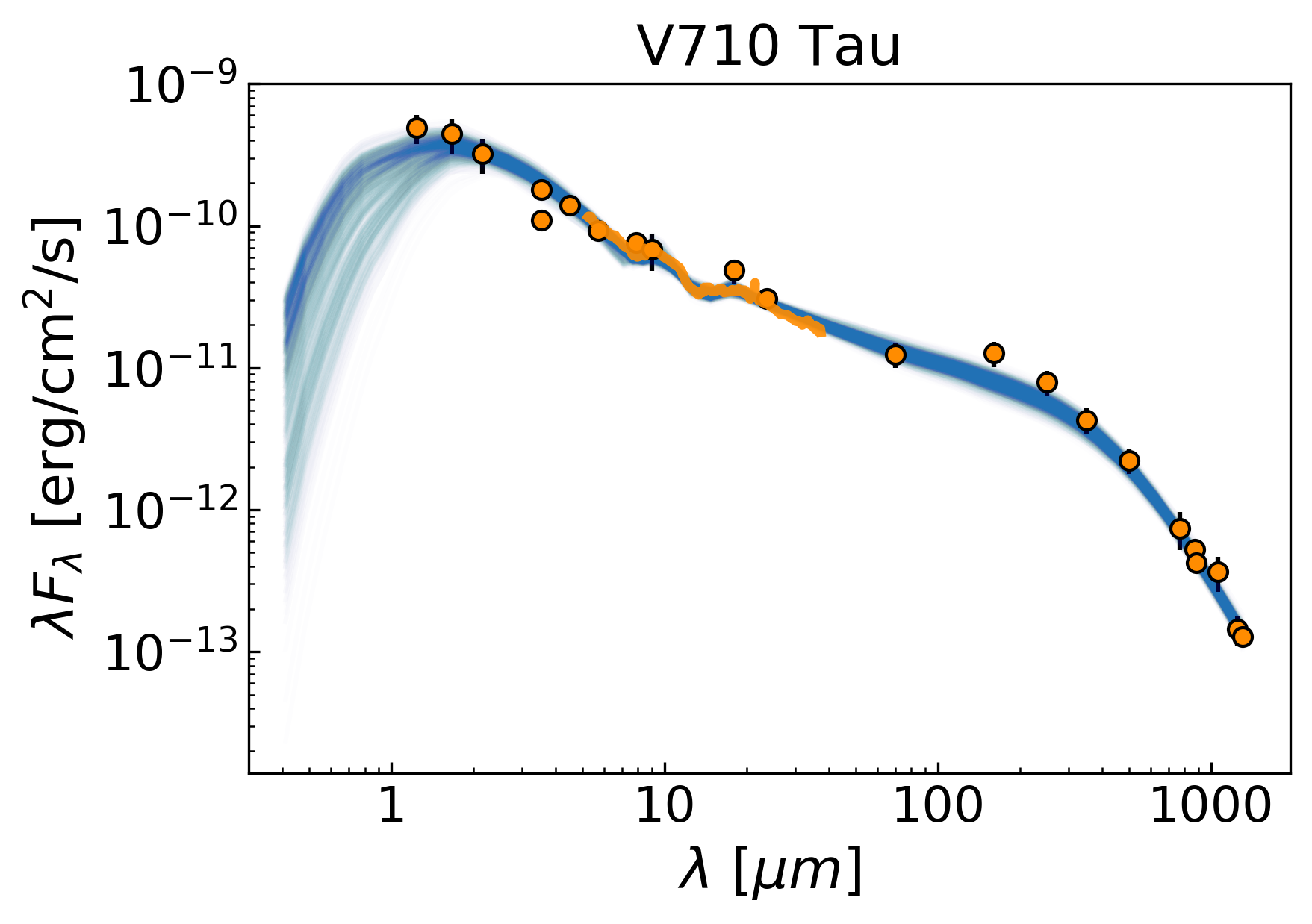
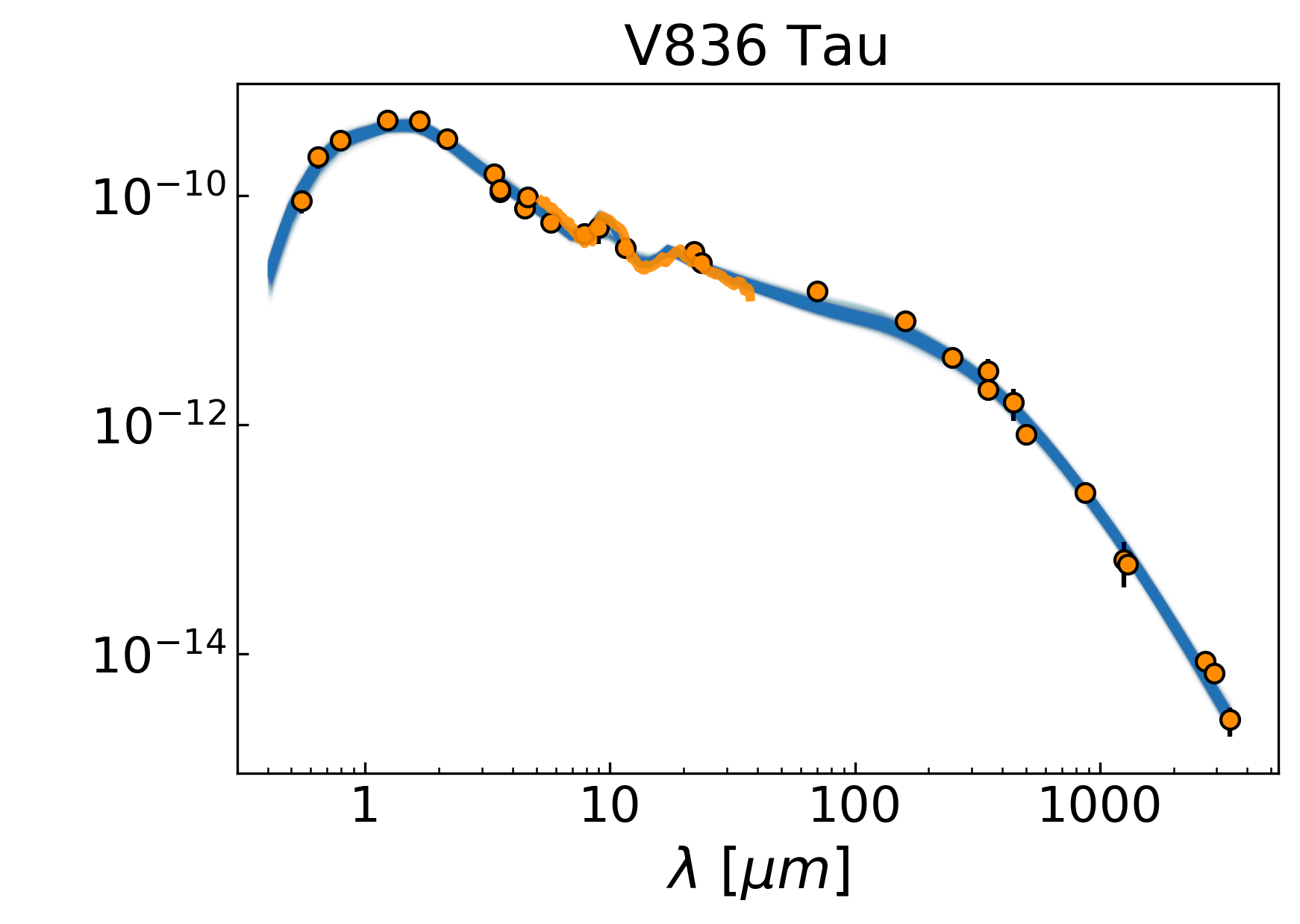
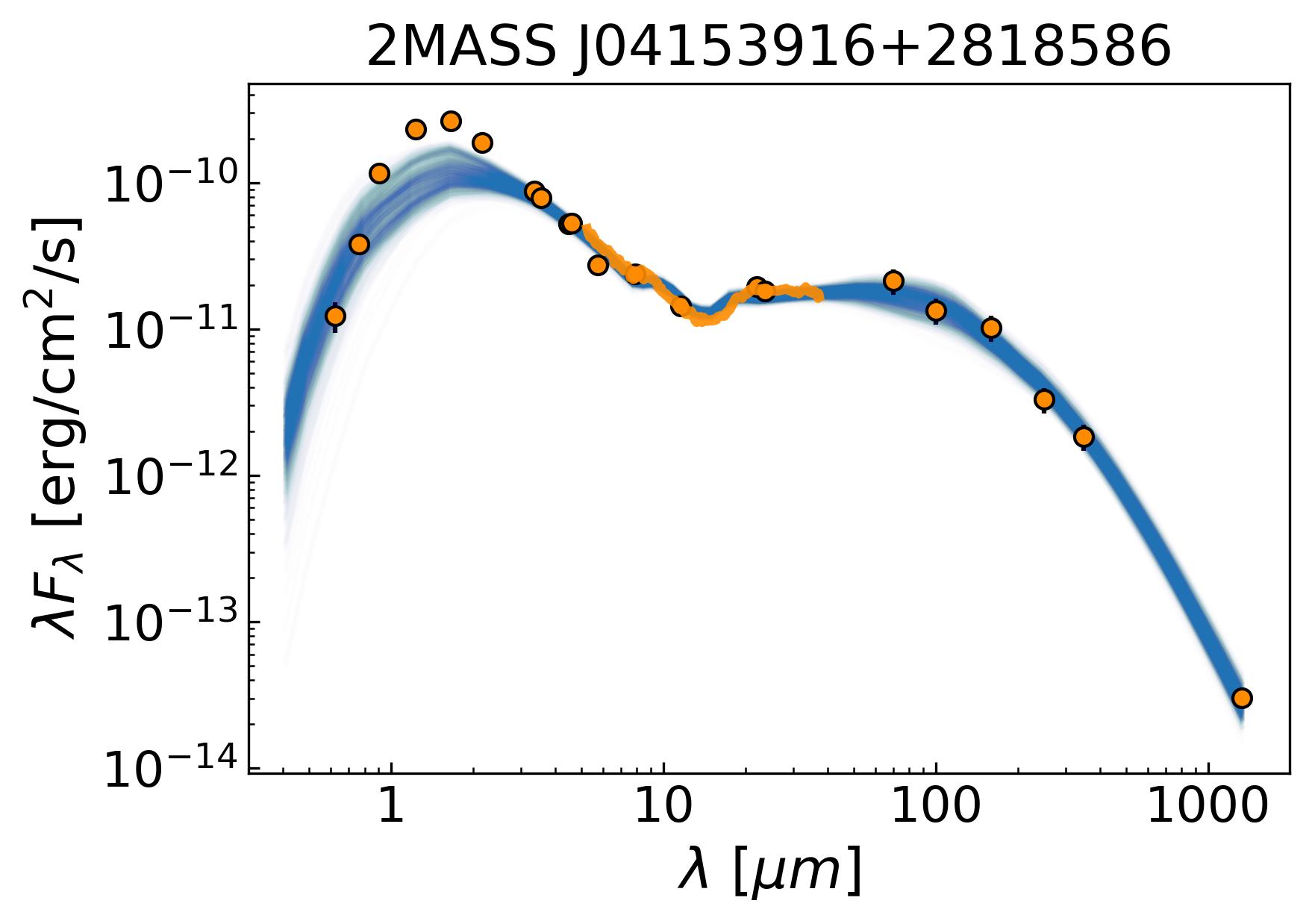
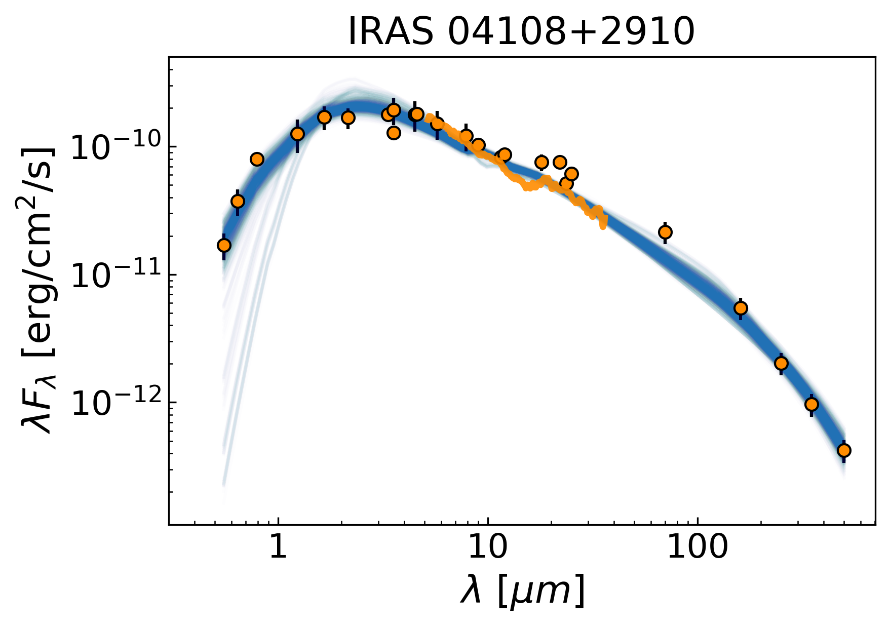
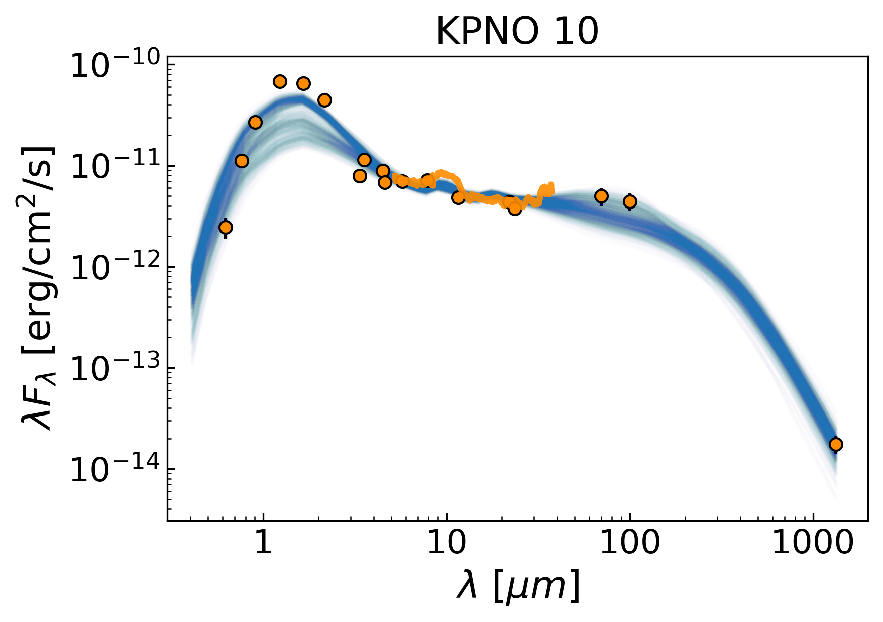
It is likely that some disks in the sample have yet unknown substructures or companions, or are affected by physical processes not considered in our modeling. Thus, some objects may not be properly described by the DIAD models, and it is expected that we will not be able to fit the whole sample successfully. Before analyzing our results, we inspected the obtained fits and discarded those sources for which the models were unable to reproduce the observed SED. Nine objects were discarded during this process: 2MASS J04153916+2818586, DL Tau, FN Tau, IRAS 04108+2910, IRAS 04196+2638, IRAS 04216+2603, IRAS 04200+2759, KPNO 10, and XEST 13-010. Therefore, the final sample of successfully modeled disks comprises 23 sources. Their SEDs and corresponding models are shown in Fig. 3. For reference, we also show three discarded cases in Fig. 4.

5.2 Results for parameters of interest

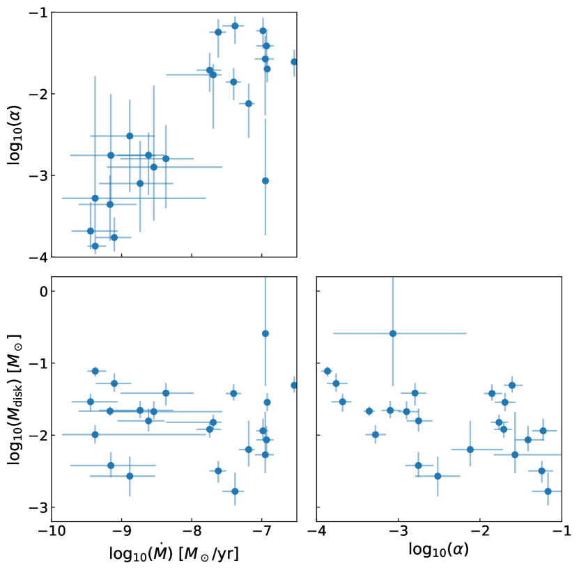
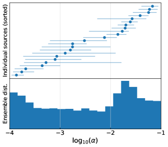
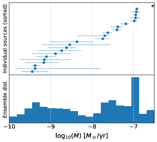
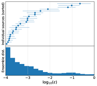
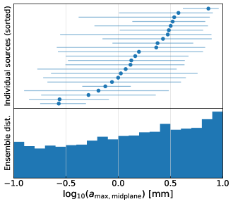
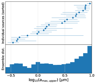
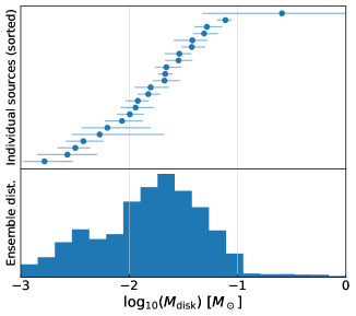
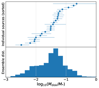
Our goal is to better understand the general properties of disks without focusing on individual objects, since better fits could probably be achieved by considering the characteristics of each source in detail. For this purpose, we built the ensemble distribution for each parameter by randomly drawing 1000 values from the posterior of each source, and combining them in a joint histogram (see Fig. 5). Nevertheless, the results of the parameters of interest for individual sources are listed in Table 2, and the corresponding cornerplots can be retrieved from an online repository. Some parameters in our model are nuisance ones and, in those cases, we marginalized over them (see Appendix F).

5.2.1 Disk viscosity and accretion rate

As mentioned in Sect. 2.1, the ratio of these two parameters determines the scaling of the surface density profile ($\Sigma\propto\dot{M}/\alpha$, e.g., D’Alessio et al. 1998). Therefore, these two parameters are correlated. However, their effects on the SED at mid/far-IR wavelengths allow us to constrain them individually as well: when maintaining a constant ratio between these two parameters, higher accretion rates increase the accretion luminosity irradiating the disk, which heats the upper layers and increases the mid/far-IR disk emission (see bottom right panel of Fig. 7). Both parameters are relatively well constrained for most sources. In the case of $\alpha$, the obtained median value is 0.003 and a significant fraction of the sample (10 out of 23 objects) is above $\alpha=0.01$, with individual values distributed throughout the entire explored range ($1\times 10^{-4}$ to 0.1). These results are compared with observations in Sect. 6.1. For the accretion rates, the median ($2\times 10^{-8}\,M_{\odot}$/yr) is in good agreement with previous results (Hartmann et al. 1998). Despite the accretion rate in the disk and that onto the star not being the same parameter and the significant variability of the latter, we find an overall agreement (within an order of magnitude) of our derived accretion rates and those reported in the literature (e.g., Valenti et al. 1993; Hartigan et al. 1995; Gullbring et al. 1998; Ingleby et al. 2013; Simon et al. 2016).

5.2.2 Disk radius

Disk sizes are poorly constrained by SED fitting alone, and we do not expect the derived radii to be very accurate. Moreover, dust radial migration causes grains with different sizes to have different radial extents and, therefore, the observed radii depend on the wavelength (e.g., Tazzari et al. 2016). Our models do not account for this effect and, since we fit emission at all wavelengths, our radii estimates should be either larger or comparable to radii at millimeter wavelengths (for sources with or without significant dust radial migration, respectively). The ensemble distribution shows a rather unconstrained distribution (with a little preference for larger radii), except for a family of sources with radii $\leq$50 au. Interestingly, this trend seems to reflect a population of compact disks recently discovered with high-spatial resolution ALMA observations (e.g., Cieza et al. 2019; Long et al. 2019).

5.2.3 Dust settling

As discussed in Sect. 2.1, the DIAD models include two layers with different dust grain populations to simulate dust settling (small grains in the upper layers, larger grains in the disk midplane). The $\epsilon$ parameter describes the depletion of grains in the upper layers with respect to the standard gas-to-dust ratio. Our results show high levels of settling ($\epsilon<10^{-2}$) for the whole sample, indicating that disks in Taurus-Auriga have already undergone significant settling, in agreement with previous studies (Furlan et al. 2011; Grant et al. 2018). Given that this process concentrates large grains in the disk midplane and enables planet formation, this is in line with the ubiquity of rings and gaps found in protoplanetary disks if these structures are to be explained by the presence of planets.

5.2.4 Grain sizes

The size of grains in the upper layers of disks ($a_{\rm max,upper}$) is mostly determined from mid-IR spectroscopy and, in particular, from the shape of the silicate features at 10 and 20 $\mu$m. Given that our sample includes Spitzer/IRS spectra for all objects, we expect to gain some information about $a_{\rm max,upper}$. Indeed, the results for this parameter suggest that grains of a few $\mu$m are present in the upper layers of these disks, but the derived values are general estimates only (see Sect. 5.3). On the other hand, information about large grains in the midplane ($a_{\rm max,midplane}$) is usually assumed to come from (sub)mm fluxes, and the slope of the mm emission has been used for this purpose under some assumptions (e.g., Ricci et al. 2010a, b; Ribas et al. 2017). However, although many of our sources have well-sampled SEDs in this wavelength range, the ensemble distribution of $a_{\rm max,midplane}$ is poorly constrained, with only a slight trend toward large ($>1$ mm) grains. The lack of strong evidence for large grains in our analysis is somewhat surprising, and could imply that the combined effect of other parameters in grain size uncertainties may have been previously underestimated when establishing grain growth in disks (e.g., Ysard et al. 2019). Our results suggest that very little information about grain sizes in the disk midplane can be gained from SEDs alone.

Figure 4: Three examples of SEDs that we were not able to properly fit with our adopted model. Symbols are the same as in Fig. 3.

5.2.5 Disk masses

The disk mass ($M_{\rm disk}$) is one of the most relevant quantities in planet formation. Despite $M_{\rm disk}$ not being a free parameter in the DIAD models, we can estimate the disk mass of each model in the posterior distributions using ANN_diskmass. This yielded the corresponding $M_{\rm disk}$ distribution for each source, which is well constrained in all cases. We then computed the ensemble posterior for the 23 sources as in Sect. 5.2. The derived disk masses are listed in Table 2, and the results for $M_{\rm disk}$ and $M_{\rm disk}/M_{*}$ are shown in Fig. 5. The ensemble distribution of $M_{\rm disk}$ peaks at $0.02\,M_{\odot}$, and is smoothly distributed between 0.001 and 0.1 $M_{\odot}$. In the case of $M_{\rm disk}/M_{*}$, we found it to range from 0.003 to 0.3, with a preference for values between 2-10 %. The distribution decreases rapidly for higher values, in agreement with general disk stability criteria (e.g., Lodato & Rice 2005). Given that $M_{\rm disk}$ is proportional to the ratio $\dot{M}/\alpha$ in the $\alpha$-disk prescription, we also searched for possible correlations of $M_{\rm disk}$ with those parameters. Despite $\dot{M}$ and $\alpha$ showing a clear correlation (as expected for $\alpha$-disk models), none of them appear to be significantly correlated with $M_{\rm disk}$ in our results (see Fig. 13).

One advantage of the method employed in this study is that it does not require some of the standard assumptions when estimating disk masses from (sub)mm observations (e.g., emission from isothermal dust, optically thin emission) and, given the Bayesian framework used, it naturally accounts for the effect and uncertainties from all the other parameters. However, the caveats in Sect. 5.3 should be considered when using these disk mass estimates. In particular, we note that the gas-to-dust value is highly uncertain and, therefore, the dust content should be more accurate than the total (gas+dust) mass.

5.3 Caveats

Although we have tried to account for as many uncertainties and physical phenomena as possible during our analysis, it is important to consider the caveats in our models and the implications they may have in our results.

We have not explored different dust compositions, which has a crucial effect on the dust opacity and, therefore, on the thermal structure of disks. Including this factor in our models adds a considerable number of free parameters, which would significantly increase the complexity of the ANN training. Moreover, a proper exploration of dust compositions requires a detailed fitting of the Spitzer/IRS mid-IR spectra and, as explained in Sect. 4.2.1, we have weighted the spectroscopic data heuristically in our study. While this makes the overall fitting more consistent, it also decreases the quality of the fit to the spectra. Thus, we chose to keep the dust composition fixed. As a result, the derived sizes for grains in the upper layers are approximations.

We have adopted the standard gas-to-dust ratio value of 100 in our models. This parameter affects the gas density in the disk and, therefore, its structure. Given the various difficulties in determining this quantity, this choice allows us to compare our results with other studies and to test default assumptions about disk properties. However, it is very likely that the gas-to-dust ratio changes considerably from source to source (e.g., Bergin et al. 2013; Williams & Best 2014; Schwarz et al. 2018).

Our models also assume disks with no substructures, (i.e., no rings in their surface density profiles). We have excluded sources with known large cavities from our sample, but this does not guarantee that the modeled disks have smooth density distributions since not all the remaining objects have been observed at high-spatial resolution and, even then, the presence of smaller, unresolved substructures cannot be ruled out. In fact, a few sources in our sample are known to harbor rings in their outer regions. Nevertheless, we note that most disk substructures are likely produced by trapping of large particles in pressure bumps (e.g., Dullemond et al. 2018), so the distribution of smaller ($<$1 mm) particles, which dominate the SED emission, is probably less affected by possible substructures.

We have not performed any convolution of the models with the corresponding photometric filters when computing the likelihoods. This could be relevant mostly at optical and near-IR wavelengths due to stellar absorption lines (at longer wavelengths, the flux is dominated by the mostly line-free continuum emission from the disk). However, since we enforce that the resulting stellar temperatures match the observed ones and use isochrones to guarantee consistent stellar parameters, this should have little to no impact on the modeling results, especially for disk parameters.

We do not account for stellar scattered light, which is usually a negligible contribution with respect to the stellar and disk thermal emission in cases where the disks are not highly inclined (e.g., D’Alessio et al. 2006). Since we have removed disks with high inclinations, the impact of scattered light in our results should be minor. We note that a high polarization fraction has been found in a couple of sources in our sample (DG Tau and Haro 6-13 show polarization fractions of $\sim$4.4 % at J band, Moneti et al. 1984), which indicates that they could have a more relevant contribution from stellar scattered light. However, as in the previous case, the observed stellar temperatures and parallaxes from the Gaia DR2 provide strong constraints for the stellar parameters and they should not be significantly affected by this issue.

Finally, our sample represents only a subset of disks taken from a single star-forming region. Therefore, these results are likely representative of disks with no large gaps around single T Tauri stars only, and may not be applicable to all disks; those with significant substructures or in multiple systems could have different physical conditions. Moreover, the details of the ensemble distributions in Fig. 5 are probably caused by the moderate sample size, and only the overall trends in them are likely real. Extending this analysis to other regions will allow us to increase the sample size and to determine which structures in the ensemble distributions are in fact real.

Figure 5: Results for individual sources (top panels) and ensemble distribution (bottom panels) of each relevant parameter for the sample of 23 disks modeled in our study. The top panels show the parameter value (blue dot) for each source, sorted by increasing value. The errorbars are the corresponding 16 % and 84 % percentiles. The ensembles in the bottom panels show the overall distribution of the sample, and are produced by randomly selecting 1000 values from the posterior distribution of each object, and then combining all of them.

6 Discussion

6.1 Implications for the $\alpha$-disk prescription

One of the most important open problems in planet formation is the transport of angular momentum in disks, which plays a major role in this process and in disk evolution. In the last couple of decades, the leading explanation for such transport has been disk viscosity. A very common prescription of this model is the $\alpha$-disk (Shakura & Sunyaev 1973), in which the viscosity $\nu$ is assumed to follow $\nu=\alpha c_{s}H$ (Lynden-Bell & Pringle 1974; Pringle 1981), where $c_{s}$ is the local sound speed, $H$ is the pressure scale height, and $\alpha$ is a constant that encompasses the unclear nature of the viscosity. Molecular viscosity in disks is too low to account for the measured accretion rates and disk lifetimes, and thus turbulence induced by magnetorotational instability (MRI, e.g., Balbus & Hawley 1991; Gammie 1996) is believed to be the main source of viscosity. However, the use of the $\alpha$-disk prescription for protoplanetary disks has also been questioned by theoretical studies, as ionization levels are expected to be too low in most regions of the disk for MRI to be effective: the midplane is largely shielded from ionizing stellar radiation, and non-ideal magnetohydrodynamic effects can suppress MRI even in the upper layers of disks (e.g., Gammie 1996; Bai & Stone 2013). As a result, disk winds (e.g., Blandford & Payne 1982) have regained substantial attention lately as the main drivers of angular momentum transport (e.g., Bai & Stone 2013; Gressel et al. 2015; Bai 2016). In this scenario, magnetothermal winds remove material (and thus angular momentum) from the disk while producing sufficient accretion onto the central source.

Some observational evidence exists in favor of the $\alpha$-disk prescription. Early works using the $\alpha$-disk model found that the properties of protoplanetary disks (e.g., accretion rates, sizes) can be successfully explained with $\alpha\sim 10^{-2}$ (Hartmann et al. 1998; Calvet et al. 2000). Observations of CO overtone emission in disks yielded non-thermal velocities consistent with turbulence caused by MRI in their inner regions (Carr et al. 2004; Najita et al. 2009). More recently, Manara et al. (2016) also found a correlation between mass accretion rates and disk dust masses derived from 890 $\mu$m fluxes for sources in Lupus, in agreement with predictions from viscous accretion theory. A similar result was later reached by Mulders et al. (2017) in Chamaeleon I using the same method. Najita & Bergin (2018) compared the observed radii of Class I and Class II disks and found the latter to be generally larger, which suggests viscous spreading of disks with time. Sellek et al. (2020) also explored the effect of external far ultraviolet photoevaporation in disk evolution and found that the similar lifetimes of dust and gas in disks are consistent with $\alpha\sim 10^{-2}$, while the observed relationship between their 890 $\mu$m fluxes and disk radii is better characterized by $\alpha\sim 10^{-3}$.

On the other hand, new ALMA observations support low turbulence levels in several disks. de Gregorio-Monsalvo et al. (2013) estimated a low ($\sim$0.1 km/s) non-thermal velocity in the disk around HD 163296 when modeling its CO(3-2) emission. Flaherty et al. (2015, 2017) used additional CO(2-1), C¹⁸O(2-1), and DCO+(2-1) observations of this source to place an upper limit of $\alpha<3\times 10^{-3}$ in the disk. CO observations of TW Hya also constrained its $\alpha$ value to be lower than 0.007 (Flaherty et al. 2018), even when accounting for possible CO depletion over time (Yu et al. 2017). Recently, Flaherty et al. (2020) employed a similar method to study the CO(2-1) emission of MWC 480, V4046 Sgr, and DM Tau, measuring significant turbulence only for the latter ($\alpha\sim 0.08$) and upper limits for the remaining two objects ($\alpha<0.006$ and $\alpha<0.01$ for MWC 480 and V4046 Sgr, respectively). From the continuum side, Pinte et al. (2016) found that high levels of dust settling are required to reproduce the shape and contrast of dust rings in HL Tau, predicting $\alpha\sim 3\times 10^{-4}$. Indirect evidence for low $\alpha$ also comes from the increasing number of known multi-ringed disks (e.g., ALMA Partnership et al. 2015; Dipierro et al. 2018; Andrews et al. 2016, 2018a): An emerging explanation of multiple gaps does not require the presence of several planets but, instead, they can be produced by a single low-mass planet (e.g., a super-Earth or mini-Neptune) in a low viscosity disk ($\alpha\lesssim 1\times 10^{-4}$, Dong et al. 2017; Bae et al. 2017; Dong et al. 2018). In fact, some disks observed by the DSHARP program show substructures that may be in mean-motion resonance, favoring this interpretation (e.g., Huang et al. 2018).

Two studies (Rafikov 2017; Ansdell et al. 2018) used a different approach to derive $\alpha$ values for disks in Lupus. These works combined measured accretion rates and dust and/or gas disk sizes of sources in the region to estimate their $\alpha$ values, both obtaining a wide range of values ranging from $10^{-4}$ to 0.4. In both cases, no correlation was found between global disk parameters (e.g., $M_{\rm disk}$, $R_{\rm disk}$, or surface density profiles) and the derived viscosities, which could be due to the moderate sample sizes ($\sim$25 sources). Rafikov (2017) proposed that this lack of correlation could also be explained if winds, and not viscosity, are driving disk evolution.

To our knowledge, this is the first study that models several sources using the $\alpha$-disk prescription and a Bayesian approach, and the obtained posteriors for $\alpha$ offer an indirect look at viscosity in disks. Our results show that $\alpha$ estimates derived from SEDs with these type of models are, in many cases, at least one order of magnitude higher than those suggested by recent turbulence measurements using ALMA, as well as by the large number of multi-ringed disks (if they are to be explained by resonances). Additionally, we find significant levels of settling in our modeling, which should imply that turbulence levels in disks are generally low. We also find no significant correlation between $\alpha$ and dust settling in our results (Pearson correlation coefficient $r$=0.18). The need for high $\alpha$ values in our modeling, in contrast with the new observational estimates, together with the required high levels of dust settling, suggests that the $\alpha$-disk prescription may not fully explain the surface density profile in protoplanetary disks, and physical mechanisms other than viscosity play an important role in the angular momentum transport in the disk.

We note that our model assumes a constant value of $\alpha$ in the disk. In principle, the discrepancy between our results and the recent estimates of low viscosity values in disks could be reduced with a radially-changing $\alpha$, with lower values at radii $>$50 au (the regions probed by the observational studies that have constrained this parameter), and an increasing $\alpha$ toward inner radii. However, such a radial dependence would be contrary to theoretical expectations of MRI-induced turbulence: The decrease in optical depth in the outer regions of disks (beyond the dead-zone) yields higher ionization fractions, and should produce a radial increase of $\alpha$ (e.g., Liu et al. 2018). Although recent works have shown that cosmic rays accelerated by accretion shocks could increase the ionization fraction in the inner disk, this would mostly affect the upper layers in the inner regions ($<10$ au) only (Offner et al. 2019). Likewise, accretion is known to be highly variable in young stellar objects (e.g., Robinson & Espaillat 2019), which suggests that the mass accretion rate may not be constant throughout the disk and so we cannot rule out that some radial variation in $\dot{M}$ currently exists in these disks.

If viscosity in disks is generally low as suggested by recent observations, the outer regions of large disks may not have reached a steady state at the age of Taurus given the increasing viscous timescales at larger radii. Therefore, our derived $\alpha$ values for disks with large radii might not be accurate estimates of the true viscosity in these systems. However, most of the high $\alpha$ values in our analysis appear for disks with derived small radii: Seven out of the eight disks with derived radii $\lesssim$ 50 au have $\alpha\gtrsim 0.01$. Although there is limited information on gas radii for these sources, (sub)mm continuum radii measurements exist for all these disks and in all cases show $R_{\rm dust}\lesssim$50 au (Piétu et al. 2014; Andrews et al. 2018b; Bacciotti et al. 2018; Long et al. 2019), in very good agreement with our results. Thus, these systems are probably compact, and it is unlikely that their derived high viscosities are due to their outer regions not being in a steady state.

The reason why the SED fits are able to constrain $\alpha$ in our model is because of the relation that arises between this parameter and the mass accretion rate $\dot{M}$ within the $\alpha$-disk prescription. As mentioned in Sect. 5.2.1 (see also Fig. 7), $\dot{M}$ has a significant impact in the mid/far-IR emission by changing the accretion luminosity, and the $\alpha$ parameter changes accordingly to produce a surface density profile that can reproduce the observed SED ($\Sigma\propto\dot{M}/\alpha$, e.g., D’Alessio et al. 1998). However, if other processes affect the transport of angular momentum, the adopted relationship between these two quantities in the $\alpha$-disk model may not be accurate. As an example, Manara et al. (2020) studied the mass accretion rates of disks in the 5-10 Myr-old Upper Scorpius association and found values similar to those of sources in the younger Lupus and Chamaeleon I regions ($\sim$1-3 Myr), in contrast with theoretical expectations of viscous evolution (which predicts decreasing accretion rates with age). Future observations of turbulence levels (both in the inner regions with high-resolution near-IR spectroscopy and in the outer radii with ALMA), disk sizes, mass accretion rates, and disk masses for large samples of disks, together with a better theoretical understanding of disk winds, will be crucial in determining the underlying mechanism behind angular momentum transport in these systems.

Finally, we note that wind-dominated models can produce surface density profiles similar to that of the $\alpha$-disk (e.g., Bai 2016). Observationally, surface density profiles are broadly consistent with the $\Sigma(r)\propto r^{-1}$ dependence in the $\alpha$-disk model, and thus the radial surface density profiles from DIAD are likely a good approximation of the real ones. If winds are in fact responsible for the structure of disks, then the $\alpha$ parameter in the DIAD models does not have a physical interpretation and simply acts as a scaling factor of the surface density ($\Sigma\propto\alpha^{-1}$). Likewise, if the large disks have not reached a steady-state yet as discussed before, the derived viscosities would not have a physical interpretation, but would only act to produce surface density profiles that fit the observed SEDs. Regardless of this, estimates of other parameters such as disk masses should still be reliable, since the dust emission probed by the SED is largely sensitive to the dust surface density.

6.2 Improved disk masses and a possible solution to the missing mass problem

Because of its relevance for planet formation theories, the mass of protoplanetary disks is probably the most studied of their parameters. Recent (sub)mm surveys have yielded censuses of disk masses in different star-forming regions (e.g., Andrews et al. 2013; Ansdell et al. 2016; Pascucci et al. 2016; Cieza et al. 2019). When combined with the also increasing statistics of known exoplanets, however, protoplanetary disks do not appear be massive enough to explain the observed planetary systems (e.g., Pascucci et al. 2016; Manara et al. 2018). Proposed explanations for this discrepancy include underestimated disk masses (for various reasons), very early planet formation, and/or continued mass accretion from the ISM onto the disk (see e.g., Manara et al. 2018).

The standard approach to derive disk masses from (sub)mm fluxes is to assume that the disk emission at those wavelengths is isothermal and optically thin. In that case, the total continuum emission is directly proportional to the mass of dust in the disk (e.g., see Beckwith et al. 1990):

$$M_{\rm dust}=\frac{F_{\nu}\,d^{2}}{\kappa_{\nu}\,B_{\nu}(T_{\rm dust})},$$ (2)

where $M_{\rm dust}$ is the mass of dust in the disk, $F_{\nu}$ is the flux at the observed frequency $\nu$, $d$ is the distance to the source, $\kappa_{\nu}$ is the dust opacity at the frequency $\nu$, and $B_{\nu}(T_{\rm dust})$ is the blackbody radiation at the corresponding frequency and dust temperature $T_{\rm dust}$. However, despite its usefulness, mass estimates obtained with this method require that one adopts a grain opacity (which is largely uncertain) and a single dust temperature (the appropriate temperature value and its dependence with stellar luminosity are also uncertain, e.g., Andrews et al. 2013; Pascucci et al. 2016). Moreover, Tripathi et al. (2017) and Andrews et al. (2018b) found a strong correlation between disk sizes and their millimeter luminosity, and Zhu et al. (2019) showed that neglecting dust scattering can result in significant underestimates of the disk optical depth. These results indicate that the optically thin assumption may not hold at $\lambda\lesssim$1 mm.

Figure 6: Comparison of the disk dust masses derived in this study with those from Andrews et al. (2013) based on 1.3 mm fluxes (top) and from Ballering & Eisner (2019) using radiative transfer models (bottom). The one-to-one relation is shown as a dashed line.

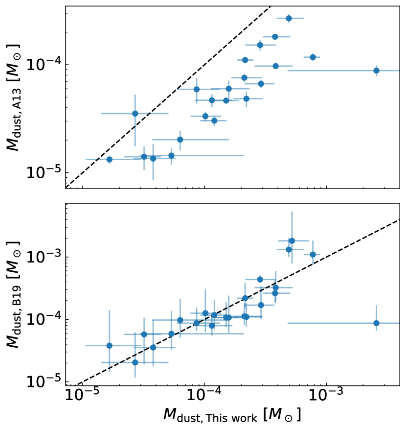
On the other hand, because DIAD solves the temperature and density structure of the disk, the dust masses derived in this study do not require the assumptions of isothermal and/or optically thin emission. The adopted Bayesian approach also accounts for the effect that other parameters have in the uncertainties of disk masses. In Fig. 6 we compare our disk dust mass estimates with those of Andrews et al. (2013) based on 1.3 mm fluxes (after correcting them for the new Gaia DR2 distances), as well as with those of Ballering & Eisner (2019) from radiative transfer models. Our mass values are systematically higher than those from Andrews et al. (2013), with the median being $\sim$3 times higher. In contrast, the comparison with Ballering & Eisner (2019) yields much more compatible results. These authors computed two sets of dust masses using radiative transfer models: Their estimates enforcing a $L_{\rm mm}-R_{\rm disk}$ relation are still $\sim$25 % lower than ours, but their results when not including that relation show a very good agreement with ours (median difference of $\sim$2 %). These comparisons clearly indicate that, as discussed in Ballering & Eisner (2019), dust mass estimates from (sub)mm fluxes are very likely underestimated by factors of a few as a considerable fraction of the emission at these wavelengths remains optically thick. A similar conclusion was also reached by Woitke et al. (2019) when modeling SEDs, gas lines, and spatially resolved observations of disks. These findings imply that results based on disk dust masses measured from (sub)mm fluxes alone should be considered with caution, because they may be reflecting properties other than mass. A full radiative transfer modeling considering the physical structure of the disk is therefore needed to obtain reliable mass estimates.

The higher disk masses found when using full radiative transfer models alleviate the apparent discrepancy between the measured masses of exoplanetary systems and those of protoplanetary disks. Manara et al. (2018) compared dust masses for disks in Lupus and Chamaeleon I derived from ALMA observations at 890 $\mu$m with those of core masses in planets and planetary systems, and found that the core masses were 3-5 times more massive (median value) than the dust disks. Since the disk masses measured in this work are $\sim$3 times higher than those measured with (sub)mm data alone, this could explain the aforementioned discrepancy. Nevertheless, we caution that our sample is still small in size and mostly includes disks without substructures, so we cannot exclude the possibility that a substantial mass reservoir is already locked in planetesimals in these disks.

Finally, we also searched for the $M_{*}-M_{\rm disk}$ relation, which was identified in the past using disk masses derived from (sub)mm fluxes (e.g., Andrews et al. 2013; Pascucci et al. 2016). Recently, Ballering & Eisner (2019) found tentative evidence for such a correlation (at a 2-$\sigma$ confidence level) using their mass estimates from SED fitting when enforcing a $L_{\rm mm}-R_{\rm disk}$. However, given the relatively low significance of the correlation and that the influence of the $L_{\rm mm}-R_{\rm disk}$ relation in the $\chi^{2}$ value had to be introduced in an ad hoc manner, further evidence is required to unambiguously confirm the $M_{*}-M_{\rm disk}$ relation. Using our results and the approach in Andrews et al. (2013) based on the Bayesian analysis of Kelly (2007), we found no evidence of a correlation between these two quantities (see also Fig. 13), possibly due to the small size of our sample. Nevertheless, we note that if (sub)mm fluxes are in fact optically thick, then this previously claimed correlation may not reflect a true connection between $M_{*}$ and $M_{\rm disk}$, and may instead be probing changes the disk structure or dust properties. Disk mass estimates from radiative transfer models accounting for optical depth effects are needed for larger samples of disks to revisit this correlation.

7 Summary

We have used the physically motivated DIAD models to fit the complete SEDs of 23 protoplanetary disks in the Taurus-Auriga star-forming region using a Bayesian framework. This analysis was possible thanks to the vast increase in computational performance achieved by combining these models with artificial neural networks. Our main results are:

• Several of the modeled disks require high viscosities and accretion rates, in contradiction with recent observational estimates of low turbulence in disks. We also derive high levels of dust settling in the sample, which the DIAD models treat independently of the viscosity and can thus be used as another indirect indicator of low turbulence in disks. Combined with theoretical predictions of low ionization levels in most regions in the disk and other observational results, these findings support the idea that disk winds could play an important role in angular momentum transport in disks.

• We find evidence of a population of very compact disks, also in agreement with recent findings of ALMA high-resolution observations.

• The posterior distributions of grain sizes in the disk midplane are largely unconstrained, with only mild evidence of large grains in disks. This suggests that little to no evidence about grain growth can be gained by analyzing SEDs or (sub)mm spectral indices alone.

• The derived disk masses are systematically higher than those obtained using the standard conversion from (sub)mm fluxes, probably because the emission at these wavelengths is still (partially) optically thick. Disk dust masses computed directly from (sub)mm fluxes should therefore be considered with caution. The higher disk masses derived in this study decrease previous tensions between disk mass measurements and those of exoplanetary systems.

Appendix A Effect of different parameters on the SED

Figure 7: Effect of changing different parameters on the SED. Parameters are modified one at a time, the others are fixed to the values described in Sect. A. The bottom right panel also shows the change in the SED produced by varying both the viscosity and accretion rate while keeping their ratio constant.

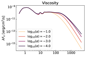
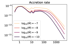
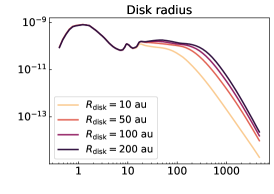
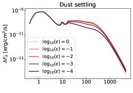
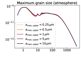
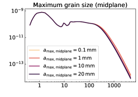
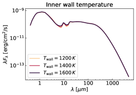
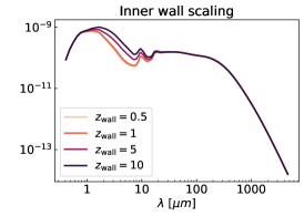
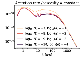
Here we show the impact of different parameters on the SEDs from the DIAD models. The default disk has the following parameters: age=2 Myr and $M_{*}$=0.5 M_⊙ (corresponding to $T_{*}=3725$ K and $R_{*}$=1.5 R_⊙ according to the MIST isochrones used), viscosity parameter $\alpha=10^{-3}$, mass accretion rate $\dot{M}=10^{-8}M_{\odot}$/yr, dust settling $\epsilon=10^{-1}$, disk radius $R_{\rm disk}=$100 AU, inner wall temperature and scaling $T_{\rm wall}$=1400 K and $z_{\rm wall}$=2, grain sizes in the upper layers and midplane $a_{\rm max,upper}=1\,\mu$m and $a_{\rm max,midplane}$=1 mm, and distance $d=100$ pc. Figure. 7 shows how modifying these parameters affects the corresponding SED. We also show the effect of varying both $\alpha$ and $\dot{M}$ while keeping their ratio constant (at $10^{-6}M_{\odot}$/yr) to separate the effects of the individual parameters (accretion luminosity and viscous heating) from their effect on the dust surface density.

Appendix B The artificial neural network

B.1 Architecture of the artificial neural networks

ANNs can have different architectures based on the arrangement of their layers. For our study, we have chosen a feedforward configuration (i.e., the connections between the nodes do not go backward or form cycles). Figs. 8 and  9 show the chosen architectures for the ANNs used to estimate SEDs and disk masses, respectively. These configurations were selected by trial and error by increasing the number of nodes in each layer until the validation error did not improve significantly. Given that this is a regression problem, we used a rectified linear unit function for the activation function.

Figure 8: Architecture of the ANN used to mimic the DIAD models. The input layer (red circles) contains 12 nodes, one per free parameter considered in DIAD. The input layer is connected to two hidden layers (empty circles), with 250 nodes each. Finally, the output layer contains 100 nodes, each being the flux at one of the considered 100 wavelengths. The bias units of the input and hidden layers are also shown.

Figure 9: Architecture of the ANN used to compute disk masses based on the DIAD input parameters. In this case, the disk mass depends on 10 free parameters, which is the number of nodes in the input layer (red circles). The input layer is connected to a single hidden layer (empty circles), with 250 nodes. The output layer has a single node (the disk mass). The bias units of the input and hidden layer are also shown.

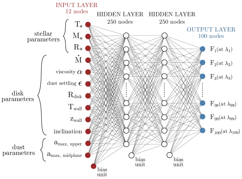
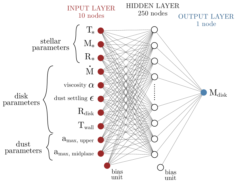
B.2 Generation of the training sample

A sample of DIAD models is needed in order to train the ANN (i.e., to determine the correct weight for each connection). This training sample should cover the desired range of the parameter space. We chose to distribute the DIAD models randomly (although not uniformly) in this parameter space instead of using a grid. This guarantees that each model has a unique value of each parameter (except for grain sizes, which can only have values from a discrete list, see below), maximizing the available information for training. The models were computed as follows:

• Stellar temperature, radius, and mass ($T_{*}$, $R_{*}$, and $M_{*}$): These are the stellar parameters in the DIAD models, and are tightly connected through stellar evolution. We therefore relied on the MIST isochrones (Dotter 2016; Choi et al. 2016; Paxton et al. 2011, 2013, 2015) to avoid sampling non-physical combinations of these parameters. For this purpose, we randomly chose a value for $M_{*}$ between 0.1 and 2.5 $M_{\odot}$ and an age between 0.1 and 10  Myr. We then computed the corresponding $T_{*}$ and $R_{*}$ according to MIST, and added Gaussian noise to these values (with a standard deviation of 250 K and 25 %, of the stellar radius, respectively). If the resulting values met 3000 K $<T_{*}<$ 7000 K, the combination of $T_{*}$, $R_{*}$, and $M_{*}$ was accepted. We note that the only effect of this process is to generate more models in areas consistent with stellar evolution, thus improving the accuracy of the ANN in these regions.

• Mass accretion rate ($\dot{M}$): Typical accretion rates for T Tauri stars are between $10^{-7}-10^{-9}$ $M_{\odot}$/yr, although both higher and lower values are also found (e.g., Ingleby et al. 2013). Therefore, we selected random $\dot{M}$ values in logarithmic scale, ranging from $10^{-10}$ to $10^{-6.5}M_{\odot}$/yr.

• Disk viscosity parameter ($\alpha$): This parameter was explored in logarithmic scale from $10^{-4}$ to 0.1.

• Dust settling ($\epsilon$): We explored this parameter in logarithmic scale from $10^{-4}$ (very settled disk) to 0 (no settling). Values below this range have no impact on the SED (at that value the upper layers of the disk are mostly devoid of dust), and $\epsilon>1$ values have no physical meaning (they correspond to disks with more dust in the upper layers than in the midplane).

• Disk radius ($R_{\rm disk}$): This parameter was explored uniformly from 10 au to 300 au, a broad range covering typical disk size estimates from resolved observations.

• The dust sublimation temperature ($T_{\rm wall}$): A commonly adopted sublimation temperature is 1400 K. Therefore, we uniformly explored temperatures in a 500 K range centered around this value (from 1150 to 1650 K).

• The height of the disk wall ($z_{\rm wall}$): The inner wall may be curved and/or puffed-up due to the vertical structure of the disk (see e.g., Natta et al. 2001; Dullemond & Monnier 2010), which increases its surface area. Since the true shape of the wall is still uncertain, we scaled the wall height by a factor of $z_{\rm wall}$ times the local hydrostatic scale height to account for this uncertainty. $z_{\rm wall}$ was uniformly probed from 0.5 to 15.

• Inclination ($i$): Following the observational distribution of inclinations, $i$ was sampled uniformly in $\cos{(i)}$ space. For inclinations above 70 °, self-extinction from the disk becomes important and small variations of the inclination produce drastic changes in the photospheric emission. This adds a significant complication for training an ANN to accurately predict SEDs with high inclinations. Therefore, we sampled the inclination using the observational distribution from 0 to 70 °, and removed sources with $i\geq 70$ from our sample (see Sect. 3).

• Maximum grain size in the disk atmosphere ($a_{\rm max,upper}$): It is usually assumed that the size distribution of grains in the upper layers of the disk follows that of the ISM, with $a_{\rm max,upper}$ values of 0.25 $\mu$m. We thus randomly sampled from a list of discrete values of $a_{\rm max,upper}$ from 0.25 $\mu$m to 10 $\mu$m to account for the possibility of larger grains in the disk atmosphere that have not settled yet. The list of explored values starts at 0.25 $\mu$m and increases in steps of 0.25 $\mu$m up to 2.5 $\mu$m, then includes 3, 4, 5, and 10 $\mu$m.

• Maximum grain size in the disk midplane ($a_{\rm max,midplane}$): Several studies have found evidence of grain growth in protoplanetary disks, with most sources harboring dust grains of a few mm-cm (e.g., D’Alessio et al. 2006; Ricci et al. 2010a, b; Ribas et al. 2017). Therefore, we considered $a_{\rm max,midplane}$ values from 100 $\mu$m to 2 cm to cover this range. This parameter was also explored in a discrete manner by randomly choosing from a list of discrete values, from 100 $\mu$m to 1 mm in steps of 100 $\mu$m, and from 1 mm to 2 cm in steps of 1 mm.

B.3 ANN training, committees, and accuracies

As mentioned in Section 2.2, we used the multilayer perceptron regressor in the scikit-learn Python package (Pedregosa et al. 2011). Some input parameters of the DIAD models, as well as their outputs, cover several orders of magnitude, and the accretion rate, the alpha viscosity parameter, the dust settling, the SED fluxes, and the disk mass were all trained in logarithmic space. The range of each input and output parameters were re-normalized between 0 and 1 before training.

Figure 10: Evolution of the SME for the training and validation samples during the training of the ANN. The SME decreases rapidly during the first iterations until convergence is reached. Since the training sample used (the DIAD models) do not have noise, no overfitting occurs (no increase is seen in the validation error with increasing iterations).

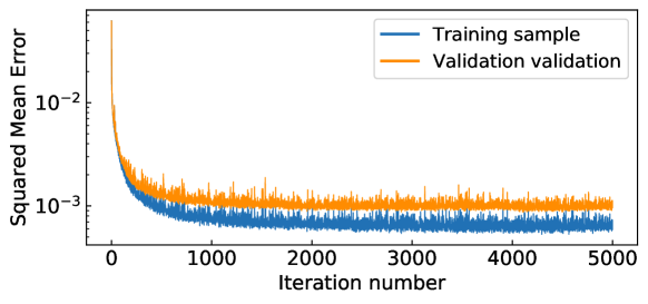
The training was performed with the scikit-learn implementation of the stochastic gradient-based optimizer Adam algorithm (Kingma & Ba 2014). The training sample comprises 70000 DIAD models, and another 17000 are used for validation purposes ($\sim$80% and $\sim$20%, respectively). We trained the ANN for 5000 iterations and monitored the squared mean error (SME) of both the training and validation samples. The ANN with the lowest validation SME was used. The models do not contain any noise (i.e., the same input parameters will always yield the same SED) so we do not expect overfitting to occur. This is confirmed by the approximately constant SME of the validation sample with increasing iterations once convergence has been reached, which in all cases happened before the 5000 iterations used (see Fig. 10).

Training a neural network (almost) never reaches absolute convergence but, instead, it yields weights that are close to their optimal values (e.g., see Bailer-Jones et al. 2002). For this reason, predictions from neural networks include some error. In our case, this implies that the output SED from the ANN is not exactly the same as the SED from the DIAD models given the same input parameters. To mitigate this effect, we trained a total of five different ANNs using the process formerly described, and use them jointly as a committee: The final prediction of the flux at each wavelength is the median value of the predictions from each of the five ANN. This was performed for both the ANN predicting the SED and the one predicting disk masses.

Figure 11: Accuracy of the ANN. For each object in the blind sample (5000 models), we estimated the difference between the SED from DIAD and the SED predicted by the ANN at each wavelength. We then estimated the 68 % (1-$\sigma$), 95 % (2-$\sigma$), and 99.9 % (3-$\sigma$) percentiles. The yellow line corresponds to the median difference between DIAD and the ANN at each wavelength. The bottom plot shows a zoom to the -25 % - 25 % range.

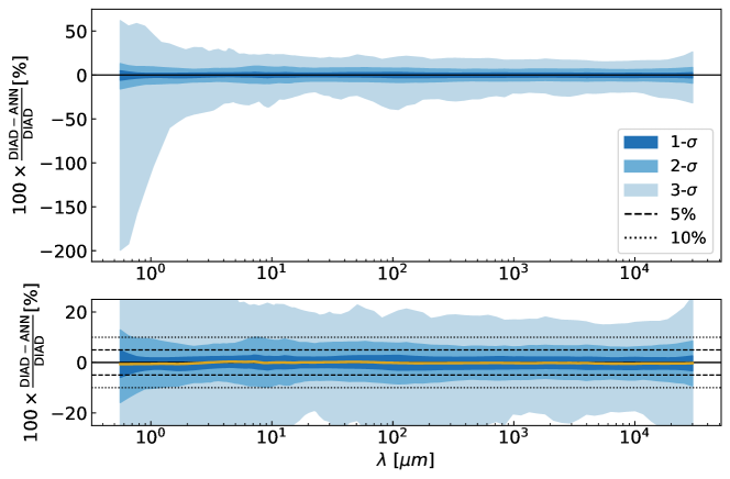
The accuracy of the ANNs was tested with an additional blind sample of 5000 models that were randomly generated following the same procedure as for the training and validation samples. These models were not used during the training. Once the ANN was trained, we used it to predict the SEDs of these 5000 models and estimated the resulting residuals at each wavelength: we found that, in general, 1-$\sigma$ deviations correspond to a 5 % discrepancy between the ANN prediction and the true DIAD model (see Fig. 11), with its median value centered at 0 (i.e., the ANN does not have a tendency to over- or underpredict). At high inclinations, self-extinction of the stellar and inner wall emission by the disk becomes important, producing a strong decrease in the flux at optical and near-IR wavelengths. These changes are extremely sensitive to small variations of the relevant disk parameters (e.g., inclination, settling), and the ANN weights need to be very accurate in order to account for these effects. As a result, the uncertainty at wavelengths $\lesssim$10 $\mu$m increases: while the 1-$\sigma$ and 2-$\sigma$ deviation levels are still within 5 % and 10 %, respectively, the 3-$\sigma$ level reaches up to 200 %. Performing the same process with inclinations $\leq$ 60 °yields a 3-$\sigma$ uncertainty within 50 %, clearly showing that this problem is only important for cases with considerable self-extinction. Since this affects mostly disks that are close to edge-on (which we do not attempt to fit in this study), we do not expect this to have any significant impact on our results. Nevertheless, we adopted a conservative 1-$\sigma$ uncertainty of 10 % in the ANN prediction of the SED. We also used the same procedure to quantify the accuracy of the ANN estimating disk masses, finding a 1-$\sigma$ difference between the ANN prediction and the correct value from DIAD of $<$ 5 %.

Appendix C Priors

C.1 Priors used in this study

Bayesian analysis requires the use of priors that encompass previous knowledge about parameters. The adopted priors in this study are listed in Table 1.

Table 1: Priors used for the Bayesian analysis in this study

Parameter	Prior	[Range] or mean, standard deviation
Age	${\mathcal{U}}$(min, max)	[0.1, 10] Myr
Disk viscosity, $\alpha$	${\mathcal{J}}$(min, max)	[$10^{-4}$, $10^{-1}$]
Accretion rate, $\dot{M}$	${\mathcal{J}}$(min, max)	[$10^{-10}$, $10^{-6.5}$] $M_{\odot}$/yr
Disk radius, $R_{\rm disk}$	${\mathcal{U}}$(min, max)	[10, 300] au
Dust settling, $\epsilon$	${\mathcal{J}}$(min, max)	[$10^{-4}$, 1]
Temperature of inner wall, $T_{\rm wall}$	${\mathcal{N}}$($\mu$, $\sigma$)	$\mu$=1400 K, $\sigma$=50 K
Height of inner wall, $z_{\rm wall}$	${\mathcal{U}}$(min, max)	[0.5, 15]
Inclination, $\cos{(i)}$ (no observational constraint)	${\mathcal{U}}$(min, max)	[0, 70] °
Inclination, $i$ (observational constraint)	${\mathcal{N}}$($\mu$, $\sigma$)	$\mu=i_{\rm observed}$, $\sigma=i_{\rm unc}$
Max. grain size upper layers, $a_{\rm max,upper}$	${\mathcal{J}}$(min, max)	[0.25, 10] $\mu$m
Max. grain size midplane, $a_{\rm max,midplane}$	${\mathcal{J}}$(min, max)	[0.01, 1] cm
Distance, $d$	$\propto d^{2}$(min, max)	[100, 200] pc
Interstellar extinction, $A_{V}$	${\mathcal{U}}$(min, max	[0, 8] mag
Outliers mean, $y_{\rm out}$	${\mathcal{U}}$(min, max)	[$10^{-15}$, $10^{-8}$] $\lambda$Fλ
Outliers standard deviation, $\sigma_{\rm out}$	${\mathcal{U}}$(min, max)	[$10^{-15}$, $10^{-8}$] $\lambda$Fλ
Outliers fraction, $P_{\rm out}$	${\mathcal{U}}$(min, max)	[0, 0.2]

C.2 Origin of observational inclination measurements

Several sources in this work have been observed with high-spatial resolution, which can provide prior information about disk inclinations. Inclination values for BP Tau, CI Tau, DH Tau, DK Tau, DL Tau, DN Tau, DO Tau, DQ Tau, DR Tau, DS Tau, FT Tau, GI Tau, GO Tau, Haro 6-13, HK Tau, HO Tau, HP Tau, IQ Tau, V710 Tau, and V836 Tau were compiled from Long et al. (2019). For CW Tau, we used the inclination derived from continuum observations in Piétu et al. (2014), since it has a smaller uncertainty than the corresponding estimate from CO emission. Inclination values from gas observations in Simon et al. (2017) were used for CX Tau, CY Tau, FM Tau, and FP Tau (in this case, uncertainties derived from the gas emission were smaller than those from the continuum data). Finally, inclination values for FN Tau and DG Tau were compiled from Kudo et al. (2008) and Bacciotti et al. (2018), respectively. No uncertainties are reported for these two objects, and we adopted a value of 10°. In all cases, an additional uncertainty of 3°  was added in quadrature to the ones listed in the literature (or adopted) to account for possible systematics or underestimated uncertainties.

Appendix D Likelihoods

As mentioned in Sect. 4.2.3, we used a likelihood function that includes up to four different terms, namely: a photometric likelihood, a spectroscopic likelihood, a likelihood for the stellar temperature, and a likelihood for the observed parallax (when available). Here we describe each of these terms.

Photometric likelihood: $\mathcal{L}_{\rm phot}$ evaluates the likelihood of the photometric data. Due to their heterogeneity, it is likely that some data do not agree with the overall SEDs for different reasons (e.g., variability, confusion with companions in the case of low-spatial resolution), and we expect some outliers. Therefore, we used a mixture model to include the possibility that a fraction $P_{\rm out}$ of the observations arise from a different (outlier) model: a Normal distribution centered at $y_{\rm out}$ and with a standard deviation of $\sigma_{\rm out}$ (for a description of this method, see Hogg et al. 2010). This adds three additional parameters to the modeling process. While we marginalized over them after the fitting, these parameters also require priors: We chose a uniform prior for $P_{\rm out}$ from 0 to 0.2 (i.e., the maximum number of possible outliers in an SED is 20 %), and uniform priors for $y_{\rm out}$ and $\sigma_{\rm out}$, both of them from $10^{-15}$ to $10^{-8}$ erg/cm²/s based on the ranges of observed flux values ($\sigma_{\rm out}$ was explored in logarithmic space following Hogg et al. 2010). With the adopted mixture model, the likelihood function for photometric data is

$$\mathcal{L}_{\rm phot}=\prod_{i=1}^{N_{\rm phot}}\bigl{(}\mathcal{L}_{\rm SED,i}+\mathcal{L}_{\rm out,i}\bigr{)},$$ (3)

where the index $i$ corresponds to each photometric measurement, and $\mathcal{L}_{\rm SED,i}$ and $\mathcal{L}_{\rm out,i}$ are the likelihoods of a given photometric point arising from the SED model and from the outlier model, respectively. These can be written as

$$\mathcal{L}_{\rm SED,i}=\frac{1-P_{\rm out}}{\sqrt{2\pi[\sigma_{i}^{2}+\sigma_{i,{\rm model}}^{2}]}}\exp{\biggl{(}-\frac{(y_{i}-y_{i,{\rm model}})^{2}}{2[\sigma_{i}^{2}+\sigma_{i,{\rm model}}^{2}]}\biggr{)}}$$ (4)

$$\mathcal{L}_{\rm out,i}=\frac{P_{\rm out}}{\sqrt{2\pi[\sigma_{i}^{2}+\sigma_{\rm out}^{2}]}}\exp{\biggl{(}-\frac{(y_{i}-y_{\rm out})^{2}}{2[\sigma_{i}^{2}+\sigma_{\rm out}^{2}]}\biggr{)}},$$ (5)

where $y_{i}$ and $\sigma_{i}$ are the observed fluxes and the corresponding uncertainties, $y_{i,{\rm model}}$ is the flux predicted by the ANN at the same wavelength, and $\sigma_{i,{\rm model}}=0.1\times y_{i,{\rm model}}$ is the adopted uncertainty for the ANN (10 %).

Spectroscopic likelihood: $\mathcal{L}_{\rm spect}$ evaluates the likelihood of the spectrocopic data. Spitzer/IRS spectra are available for all the objects in the sample, and Herschel/SPIRE spectra also exist for some of them. In this case, we chose the standard likelihood form for Normal uncertainties, and did not account for possible outliers since all the data in the spectra are taken simultaneously. Therefore, the adopted likelihood for the spectra is

$$\mathcal{L}_{\rm spect}=\prod_{i=1}^{N_{\rm spect}}\frac{1}{\sqrt{2\pi[\sigma_{i}^{2}+\sigma_{i,{\rm model}}^{2}]}}\exp{\biggl{(}-\frac{(y_{i}-y_{i,{\rm model}})^{2}}{2[\sigma_{i}^{2}+\sigma_{\rm out}^{2}]}\biggr{)}},$$ (6)

where $y_{i}$, $\sigma_{i}$, $y_{i,{\rm model}}$, and $\sigma_{i,{\rm model}}=0.1\,y_{i,{\rm model}}$ have the same meaning as in the photometric case. Here, $\sigma_{i}$ are the weighted uncertainties of the spectra (see Sect. 4.2.1).

Stellar temperature likelihood: while the fundamental parameters of stellar evolution are age and $M_{*}$, the spectral type/effective temperature of stars is the easiest to measure. For our sample, $T_{*}$ estimates are available through spectroscopic observations (see Sect. 3). Therefore, although $T_{*}$ is not an input parameter of the models, we require that the $T_{*,\rm isochrone}$ value obtained from the MIST isochrones (see step 1 in Sect. 4.1) is compatible with the observed $T_{*}$. For this purpose, we include a term in the likelihood that accounts for the stellar temperature, $\mathcal{L}_{\rm T_{*}}$. Assuming Normal uncertainties for $T_{*}$, this likelihood is

$$\mathcal{L}_{\rm T_{*}}=\frac{1}{\sqrt{2\pi\sigma_{\rm T_{*}}^{2}}}\exp{\biggl{(}-\frac{(T_{*}-T_{*,\rm isochrone})^{2}}{2\sigma_{\rm T_{*}}^{2}}\biggr{)}},$$ (7)

where $T_{*}$ is the adopted stellar temperature from the SpTs in Luhman et al. (2017, see also Section 3), $\sigma_{\rm T_{*}}$ is the uncertainty of this value (set to 100 K, see Sect.3), and $T_{*,\rm isochrone}$ is the temperature predicted by the MIST isochrones based on the input age and $M_{*}$ values for the model.

Parallax likelihood: for most objects in our sample, a parallax estimate is available from the Gaia DR2 catalog. In those cases, we included a term in the likelihood to incorporate this information:

$$\mathcal{L}_{\rm parallax}=\frac{1}{\sqrt{2\pi\sigma_{\varpi}^{2}}}\exp{\biggl{(}-\frac{(\varpi-\varpi_{model})^{2}}{2\sigma_{\varpi}^{2}}\biggr{)}}.$$ (8)

In this expression, $\varpi$ and $\sigma_{\varpi}$ are the observed parallax and its uncertainty, and $\varpi_{model}$ is the parallax corresponding to the model distance. We note that the likelihood is written in terms of parallax instead of distance to account for the fact that parallax uncertainties are not symmetric in distance space. When no parallax measurement exists, this term is not included in the likelihood.

Appendix E Results for individual sources

Table 2 lists modeling results for individual sources for the parameters of interest in Sect. 5.2. We note that these should be considered with caution especially when comparing some of them with observational results, since a direct comparison is not always straightforward: For example, the accretion rate in the disk is not necessarily the same as the accretion rate onto the star (which can be largely variable), and the disk radius is different for different grain sizes due to radial migration whereas our models use one single value.

Table 2: Modeling results for the relevant (non-marginalized) parameters. The reported values correspond to the derived median of each parameter, while uncertainties are computed as 16 % and 84 % percentile levels.

Source	$\alpha$	$\dot{M}$ [$\times 10^{-8}M_{\odot}$/yr]	$R_{\rm disk}$ [au]	$\epsilon$ [$\times 10^{-4}]$	$a_{\rm max,upper}$ [$\mu$m]	$a_{\rm max,midplane}$ [mm]	$M_{\rm disk}$ [$\times 10^{-2}M_{\odot}]$
BP Tau	$0.017_{-0.013}^{+0.006}$	$2.0_{-1.6}^{+0.6}$	$250_{-70}^{+40}$	$1.27_{-0.2}^{+0.59}$	$1.4_{-0.5}^{+3.0}$	$2.4_{-1.5}^{+2.8}$	$1.5_{-0.3}^{+0.4}$
CIDA 7	$0.003_{-0.002}^{+0.005}$	$0.13_{-0.1}^{+0.17}$	$160_{-110}^{+90}$	$80_{-50}^{+170}$	$0.42_{-0.11}^{+0.16}$	$2.7_{-2.0}^{+5.2}$	$0.27_{-0.13}^{+0.24}$
CI Tau	$0.014_{-0.006}^{+0.007}$	$4.0_{-0.9}^{+1.1}$	$160_{-60}^{+90}$	$11_{-5}^{+14}$	$1.3_{-0.3}^{+1.0}$	$0.6_{-0.5}^{+2.4}$	$3.8_{-0.8}^{+1.3}$
CW Tau	$0.06_{-0.02}^{+0.03}$	$10.4_{-2.1}^{+1.8}$	$53_{-15}^{+55}$	$4.6_{-1.8}^{+3.4}$	$5.0_{-1.7}^{+2.6}$	$2_{-2}^{+4}$	$1.1_{-0.3}^{+0.5}$
CX Tau	$0.06_{-0.03}^{+0.02}$	$2.4_{-0.6}^{+0.7}$	$170_{-120}^{+90}$	$2.2_{-0.9}^{+1.9}$	$0.45_{-0.14}^{+0.21}$	$3_{-3}^{+4}$	$0.32_{-0.1}^{+0.12}$
CY Tau	$0.00014_{-0.00003}^{+0.00005}$	$0.042_{-0.009}^{+0.018}$	$260_{-40}^{+30}$	$1.11_{-0.08}^{+0.13}$	$9.2_{-1.1}^{+0.6}$	$0.8_{-0.3}^{+0.6}$	$7.7_{-1.2}^{+1.1}$
DE Tau	$0.0005_{-0.0003}^{+0.0159}$	$0.04_{-0.03}^{+1.56}$	$260_{-60}^{+30}$	$10_{-5}^{+17}$	$5_{-3}^{+2}$	$7.3_{-3.1}^{+1.8}$	$1.0_{-0.2}^{+0.4}$
DG Tau	$0.025_{-0.008}^{+0.01}$	$29.0_{-2.7}^{+1.9}$	$43_{-5}^{+9}$	$2000_{-2000}^{+5000}$	$6.9_{-2.0}^{+1.9}$	$1.0_{-0.8}^{+3.4}$	$4.9_{-1.0}^{+1.7}$
DN Tau	$0.0016_{-0.0012}^{+0.0025}$	$0.4_{-0.3}^{+0.6}$	$230_{-100}^{+50}$	$1.6_{-0.5}^{+0.8}$	$7.6_{-2.1}^{+1.7}$	$3_{-2}^{+3}$	$3.8_{-1.3}^{+1.5}$
DS Tau	$0.019_{-0.009}^{+0.012}$	$1.8_{-0.6}^{+0.8}$	$230_{-80}^{+50}$	$1.4_{-0.3}^{+0.7}$	$1.0_{-0.3}^{+0.8}$	$1.2_{-1.0}^{+2.4}$	$1.2_{-0.3}^{+0.3}$
FM Tau	$0.008_{-0.005}^{+0.006}$	$6.5_{-1.8}^{+1.4}$	$10.3_{-0.2}^{+0.5}$	$1.5_{-0.4}^{+1.5}$	$1.0_{-0.3}^{+0.6}$	$0.5_{-0.3}^{+1.8}$	$0.6_{-0.3}^{+1.0}$
FP Tau	$0.00017_{-0.00006}^{+0.00013}$	$0.08_{-0.04}^{+0.06}$	$170_{-70}^{+80}$	$3.7_{-1.8}^{+3.2}$	$7.7_{-3.1}^{+1.6}$	$0.9_{-0.7}^{+3.1}$	$5.2_{-1.2}^{+2.0}$
FY Tau	$0.0018_{-0.0013}^{+0.0082}$	$0.07_{-0.05}^{+0.24}$	$150_{-90}^{+110}$	$21_{-12}^{+28}$	$6_{-3}^{+2}$	$1.6_{-1.3}^{+4.9}$	$0.38_{-0.12}^{+0.2}$
FZ Tau	$0.03_{-0.02}^{+0.02}$	$11_{-3}^{+4}$	$11.6_{-1.2}^{+3.0}$	$3.0_{-1.5}^{+8.8}$	$3.2_{-1.4}^{+2.7}$	$1.1_{-0.8}^{+4.7}$	$0.5_{-0.2}^{+1.6}$
GI Tau	$0.07_{-0.03}^{+0.02}$	$4.1_{-1.4}^{+1.4}$	$34_{-20}^{+77}$	$9_{-5}^{+11}$	$0.34_{-0.07}^{+0.1}$	$3_{-3}^{+5}$	$0.17_{-0.06}^{+0.14}$
GO Tau	$0.0004_{-0.0003}^{+0.0006}$	$0.07_{-0.04}^{+0.09}$	$190_{-70}^{+70}$	$21_{-10}^{+18}$	$0.64_{-0.16}^{+6.36}$	$0.27_{-0.09}^{+0.22}$	$2.2_{-0.3}^{+0.4}$
Haro 6-13	$0.02_{-0.006}^{+0.009}$	$11.9_{-1.1}^{+1.1}$	$37_{-5}^{+8}$	$600_{-400}^{+800}$	$3.5_{-1.0}^{+2.0}$	$4_{-3}^{+4}$	$2.9_{-0.7}^{+1.0}$
HO Tau	$0.0018_{-0.0012}^{+0.0016}$	$0.24_{-0.15}^{+0.17}$	$220_{-80}^{+60}$	$2.1_{-0.8}^{+1.8}$	$1.5_{-0.5}^{+0.8}$	$1.5_{-1.1}^{+3.2}$	$1.6_{-0.5}^{+0.8}$
HP Tau	$0.0009_{-0.0007}^{+0.0041}$	$11.3_{-1.1}^{+1.4}$	$17.3_{-2.1}^{+2.0}$	$40_{-30}^{+240}$	$1.6_{-0.5}^{+0.7}$	$1.3_{-1.0}^{+3.0}$	$30_{-20}^{+180}$
IQ Tau	$0.0013_{-0.001}^{+0.0113}$	$0.3_{-0.2}^{+2.4}$	$190_{-100}^{+70}$	$10_{-5}^{+9}$	$7.6_{-2.4}^{+1.7}$	$1.3_{-1.0}^{+3.0}$	$2.1_{-0.5}^{+0.8}$
IRAS 04385+2550	$0.039_{-0.016}^{+0.018}$	$12_{-3}^{+3}$	$28_{-7}^{+9}$	$1000_{-700}^{+1200}$	$2.8_{-1.5}^{+2.7}$	$3_{-3}^{+4}$	$0.9_{-0.3}^{+0.5}$
V710 Tau	$0.0008_{-0.0006}^{+0.0018}$	$0.18_{-0.14}^{+0.36}$	$150_{-60}^{+80}$	$2.9_{-1.2}^{+2.4}$	$4_{-3}^{+3}$	$0.27_{-0.13}^{+0.54}$	$2.2_{-0.5}^{+0.8}$
V836 Tau	$0.00021_{-0.00008}^{+0.00026}$	$0.036_{-0.017}^{+0.052}$	$260_{-70}^{+30}$	$1.6_{-0.4}^{+1.0}$	$0.41_{-0.09}^{+0.53}$	$3.3_{-1.9}^{+3.5}$	$2.9_{-0.8}^{+0.8}$

Appendix F Marginalized parameters

Some parameters in our model are either nuisance ones (i.e., the three parameters required to model possible outlier photometric points) or are included to account for our ignorance about their true values and their impact on other parameters. Therefore, their posteriors are not really informative or relevant for our study, and we do not analyze them in detail. These parameters are:

Figure 12: Results for individual sources (top panels) and ensemble distribution (bottom panels) of the marginalized parameters in our study for the sample of 23 modeled disks. The ensembles are produced similarly to the ones in Fig. 5.

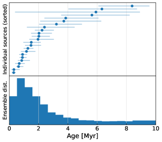
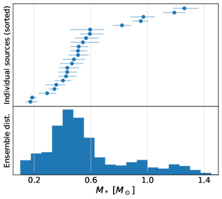
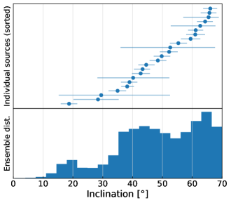
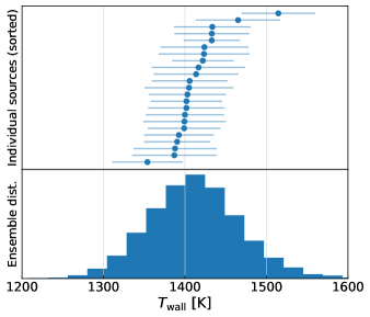
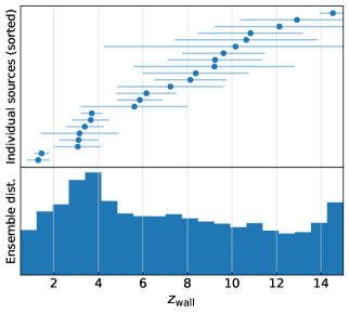
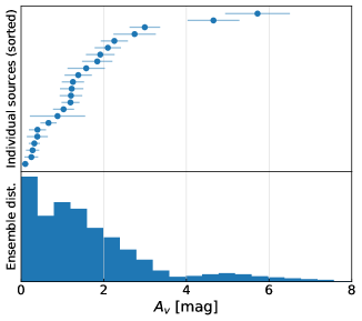
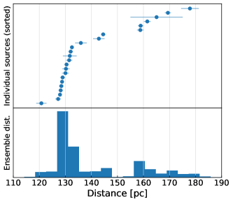
• Stellar parameters (age, $M_{*}$, $T_{*}$, and $R_{*}$): our model contains two star-related parameters (age and $M_{*}$), which are passed to the MIST isochrones to derive consistent $T_{*}$ and $R_{*}$ values. While these are constrained in all cases, we do not expect their values to be truly accurate: this would require a more complete treatment of the photospheric fluxes during the fitting process, that is, the use of high-resolution synthetic spectra and convolutions with the corresponding photometric filters. Instead, the photospheric values in DIAD come from the empirical colors in Pecaut & Mamajek (2013) and are interpolated at intermediate wavelengths when needed. Therefore, the derived stellar parameters are just approximate, and are used for internal consistency of the models and to account for the additional uncertainties they produce in other parameters. Nevertheless, they are compatible with more precise estimates from previous studies using spectroscopic measurements (e.g., Luhman et al. 2017). It is worth noting the resulting distribution for the age, with a clear preference for values$\sim$1-2 Myr and steep but smooth decline toward older ages.

• Inclination ($i$): there is little information about disk inclinations in unresolved photometry, except in the case of edge-on disks (which were excluded from our sample, Sect. 3). In all cases, the posterior distribution of this parameter resembled the prior used, meaning that no useful information was grained during the modeling process.

• The dust sublimation temperature ($T_{\rm wall}$) and scaling of the inner wall of the disk ($z_{\rm wall}$): these two parameters encapsulate our ignorance about the true shape and location of the inner wall. The posterior of $T_{\rm wall}$ resembles the prior used and is still centered around $\sim$1400 K. On the other hand, the scaling factor $z_{\rm wall}$ is required to account for the additional solid angle of the wall because DIAD assumes a flat, vertical wall. This factor is correlated with the inclination, since disks close to face-on will require, in general, a larger $z_{\rm wall}$ value. Overall, the posterior shows that some scaling is required in all cases, thus suggesting that the inner walls are indeed curved and/or puffed-up. However, given the ad hoc weighting of the Spitzer/IRS spectra and the fact that we have not explored different dust compositions (which play a crucial role in the location and temperature of the inner wall), we do not consider the results for $z_{\rm wall}$ to be informative of its true value.

• Distance ($d$): the posterior distributions for the distances are completely dominated by the Gaia DR2 data, as expected: Distances derived from photometric data are much more uncertain and do not improve upon Gaia estimates, so our modeling process does not provide any additional information about this parameter.

• Extinction ($A_{V}$): extinction values are constrained in all cases but, as in the case of the stellar parameters, a precise estimate of this quantity requires a proper convolution of each photometric filter with photospheric models. Therefore, the derived $A_{V}$ values only provide general estimates of extinction values. All sources objects have $A_{V}<6$ mag, in good agreement with other studies (e.g., Andrews et al. 2013).

• Parameters modeling outlier photometric data ($y_{\rm out}$, $\sigma_{\rm out}$, and $P_{\rm out}$): these are the three parameters involved in the outlier rejection model. While the mixture model makes the fitting more robust to possible outliers, these parameters have no physical meaning.

The ensemble posterior distributions for the marginalized parameters are show in Fig. 12.

Appendix G Correlations between $\dot{M}$, $\alpha$, and $M_{\rm disk}$

Figure 13: Comparison of the derived $\dot{M}$, $\alpha$, and $M_{\rm disk}$ values. $\dot{M}$ and $\alpha$ appear clearly correlated, as expected for the $\alpha$-disk prescription. However, $M_{\rm disk}$ does not show strong correlations with these parameters.