Cosmic voids in modified gravity models with massive neutrinos

Abstract

Cosmic voids are progressively emerging as a new viable cosmological probe. Their abundance and density profiles are sensitive to modifications of gravity, as well as to dark energy and neutrinos. The main goal of this work is to investigate the possibility of exploiting cosmic void statistics to disentangle the degeneracies resulting from a proper combination of $f(R)$ modified gravity and neutrino mass. We use N-body simulations to analyse the density profiles and size function of voids traced by both dark matter particles and haloes. We find clear evidence of the enhancement of gravity in $f(R)$ cosmologies in the void density profiles at $z=1$. However, these effects can be almost completely overridden by the presence of massive neutrinos because of their thermal free-streaming. Despite the limited volume of the analysed simulations does not allow us to achieve a statistically relevant abundance of voids larger than $40\ \mathrm{Mpc}/h$, we find that the void size function at high redshifts and for large voids is potentially an effective probe to disentangle these degenerate cosmological models, which is key in the prospective of the upcoming wide field redshift surveys.

1 INTRODUCTION

The Universe has recently entered a phase of accelerated expansion. This revolutionary discovery goes back to more than two decades ago and was originally achieved thanks to distant type Ia supernovae (Riess et al., 1998; Perlmutter et al., 1999; Schmidt et al., 1998). The following observations of the cosmic microwave background anisotropies and large-scale structures have then supported this scenario (e.g. Eisenstein et al., 2005; Komatsu et al., 2011; Bennett et al., 2013; Planck Collaboration et al., 2018), , which is now widely accepted among the scientific community. Nevertheless, the understanding of the physics behind this accelerated expansion remains one of the fundamental open questions in cosmology, and a plethora of theoretical models have been proposed to explain this phenomenon (see e.g. Yoo & Watanabe, 2012, for a review).

The standard paradigm of modern cosmology, the $\Lambda$-cold dark matter ($\Lambda$CDM) model, interprets the accelerating expansion of the Universe as due to the existence of an extra component, named dark energy, contributing to about the $70\%$ of the total energy density of the Universe. In its most trivial description, this component behaves like a fluid with a negative equation of state, which can be straightforwardly described by the cosmological constant $\Lambda$ in the Einstein field equations. Thanks to its simplicity and its concordance with the majority of current cosmological observations, the $\Lambda$CDM model is nowadays the most popular and widespread cosmological model (Shafieloo & Clarkson, 2010; Heavens et al., 2017). However, this scenario has been often questioned, since it clashes with both some theoretical and observational issues. The former concern for instance the coincidence and the fine-tuning problems (Weinberg, 1989; Carroll, 2001; Martin, 2012, but see Bianchi & Rovelli 2010 for an alternative perspective), while the latter are raised in particular by the recent measurements of the Hubble constant, $H_{0}$, together with other well-known anomalies and tensions (see e.g. Bernal et al., 2016; Moresco & Marulli, 2017; Verde et al., 2019, and references therein). Hence, new ideas and different theoretical approaches arose to solve or alleviate these possible fundamental inconsistencies. Among the proposed solutions, some models interpret the dark energy component as a dynamical variable slowly varying with the cosmic time, or as exotic new forms of energy that would cause the observed late time accelerated rate of the Universe (see e.g. Frieman et al., 2008; Wen et al., 2018, and references therein). There are also alternative explanations which involve a modification of General Relativity (GR) in a manner that leads to accelerating solutions. In this class of models the standard GR is supposed to be inadequate on certain cosmological scales, which implies also the introduction of new physical degrees of freedom in the gravitational theory to explain its behaviour on small scales (see e.g. Dolgov & Kawasaki, 2003; Nojiri & Odintsov, 2006; Clifton et al., 2012; Joyce et al., 2015; Ishak, 2019). In particular, Modified Gravity (MG) models tend to closely mimic the effect of the cosmological constant on the expansion history of the Universe. To satisfy the solar system tests and the local high-precision measurements (Le Verrier, 1859; Bertotti et al., 2003; Will, 2005), these models have to introduce a screening mechanism, that basically recovers the predictions of standard GR on small scales (Khoury & Weltman, 2004; Hinterbichler & Khoury, 2010; Brax & Valageas, 2013, 2014). Most viable MG models are quite degenerate at the background level and can produce discernible features only through their effects on structure formation at linear and nonlinear scales. Additionally, it has been recently highlighted the presence of strong observational degeneracies between the effects of some of these models and those including massive neutrinos (He, 2013; Motohashi et al., 2013; Baldi et al., 2014; Wright et al., 2017; Giocoli et al., 2018). Neutrinos are indeed another elusive component of the $\Lambda$CDM cosmology, and although the Standard Model of particle physics assumes they are massless, the evidence of solar neutrino oscillations proved they in fact possess a mass (Becker-Szendy et al., 1992; Fukuda et al., 1998; Ahmed et al., 2004).

In this paper we will investigate the degeneracies emerging from a proper combination of the parameters of the so-called $f(R)$ class of MG models and of the total neutrino mass, $\sum m_{\nu}$. In particular, Baldi et al. (2014) have demonstrated that many standard cosmological statistics, as the nonlinear matter power spectrum, the halo abundance and the halo bias, show a limited discriminating power for some specific combinations of $f(R)$ gravity parameters and neutrino mass values, for which they revealed to be statistically consistent with the $\Lambda$CDM predictions. Our goal is to investigate whether it is possible to disentangle these degenerate cosmological scenarios by exploiting a novel promising cosmological probe, i.e. the cosmic voids, and more precisely their radial profiles and abundances.

Voids are defined as large regions of the Universe with low-density interiors and shallow gravitational potentials. Thanks to these unique features, they constitute excellent laboratories for investigating the implications of MG theories and the presence of massive neutrinos. Indeed, screening mechanisms operate weakly within cosmic voids, making them potentially more affected by the possible deviations from GR (Spolyar et al., 2013; Barreira et al., 2015; Voivodic et al., 2017; Baker et al., 2018; Falck et al., 2018). Furthermore, voids are particularly sensitive to neutrinos (Zeng & White, 1991; Clampitt et al., 2013; Villaescusa-Navarro et al., 2013a; Massara et al., 2015; Banerjee & Dalal, 2016; Hamaus et al., 2017; Schuster et al., 2019; Kreisch et al., 2019; Dvorkin et al., 2019; Wang et al., 2019; Pisani et al., 2019), since their typical sizes span the range of neutrino free-streaming scales and the density fraction of neutrinos is more prominent in these zones compared to those in high-density ones. Both the void density profiles and void abundances have been shown to possess a great potential in constraining cosmological parameters (see e.g. Pisani et al., 2015; Hamaus et al., 2016, 2020; Sahlén et al., 2016; Sahlén & Silk, 2018; Sahlén, 2019; Contarini et al., 2019; Aubert et al., 2020). Void profiles show a characteristic shape that depends on the mean radius of the void sample, and are well reproduced by the functional form provided by Hamaus et al. (2014). Void abundances have been studied by a number of authors (see e.g. Sheth & van de Weygaert, 2004; Jennings et al., 2013; Pisani et al., 2015; Ronconi & Marulli, 2017; Chan et al., 2019; Correa et al., 2020), and have been recently explored in relation to the modifications induced on the void size function by the bias factor of the tracers (Pollina et al., 2016, 2017; Pollina et al., 2019; Ronconi et al., 2019; Contarini et al., 2019; Verza et al., 2019).

In this work we explore the possibility of breaking the degeneracy between MG and neutrino effects by analysing cosmic voids identified by means of the void finder VIDE (Sutter et al., 2015) in the DUSTGRAIN-pathfinder simulations (Giocoli et al., 2018; Hagstotz et al., 2019a), a set of N-body simulations with a volume of $(750\ \mathrm{Mpc}/h)^{3}$, including cosmological models with both $f(R)$ gravity and massive neutrinos. We study voids traced by both the distribution of DM particles and of collapsed haloes, measuring their density profiles and their abundance as a function of void sizes. The latter is then compared to the theoretical model provided by Jennings et al. (2013), and modified to include the effect of the tracer bias (see Ronconi et al., 2019; Contarini et al., 2019). For a proper comparison with the theoretical predictions, the void sample is analysed according to the prescriptions introduced in Ronconi & Marulli (2017).

The paper is structured as follows. In Section 2 we introduce the theoretical context in which this analysis is inserted, summarising some of the fundamental notions needed to understand the effects of $f(R)$ MG and massive neutrinos. Then we present the theoretical model for the void size function, together with the prescriptions required to take into account the modifications induced by the usage of biased tracers to identify the voids. In Section 3 we describe the set of simulations analysed in this work and the methods adopted to build the catalogues of haloes and voids. We also outline the cleaning procedure applied to recover cosmic voids consistently with the assumptions used in their theoretical modelling. In Section 4 we present the results of our analysis, discussing the void density profiles and void abundances, and focusing on their possible exploitation to disentangle the cosmic degeneracies previously introduced. In Section 5 we finally summarise the main conclusions drawn in this paper.

2 THEORETICAL MODELS

This Section presents the fundamental theoretical background on which this work is based. We briefly start by introducing the MG and massive neutrino models characterising the cosmological simulations analysed in this work. Then we present and discuss the theoretical model for the void size function.

2.1 $f(R)$ modified gravity theory

Among the variety of cosmological models proposed to explain the accelerated expansion of the Universe, we consider those alternative theories that imply a deviation from the standard behaviour of gravity by modifying the left hand side of the Einstein’s field equations:

$$R_{\mu\nu}-\frac{1}{2}g_{\mu\nu}R=8\pi GT_{\mu\nu}\,,$$ (1)

in which $R_{\mu\nu}$ is the Ricci curvature tensor, $R$ the Ricci scalar, $g_{\mu\nu}$ the metric tensor, $G$ the Newton’s gravitational constant and $T_{\mu\nu}$ the stress-energy tensor. One of the simplest ways to modify the GR equations is to change the Einstein-Hilbert action, $S$, introducing a function $f$ of the Ricci scalar:

$$S=\int\mathrm{d}^{4}x\sqrt{-g}\ \Big{(}\frac{R+f(R)}{16\pi G}\Big{)}+\mathcal{L}_{m}\,,$$ (2)

where $\mathcal{L}_{m}$ is the Lagrangian density of all matter fields. In this class of MG theories, called $f(R)$ models, GR is recovered by imposing $f$ to be proportional to the cosmological constant $f=-2\Lambda^{\mathrm{GR}}$. An important requirement to be satisfied by the function $f(R)$ is to match the observed $\Lambda$CDM expansion of the Universe on large scales and to evade the solar system constraints at the same time. A valid form of this function, introduced by Hu & Sawicki (2007), is the following:

$$f(R)=-m^{2}\frac{c_{1}\Big{(}\frac{R}{m^{2}}\Big{)}^{n}}{c_{2}\Big{(}\frac{R}{m^{2}}\Big{)}^{n}+1}\,,$$ (3)

where $m^{2}\equiv H_{0}^{2}\Omega_{\mathrm{M}}$ defines the mass scale $m$, while $c_{1}$, $c_{2}$ and $n$ are non-negative free parameters of the model. In particular we refer to the case in which $c_{1}/c_{2}=6\Omega_{\Lambda}/\Omega_{\mathrm{M}}$, where $\Omega_{\Lambda}$ and $\Omega_{\mathrm{M}}$ represent the present vacuum density and matter density parameters, respectively. Under this specific condition the background expansion history is indeed consistent with the one predicted by the $\Lambda$CDM model. Moreover, imposing $c_{2}(R/m^{2})^{n}\gg 1$ the scalar field $f_{R}\equiv df(R)/dR$ can be approximated by:

$$f_{R}\approx-n\frac{c_{1}}{c_{2}^{2}}\bigg{(}\frac{m^{2}}{R}\bigg{)}^{n+1}\,.$$ (4)

In this work we restrict our analysis to the case $n=1$. With this choice the scalar field can in fact be expressed by means of the parameter $c_{2}$ only, and the model at the present epoch can be represented by the parameter $f_{R0}$:

$$f_{R0}\equiv-\frac{1}{c_{2}}\frac{6\Omega_{\Lambda}}{\Omega_{\mathrm{M}}}\bigg{(}\frac{m^{2}}{R_{0}}\bigg{)}^{2}\,,$$ (5)

where $R_{0}$ indicates the background value of the Ricci scalar at the present time. Now we can derive the modified Einstein equations by varying the action defined in Eq. (2) with respect to the metric $g_{\mu\nu}$:

$$f_{R}R_{\mu\nu}-\frac{1}{2}fg_{\mu\nu}-\nabla_{\mu}\nabla_{\nu}f_{R}+g_{\mu\nu}\Box f_{R}=8\pi GT_{\mu\nu}\,,$$ (6)

in which $\nabla$ is the covariant derivative and $\Box$ is the D’Alembert operator defined as $\Box\equiv g^{\mu\nu}\nabla_{\mu}\nabla_{\nu}$. Here $f_{R}$ turns out to be the responsible for the modification of the GR theory and plays the role of a new dynamical scalar degree of freedom. From the trace of Eq. (6) we can obtain the equation of motion for this scalar field:

$$\nabla^{2}\delta f_{R}=\frac{a^{2}}{3}\left[\delta R(f_{R})-8\pi G\delta\rho_{m}\right]\,,$$ (7)

where $a$ is the scale factor of the metric. To obtain the equivalent of the Poisson equation for the scalar metric perturbation ${2\psi=\delta g_{00}/g_{00}}$, we extract the time-time component from Eq. (6):

$$\nabla^{2}\psi=\frac{16\pi G}{3}a^{2}\rho_{m}-\frac{a^{2}}{6}\delta R(f_{R})\,,$$ (8)

assuming small perturbations on a homogeneous background and a slow variation for $f_{R}$ (quasi-static field).

From Eqs. (7) and (8) it is possible to derive the exact solution for the extreme cases $|f_{R0}|\gg|\psi|$ and $|f_{R0}|\ll|\psi|$. It can be demonstrated that, when the field is large, thus in the former case, the Compton wavelength of the scalar field ${\mu^{-1}=(3\ \mathrm{d}f_{R}/\mathrm{d}R)^{1/2}}$ determines the interaction range of an additional fifth force, which can enhance the gravity field up to a factor of $4/3$ for $k\gg\mu$. Standard gravity is instead restored for scales $k\ll\mu$. In the latter case, instead, the value of $f_{R0}$ is small and Eq. (8) can be approximated by the standard Poisson equation, leading to the recovery of GR in regions of high space-time curvature. This is the so-called Chameleon screening mechanism, which has the effect of hiding the additional fifth force on small scales, suppressing its strength inside large matter overdensities. By solving Eq. (7) under the assumption of small perturbations in the homogeneous background, $\delta f_{R}\leq\bar{f_{R}}$, we can obtain the screening condition for an ideal spherical source of mass $M$ causing the fluctuation of the scalar field:

$$|f_{R}|\leq\frac{2}{3}\psi_{N}(r)\,,$$ (9)

where $\psi_{N}=GM/r$ is the Newtonian potential of the overdensity. In this approximation, the enhancement of gravity is carried out only by the distribution of mass outside the radius for which ${\psi_{N}(r)=3/2\ |f_{R}|}$, that constitutes the transition point between the screened and un-screened regimes.

We can now assess valid estimations for the free parameter $f_{R0}$. The case in which $f_{R0}\ll\psi_{N}$ has no relevant cosmological interest since the fifth force is always screened, hence the resulting scenario is indistinguishable from GR even on large scales. On the other hand, for $f_{R0}\gg\psi_{N}$, we would face the implausible situation in which gravity is always enhanced. Therefore the parameter $f_{R0}$ should be settled around the same order of magnitude of the Newtonian potential $\psi_{N}$, that in turn typically shows values in the range ${10^{-5}\leq\psi_{N}\leq 10^{-6}}$.

2.2 Degeneracies with massive neutrinos

Neutrinos are massive particles participating to the total matter content of the Universe and to the growth of cosmic structures. Given their small masses, neutrinos decouple from high relativistic particles at the early stages of the Universe, when their thermal energy drops below their mass. Precision cosmology allows nowadays to put strong constraints on their physics and especially on the sum of their mass eigenstates $m_{\nu}\equiv\sum_{i}m_{v_{i}}$. The total neutrino mass is indeed constrained by several astronomical observations to be ${m_{\nu}\lesssim 0.1-0.3\ \mathrm{eV}}$ (see e.g. Seljak et al., 2006; Riemer-Sørensen et al., 2013; Lu et al., 2015, 2016; Cuesta et al., 2016; Kumar & Nunes, 2016; Yèche et al., 2017; Poulin et al., 2018), and their contribution to the total amount of energy in the Universe at late cosmological epochs can be computed as (Mangano et al., 2005):

$$\Omega_{\nu}\approx\frac{m_{\nu}}{93.14\ h^{2}\mathrm{eV}}\,.$$ (10)

Given their weak interaction cross-section, neutrinos can be considered as a DM component. However, contrary to CDM particles, neutrinos can free-stream from high density perturbations of matter thanks to their high thermal velocity. Indeed we can derive the typical scales travelled by neutrino perturbations, described by the free-streaming length:

$$\lambda_{\mathrm{FS}}(z,m_{v})=a(z)\frac{2\pi}{k_{\mathrm{FS}}}=7.7(1+z)\frac{H_{0}}{H(z)}\bigg{(}\frac{1\mathrm{eV}}{m_{v}}\bigg{)}\ \mathrm{Mpc}/h\,,$$ (11)

where $k_{\mathrm{FS}}$ is the associated free-streaming wavenumber, which during the neutrino non-relativistic transition, $z_{\mathrm{nr}}$, reaches the minimum value (Lesgourgues et al., 2013):

$$k_{\mathrm{FS}}(z_{\mathrm{nr}})\simeq 0.0178\ \bigg{(}\Omega_{\mathrm{M}}\frac{m_{v}}{\mathrm{eV}}\bigg{)}\ h/\mathrm{Mpc}\,.$$ (12)

Therefore modes with $k<k_{\mathrm{FS}}$ evolve as CDM perturbations since neutrino velocities can be neglected, while on small scales ($k\gg k_{\mathrm{FS}}$) free-streaming leads to the slowdown of the neutrino perturbation growth. Besides suppressing the clustering below their thermal free-streaming scale, neutrinos also affect the shape of the matter auto-power spectrum (Brandbyge et al., 2008; Saito et al., 2008, 2009; Brandbyge & Hannestad, 2009, 2010; Agarwal & Feldman, 2011; Wagner et al., 2012), the halo mass function (Brandbyge et al., 2010; Marulli et al., 2011; Villaescusa-Navarro et al., 2013b), the scale-dependent bias (Chiang et al., 2019), the clustering properties of CDM haloes and redshift-space distortions (Viel et al., 2010; Marulli et al., 2011; Villaescusa-Navarro et al., 2014; Castorina et al., 2014, 2015; Zennaro et al., 2018; García-Farieta et al., 2019), and also the number counts and profiles of cosmic voids (see Section 4).

It has been demonstrated that the observable footprints predicted by MG theories are strongly degenerate with the signatures induced by the presence of massive neutrinos. Indeed, the typical range of the fifth force for $f(R)$ models, determined by the Compton wavelength $\mu^{-1}$, can reach a few tens of megaparsecs (see e.g. Cataneo et al., 2015) depending on the value of the parameter $f_{R0}$, and it is comparable with the free-streaming scale of neutrinos, which can be estimated with Eq. (11). The neutrinos free-streaming can have thus a counteractive effect on the enhanced growth of the cosmic structures, causing a compensation on the cosmological statistical variations given by MG theories. This poses a notable challenge for cosmology, since robust methods and different cosmological probes are required to achieve tight constraints on both massive neutrinos and MG, and especially to disentangle their combined effects. In this context, cosmic voids can contribute as key probes, given their peculiar underdense nature and exceptional spatial extension, comparable to the ranges covered by the fifth force of $f(R)$ models and by the neutrino free-streaming, that make them particularly sensitive to both these components.

2.3 The void size function

In the last decade, cosmic voids have demonstrated their potential as cosmological tools. In particular, void profiles and abundances constitute some of the most promising statistics to exploit. While the former has been already exploited to derive extremely tight cosmological constraints (Hamaus et al., 2020; Aubert et al., 2020; Hawken et al., 2020; Nadathur et al., 2020), the latter, also called the void size function, has not been successfully applied to real data yet.

The void size function commonly rely on the theoretical model developed by Sheth & van de Weygaert (2004) (hereafter the SvdW model), which is derived following the same excursion-set approach used to compute the halo mass function (Press & Schechter, 1974; Cole, 1991; Bond et al., 1991; Mo & White, 1996; Sheth & Tormen, 1999; Sheth et al., 2001). Note that, conversely to what happens during the collapse of overdensities (i.e. DM haloes), the possible initial non-sphericity of the underdensity perturbations tends to vanish during the isolated evolution of voids. This suggests that the adoption of a simple spherical expansion model may be accurate enough in describing the void formation (Blumenthal et al., 1992). To find the mathematical expression of the SvdW model it is required to solve a two-barrier problem: one barrier is necessary to account for void formation and merging (voids-in-voids), and the other for void collapse (voids-in-clouds). Indeed, for the formation of a void it is necessary not only to reach a density contrast below a specific barrier $\delta_{v}$, but also to avoid being extinguished by a collapsing overdensity on larger scales, surpassing the threshold $\delta_{c}$. The latter is given by the overdensity case, in which a halo is considered to be formed after its virialisation, that happens when the spherical perturbation reaches a linear density contrast $\delta_{c}\approx 1.69$, for an Einstein-de Sitter (EdS) Universe (Bond et al., 1991). The barrier $\delta_{v}$ was instead commonly fixed at the characteristic value of the shell-crossing phenomenon, since this event is often associated to the void formation (Blumenthal et al., 1992; Sheth & van de Weygaert, 2004; Jennings et al., 2013). From the theoretical point of view, with the excursion-set formalism we consider an initial negative top-hat perturbation and we model it as a set of concentric shells. Since the repulsive force experienced by the internal layers decreases as a function of the radius (Sheth & van de Weygaert, 2004), the inner shells will expand faster than the external ones, surpassing them at the specific density contrast given by $\delta_{v}\approx-2.71$, in linear theory and for an EdS Universe. However, this condition strictly depends on the initial density profile of the underdensity. Considering more physically motivated density profiles than a top-hat perturbation, the shell-crossing unlikely occurs in voids, at least at observable scales (Shandarin, 2011; Abel et al., 2012; Sutter et al., 2014b; Hahn et al., 2015; Verza et al., 2019). This implies that voids can be modelled accurately by adopting the linear theory and that any underdense threshold $\delta_{v}$ can in principle be selected to identify the voids (see Section 3.2).

From the solution of the two-barrier problem in linear theory, SvdW derived the theoretical expression of the void size function, that is the comoving number density of cosmic voids, $n$, as a function of their effective radius, $r^{\mathrm{L}}$:

$$\frac{\mathrm{d}n^{\mathrm{L}}}{\mathrm{d}\ln r^{\mathrm{L}}}=\frac{f_{\ln\sigma}(\sigma)}{V(r^{\mathrm{L}})}\frac{\mathrm{d}\,\ln\sigma^{-1}}{\mathrm{d}\,\ln r^{\mathrm{L}}}\ \text{,}$$ (13)

where $V(r^{\mathrm{L}})$ is the volume of the spherical fluctuation of radius $r^{\mathrm{L}}$ and $f_{\ln\sigma}$ is the fraction of fluctuations destined to become voids, as predicted by the excursion-set theory:

$$f_{\ln\sigma}=2\sum_{j=1}^{\infty}j\pi x^{2}\sin(j\pi\mathcal{D})\exp\biggl{[}-\frac{(j\pi x)^{2}}{2}\biggr{]}\,,$$ (14)

where

$$x\equiv\frac{\mathcal{D}}{|\delta_{v}^{\mathrm{L}}|}\,\sigma\,,$$ (15)

and

$$\mathcal{D}\equiv\frac{|\delta_{v}^{\mathrm{L}}|}{\delta_{c}^{\mathrm{L}}+|\delta_{v}^{\mathrm{L}}|}\,.$$ (16)

In the previous equations, $\sigma$ is the square root of the mass variance, while $\delta_{v}^{\mathrm{L}}$ and $\delta_{c}^{\mathrm{L}}$ are the merging and collapsing barriers previously described, respectively. The quantity $\mathcal{D}$ represents instead the void-and-cloud factor and parametrises the impact of halo formation on the evolving population of voids. To extend this model to the nonlinear regime, SvdW imposed the conservation of the total number of voids during the transition from linearity to nonlinearity. This condition can be achieved introducing a correction factor ${C\propto(1+\delta_{v}^{\mathrm{NL}})^{-1/3}}$ in the void radius:

$$\frac{\mathrm{d}\,n}{\mathrm{d}\,\ln r}\biggr{|}_{\text{SvdW}}=\frac{\mathrm{d}\,n}{\mathrm{d}\,\ln(C\,r)}\biggr{|}_{\text{lin}}\ \text{.}$$ (17)

The downside of this assumption is that it implies a fraction of volume occupied by voids which can exceed the total volume of the Universe. To address this issue, Jennings et al. (2013) proposed a volume conserving model (hereafter the Vdn model), in which the void volume fraction of the Universe is kept fixed in the transition to the nonlinear regime:

$$V(r)\mathrm{d}\,n=V(r^{\mathrm{L}})\mathrm{d}\,n^{\mathrm{L}}\rvert_{r^{\mathrm{L}}=r^{\mathrm{L}}(r)}\,.$$ (18)

With this further prescription, we can finally write down the expression of the void size function according to the Vdn model:

$$\frac{\mathrm{d}\,n}{\mathrm{d}\,\ln r}\biggr{|}_{\text{Vdn}}=\frac{f_{\ln\sigma}(\sigma)}{V(r)}\frac{\mathrm{d}\ln\sigma^{-1}}{\mathrm{d}\,\ln r^{\mathrm{L}}}\biggr{\rvert}_{r^{\mathrm{L}}=r^{\mathrm{L}}(r)}\,.$$ (19)

This model has been applied in different works (Jennings et al., 2013; Ronconi & Marulli, 2017; Ronconi et al., 2019; Contarini et al., 2019; Verza et al., 2019) and its validity in the prediction of void abundances has been largely demonstrated, provided that the analysed sample is prepared through a proper selection and reshaping of the underdensities identified by the algorithm of void finding (see Section 3.2), in order to match the features that characterise the theoretical definition of voids.

According to the Vdn model, voids are defined as spherical and non-overlapping underdensities, identified in the total matter density field and characterised by an internal density contrast given by $\delta_{v}^{\mathrm{L}}$. To compare the model predictions with the measured void abundance it is therefore necessary to model voids according to the theoretical definition given by the Vdn model (Section 3.2 will be dedicated to the description of this modelling). Nevertheless, since the theoretical model of the void size function is formulated in linear theory, the density contrast used to resize the voids in a nonlinear framework, $\delta_{v}^{\mathrm{NL}}$, has to be converted properly to be used in the model. For this purpose, we exploit the fitting formula provided by Bernardeau (1994) to convert the underdense threshold:

$$\delta_{v}^{\mathrm{L}}=\mathcal{C}\,\bigl{[}1-(1+\delta_{v}^{\mathrm{NL}})^{-1/\mathcal{C}}\bigr{]}\ ,\ \text{with }\mathcal{C}=1.594\,,$$ (20)

which has been demonstrated to be especially accurate for the underdense regions.

Dealing with biased tracers, $\delta_{v}^{\mathrm{NL}}$ has to be converted to take into account the effect of the tracer bias on the void density profiles. Contarini et al. (2019) have demonstrated that the relation between the DM density contrast inside cosmic voids, $\delta_{v,\mathrm{DM}}$, and the corresponding threshold value in tracer distribution, $\delta_{v,\mathrm{tr}}$, can be modelled with a linear relation $\mathcal{F}$, depending only on the large scale effective bias $b_{\mathrm{eff}}$:

$$\delta^{\mathrm{NL}}_{v,\mathrm{DM}}=\frac{\delta^{\mathrm{NL}}_{v,\mathrm{tr}}}{\mathcal{F}(b_{\mathrm{eff}})}\,.$$ (21)

While the meaning and the estimation of the linear function $\mathcal{F}$ will be addressed in Section 4.3, the computation of the large-scale linear bias $b_{\mathrm{eff}}$ from the tracer two-point correlation function will be not discussed in this paper, since it is estimated performing the same Bayesian statistical analysis described in details in Appendix A of Contarini et al. (2019) (see also Marulli et al., 2013, 2018).

Finally, we underline that not only the void size function, but also $b_{\mathrm{eff}}$ depends on the presence of the fifth force and massive neutrinos. They are indeed both strongly correlated to the growth of cosmic structures, which is in turn influenced by modification of gravity and neutrino thermal free-streaming. Therefore the rescaling of the underdensity threshold $\delta^{\mathrm{NL}}_{v,\mathrm{tr}}$ by means of the large-scale effective bias can lead to degenerate effects on the resulting void abundance. A rigorous study of the interplay between these effects on the size function of voids identified using different types of matter tracers is left to future works.

3 PREPARATION OF THE MOCK DATA SAMPLES

In this Section we first present the N-body simulations analysed in this work. Then we describe the method applied to obtain the DM halo samples from DM particle catalogues. In the end we focus on the algorithms of void finding and cleaning.

3.1 The DUSTGRAIN-pathfinder simulations

In this work we use a subset of the cosmological N-body simulations suite called DUSTGRAIN-pathfinder (Dark Universe Simulations to Test GRAvity In the presence of Neutrinos). These simulations have been specifically designed with the aim of investigating the degeneracies between $f(R)$ gravity models and massive neutrinos, and have been recently exploited in different papers finalised to the study of possible methods to disentangle these cosmic degeneracies, that is exploiting weak-lensing (Giocoli et al., 2018; Peel et al., 2018) and clustering statistics (García-Farieta et al., 2019), investigating the massive haloes’ abundance (Hagstotz et al., 2019a), the large-scale velocity field (Hagstotz et al., 2019b), and exploring machine learning techniques (Peel et al., 2019; Merten et al., 2019). The DUSTGRAIN-pathfinder simulations have been carried out using MG-GADGET, a code based on an updated version of GADGET2 (Springel, 2005) developed by Puchwein et al. (2013) to include $f(R)$ gravity models. This code has then been combined with the particle-based implementation described in Viel et al. (2010) to include the effects of massive neutrinos.

The DUSTGRAIN-pathfinder simulations follow the evolution of an ensemble of $(2\times)768^{3}$ particles of DM (and massive neutrinos) within a periodic cosmological box of $750\ \mathrm{Mpc}/h$ per side. In the reference $\Lambda$CDM simulation (i.e. the one characterised by GR and $m_{\nu}=0$) the DM particle mass is equal to $m^{p}_{\mathrm{CDM}}=8.1\times 10^{10}\ \mathrm{M_{\odot}}/h$ and the gravitational softening is set to $\epsilon_{g}=25\ \mathrm{kpc}/h$, corresponding to about $1/40$ of the mean inter-particle separation. The cosmological parameters assumed in these simulations are consistent with the Planck 2015 constraints (see Planck Collaboration et al. (2016)) $\Omega_{\mathrm{M}}=\Omega_{\mathrm{CDM}}+\Omega_{\mathrm{b}}+\Omega_{\nu}=0.31345$, $\Omega_{\Lambda}=0.68655$, $h=0.6731$, $\mathcal{A}_{s}=2.199\times 10^{-9}$, $n_{s}=0.9658$, which give for the $\Lambda$CDM case an amplitude of linear density fluctuations smoothed on a scale of $8\ \mathrm{Mpc}/h$ equal to $\sigma_{8}=0.842$. The remaining set of simulations is created to sample the joint $f(R)-m_{\nu}$ parameter space. The $|f_{R0}|$ parameter assumes the values in the range $[10^{-6}\text{-}10^{-4}]$, while $m_{\nu}$ belongs to the range $[0\text{-}0.3]\ \mathrm{eV}$. All the parameters characterising the simulations considered in this paper are reported in Table 1. Note that the total $\Omega_{\mathrm{M}}$ (including neutrinos) is kept fixed to compare the density power spectrum between cosmologies with and without neutrinos. This results in equal positions of the peak of the power spectrum and ensures that the spectra are identical in the long-wavelength limit. For a more detailed description of the DUSTGRAIN-pathfinder simulations see Giocoli et al. (2018) and Hagstotz et al. (2019a).

Table 1: Summary of the main numerical and cosmological parameters related to the subset of the DUSTGRAIN-pathfinder simulations considered in this work. These simulations are carried out in a volume of $(750\ \mathrm{Mpc}/h)^{3}$ and are composed by $768^{3}$ CDM particles for the $\Lambda$CDM, fR4, fR5 and fR6 models, with the addition of as many massive neutrino particles for the non-$\Lambda$CDM cases. The third column provides the value of the modified gravity parameter $f_{R0}$, while the fourth column the neutrino mass $m_{\nu}$. The other columns provide $\Omega_{\mathrm{CDM}}$ and $\Omega_{\nu}$, that are the CDM and neutrino density parameters respectively, and the CDM and neutrino particle masses $m^{p}_{\mathrm{CDM}}$ and $m^{p}_{\nu}$. The value in the last column is the $\sigma_{8}$ parameter, which corresponds to the linear power normalisation computed at $z=0$.

Simulation name	Gravity model	$f_{R0}$	$m_{\nu}$ [eV]	$\Omega_{\rm CDM}$	$\Omega_{\nu}$	$m^{p}_{\rm CDM}$ [M${}_{\odot}/h$]	$m^{p}_{\nu}$ [M${}_{\odot}/h$]	$\sigma_{8}$
$\Lambda$CDM	GR	–	0	0.31345	0	$8.1\times 10^{10}$	0	$0.842$
fR4	$f(R)$	$-1\times 10^{-4}$	0	0.31345	0	$8.1\times 10^{10}$	0	$0.963$
fR4_0.3eV	$f(R)$	$-1\times 10^{-4}$	0.3	0.30630	0.00715	$7.92\times 10^{10}$	$1.85\times 10^{9}$	$0.887$
fR5	$f(R)$	$-1\times 10^{-5}$	0	0.31345	0	$8.1\times 10^{10}$	0	$0.898$
fR5_0.1eV	$f(R)$	$-1\times 10^{-5}$	0.1	0.31107	0.00238	$8.04\times 10^{10}$	$6.16\times 10^{8}$	$0.872$
fR5_0.15eV	$f(R)$	$-1\times 10^{-5}$	0.15	0.30987	0.00358	$8.01\times 10^{10}$	$9.25\times 10^{8}$	$0.859$
fR6	$f(R)$	$-1\times 10^{-6}$	0	0.31345	0	$8.1\times 10^{10}$	0	$0.856$
fR6_0.06eV	$f(R)$	$-1\times 10^{-6}$	0.06	0.31202	0.00143	$8.07\times 10^{10}$	$3.7\times 10^{8}$	$0.842$
fR6_0.1eV	$f(R)$	$-1\times 10^{-6}$	0.1	0.31107	0.00238	$8.04\times 10^{10}$	$6.16\times 10^{8}$	$0.831$

Among all the comoving snapshots available for this project, we select the ones at the redshifts $z=0,0.5,1,2$, considering only CDM particles also in the case of simulations containing massive neutrinos, though this assumption does not have a major impact on the resulting halo catalogues (see e.g. Villaescusa-Navarro et al., 2013b, 2014; Castorina et al., 2014; Lazeyras et al., 2020). In the following analyses concerning voids in the DM density fields, we apply a subsampling factor to DM particles to reduce the computational time, keeping the $25\%$ of the original particle sample. The collapsed DM structures have been identified for each snapshot, as described in Despali et al. (2016). In particular, the halo catalogues have been obtained by applying the Denhf algorithm (Tormen et al., 2004; Giocoli et al., 2008) to the DM particle sample, finding DM haloes as gravitationally bound structures, without including sub-haloes. When running Denhf, we identify virialised and bound gravitational spherical structures centred on the densest particles. Their virial radius, $R_{\mathrm{c}}$, and viral mass, $M_{\mathrm{c}}$, are defined by the relation:

$$\frac{4}{3}\pi R_{c}^{3}\delta_{\mathrm{c}}\rho_{\mathrm{crit}}=M_{\mathrm{c}}\,,$$ (22)

where $\rho_{\mathrm{crit}}\equiv 3H^{2}/8\pi G$ represents the critical density of the Universe and $\delta_{\mathrm{c}}$ is fixed to $200$ or $500$. In this work we have employed 200c halo catalogues only, thus those derived imposing $\delta_{c}=200$, except for the comparison test shown in Figure 6. The 500c haloes, identified with $\delta_{c}=500$, are indeed rarer objects and their sparsity does not allow to identify a sufficiently large sample of cosmic voids. Moreover, we reject the haloes with a number of embedded DM particles less than $30$, in order to keep only statistically relevant objects and to avoid contamination by spurious density fluctuations. This mass cut corresponds to $M_{\textrm{min}}=2.43\ \mathrm{M_{\odot}}/h$ for the $\Lambda$CDM case, and has been chosen to select a complete and, at the same time, dense enough sample of DM haloes, which is fundamental for identifying a statistically significant number of cosmic voids. The effect of this assumption has been investigated by repeating the analysis with different low mass selections, with the requirement of having a good agreement between the measured effective bias of DM haloes (see Section 2.3) and the theoretical predictions, which we compute using the Tinker et al. (2010) model convolved with the halo mass function of the simulations (see e.g. Eq. A$6$ in Appendix A of Contarini et al. 2019).

Two of the most important characteristics of the employed DM halo catalogues are the volume and the spatial resolution. The sample volume settles indeed the statistical relevance of the measured void abundance and affects the probability of finding large voids, while the spatial resolution determines the smallest scales at which the void number counts are not affected by numerical incompleteness. It is therefore fundamental to compare these quantities with those of the upcoming wide field surveys like the ESA Euclid mission (Laureijs et al., 2011; Amendola et al., 2018), the NASA space mission Wide Field Infrared Survey Telescope (WFIRST) (Green et al., 2012) and the Vera C. Rubin Observatory LSST (LSST Dark Energy Science Collaboration, 2012), in order to put our results into the context of a future application with real data catalogues. At first, with a volume of about $0.42\ (\mathrm{Gpc}/h)^{3}$, the DUSTGRAIN-pathfinder simulations allow the identification of a relatively small sample of voids. This volume can be easily compared to the one of WFIRST, Euclid and LSST, that will cover about $17\ (\mathrm{Gpc}/h)^{3}$, $44\ (\mathrm{Gpc}/h)^{3}$ and $154\ (\mathrm{Gpc}/h)^{3}$, respectively. Considering these volumes (two of which that are more than $100$ times larger than the simulation volume considered in this work), we expect that the uncertainties related to the void statistics presented in this paper will decrease dramatically considering void samples extracted from future real galaxy catalogues. In particular, the Poissonian errors associated to both the stacked density profiles (see Section 4.1) and void size functions (see Section 4.3) will be reduced of a factor proportional to the square root of the increasing of the volume size, hence allowing to achieve a precision more than $10$ times better.

Finally, the DM halo catalogues extracted from the DUSTGRAIN-pathfinder $\Lambda$CDM simulations are characterised by a mean particle separation (MPS) between $8.7$ and $12.4\ \mathrm{Mpc}/h$, for $z=0$ and $z=2$ respectively. These values are indeed of the same order of the expected MPS for the Euclid spectroscopic survey that, with a sky area of $\sim 15000\ \mathrm{deg}^{2}$, will sample over $50$ million of H$\alpha$ galaxies, reaching a spatial resolution of about $10\ \mathrm{Mpc}/h$. The predictions for the spatial resolution of the WFIRST survey are even more encouraging, thanks to the $20$ million H$\alpha$ galaxies that are expected to be detected in the redshift range $1.05<z<2$, sampled over a sky area of $\sim 2400\ \mathrm{deg}^{2}$. Considering instead the LSST photometric galaxy surveys, the MPS of the samples would drop to $\sim 3\ \mathrm{Mpc}/h$, though with a dramatic decreasing of the redshift accuracy.

We can therefore expect that the methodology presented in this paper will gain statistical relevance when applied to the data of the upcoming surveys.

3.2 Void finding and cleaning

In this work we identify cosmic voids by means of VIDE (Sutter et al., 2015), a public toolkit which implements an enhanced version of the void detection code ZOBOV (Neyrinck, 2008). Belonging to the class of algorithms based on geometrical criteria, VIDE searches for local minima in a three-dimensional density field, reconstructed from the tracer positions via the Voronoi tesselation. Then it groups nearby Voronoi cells into zones, merging the adjacent ones to form voids. This procedure makes use of a watershed algorithm, that allows the addition of adjacent zones to a void only if the density of the ridge between them is less than $0.2$ times the mean particle density. The resulting catalogue is constituted of a nested hierarchy of voids, with no assumption about their shapes. Void centres are defined as the volume-weighted barycentre, $\overline{X}$, of the $N$ Voronoi cells that define the void:

$$\overline{X}=\frac{\sum_{i=1}^{N}{\overline{x}_{i}V_{i}}}{\sum_{i=1}^{N}{V_{i}}}\textrm{ ,}$$ (23)

where $\overline{x}_{i}$ are the coordinates of the $i$-th tracer belonging to that void, and $V_{i}$ the volume of its associated Voronoi cell. The effective void radius, $r_{v}$, is instead calculated from the total volume of the void, $V_{v}$, defined as the radius of a sphere having the same volume:

$$V_{v}\equiv\sum_{i=1}^{N}{V_{i}}=\frac{4\pi}{3}r_{v}^{3}\textrm{ .}$$ (24)

We run VIDE on both the DM particle and DM halo distributions, building a void catalogue for each of the cosmological simulations and redshift considered in this work (see Section 3.1).

Figure 1: Visual representation of the voids identified in the DM distribution of the DUSTGRAIN-pathfinder simulations. We show a slice of $20\ \mathrm{Mpc}/h$ of the central part of the simulation box at $z=0$, for each of the cosmological scenarios analysed in this work. The DM particles are displayed in light blue, while the DM haloes have colours from orange to yellow, the latter indicating the more massive ones. The yellow circles with a darker interior represent the voids obtained after the application of the cleaner procedure to the void catalogues previously built by applying the VIDE algorithm.

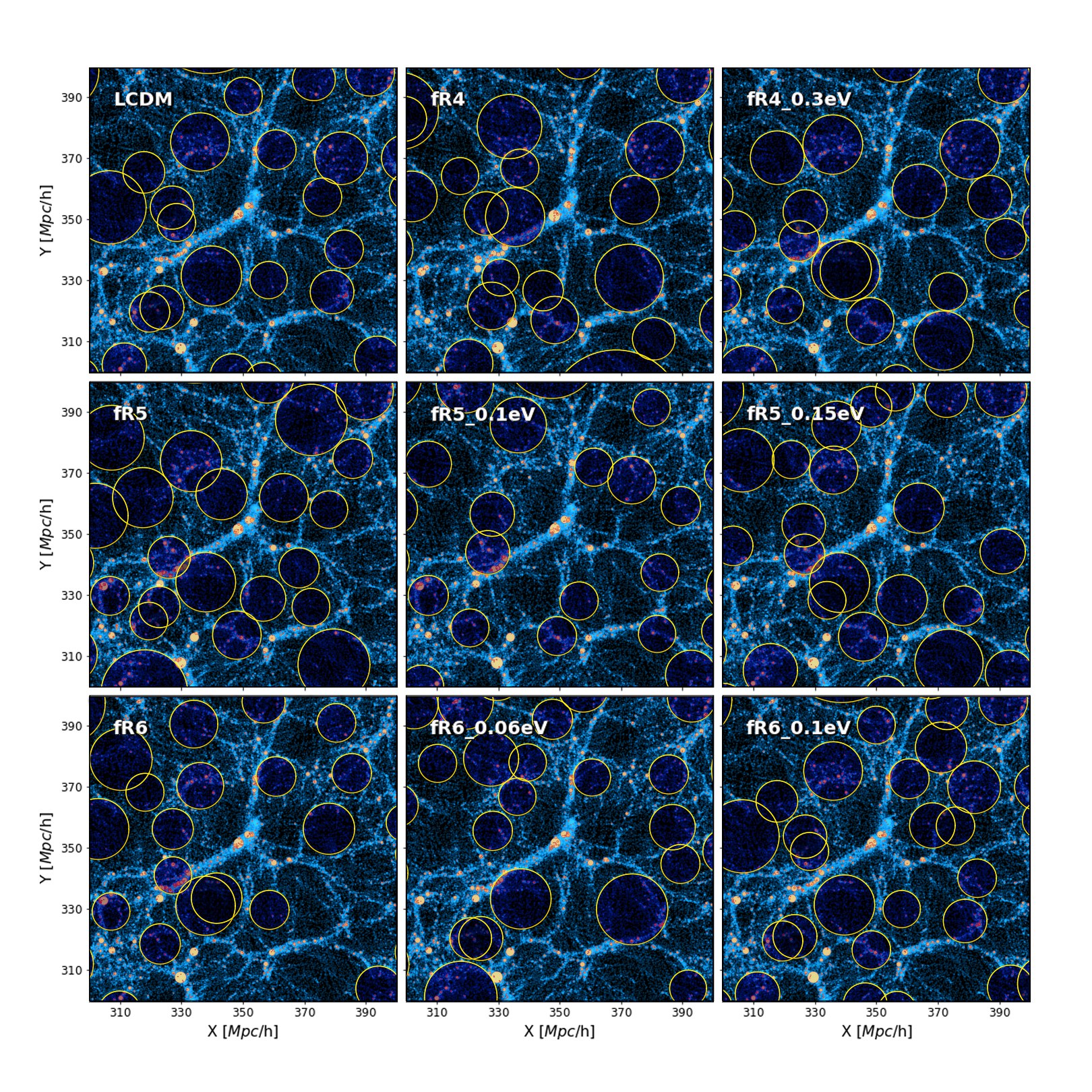
However, cosmic voids identified by VIDE do not satisfy all the assumptions adopted in the theoretical model of the void size function (see Section 2.3). Indeed, according to the definition used in this analysis, voids are spherical non-overlapping regions, centred in density depths of the density field, embedding a fixed density contrast. Therefore we apply a cleaning procedure aimed at aligning the objects included in the void catalogue with the definition of cosmic voids assumed in the Vdn model. This type of procedure was proposed for the first time in Jennings et al. (2013), where it was applied to void catalogues built with ZOBOV, to verify the validity of the methodology using unbiased tracers. In this work, we apply to the VIDE void catalogues an improved version of the algorithm developed by Ronconi & Marulli (2017). As described in the aforementioned paper, this algorithm is structured in three steps, designed to select and reshape the detected underdensities to match the definition used to develop the theoretical model of the void size function. In particular, in the first step the algorithm rejects the cases of voids-in-voids and voids-in-clouds from the input void catalogue, together with the underdensities having a radius outside a spatial range selected by the user. Then, in the second step, it resizes the radius of each void to a specific value $R_{\mathrm{eff}}$, enclosing a given value of the density contrast. Lastly, during the third step the code checks for pairs of overlapping voids, removing the ones with the higher central density. All these steps are independent of the assumed cosmology and of the specific employed void finder. For a more detailed description see Ronconi & Marulli (2017); Ronconi et al. (2019); Contarini et al. (2019).

At the end of the cleaning procedure, the initial void catalogue built with VIDE is pruned of spurious voids, and consists of properly rescaled underdensities following the definition adopted in the Vdn model. Therefore our void catalogues turn out to be composed by non-overlapping spherical objects of radius $R_{\mathrm{eff}}$, characterised by an internal density contrast $\delta^{\mathrm{NL}}_{v}$. As previously mentioned, this value can be fixed to any reasonable threshold, as far as it is both low enough to identify cosmic depressions and high enough to sample zones spatially resolved in the matter distribution. Whatever is the value selected to resize voids, this threshold has to be properly converted using Eq. (20), with a previous rescaling by means of Eq. (21) in the case of biased tracers, and then inserted in Eq. (19) to compute the Vdn model and predict the void abundance of the sample. With this prescription, the theoretical model will be set up to predict the abundance of voids with different depth, according to the threshold selected to rescale the underdensities. However, even if the agreement between the theoretical and the measured void size function is kept for every selection of the threshold $\delta_{v}^{\mathrm{NL}}$, the statistical relevance of the results can depend on this choice. Indeed, choosing a particularly low underdensity threshold (e.g. $\delta_{v}^{\mathrm{NL}}=-0.9$), the scaling algorithm will rescale void towards very small radii, in order to reach this spherical density contrast. This rescaling will cause the leak of void counts due to the increase of small voids that will be discarded during the subsequent exclusion of underdensities with radius belonging to poorly sampled regions, selected according to the MPS of the tracers. Analogously, choosing an underdensity threshold particularly high (e.g. $\delta_{v}^{\mathrm{NL}}=-0.5$) the final sample will be composed by larger rescaled voids, that will be rejected more frequently during the cleaning procedure because of their greater propensity of overlapping, causing also in this case the decreasing of void number counts.

To clean the catalogues of voids identified in the DM halo distribution, we fix the threshold $\delta^{\mathrm{NL}}_{v,\mathrm{tr}}$ at the value $-0.7$, following the choice made in Contarini et al. (2019). Indeed, although voids are shallower depressions at earlier cosmic times, the bias dependence in the $\delta^{\mathrm{NL}}_{v,\mathrm{DM}}$ threshold makes the values high enough to be reached also by voids at high redshifts. On the contrary, dealing with voids in the DM particle distribution, the value $\delta^{\mathrm{NL}}_{v,\mathrm{DM}}=-0.7$ is less appropriate to identify cosmic underdensities. Indeed, only few and very deep voids could be rescaled to enclose such a low density contrast at high redshifts. Since the choice of the threshold does not affect the validity of the predictions of the Vdn model, we decided to use higher density contrasts to clean voids at earlier epochs, adopting different thresholds depending on the redshift of the DM catalogues, using the growth factor $D$ to rescale the nonlinear density contrast required in the cleaning algorithm:

$$\delta_{v,\mathrm{DM}}(z)=-0.8\,\bigg{(}\frac{D(z)}{D(z=0)}\bigg{)}^{2}\textrm{ .}$$ (25)

Fixing the cosmological parameters to those of the $\Lambda$CDM simulations, we obtain the following values: ${\delta_{v,\mathrm{DM}}(z=0)}=-0.80$, ${\delta_{v,\mathrm{DM}}(z=0.5)}=-0.70$, ${\delta_{v,\mathrm{DM}}(z=1)}=-0.62$ and ${\delta_{v,\mathrm{DM}}(z=2)}=-0.52$. It is important to highlight, once again, that the matching between the measured void abundance and the predictions of the Vdn model is not affected by the specific choice of the underdensity threshold. As far as the same value is used to reshape voids and is also inserted, after the conversion in its linear counterpart, in Eq. (19), the results will be in agreement with the model predictions. Therefore the reader should not be misled by the fact that the cleaning procedure is, in this case, cosmology dependent. The usage of the growth factor is just a convenient prescription to select an effective threshold, depending on the redshift of the sample, and does not introduce any cosmology-driven bias. The increasing of the underdensity threshold with the redshift is performed to enlarge the sample of voids and reduce the shot noise. However, it is important to point out that this choice can affect the purity of the void catalogue since these voids are characterised by shallower internal density contrasts and are therefore more prone to be spurious. We also tested different values of the threshold, finding consistent outcomes, as it also has been proved in previous works (Ronconi et al., 2019; Contarini et al., 2019; Verza et al., 2019). Among the tested thresholds, we selected the most effective ones to maximise the signal and reduce the noise associated to the measured void abundances. In particular, we aimed at obtaining a total number of voids that was as large as possible, taking into account the spatial limit given by the numerical incompleteness affecting the void size function (see also Sections 4.2 and 4.3).

Figure 1 shows the voids identified in the distribution of DM particles at $z=0$, obtained following the cleaning procedure described in this section. For each cosmological model, we report the central regions of the simulation box, indicating the spherical underdensities selected in this work with circles traced within a slice of $20\ \mathrm{Mpc}/h$ along the Z-axis. Any apparent overlapping between voids is a visual effect caused by the projection on the plane. As expected, the denser zones made up by filaments are rejected from the selection. Some empty regions result not identified as voids, due to the superimposition with other underdensities not displayed in the figure. It is also interesting to note that the selected sample of voids is different depending on the cosmological scenario, even if the underlying distribution of matter looks remarkably similar, which does not depend on the cleaning procedure, as we verified.

Figure 2: Density contrast profiles computed in shells around the centres of cosmic voids, identified with VIDE in the distribution of DM particles. The results are displayed for each cosmological model at redshifts $z=0,0.5,1,2$. We report in the left plot the profiles measured considering the $\Lambda$CDM, fR4 and fR4_0.3eV simulations. These profiles are so similar that the markers with which they are represented result superimposed. However, the differences between them are highlighted in the residuals reported in each sub-panel, computed with respect to the $\Lambda$CDM case, in units of the errors associated to the profiles computed in the non-standard cosmologies. The latter are represented as a shaded region in the plots. In this case, given the high number of profiles, this uncertainty is so small to be represented with a simple line between the data points. To highlight the deviations from the $\Lambda$CDM void profiles, we show in the sub-panels in the two most-right columns only the residuals obtained with the other models analysed in this work: fR5 and fR6 MG models, with and without massive neutrinos.

4 Results

In this Section we present the main results obtained in this work. We first show the void density profiles traced by the DM particles and by the DM haloes, analysing the differences emerging between the profiles computed in $f(R)$ gravity and massive neutrino cosmologies and the ones of the $\Lambda$CDM case. Then we focus our analysis on the study of the void size function. We compare the measured void abundance with the theoretical predictions of the Vdn model in different cosmologies, using voids identified both in the DM and in the biased tracer distribution, searching for the most efficient methodology to disentangle the cosmic degeneracies between MG and neutrino effects.

4.1 Void profiles

Void profiles have been analysed in different works and their study has demonstrated not only to be promising to derive cosmological constraints (see e.g. Paz et al., 2013; Ricciardelli et al., 2014; Pisani et al., 2014; Nadathur & Hotchkiss, 2015a; Nadathur et al., 2016; Hamaus et al., 2020; Aubert et al., 2020), but also to be useful to understand the overall assembly of the cosmic structures in filaments and walls (Cai et al., 2014; Hamaus et al., 2014; Padilla et al., 2016; Massara & Sheth, 2018). We compute the stacked void density profiles by measuring the density contrast in shells around void centres. In particular, we calculate the mean of the density profiles computed between $0.3$ and $3$ times the effective radius $R_{\mathrm{eff}}$, rescaling then each profile by its correspondent void effective radius. For this specific analysis we make use of the void catalogues obtained directly with VIDE, without applying the cleaning algorithm described in Section 3.2. This is due to the fact that the cleaning procedure is aimed at shaping voids according to the theoretical model of the void size function, and it is not particularly suitable for the study of the stacked void profiles. Indeed, using our cleaning prescriptions, the sample of voids is considerably reduced in number because of the removal of the voids-in-voids, voids-in-clouds and of the overlapping cases. Moreover, with the cleaning algorithm we rescale the void radii to match a specific density contrast, whereas in the study of the stacked density profiles we aim at modelling voids to enhance the self-similarity between their shapes. Indeed, the VIDE void catalogues are composed by a hierarchy of voids separated by high density walls, and the effective radius assigned to each void is, by construction, in proximity to the so-called compensation wall. These voids are therefore characterised by the same shape and their stacking allows to sharpen their peculiar features, as the progressive emptying of the underdense internal parts and the formation of the compensation wall over the cosmic time.

Figure 3: As Figure 2, but for the cosmic voids identified with VIDE in the distribution of DM haloes with $\delta_{c}=200c$.

We start analysing the profiles computed in the DM particle distribution, considering only voids with radii included in the range $[5\text{-}7]$ times the MPS, which corresponds to $1.55\ \mathrm{Mpc}/h$, for all the sub-sampled catalogues. This range covers the central parts of the interval on which we perform the analysis of the abundance of voids in the DM density field presented in the following Section 4.2: the lower limit is given by the spatial resolution of the sample, while the upper limit is chosen to include a sufficient number of voids with large radii. Since the shape of the density profiles depends on the mean radius of the void sample (Hamaus et al., 2014), we avoid to select a wider range of sizes to prevent an excessive mixing of different density profiles during the operation of average.

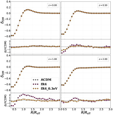
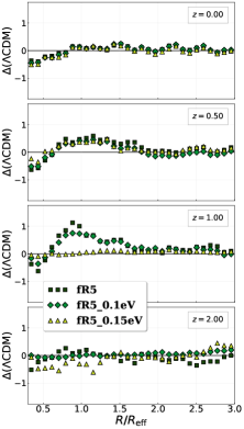
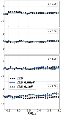
In Figure 2 we show the stacked profiles of voids in the DM field at different redshifts, for the $9$ cosmological models considered in this analysis. In the left plot we report the results obtained with the $\Lambda$CDM simulations, compared to those with MG models characterised by $f_{R0}=-10^{-4}$, with and without massive neutrinos with $m_{\nu}=0.3\ \mathrm{eV}$ (namely, fR4 and fR4_0.3eV). The density profiles in different cosmologies appear very similar, at all redshifts. We note that the central zones become deeper with cosmic time, while the compensation wall grows and turns denser, as already verified in different works (see e.g. Hamaus et al., 2014; Massara et al., 2015; Pollina et al., 2016). Differences among the cosmological models can be better appreciated by looking at the residuals, displayed in the lower sub-panels. Here we compute the difference between the mean density contrast measured in the fR4 or fR4_0.3eV simulations and the one measured in the $\Lambda$CDM simulations, divided by the errors associated to the former. The errors are evaluated as the standard deviation of all the profiles considered for each simulation, divided by the square root of their number. The most significant variation arises around $z=1$, where the fR4 model shows an increase of the mean density in close proximity to the compensation wall and a lowering near the void centres. This is in agreement with the expected effect of enhancing the growth of structures in MG, that accelerates the process of void formation and evolution. The presence of emptier voids and steeper voids profiles has indeed already been observed and predicted by different authors who studied the behaviour of the fifth force in voids in Chameleon models (see e.g. Martino & Sheth, 2009; Clampitt et al., 2013; Perico et al., 2019). Nevertheless, these differences are almost completely cancelled by the effect of the neutrino thermal free-streaming, that slows the evolution of voids and smooths the void density profiles (see also Massara et al., 2015), nullifying the possibility of disentangling the degeneracy between these models. In the right panels of Figure 2 we present the normalised residuals obtained by comparing the density profiles measured using the remaining models to the ones of the $\Lambda$CDM simulation. Note that the y-range is shrunk compared to the previous plot for the sake of clarity. Also in the case of fR5 models, the most evident deviations from the $\Lambda$CDM profiles appear around $z=1$, and they also tend to vanish in the presence of massive neutrinos. The effect is even milder in fR6 models, and statistically indistinguishable, at least with the current simulations.

In order to investigate possible trends related to the void mean size, we repeated the same analysis dividing the stacked void profiles into different bins of effective radii. We do not report the results of this analysis since we did not find any clear different behaviour in the profiles computed with the $\Lambda$CDM cosmology compared to the other models, at the same mean radii. Minor differences appear only for voids with large radii at $z=2$, where an early formation of the compensation wall is revealed in the profiles measured in MG simulations without massive neutrinos. Larger voids manifest also a slightly deeper profiles at ${z=0}$ in the very central regions of the voids, which is reduced by the presence of massive neutrinos. These results are not surprising given that larger voids are subject to a faster evolution compared to the smaller ones. Nevertheless, these deviations do not show a significance higher than $2\sigma$, for all the redshifts and distances from the void centres considered.

Figure 4: Measured and theoretical void size function computed for the $\Lambda$CDM, fR4 and fR4_0.3eV models, at redshifts $z=0,0.5,1,2$. The measured void abundances for each cosmological model are represented by different markers and colours, as described in the label. The errorbars are Poissonian uncertainties on the void counts. The predictions are instead displayed as lines with different colours and styles, according to the model to which they refer. In the bottom sub-panel of each of the $4$ plots are reported the residuals calculated as the difference from the $\Lambda$CDM Vdn model divided by the value of the latter, for both the measured and the predicted void abundance.

Figure 5: Measured and theoretical void size function computed at redshifts $z=0,0.5,1,2$ for the models fR5, fR5_0.1eV, fR5_0.15eV (left panels) and fR6, fR6_0.06eV, fR6_0.1eV (right panels). The description of these plots is analogous to the one reported in the caption of Figure 4.

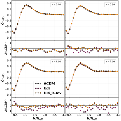
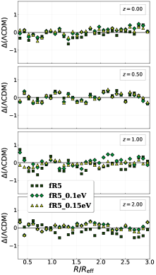
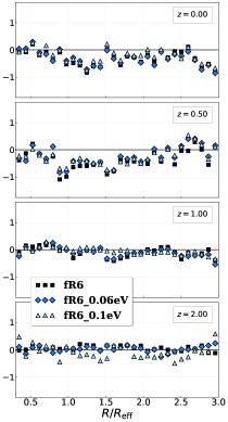
Now we present the same analysis performed on void density profiles measured in the distribution of DM haloes with $\delta_{c}=200$. In this case we consider voids with radii in the range $[2\text{-}5]\times\mathrm{MPS}$ of the $\Lambda$CDM simulation tracers, with $\mathrm{MPS}=8.67\ \mathrm{Mpc}/h$. The choice of this interval of radii is motivated by the same reasons behind the previous analysis of DM void profiles. We report the results of this analysis in Figure 3. In the left panel we present the density profiles for the $\Lambda$CDM, fR4 and fR4_0.3eV models, while in the right panels we show the residuals computed for the set of 6 simulations of the fR5 and fR6 models, with and without massive neutrinos. The residuals are computed as the difference between the profiles measured in non-standard cosmological models and the ones measured in the $\Lambda$CDM cosmology, divided by the uncertainty associated to the former. Compared to the stacked density profiles traced by DM particles, the profiles obtained using DM haloes result steeper and the compensation wall is clearly well developed also at early epochs, reaching more positive values of density contrast (in agreement with the results obtained by Massara et al., 2015). However, in this case the data are noisier because of the decreasing of void statistics, and it is hard to distinguish any significant trend. Since we expect to find the strongest deviations in the most extreme MG models, we focus on the density profiles computed using the simulations with ${f_{R0}=-10^{-4}}$ and $m_{\nu}=0.3\ \mathrm{eV}$. Looking at the residuals shown in the left panel of Figure 3 it is possible to note a slight trend of the fR4 profiles towards lower values of the density contrast, which is almost completely cancelled by the effect of massive neutrinos, especially at high redshifts. The origin of these deviations is the shift of the mean radii of voids identified in MG scenarios by biased tracers. Indeed, being these voids more evolved due to the effect of the enhanced gravity, their average radii result larger. In turn, as demonstrated by Hamaus et al. (2014), the density profiles computed with larger voids have shallower interiors and lower density contrast values in the outer parts. We also tested the subdivision of the sample in different bins of void radii, but the increase of the noise does not allow us to discern any characteristic behaviour associated with voids of different sizes. We can conclude that the degeneracies between the considered models cannot be disentangled by the analysis of the void stacked profiles carried on in this paper, especially making use of DM haloes as tracers of the matter distribution. Nevertheless, we underline that larger simulations could lead to slightly different results, since they would provide better void statistics and smaller errors, possibly allowing us to disentangle the models.

4.2 Void abundance in the DM field

Equipped with the theoretical models delineated in Section 2.3, we can now focus on the study of the abundance of cosmic voids as a function of their effective radius. In this analysis we compare the measured void size function with the predictions of the Vdn model, making use of samples of voids identified in the DM particle distribution. The primary goal of this study is the validation of the methodology with unbiased tracers, which allows us to perform a precise comparison between data and models, thanks to the statistically large sample of detected voids and the absence of the uncertainties related to the measure of the tracer bias. The application of the method to real data would be currently infeasible due to the difficulty of reconstructing the DM density field and the low capability of surveys to detect a population of voids with sizes comparable to the ones considered in the following analysis.

We use the simulations with different $f_{R0}$ parameters and neutrino masses to build the catalogues of voids, exploiting the cleaning algorithm described in Section 3.2. To minimise the effect due to the spatial resolution of the simulations, we apply the conservative choice of rejecting voids with radii smaller than $5.5\ \mathrm{Mpc}/h$, corresponding to about $3.5\times\mathrm{MPS}$. When dealing with voids traced by the DM distribution, no bias prescription is required to rescale void radii. The Vdn model has indeed been demonstrated to successfully predict the abundance of voids identified using unbiased matter distributions in standard $\Lambda$CDM scenarios (Jennings et al., 2013; Ronconi & Marulli, 2017; Ronconi et al., 2019). To include in the theoretical model the variations caused by MG and massive neutrinos on the void size function, we make use of MGCAMB (Zhao et al., 2009; Hojjati et al., 2011; Zucca et al., 2019), a modified version of the public Einstein-Boltzmann solver CAMB (Lewis et al., 2000), which computes the linear power spectrum for a number of alternative cosmological scenarios, including the Hu & Sawicki $f(R)$ model. Since we need to rescale the mass variance at different redshifts, we have to multiply its value at $z=0$ by the normalised growth factor $D(z)/D(z=0)$. We derive the latter by means of MGCAMB, computing the square root of the power spectra ratio $P(z)/P(z=0)$, evaluated on the scales of interest for our analysis.

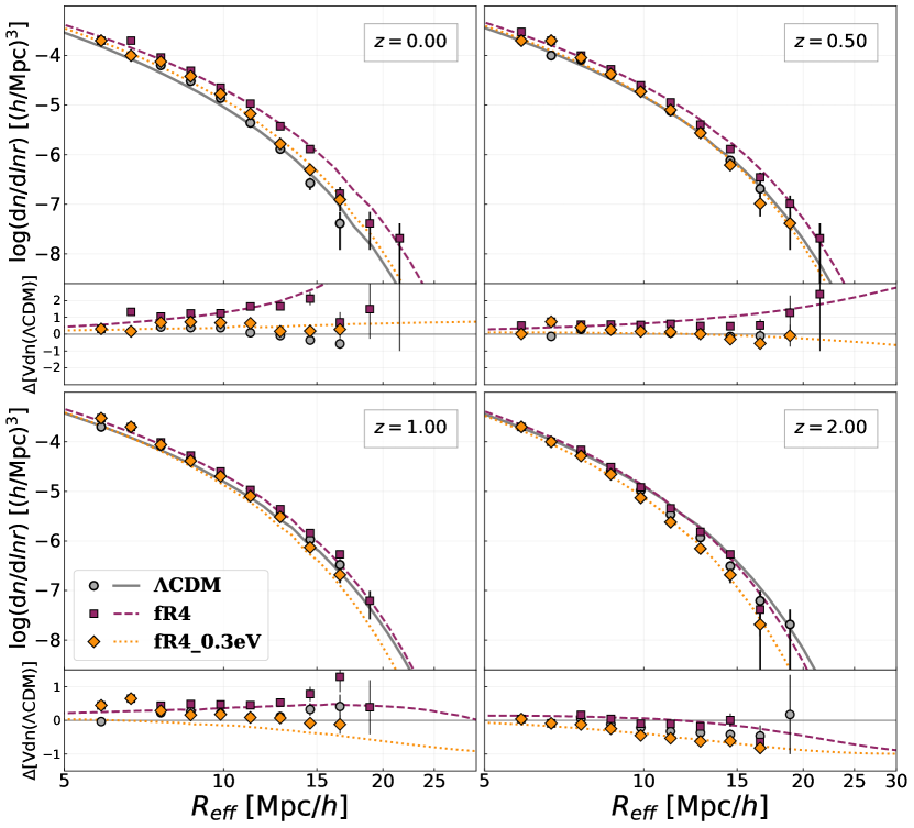
In Figure 4 we show the results for the $\Lambda$CDM, fR4 and fR4_0.3eV models at redshift $z=0,0.5,1,2$. The measured void abundance is represented by different colours and markers for each cosmology, while the corresponding Vdn model is indicated by a line of the same colour. The overall trend of the void size functions measured in the simulations is well reproduced by the models. We considered Poissonian errors, thus the uncertainty on the void counts might be slightly underestimated. In the bottom panels we report the residuals evaluated with respect to the Vdn model computed for $\Lambda$CDM case. In particular, the residuals are calculated as the difference between the measured void abundance and the corresponding predicted one for a given model and the theoretical value of the $\Lambda$CDM void size function at the same radius, divided by the latter. As expected, at low redshifts the fR4 model predicts a larger number of voids with larger sizes. The modification of gravity induces indeed a faster formation and evolution of cosmic structures, including cosmic voids. Figure 5 shows the results of the analysis performed for the remaining cosmological models, given by the set of simulations with ${f_{R0}=-10^{-5}}$ and ${f_{R0}=-10^{-6}}$. Also in these cases, the predictions of the Vdn model computed with MGCAMG are fully consistent with the measured void abundance. The deviations from the $\Lambda$CDM model are weaker in these cases, given the lower values of the $f_{R0}$ parameter. As expected, the departure from the $\Lambda$CDM model are the more severe the stronger is the intensity of the fifth force, resulting more evident for large voids, in agreement to what found by Clampitt et al. (2013) and Voivodic et al. (2017). It is interesting to note that, despite at low redshifts the effect of massive neutrinos is effective in bringing the void size function towards the one computed in $\Lambda$CDM, this trend starts to revert at higher redshifts. In particular, it is evident that at $z=2$ the presence of massive neutrinos makes the fR4_0.3eV void size function to depart from the $\Lambda$CDM one, causing a weakening of the growth of structures, more evident for voids with larger radii. This is a clear hint of the possibility of disentangling the degeneracies between the standard $\Lambda$CDM cosmology and MG with massive neutrino models. However, to achieve this task, it is required to explore the void abundance at high redshifts and in wide areas, in order to collect a sufficiently high number of large voids.

4.3 Void abundance in biased tracer field

The study of the size function of voids identified in a biased tracer distribution is certainly a fundamental step towards its future cosmological exploitation. Many efforts have been made in recent years to understand the effect of a biasing factor on the modelling of cosmic voids (see e.g. Furlanetto & Piran, 2006; Sutter et al., 2014a; Nadathur & Hotchkiss, 2015b; Ronconi et al., 2019; Verza et al., 2019). As anticipated in Section 2.3, Contarini et al. (2019) have introduced a parametrisation of the threshold $\delta_{v}$ of the Vdn model to properly take into account the variations on the void abundance caused by the usage of biased tracers to define voids. The function $\mathcal{F}$, introduced in Eq. (21), is used to convert the tracer bias computed on large scales, $b_{\mathrm{eff}}$, to its corresponding value computed inside cosmic voids. Since the excursion-set theory considers voids identified in the DM distribution, we need to expand the radii of the spherical voids predicted by the Vdn model in order to reach the same density contrast fixed during the cleaning procedure (see Section 3.2). To do this, we have to follow the spherical density profiles of voids and search for the multiplicative factor required to convert the density contrast computed in the DM field to the one measured in the biased tracer distribution, at the punctual distance $R_{\mathrm{eff}}$ from the void centres. This is the same technique described in details in Contarini et al. (2019), aimed at computing the value of $b_{\mathrm{punct}}$, defined therefore as

$$b_{\mathrm{punct}}\equiv\frac{\delta_{v,\mathrm{tr}}(R=R_{\mathrm{eff}})}{\delta_{v,\mathrm{DM}}(R=R_{\mathrm{eff}})}\textrm{ .}$$ (26)

The latter is measured using the mean spherical density profiles and represents the bias of the tracers inside cosmic underdensities. Being this value hardly obtainable in real data catalogues, a conversion is required to calculate it from the measure of $b_{\mathrm{eff}}$. In Contarini et al. (2019) a linear function $\mathcal{F}(b_{\mathrm{eff}})$ has been calibrated by fitting the values of $b_{\mathrm{eff}}$ and $b_{\mathrm{punct}}$ computed at different redshifts, using Friends-of-Friends (FoF) halo catalogues extracted from the CoDECS simulations (Baldi, 2012). In this work we apply the same procedure using the catalogues described in Section 3.1, in particular those characterised by the $\Lambda$CDM cosmology. We consider both the halo catalogues obtained by applying the Denhf algorithm with $\delta_{c}=200$ (200c hereafter) and $\delta_{c}=500$ (500c hereafter) to make a comparison between the relations calibrated with halo samples identified by means of different methods.

Figure 6: Linear relations between $b_{\mathrm{eff}}$ and $b_{\mathrm{punct}}$, calibrated using different halo catalogues for the standard $\Lambda$CDM scenario. The different markers show the data obtained in this work using 200c (in orange) and 500c (in violet) haloes at $z=0,0.5,1,2$. The fitted relations are shown by solid lines and the corresponding relations are represented in orange and violet for 200c and 500c, respectively. The dashed grey line represents the linear function calibrated in a previous work (Contarini et al., 2019), using FoF haloes, extracted from the CoDECS simulations. The uncertainties related to the best-fit models are reported as shaded regions around each linear relation.

Figure 7: Linear relations between $b_{\mathrm{eff}}$ and $b_{\mathrm{punct}}$, calibrated by means of 200c halo catalogues in different cosmological models. The different markers show the data obtained using the values computed for the $\Lambda$CDM (in magenta), fR4 (in blue), fR5 (in green) and fR6 (in yellow) models at $z=0,0.5,1,2$. The best-fit linear models are represented by solid lines with the same colours of the correspondent markers, while their uncertainties are reported as shaded areas around these lines.

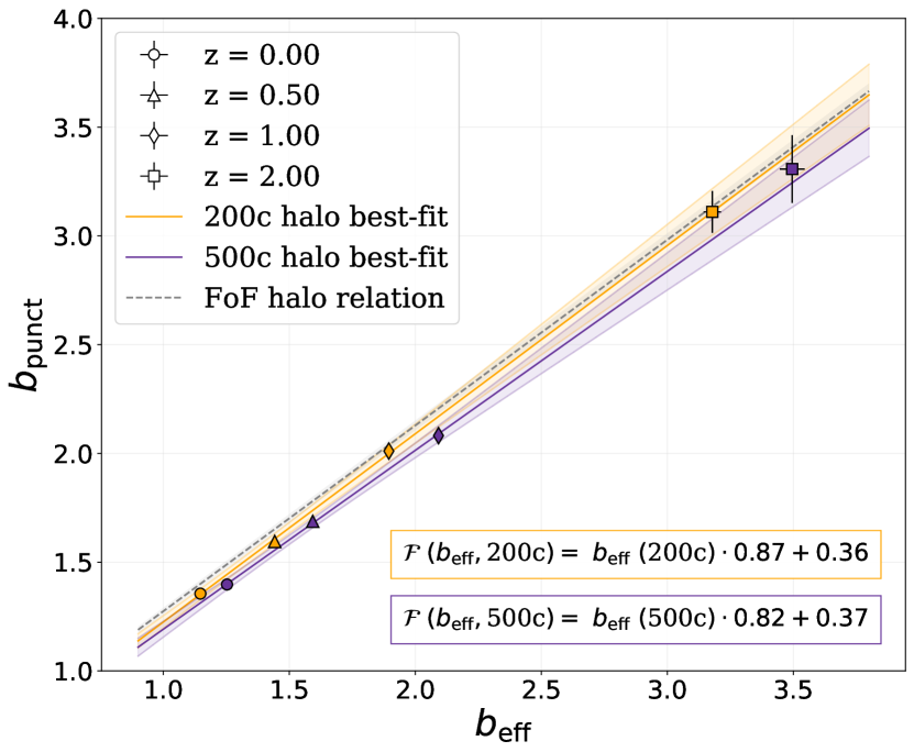
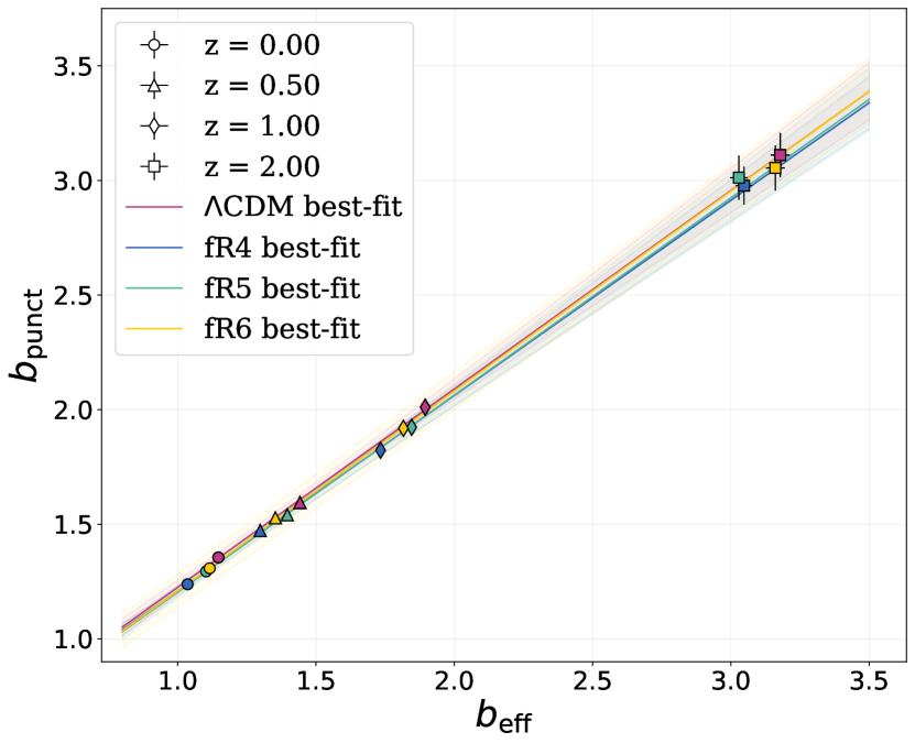
Figure 6 shows the results of this analysis. The new linear relations obtained by fitting the value of $b_{\mathrm{punct}}$ as a function of $b_{\mathrm{eff}}$ at $z=0,0.5,1,2$ are represented with different colours for the 200c and 500c haloes. The fit obtained in Contarini et al. (2019) is also displayed as reference. We note that going from FoF to 200c and 500c haloes, the objects we are considering become more compact and denser. This results in a departure from the bisector of the plane $b_{\mathrm{eff}}$-$b_{\mathrm{punct}}$, representing the relation for matter tracers with an identical behaviour of the bias factor on all the regions of the density field. We find the following results from the fitting of the data at different redshifts:

$$\mathcal{F}(b_{\mathrm{eff}})=(0.87\pm 0.02)\,b_{\mathrm{eff}}+(0.36\pm 0.03)\,,\text{ for 200c}$$ (27)

and

$$\mathcal{F}(b_{\mathrm{eff}})=(0.82\pm 0.02)\,b_{\mathrm{eff}}+(0.37\pm 0.02)\,,\text{ for 500c .}$$ (28)

The linear function $\mathcal{F}$ shows a lowering of the slope related to the increase of the central density selection. We can conclude that the relation required to convert the large-scale effective bias has a slight dependence on the selection criteria applied to define the mass tracers, and that it has therefore to be calibrated according to the type of objects used to identify the voids.

Figure 8: Values of $b_{\mathrm{eff}}$ and $b_{\mathrm{punct}}$ measured using 200c haloes at ${z=0,0.5,1,2}$, for all the cosmological models analysed. The colorbar on the right reports the colours associated to each cosmological model. The black line indicates the linear relation obtained by fitting the $\Lambda$CDM data only, while the shaded grey region shows its associated uncertainty.

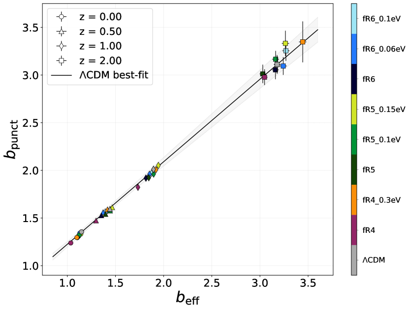
We test also the possible dependence of the function $\mathcal{F}$ on the cosmological model. In Figure 7 we report the linear relations found using the 200c haloes to compute both the values of $b_{\mathrm{eff}}$ and $b_{\mathrm{punct}}$ of the $\Lambda$CDM, fR4, fR5 and fR6 models. In this case, considering tracers with the same mass selection, the $\mathcal{F}$ relation obtained for the $\Lambda$CDM case results statistically indistinguishable from the ones computed for non-standard cosmological scenarios. We finally test the universality of the $\mathcal{F}$ relation analysing also the models with massive neutrinos, comparing the values of $b_{\mathrm{eff}}$ and $b_{\mathrm{punct}}$ measured for these scenarios using 200c haloes with those previously shown. As displayed in Figure 8, the linear relation calibrated with the $\Lambda$CDM model is fully consistent with the data obtained for all analysed cosmological scenarios. For this reason, in the following analysis we will apply the calibration obtained for the $\Lambda$CDM standard scenario to obtain the theoretical void size function for every cosmological model, that is assuming that the $\mathcal{F}$ relation is universal, for a specific type of tracers. In the last part of this Section we make use of the 200c halo catalogues only, since the higher number of tracers and the lower bias factor ease the identification of voids. However, we tested the validity of the following methods considering also the 500c haloes as tracers, finding consistent, though less precise, results.

After obtaining the linear function $\mathcal{F}$ from the analysis of both the DM particle and 200c halo density distribution, we can now use the coefficients shown in Eq. (27) to convert the threshold $\delta_{v,\mathrm{tr}}^{\mathrm{NL}}=-0.7$. This density contrast is used during the cleaning procedure of voids identified in the DM halo field and has to be properly converted to take into account the effect of the bias factor on the theoretical void size function. To this purpose, we first apply Eq. (21) to obtain the nonlinear density contrast in the DM distribution. Then we evaluate its corresponding value in linear theory by means of Eq. (20), inserting this quantity in the theoretical expression of the Vdn model. We repeat this method to compute the theoretical void size function for each cosmological scenario, using MGCAMB to obtain the matter power spectrum, required to evaluate both the tracer effective bias, $b_{\mathrm{eff}}$, and the square root of the mass variance, $\sigma(z)$. To minimise numerical incompletenesses in the void sample, we discard the regions with $R_{\mathrm{eff}}$ less than $[2.75,2.5,2.5,2.25]\times\mathrm{MPS}$ of the $\Lambda$CDM halo catalogues for the redshifts $[0,0.5,1,2]$, respectively. In this case we did not apply a fixed cut at small radii to reject the voids affected by sparsity of the tracers. Indeed, contrary to what happens with the DM particles, the MPS of the DM haloes depends on the redshift and the interplay between the spatial resolution of the tracers and the incompleteness of the void number counts is not trivial. Therefore we prefer to apply these conservative selections relying on the drop observed at small radii in the measured void size function at different redshifts. This selection is a fundamental requirement when exploiting the void size function for deriving cosmological constraints. Indeed, it is crucial to avoid contamination from poorly sampled spatial scales to obtain unbiased results but, at the same time, it is important to preserve the void number counts to avoid loss of signal and maximise the constraining power of this statistics. We tested different minimum radius cuts and we verified that lower values would lead to a discrepancy between the measured and the predicted void counts, while higher values would cause a dramatic reduction of the void statistics.

Figure 9: Measured and predicted abundances of cosmic voids identified in the distribution of the 200c haloes, extracted from the $\Lambda$CDM, fR4 and fR4_0.3eV simulations, at redshifts $z=0,0.5,1,2$. We represent with different colours and markers the abundances computed for each cosmological scenario, with Poissonian errorbars. The theoretical predictions computed for the considered models are reported with lines of the corresponding colours. The shaded region around each curve represents the uncertainty given by the propagation of the errors during the rescaling of the Vdn underdensity threshold by means of the function $\mathcal{F}(b_{\mathrm{eff}})$. The bottom sub-panels report the residuals computed as the difference from the $\Lambda$CDM theoretical predictions, divided by the value of the latter, for both the measured and the predicted void abundances.

Figure 10: Measured and predicted abundances of cosmic voids identified in the distribution of 200c haloes, extracted from the fR5, fR5_0.1eV and fR5_0.15eV simulations (left panels) and from the fR6, fR6_0.06eV and fR6_0.1eV simulations (right panels), compared to the theoretical void size function for the $\Lambda$CDM model. In the bottom sub-panels we report the residuals with respect to the latter. The symbols are analogous to the ones reported in Fig. 9.

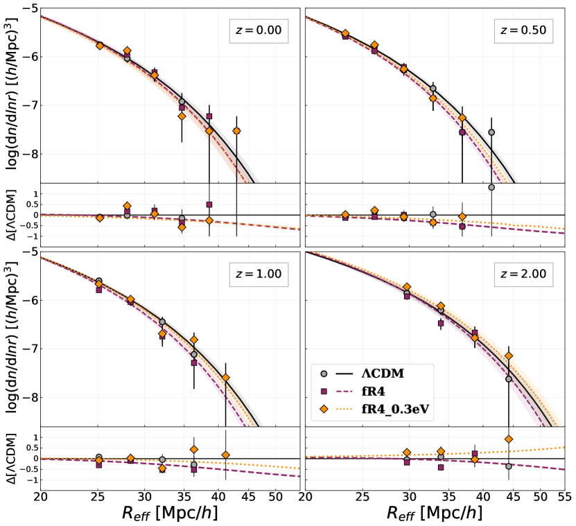
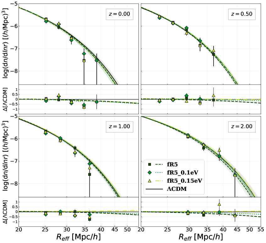
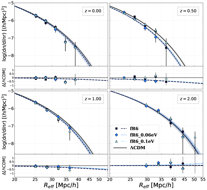
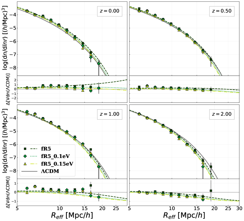
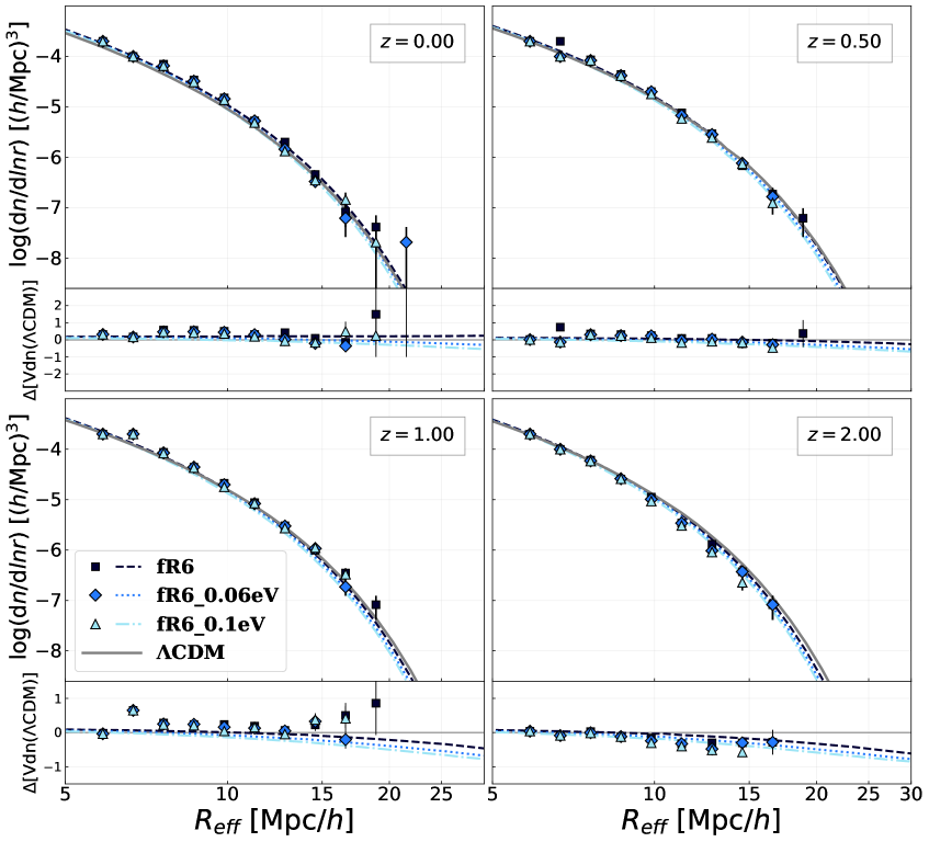
In Fig. 9 we report the comparison between the measured void abundance for the $\Lambda$CDM, fR4 and fR4_0.3eV models, showing also the corresponding predictions of the Vdn model computed for each cosmological scenario. The shaded region around each curve represents the uncertainty derived from the propagation of the error associated to the value of $b_{\mathrm{eff}}$ computed for each case, converted by means of Eq. (27), and used to compute the theoretical models. The residuals reported in the bottom sub-panels are computed as the difference from the theoretical void size function of the $\Lambda$CDM model, in units of the latter, for both the measured and the predicted abundances. We find a good agreement between the predictions of the reparametrised Vdn model and the measured void size functions. Nevertheless, the cosmic voids found in the DM halo simulations are so rare that the Poissonian noise does not allow us to distinguish a specific trend for the abundances measured in MG and massive neutrinos scenarios. This was previously verified also in other works analysing voids identified in biased tracers using cosmological simulations in MG gravity scenarios or with massive neutrinos (Voivodic et al., 2017; Kreisch et al., 2019). In Fig. 10 we show the results for the remaining cosmological models. Even more in these cases, the void abundances derived in different cosmologies are hardly discernable from the $\Lambda$CDM ones. The signal is stronger at higher redshifts due to the fact that the underdensity threshold used to rescale the voids moves towards values closer to $0$ for higher values of $b_{\mathrm{eff}}$ (see Eq. (21)). This causes the growth of the population of large voids and can lead to an overall increase of the number of voids with radii belonging to the range considered in this analysis. However, since this method implies the selection of shallower voids, it will be important to verify the purity of the void sample when it derives from real galaxy surveys, and thus to take into account the possible contamination by Poissonian noise. The accuracy of the measured void counts at high redshifts can be in fact compromised by systematic uncertainties still not parameterised in the model. Nevertheless, in our case the prescriptions adopted to prepare the void samples are proven to be compliant with the theoretical predictions and do not require further procedures of removal of spurious voids.

Given the poor statistics of the measured void counts and thus the large uncertainties associated to the data, we focus now on the analysis of the predicted abundances only. We first point out that, although from these plots the void counts could appear reduced in MG cosmologies, this is true in fact only for the large sizes. Looking at the Figures 9 and 10, we note that the void size functions in the different cosmological models considered are significantly different only for large radii, an effect that is larger for higher values of the $f_{R0}$ parameter. While at $z=0$ the predictions of the Vdn model for MG cosmologies with and without massive neutrinos are statistically indistinguishable, at intermediate redshifts the presence of massive neutrinos causes a shift of the void size function towards the one obtained for the standard $\Lambda$CDM model. This trend results even more relevant at $z=2$, where the effect of the neutrino thermal free-streaming brings the theoretical curve above the one of the $\Lambda$CDM case. This outcome might seem counterintuitive, since the presence of massive neutrinos leads effectively to a slow down of the evolution cosmic voids. Nevertheless, this trend has been identified also in Kreisch et al. (2019) using a methodology similar to the one reported in this paper to select and characterise the void sample. This phenomenon is in fact due to the effect of the adopted bias-dependent threshold, that causes a rescaling of the detected underdensities toward greater radii and appears more evident for larger voids. This is an obvious indicator of the possibility to use cosmic void abundances to disentangle the degeneracies between MG and massive neutrinos models. However, we recall that the effect of the tracer bias on the void size function may be partially compensated by the one of massive neutrinos and MG models, therefore the trends found in this analysis may be different using other simulations or different tracers (see also Kreisch et al., 2019).

Table 2: The most relevant quantities related to the voids identified in the distribution of 200c haloes. The table is structured in $4$ parts, which separate the values computed for different redshifts. Each line shows the set of data relative to each of the cosmological models analysed in this work. The values of the tracer effective bias used to reparametrise the Vdn model are reported in the column named $b_{\mathrm{eff}}$. The following column provides the void abundances predicted by the theory, obtained by integrating the Vdn model over the range of void radii described in this section. Then we report the number of voids extracted from the void catalogues built with VIDE, for completeness. The last columns represent the void counts derived from the catalogues of voids, modelled with the cleaning algorithm, measured on the same range of void radii used to compute the theoretical abundances.

Cosmological model	$b_{\mathrm{eff}}$	Vdn model	VIDE voids	Cleaned voids	$b_{\mathrm{eff}}$	Vdn model	VIDE voids	Cleaned voids
	$z=0$				$z=0.5$
$\Lambda$CDM	$1.147\pm 0.009$	$119\pm 16$	$703\pm 27$	$109\pm 10$	$1.44\pm 0.01$	$193\pm 17$	$949\pm 31$	$185\pm 14$
fR4	$1.036\pm 0.008$	$111\pm 19$	$682\pm 26$	$117\pm 11$	$1.30\pm 0.01$	$163\pm 18$	$912\pm 30$	$168\pm 13$
fR4_0.3eV	$1.099\pm 0.009$	$104\pm 16$	$703\pm 27$	$119\pm 11$	$1.42\pm 0.01$	$173\pm 17$	$941\pm 31$	$199\pm 14$
fR5	$1.103\pm 0.009$	$116\pm 17$	$690\pm 26$	$112\pm 11$	$1.40\pm 0.01$	$192\pm 17$	$919\pm 30$	$179\pm 13$
fR5_0.1eV	$1.124\pm 0.009$	$112\pm 16$	$679\pm 26$	$107\pm 10$	$1.44\pm 0.01$	$199\pm 17$	$930\pm 30$	$170\pm 13$
fR5_0.15eV	$1.140\pm 0.009$	$113\pm 16$	$683\pm 26$	$126\pm 11$	$1.47\pm 0.01$	$201\pm 17$	$922\pm 30$	$177\pm 13$
fR6	$1.116\pm 0.008$	$108\pm 16$	$702\pm 26$	$96\pm 8$	$1.35\pm 0.01$	$149\pm 15$	$907\pm 30$	$180\pm 13$
fR6_0.06eV	$1.131\pm 0.009$	$107\pm 15$	$715\pm 27$	$113\pm 11$	$1.37\pm 0.01$	$148\pm 15$	$900\pm 30$	$165\pm 13$
fR6_0.1eV	$1.140\pm 0.009$	$106\pm 15$	$723\pm 27$	$113\pm 11$	$1.39\pm 0.01$	$153\pm 15$	$929\pm 30$	$173\pm 13$
	$z=1$				$z=2$
$\Lambda$CDM	$1.90\pm 0.01$	$154\pm 17$	$734\pm 27$	$152\pm 12$	$3.18\pm 0.03$	$97\pm 17$	$470\pm 22$	$92\pm 10$
fR4	$1.73\pm 0.01$	$129\pm 13$	$727\pm 27$	$108\pm 10$	$3.05\pm 0.03$	$92\pm 15$	$435\pm 21$	$73\pm 9$
fR4_0.3eV	$1.92\pm 0.02$	$147\pm 15$	$731\pm 27$	$140\pm 12$	$3.44\pm 0.04$	$114\pm 18$	$469\pm 22$	$121\pm 11$
fR5	$1.85\pm 0.01$	$154\pm 16$	$750\pm 27$	$133\pm 12$	$3.03\pm 0.03$	$85\pm 14$	$460\pm 21$	$73\pm 9$
fR5_0.1eV	$1.90\pm 0.01$	$155\pm 16$	$743\pm 27$	$120\pm 11$	$3.16\pm 0.03$	$93\pm 16$	$477\pm 22$	$90\pm 9$
fR5_0.15eV	$1.95\pm 0.02$	$164\pm 17$	$742\pm 27$	$125\pm 11$	$3.26\pm 0.04$	$101\pm 17$	$479\pm 22$	$93\pm 10$
fR6	$1.82\pm 0.01$	$132\pm 15$	$744\pm 27$	$125\pm 11$	$3.16\pm 0.03$	$98\pm 17$	$456\pm 21$	$96\pm 10$
fR6_0.06eV	$1.85\pm 0.01$	$136\pm 16$	$737\pm 27$	$136\pm 12$	$3.24\pm 0.04$	$103\pm 17$	$484\pm 22$	$101\pm 10$
fR6_0.1eV	$1.87\pm 0.01$	$136\pm 16$	$742\pm 27$	$128\pm 11$	$3.27\pm 0.04$	$103\pm 17$	$468\pm 22$	$111\pm 11$

To facilitate the comparison of these results and maximise the signal obtained from the measured void abundance, we compare now the total void number counts with the abundance computed by integrating the theoretical void size function over the same range of radiiEven if the total void counts is not commonly used to derive cosmological constraints, it can constitute in this case a useful quantity to analyse. Indeed, it allows to perform a simple validation of the predictions of the void size function models, collapsing the information on void number counts related to different spatial scales and sharping the signal achieved from the measured abundances. We present in Table 2 the comparison between the integrated values of void number counts obtained from the theoretical models and our measurements, for each of the cosmological models and redshifts explored in this work. We report also the value of the tracer effective bias, used to reparametrise the characteristic threshold of the Vdn model. Then we show, for completeness, the measured abundance derived from the VIDE void catalogues before performing the cleaning procedure. The abundances extracted from the raw VIDE void catalogues are significantly larger than those obtained after the cleaning procedure, but they are clearly not in agreement with the Vdn model predictions. This outcome is not surprising since these voids are not modelled according to the excursion-set theory described in Section 2.3. Now we focus on the comparison of the total counts of cleaned voids with the predictions achieved with the reparametrised Vdn model. The errors associated with the latter are evaluated by propagating the uncertainties related to $b_{\mathrm{eff}}$ and $b_{\mathrm{punct}}$ during the calibration of the function $\mathcal{F}(b_{\mathrm{eff}})$, while those associated with the measured void abundances are assumed to be Poissonian. We can see that the theoretical void abundances are overall consistent with the observed ones, considering the uncertainties on both the values. As expected from the results shown in Figures 9 and 10, a significant differentiation between the analysed cosmological models is reached at $z=2$, despite the scarcity of void counts makes their distinction challenging. Indeed, the simulations considered in this work do not allow us to have enough statistics for large voids at high redshifts.

5 CONCLUSIONS

In this work we have investigated the possibility of disentangling the degeneracies characterising cosmological models that simultaneously feature a modification of GR – in the form of $f(R)$ gravity – and the presence of massive neutrinos. To explore possible observational differences among these scenarios, we have focused on the exploitation of cosmic void density profiles and abundances. We have built void catalogues by means of the void detection algorithm VIDE, identifying voids in both the DM particle and halo distributions, for all the different cosmological models at our disposal, at the redshifts $z=0,0.5,1,2$. For the analysis of the void size function, we adopted the procedure described in Contarini et al. (2019), modelling cosmic voids according to the theoretical definition provided by the Vdn model.

The main results obtained in this work can be summarised as follows:

• The analysis of the void stacked density profiles, measured in both the DM and halo distributions, has revealed some deviations of the MG model profiles from those computed in a $\Lambda$CDM cosmology, more evident for the most extreme scenarios. These differences are particularly strong at $z=1$, when the growth of cosmic structures shows an enhancement given by the effect of the fifth force. Nevertheless, the neutrino thermal free-streaming almost completely erases any peculiar trend of the density profiles, making void profiles measured for these models almost indistinguishable compared to the $\Lambda$CDM ones.

• We have found an excellent agreement between the measured abundances and the theoretical predictions obtained with the Vdn model for voids identified in the DM particle distribution in different cosmological models. Furthermore, while at low redshifts the presence of massive neutrinos tends to lower the void size function computed for MG models towards the one relative to the $\Lambda$CDM scenario, at high redshifts this effect results in an excessive reduction in the void abundance. This inversion of the trend is caused by the different redshift dependence of MG and massive neutrinos imprints on structure formation. In fact, the effect of massive neutrinos to damp the evolution of voids is already in place at early epochs when MG effects are still negligible.

• We have fitted a linear function $\mathcal{F}$ to model the relation between the tracer bias computed on large scales, $b_{\mathrm{eff}}$, and the one measured inside cosmic voids, $b_{\mathrm{punct}}$. We have considered two selection criteria to build samples of viralised DM haloes with different compactness, characterised by an internal density equal to $200$ and $500$ times the critical density of the Universe, respectively. From the comparison between the coefficients of the function $\mathcal{F}$ obtained using these different types of biased tracers, we have identified the presence of a trend characterising the relation between $b_{\mathrm{eff}}$ and $b_{\mathrm{punct}}$. This appears as a slight dependence on the type of objects used to identify voids, related in particular to the criterion applied to define the mass tracers. We have also tested the universality of the calibrated relation for a specific selection of mass tracers. In particular, using 200c haloes, we have compared the linear function obtained for $\Lambda$CDM model with those computed using non-standard cosmological models, verifying that the calibrations performed for the different scenarios are statistically consistent.

• With the parametrisation of the threshold of the Vdn model by means of the function $\mathcal{F}(b_{\mathrm{eff}})$, we have compared the measured and predicted abundances of voids identified in the 200c halo catalogues. We have found a good agreement between the void size functions measured in the simulated void catalogues and the predicted ones, in the full range of void radii probed by our simulations. For these sizes, all the cosmological models considered in this work predict statistically indistinguishable void abundances. Larger simulations are required to push the analysis at larger voids, where the differences in the size function of cosmic voids are expected to be larger, thus allowing to break the cosmic degeneracies.

We can conclude that the void density profiles do not allow to disentangle the cosmic degeneracies given by the proper combination of the $f_{R0}$ and $m_{v}$ parameters. On the other hand, void abundances have been shown to be a promising probe to break these degeneracies, though larger simulation volumes are needed to extract more precise and accurate results for bigger voids at higher redshifts. The requirement for a proper exploitation of this probe is therefore the exploration of wide and deep regions of the Universe, with the goal of obtaining a statistically relevant number of voids with large radii, at $z>1$. Future spectroscopic surveys like WFIRST, Euclid and LSST, will serve to this purpose, allowing to achieve the cosmic void statistics required to disentangle the degenerate effects of MG and massive neutrino scenarios.

Data Availability

The simulation data underlying this article will be shared on reasonable request to the corresponding author.

References

- Abel et al. (2012) Abel T., Hahn O., Kaehler R., 2012, MNRAS, 427, 61
- Agarwal & Feldman (2011) Agarwal S., Feldman H. A., 2011, MNRAS, 410, 1647
- Ahmed et al. (2004) Ahmed S. N., et al., 2004, Phys. Rev. Lett., 92, 181301
- Amendola et al. (2018) Amendola L., et al., 2018, Living Reviews in Relativity, 21, 2
- Aubert et al. (2020) Aubert M., et al., 2020, arXiv e-prints, p. arXiv:2007.09013
- Baker et al. (2018) Baker T., Clampitt J., Jain B., Trodden M., 2018, Phys. Rev. D, 98, 023511
- Baldi (2012) Baldi M., 2012, MNRAS, 422, 1028
- Baldi et al. (2014) Baldi M., Villaescusa-Navarro F., Viel M., Puchwein E., Springel V., Moscardini L., 2014, MNRAS, 440, 75
- Banerjee & Dalal (2016) Banerjee A., Dalal N., 2016, J. Cosmology Astropart. Phys., 2016, 015
- Barreira et al. (2015) Barreira A., Cautun M., Li B., Baugh C. M., Pascoli S., 2015, J. Cosmology Astropart. Phys., 2015, 028
- Becker-Szendy et al. (1992) Becker-Szendy R., et al., 1992, Phys. Rev. D, 46, 3720
- Bennett et al. (2013) Bennett C. L., et al., 2013, ApJS, 208, 20
- Bernal et al. (2016) Bernal J. L., Verde L., Riess A. G., 2016, J. Cosmology Astropart. Phys., 2016, 019
- Bernardeau (1994) Bernardeau F., 1994, ApJ, 427, 51
- Bertotti et al. (2003) Bertotti B., Iess L., Tortora P., 2003, Nature, 425, 374
- Bianchi & Rovelli (2010) Bianchi E., Rovelli C., 2010, arXiv e-prints, p. arXiv:1002.3966
- Blumenthal et al. (1992) Blumenthal G. R., da Costa L. N., Goldwirth D. S., Lecar M., Piran T., 1992, ApJ, 388, 234
- Bond et al. (1991) Bond J. R., Cole S., Efstathiou G., Kaiser N., 1991, ApJ, 379, 440
- Brandbyge & Hannestad (2009) Brandbyge J., Hannestad S., 2009, J. Cosmology Astropart. Phys., 2009, 002
- Brandbyge & Hannestad (2010) Brandbyge J., Hannestad S., 2010, J. Cosmology Astropart. Phys., 2010, 021
- Brandbyge et al. (2008) Brandbyge J., Hannestad S., Haugbølle T., Thomsen B., 2008, J. Cosmology Astropart. Phys., 2008, 020
- Brandbyge et al. (2010) Brandbyge J., Hannestad S., Haugbølle T., Wong Y. Y. Y., 2010, J. Cosmology Astropart. Phys., 2010, 014
- Brax & Valageas (2013) Brax P., Valageas P., 2013, Phys. Rev. D, 88, 023527
- Brax & Valageas (2014) Brax P., Valageas P., 2014, Phys. Rev. D, 90, 023507
- Cai et al. (2014) Cai Y.-C., Padilla N., Li B., 2014, arXiv e-prints, p. arXiv:1410.8355
- Carroll (2001) Carroll S. M., 2001, Living Reviews in Relativity, 4, 1
- Castorina et al. (2014) Castorina E., Sefusatti E., Sheth R. K., Villaescusa-Navarro F., Viel M., 2014, J. Cosmology Astropart. Phys., 2014, 049
- Castorina et al. (2015) Castorina E., Carbone C., Bel J., Sefusatti E., Dolag K., 2015, J. Cosmology Astropart. Phys., 2015, 043
- Cataneo et al. (2015) Cataneo M., et al., 2015, Phys. Rev. D, 92, 044009
- Chan et al. (2019) Chan H. Y. J., Chiba M., Ishiyama T., 2019, MNRAS, 490, 2405
- Chiang et al. (2019) Chiang C.-T., LoVerde M., Villaescusa-Navarro F., 2019, Phys. Rev. Lett., 122, 041302
- Clampitt et al. (2013) Clampitt J., Cai Y.-C., Li B., 2013, MNRAS, 431, 749
- Clifton et al. (2012) Clifton T., Ferreira P. G., Padilla A., Skordis C., 2012, Phys. Rep., 513, 1
- Cole (1991) Cole S., 1991, ApJ, 367, 45
- Contarini et al. (2019) Contarini S., Ronconi T., Marulli F., Moscardini L., Veropalumbo A., Baldi M., 2019, MNRAS, 488, 3526
- Correa et al. (2020) Correa C. M., Paz D. J., Sánchez A. G., Ruiz A. N., Padilla N. D., Angulo R. E., 2020, arXiv e-prints, p. arXiv:2007.12064
- Cousinou et al. (2019) Cousinou M. C., Pisani A., Tilquin A., Hamaus N., Hawken A. J., Escoffier S., 2019, Astronomy and Computing, 27, 53
- Cuesta et al. (2016) Cuesta A. J., Niro V., Verde L., 2016, Physics of the Dark Universe, 13, 77
- Despali et al. (2016) Despali G., Giocoli C., Angulo R. E., Tormen G., Sheth R. K., Baso G., Moscardini L., 2016, MNRAS, 456, 2486
- Dolgov & Kawasaki (2003) Dolgov A. D., Kawasaki M., 2003, Physics Letters B, 573, 1
- Dvorkin et al. (2019) Dvorkin C., et al., 2019, BAAS, 51, 64
- Eisenstein et al. (2005) Eisenstein D. J., et al., 2005, ApJ, 633, 560
- Falck et al. (2018) Falck B., Koyama K., Zhao G.-B., Cautun M., 2018, MNRAS, 475, 3262
- Frieman et al. (2008) Frieman J. A., Turner M. S., Huterer D., 2008, ARA&A, 46, 385
- Fukuda et al. (1998) Fukuda Y., et al., 1998, Phys. Rev. Lett., 81, 1562
- Furlanetto & Piran (2006) Furlanetto S. R., Piran T., 2006, MNRAS, 366, 467
- García-Farieta et al. (2019) García-Farieta J. E., Marulli F., Veropalumbo A., Moscardini L., Casas-Mirand a R. A., Giocoli C., Baldi M., 2019, MNRAS, 488, 1987
- Giocoli et al. (2008) Giocoli C., Tormen G., van den Bosch F. C., 2008, MNRAS, 386, 2135
- Giocoli et al. (2018) Giocoli C., Baldi M., Moscardini L., 2018, MNRAS, 481, 2813
- Green et al. (2012) Green J., et al., 2012, arXiv e-prints, p. arXiv:1208.4012
- Hagstotz et al. (2019a) Hagstotz S., Costanzi M., Baldi M., Weller J., 2019a, MNRAS, 486, 3927
- Hagstotz et al. (2019b) Hagstotz S., Gronke M., Mota D., Baldi M., 2019b, Astron. Astrophys., 629, A46
- Hahn et al. (2015) Hahn O., Angulo R. E., Abel T., 2015, MNRAS, 454, 3920
- Hamaus et al. (2014) Hamaus N., Sutter P. M., Wandelt B. D., 2014, Physical Review Letters, 112, 251302
- Hamaus et al. (2016) Hamaus N., Pisani A., Sutter P. M., Lavaux G., Escoffier S., Wand elt B. D., Weller J., 2016, Phys. Rev. Lett., 117, 091302
- Hamaus et al. (2017) Hamaus N., Cousinou M.-C., Pisani A., Aubert M., Escoffier S., Weller J., 2017, J. Cosmology Astropart. Phys., 2017, 014
- Hamaus et al. (2020) Hamaus N., Pisani A., Choi J.-A., Lavaux G., Wandelt B. D., Weller J., 2020, arXiv e-prints, p. arXiv:2007.07895
- Hawken et al. (2020) Hawken A. J., Aubert M., Pisani A., Cousinou M.-C., Escoffier S., Nadathur S., Rossi G., Schneider D. P., 2020, J. Cosmology Astropart. Phys., 2020, 012
- He (2013) He J.-h., 2013, Phys. Rev. D, 88, 103523
- Heavens et al. (2017) Heavens A., Fantaye Y., Sellentin E., Eggers H., Hosenie Z., Kroon S., Mootoovaloo A., 2017, Phys. Rev. Lett., 119, 101301
- Hinterbichler & Khoury (2010) Hinterbichler K., Khoury J., 2010, Phys. Rev. Lett., 104, 231301
- Hojjati et al. (2011) Hojjati A., Pogosian L., Zhao G.-B., 2011, J. Cosmology Astropart. Phys., 2011, 005
- Hu & Sawicki (2007) Hu W., Sawicki I., 2007, Phys. Rev. D, 76, 064004
- Ishak (2019) Ishak M., 2019, Living Reviews in Relativity, 22, 1
- Jennings et al. (2013) Jennings E., Li Y., Hu W., 2013, MNRAS, 434, 2167
- Joyce et al. (2015) Joyce A., Jain B., Khoury J., Trodden M., 2015, Phys. Rep., 568, 1
- Khoury & Weltman (2004) Khoury J., Weltman A., 2004, Phys. Rev. Lett., 93, 171104
- Komatsu et al. (2011) Komatsu E., et al., 2011, ApJS, 192, 18
- Kreisch et al. (2019) Kreisch C. D., Pisani A., Carbone C., Liu J., Hawken A. J., Massara E., Spergel D. N., Wandelt B. D., 2019, MNRAS, 488, 4413
- Kumar & Nunes (2016) Kumar S., Nunes R. C., 2016, Phys. Rev. D, 94, 123511
- LSST Dark Energy Science Collaboration (2012) LSST Dark Energy Science Collaboration 2012, arXiv e-prints, p. arXiv:1211.0310
- Laureijs et al. (2011) Laureijs R., et al., 2011, arXiv e-prints, p. arXiv:1110.3193
- Lazeyras et al. (2020) Lazeyras T., Villaescusa-Navarro F., Viel M., 2020, arXiv e-prints, p. arXiv:2008.12265
- Le Verrier (1859) Le Verrier U. J., 1859, Annales de l’Observatoire de Paris, 5, 1
- Lesgourgues et al. (2013) Lesgourgues J., Mangano G., Miele G., Pastor S., 2013, Neutrino Cosmology
- Lewis et al. (2000) Lewis A., Challinor A., Lasenby A., 2000, ApJ, 538, 473
- Lu et al. (2015) Lu J.-S., Cao J., Li Y.-F., Zhou S., 2015, J. Cosmology Astropart. Phys., 2015, 044
- Lu et al. (2016) Lu J., Liu M., Wu Y., Wang Y., Yang W., 2016, European Physical Journal C, 76, 679
- Mangano et al. (2005) Mangano G., Miele G., Pastor S., Pinto T., Pisanti O., Serpico P. D., 2005, Nuclear Physics B, 729, 221
- Martin (2012) Martin J., 2012, Comptes Rendus Physique, 13, 566
- Martino & Sheth (2009) Martino M. C., Sheth R. K., 2009, arXiv e-prints, p. arXiv:0911.1829
- Marulli et al. (2011) Marulli F., Carbone C., Viel M., Moscardini L., Cimatti A., 2011, MNRAS, 418, 346
- Marulli et al. (2013) Marulli F., et al., 2013, A&A, 557, A17
- Marulli et al. (2016) Marulli F., Veropalumbo A., Moresco M., 2016, Astronomy and Computing, 14, 35
- Marulli et al. (2018) Marulli F., et al., 2018, A&A, 620, A1
- Massara & Sheth (2018) Massara E., Sheth R. K., 2018, arXiv e-prints, p. arXiv:1811.03132
- Massara et al. (2015) Massara E., Villaescusa-Navarro F., Viel M., Sutter P. M., 2015, J. Cosmology Astropart. Phys., 2015, 018
- Merten et al. (2019) Merten J., Giocoli C., Baldi M., Meneghetti M., Peel A., Lalande F., Starck J.-L., Pettorino V., 2019, MNRAS, 487, 104
- Mo & White (1996) Mo H. J., White S. D. M., 1996, MNRAS, 282, 347
- Moresco & Marulli (2017) Moresco M., Marulli F., 2017, MNRAS, 471, L82
- Motohashi et al. (2013) Motohashi H., Starobinsky A. A., Yokoyama J., 2013, Phys. Rev. Lett., 110, 121302
- Nadathur & Hotchkiss (2015a) Nadathur S., Hotchkiss S., 2015a, MNRAS, 454, 2228
- Nadathur & Hotchkiss (2015b) Nadathur S., Hotchkiss S., 2015b, MNRAS, 454, 889
- Nadathur et al. (2016) Nadathur S., Hotchkiss S., Diego J. M., Iliev I. T., Gottlöber S., Watson W. A., Yepes G., 2016, in van de Weygaert R., Shandarin S., Saar E., Einasto J., eds, IAU Symposium Vol. 308, The Zeldovich Universe: Genesis and Growth of the Cosmic Web. pp 542–545 (arXiv:1412.8372), doi:10.1017/S1743921316010541
- Nadathur et al. (2020) Nadathur S., et al., 2020, arXiv e-prints, p. arXiv:2008.06060
- Neyrinck (2008) Neyrinck M. C., 2008, MNRAS, 386, 2101
- Nojiri & Odintsov (2006) Nojiri S., Odintsov S. D., 2006, arXiv e-prints, pp hep–th/0601213
- Padilla et al. (2016) Padilla N. D., Paz D., Lares M., Ceccarelli L., Lambas D. G. A., Cai Y.-C., Li B., 2016, in van de Weygaert R., Shandarin S., Saar E., Einasto J., eds, IAU Symposium Vol. 308, The Zeldovich Universe: Genesis and Growth of the Cosmic Web. pp 530–537, doi:10.1017/S1743921316010528
- Paz et al. (2013) Paz D., Lares M., Ceccarelli L., Padilla N., Lambas D. G., 2013, MNRAS, 436, 3480
- Peel et al. (2018) Peel A., Pettorino V., Giocoli C., Starck J.-L., Baldi M., 2018, A&A, 619, A38
- Peel et al. (2019) Peel A., Lalande F., Starck J.-L., Pettorino V., Merten J., Giocoli C., Meneghetti M., Baldi M., 2019, Phys. Rev. D, 100, 023508
- Perico et al. (2019) Perico E. L. D., Voivodic R., Lima M., Mota D. F., 2019, A&A, 632, A52
- Perlmutter et al. (1999) Perlmutter S., et al., 1999, ApJ, 517, 565
- Pisani et al. (2014) Pisani A., Lavaux G., Sutter P. M., Wandelt B. D., 2014, MNRAS, 443, 3238
- Pisani et al. (2015) Pisani A., Sutter P. M., Hamaus N., Alizadeh E., Biswas R., Wandelt B. D., Hirata C. M., 2015, Phys. Rev. D, 92, 083531
- Pisani et al. (2019) Pisani A., et al., 2019, BAAS, 51, 40
- Planck Collaboration et al. (2016) Planck Collaboration et al., 2016, A&A, 594, A13
- Planck Collaboration et al. (2018) Planck Collaboration et al., 2018, arXiv e-prints, p. arXiv:1807.06209
- Pollina et al. (2016) Pollina G., Baldi M., Marulli F., Moscardini L., 2016, MNRAS, 455, 3075
- Pollina et al. (2017) Pollina G., Hamaus N., Dolag K., Weller J., Baldi M., Moscardini L., 2017, MNRAS, 469, 787
- Pollina et al. (2019) Pollina G., et al., 2019, MNRAS, 487, 2836
- Poulin et al. (2018) Poulin V., Boddy K. K., Bird S., Kamionkowski M., 2018, Phys. Rev. D, 97, 123504
- Press & Schechter (1974) Press W. H., Schechter P., 1974, ApJ, 193, 437
- Puchwein et al. (2013) Puchwein E., Baldi M., Springel V., 2013, MNRAS, 436, 348
- Ricciardelli et al. (2014) Ricciardelli E., Quilis V., Varela J., 2014, MNRAS, 440, 601
- Riemer-Sørensen et al. (2013) Riemer-Sørensen S., Parkinson D., Davis T. M., Blake C., 2013, ApJ, 763, 89
- Riess et al. (1998) Riess A. G., et al., 1998, AJ, 116, 1009
- Ronconi & Marulli (2017) Ronconi T., Marulli F., 2017, A&A, 607, A24
- Ronconi et al. (2019) Ronconi T., Contarini S., Marulli F., Baldi M., Moscardini L., 2019, arXiv e-prints: 1902.04585,
- Sahlén (2019) Sahlén M., 2019, Phys. Rev. D, 99, 063525
- Sahlén & Silk (2018) Sahlén M., Silk J., 2018, Phys. Rev. D, 97, 103504
- Sahlén et al. (2016) Sahlén M., Zubeldía Í., Silk J., 2016, ApJ, 820, L7
- Saito et al. (2008) Saito S., Takada M., Taruya A., 2008, Phys. Rev. Lett., 100, 191301
- Saito et al. (2009) Saito S., Takada M., Taruya A., 2009, Phys. Rev. D, 80, 083528
- Schmidt et al. (1998) Schmidt B. P., et al., 1998, ApJ, 507, 46
- Schuster et al. (2019) Schuster N., Hamaus N., Pisani A., Carbone C., Kreisch C. D., Pollina G., Weller J., 2019, J. Cosmology Astropart. Phys., 2019, 055
- Seljak et al. (2006) Seljak U., Slosar A., McDonald P., 2006, J. Cosmology Astropart. Phys., 2006, 014
- Shafieloo & Clarkson (2010) Shafieloo A., Clarkson C., 2010, Phys. Rev. D, 81, 083537
- Shandarin (2011) Shandarin S. F., 2011, J. Cosmology Astropart. Phys., 2011, 015
- Sheth & Tormen (1999) Sheth R. K., Tormen G., 1999, MNRAS, 308, 119
- Sheth & van de Weygaert (2004) Sheth R. K., van de Weygaert R., 2004, MNRAS, 350, 517
- Sheth et al. (2001) Sheth R. K., Mo H. J., Tormen G., 2001, MNRAS, 323, 1
- Spolyar et al. (2013) Spolyar D., Sahlén M., Silk J., 2013, Phys. Rev. Lett., 111, 241103
- Springel (2005) Springel V., 2005, MNRAS, 364, 1105
- Sutter et al. (2014a) Sutter P. M., Lavaux G., Hamaus N., Wand elt B. D., Weinberg D. H., Warren M. S., 2014a, MNRAS, 442, 462
- Sutter et al. (2014b) Sutter P. M., Elahi P., Falck B., Onions J., Hamaus N., Knebe A., Srisawat C., Schneider A., 2014b, MNRAS, 445, 1235
- Sutter et al. (2015) Sutter P. M., et al., 2015, Astronomy and Computing, 9, 1
- Tinker et al. (2010) Tinker J. L., Robertson B. E., Kravtsov A. V., Klypin A., Warren M. S., Yepes G., Gottlöber S., 2010, ApJ, 724, 878
- Tormen et al. (2004) Tormen G., Moscardini L., Yoshida N., 2004, MNRAS, 350, 1397
- Verde et al. (2019) Verde L., Treu T., Riess A. G., 2019, Nature Astronomy, 3, 891
- Verza et al. (2019) Verza G., Pisani A., Carbone C., Hamaus N., Guzzo L., 2019, J. Cosmology Astropart. Phys., 2019, 040
- Viel et al. (2010) Viel M., Haehnelt M. G., Springel V., 2010, J. Cosmology Astropart. Phys., 2010, 015
- Villaescusa-Navarro et al. (2013a) Villaescusa-Navarro F., Vogelsberger M., Viel M., Loeb A., 2013a, MNRAS, 431, 3670
- Villaescusa-Navarro et al. (2013b) Villaescusa-Navarro F., Bird S., Peña-Garay C., Viel M., 2013b, J. Cosmology Astropart. Phys., 2013, 019
- Villaescusa-Navarro et al. (2014) Villaescusa-Navarro F., Marulli F., Viel M., Branchini E., Castorina E., Sefusatti E., Saito S., 2014, J. Cosmology Astropart. Phys., 2014, 011
- Voivodic et al. (2017) Voivodic R., Lima M., Llinares C., Mota D. F., 2017, Phys. Rev. D, 95, 024018
- Wagner et al. (2012) Wagner C., Verde L., Jimenez R., 2012, ApJ, 752, L31
- Wang et al. (2019) Wang Y., et al., 2019, BAAS, 51, 508
- Weinberg (1989) Weinberg S., 1989, Reviews of Modern Physics, 61, 1
- Wen et al. (2018) Wen S., Wang S., Luo X., 2018, J. Cosmology Astropart. Phys., 2018, 011
- Will (2005) Will C. M., 2005, Phys. Rev. D, 71, 084027
- Wright et al. (2017) Wright B. S., Winther H. A., Koyama K., 2017, J. Cosmology Astropart. Phys., 2017, 054
- Yèche et al. (2017) Yèche C., Palanque-Delabrouille N., Baur J., du Mas des Bourboux H., 2017, J. Cosmology Astropart. Phys., 2017, 047
- Yoo & Watanabe (2012) Yoo J., Watanabe Y., 2012, International Journal of Modern Physics D, 21, 1230002
- Zeng & White (1991) Zeng N., White S. D. M., 1991, ApJ, 374, 1
- Zennaro et al. (2018) Zennaro M., Bel J., Dossett J., Carbone C., Guzzo L., 2018, MNRAS, 477, 491
- Zhao et al. (2009) Zhao G.-B., Pogosian L., Silvestri A., Zylberberg J., 2009, Phys. Rev. D, 79, 083513
- Zucca et al. (2019) Zucca A., Pogosian L., Silvestri A., Zhao G. B., 2019, J. Cosmology Astropart. Phys., 2019, 001