Morley Finite Element Method for the
von Kármán Obstacle Problem

Abstract

This paper focusses on the von Kármán equations  for the moderately large deformation of a very thin plate with the convex obstacle constraint leading to a coupled system of semilinear fourth-order obstacle problem and motivates its nonconforming Morley finite element approximation. The first part establishes the well-posedness of the von Kármán  obstacle problem and also discusses the uniqueness of the solution under an a priori and an a posteriori smallness condition on the data. The second part of the article discusses the regularity result of Frehse from 1971 and combines it with the regularity of the solution on a polygonal domain. The third part of the article shows an a priori error estimate for optimal convergence rates for the Morley finite element approximation to the von Kármán obstacle problem for small data. The article concludes with numerical results that illustrates the requirement of smallness assumption on the data for optimal convergence rate.

1 Introduction

Short history of related work. The von Kármán equations [17] model the bending of very thin elastic plates through a system of fourth-order semi-linear elliptic equations; cf. [2, 17, 23] and references therein for the existence of solutions, regularity, and bifurcation phenomena. The papers [9, 27, 31, 32, 25, 5, 12, 13] study the approximation and error bounds for regular solutions to von Kármán equations  using conforming, mixed, hybrid, Morley, $C^{0}$ interior penalty and discontinuous Galerkin finite element methods (FEMs).

The obstacle problem is a prototypical example for a variational inequality and arises in contact mechanics, option pricing, and fluid flow problems. The location of the free boundary is not known a priori and forms a part of the solution procedure. For the theoretical and numerical aspects of variational inequalities, see [20, 22]. A unified convergence analysis for the fourth-order linear two-sided obstacle problem of clamped Kirchhoff plates in [8, 7, 6] studies $C^{1}$ FEMs, $C^{0}$ interior penalty methods, and classical nonconforming FEMs on convex domains and, analyse the $C^{0}$ interior penalty and the Morley FEM on polygonal domains.

The obstacle problem for von Kármán equations  with a nonlinearity together with a free boundary offers additional difficulties. The obstacle problem in [28, 33, 26] concerns a different plate model with continuation, spectral, and complementarity methods, while the papers [29, 30] study conforming penalty FEM.

The present paper is the first on the fourth-order semilinear obstacle problem of a (very thin) von Kármán  plate. The article derives existence, uniqueness (under smallness assumption on data) and regularity results of the von Kármán  obstacle problem. Nonconforming FEMs appear to be more attractive than the classical $C^{1}$ conforming FEMs, so this article suggests the Morley FEM to approximate the von Kármán  obstacle problem and derives an optimal order a priori error estimate with the best approximation plus a linear perturbation.

Problem Formulation. Given an obstacle $\chi\in H^{2}(\Omega)$ with $\max\chi(\partial\Omega):=\max_{x\in\partial\Omega}\chi(x)<0$, define the non-empty, closed, and convex subset

$$K:=\{\varphi\in H^{2}_{0}(\Omega):\varphi\geq\chi\mbox{ a.e. in }\Omega\}$$

of $H^{2}_{0}(\Omega)$ in a bounded polygonal domain $\Omega\subset\mathbb{R}^{2}.$ The Hessian $D^{2}$ and von Kármán  bracket $[\varphi_{1},\varphi_{2}]:=\varphi_{1xx}\varphi_{2yy}+\varphi_{1yy}\varphi_{2xx}-2\varphi_{1xy}\varphi_{2xy}$ with partial derivatives $(\bullet)_{xy}:=\partial^{2}(\bullet)/\partial x\partial y$ etc. Define for $\varphi_{1},\varphi_{2},\varphi_{3}\in H^{2}_{0}(\Omega)$ the weak forms

$$a(\varphi_{1},\varphi_{2}):=(D^{2}\varphi_{1},D^{2}\varphi_{2})_{L^{2}(\Omega)}\,{\rm{and}}\,\,b(\varphi_{1},\varphi_{2},\varphi_{3}):=-\frac{1}{2}([\varphi_{1},\varphi_{2}],\varphi_{3})_{L^{2}(\Omega)}$$ (1.1)

with the $L^{2}(\Omega)$ inner product $(\bullet,\bullet)_{L^{2}(\Omega)}$. It is well established [5, Corollary 2.3] and follows from symmetry of the von Kármán  bracket $[\bullet,\bullet]$ that $b:H^{2}_{0}(\Omega)^{3}\rightarrow\mathbb{R}$ is symmetric with respect to all the three arguments. The weak formulation of the von Kármán  obstacle problem seeks $(u,v)\in K\times H^{2}_{0}(\Omega)$ such that

$$a(u,u-\varphi_{1})+2b(u,v,u-\varphi_{1})\leq(f,u-\varphi_{1})_{L^{2}(\Omega)}\;\;\;\text{ for all }\varphi_{1}\in K,$$ (1.2a)

$$a(v,\varphi_{2})-b(u,u,\varphi_{2})=0\;\;\;\text{ for all }\varphi_{2}\in H^{2}_{0}(\Omega).$$ (1.2b)

Results and overview. A smallness assumption on the data is derived in Section 2 to show that (1.2) is well-posed. The regularity results of Section 3 establish that any solution $(u,v)$ to (1.2) satisfies $u,v\in H^{2}_{0}(\Omega)\cap H^{2+\alpha}(\Omega)\cap C^{2}(\Omega)$ for the index $1/2<\alpha\leq 1$ with $\alpha=\min\{\alpha^{\prime},1\}$ and the index $\alpha^{\prime}$ of elliptic regularity [4] of the biharmonic operator in a polygonal domain $\Omega$. Section 4 introduces the Morley FEM and discusses the well-posedness of the discrete problem with an a priori and an a posteriori smallness condition on the data for global uniqueness. Section 5 derives a priori energy norm estimates of optimal order $\alpha$ for the Morley FEM under the smallness assumption on the data that guarantees global uniqueness of the minimizer on the continuous level. The article concludes with numerical results that illustrates the requirement of smallness assumption on the data for optimal convergence rate.

Notation. Standard notation on Lebesgue and Sobolev spaces and their norms apply throughout the paper. For $s>0$ and $1\leq p\leq\infty$, let $|\bullet|_{s}$ and $\|\bullet\|_{s}$ (resp. $|\bullet|_{s,p}$ and $\|\bullet\|_{s,p}$ ) denote the semi-norm and norm on $H^{s}(\Omega)$ (resp. $W^{s,p}(\Omega)$); $\|\bullet\|_{-s}$ denotes the norm in $H^{-s}(\Omega)$. The standard $L^{2}$ inner product and norm are denoted by $(\bullet,\bullet)_{L^{2}(\Omega)}$ and $\|\bullet\|_{L^{2}(\Omega)}$. The triple norm $|\!|\!|\bullet|\!|\!|:=\|D^{2}\bullet\|_{L^{2}(\Omega)}$ is the energy norm defined by the Hessian and $|\!|\!|\bullet|\!|\!|_{\text{pw}}:=\|D^{2}_{\text{pw}}\bullet\|_{L^{2}(\Omega)}$ is its piecewise version with the piecewise Hessian $D^{2}_{\text{pw}}$, $[\bullet,\bullet]_{\rm pw}$ denotes the piecewise version of the von Kármán  bracket $[\bullet,\bullet]$ with respect to an underlying (non-displayed) triangulation. $H^{-2}(\Omega)$ is the dual space of the Hilbert space $(H^{2}_{0}(\Omega),|\!|\!|\bullet|\!|\!|)$. The elliptic regularity index $1/2<\alpha\leq 1$ is determined by the interior angles of the domain $\Omega$ [4] and is the same throughout this paper. The notation $A\lesssim B$ abbreviates $A\leq CB$ for some positive generic constant $C$ which depends on $|\!|\!|u|\!|\!|,|\!|\!|v|\!|\!|,\|u\|_{2+\alpha},\|v\|_{2+\alpha},\|f\|_{L^{2}(\Omega)}$; $A\approx B$ abbreviates $A\lesssim B\lesssim A$.

2 Well-posedness

This section establishes the well-posedness of the problem (1.2). The existence of a solution to (1.2) follows with the direct method in the calculus of variations. The subsequent bound applies often in this paper and is based on Sobolev embedding. Let $C_{\rm S}$ denote the Sobolev constant in the Sobolev embedding $H^{2}_{0}(\Omega)\hookrightarrow C(\overline{\Omega})$ and let $C_{\rm F}$ denote the Friedrichs constant with

$$\|v\|_{L^{\infty}(\Omega)}\leq C_{\rm S}\|v\|_{H^{2}_{0}(\Omega)}\quad\text{and}\quad\|v\|_{L^{2}(\Omega)}\leq C_{\rm F}|\!|\!|v|\!|\!|\text{ for all }v\in H^{2}_{0}(\Omega).$$ (2.1)

Lemma 2.1 (Bound for $b(\bullet,\bullet,\bullet)$ [9]).

The trilinear form $b(\bullet,\bullet,\bullet)$ from (1.1) satisfies, for all $\varphi_{1},\varphi_{2},\varphi_{3}\in H^{2}_{0}(\Omega)$, that $b(\varphi_{1},\varphi_{2},\varphi_{3})\leq|\!|\!|\varphi_{1}|\!|\!||\!|\!|\varphi_{2}|\!|\!|\|\varphi_{3}\|_{L^{\infty}(\Omega)}\leq C_{\rm S}|\!|\!|\varphi_{1}|\!|\!||\!|\!|\varphi_{2}|\!|\!||\!|\!|\varphi_{3}|\!|\!|.$

For all $\xi\in H^{2}_{0}(\Omega),$ Lemma 2.1 implies $b(\xi,\xi,\bullet)\in H^{-2}(\Omega)$. Define $G:H^{2}_{0}(\Omega)\rightarrow H^{2}_{0}(\Omega)$ by

$$a(G(\varphi),\psi)=b(\varphi,\varphi,\psi)\text{ for all }\varphi,\psi\in H^{2}_{0}(\Omega).$$ (2.2)

This means $G(\xi)$ is the Riesz representation of the linear bounded functional $b(\xi,\xi,\bullet)$ in the Hilbert space $(H^{2}_{0}(\Omega),a(\bullet,\bullet))$. Consider the minimizer $u$ of the functional $j(\xi)$ for $\xi\in K$ and

$$j(\xi):=\frac{1}{2}|\!|\!|\xi|\!|\!|^{2}\>+\frac{1}{2}|\!|\!|G(\xi)|\!|\!|^{2}\>-(f,\xi)_{L^{2}(\Omega)}.$$ (2.3)

The equivalence of (1.2) with (2.3), for $K=H^{2}_{0}(\Omega)$, is established in [17, Theorem 5.8.3]. Analogous arguments also establish the equivalence, for any non-empty, closed, and convex subset $K$ of $H^{2}_{0}(\Omega)$, so the proof is omitted. This implies that, to prove the existence of a solution to (1.2), it is sufficient to prove the existence of a minimizer to (2.3).

Theorem 2.2 (Existence).

Given $(f,\chi)\in L^{2}(\Omega)\times H^{2}(\Omega)$ with $\max\chi(\partial\Omega)<0$, there exists a minimizer of $j(\bullet)$ in $K$; each minimizer $u$ and $v:=G(u)$ solves (1.2).

Proof.

Given $\xi\in K$, the definition of $j(\bullet)$ in (2.3) and the Cauchy-Schwarz inequality lead to

$$|\!|\!|\xi|\!|\!|^{2}+|\!|\!|G(\xi)|\!|\!|^{2}-2\|f\|_{-2}|\!|\!|\xi|\!|\!|\leq 2j(\xi).$$

This implies the lower bound

$$-\infty<-\|f\|^{2}_{-2}=\min_{t\geq 0}\big{(}t^{2}-2t\|f\|_{-2}\big{)}\leq 2j(\xi)\;\text{ for all }\xi\in K.$$

Consequently, there exists a sequence $(u_{n})_{n\in\mathbb{N}}$ in $K$ such that

$$j(u_{n})\rightarrow\beta:=\inf_{\xi\in K}j(\xi)\in\mathbb{R}.$$

The Cauchy-Schwarz and the Young inequalities lead to

$$|\!|\!|u_{n}|\!|\!|^{2}+2|\!|\!|G(u_{n})|\!|\!|^{2}-4\|f\|_{-2}^{2}\leq 2|\!|\!|u_{n}|\!|\!|^{2}+2|\!|\!|G(u_{n})|\!|\!|^{2}-4\|f\|_{-2}|\!|\!|u_{n}|\!|\!|\\ \leq 4j(u_{n}).$$

Consequently, $|\!|\!|u_{n}|\!|\!|^{2}+2|\!|\!|G(u_{n})|\!|\!|^{2}\leq 4j(u_{n})+4\|f\|_{-2}^{2}$. Since $j(u_{n})$ is convergent, the sequences $(u_{n})_{n\in\mathbb{N}}$ and $(G(u_{n}))_{n\in\mathbb{N}}$ are bounded in $H^{2}_{0}(\Omega)$. Hence, there exist $u,w\in H^{2}_{0}(\Omega)$ and a weakly convergent subsequence $(u_{n_{k}})_{k\in\mathbb{N}}$ such that

$$u_{n_{k}}\rightharpoonup u\text{ and }G(u_{n_{k}})\rightharpoonup w\text{ weakly in }H^{2}_{0}(\Omega)\text{ as }k\rightarrow\infty.$$

The non-empty closed convex set $K$ of $H^{2}_{0}(\Omega)$ is sequentially weakly closed and so $u\in K$. Since $u_{n_{k}}$ converges weakly to $u$ in $H^{2}_{0}(\Omega),$ this implies

$$\int_{\Omega}fu_{n_{k}}\rightarrow\int_{\Omega}fu\mbox{ as }k\rightarrow\infty.$$ (2.4)

The compact embedding of $H^{2}_{0}(\Omega)$ in $L^{2}(\Omega)$ implies $u_{n_{k}}\rightarrow u$ in $L^{2}(\Omega).$ Further for a given $\varphi\in\mathcal{D}(\Omega)$, the definition of $G(\bullet)$ in (2.2), the symmetry of $b(\bullet,\bullet,\bullet)$ with respect to second and third arguments, and the weak convergence of $u_{n_{k}}\rightharpoonup u$ in $H^{2}_{0}(\Omega)$ lead to

$$a(G(u_{n_{k}}),\varphi)=b(u_{n_{k}},\varphi,u_{n_{k}}) \rightarrow b(u,\varphi,u)=a(G(u),\varphi)\text{ as }k\rightarrow\infty.$$

Since $\varphi$ is arbitrary in the dense set $\mathcal{D}(\Omega)$ of $H^{2}_{0}(\Omega)$, this means $G(u_{n_{k}})\rightharpoonup G(u)$ weakly in $H^{2}_{0}(\Omega)$ as $k\rightarrow\infty$. The sequentially weak lower semi-continuity of the norm $|\!|\!|\bullet|\!|\!|$ shows $j(u)\leq\liminf_{k}j(u_{n_{k}}).$ This and $\lim_{k\rightarrow\infty}j(u_{n_{k}})=\beta\leq\liminf_{k}j(u_{n_{k}})$ prove that $u$ minimizes $j$ in $K.$ By the definition of $G(\bullet)$ in (2.2), $(u,G(u))$ solves (1.2). This concludes the proof. ∎

Theorem 2.3 establishes an a priori bound and the uniqueness of the solution to (1.2). Recall the Sobolev (resp. Friedrichs) constant $C_{\rm S}$(resp. $C_{\rm F}$) from (2.1).

Theorem 2.3 (a priori bound and uniqueness).

Given $(f,\chi)\in L^{2}(\Omega)\times H^{2}(\Omega)$ with $\max\chi(\partial\Omega)<0$, there exists a positive constant $C(\chi)$ that depends only on $\chi$ such that any solution $(u,v)$ to (1.2) satisfies $(a)$-$(b).$
$(a)$ $\frac{1}{2}|\!|\!|u|\!|\!|^{2}+|\!|\!|v|\!|\!|^{2}\leq N^{2}(f,u):=2j(u)+2C^{2}_{\rm F}\|f\|^{2}\leq M^{2}(f,\chi):=C(\chi)+3C^{2}_{\rm F}\|f\|^{2}_{L^{2}(\Omega)}$.
$(b)$ If $C^{2}_{\rm S}(\frac{1}{2}|\!|\!|u|\!|\!|^{2}+|\!|\!|v|\!|\!|^{2})<(\sqrt{2}-1)^{2}$, then $(u,v)$ is the only solution to (1.2).

Proof.

Since $u$ is the minimizer of (2.3), the Young inequality implies, for any $\varphi\in K$, that

$$|\!|\!|u|\!|\!|^{2}+|\!|\!|G(u)|\!|\!|^{2} \leq 2j(\varphi)+2(f,u)_{L^{2}(\Omega)}\leq 2j(\varphi)+2C^{2}_{\rm F}\|f\|^{2}_{L^{2}(\Omega)}+\frac{1}{2}|\!|\!|u|\!|\!|^{2}.$$

This proves for the minimizer $u$ of $j(\bullet)$ that

$$\frac{1}{2}|\!|\!|u|\!|\!|^{2}+|\!|\!|G(u)|\!|\!|^{2} \leq 2j(u)+2C^{2}_{\rm F}\|f\|^{2}_{L^{2}(\Omega)}:=N^{2}(f,u)\leq N^{2}(f,\varphi).$$ (2.5)

Since $\max\chi(\partial\Omega)<0$, $\{\chi\geq 0\}:=\{x\in\Omega:\chi(x)\geq 0\}$ is a compact subset of $\Omega$ and there exists an open set $\Omega_{+}$ around $\{\chi\geq 0\}$ such that $\overline{\Omega_{+}}$ is a compact subset of $\Omega$. Consider the cut-off function $\psi\in\mathcal{D}(\Omega)$ such that $0\leq\psi\leq 1$, $\psi=1$ in $\{\chi\geq 0\},$ ${\rm{supp}}(\psi)\subset\Omega_{+},$ and define $\varphi:=\chi\psi\in H^{2}_{0}(\Omega)$. Then, $\varphi\geq\chi$ in $\Omega$, and so $\varphi\in K$. The construction of $\varphi$ ensures that

$$|\!|\!|\varphi|\!|\!|=|\varphi|_{H^{2}(\Omega_{+})}\leq C(\psi)\|\chi\|_{H^{2}(\Omega_{+})}.$$ (2.6)

This inequality, the definition of $G(\bullet),$ and Lemma 2.1 lead to

$$|\!|\!|G(\varphi)|\!|\!|^{2}=b(\varphi,\varphi,G(\varphi))\leq C_{\rm S}|\!|\!|\varphi|\!|\!|^{2}|\!|\!|G(\varphi)|\!|\!|\leq C_{\rm S}C^{2}(\psi)|\!|\!|G(\varphi)|\!|\!|\|\chi\|^{2}_{H^{2}(\Omega_{+})}.$$

Consequently, $|\!|\!|G(\varphi)|\!|\!|\leq C_{\rm S}C^{2}(\psi)\|\chi\|^{2}_{H^{2}(\Omega_{+})}$. An application of the bounds for $\varphi$ and $G(\varphi)$ in (2.5) concludes the proof of final estimate of part $(a)$ with $C(\chi):=2C^{2}(\psi)\|\chi\|^{2}_{H^{2}(\Omega_{+})}+C_{\rm S}^{2}C^{4}(\psi)\|\chi\|^{4}_{H^{2}(\Omega_{+})}$ and $u$ being the minimizer of $j(\bullet)$ implies $N(f,u)\leq N(f,\psi\chi)\leq M(f,\chi).$
To prove $(b)$, recall the definition of $G(\bullet)$ from (2.2) and let $(u_{1},G(u_{1}))$ and $(u_{2},G(u_{2}))$ be two solutions to (1.2). Set $e=u_{1}-u_{2},\,\delta=G(u_{1})-G(u_{2})$, and choose $u=u_{1}$, $\varphi_{1}=u_{2}$ (respectively, $u=u_{2}$, $\varphi_{1}=u_{1}$) in (1.2a) and add the resulting inequalities to deduce that

$$\frac{1}{2}|\!|\!|e|\!|\!|^{2}\leq-b(u_{1},G(u_{1}),e)+b(u_{2},G(u_{2}),e)=-b(e,e,G(u_{1}))-b(e,\delta,u_{2}).$$ (2.7)

Elementary algebra with (1.2b), the definition of $G(\bullet)$ and symmetry of $b(\bullet,\bullet,\bullet)$ with respect to the three variables show

$$|\!|\!|\delta|\!|\!|^{2}=b(u_{1},u_{1},\delta)-b(u_{2},u_{2},\delta)=b(e,\delta,u_{1})+b(e,\delta,u_{2}).$$ (2.8)

The combination of (2.7)-(2.8), and Lemma 2.1 lead to

$$\frac{1}{2}|\!|\!|e|\!|\!|^{2}+|\!|\!|\delta|\!|\!|^{2} \leq b(e,\delta,u_{1})-b(e,e,G(u_{1}))\leq C_{\rm S}|\!|\!|e|\!|\!||\!|\!|\delta|\!|\!||\!|\!|u_{1}|\!|\!|+C_{\rm S}|\!|\!|e|\!|\!|^{2}|\!|\!|G(u_{1})|\!|\!|.$$ (2.9)

Suppose $0<\gamma^{2}:=C^{2}_{\rm S}(\frac{1}{2}|\!|\!|u|\!|\!|^{2}+|\!|\!|v|\!|\!|^{2})<(\sqrt{2}-1)^{2}$ and verify $\gamma<\frac{1}{\gamma}-2$. Hence there exist a real $\lambda$ with $\gamma<\lambda<\frac{1}{\gamma}-2$. The inequality (2.9) and a $\lambda$-weighted Young inequality lead to

$$\frac{1}{2}|\!|\!|e|\!|\!|^{2}+|\!|\!|\delta|\!|\!|^{2} \leq\gamma(\sqrt{2}|\!|\!|e|\!|\!||\!|\!|\delta|\!|\!|+|\!|\!|e|\!|\!|^{2})\leq\gamma((1+\frac{\lambda}{2})|\!|\!|e|\!|\!|^{2}+\lambda^{-1}|\!|\!|\delta|\!|\!|^{2}).$$ (2.10)

This is equivalent to $(\frac{1}{2}-\gamma(1+\frac{\lambda}{2}))|\!|\!|e|\!|\!|^{2}+(1-\lambda^{-1}\gamma)|\!|\!|\delta|\!|\!|^{2}\leq 0$. Since each of the two previous factors in the lower bound are positive, this proves $|\!|\!|e|\!|\!|=0=|\!|\!|\delta|\!|\!|$ and it concludes the proof of uniqueness. ∎

Remark 2.1 (a priori and a posteriori criteria for uniqueness).

The a priori smallness assumption on data $C_{\rm S}M(f,\chi)<\sqrt{2}-1$ implies $C_{\rm S}N(f,u)<\sqrt{2}-1$ and so global uniqueness of the solution to (1.2). The first condition is a priori, but given the constant $\sqrt{2}-1$, $f$, and $\chi,$ $M(f,\chi)$ is hard to quantify. The second condition $C_{\rm S}N(f,u)<\sqrt{2}-1$ is a posteriori in the sense that $u$ can be replaced by some $\varphi\in K$. Once an approximation $u_{\text{M}}$ of $u$ is known, some $\varphi\in K$ can be postprocessed by $u_{\text{M}}$ (similar to the construction in [8, Lemmas 3.3, 3.4]) and then $N(f,u)$ can be bounded from above by $N(f,\varphi)$. If computed upper bound is small than $\sqrt{2}-1,$ this implies uniqueness of $(u,v).$

3 Regularity

The regularity result in [18] will be employed for modified obstacles in the biharmonic obstacle problem. Given any obstacle $\widetilde{\chi}\in H^{2}(\Omega)\cap H^{3}_{\rm loc}(\Omega)$ with $\max\widetilde{\chi}(\partial\Omega)<0$, define a corresponding non-empty, closed and convex subset $K(\widetilde{\chi}):=\{\varphi\in H^{2}_{0}(\Omega):\varphi\geq\widetilde{\chi}\text{ a.e. }\text{in }\Omega\}$ of $H^{2}_{0}(\Omega)$ and notice $K=K(\chi)$ for the original obstacle $\chi$ from (1.2). Given any such $\widetilde{\chi},$ and $f\in L^{2}(\Omega),$ consider the problem that seeks the solution $\phi\in K(\widetilde{\chi})$ to

$$a(\phi,\phi-\psi) \leq(f,\phi-\psi)_{L^{2}(\Omega)}\quad\text{ for all }\psi\in K(\widetilde{\chi}).$$ (3.1)

Theorem 3.1 (Frehse 1971).

Let $\Omega$ be an open bounded connected subset of $\mathbb{R}^{2}$. If $\phi\in K(\widetilde{\chi})$ solves (3.1) for $\widetilde{\chi}\in H^{2}(\Omega)\cap H^{3}_{\rm loc}(\Omega)$ with $\max\widetilde{\chi}(\partial\Omega)<0$, then $\phi\in H^{2}_{0}(\Omega)\cap H^{3}_{\rm loc}(\Omega)$.

Proof.

Frehse’s result [18, Theorem 1] shows $\phi\in H^{2}_{0}(\Omega)\cap H^{3}_{\rm loc}(\Omega)$ even under the much more involved assumption $\widetilde{\chi}\in H^{3}(\Omega)$ and $\max\widetilde{\chi}(\partial\Omega)\leq 0$. The theorem at hand assures that $\max\widetilde{\chi}(\partial\Omega)<0$ and the proof will establish that Frehse’s result can be adapted. The remaining parts of this proof establish that for an appropriate $\widehat{\chi}\in H^{3}(\Omega)$ constructed in the sequel, $\phi$ satisfies (3.1) with an obstacle $\widehat{\chi}$. Since $\max\widetilde{\chi}(\partial\Omega)<0$ and $\phi\in H^{2}_{0}(\Omega)$, there exist $\epsilon>0$ and $\delta<0$ such that $\widetilde{\chi}<\delta<\phi$ in $\overline{N(2\epsilon,\partial\Omega)},$ where $N(2\epsilon,\partial\Omega):=\{x\in\Omega:{\rm{dist}}(x,\partial\Omega)<2\epsilon\}$. Select cut-off functions $0\leq\psi_{1},\psi_{2}\in C^{\infty}(\overline{\Omega})$ such that $\psi_{1}+\psi_{2}\equiv 1\text{ in }\overline{\Omega}$ and

$$\psi_{1}=\begin{cases}1\quad\text{ in }\,\overline{N(\epsilon,\partial\Omega)},\\ 0\quad\text{ in }\,\Omega\setminus N(2\epsilon,\partial\Omega)\\ \end{cases}\mbox{and}\hskip 14.22636pt\psi_{2}=\begin{cases}0\quad\text{ in }\,\overline{N(\epsilon,\partial\Omega)},\\ 1\quad\text{ in }\,\Omega\setminus N(2\epsilon,\partial\Omega).\\ \end{cases}$$ (3.2)

Consider $\widehat{\chi}:=\delta\psi_{1}+\widetilde{\chi}\psi_{2}$ and derive the following three inequalities

$$\widetilde{\chi}(x)<\delta=\widehat{\chi}(x)<\phi(x)\,\text{ for all }x\in\overline{N(\epsilon,\partial\Omega)},$$

$$\widetilde{\chi}(x)=\widehat{\chi}(x)\leq\phi(x)\,\text{ for all }x\in\Omega\setminus N(2\epsilon,\partial\Omega),$$

$$\widetilde{\chi}(x)<\delta\psi_{1}(x)+\widetilde{\chi}(x)\psi_{2}(x)=\widehat{\chi}(x)<\delta<\phi(x)\,\text{ for all }x\in\big{(}\Omega\setminus\overline{N(\epsilon,\partial\Omega)}\big{)}\cap N(2\epsilon,\partial\Omega).$$

The above three inequalities imply $\widetilde{\chi}\leq\widehat{\chi}\leq\phi$ in $\overline{\Omega}$ and $\widetilde{\chi}\in H^{3}\big{(}\Omega\setminus N(\epsilon,\partial\Omega)\big{)}.$ By construction, $\widehat{\chi}$ is the combination of a $H^{3}(\Omega)$ and a $C^{\infty}(\overline{\Omega})$ function, and hence, $\widehat{\chi}\in H^{3}(\Omega)$. Given $\widehat{\chi}$ as an obstacle, the solution $\phi\in K(\widehat{\chi})$ to (3.1) also satisfies

$$a(\phi,\phi-\psi) \leq(f,\phi-\psi)_{L^{2}(\Omega)}\quad\text{ for all }\psi\in K(\widehat{\chi}).$$ (3.3)

Since the obstacle $\widehat{\chi}$ of the problem (3.3) belongs to $H^{2}_{0}(\Omega)\cap H^{3}(\Omega)$, [18, Theorem 1] proves $\phi\in H^{3}_{\rm loc}(\Omega)$. ∎

The final regularity result of the von Kármán  obstacle problem relies on the following three lemmas.

Lemma 3.2 ([3, Equation (2.6)], [4, Theorem 2]).

Let $\Omega$ be a bounded polygonal domain in $\mathbb{R}^{2}$. If $w\in H^{2}_{0}(\Omega)$ solves the biharmonic problem, $a(w,\varphi)=f(\varphi)$ for all $\varphi\in H^{2}_{0}(\Omega)$, with data $f\in H^{-1}(\Omega)$ $($resp. $L^{2}(\Omega))$, then $w\in H^{3}_{\rm loc}(\Omega)\cap H^{2+\alpha}(\Omega)$ $($resp. $H^{4}_{\rm loc}(\Omega)).$ If the bounded Lipschitz domain $\Omega$ has a $C^{2+\gamma}$ boundary for some $0<\gamma<1$ and $f\in L^{2}(\Omega)$ $($resp. $H^{-1}(\Omega))$, then the solution $w$ belongs to $H^{4}(\Omega)$ $($resp. $H^{3}(\Omega))$.

Lemma 3.3 ([4, Theorem 7]).

Let $\Omega$ be a bounded polygonal domain in $\mathbb{R}^{2}$. If $(w_{1},w_{2})\in H^{2}_{0}(\Omega)\times H^{2}_{0}(\Omega)$ is a solution to the von Kármán equations, $a(w_{1},\varphi_{1})+2b(w_{1},w_{2},\varphi_{1})+a(w_{2},\varphi_{2})-b(w_{1},w_{1},\varphi_{2})=f(\varphi_{1})$ for all $(\varphi_{1},\varphi_{2})\in H^{2}_{0}(\Omega)\times H^{2}_{0}(\Omega)$, with data $f\in H^{-1}(\Omega)$, then $(w_{1},w_{2})\in H^{2+\alpha}(\Omega)\times H^{2+\alpha}(\Omega)$.

The remaining parts of this section return to (1.2) with $f\in L^{2}(\Omega)$ and a polygonal domain $\Omega$.

Lemma 3.4.

If $(u,v)\in K\times H^{2}_{0}(\Omega)$ solves (1.2), then $[u,v]\in H^{-1}(\Omega)$.

Proof.

The Sobolev embedding $H^{1+\epsilon}(\Omega)\hookrightarrow L^{\infty}(\Omega)$ and $u\in H^{2}_{0}(\Omega)$ imply $[u,u]\in H^{-1-\epsilon}(\Omega)$ for any $\epsilon>0.$ A shift theorem [1, Theorem 8] in (1.2b) shows $v\in H^{2+\alpha-\epsilon}(\Omega)$ for $1/2<\alpha\leq 1.$ Given $\alpha,$ choose $\epsilon$ such that $\alpha-\epsilon>1/2$. Then, [5, Lemma 2.2] implies

$$([u,v],\varphi)_{L^{2}(\Omega)}=-\int_{\Omega}\mathrm{cof}(D^{2}v)\nabla u\cdot\nabla\varphi\,dx\leq\|\mathrm{cof}(D^{2}v)\|_{L^{4}(\Omega)}\|\nabla u\|_{L^{4}(\Omega)}\|\nabla\varphi\|_{L^{2}(\Omega)}$$

for all $\varphi\in H^{1}_{0}(\Omega).$ This and the Sobolev embeddings $H^{2}(\Omega)\hookrightarrow W^{1,4}(\Omega)$, $H^{2+\alpha-\epsilon}(\Omega)\hookrightarrow W^{2,4}(\Omega)$ conclude the proof. ∎

Theorem 3.5 (Regularity for von Kármán  obstacle problem).

Let $\Omega$ be a bounded polygonal domain in $\mathbb{R}^{2}$. If $(u,v)\in K\times H^{2}_{0}(\Omega)$ solves (1.2), then $u,v\in H^{2+\alpha}(\Omega)\cap H^{3}_{\rm loc}(\Omega)\cap C^{2}(\Omega).$

Proof.

Let $(u,v)$ solve (1.2) and let $w\in K(\chi)$ solve

$$a(w,w-\varphi) \leq(f+[u,v],w-\varphi)_{L^{2}(\Omega)}\quad\text{ for all }\varphi\in K(\chi).$$ (3.4)

Let $w_{1}\in H^{2}_{0}(\Omega)$ be the Riesz representation of $-[u,v]$ in the Hilbert space $\big{(}H^{2}_{0}(\Omega),a(\bullet,\bullet)\big{)}$, i.e., $w_{1}$ satisfies $a(w_{1},\varphi_{1})=-([u,v],\varphi_{1})_{L^{2}(\Omega)}$ for all $\varphi_{1}\in H^{2}_{0}(\Omega).$ Lemmas 3.4 and 3.2 show that $w_{1}\in H^{3}_{\rm loc}(\Omega)\cap H^{2+\alpha}(\Omega)$. Translate the obstacle $\chi$ of (3.4) to $\chi+w_{1}$ and set $\widetilde{w}:=w+w_{1}$ to obtain

$$a(\widetilde{w},\widetilde{w}-\widetilde{\varphi}) \leq(f,\widetilde{w}-\widetilde{\varphi})_{L^{2}(\Omega)}\quad\;\text{ for all }\widetilde{\varphi}\in K(\chi+w_{1}).$$ (3.5)

Since the obstacle $\chi+w_{1}\in H^{3}_{\rm loc}(\Omega)$, Theorem 3.1 implies $\widetilde{w}\in H^{3}_{\rm loc}(\Omega)$. Also $w_{1}\in H^{3}_{\rm loc}(\Omega)$ implies $w=\widetilde{w}-w_{1}\in H^{3}_{\rm loc}(\Omega)$. The solution $u$ to (1.2) also solves (3.4). The uniqueness of the solution in (3.1) implies that $u\in H^{3}_{\rm loc}(\Omega)$.
Let the contact region $\mathscr{C}:=\{x\in\Omega:u(x)=\chi(x)\}.$ Define a cut-off function $\xi\in C^{\infty}(\overline{\Omega})$ with $\xi\equiv 1$ in $N(\epsilon,\partial\Omega)$ for some $\epsilon>0$ such that $\overline{N(2\epsilon,\partial\Omega)}\cap\mathscr{C}=\emptyset$, i.e., ${\rm supp}(\xi)\subset N(2\epsilon,\partial\Omega)$ keeps a positive distance to $\mathscr{C}$. The strong form of (1.2b) and elementary manipulations show

$$\Delta^{2}v=-{{\frac{1}{2}}}[u,u]=-\frac{1}{2}[\xi u,\xi u]-[(1-\xi)u,\xi u]-\frac{1}{2}[(1-\xi)u,(1-\xi)u].$$ (3.6)

Let $v_{1}\in H^{2}_{0}(\Omega)$ solve $\Delta^{2}v_{1}=f_{1}$ for $f_{1}:=-[(1-\xi)u,\xi u]-\frac{1}{2}[(1-\xi)u,(1-\xi)u]$. Since $u\in H^{2}_{0}(\Omega)\cap H^{3}_{\rm loc}(\Omega),$ $\xi u\in H_{0}^{2}(\Omega)$, $(1-\xi)u\in H^{3}(\Omega)$ and $f_{1}\in H^{-1}(\Omega)$. Lemma 3.2 leads to $v_{1}\in H^{2+\alpha}(\Omega)$. Also, $\Delta^{2}(v-v_{1})=-{\small\frac{1}{2}}[\xi u,\xi u]$ in $\Omega$. Since ${\rm supp}(\xi)\cap\mathscr{C}=\emptyset,$ (1.2a) implies $\Delta^{2}u=f+[u,v]$ in ${\rm supp}(\xi)$. Since $(1-\xi)u\in H^{3}(\Omega)$ and $v_{1}\in H^{2+\alpha}(\Omega),$ it follows from the arguments in Lemma 3.4 that $f_{2}:=f+[\xi u,v_{1}]+[(1-\xi)u,v]-\Delta^{2}((1-\xi)u)\in H^{-1}(\Omega)$. This and elementary manipulations lead to

$$\Delta^{2}(\xi u) =\Delta^{2}u-\Delta^{2}((1-\xi)u)=f+[\xi u,v]+[(1-\xi)u,v]-\Delta^{2}((1-\xi)u)$$

$$=f+[\xi u,v-v_{1}]+[\xi u,v_{1}]+[(1-\xi)u,v]-\Delta^{2}((1-\xi)u)$$

$$=f_{2}+[\xi u,v-v_{1}].$$

In other words, $(\xi u,v-v_{1})$ solves the von Kármán equations for the right-hand side $f_{2}\in H^{-1}(\Omega)$ and $\xi u\in H^{2+\alpha}(\Omega)$. Since $\xi u,(1-\xi)u\in H^{2+\alpha}(\Omega),$ it follows $u=\xi u+(1-\xi)u\in H^{2+\alpha}(\Omega)$. Return to the proof of Lemma 3.4 with the improved regularity $u\in H^{2+\alpha}(\Omega)$ to deduce that $[u,u]\in H^{-1}(\Omega)$. Since $v=G(u)$ solves (1.2b), this shows $v\in H^{2+\alpha}(\Omega)\cap H^{3}_{\rm loc}(\Omega)$.
The above arguments imply $u,v\in H^{2+\alpha}(\Omega)$, for $\alpha>1/2$, and the Sobolev embedding $H^{2+\alpha}(\Omega)\hookrightarrow W^{2,4}(\Omega)$ shows $[u,u],[u,v]\in L^{2}(\Omega)$. By Lemma 3.2, the solution to $\Delta^{2}v=-\frac{1}{2}[u,u]$ belongs to $H^{4}_{\rm loc}(\Omega)$. Then, the continuous Sobolev embedding $H^{4}_{\rm loc}(\Omega)\hookrightarrow C^{2}(\Omega)$ implies $v\in C^{2}(\Omega)$. Since $u\in H^{2}_{0}(\Omega)$, $\chi\in C^{2}(\Omega)$, and $\max\chi(\partial\Omega)<0$, the arguments in the proof of Theorem 3.1 lead to $\widetilde{\chi}\in C^{2}(\overline{\Omega})$ such that $\chi\leq\widetilde{\chi}\leq u$. This shows that $u\in K(\widetilde{\chi})$, and hence with $\widetilde{f}:=f+[u,v]\in L^{2}(\Omega)$, $u$ solves

$$a(u,u-\varphi) \leq(\widetilde{f},u-\varphi)_{L^{2}(\Omega)}\quad\;\text{ for all }\varphi\in K(\widetilde{\chi}).$$ (3.7)

[8, Appendix A] establishes the regularity result for the biharmonic obstacle problem (3.7), which implies that the solution $u$ belongs to $C^{2}(\Omega)$. This concludes the proof. ∎

Remark 3.1 ($C^{2}(\overline{\Omega})$ regularity).

If the bounded Lipschitz domain $\Omega$ has a $C^{2+\gamma}$ boundary for some $0<\gamma<1,$ then any solution $(u,v)$ to (1.2) belongs to $C^{2}(\overline{\Omega})\times C^{2}(\overline{\Omega})$. In fact, $[u,u]\in L^{2}(\Omega)$, Lemma 3.2, and continuous Sobolev embedding $H^{4}(\Omega)\hookrightarrow C^{2}(\overline{\Omega})$ imply that the solution $v$ to (1.2b) belongs to $C^{2}(\overline{\Omega})$. An application of Lemma 3.2 to the arguments of [8, Appendix A] for (3.7) conclude that the solution $u$ to (1.2a) belongs to $C^{2}(\overline{\Omega})$.

4 Morley finite element approximation

The first subsection discusses some preliminaries on the Morley FEM and interpolation and enrichment operators. The second subsection derives the existence, uniqueness under a computable smallness assumption and an a priori bound of the discrete solution.

4.1 Preliminaries

Let $\mathcal{T}$ be an admissible and regular triangulation of the polygonal bounded Lipschitz domain $\Omega$ into triangles in $\mathbb{R}^{2}$, let $h_{T}$ be the diameter of a triangle $T\in\mathcal{T}$ and $h_{\max}:=\max_{T\in\mathcal{T}}h_{T}$. For any $\epsilon>0$, let $\mathbb{T}(\epsilon)$ denote the set of all triangulations $\mathcal{T}$ with $h_{\max}<\epsilon$. For a non-negative integer $m$, let ${\mathcal{P}}_{m}(\mathcal{T})$ denote the space of piecewise polynomials of degree at most $m$. Let $\Pi_{0}$ denote the $L^{2}$ projection onto the space ${\mathcal{P}}_{0}(\mathcal{T})$ of piecewise constants and let $\mathcal{E}$ and $\mathcal{V}$ be the set of edges and vertices of $\mathcal{T}$, respectively. The set of all internal edges (resp. boundary edges) of ${\mathcal{E}}$ is denoted by ${\mathcal{E}}(\Omega)$ (resp. ${\mathcal{E}}(\partial\Omega)$). Denote the set of internal vertices (resp. vertices on the boundary) of $\mathcal{T}$ by $\mathcal{V}(\Omega)$ (resp. $\mathcal{V}(\partial\Omega)$). The nonconforming Morley finite element space $\text{M}(\mathcal{T})$ is defined by

$$\text{M}(\mathcal{T})=\left\{\varphi_{\text{M}}\in{\mathcal{P}}_{2}(\mathcal{T}){{\Bigg{|}}}\begin{aligned} &\varphi_{\text{M}}\text{ is continuous at }\mathcal{V}(\Omega)\text{ and vanishes at }\mathcal{V}(\partial\Omega)\\ &\forall E\in{\mathcal{E}}(\Omega),\;\int_{E}\left[\frac{\partial\varphi_{\rm M}}{\partial n}\right]_{E}{\rm\,ds}=0;\;\forall E\in{\mathcal{E}}(\partial\Omega),\;\int_{E}\frac{\partial\varphi_{\rm M}}{\partial n}{\rm\,ds}=0\end{aligned}\right\}$$

where $n$ denotes the unit outward normal to the boundary $\partial\Omega$ of $\Omega$ and $\left[\varphi_{\rm M}\right]_{E}$ is the jump of $\varphi_{\rm M}$ across any interior edge $E$. Let the Morley element space $\text{M}(\mathcal{T})$ be equipped with the piecewise energy norm $|\!|\!|\bullet|\!|\!|_{\text{pw}}$ defined by $|\!|\!|\varphi_{\rm M}|\!|\!|_{\text{pw}}^{2}:=\sum_{T\in\mathcal{T}}\|D_{\rm pw}^{2}\varphi_{\rm M}\|_{L^{2}(T)}^{2}$ for any $\varphi_{\rm M}\in\text{M}(\mathcal{T})$, where for $j=0,1,2;$ let $D_{\rm pw}^{j}$ be defined as $D_{\rm pw}^{0}\varphi_{\rm M}=\varphi_{\rm M}$, $D_{\rm pw}^{1}\varphi_{\rm M}=\nabla_{\rm pw}\varphi_{\rm M}$, and $D_{\rm pw}^{2}\bullet$ is the piecewise Hessian. Given the obstacle $\chi\in H^{2}(\Omega)$ with $\max\chi(\partial\Omega)<0$, define the discrete analogue [7]

$$K(\chi,\mathcal{T}):=\Big{\{}\varphi_{\text{M}}\in\text{M}(\mathcal{T})\,\big{|}\,\,\chi(p)\leq\varphi_{\text{M}}(p)\;\text{ for all }p\in\mathcal{V}\Big{\}}$$

to $K$. The Morley nonconforming FEM for (1.2) seeks $(u_{\text{M}},v_{\text{M}})\in K(\chi,\mathcal{T})\times\text{M}(\mathcal{T})$ such that

$$a_{\text{pw}}(u_{\text{M}},u_{\text{M}}-\varphi_{1})+2b_{\text{pw}}(u_{\text{M}},u_{\text{M}}-\varphi_{1},v_{\text{M}})\leq(f,u_{\text{M}}-\varphi_{1})_{L^{2}(\Omega)}\;\;\;\text{ for all }\varphi_{1}\in K(\chi,\mathcal{T}),$$ (4.1a)

$$a_{\text{pw}}(v_{\text{M}},\varphi_{2})-b_{\text{pw}}(u_{\text{M}},u_{\text{M}},\varphi_{2})=0\;\;\;\text{ for all }\varphi_{2}\in\text{M}(\mathcal{T}).$$ (4.1b)

Here and throughout this paper, for all $\eta_{\text{M}},w_{\text{M}},\varphi_{\text{M}}\in\text{M}(\mathcal{T})$, define

$$a_{\text{pw}}(\eta_{\text{M}},\varphi_{\text{M}}):=\int_{\Omega}D_{\rm pw}^{2}\eta_{\text{M}}:D_{\rm pw}^{2}\varphi_{\text{M}}{\,dx},$$

$$b_{\text{pw}}(\eta_{\text{M}},w_{\text{M}},\varphi_{\text{M}}):=-\frac{1}{2}\int_{\Omega}[\eta_{\text{M}},w_{\text{M}}]_{\rm pw}\varphi_{\text{M}}\,dx.$$ (4.2)

Note that $b_{\text{pw}}(\bullet,\bullet,\bullet)$ is symmetric with respect to the first two arguments.

Lemma 4.1 (Morley interpolation [11, 19, 15]).

The Morley interpolation $I_{\rm M}:H^{2}_{0}(\Omega)\rightarrow{\rm M}(\mathcal{T})$ is defined, for $\varphi\in H^{2}_{0}(\Omega)$, by (the degrees of freedom for the Morley finite element)

$$(I_{\rm M}\varphi)(z)=\varphi(z)\text{ for any }z\in\mathcal{V}\text{ and }\int_{E}\frac{\partial I_{\rm M}\varphi}{\partial n_{E}}{\rm\,ds}=\int_{E}\frac{\partial\varphi}{\partial n_{E}}{\rm\,ds}\text{ for any edge }E\in\mathcal{E},$$

and satisfies $(a)$-$(c)$ for all $\psi\in H^{2}(T)$, $T\in\mathcal{T}$, and all $\varphi\in H^{2}_{0}(\Omega)\cap H^{2+\alpha}(\Omega)$.

• (integral mean property of the Hessian) $D^{2}_{\rm pw}I_{\rm M}=\Pi_{0}D_{\rm pw}^{2}$ in $H^{2}_{0}(\Omega)$,

• (approximation and stability)

  $$\|h_{T}^{-2}(1-I_{\rm M})\psi\|_{L^{2}(T)}+\|h_{T}^{-1}D_{\rm pw}(1-I_{\rm M})\psi\|_{L^{2}(T)}\lesssim\|D_{\rm pw}^{2}(1-I_{\rm M})\psi\|_{L^{2}(T)},$$

• $\|D_{\rm pw}^{2}(1-I_{\rm M})\varphi\|_{L^{2}(\Omega)}\lesssim h_{\max}^{\alpha}\|\varphi\|_{{2+\alpha}}$.

Lemma 4.2 (Enrichment/Conforming Companion [19, 15]).

There exists a linear operator $E_{\rm M}:{\rm M}(\mathcal{T})\to H^{2}_{0}(\Omega)$ such that any $\varphi_{\rm M}\in{\rm M}(\mathcal{T})$ satisfies $(a)$-$(d)$ with a universal constant $\Lambda$ that depends on the shape-regularity of $\mathcal{T}$ but not on the mesh-size $h_{\mathcal{T}}\in{\mathcal{P}}_{2}(\mathcal{T})$.
$(a)$ $I_{\rm M}E_{\rm M}\varphi_{\rm M}=\varphi_{\rm M}$,   $(b)$ $\Pi_{0}(\varphi_{\rm M}-E_{\rm M}\varphi_{\rm M})=0$,  $(c)$ $\Pi_{0}D_{\rm pw}^{2}(\varphi_{\rm M}-E_{\rm M}\varphi_{\rm M})=0$,
$(d)$ $\sum_{j=0}^{2}\|h_{\mathcal{T}}^{j-2}D_{\rm pw}^{j}(\varphi_{\rm M}-E_{\rm M}\varphi_{\rm M})\|_{L^{2}(\Omega)}\leq\Lambda\min_{\varphi\in H^{2}_{0}(\Omega)}\|D_{\rm pw}^{2}(\varphi_{\rm M}-\varphi)\|_{L^{2}(\Omega)}.$

Remark 4.1.

Lemmas 4.1 and 4.2 lead for all $\varphi_{\text{M}},\,w_{\text{M}},\,\psi_{\text{M}}\in\text{M}(\mathcal{T})$ and $\psi\in H^{2}_{0}(\Omega)$ to

$$a_{\rm{pw}}(\varphi_{\rm M},E_{\rm{M}}\psi_{\rm{M}}-\psi_{\rm{M}})=a_{\rm{pw}}(\varphi_{\rm M},E_{\rm{M}}I_{\rm{M}}\psi-\psi)=b_{\rm{pw}}(\varphi_{\rm M},w_{\rm M},E_{\rm{M}}\psi_{\rm{M}}-\psi_{\rm{M}})=0.$$

Lemma 4.3 (Bounds for $a_{\rm{pw}}(\bullet,\bullet)$ [7, Lemmas 4.2, 4.3]).

Any $\varphi\in H^{2+\alpha}(\Omega)$, $\psi\in H^{2}_{0}(\Omega)\cap H^{2+\alpha}(\Omega)$, $\psi_{\rm M},\varphi_{\rm M}\in{\rm M}(\mathcal{T})$ satisfy $(a)$-$(c).$

• $a_{\rm{pw}}(\varphi,E_{\rm M}\psi_{\rm M}-\psi_{\rm M})\lesssim h_{\max}^{\alpha}\|\varphi\|_{2+\alpha}\|\psi_{\rm M}\|_{\rm pw},$

• $a_{\rm{pw}}(\varphi,I_{\rm M}\psi-\psi)\lesssim h_{\max}^{2\alpha}\|\varphi\|_{2+\alpha}\|\psi\|_{2+\alpha},$

• the scalar product $a_{\rm pw}(\bullet,\bullet)$ is elliptic in the sense that $a_{\rm{pw}}(\varphi_{\rm{M}},\varphi_{\rm{M}})=|\!|\!|\varphi_{\rm{M}}|\!|\!|^{2}_{\rm pw}$.

Recall from (2.1), the Sobolev (resp. Friedrichs) constant $C_{\rm S}$ in the Sobolev embedding $H^{2}_{0}(\Omega)\hookrightarrow C(\overline{\Omega})$ (resp. $C_{\rm F}$ in $H^{2}_{0}(\Omega)\hookrightarrow L^{2}(\Omega)$). Recall the index $\alpha^{\prime}$ of elliptic regularity.

Theorem 4.4 (discrete Sobolev and Friedrichs inequalities).

For $0<\alpha^{\prime}<1$, set $\beta=\alpha^{\prime}$ and for $1\leq\alpha^{\prime}$ and any $0<\epsilon<1$, set $\beta=1-\epsilon$. Then there exist positive constants $C(\beta)$, and $C(\alpha^{\prime})$ such that $C_{\rm dS}:=C_{\rm S}+C(\beta)h_{\max}^{\beta}$ and $C_{\rm dF}:=C_{\rm F}+C(\alpha^{\prime})h_{\max}^{\alpha^{\prime}}$ satisfy for any $v+v_{\rm M}\in H^{2}_{0}(\Omega)+{\rm M}(\mathcal{T})$

$$(a)\,\|v+v_{\rm M}\|_{L^{\infty}(\Omega)}\leq C_{\rm dS}|\!|\!|v+v_{\rm M}|\!|\!|_{\rm pw}\quad\text{and}\quad(b)\,\|v+v_{\rm M}\|_{L^{2}(\Omega)}\leq C_{\rm dF}|\!|\!|v+v_{\rm M}|\!|\!|_{\rm pw}.$$

Proof.

The point of the theorem is to get sharp estimates of $C_{\rm dS}$ and $C_{\rm dF}$, otherwise this result is a direct consequence of e.g. [13, Lemma 4.7].
$(a)$ The piecewise uniformly continuous function $v+v_{\rm M}$ has a maximum norm that is the supremum of all integrals $\int_{\Omega}(v+v_{\rm M})\varphi\,dx$ for $\varphi\in L^{1}(\Omega)$ with $\|\varphi\|_{L^{1}(\Omega)}=1.$ Given $\varphi\in L^{1}(\Omega)$ with $\|\varphi\|_{L^{1}(\Omega)}=1$, let $z\in H^{2}_{0}(\Omega)$ solve

$$a(z,\bullet)=\langle\varphi,\bullet\rangle_{L^{1}(\Omega)},$$ (4.3)

where the duality $\langle\bullet,\bullet\rangle_{L^{1}(\Omega)}$ extends the $L^{2}$ scalar product. For any $0<\epsilon<1,$ the embedding $H^{1+\epsilon}(\Omega)\hookrightarrow L^{\infty}(\Omega)$ is continuous. This implies $\langle\varphi,\bullet\rangle_{L^{1}(\Omega)}\in H^{-(1+\epsilon)}(\Omega)$. For $0<\alpha^{\prime}<1$, choose $0<\epsilon<1$ such that $0<\alpha^{\prime}<1-\epsilon$, set $\beta=\alpha^{\prime}.$ For $1\leq\alpha^{\prime}$ and any $0<\epsilon<1$, set $\beta=1-\epsilon$. The shift theorem [1, Theorem 8] in elliptic regularity shows $z\in H^{2+\beta}(\Omega)$. With bound $C(\beta,\Omega)$ of the embedding $H^{1+\epsilon}(\Omega)\hookrightarrow L^{\infty}(\Omega)$ and since $\|\varphi\|_{L^{1}(\Omega)}=1$,

$$\|z\|_{2+\beta}\lesssim\|\langle\varphi,\bullet\rangle_{L^{1}(\Omega)}\|_{H^{-(1+\epsilon)}}=\sup_{0\neq\psi\in H^{1+\epsilon}_{0}(\Omega)}\frac{(\varphi,\psi)_{L^{2}(\Omega)}}{\|\psi\|_{L^{\infty}(\Omega)}}\frac{\|\psi\|_{L^{\infty}(\Omega)}}{\|\psi\|_{1+\epsilon}}\leq C(\beta,\Omega).$$ (4.4)

Given $v\in H^{2}_{0}(\Omega)$ and $v_{\rm M}\in\text{M}(\mathcal{T})$, let $w\in H^{2}_{0}(\Omega)$ solve $a_{\text{pw}}(w,\bullet)=a_{\text{pw}}(v+v_{\rm M},\bullet)\in H^{-2}(\Omega).$ Set $\delta:=w-v-v_{\rm M}$ and recall $a_{\text{pw}}(\delta,z)=0.$ This, $\|\varphi\|_{L^{1}(\Omega)}=1$, and the Sobolev constant $C_{\rm S}$ lead to

$$(v+v_{\rm M},\varphi)_{{L^{2}(\Omega)}}=(w, \varphi)_{L^{2}(\Omega)}-(\delta,\varphi)_{L^{2}(\Omega)}\leq\|w\|_{L^{\infty}(\Omega)}-(\delta,\varphi)_{L^{2}(\Omega)}$$

$$\leq C_{\rm S}|\!|\!|w|\!|\!|-(\delta,\varphi)_{L^{2}(\Omega)}\leq C_{\rm S}|\!|\!|v+v_{\rm M}|\!|\!|_{\text{pw}}-(\delta,\varphi)_{L^{2}(\Omega)}.$$

Since $w-v-E_{\rm M}v_{\rm M}\in H^{2}_{0}(\Omega)$, (4.3), Hölder inequality, $a_{\text{pw}}(\delta,z)=0$, Lemma 4.2.$c$-$d$, inverse estimate, Lemma 4.1.$c$, and (4.4) read

$$(\delta,\varphi)_{L^{2}(\Omega)} \leq a(z,w-v-E_{\rm M}v_{\rm M})+\|\varphi\|_{L^{1}(\Omega)}\|E_{\rm M}v_{\rm M}-v_{\rm M}\|_{L^{\infty}(\Omega)}$$

$$\leq a_{\text{pw}}(z-I_{\text{M}}z,v_{\rm M}-E_{\rm M}v_{\rm M})+C_{\rm inv}\|h_{\mathcal{T}}^{-1}(v_{\rm M}-E_{\rm M}v_{\rm M})\|_{L^{2}(\Omega)}$$

$$\lesssim|\!|\!|v+v_{\rm M}|\!|\!|_{\text{pw}}(h_{\max}^{\beta}\|z\|_{2+\beta}+C_{\rm inv}\Lambda h_{\max})\lesssim h_{\max}^{\beta}|\!|\!|v+v_{\rm M}|\!|\!|_{\text{pw}}.$$

The combination of the last and second-last displayed inequalities conclude the proof of $(a)$ with the constant $C_{\rm S}+C(\beta)h_{\max}^{\beta}$.

$(b)$ Given any $\varphi\in L^{2}(\Omega)$ with $\|\varphi\|_{L^{2}(\Omega)}=1$, let $z\in H^{2}_{0}(\Omega)$ solve $a(z,\bullet)=(\varphi,\bullet)_{L^{2}(\Omega)}\in L^{2}(\Omega).$ Then, $z\in H^{2+\alpha^{\prime}}(\Omega)$ [4, Theorem 2]. Note that

$$\|v+v_{\rm M}\|_{L^{2}(\Omega)}=\sup_{\begin{subarray}{c}\varphi\in L^{2}(\Omega)\\ \|\varphi\|_{L^{2}(\Omega)}=1\end{subarray}}{(v+v_{\rm M},\varphi)_{L^{2}(\Omega)}}.$$

Analogous arguments of part $(a)$ apply with $\|w\|_{L^{2}(\Omega)}\leq C_{\rm F}|\!|\!|w|\!|\!|$ and replace $L^{\infty}(\Omega)$ and $\beta$ by $L^{2}(\Omega)$ and $\min\{\alpha^{\prime},4\}$, respectively. This concludes the proof of $(b)$ with the constant $C_{\rm F}+C(\alpha^{\prime})h_{\max}^{\alpha^{\prime}}$. ∎

Lemma 4.5 (Bounds for $b_{\rm{pw}}(\bullet,\bullet,\bullet)$ [14, Lemma 2.6]).

Any $\eta,\varphi,\phi\in H^{2}_{0}(\Omega)+{\rm M}(\mathcal{T})$ satisfy

          $b_{\rm{pw}}(\eta,\varphi,\phi)\leq C_{\rm dS}|\!|\!|\eta|\!|\!|_{\rm{pw}}|\!|\!|\varphi|\!|\!|_{\rm{pw}}|\!|\!|\phi|\!|\!|_{\rm{pw}}.$

4.2 Existence, uniqueness, and a priori bound of the discrete solution

This section establishes the well-posedness of the discrete problem (4.1). The discrete analogue $G_{\text{M}}:\text{M}(\mathcal{T})\rightarrow\text{M}(\mathcal{T})$ of $G$ in (2.2) is characterised by $G_{\text{M}}(\phi_{\text{M}})\in\text{M}(\mathcal{T})$ and

$$a_{\text{pw}}(G_{\text{M}}(\varphi_{\text{M}}),\psi_{\text{M}})=b_{\text{pw}}(\varphi_{\text{M}},\varphi_{\text{M}},\psi_{\text{M}})\;\;\;\text{ for all }\varphi_{\text{M}},\psi_{\text{M}}\in\text{M}(\mathcal{T}).$$

This gives rise to the energy functional $j_{\text{pw}}(\bullet):K(\chi,\mathcal{T})\rightarrow\mathbb{R}$ defined for all $\xi_{\text{M}}\in K(\chi,\mathcal{T})$ by

$$j_{\text{pw}}(\xi_{\text{M}}):=\frac{1}{2}|\!|\!|\xi_{\text{M}}|\!|\!|^{2}_{\rm pw}+\frac{1}{2}|\!|\!|G_{\text{M}}(\xi_{\text{M}})|\!|\!|^{2}_{\rm pw}-(f,\xi_{\text{M}})_{L^{2}(\Omega)}.$$

Theorem 4.6 (Existence, a priori and uniqueness condition).

Given $(f,\chi)\in L^{2}(\Omega)\times H^{2}(\Omega)$ with $\max\chi(\partial\Omega)<0$, there exists a minimizer $u_{\rm M}\in K_{\rm M}$ of $j_{\rm pw}(\bullet)$ in $K_{\rm M};$ each minimizer $u_{\rm M}$ and $v_{\rm M}:=G_{\rm M}(u_{\rm M})$ solves (4.1). There is a positive constant $C_{\rm d}(\chi)$ that depends only on $\chi$ such that any solution $(u_{\rm M},v_{\rm M})$ to (1.2) satisfies $(a)$-$(b).$
$(a)$ $\frac{1}{2}|\!|\!|u_{\rm M}|\!|\!|_{\rm pw}^{2}+|\!|\!|v_{\rm M}|\!|\!|_{\rm pw}^{2}\leq N_{\rm d}^{2}(f,u_{\rm M}):=2j_{\rm pw}(u_{\rm M})+2C^{2}_{\rm dF}\|f\|_{L^{2}(\Omega)}^{2}$

$\qquad\qquad\qquad\qquad\,\leq M_{\rm d}^{2}(f,\chi):=C_{\rm d}(\chi)+3C^{2}_{\rm dF}\|f\|^{2}_{L^{2}(\Omega)}.$
$(b)$ If $C^{2}_{\rm dS}(\frac{1}{2}|\!|\!|u_{\rm M}|\!|\!|^{2}+|\!|\!|v_{\rm M}|\!|\!|^{2})<(\sqrt{2}-1)^{2},$ then $(u_{\rm M},v_{\rm M})$ is the only solution to (1.2).

Proof.

Analogous arguments as in Theorem 2.2 show the existence of a minimizer $u_{\text{M}}$ of $j_{\text{pw}}(\bullet)$ in $K(\chi,\mathcal{T})$ and $v_{\text{M}}:=G_{\text{M}}(u_{\text{M}})$ defines a solution $(u_{\text{M}},v_{\text{M}})$ to (4.1). Since $u_{\text{M}}$ is the global minimizer of $j_{\text{pw}}(\bullet)$, the Young inequality, and a rearrangement of terms imply for any $\varphi_{\text{M}}\in K(\chi,\mathcal{T})$ that

$$|\!|\!|u_{\text{M}}|\!|\!|_{\text{pw}}^{2}+|\!|\!|v_{\text{M}}|\!|\!|_{\text{pw}}^{2}\leq 2j_{\text{pw}}(\varphi_{\text{M}})+2(f,u_{\text{M}})_{L^{2}(\Omega)}\leq 2j_{\text{pw}}(\varphi_{\text{M}})+2C^{2}_{\rm dF}\|f\|_{L^{2}(\Omega)}^{2}+\frac{1}{2}|\!|\!|u_{\text{M}}|\!|\!|^{2}.$$

This implies

$$\frac{1}{2}|\!|\!|u_{\text{M}}|\!|\!|_{\text{pw}}^{2}+|\!|\!|v_{\text{M}}|\!|\!|_{\text{pw}}^{2}\leq 2j_{\text{pw}}(\varphi_{\text{M}})+2C^{2}_{\rm dF}\|f\|_{L^{2}(\Omega)}^{2}=:N_{\rm d}^{2}(f,\varphi_{\text{M}}).$$ (4.5)

Given $\psi$ and $\varphi:=\chi\psi$ from the proof of Theorem 2.3, $\varphi_{\text{M}}:=I_{\rm M}(\varphi)\in K(\chi,\mathcal{T}).$ The properties of Morley interpolation Lemma 4.1.$a$, definition of $G_{\text{M}}(\bullet)$, the bounds of $b_{\text{pw}}(\bullet,\bullet,\bullet)$ and Lemma 4.5 lead to

$$|\!|\!|I_{\rm M}(\varphi)|\!|\!|_{\text{pw}}\leq|\!|\!|\varphi|\!|\!|\,\,\text{ and }\,|\!|\!|G_{\text{M}}(I_{\rm M}(\varphi))|\!|\!|_{\text{pw}}\leq C_{\rm dS}|\!|\!|\varphi|\!|\!|^{2}.$$

The combination of above inequalities, the bound of $|\!|\!|\varphi|\!|\!|$ from (2.6) conclude $(a)$ with $C_{d}(\chi):=2C^{2}(\psi)\|\chi\|^{2}_{H^{2}(\Omega_{+})}+C_{\rm dS}^{2}C^{4}(\psi)\|\chi\|^{4}_{H^{2}(\Omega_{+})}$ and $M_{\rm d}^{2}(f,\chi):=C_{\rm d}(\chi)+3C^{2}_{\rm dF}\|f\|^{2}_{L^{2}(\Omega)}$. The a priori bound in the equation (4.5) and $u_{\rm M}$ being the minimizer of $j_{\text{pw}}(\bullet)$ imply $N_{\rm d}(f,u_{\rm M})\leq N_{\rm d}(f,I_{\rm M}(\varphi))\leq M_{\rm d}(f,\chi)$.

Let $(u_{\text{M}}^{j},v_{\text{M}}^{j})\in K(\chi,\mathcal{T})\times\text{M}(\mathcal{T})$ solve (4.1) for $j=1,2$ and define $e:=u_{\text{M}}^{1}-u_{\text{M}}^{2}$ and $\delta:=v_{\text{M}}^{1}-v_{\text{M}}^{2}$. The test functions $u_{\text{M}}^{2}$ (resp. $u_{\text{M}}^{1}$) in (4.1a) and $\delta$ in (4.1b), and a simplification lead to (2.7) and (2.8) with $|\!|\!|\bullet|\!|\!|,b(\bullet,\bullet,\bullet),u_{1},u_{2},v_{1},v_{2}$ replaced by $|\!|\!|\bullet|\!|\!|_{\rm pw},b_{\rm pw}(\bullet,\bullet,\bullet),u_{\text{M}}^{1},u_{\text{M}}^{2},v_{\text{M}}^{1},v_{\text{M}}^{2}.$ With this substitution, the algebra in (2.7)-(2.10) holds verbatim with the further substitution of $C_{\rm S}$ and $M(f,\chi)$ by $C_{\rm dS}$ and $M_{\rm d}(f,\chi).$ Further details are omitted to conclude $e=0=\delta$ and this proves uniqueness. ∎

Remark 4.2 (a priori and a posteriori criteria for discrete uniqueness).

The a priori smallness assumption on data $C_{\rm dS}M_{\rm d}(f,\chi)<\sqrt{2}-1$ implies the a posteriori smallness assumption $C_{\rm dS}N_{\rm d}(f,u_{\text{M}})<\sqrt{2}-1$ and so global uniqueness of the solution to (4.1).

5 A priori error analysis

This section establishes an a priori error estimates of Morley FEM for the von Kármán  obstacle problem with small data.

5.1 Main result

Recall $M(f,\chi)$ and $M_{\rm d}(f,\chi)$ from Theorems 2.3 and 4.6, the Sobolev and Friedrichs (resp. its discrete versions) constants $C_{\rm S}$ and $C_{\rm F}$ (resp. $C_{\rm dS}$ and $C_{\rm dF}$) from (2.1) and Theorem 4.4, and $\beta$, $\alpha$, $C(\beta)$, and $C(\alpha)$ from Theorem 4.4. The following theorem establishes for small data an a priori energy norm error estimates that is quasi-optimal plus linear convergence.

Theorem 5.1 (Energy norm estimates).

For a given $f\in L^{2}(\Omega),\chi\in C^{2}(\Omega)$ with $\max\chi(\partial\Omega)<0$ and $C_{\rm S}M(f,\chi)<\sqrt{2}-1$, there exists a unique solution $(u,v)\in(C^{2}(\Omega)\cap H^{2+\alpha}(\Omega))\times(C^{2}(\overline{\Omega})\cap H^{2+\alpha}(\Omega))$ to (1.2) and positive $\epsilon,C$ such that for any $\mathcal{T}\in\mathbb{T}(\epsilon)$ with maximal mesh size $h_{\max}$ the solution $(u_{\rm M},v_{\rm M})\in K_{\rm M}\times\text{M}(\mathcal{T})$ to (4.1) is unique and satisfies

$$|\!|\!|u-u_{\rm M}|\!|\!|_{\rm pw}+|\!|\!|v-v_{\rm M}|\!|\!|_{\rm pw}\leq C\big{(}|\!|\!|u-I_{\rm M}u|\!|\!|_{\rm pw}+|\!|\!|v-I_{\rm M}v|\!|\!|_{\rm pw}+h_{\max}\big{)}.$$

5.2 A priori error analysis of a shifted biharmonic obstacle problem

Let $(u,v)$ be a solution to (1.2) with the regularity $u,v\in C^{2}(\Omega)\cap H^{2+\alpha}(\Omega)\cap H^{2}_{0}(\Omega)$ from Theorem 3.5. The Sobolev embedding $H^{2+\alpha}(\Omega)\hookrightarrow W^{2,4}(\Omega)$ leads to $\widetilde{f}:=f+[u,v]\in L^{2}(\Omega)$. The transformed problem seeks $u_{L}\in K$ such that

$$a(u_{L},u_{L}-\varphi)\leq(\widetilde{f},u_{L}-\varphi)_{L^{2}(\Omega)}\;\;\;\text{ for all }\varphi\in K.$$ (5.1)

Equivalently, $u_{L}$ is a minimizer in $K$ for the energy functional $J_{T}:H^{2}_{0}(\Omega)\rightarrow\mathbb{R}$, defined by $J_{T}(\xi):=\frac{1}{2}a(\xi,\xi)-(\widetilde{f},\xi)_{L^{2}(\Omega)}$ for all $H^{2}_{0}(\Omega)$,

$$J_{T}(u_{L})=\min_{\xi\in K}J_{T}(\xi).$$ (5.2)

By construction, the solution $u$ to (1.2a) also solves (5.1), then uniqueness implies $u_{L}=u.$

Recall the auxiliary problem from [8] which is a continuous problem with discrete obstacle constraints. Let $K_{A}:=\{\xi\in H^{2}_{0}(\Omega):\forall p\in\mathcal{V},\,\,\,\xi(p)\geq\chi(p)\}$ for the set $\mathcal{V}$ of all vertices in the triangulation $\mathcal{T}$. The biharmonic obstacle problem problem with discrete constraints seeks $u_{A}\in K_{A}$ such that

$$a(u_{A},u_{A}-\varphi)\leq(\widetilde{f},u_{A}-\varphi)_{L^{2}(\Omega)}\;\;\;\text{ for all }\varphi\in K_{A}.$$ (5.3)

Equivalently, $u_{A}$ is a minimizer for energy functional $J_{T}:H^{2}_{0}(\Omega)\rightarrow\mathbb{R}$ over set $K_{A}$,

$$J_{T}(u_{A})=\min_{\xi\in K_{A}}J_{T}(\xi)\;\;\text{ for all }\xi\in K_{A}.$$ (5.4)

The solution $u_{L}=u$ to the biharmonic problem (5.1) and the solution $u_{A}$ to the corresponding auxiliary problem (5.3) satisfy the following result.

Lemma 5.2 (Convergence rates [8]).

Let $\chi\in C^{2}(\Omega)\cap C^{0}(\overline{\Omega})$ with $\max\chi(\partial\Omega)<0,$ and let $u\in C^{2}(\Omega)\cap H^{2+\alpha}(\Omega)$ solve (5.1). Then, there exist an $\epsilon>0$ and $\widehat{u}_{A}\in K$ such that $|\!|\!|u-u_{A}|\!|\!|\lesssim h_{\max}\|u\|_{2+\alpha}$ and $|\!|\!|\widehat{u}_{A}-u_{A}|\!|\!|\lesssim h_{\max}^{2}\|u\|_{2+\alpha}$ for any triangulation $\mathcal{T}\in\mathbb{T}(\epsilon)$ with maximal mesh size $h_{\max}$ and the solution $u_{A}\in K_{A}$ to (5.3).

5.3 Proof of the main result

Proof.

Step 1 of the proof involves a choice of a bound for the discretization parameter for which the uniqueness of solutions to (1.2), (4.1) and the smallness assumption of Remark 2.1 hold. Define $\mu:=C_{\rm S}M(f,\chi)<\sqrt{2}-1$ and its discrete analogue $\mu_{d}:=(C_{\rm S}+C(\beta)h_{\max}^{\beta})M_{\rm d}(f,\chi)\text{ and }\mu_{e}:=(C_{\rm S}+C(\beta)h_{\max}^{\beta})M(f,\chi).$ From Theorem 4.4 it is clear that

$$\mu_{e}-\mu=C(\beta)h_{\max}^{\beta}M(f,\chi)\rightarrow 0\text{ as }h_{\rm max}\rightarrow 0.$$ (5.5)

This and $\mu:=C_{\rm S}M(f,\chi)<\sqrt{2}-1$ imply that there exists a positive $\epsilon_{1}$ for which $\mu_{e}:=C_{\rm dS}M(f,\chi)<\sqrt{2}-1$ for all $h_{\rm max}<\epsilon_{1}.$

Theorems 2.3, 4.6, and 4.4 imply

$$M^{2}_{\rm d}(f,\chi)-M^{2}(f,\chi)=C(\beta)h_{\max}^{\beta}(2C_{\rm S}+C(\beta)h_{\max}^{\beta})C^{4}(\psi)\|\chi\|^{4}_{H^{2}(\Omega_{+})}+3C(\alpha)h_{\max}^{\alpha}\|f\|_{L^{2}(\Omega)}$$

and $M^{2}_{\rm d}(f,\chi)-M^{2}(f,\chi)\rightarrow 0$ as $h_{\rm max}\rightarrow 0$. This and (5.5) imply

$$\mu_{d}^{2}-\mu^{2}=(\mu^{2}_{d}-\mu^{2}_{e})+(\mu^{2}_{e}-\mu^{2})=(C_{\rm S}+C(\beta)h_{\max}^{\beta})^{2}(M_{\rm d}^{2}(f,\chi)-M^{2}(f,\chi))+(\mu^{2}_{e}-\mu^{2})\rightarrow 0$$

as $h_{\rm max}\rightarrow 0$. Hence, there exists a positive $\epsilon_{2}$ such that $\mu_{d}:=(C_{\rm S}+C(\beta)h_{\max}^{\beta})M_{\rm d}(f,\chi)<\sqrt{2}-1$ for all $h_{\rm max}<\epsilon_{2}$. Finally, $\mu,\mu_{d},\mu_{e}<\sqrt{2}-1$ for any triangulation $\mathcal{T}\in\mathbb{T}(\epsilon:=\min\{\epsilon_{1},\epsilon_{2}\})$.

The later steps of the proof focuses on the error estimates for triangulations $\mathcal{T}\in\mathbb{T}(\epsilon)$. Set $e:=u-u_{\rm M}$, $\delta:=v-v_{\rm M}$, and the best approximation error $\text{RHS}:=|\!|\!|u-I_{\rm M}u|\!|\!|_{\rm pw}+|\!|\!|v-I_{\rm M}v|\!|\!|_{\rm pw}+h_{\rm max}$.
Step 2 of the proof utilizes elementary algebra to identify two critical terms

$$T_{1}:=a(u,E_{\rm M}I_{\rm M}e)+2a(v,E_{\rm M}I_{\rm M}\delta)\mbox{ and }T_{2}:=-(a_{\rm pw}(u_{\rm M},I_{\rm M}e)+2a_{\rm pw}(v_{\rm M},I_{\rm M}\delta)).$$

The definition of $a_{\text{pw}}(\bullet,\bullet)$ with elementary algebra shows

$$|\!|\!|e|\!|\!|^{2}_{\rm pw} =a_{\rm pw}(e,u-I_{\rm M}u)+a_{\rm pw}(u,(1-E_{\rm M})I_{\rm M}e)+a(u,E_{\rm M}I_{\rm M}e)-a_{\rm pw}(u_{\rm M},I_{\rm M}e).$$

Lemma 4.1.$a$ implies $a_{\rm pw}(e,u-I_{\rm M}u)=|\!|\!|u-I_{\text{M}}u|\!|\!|_{\rm pw}^{2}$. The boundedness of $a_{\text{pw}}(\cdot,\cdot)$, and Lemma 4.2.$c$-$d$ lead to

$$a_{\text{pw}}(u,(1-E_{\rm M})I_{\rm M}e) =a_{\text{pw}}(u-I_{\rm M}u,(1-E_{\rm M})I_{\rm M}e)\leq\Lambda|\!|\!|u-I_{\rm M}u|\!|\!|_{\rm pw}|\!|\!|e|\!|\!|_{\rm pw}$$

with $|\!|\!|(1-E_{\rm M})I_{\rm M}e|\!|\!|_{\rm pw}\lesssim|\!|\!|I_{\rm M}e|\!|\!|_{\rm pw}\leq|\!|\!|e|\!|\!|_{\rm pw}.$ A combination of the previous estimates leads to

$$|\!|\!|e|\!|\!|^{2}_{\rm pw} \leq|\!|\!|u-I_{\rm M}u|\!|\!|_{\text{pw}}^{2}+\Lambda|\!|\!|u-I_{\rm M}u|\!|\!|_{\rm pw}|\!|\!|e|\!|\!|_{\rm pw}+a(u,E_{\rm M}I_{\rm M}e)-a_{\rm pw}(u_{\rm M},I_{\rm M}e).$$

The analogous result with $(u,u_{\rm M},e)$ replaced by $(v,v_{\rm M},\delta)$ reads

$$|\!|\!|\delta|\!|\!|^{2}_{\rm pw} \leq|\!|\!|v-I_{\rm M}v|\!|\!|_{\text{pw}}^{2}+\Lambda|\!|\!|v-I_{\rm M}v|\!|\!|_{\rm pw}|\!|\!|\delta|\!|\!|_{\rm pw}+a(v,E_{\rm M}I_{\rm M}\delta)-a_{\rm pw}(v_{\rm M},I_{\rm M}\delta).$$

A weighted sum of those two estimates plus the Cauchy-Schwarz inequality shows

$$|\!|\!|e|\!|\!|^{2}_{\rm pw}+2|\!|\!|\delta|\!|\!|^{2}_{\rm pw} \leq 2\;\text{RHS}^{2}+\Lambda(|\!|\!|u-I_{\rm M}u|\!|\!|_{\rm pw}|\!|\!|e|\!|\!|_{\rm pw}+2|\!|\!|v-I_{\rm M}v|\!|\!|_{\rm pw}|\!|\!|\delta|\!|\!|_{\rm pw})+T_{1}+T_{2}.$$ (5.6)

Step 3 of the proof employs three variational inequalities: The test function $\widehat{u}_{A}\in K$ from Lemma 5.2 leads in (1.2a) to

$$a(u,u-\widehat{u}_{A})+2b(u,v,u-\widehat{u}_{A})\leq(f,u-\widehat{u}_{A})_{L^{2}(\Omega)}.$$

The test function $\varphi=E_{\text{M}}u_{\text{M}}\in K_{A}$ and the definition of $b(\bullet,\bullet,\bullet)$ lead in (5.3) to

$$a(u_{A},u_{A}-E_{\text{M}}u_{\text{M}})\leq(f,u_{A}-E_{\text{M}}u_{\text{M}})_{L^{2}(\Omega)}-2b(u,v,u_{A}-E_{\text{M}}u_{\text{M}}).$$

The test functions $\varphi_{1}=I_{\rm M}u\in K_{\rm M}$ and $\varphi_{2}=I_{\text{M}}\delta\in V_{\text{M}}$ lead in (4.1) to

$$a_{\text{pw}}(u_{\text{M}},u_{\text{M}}-I_{\rm M}u)+2b_{\text{pw}}(u_{\text{M}},u_{\text{M}}-I_{\rm M}u,v_{\text{M}})\leq(f,u_{\text{M}}-I_{\rm M}u)_{L^{2}(\Omega)},$$

$$a_{\text{pw}}(v_{\text{M}},I_{\text{M}}\delta)-b_{\text{pw}}(u_{\text{M}},u_{\text{M}},I_{\text{M}}\delta)=0.$$

The sum of preceeding four displayed estimates lead to one inequality with many terms. An elementary, but lengthy algebra leads to an estimate for $(T_{1}+T_{2})/2$ and the crucial terms $b_{\text{pw}}(e,e,v)-b_{\text{pw}}(e,u,\delta).$ The following list of identities are employed in the calculation: $a_{\text{pw}}(I_{\rm M}u,E_{\rm M}I_{\rm M}u-u)=b_{\text{pw}}(u_{\rm M},u_{\rm M},v_{\rm M}-E_{\rm M}v_{\rm M})=0$ from Remark 4.1; $b_{\text{pw}}(u_{\text{M}},I_{\text{M}}u-u,\Pi_{0}v)=0$ from Lemma 4.1.$a$ where, $\Pi_{0}v\in{\mathcal{P}}_{0}(\mathcal{T})$ is the piecewise constant $L^{2}$ projection of $v$; $b(u_{\text{M}},u_{\text{M}},E_{\text{M}}v_{\text{M}}-v_{\text{M}})=b_{\text{pw}}(I_{\text{M}}u,I_{\text{M}}u,v_{\text{M}}-E_{\text{M}}v_{\text{M}})=0$ from Lemma 4.2.$b$; $b_{\text{pw}}(I_{\text{M}}u,u_{\text{M}}-E_{\text{M}}u_{\text{M}},\Pi_{0}v)=0$ from Lemma 4.2.$c$; and the symmetry $b(u,u,v)=b(u,v,u)$. The resulting inequality is equivalent to

$$\frac{T_{1}+T_{2}}{2}+b_{\text{pw}}(e,e,v)-b_{\text{pw}}(e,u,\delta)$$

$$\quad\leq\frac{1}{2}a_{\text{pw}}(u-I_{\rm M}u,E_{\rm M}I_{\rm M}u-u)+a_{\text{pw}}(v-I_{\rm M}v,E_{\rm M}I_{\rm M}v-v)$$

$$\qquad+\frac{1}{2}a(u,\widehat{u}_{A}-u_{A})+a(u-u_{A},u_{A}-E_{\text{M}}u_{\text{M}})-b(u,v,u_{A}-\widehat{u}_{A})$$

$$\qquad+b_{\text{pw}}(u-I_{\text{M}}u,(1-E_{\text{M}})u_{\text{M}},v)+b_{\text{pw}}(I_{\text{M}}u,(1-E_{\text{M}})u_{\text{M}},v-\Pi_{0}v)$$

$$\qquad+b_{\text{pw}}(u-I_{\text{M}}u,u,(1-E_{\text{M}})v_{\text{M}})+b_{\text{pw}}(I_{\text{M}}u,u-I_{\text{M}}u,(1-E_{\text{M}})v_{\text{M}})$$

$$\qquad+b_{\text{pw}}(u_{\text{M}},I_{\text{M}}u-u,v_{\text{M}}-v)+b_{\text{pw}}(u_{\text{M}},I_{\text{M}}u-u,v-\Pi_{0}v)$$

$$\qquad+b_{\text{pw}}(u_{\text{M}},u_{\text{M}},v-I_{\text{M}}v)+\frac{1}{2}(f,u-\widehat{u}_{A}+u_{A}-E_{\text{M}}u_{\text{M}}-I_{\text{M}}e)_{L^{2}(\Omega)}$$

$$\qquad=:T_{3}+\dots+T_{15}.$$ (5.7)

Step 4 of the proof estimates of the terms $T_{3},\dots,T_{15}$ on the right-hand side of (5.7) and establishes the bound $C(h_{\max}^{2}+|\!|\!|u-I_{\text{M}}u|\!|\!|_{\rm pw}^{2}+|\!|\!|v-I_{\text{M}}v|\!|\!|_{\rm pw}^{2}+(|\!|\!|e|\!|\!|_{\text{pw}}+|\!|\!|\delta|\!|\!|_{\text{pw}})\text{RHS})$ with a constant $C\approx 1$ that depends on $|\!|\!|u|\!|\!|,|\!|\!|v|\!|\!|,\|u\|_{2+\alpha},\|v\|_{2+\alpha},\|f\|_{L^{2}(\Omega)},\Lambda$ and is independent of $h_{\max}$. Elementary algebra lead to first equality in

$$T_{3}=a_{\text{pw}}(u-I_{\rm M}u,(E_{\rm M}-1)I_{\rm M}u)-|\!|\!|u-I_{\text{M}}u|\!|\!|_{\rm pw}^{2}\leq(\Lambda-1)|\!|\!|u-I_{\text{M}}u|\!|\!|_{\rm pw}^{2},$$

with the Cauchy-Schwarz inequality and Lemma 4.2.$d$ in the final step. The analysis of $v$ replaced by $u$ as in the estimate of $T_{3}$ reads

$$T_{4}=a_{\text{pw}}(v-I_{\rm M}v,E_{\rm M}I_{\rm M}v-v)\leq(1+\Lambda)|\!|\!|v-I_{\text{M}}v|\!|\!|_{\rm pw}^{2}.$$

Lemma 5.2 and the Cauchy-Schwarz inequality show

$$T_{5}+T_{7}=\frac{1}{2}a(u,\widehat{u}_{A}-u_{A})-b(u,v,u_{A}-\widehat{u}_{A})\lesssim h^{2}_{\max}\|u\|_{2+\alpha}(|\!|\!|u|\!|\!|+\|[u,v]\|_{L^{2}(\Omega)}).$$

The Cauchy-Schwarz inequality, a triangle inequality, Lemma 5.2, and Lemma 4.2.$d$ lead to

$$T_{6}=a(u-u_{A},u_{A}-E_{\text{M}}u_{\text{M}}) \leq|\!|\!|u-u_{A}|\!|\!||\!|\!|u_{A}-E_{\text{M}}u_{\text{M}}|\!|\!|\lesssim h_{\max}\|u\|_{2+\alpha}\big{(}h_{\max}\|u\|_{2+\alpha}+(1+\Lambda)|\!|\!|e|\!|\!|_{\rm pw}\big{)}.$$

The boundedness of $b_{\text{pw}}(\cdot,\cdot,\cdot)$, Lemma 4.2.$d$, a triangle inequality, and $\|v-\Pi_{0}v\|_{L^{\infty}(\Omega)}\lesssim h_{\max}\|v\|_{1,\infty}\lesssim h_{\max}\|v\|_{2+\alpha}$ lead to

$$T_{8}+T_{9} =b_{\text{pw}}(u-I_{\text{M}}u,(1-E_{\text{M}})u_{\text{M}},v)+b_{\text{pw}}(I_{\text{M}}u,(1-E_{\text{M}})u_{\text{M}},v-\Pi_{0}v)$$

$$\lesssim|\!|\!|e|\!|\!|_{\text{pw}}\big{(}|\!|\!|u-I_{\text{M}}u|\!|\!|_{\text{pw}}|\!|\!|v|\!|\!|+h_{\max}|\!|\!|u|\!|\!|\|v\|_{2+\alpha}\big{)}.$$

Lemma 4.2.$d$ and Lemma 4.5 imply

$$T_{10}+T_{11} =b_{\text{pw}}(u-I_{\text{M}}u,u,(1-E_{\text{M}})v_{\text{M}})+b_{\text{pw}}(I_{\text{M}}u,u-I_{\text{M}}u,(1-E_{\text{M}})v_{\text{M}})$$

$$\lesssim|\!|\!|u|\!|\!||\!|\!|u-I_{\text{M}}u|\!|\!|_{\text{pw}}|\!|\!|\delta|\!|\!|_{\text{pw}}.$$

Lemma 4.5 and a piecewise Poincaré inequality show

$$T_{12}+T_{13} =b_{\text{pw}}(u_{\text{M}},I_{\text{M}}u-u,v_{\text{M}}-v)+b_{\text{pw}}(u_{\text{M}},I_{\text{M}}u-u,v-\Pi_{0}v)$$

$$\lesssim|\!|\!|u_{\text{M}}|\!|\!|_{\text{pw}}|\!|\!|u-I_{\text{M}}u|\!|\!|_{\text{pw}}\big{(}|\!|\!|\delta|\!|\!|_{\text{pw}}+h_{\max}\|v\|_{2+\alpha}\big{)}.$$

Remark 4.1, Lemma 4.2.$a$, a generalised Hölder inequality, interpolation estimate [16, (6.1.5)], and Lemma 4.2.$d$ lead to

$$T_{14} =b_{\text{pw}}(u_{\text{M}},u_{\text{M}},v-E_{\text{M}}I_{\text{M}}v)=b_{\text{pw}}(u_{\text{M}},u_{\text{M}},(v-E_{\text{M}}I_{\text{M}}v)-I_{\text{M}}(v-E_{\text{M}}I_{\text{M}}v))$$

$$\leq|\!|\!|u_{\text{M}}|\!|\!|_{\text{pw}}^{2}\|(v-E_{\text{M}}I_{\text{M}}v)-I_{\text{M}}(v-E_{\text{M}}I_{\text{M}}v)\|_{L^{\infty}(\Omega)}$$

$$\lesssim h_{\max}|\!|\!|u_{\text{M}}|\!|\!|_{\text{pw}}^{2}|\!|\!|v-E_{\text{M}}I_{\text{M}}v|\!|\!|_{\text{pw}}\lesssim h_{\max}|\!|\!|u_{\text{M}}|\!|\!|_{\text{pw}}^{2}|\!|\!|v-I_{\text{M}}v|\!|\!|_{\text{pw}}.$$

The Cauchy-Schwarz inequality, Lemma 5.2, Lemma 4.1.$b$-$c$, a triangle inequality and Lemma 4.2.$d$ imply

$$T_{15}= (f,u-\widehat{u}_{A}+u_{A}-E_{\text{M}}u_{\text{M}}-I_{\text{M}}e)_{L^{2}(\Omega)}=(f,u_{A}-\widehat{u}_{A})_{L^{2}(\Omega)}$$

$$+(f,(1-I_{\text{M}})(u-E_{\text{M}}u_{\text{M}}))_{L^{2}(\Omega)}\lesssim h_{\max}^{2}\|f\|_{L^{2}(\Omega)}\big{(}\|u\|_{2+\alpha}+|\!|\!|e|\!|\!|_{\rm pw}\big{)}.$$

Step 5 of the proof estimates the $b(\bullet,\bullet,\bullet)$ terms on the left-hand side of (5.7). For any $\mathcal{T}\in\mathbb{T}(\epsilon)$, it is clear from Step 1 that $0<\mu_{e}:=C_{\rm dS}M(f,\chi)<\sqrt{2}-1$. It is elementary to see that this implies $\mu_{e}<\frac{1}{\mu_{e}}-2$. Hence there exist a real $\gamma$ with $\mu_{e}<\gamma<\frac{1}{\mu_{e}}-2$. Lemma 4.5, Young inequality, and a priori bound from Theorem 2.3 imply

$$b_{\text{pw}}(e,u,\delta)-b_{\text{pw}}(e,e,v)\leq C_{\rm dS}|\!|\!|u|\!|\!||\!|\!|e|\!|\!|_{\text{pw}}|\!|\!|\delta|\!|\!|_{\text{pw}}+C_{\rm S}|\!|\!|e|\!|\!|_{\text{pw}}^{2}|\!|\!|v|\!|\!|$$

$$\qquad\leq\mu_{e}\big{(}\sqrt{2}|\!|\!|e|\!|\!|_{\text{pw}}|\!|\!|\delta|\!|\!|_{\text{pw}}+|\!|\!|e|\!|\!|_{\text{pw}}^{2}\big{)}\leq\mu_{e}\big{(}(1+\frac{\gamma}{2})|\!|\!|e|\!|\!|_{\text{pw}}^{2}+\gamma^{-1}|\!|\!|\delta|\!|\!|_{\text{pw}}^{2}\big{)}.$$

Step 6 of the proof combines all the estimates $T_{3},\dots,T_{15}$ of (5.7) with (5.6). Set positive constants $\tau_{1}:=C(1-\mu_{e}(\gamma+2))$ and $\tau_{2}:=2C(1-\mu_{e}\gamma^{-1})$ and deduce

$$\tau_{1}|\!|\!|e|\!|\!|_{\text{pw}}^{2}+\tau_{2}|\!|\!|\delta|\!|\!|_{\text{pw}}^{2} \leq h_{\max}^{2}+|\!|\!|u-I_{\text{M}}u|\!|\!|_{\rm pw}^{2}+|\!|\!|v-I_{\text{M}}v|\!|\!|_{\rm pw}^{2}+(|\!|\!|e|\!|\!|_{\text{pw}}+|\!|\!|\delta|\!|\!|_{\text{pw}})\text{RHS},$$

with some universal constant $C\approx 1$ from the estimates of $T_{3},\dots,T_{15}$. The Young inequality for the last term on the right-hand side of the above estimate imply the assertion

$$\tau_{1}|\!|\!|e|\!|\!|_{\text{pw}}^{2}+\tau_{2}|\!|\!|\delta|\!|\!|_{\text{pw}}^{2} \leq 2(h_{\max}^{2}+|\!|\!|u-I_{\text{M}}u|\!|\!|_{\rm pw}^{2}+|\!|\!|v-I_{\text{M}}v|\!|\!|_{\rm pw}^{2})+\frac{\tau_{1}+\tau_{2}}{\tau_{1}\tau_{2}}{\text{RHS}}^{2}.$$

This concludes the proof. ∎

6 Implementation Procedure and Numerical Results

The first subsection is devoted to the implementation procedure to solve the discrete problem (4.1). Subsections 6.2 and 6.3 deal with the results of the numerical experiments and is followed by a subsection on conclusions.

6.1 Implementation procedure

The solution $(u_{\text{M}},v_{\text{M}})$ to (4.1) is computed using a combination of Newtons’ method [24] in an inner loop and primal dual active set strategy [21] in an outer loop. The initial value $u_{\text{M}}^{init}$ for $u_{\text{M}}$ in the iterative scheme is the discrete solution to the biharmonic obstacle problem: seek $u_{\text{M}}^{init}\in K(\chi,\mathcal{T})$ such that

$$a_{\text{pw}}(u_{\text{M}}^{init},u_{\text{M}}^{init}-\varphi_{\text{M}})\leq(f,u_{\text{M}}^{init}-\varphi_{\text{M}})_{L^{2}(\Omega)}\;\;\;\text{ for all }\varphi_{\text{M}}\in K(\chi,\mathcal{T})$$ (6.1)

with $K(\chi,\mathcal{T})$ from Subsection 4.1. Since (6.1) is (4.1a) without the trilinear term, $u_{\text{M}}^{init}$ is computed with the same algorithm below without the inner loop for the nonlinearity. This is shown in Figure 1 and the general case is described in the sequel.

Recall $\text{M}(\mathcal{T})$, $\mathcal{V}$ and $\mathcal{E}$ from Subsection 4.1. Let $p\in\mathcal{V}(\Omega)$ and $(\varphi_{1},\dots,\varphi_{N})$ be the node- and edge-oriented basis functions in $\text{M}(\mathcal{T})$, $N:=|\mathcal{V}(\Omega)|+|\mathcal{E}(\Omega)|$; see [11] for details and basic algorithms for the Morley FEM. Let $u_{\text{M}}=\sum_{j=1}^{N}{{\alpha}}_{j}\varphi_{j}$ and $v_{\text{M}}=\sum_{j=1}^{N}{{\beta}}_{j}\varphi_{j}$ with ${\boldsymbol{\alpha}}=(\alpha_{1},\dots,\alpha_{N})$ and ${\boldsymbol{\beta}}=(\beta_{1},\dots,\beta_{N}).$

$\textit{ Primal dual active set strategy}.$

• Choose initial values $(u_{\text{M}}^{0},v_{\text{M}}^{0})=(u_{\text{M}}^{init},0)$.

• In the $m$th step of the primal dual active set algorithm, find the active $Ac^{m}$ and inactive $In^{m}$ sets defined by

  $$Ac^{m}=\{p\in\mathcal{V}(\Omega):{\boldsymbol{\lambda}}^{m-1}(p)+\chi(p)-u_{\text{M}}^{m-1}(p) \leq 0\},$$ (6.2a)

  $$In^{m}=\{p\in\mathcal{V}(\Omega):{\boldsymbol{\lambda}}^{m-1}(p)+\chi(p)-u_{\text{M}}^{m-1}(p) >0\}.$$ (6.2b)

  Since the degrees of freedom also involve the midpoints of the interior edges, let $I^{m}:=In^{m}\cup\mathcal{E}(\Omega)$ be the union of $In^{m}$ and the midpoints of interior edges.

  $(a)\textit{ Non-linear system}.$

  • The matrix formulation corresponding to (4.1) can be expressed as block matrices in term of active and inactive sets and load vector $\bf{F}$ on the right-hand side.

  • Impose $u_{\text{M}}^{m}(Ac^{m})=\chi(Ac^{m})={\boldsymbol{\alpha}}^{m}(Ac^{m})$ and ${\boldsymbol{\lambda}}^{m}(I^{m})=0$. From here on, superscript $m$ is omitted and $({\boldsymbol{\alpha}}(I^{m}),{\boldsymbol{\lambda}}(Ac^{m}),{\boldsymbol{\beta}}(Ac^{m}),{\boldsymbol{\beta}}(I^{m}))$ is replaced by $({\boldsymbol{\alpha}}_{2},{\boldsymbol{\lambda}}_{1},{\boldsymbol{\beta}}_{1},{\boldsymbol{\beta}}_{2})$ for notational convenience.

  • After substitution of the known values ${\boldsymbol{\alpha}}(Ac)$ and ${\boldsymbol{\lambda}}(I)=0$, the discrete problem reduces to a smaller non-linear system of equations ${\bf{G}}({\boldsymbol{\alpha}}_{2},{\boldsymbol{\lambda}}_{1},{\boldsymbol{\beta}}_{1},{\boldsymbol{\beta}}_{2})={\bf{0}}$.

  $(b)\textit{ Newtons iteration with initial guess }{\bf{S}}^{0}=({\boldsymbol{\alpha}}_{2}^{0},{\boldsymbol{\lambda}}_{1}^{0},\boldsymbol{0},\boldsymbol{0}).$

  • For ${\bf{S}}^{n}:=({{\boldsymbol{\alpha}}}_{2}^{n},{\boldsymbol{\lambda}}_{1}^{n},{\boldsymbol{\beta}}_{1}^{n},{\boldsymbol{\beta}}_{2}^{n})$, do ${\bf{S}}^{{n}+1}={\bf{S}}^{n}-{\bf{\Delta}\bf{S}}^{n}$ for the solution ${\bf{\Delta}\bf{S}}^{n}$ of the linear system of equations ${\bf{J_{\bf{G}}}}({\bf{S}}^{n}){\bf{\Delta}S}^{n}={\bf{G}}({\bf{S}}^{n})$ with $\bf{J_{G}}$ is the Jacobian matrix of ${{\bf{G}}}$ until $\|{\bf{\Delta}{S}}^{n}\|_{l^{2}(\mathbb{R}^{2N})}$ is less than a given tolerance.

• Update $m=m+1$. This primal-dual active strategy iteration procedure terminates when $Ac^{m}=Ac^{m-1}$ and $I^{m}=I^{m-1}$.

The flowchart below (see, Figure 1) demonstrates the combined primal-dual active set and Newton algorithms for $\mathcal{T}_{0},\mathcal{T}_{1},\dots$.

Figure 1: Flowchart for the primal-dual active set strategy with the Newtons method

We observe in the examples of this paper (for small $f$ and $\chi$) that at each iteration of primal dual active set algorithm, the Newtons’ method converges in four iterations. In this case, we notice that the error between final level and the previous level of the nodal and edge-oriented values in Euclidean norm of $\mathbb{R}^{2N}$ is less than $10^{-9}$. Also, the primal dual active set algorithm terminates within three steps.

The uniform mesh refinement has been done by red-refinement criteria, where each triangle is subdivided into four sub-triangles by connecting the midpoints of the edges. Let $u_{\ell}$ (resp.$v_{\ell}$) be the discrete solution at the $\ell$th level for $\ell=1,2,3,..$, $L$ and define

$$e_{\ell}(u):=|\!|\!|u_{L}-u_{\ell}|\!|\!|_{\text{pw}}\mbox{ and }\widetilde{e}_{\ell}(u):=\max_{p\in\mathcal{V}_{\ell}}|u_{L}(p)-u_{\ell}(p)|.$$

$$\Big{(}\mbox{resp. }e_{\ell}(v):=|\!|\!|v_{L}-v_{\ell}|\!|\!|_{\text{pw}}\mbox{ and }\widetilde{e}_{\ell}(v):=\max_{p\in\mathcal{V}_{\ell}}|v_{L}(p)-v_{\ell}(p)|\Big{)}.$$

The order in $H^{2}$ norm (resp. $L^{\infty}$ norm) at $\ell$th level for $u$ is approximated by ${\rm{EOC(\ell)}}:={\rm{log}}\big{(}{e_{\ell}(u)}/{e_{L-1}(u)}\big{)}/{\rm{log}}(2^{L-1-\ell})$ (resp. ${\rm{log}}\big{(}{\widetilde{e}_{\ell}(u)}/{\widetilde{e}_{L-1}(u)}\big{)}/{\rm{log}}(2^{L-1-\ell})$) for $\ell=1,\dots,L-2$. The discrete coincidence set is $\mathcal{C}_{\ell}:=\big{\{}p\in\mathcal{V}_{\ell};u_{\ell}(p)-\chi(p)\leq\widetilde{e}_{\ell}(u)\big{\}}$ for the level $\ell$.

6.2 The von Kármán obstacle on the square domain

Let the computational domain be $\Omega=0.5(-1,1)^{2}$. The criss-cross mesh with $h=1$ is taken as the initial triangulation $\mathcal{T}_{0}$ of $\Omega$. Consider the von Kármán  obstacle problem (1.2) for the three examples in this section. Examples 1 and 2 take $f=0$ with different obstacles; Example 3 concerns a significantly huge function $f$.

Example 1 (Coincidence set with non-zero measure). Let the obstacle be given by $\chi(\boldsymbol{x})=1-5|\boldsymbol{x}|^{2}+|\boldsymbol{x}|^{4},\boldsymbol{x}\in\Omega=0.5(-1,1)^{2}.$ This example is taken from [7]. The discrete coincidence $\mathcal{C}_{6}$ and $\mathcal{C}_{7}$ are displayed in Figure 2. Since $\Delta^{2}\chi=64>0$ in this example, it is known from [10, Section 8] that the non-coincidence set $\Omega\setminus\mathcal{C}$ is connected. This behaviour of the non-coincidence set can be seen in Figure 2 for levels 6 and 7.

Table 1: Convergence results for Example 1 on the square domain

$\ell$	$h$	$\widetilde{e}_{\ell}(u)$	EOC	$\widetilde{e}_{\ell}(v)$	EOC	$e_{\ell}(u)$	EOC	$e_{\ell}(v)$	EOC
1	0.5000	0.013222	1.2098	0.125162	1.9151	16.496069	0.7666	1.409870	0.9561
2	0.2500	0.013222	1.5123	0.045884	2.0319	12.963642	0.8714	1.025239	1.0802
3	0.1250	0.011327	1.9419	0.012143	2.0699	8.621491	0.9657	0.493374	1.0885
4	0.0625	0.003404	2.0456	0.003205	2.1440	4.927900	1.0450	0.235687	1.0999
5	0.0313	0.000909	2.1862	0.000808	2.3000	2.541191	1.1345	0.114679	1.1605
6	0.0156	0.000200	-	0.000164	-	1.157459	-	0.051304	-

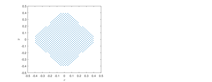
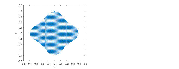
Figure 2: $\mathcal{C}_{6}$ and $\mathcal{C}_{7}$, Example 1

Table 1 shows errors and orders of convergence for the displacement $u$ and the Airy-stress function $v$. Observe that linear order of convergences are obtained for $u$ and $v$ in the energy norm, and quadratic order of convergence in $L^{\infty}$ norm. These numerical order of convergence in energy norm clearly matches the expected order of convergence given in Theorem 5.1. Though the theoretical rate of convergence in $L^{\infty}$ norm is not analysed, the numerical rates are obtained similar to that in [7] for the biharmonic obstacle problem.

Example 2. (Coincidence set with zero measure) In this example taken from [7], $\chi(\boldsymbol{x})=1-5|\boldsymbol{x}|^{2}-|\boldsymbol{x}|^{4},\boldsymbol{x}\in\Omega=0.5(-1,1)^{2}$ with $\Delta^{2}\chi=-64<0$ in $\Omega$, and hence, the interior of the coincidence set must be empty, since $\Delta^{2}u$ (in the sense of distributions) is a nonnegative measure ([10, Section 8]). This can be observed in the pictures of the discrete coincidence sets displayed in Figure 3.

Table 2: Convergence results for Example 2 on the square domain

$\ell$	$h$	$\widetilde{e}_{\ell}(u)$	EOC	$\widetilde{e}_{\ell}(v)$	EOC	$e_{\ell}(u)$	EOC	$e_{\ell}(v)$	EOC
1	0.5000	0.028792	1.4917	0.136864	1.8793	15.510398	0.7999	1.493256	0.9636
2	0.2500	0.028792	1.8646	0.050539	1.9898	11.837363	0.9024	1.070278	1.0843
3	0.1250	0.009347	1.9451	0.014530	2.0535	7.563740	0.9878	0.510661	1.0899
4	0.0625	0.003116	2.1252	0.003980	2.1462	4.210097	1.0591	0.244868	1.1047
5	0.0312	0.000843	2.3636	0.001030	2.3427	2.138703	1.1411	0.118649	1.1642
6	0.0156	0.000164	-	0.000203	-	0.969687	-	0.052944	-

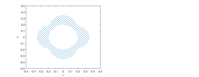
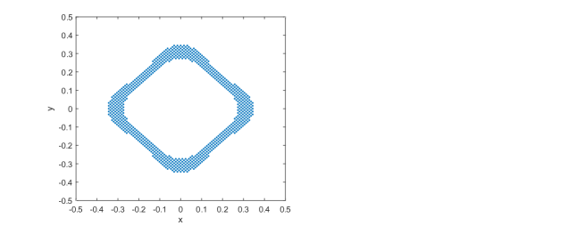
Figure 3: $\mathcal{C}_{6}$ and $\mathcal{C}_{7}$, Example 2

The errors and orders of convergence for the displacement and the Airy-stress function are presented in Table 2. The orders of convergence results are similar to those obtained in Example 1. Note that Examples 1 and 2 are similar except in the sign of the term $|\boldsymbol{x}|^{4}$ that appears in the obstacle function.

Example 3. (Violation of smallness assumption) It is interesting to observe that for $\chi$ and $\Omega$ from Example 1 with the source term $f=(x+3)^{2}(x-3)^{2}(y+3)^{2}(y-3)^{2}$, the primal dual active set algorithm is not convergent in 100 iterations of the algorithm. Consider $w(x,y)=(x+0.5)^{2}(y+0.5)^{2}(0.5-x)^{2}(0.5-y)^{2}\in H^{2}_{0}(\Omega)$. Then $\frac{\|w\|_{L^{2}(\Omega)}}{|\!|\!|w|\!|\!|}=0.0278$ and $\frac{\|w\|_{L^{\infty}(\Omega)}}{|\!|\!|w|\!|\!|}=0.0683$. Since $C_{\rm F}$ (resp. $C_{\rm S}$) is the supremum of $\frac{\|z\|_{L^{2}(\Omega)}}{|\!|\!|z|\!|\!|}$ (resp. $\frac{\|z\|_{L^{\infty}(\Omega)}}{|\!|\!|z|\!|\!|}$) for all $z\in H^{2}_{0}(\Omega)$, this implies $C_{\rm F}\geq 0.0278$ (resp. $C_{\rm S}\geq 0.0683$). Use the definition of $M(f,\chi)$ to obtain $C_{S}M(f,\chi)\geq 20.7972$. Therefore the sufficient condition in Theorem 5.1 is violated.

For Example 1 with obstacle $\chi$ replaced by $\lambda\chi$, where $\lambda\in\mathbb{R}$, we noticed that the algorithm fails to converge for $\lambda\geq 4$ on $\mathcal{T}_{4}$ and $\mathcal{T}_{5}$. This illustrates the requirement of smallness assumption on the obstacle for optimal convergence rate.

6.3 The von Kármán obstacle problem on the L-shaped domain

Consider L-shaped domain $\Omega=(-0.5,0.5)^{2}\setminus[0,0.5]^{2}$, $f=0$ and

$$\chi(\boldsymbol{x})=1-\frac{(x+0.25)^{2}}{0.2^{2}}-\frac{y^{2}}{0.35^{2}}$$

as in [7]. Choosing the initial mesh size as $h=0.7071$, the successive red-refinement algorithm computes $\mathcal{T}_{1},\dots,\mathcal{T}_{5}$.

Table 3: Convergence results for the L-shaped domain

$\ell$	$h$	$\widetilde{e}_{\ell}(u)$	EOC	$\widetilde{e}_{\ell}(v)$	EOC	$e_{\ell}(u)$	EOC	$e_{\ell}(v)$	EOC
1	0.3536	0.046700	0.8276	0.141271	1.8003	23.203954	0.7177	2.260261	0.9584
2	0.1768	0.021021	0.7196	0.056794	1.9621	18.313668	0.8431	1.530842	1.0905
3	0.0884	0.025796	1.2271	0.017919	2.1111	11.746209	0.9442	0.761967	1.1324
4	0.0442	0.014152	1.5879	0.004655	2.2774	6.556709	1.0473	0.352575	1.1531
5	0.0221	0.004708	-	0.000960	-	3.172522	-	0.158538	-

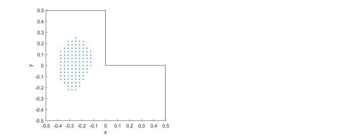
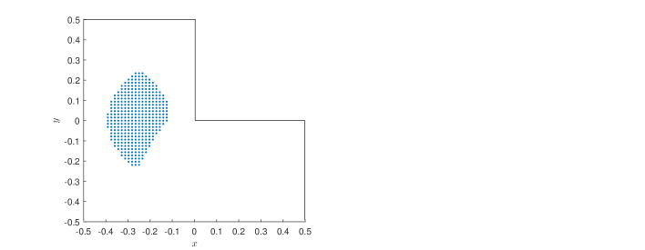
Figure 4: $\mathcal{C}_{5}$ and $\mathcal{C}_{6}$

Since $\Omega$ is non-convex (reduced elliptic regularity $\alpha=0.5445$, [7, Example 4]), we expect only sub-optimal order of convergences in energy norm and $L^{\infty}$ norm, that is, $\mathcal{O}(h^{\alpha})$ convergence rate in the energy norm (see, Theorem 5.1). However, linear order of convergence is preserved in the energy norm which indicates that the numerical performance is carried out in the non-asymptotic region. The discrete coincidence sets for last two levels are depicted in Figure 4. The non-coincidence set is connected, which agrees with the result in [10] since $\Delta^{2}\chi=0$ in $\Omega$ in this example.

The convergence rates in Table 3 are not in direct contradiction to Theorem 5.1 but the reduced elliptic regularity suggests a lower rate $\alpha=0.5445$ for L-shaped domain. A similar observation is in [7, Table 5.5] with orders of convergence $\approx$ 0.8 (resp. 1) for energy (resp. $L^{\infty}$) norm. In [7], the numbers are computed with the alternative definitions for error $e_{\ell}(u):=|\!|\!|u_{\ell-1}-u_{\ell}|\!|\!|_{\text{pw}}$ (resp. $\widetilde{e}_{\ell}(u):=\max_{p\in\mathcal{V}_{\ell-1}}|u_{\ell-1}(p)-u_{\ell}(p)|$) and order of convergence ${\rm{EOC(\ell)}}:={\rm{log}}\big{(}{e_{\ell-1}(u)}/{e_{\ell}(u)}\big{)}/{\rm{log}}(2)$ (resp. ${\rm{log}}\big{(}{\widetilde{e}_{\ell-1}(u)}/{\widetilde{e}_{\ell}(u)}\big{)}/{\rm{log}}(2)$). With these definitions, undisplayed numerical experiments confirm the numbers displayed in [7, Table 5.5] precise up to the last digit. This numerical experiment suggests that our implementation is at least consistent with the one in [7]. One possible explanation is that the corner singularity affects the asymptotic convergence rate for very small mesh-sizes only. This is known, for instance, for the L-shaped domain and the Poisson model problem with constant right hand side in the Courant ($\mathcal{P}_{1}$ conforming) finite element method. The expected rate 2/3 is visible only beyond $2\times 10^{6}$ triangles with far better empirical convergence rates before that.

6.4 Conclusions

The numerical results for the Morley FEM in the von Kármán obstacle problem are presented for square domain and L-shaped domain in Sections 6.2 and 6.3. The outputs obtained for the square domain confirm the theoretical rates of convergence given in Theorem 5.1 for $\alpha=1$. Example 3 in Section 6.3 illustrates the requirement of smallness assumption on the obstacle for optimal convergence rate. For the L-shaped domain, we expect reduced convergence rates in energy and $L^{\infty}$ norms from the elliptic regularity. However, linear order of convergence is preserved in the energy norm which indicates that the numerical performance is carried out in the non-asymptotic region.

Acknowledgements. The authors thankfully acknowledge the support from the MHRD SPARC project (ID 235) titled "The Mathematics and Computation of Plates" and the second to fifth authors also thank the hospitality of the Humboldt-Universität zu Berlin for the corresponding periods 1st June 2019-31st August 2019 (second and fifth authors), 24th June 2019-30th June 2019 (third author), and 1st July 2019-31st July 2019 (fourth author).

References

- [1] Constantin Bacuta, James H. Bramble, and Joseph E. Pasciak. Shift theorems for the biharmonic Dirichlet problem. In Recent Progress in Computational and Applied PDEs, pages 1–26. Springer, 2002.
- [2] Melvyn S. Berger and Paul C. Fife. Von Kármán equations and the buckling of a thin elastic plate, II plate with general edge conditions. Communications on Pure and Applied Mathematics, 21(3):227–241, 1968.
- [3] Heribert Blum and Rolf Rannacher. On mixed finite element methods in plate bending analysis. Computational Mechanics, 6(3):221–236, 1990.
- [4] Heribert Blum, Rolf Rannacher, and Rolf Leis. On the boundary value problem of the biharmonic operator on domains with angular corners. Mathematical Methods in the Applied Sciences, 2(4):556–581, 1980.
- [5] Susanne C. Brenner, Michael Neilan, Armin Reiser, and Li-Yeng Sung. A interior penalty method for a von Kármán plate. Numerische Mathematik, 135(3):803–832, 2017.
- [6] Susanne C. Brenner, Li-Yeng Sung, Hongchao Zhang, and Yi Zhang. A quadratic interior penalty method for the displacement obstacle problem of clamped Kirchhoff plates. SIAM Journal on Numerical Analysis, 50(6):3329–3350, 2012.
- [7] Susanne C. Brenner, Li-Yeng Sung, Hongchao Zhang, and Yi Zhang. A Morley finite element method for the displacement obstacle problem of clamped Kirchhoff plates. Journal of Computational and Applied Mathematics, 254:31–42, 2013.
- [8] Susanne C. Brenner, Li-Yeng Sung, and Yi Zhang. Finite element methods for the displacement obstacle problem of clamped plates. Mathematics of Computation, 81(279):1247–1262, 2012.
- [9] Franco Brezzi. Finite element approximations of the von Kármán equations. RAIRO. Analyse Numérique, 12(4):303–312, 1978.
- [10] Luis A. Caffarelli and Avner Friedman. The obstacle problem for the biharmonic operator. Annali della Scuola Normale Superiore di Pisa-Classe di Scienze, 6(1):151–184, 1979.
- [11] Carsten Carstensen, Dietmar Gallistl, and Jun Hu. A discrete Helmholtz decomposition with Morley finite element functions and the optimality of adaptive finite element schemes. Computers and Mathematics with Applications, 68(12):2167–2181, 2014.
- [12] Carsten Carstensen, Gouranga Mallik, and Neela Nataraj. A priori and a posteriori error control of discontinuous Galerkin finite element methods for the von Kármán equations. IMA Journal of Numerical Analysis, 39(1):167–200, 2019.
- [13] Carsten Carstensen, Gouranga Mallik, and Neela Nataraj. Nonconforming finite element discretization for semilinear problems with trilinear nonlinearity. IMA Journal of Numerical Analysis, 2020.
- [14] Carsten Carstensen and Neela Nataraj. Adaptive Morley FEM for the von Kármán equations with optimal convergence rates. arXiv preprint arXiv:1908.08013, 2020.
- [15] Carsten Carstensen and Sophie Puttkammer. How to prove the discrete reliability for nonconforming finite element methods. Journal of Computational Mathematics, 38(1):142–175, 2020.
- [16] Philippe G. Ciarlet. The finite element method for elliptic problems. North-Holland Publishing Co., Amsterdam-New York-Oxford, 1978. Studies in Mathematics and its Applications, Vol. 4.
- [17] Philippe G. Ciarlet. Mathematical Elasticity: Volume II: Theory of Plates, volume 27. Elsevier, 1997.
- [18] Jens Frehse. Zum Differenzierbarkeitsproblem bei Variationsungleichungen höherer Ordnung. Abhandlungen aus dem Mathematischen Seminar der Universität Hamburg, 36(1):140–149, 1971.
- [19] Dietmar Gallistl. Morley finite element method for the eigenvalues of the biharmonic operator. IMA Journal of Numerical Analysis, 35(4):1779–1811, 2014.
- [20] Roland Glowinski. Lectures on numerical methods for non-linear variational problems. Springer Science & Business Media, 2008.
- [21] Michael Hintermüller, Kazufumi Ito, and Karl Kunisch. The primal-dual active set strategy as a semismooth Newton method. SIAM Journal on Optimization, 13(3):865–888, 2002.
- [22] David Kinderlehrer and Guido Stampacchia. An introduction to variational inequalities and their applications, volume 31. SIAM, 1980.
- [23] George H. Knightly. An existence theorem for the von Kármán equations. Archive for Rational Mechanics and Analysis, 27(3):233–242, 1967.
- [24] Gouranga Mallik and Neela Nataraj. Conforming finite element methods for the von Kármán equations. Advances in Computational Mathematics, 42(5):1031–1054, 2016.
- [25] Gouranga Mallik and Neela Nataraj. A nonconforming finite element approximation for the von Kármán equations. ESAIM: Mathematical Modelling and Numerical Analysis, 50(2):433–454, 2016.
- [26] E. Miersemann and H. D. Mittelmann. Stability in obstacle problems for the von Kármán plate. SIAM Journal on Mathematical Analysis, 23(5):1099–1116, 1992.
- [27] Tetsuhiko Miyoshi. A mixed finite element method for the solution of the von Kármán equations. Numerische Mathematik, 26(3):255–269, 1976.
- [28] Aliki D. Muradova and Georgios E. Stavroulakis. A unilateral contact model with buckling in von Kármán plates. Nonlinear Analysis: Real World Applications, 8(4):1261–1271, 2007.
- [29] Kunihiko Ohtake, J. Tinsley Oden, and Noboru Kikuchi. Analysis of certain unilateral problems in von Kármán plate theory by a penalty method-part 1. a variational principle with penalty. Computer Methods in Applied Mechanics and Engineering, 24(2):187–213, 1980.
- [30] Kunihiko Ohtake, J. Tinsley Oden, and Noboru Kikuchi. Analysis of certain unilateral problems in von Kármán plate theory by a penalty method-part 2. approximation and numerical analysis. Computer Methods in Applied Mechanics and Engineering, 24(3):317–337, 1980.
- [31] Alfio Quarteroni. Hybrid finite element methods for the von Kármán equations. Calcolo, 16(3):271–288, 1979.
- [32] Laure Reinhart. On the numerical analysis of the von Kármán equations: mixed finite element approximation and continuation techniques. Numerische Mathematik, 39(3):371–404, 1982.
- [33] Shing-Tung Yau and Yang Gao. Obstacle problem for von Kármán equations. Advances in Applied Mathematics, 13(2):123–141, 1992.