Propagator for a driven Brownian particle in step potentials

Abstract

Although driven Brownian particles are ubiquitous in stochastic dynamics and often serve as paradigmatic model systems for many aspects of stochastic thermodynamics, fully analytically solvable models are few and far between. In this paper, we introduce an iterative calculation scheme, similar to the method of images in electrostatics, that enables one to obtain the propagator if the potential consists of a finite number of steps. For the special case of a single potential step, this method converges after one iteration, thus providing an expression for the propagator in closed form. In all other cases, the iteration results in an approximation that holds for times smaller than some characteristic timescale that depends on the number of iterations performed. This method can also be applied to a related class of systems like Brownian ratchets, which do not formally contain step potentials in their definition, but impose the same kind of boundary conditions that are caused by potential steps.

1 Introduction

Diffusion driven by an external force is a paradigmatic example of a stochastic process [1] and has become a testing ground for stochastic thermodynamics in theoretical [2] as well as in experimental studies [3]. Analytically solvable models, however, have remained elusive with only few exceptions like flat potential landscapes with various types of boundary conditions and harmonic potentials. This state of affairs stands in stark contrast to the situation of other more established fields of physics that deal with conceptually similar equations. Every physics undergraduate is taught how to solve the Schrödinger equation for square potentials in order to gain some intuition for systems that behave similarly. The Fokker-Planck equation [4] does, from a mathematical point of view, not differ too much from the one dimensional Schrödinger equation and yet there is no discussion of square potentials or the like to be found that goes beyond the identification of the stationary distribution (provided it exists due to appropriate boundary conditions). In the present work, we will argue that it is indeed worthwhile and feasible to seek for the time-dependent solution of the Fokker-Planck equation with localized initial distribution, i.e., to determine the propagator $p(x,t|x_{\mathrm{init}},t=0)$ in one dimensional systems with forces arising from step potentials. Not only should this close this gap in the literature, it might even prove useful in a more directly applicable sense, since potential steps or correspondingly sharply localized bursts of force could be encountered in systems that exhibit strong entropic barriers [5, 6]. Moreover, we will see in section 5 that even if there is a priori no delta-like force present in a system, certain boundary conditions can be interpreted as if this was the case.

We first fix some notation and state the main objective of this work. We are interested in solving the Fokker-Planck equation

$$\partial_{t}p(x,t)=-\partial_{x}\left(\mu F(x)-D\partial_{x}\right)p(x,t)$$ (1)

for the probability distribution $p(x,t)$ of a particle with mobility $\mu$ and diffusion coefficient $D=\mu k_{\mathrm{B}}T$ with forces of the form

$$F(x)=f_{0}-\sum_{i=1}^{N}\Delta V_{i}\delta(x-x_{i})$$ (2)

arising from a driving force $f_{0}$ and a potential with $N$ steps at arbitrary positions $x_{i}$ and individual step heights of $\Delta V_{i}$. The initial distribution is assumed to be localized at some point $x_{\mathrm{init}}$, i.e., $p(x,t=0)=\delta(x-x_{\mathrm{init}})$. In order to limit the number of parameters to a bare minimum, we use reduced units. Quantities with the dimension of a length are given as multiples of some characteristic length scale $\Delta x$ present in the system, e.g., the distance between two specific potential steps. Time-like quantities are expressed in multiples of the diffusion time $\tau\equiv\Delta x^{2}/D$ and energies in multiples of the thermal energy $k_{\mathrm{B}}T$. Using this set of units, $\Delta x$, $D$, and $\mu$ are set to unity, leading to the Fokker-Planck equation of the form $\partial_{t}p(x,t)=-\partial_{x}j(x,t)$ with the probability current defined as

$$j(x,t)=(F(x)-\partial_{x})p(x,t)\,.$$ (3)

The remainder of this work is structured as follows. In section 2, we derive the boundary conditions for the time-dependent probability distributions on either side of a potential step from first principles. In section 3, a method for constructing the propagator following these boundary conditions is introduced and subsequently applied to a system with a single potential step and free boundary conditions. This results in an analytical expression for the propagator in this system. We extend the scope to systems with an arbitrary number of potential steps and periodic boundary conditions in section 4. As an example with relevance in physics, in section 5 we discuss the propagator in the Brownian ratchet model that is used to describe translocation of stochastically moving strands through pores [7, 8, 9].

2 Boundary Conditions

For a single potential step, we expect, in analogy to the quantum mechanical counterpart, that the time-dependent solution $p(x,t)$ is smooth everywhere except for the position of the potential step $x_{1}$ and jumps at $x_{1}$, thus giving rise to the piecewise defined solution

$$p(x,t)=\left\{\begin{array}[]{ll}p_{1}(x,t)&\mathrm{for}\,x<x_{1}\\ p_{2}(x,t)&\mathrm{for}\,x>x_{1}\end{array}\right.\,.$$ (4)

The time-dependent probability distributions within these half axes, which in view of later generalizations will be called segments, are connected by boundary conditions that are influenced by the step height. In this section, we derive these boundary conditions from first principles.

The Fokker-Planck equation is a continuity equation for the probability density. It describes how probability is redistributed over time and the probability current $j(x,t)$ quantifies the amount of probability passing through a point $x$ at time $t$. This interpretation should remain valid if the potential is discontinuous at $x$, since in reality the discontinuity is just a steep rise in potential. For this reason, the probability current should not be discontinuous even if the potential jumps at some point.

An immediate consequence of a continuous probability current across potential steps is that the left- and right- sided limits of the current have to agree when approaching the step position, i.e.,

$$\lim_{x\nearrow x_{1}}j(x,t)=\lim_{x\searrow x_{1}}j(x,t)\,.$$ (5)

Within each interval, the current is given by (3) with only the constant force present. Therefore, eq. (5) translates into a boundary condition for $p(x,t)$ and its spatial derivative

$$f_{0}p_{1}(x_{1},t)-\partial_{x}p_{1}(x,t)|_{x=x_{1}}=f_{0}p_{2}(x_{1},t)-\partial_{x}p_{2}(x,t)|_{x=x_{1}}\,.$$ (6)

A further boundary condition that involves the characteristics of the potential step can be derived by inverting the relation between current and probability density. For, if the current $j(x,t)$ is known at some time $t$, the probability density can be reconstructed through integration of eq. (3) via the relation

$$p(x^{\prime},t)e^{W(x,x^{\prime})}=p(x,t)-\int_{x}^{x^{\prime}}e^{W(x,x^{\prime\prime})}j(x^{\prime\prime},t)\,\mathrm{d}x^{\prime\prime}\,,$$ (7)

where we denote the work needed for the transition from $x$ to $x^{\prime}$ as

$$W(x,x^{\prime})\equiv-\int_{x}^{x^{\prime}}F(x^{\prime\prime})\,\mathrm{d}x^{\prime\prime}\,.$$ (8)

We now consider the limit of eq. (7) for $x\rightarrow x^{\prime}$ with $x<x_{1}<x^{\prime}$. The integral on the right hand side is of order $\mathcal{O}(x^{\prime}-x)$ and the limit of the work from $x$ to $x^{\prime}$ is just the height $\Delta V$ of the potential step. Therefore, this limit yields

$$p_{1}(x_{1},t)=p_{2}(x_{1},t)e^{\Delta V}\,.$$ (9)

Equation (9) implies that the potential step causes a step in the opposite direction for the probability, which a posteriori is not too surprising considering that a stationary Boltzmann-distribution in a periodic square potential will show exactly this behavior. The crucial point is that this boundary condition holds for a non-stationary dynamics as well. Since the Fokker-Planck equation contains spatial derivatives up to second order, boundary conditions for the probability density (eq. (9)) and first derivative (eq. (5)) are sufficient to determine the evolution of the probability density uniquely.

It is interesting to note that this treatment can be applied in the reverse direction. If, for whatever reason, it is known that the probability density jumps at a specific point by some factor and the probability current is continuous, this behavior can be interpreted as if there was a potential step present at this point. This is similar to the treatment of resetting events that can also be expressed within the formalism of Fokker-Planck equations by augmenting the equation with terms representing the resetting [10, 11, 12, 13].

3 Single Potential Step

As we will see in later sections, solving the Fokker-Planck equation piecewise with boundary conditions given in eq. (6) and (9) can prove quite challenging in the case of arbitrary step positions while a driving force is applied. In order to introduce the key element of the solution technique, it is instructive to start with the simplest model, i.e., a single potential step $\Delta V$ without a driving force and subject to free boundary conditions at infinity, i.e., pure relaxation. Without loss of generality, we assume that the step is located at $x_{1}=0$ and that the distribution is initially localized at some point $x_{\mathrm{init}}<0$.

3.1 Pure relaxation

For $f=0$, the Fokker-Planck equation on the two halves of the real axis can be solved with the ansatz

$$p_{1}(x,t) =\frac{1}{2\sqrt{\pi t}}e^{-\frac{(x-x_{\mathrm{init}})^{2}}{4t}}+\frac{A}{2\sqrt{\pi t}}e^{-\frac{(x+x_{\mathrm{init}})^{2}}{4t}}\equiv\frac{1}{2\sqrt{\pi t}}\int_{-\infty}^{\infty}q_{1}(x^{\prime})e^{-\frac{(x-x^{\prime})^{2}}{4t}}\,\mathrm{d}x^{\prime}$$

$$p_{2}(x,t) =\frac{B}{2\sqrt{\pi t}}e^{-\frac{(x-x_{\mathrm{init}})^{2}}{4t}}\equiv\frac{1}{2\sqrt{\pi t}}\int_{-\infty}^{\infty}q_{2}(x^{\prime})e^{-\frac{(x-x^{\prime})^{2}}{4t}}\,\mathrm{d}x^{\prime}\,,$$ (10)

where $A$ and $B$ are constants yet to be determined.

For $x<0$, the time evolution looks as if there was a mirror image of the initial distribution present on the opposing side of the step. On the positive half of the real axis, the probability distribution evolves like coming from a localized initial condition, albeit with an modified amplitude. These virtual initial distributions $q_{1}$ and $q_{2}$ are depicted in figure 1.

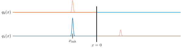
Figure 1: Sketch of the reflection scheme that leads to the analytical solution for the propagator in a system with free boundary conditions and a single potential step at $x_{1}=0$. The initial distribution is reflected at the step position and multiplied by $\tanh(\Delta V/2)$ to obtain the virtual initial distribution for the positive half axis. The virtual initial distribution for the positive half axis is obtained by multiplying the initial distribution with the factor $(1-\tanh(\Delta V/2))$.

An ansatz of this form is suitable, because by placing virtual initial probability at the mirror position of the real initial probability, the ratio of left and right sided probability and its derivative becomes time-independent. Specifically,

$$\frac{p_{1}(0,t)}{p_{2}(0,t)}=\frac{1+A}{B}\quad\mathrm{and}\quad\frac{\partial_{x}p_{1}(x,t)|_{x=0}}{\partial_{x}p_{2}(x,t)|_{x=0}}=\frac{1-A}{B}$$ (11)

for all times. For $f=0$, the boundary conditions (6) and (9) are of the same type as these equations and satisfying them is now a simple matter of solving for the constants $A$ and $B$ with the solution

$$A=h\equiv\tanh(\Delta V/2)\quad\mathrm{and}\quad B=1-h\,.$$ (12)

3.2 Driven Brownian particle

With driving, i.e., $f\neq 0$, the condition of current continuity (5) cannot be fulfilled by the simple ansatz used in section 3.1. In this section we will demonstrate, however, that it is still possible to solve the Fokker-Planck equation and the boundary conditions by introducing virtual initial probability distributions that we denote by $q_{i}(x)$ for both intervals, however of a more involved form than a simple mirror image of the real initial condition with modified amplitude.

In analogy to eq. (10), our ansatz for the propagator reads

$$p_{i}(x,t)=\frac{1}{2\sqrt{\pi t}}\int_{-\infty}^{\infty}q_{i}(x^{\prime})e^{-\frac{(x-x^{\prime}-f_{0}t)^{2}}{4t}}\,\mathrm{d}x^{\prime}\,,$$ (13)

which corresponds to the time evolution of a virtual initial probability distribution $q_{i}(x)$ for each segment $i=1,2$. Note that $q_{i}(x)$ is defined for all real numbers and is not restricted to the interval for which $p_{i}(x,t)$ is defined. Furthermore, the virtual initial distribution does not adhere to the rules normal probability distributions must follow. It does not need to be normalized and can become negative. For the total probability distribution these properties usually are enforced by the boundary conditions connecting the segments to each other and the fact that the distribution is initially normalized and non-negative.

We impose that the $q_{i}(x)$ lead to the correct initial distributions $p_{i}(x,t=0)$, which means that $q_{1}(x)=p_{1}(x,t=0)$ for all $x<0$ and $q_{2}(x)=p_{2}(x,t=0)$ for $x>0$. The segments of $q_{i}(x)$ outside of the respective intervals, here, the other half axis, have to be determined such that the boundary conditions between neighboring segments are respected by the resulting probability distribution.

Using the ansatz

$$q_{i}(x)\equiv g_{i}(x)e^{f_{0}x/2}$$ (14)

for the virtual initial distribution, the time evolution can be rewritten in the form

$$p_{i}(x,t)=\frac{e^{-f_{0}^{2}t/4}}{2\sqrt{\pi t}}\int_{-\infty}^{\infty}g_{i}(x^{\prime})e^{f_{0}x/2}e^{-\frac{(x-x^{\prime})^{2}}{4t}}\,\mathrm{d}x^{\prime}=c(t)\int_{-\infty}^{\infty}g_{i}(z+x)e^{f_{0}x/2}e^{-\frac{z^{2}}{4t}}\,\mathrm{d}z$$ (15)

with the time-dependent prefactor $c(t)\equiv{e^{-f_{0}^{2}t/4}}/{2\sqrt{\pi t}}$ and $z\equiv x-x^{\prime}$. By splitting the integration interval at zero and substituting $u\equiv z^{2}$, eq. (15) can be rewritten in terms of a Laplace transformation

$$p_{i}(x,t) =c(t)e^{f_{0}x/2}\int_{0}^{\infty}\frac{1}{2\sqrt{u}}\left(g_{i}(x+\sqrt{u})+g_{i}(x-\sqrt{u})\right)e^{-\frac{u}{4t}}\mathrm{d}u$$ (16)

$$=c(t)e^{f_{0}x/2}\mathcal{L}_{u}\left[\bar{g}_{i}(x,\sqrt{u})/\sqrt{u}\right]\left(\frac{1}{4t}\right)\,.$$

We use the notation

$$\mathcal{L}_{u}[f(u)](z)\equiv\int_{0}^{\infty}f(u)e^{-zu}\mathrm{d}u$$ (17)

and we introduce the symmetric part of $g_{i}(z)$ with respect to $x$ as

$$\bar{g}_{i}(x,z)\equiv(g_{i}(x+z)+g_{i}(x-z))/2\,.$$ (18)

Along similar lines, the spatial derivative of the distribution can be expressed as

$$\partial_{x}p_{i}(x,t)=c(t)e^{f_{0}x/2}\mathcal{L}_{u}\left[\left(\partial_{x}\bar{g}_{i}(x,\sqrt{u})+\frac{f_{0}}{2}\bar{g}(x,\sqrt{u})\right)/\sqrt{u}\right]\left(\frac{1}{4t}\right)$$ (19)

Due to the uniqueness of the Laplace transformation, the boundary conditions (9) and (5) that must hold for all times transform into conditions on $\bar{g}_{i}(x,z)$ that must hold for all $z$, i.e.,

$$\bar{g}_{1}(x_{1},z)=e^{\Delta V}\bar{g}_{2}(x_{1},z)$$ (20)

and

$$\frac{f_{0}}{2}\bar{g}_{1}(x_{1},z)-\partial_{x}\bar{g}_{1}(x,z)|_{x=x_{1}}=\frac{f_{0}}{2}\bar{g}_{2}(x_{1},z)-\partial_{x}\bar{g}_{2}(x,z)|_{x=x_{1}}\,.$$ (21)

Initially, the functions $g_{i}(x)$ are known only on the respective half axis where they have to correspond to $p(x,t)$, so for equations (20) and (21) to be useful, they have to be rewritten such that they allow the calculation of $g_{i}(x)$ on the other half axis. It turns out that this goal can be achieved by assuming that the functions $g_{1}(x_{1}-z)$ and $g_{2}(x_{1}+z)$ are known for positive $z$ and solving for the yet unknown $g_{1}(x_{1}+z)$ and $g_{2}(x_{1}+z)$. This scheme leads to the uncoupled inhomogeneous differential equations

$$g^{\prime}_{1}(x_{1}+z)-\frac{f_{0}h}{2}g_{1}(x_{1}+z)=\psi(z)$$ (22)

and

$$g^{\prime}_{2}(x_{1}-z)+\frac{f_{0}h}{2}g_{2}(x_{1}-z)=\phi(z)$$ (23)

with the inhomogeneous terms

$$\psi(z)\equiv\frac{hf_{0}}{2}g_{1}(x_{1}-z)-hg^{\prime}_{1}(x_{1}-z)+(1+h)g^{\prime}_{2}(x_{1}+z)$$ (24)

and

$$\phi(z)\equiv-\frac{hf_{0}}{2}g_{2}(x_{1}+z)+hg^{\prime}_{2}(x_{1}+z)+(1-h)g^{\prime}_{1}(x_{1}-z)\,,$$ (25)

respectively. These can be readily solved by integration provided the unknown functions are known for one reference point $x_{\mathrm{s}}$. Thus we have found the desired linear operations that replace the act of reflecting the initial probability density in the case of non-vanishing driving force, namely

$$g_{1}(x)=\hat{S}^{+}(x_{\mathrm{s}})\left(\begin{array}[]{c}g_{1}(x)\\ g_{2}(x)\end{array}\right)\equiv g_{1}(x_{\mathrm{s}})e^{hf_{0}(x-x_{\mathrm{s}})/2}+\int_{x_{\mathrm{s}}}^{x}e^{-hf_{0}(x^{\prime}-x)/2}\,\psi(x^{\prime}-x_{1})\,\mathrm{d}x^{\prime}$$ (26)

and

$$g_{2}(x)=\hat{S}^{-}(x_{\mathrm{s}})\left(\begin{array}[]{c}g_{1}(x)\\ g_{2}(x)\end{array}\right)\equiv g_{2}(x_{\mathrm{s}})e^{-hf_{0}(x-x_{\mathrm{s}})/2}+\int_{x_{\mathrm{s}}}^{x}e^{+hf_{0}(x^{\prime}-x)/2}\,\phi(x_{1}-x^{\prime})\,\mathrm{d}x^{\prime}\,.$$ (27)

Of course, the rescaled virtual initial distributions appear on both sides of eqs. (26) and (27) and so at first glance they only seem to express a self consistency relation between the two functions. The operators $\hat{S}^{\pm}$ are, however, constructed in such a way that they can be evaluated if only parts of the functions are known. If the driving force vanishes, the integrations eqs. (26) and (27) become a simple reflection and thus reproduce the result for this case we discussed above, as it is to be expected.

For a single potential step with driving force $f\neq 0$ the situation is as follows: Since the initial distribution is known, we have $q_{1}(x)=\delta(x-x_{\mathrm{init}})$ for $x\leq 0$, and $q_{2}(x)=0$ for $x\geq 0$. These known function parts correspond to the blue intervals shown in figure 1. The unknown parts, i.e., $q_{1}(x)$ for $x>0$ and $q_{2}(x)$ for $x<0$ can be obtained using the integration scheme (26) and (27), respectively, with the reference value $x_{\mathrm{s}}=0$ and $q_{1}(0)=q_{2}(0)=0$ is already known from the initial condition.

Performing the integrals and reversing eq. (14) yields

$$q_{1}(x)=\delta(x-x_{\mathrm{init}})+he^{-f_{0}x_{\mathrm{init}}}\delta(x+x_{\mathrm{init}})+\theta(x+x_{\mathrm{init}})\frac{f_{0}}{2}e^{f_{0}\left[h(x+x_{\mathrm{init}})+x-x_{\mathrm{init}}\right]/2}\left(h^{2}+h\right)$$ (28)

and

$$q_{2}(x)=(1-h)\delta(x-x_{\mathrm{init}})+\theta(x_{\mathrm{init}}-x)f_{0}e^{f_{0}\left[h(x_{\mathrm{init}}-x)+x-x_{\mathrm{init}}\right]/2}\left(h^{2}-h\right)/2$$ (29)

The time evolution of these virtual initial distributions according to eq. (13) yields the exact propagator for driven diffusion over a single potential step, which constitutes one of our main results. We obtain

$$p(x<0,t|x_{\mathrm{init}},0)=\frac{1}{2\sqrt{\pi t}}e^{-{(x-x_{\mathrm{init}}-f_{0}t)^{2}}/{4t}}+\frac{he^{-f_{0}x_{\mathrm{init}}}}{2\sqrt{\pi t}}e^{-{(x+x_{\mathrm{init}}-f_{0}t)^{2}}/{4t}}$$

$$\!\!\qquad\quad+\frac{f_{0}e^{f_{0}x_{\mathrm{init}}h}}{4}\left(h^{2}+h\right)\left(\mathop{\mathrm{erf}}\left(\frac{f_{0}th+x+x_{\mathrm{init}}}{2\sqrt{t}}\right)+1\right)e^{{f_{0}}(x-x_{\mathrm{init}})(1+h)/{2}-{f_{0}^{2}t}(1-h^{2})/{4}}$$ (30)

and

$$p(x>0,t|x_{\mathrm{init}},0)=\frac{1-h}{2\sqrt{\pi t}}e^{-{(x-x_{\mathrm{init}}-f_{0}t)^{2}}/{4t}}$$

$$\qquad\quad+\frac{f_{0}}{4}(h-h^{2})\left(\mathop{\mathrm{erf}}\left(\frac{f_{0}th-x+x_{\mathrm{init}}}{2\sqrt{t}}\right)+1\right)e^{{f_{0}}(x-x_{\mathrm{init}})(1-h)/{2}-{f_{0}^{2}t}(1-h^{2})/{4}}\,.$$ (31)

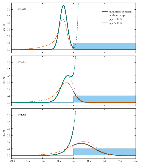
Figure 2: Propagator in a potential landscape with a single step of height $\Delta V=1$ located at $x_{1}=0$ and driving force $f=2$ to the right for different times. Shown are the time evolutions of the virtual initial probabilities for the left and right half axis (green and orange) in comparison to results obtained by numerical integration of the Fokker-Planck equation and the propagator that would hold if the potential step were not present (dotted). The virtual distributions are drawn as solid lines in regions where they correspond to the propagator and as dashed lines everywhere else. The analytical solutions shows excellent agreement with the numerical one. Comparing with the bare diffusion/drift case, the step leads to a delay of the peak position of the distribution and to broadening.

The time evolution for parameters $f_{0}=2$ and $\Delta V=1$ is shown in figure 2 together with the results of a numerical solution and the solution one expects without a potential step, i.e., for $\Delta V=0$. For small times, when no significant portions of the distribution have reached the step yet, the distribution looks Gaussian, as is to be expected. When the broadening distribution reaches the step, parts of it are reflected, leading to a diminished probability current when compared to the free solution. This leads to the formation of a inflection point in the probability distribution, as it is shown in the middle panel of figure 2. In the course of time most of the distribution crosses the barrier and the distribution almost regains its Gaussian shape on the positive half axis, although the distribution is slightly asymmetric with a longer tail on the left than on the right. On the left half axis, the distribution transforms into an almost exponential one, which corresponds to the stationary distribution if the potential step was infinitely high (c.f. bottom panel). For even longer times, not shown in figure 2, all probability eventually crosses the potential barrier and the time evolution of eq. (31) (orange curves) covers the full propagator in the long time limit.

3.3 Reflecting and absorbing boundary conditions

If the height of the potential step diverges, transitions across the step position $x_{1}$ are possible only in one direction depending on the sign of $\Delta V$. We can exploit this correspondence to determine the propagator of a driven Brownian particle confined to the negative half axis, i.e., with reflecting boundary conditions at $x_{1}=0$. This boundary condition corresponds to $\Delta V\rightarrow\infty$ leading to $h=1$ in eq. (30) that now simplifies to

$$p_{\mathrm{ref.}}(x,t|x_{\mathrm{init}},0) =\frac{1}{2\sqrt{\pi t}}e^{-{(x-x_{\mathrm{init}}-f_{0}t)^{2}}/{4t}}+\frac{e^{-f_{0}x_{\mathrm{init}}}}{2\sqrt{\pi t}}e^{-{(x+x_{\mathrm{init}}-f_{0}t)^{2}}/{4t}}$$ (32)

$$\qquad\quad+\frac{f_{0}}{2}\left(\mathop{\mathrm{erf}}\left(\frac{f_{0}t+x+x_{\mathrm{init}}}{2\sqrt{t}}\right)+1\right)e^{{f_{0}}x}$$

for $x<0$. In the long-time limit the first two terms vanish and the third converges to $p_{\mathrm{eq}}(x)=f_{0}e^{f_{0}x}$ for positive $f_{0}$, i.e., to the Boltzmann-distribution, as it is to be expected.

If we have $\Delta V\rightarrow-\infty$ instead, no transitions are allowed from the positive to the negative half axis while transitions in the opposing direction are allowed. If the initial distribution is solely located on the negative half axis, these boundary conditions have the same effect on the negative half axis as absorbing boundary conditions. When inserting $h=-1$ into (30) one obtains

$$p_{\mathrm{abs.}}(x,t|x_{\mathrm{init}},0)=\frac{1}{2\sqrt{\pi t}}e^{-{(x-x_{\mathrm{init}}-f_{0}t)^{2}}/{4t}}-\frac{e^{-f_{0}x_{\mathrm{init}}}}{2\sqrt{\pi t}}e^{-{(x+x_{\mathrm{init}}-f_{0}t)^{2}}/{4t}}\\$$ (33)

for $x<0$.

4 Multiple potential steps

In contrast to a single step with free boundary conditions, an arbitrary number of steps with possibly periodic boundary conditions, i.e., effectively an infinite number of repeating steps, poses additional challenges to the reflection scheme we introduced in section 3. In this section, we will present a more generalized strategy to calculate an approximation to the propagator for these systems.

4.1 Method of reflected probability

When dealing with multiple potential steps, it is reasonable to split the propagator at the positions of steps in the potential landscape. By using an ansatz of the form

$$p(x,t)=\left\{\begin{array}[]{ll}p_{1}(x,t)&\mathrm{for}\,x\in(x_{0},x_{1})\\ p_{2}(x,t)&\mathrm{for}\,x\in(x_{1},x_{2})\\ \cdots\\ p_{i}(x,t)&\mathrm{for}\,x\in(x_{i-1},x_{i})\\ \cdots\\ p_{N+1}(x,t)&\mathrm{for}\,x\in(x_{N},x_{N+1})\end{array}\right.\,,$$ (34)

where $x_{0}$ or $x_{N+1}$ might formally be set to positive or negative infinity to indicate free boundary conditions. The boundary conditions connecting one such segment $p_{i}(x,t)$ to its neighbors can be derived in the same way as it was performed for the single step in section 2. The only difference is that the resulting set of conditions take into account the properties of the individual potential step, i.e., the position $x_{i}$ and the step height $\Delta V_{i}$.

As it was the case for the single step in section 3.3 one could incorporate reflecting or absorbing boundary conditions, by performing the limit $\Delta V_{i}\rightarrow\pm\infty$ at the first or last step position. In any other position, a diverging step corresponds to a boundary that allows transitions only in one direction.

Periodic boundary conditions that may be enforced in addition to the conditions resulting from potential steps are mathematically equivalent to the latter (eqs. (6) and (9)) when setting the step height to zero and using different values at which the respective functions are evaluated on the left- and right-hand side of these equations. This relation between the two types of boundary conditions allows us to treat them both in a unified way by introducing $p_{l(i)}$ and $p_{r(i)}$ for the segments of the propagator to the left or right of the $i$-th potential step and the notation $x_{l(i)}$ and $x_{r(i)}$ for the positions of these two functions that are connected by the condition. The unified boundary conditions read

$$p_{l(i)}(x_{l(i)},t)=p_{r(i)}(x_{r(i)},t)e^{\Delta V_{i}}\,.$$ (35)

and

$$f_{0}p_{l(i)}(x_{l(i)},t)-\partial_{x}p_{l(i)}(x,t)|_{x=x_{l(i)}}=f_{0}p_{r(i)}(x_{r(i)},t)-\partial_{x}p_{r(i)}(x,t)|_{x=x_{r(i)}}\,.$$ (36)

If periodic boundary conditions are enforced, we may for simplicity assume, without loss of generality, that $x$ is confined in the interval $[0,L]$, where $L$ is the period length and that one of the potential steps is situated at the periodic boundary, thus combining the boundary conditions of one step with the periodic boundary condition.

In summary, the propagator is split into segments as shown in figure 3. For free boundaries (top panel), we use an ansatz of the form of eq. (34) with $x_{0}=-\infty$ and $x_{N+1}=\infty$ with $N$ sets of boundary conditions of the form of eq. (35) and eq. (36), where $p_{l(i)}=p_{i}$, $p_{r(i)}=p_{i+1}$, and $x_{l(i)}=x_{r(i)}=x_{i}$. Just as we have seen in section 3.3 it is also possible to incorporate reflecting or absorbing boundary conditions by setting $h_{i}=\pm 1$ on the outermost step positions.

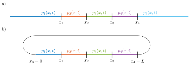
Figure 3: Illustration of step positions and enumeration of the segments $p_{i}(x,t)$ of the propagator in case of free (a) and periodic (b) boundary conditions. Vertical bars mark the positions of potential steps. With free boundary conditions $N$ steps in the potential split the domain in $N+1$ intervals, of which the first and last extend to positive and negative infinity, respectively (top panel). If periodic boundary conditions are imposed (bottom panel), we can, without loss of generality, assume that one potential step is located at the boundary that connects the first and the last segment.

For periodic boundary conditions (bottom panel), we formally have $x_{0}=0$ and $x_{N}=L$ in the ansatz (34) that is now missing the last segment. For all potential steps $i<N$ the boundary conditions are the same as for the free boundary case. For the singular transition $i=N$, we have $p_{l(N)}=p_{N}$, $p_{r(N)}=p_{1}$, $x_{l(i)}=x_{N}$, and $x_{r(i)}=x_{1}$.

After introducing these definitions, we can repeat the same steps that led to the solution of the single step case. In doing so, we introduce the virtual initial distributions corresponding to each segment of the propagator as

$$p_{i}(x,t)=\frac{1}{2\sqrt{\pi t}}\int_{-\infty}^{\infty}q_{i}(x^{\prime})e^{-\frac{(x-x^{\prime}-f_{0}t)^{2}}{4t}}\,\mathrm{d}x^{\prime}=c(t)\int_{-\infty}^{\infty}g_{i}(z+x)e^{f_{0}x/2}e^{-\frac{z^{2}}{4t}}\,\mathrm{d}z\,.$$ (37)

In analogy to the single step, we can compute the unknown parts of the rescaled virtual initial distributions by integrating the differential equations

$$g^{\prime}_{l}(x_{l}+z)-\frac{f_{0}h_{i}}{2}g_{l}(x_{l}+z)=\psi_{l,r}(z)$$ (38)

and

$$g^{\prime}_{r}(x_{r}-z)+\frac{f_{0}h_{i}}{2}g_{r}(x_{r}-z)=\phi_{l,r}(z)$$ (39)

with $h_{i}\equiv\tanh(\Delta V_{i}/2)$. The inhomogeneities read

$$\psi_{l,r}(z)\equiv\frac{h_{i}f_{0}}{2}g_{l}(x_{l}-z)-h_{i}g^{\prime}_{l}(x_{l}-z)+(1+h_{i})e^{f_{0}(x_{r}-x_{l})/2}g^{\prime}_{r}(x_{r}+z)$$ (40)

and

$$\phi_{l,r}(z)\equiv-\frac{h_{i}f_{0}}{2}g_{r}(x_{r}+z)+h_{i}g^{\prime}_{r}(x_{r}+z)+(1-h_{i})e^{f_{0}(x_{r}-x_{l})/2}g^{\prime}_{l}(x_{l}-z)\,,$$ (41)

where we have suppressed the $i$-dependence of $r(i)$ and $l(i)$ for notational simplicity. The solutions are

$$g_{l}(x)=\hat{S}_{i}^{+}(x_{\mathrm{s}})\left(\begin{array}[]{c}g_{l}(x)\\ g_{r}(x)\end{array}\right)\equiv g_{l}(x_{\mathrm{s}})e^{h_{i}f_{0}(x-x_{\mathrm{s}})/2}+\int_{x_{\mathrm{s}}}^{x}e^{-h_{i}f_{0}(x^{\prime}-x)/2}\,\psi_{l,r}(x^{\prime}-x_{l})\,\mathrm{d}x^{\prime}$$ (42)

and

$$g_{r}(x)=\hat{S}_{i}^{-}(x_{\mathrm{s}})\left(\begin{array}[]{c}g_{l}(x)\\ g_{r}(x)\end{array}\right)\equiv g_{r}(x_{\mathrm{s}})e^{-h_{i}f_{0}(x-x_{\mathrm{s}})/2}+\int_{x_{\mathrm{s}}}^{x}e^{+h_{i}f_{0}(x^{\prime}-x)/2}\,\phi_{l,r}(x_{r}-x^{\prime})\,\mathrm{d}x^{\prime}\,,$$ (43)

respectively.

The main difference to the case of a single potential step is that it is no longer possible to calculate the unknown parts of the virtual initial distributions by applying the reflection operators $\hat{S}_{i}^{+}$ and $\hat{S}_{i}^{-}$ once. We rather have to apply them repeatedly, each time generating yet unknown parts of the virtual initial distributions. If, for instance, $g_{l}(x)$ is known in the interval $I_{l}$ and $g_{r}(x)$ is known in the interval $I_{r}$, then the integral in eq. (42) can be evaluated in the interval $\bar{S}_{i}^{+}(I_{r},I_{l})\equiv(2x_{l}-I_{l})\cap(I_{r}-x_{r}+x_{l})$, provided one reference value $g_{l}(x_{\mathrm{s}})$ at the reference position $x_{\mathrm{s}}$ within this interval is known. Equation (43) can be evaluated in the interval $\bar{S}_{i}^{-}(I_{l},I_{r})\equiv(2x_{r}-I_{r})\cap(I_{l}-x_{l}+x_{r})$. In the following, we will demonstrate that the reflection operators $S_{i}^{\pm}$ in conjunction with the initial distribution is sufficient to obtain the propagator in an iterative procedure. This iterative approach is conceptually similar to the problem of finding the electrostatic potential for a charged particle in between two conducting parallel surfaces often discussed in electrodynamics courses, where the method of mirror charges yields a solution in form of an infinite sum [14]. The concrete strategy that has to be employed, however, will depend on the specific potential landscape that is to be studied.

4.2 Two steps with free boundary conditions

To illustrate how to calculate the virtual initial distributions in more complex situations, we first consider the case of a potential landscape with two steps with height $\Delta V_{1}$ and $\Delta V_{2}$ at the positions $x_{1}$ and $x_{2}$, respectively.

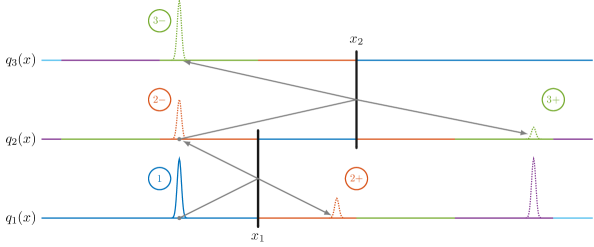
Figure 4: Sketch illustrating the reflection scheme for a potential with two steps placed at $x_{1}$ and $x_{2}$ and initial position placed to the left of $x_{1}$. Each horizontal line represents the virtual initial distribution responsible for a segment of the propagator. The vertical lines correspond to boundary conditions connecting adjacent segments. Initially, the virtual distributions are only known in the intervals where they correspond to the actual initial distribution. These intervals are marked in blue. By repeatedly applying the reflection operators, new parts of the virtual distributions are generated, which are colored in order orange, green, purple, and light blue.

Figure 4 depicts the three virtual initial distributions $q_{i}$ relevant for the intervals $(-\infty,x_{1})$,$(x_{1},x_{2})$, and $(x_{2},\infty)$ as horizontal lines and the potential steps between intervals as vertical bars. Initially, the virtual initial distributions are known only in those intervals for which $q_{i}$ must correspond to the initial distribution. These intervals are marked in blue in the figure. Applying the four operators $S_{i}^{\pm}$ with $i\in\{1,2\}$ corresponding to the boundary conditions at the potential steps one can now obtain parts of adjacent $q_{i}$ (marked in red) in analogy to the case of a single step. In contrast to the single step, however, the initial interval in which $q_{2}$ is known, has a finite length, and therefore the newly calculated parts are limited by that length. To illustrate the procedure figure 4 depicts the case without driving force for which the operators correspond to mere reflections. Here, we find that in this first step the initial delta-peak (marked with 1) gets reflected by $S_{1}^{+}$ to a peak (marked as $2+$) on the other side of the first step position $x_{1}$. Analogously, $S_{1}^{-}$ maps the same peak with different height onto $q_{2}$ (marked as $2-$).

When performing the scheme a second time, the peak $2-$ is reflected by the operators $S_{2}^{\pm}$ with respect to the second step position $x_{2}$ resulting in new peaks on $q_{2}$ and $q_{3}$. The peaks are marked as $3+$ and $3-$, respectively. In each following step, the peak that was generated on $q_{2}$ in the step before, will give rise to a new peak on either $q_{1}$ or $q_{3}$ and a new peak on $q_{2}$ (c.f. purple peak in fig. 4, the new peak on $q_{2}$ lies outside of the depicted interval).

Since each step of this scheme generates parts of the virtual initial distribution only on intervals of finite length, it would have to be repeated infinitely often to obtain the full functions $q_{i}(x)$ for all real numbers. For practical purposes, it is sufficient to stop after a finite number of iterations, which results in an approximation valid for small times. It is, however, necessary to specify how to treat the still unknown parts of the virtual initial distributions when calculating the time evolution according to eq. (37). It turns out that, when driving forces are present, the reflection operators may generate a virtual initial distribution that grows exponentially with $x$ (c.f. eq. (28)). So, naively setting the virtual initial distribution to zero where it is unknown or equivalently limiting the integration in eq. (13) to the known parts of $q_{i}$ will introduce an artificial step in the initial distribution that originates solely from stopping the iteration after finitely many steps. To avoid this step from occurring, we assume instead that the function that describes the last known part of the function remains valid in the unknown intervals. While this is not the correct initial distribution either, we observe that this procedure, called “extension”, converges faster to the real propagator than the naive procedure.

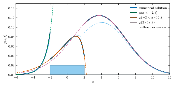
Figure 5: Propagator for an initially localized distribution at $x_{\mathrm{init}}=-5$ driven by a force $f_{0}=2$ in a potential landscape with step $\Delta V_{1}=1$ at $x_{1}=-2$ and step $\Delta V_{2}=-1$ (as indicated by the shaded rectangle) at $x=2$ at time $t=4.52$. The figure shows the piecewise defined approximation obtained by reflecting the initial distribution $N_{\mathrm{it}}=2$ times at the potential steps in comparison to a numerical solution of the Fokker-Planck equation showing excellent agreement despite the fact that the reflection scheme was performed only twice. If the left and rightmost known intervals of the virtual initial distribution are not extended to infinity the approximation becomes worse as is indicated by the dotted lines. Without the extension, the iteration has to be repeated $N_{\mathrm{it}}=4$ times to achieve a match to the numerical solution within error bars that correspond to the thickness of the curve (not shown).

As an example, in Fig. 5, we show the propagator $p(x,t|x=-5,t=0)$ in a system with a rectangular potential barrier of height $\Delta V=1$ between $x=-2$ and $x=2$ for a driving force of $f_{0}=2$.

4.3 Generalization to an arbitrary number of steps

The method discussed for the case of two potential steps can straightforwardly be generalized to the case of an arbitrary number of steps. As before the reflection scheme will lead to an iterative solution. We use the index $k$ to count iterations. At the beginning of the iteration, the virtual distributions are known in the intervals $I_{i}^{0}=[x_{i-1},x_{i}]$. The initial guess for the rescaled virtual initial distribution is

$$g_{i}^{0}(x)=\left\{\begin{array}[]{lc}p(x,t=0)e^{-f_{0}x/2}&\mathrm{for}\,x\in I_{i}^{0}\\ \mathrm{undefined}&\mathrm{otherwise}\end{array}\right.\,.$$ (44)

In each iteration step, one can generate new parts for each $g_{i}$ by applying $\hat{S}_{i}^{+}(x_{\mathrm{s}})$ and $\hat{S}_{i-1}^{-}(x_{\mathrm{s}})$ with a suitable choice for the seam position $x_{\mathrm{s}}$, i.e.,

$$g_{i}^{k+}(x)=\hat{S}_{i}^{+}(x_{\mathrm{s}}^{k+})\left(\begin{array}[]{c}g_{i}^{k}(x)\\ g_{i+1}^{k}(x)\end{array}\right)$$ (45)

and

$$g_{i}^{k-}(x)=\hat{S}_{i-1}^{-}(x_{\mathrm{s}}^{k-})\left(\begin{array}[]{c}g_{i-1}^{k}(x)\\ g_{i}^{k}(x)\end{array}\right)\,.$$ (46)

For practical purposes it is advisable to choose $x_{\mathrm{s}}^{k+}$ as big as possible within the known interval $I_{i}^{k}$ to avoid repeating operations already performed in earlier iterations. For the same reason, $x_{\mathrm{s}}^{k-}$ should be chosen as small as possible.

The new functions $g_{i}^{k\pm}(x)$ generated in the $k$-th step can be evaluated in the intervals $I_{i}^{k+}=\bar{S}_{i}^{+}(I_{i}^{k},I_{i+1}^{k})$ and $I_{i}^{k-}=\bar{S}_{i-1}^{-}(I_{i-1}^{k},I_{i}^{k})$, respectively. These intervals in all but the first step will have overlap with all previously generated intervals but will also contain new parts. Since all generated functions $g_{i}^{k}$ are constructed using the same operators, $g_{i}^{k\pm}$ will agree with the previous iterations in all parts that were already known.

These considerations lead to the updated interval

$$I_{i}^{k+1}=I_{i}^{k}\cup I_{i}^{k+}\cup I_{i}^{k-}.$$ (47)

and the updated approximation of the rescaled virtual initial distribution

$$g_{i}^{k+1}(x)=\left\{\begin{array}[]{ll}g_{i}^{k}(x)&\mathrm{for}\,x\in I_{i}^{k}\\ g_{i}^{k+}(x)&\mathrm{for}\,x\in I_{i}^{k+}\setminus I_{i}^{k}\\ g_{i}^{k-}(x)&\mathrm{for}\,x\in I_{i}^{k-}\setminus I_{i}^{k}\\ \mathrm{undefined}&\mathrm{otherwise}\end{array}\right.\,.$$ (48)

As stated above, excluding $I_{i}^{k}$ from the second and third case would not strictly be necessary since the functions agree anyway. Repeating this iteration scheme and computation of the time evolution according to eq. (37) yields an approximation to the desired propagator.

4.4 An algorithm for a closed form of the propagator

Requiring a large number of consecutive integrations of some functions immediately poses the question, whether it is feasible to arrive at a result in closed form. While this most likely will not be possible for arbitrary initial distributions, we will show in this section that after an arbitrary number of integration steps the virtual initial distribution can be expressed in closed form provided that the initial probability is localized. Thus the propagator can be expressed in closed form. For such an initial condition, the rescaled virtual initial distribution can be expressed in the form

$$g_{i}(x)=\sum_{j}a_{i,j}\delta(x-\tilde{x}_{i,j})+\theta(x-\tilde{x}_{i,j})\left(\sum_{k}\mathcal{P}_{i,j,k}^{+}(x)e^{b_{i,j,k}^{+}x}\right)$$

$$\quad+\theta(\tilde{x}_{i,j}-x)\left(\sum_{k}\mathcal{P}_{i,j,k}^{-}(x)e^{b_{i,j,k}^{-}x}\right)\,,$$ (49)

where $\mathcal{P}^{\pm}_{i,j,k}(x)$ denotes some polynomial of $x$, $\tilde{x}_{i,j}$ are positions of step- or delta-functions, $a_{i,j}$ are the amplitudes of the delta-functions, and $b_{i,j,k}^{\pm}$ are real valued coefficients in the exponential prefactors of the polynomials $\mathcal{P}^{\pm}_{i,j,k}(x)$.

Such an expression holds since the operations necessary to calculate the result of the reflection operators defined in eqs. (42) and (43), can, by means of integration by parts, be broken down into a concatenation of the following operations:

• shifting in $x$: $g_{i}(x)\rightarrow g_{i}(x-c)$

• reflection of $g_{i}(x)$ at some point $c$: $g_{i}(x)\rightarrow g_{i}(2c-x)$

• multiplication with an exponential function: $g_{i}(x)\rightarrow g_{i}(x)\,ae^{cx}$

• integration: $g_{i}(x)\rightarrow\int_{x_{\mathrm{s}}}^{x}g_{i}(x^{\prime})\,\mathrm{d}x^{\prime}$

• addition of multiple functions of the type of eq. (49).

Each of these five operations preserves the form of eq. (49) and can be executed in closed form. Since the initial distribution is also of the same form, this guarantees that an arbitrary number of reflection operations can be performed on the initial distribution while still obtaining a result in closed form, i.e., of the form of eq. (49). While the calculation can become quite tedious, since it involves, among others, recursive integration by parts and application of the binomial theorem, it is possible to create an algorithm for performing these steps using standard computer algebra libraries.

Finally, the explicit calculation of the time evolution of the virtual initial probabilities and, hence, the propagator, is also possible in closed form. A reference implementation of such an algorithm is provided in the supplementary material https://github.com/muhl/StepPotentialPropagator

5 Brownian ratchet as an application

Driven diffusion in potentials with steps or, equivalently, driven diffusion with boundary conditions of the form of eq. (35) and eq. (36) are not only useful as introductory problems to the topic of driven diffusion. They can be encountered, inter alia, in biophysical problems described as Brownian ratchets. In this section, we will derive an approximation for the corresponding propagator using the reflection scheme.

In brief, the Brownian ratchet model originally introduced by Oster and Peskin [16, 17] describes the stochastic dynamics of translocation of a polymer strand through a pore. It is assumed that on one side of the pore molecules can bind to equidistant sites on the strand that will block a retraction of the strand back through the pore. The strand itself undergoes regular diffusion that may be biased by a pulling force. The timescale of the binding and unbinding processes of the bound molecules is assumed to be fast when compared to the diffusion timescale, which means that one can assume that the binding sites are always in chemical equilibrium with their respective environment. Formally, this model corresponds to the ensemble statistics of the distance $x$ of the barrier to the closest binding site on one side of the pore with a Fokker-Planck of the form of eq. (1). This variable may range between $0$ when the binding site is inside the pore to the distance of two binding sites $\Delta x$.

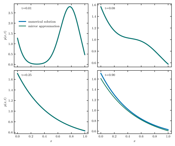
Figure 6: Time evolution of initial distribution localized at $x_{\mathrm{init}}=0.8$ in the Brownian ratchet system with $\Delta x=1$. A pulling force of $f_{0}=-2$ is applied. The probability to reject a transition across the periodic boundary is $1/e$ corresponding to a potential step with height $\Delta V=-1$. The plot compares the numerical integration of the Fokker-Planck equation to the approximation obtained using the reflection method with $N=2$ iterations. We find excellent agreement at early times (top row) and even until the stationary distribution is reached (bottom left). At even larger times the approximation starts to deviate from the numerical solution (bottom right) and is ultimately vanishing for $t\rightarrow\infty$.

Transitions of $x=0$ to $x=\Delta x$ correspond to the transition of a binding site back to the cis side and are therefore rejected with the stationary probability $p_{\mathrm{on}}=w_{\mathrm{bind}}/(w_{\mathrm{bind}}+w_{\mathrm{unbind}})$ of a binding site to be occupied. Transitions in the opposite directions, i.e., the transition of an empty site from the trans to the cis side are always allowed. These modified periodic boundary conditions read

$$\frac{p(0,t)}{p(\Delta x,t)}=1/p_{\mathrm{on}}=e^{-\ln p_{\mathrm{on}}}\,.$$ (50)

To keep the probability distribution normalized at all times, the currents at $x=0$ and $x=\Delta x$ have to match. These boundary conditions are of the same form that arises from the presence of potential steps. Comparison of eq. (50) and eq. (35) shows that the height of the potential step at the periodic boundary can be identified as $\Delta V=\ln p_{\mathrm{on}}$.

The propagator for this system can therefore be calculated with the reflection scheme we discussed above. Because there is only one interval in this case, the virtual initial distribution is obtained by repeatedly processing the single virtual initial distribution with the operators $\hat{S}^{+}$ and $\hat{S}^{-}$ associated with the periodic boundary condition.

As a result the propagator for a initial distribution located at $x=0.8$ is shown in figure 6. We see good agreement between the numerical solution and an approximation with two iterations well beyond the time at which the stationary exponential distribution is reached.

6 Conclusion

In the present work, we have introduced a technique for constructing the propagator in one-dimensional driven stochastic systems with discontinuous potential landscapes. We have demonstrated that it is possible to satisfy the boundary conditions that connect segments of constant potential by calculating the time evolution of virtual initial distributions. This method is conceptually similar to the well known method of images commonly used to solve problems involving conducting surfaces in electrostatics.

While the technique will in all but the simplest example of a single potential step involve an infinite recursion of mirror images, the virtual initial distributions can nevertheless help to gain an intuitive picture of the dynamics. If, as we have seen in section 3, a potential barrier blocks driven diffusion, the actual initial distribution is opposed by a modified mirror image that represents the transitions blocked due to the barrier. Conversely, if a negative step in potential draws probability across the step, the virtual initial distributions may become negative.

It is possible to stop the reflection scheme after a finite number of iterations and still gain a good approximation to the propagator with significantly less computational effort than for a numerical integration of the Fokker-Planck equation. Because the virtual initial distributions are oblivious to periodic boundary conditions, the time evolution predicted by them is unable to attain a non-vanishing stationary state. However, since it is trivial to compute the stationary state [1], a finite number of iterations is sufficient to get an excellent approximation to the propagator for all times, as we were able to demonstrate for the example of a Brownian ratchet.

Further research and optimization could be directed at the open question whether the technique discussed here can be extended into an algorithm suitable for more generic types of potentials. After all, every smooth potential can be approximated by a sequence of potential steps. Preliminary considerations show that the computational effort would scale not worse than established integration schemes, e.g., finite difference approximations to the Fokker-Planck equation [4], with the added benefit that discontinuities in the potential can be handled without the risk of numerical instabilities.

References

References

- [1] Gardiner C 2009 Stochastic Methods: A Handbook for the Natural and Social Sciences 4th ed Springer Series in Synergetics (Berlin Heidelberg: Springer-Verlag) ISBN 978-3-540-70712-7
- [2] Seifert U 2012 Rep. Prog. Phys. 75 126001
- [3] Ciliberto S 2017 Phys. Rev. X 7 021051
- [4] Risken H 1996 Fokker-Planck Equation (Springer Berlin Heidelberg) ISBN 978-3-540-61530-9 978-3-642-61544-3
- [5] Burada P S, Schmid G, Reguera D, Vainstein M H, Rubi J M and Hänggi P 2008 Phys. Rev. Lett. 101 130602
- [6] Kim D, Bowman C, Del Bonis-O’Donnell J T, Matzavinos A and Stein D 2017 Phys. Rev. Lett. 118 048002
- [7] Mahendran K R, Romero-Ruiz M, Schlösinger A, Winterhalter M and Nussberger S 2012 Biophysical Journal 102 39–47
- [8] Hepp C and Maier B 2016 Proc. Natl. Acad. Sci. USA 113 12467–12472
- [9] Uhl M and Seifert U 2018 Phys. Rev. E 98 022402
- [10] Manrubia S C and Zanette D H 1999 Phys. Rev. E 59 4945–4948
- [11] Evans M R and Majumdar S N 2011 Phys. Rev. Lett. 106 160601
- [12] Meylahn J M, Sabhapandit S and Touchette H 2015 Phys. Rev. E 92 062148
- [13] Fuchs J, Goldt S and Seifert U 2016 Europhys. Lett. 113 60009
- [14] Jackson J D 1999 Classical electrodynamics 3rd ed (New York: Wiley) ISBN 978-0-471-30932-1
- [15] \urlhttps://github.com/muhl/StepPotentialPropagator
- [16] Simon S M, Peskin C S and Oster G F 1992 Proc. Natl. Acad. Sci. USA 89 3770–3774
- [17] Peskin C S, Odell G M and Oster G F 1993 Biophys. J. 65 316–324