Exploring the role of new physics in $b\to u\tau\bar{\nu}$ decays

Abstract

The recent measurements on $R_{D}$, $R_{D^{*}}$ and $R_{J/\psi}$ by three pioneering experiments, BaBar, Belle and LHCb, indicate that the notion of lepton flavour universality is violated in the weak charged-current processes, mediated through $b\to c\ell\bar{\nu}_{\ell}$ transitions. These intriguing results, which delineate a tension with their standard model predictions at the level of $(2-3)\sigma$ have triggered many new physics propositions in recent times, and are generally attributed to the possible implication of new physics in $b\to c\tau\bar{\nu}$ transition. This, in turn, opens up another avenue, i.e., $b\to u\tau\bar{\nu}$ processes, to look for new physics. Since these processes are doubly Cabibbo suppressed, the impact of new physics could be significant enough, leading to sizeable effects in some of the observables. In this work, we investigate in detail the role of new physics in $B\to(\pi,\rho,\omega)\tau\bar{\nu}$ and $B_{s}\to(K,K^{*})\tau\bar{\nu}$ processes considering a model independent approach. In particular, we focus on the standard observables like branching fraction, lepton flavour non-universality (LNU) parameter, forward-backward asymmetry and polarization asymmetries. We find significant deviations in some of these observables, which can be explored by the currently running experiments LHCb and Belle-II. We also briefly comment on the impact of scalar leptoquark $R_{2}(3,2,7/6)$ and vector leptoquark $U_{1}(3,1,2/3)$ on these decay modes.

I Introduction

Looking for physics beyond Standard Model (SM) is one of the the prime objectives of present day particle physics research. With no direct evidence of any kind of new physics (NP) signal at the LHC, much attention has been paid in recent times towards the various observed anomalies, which may be considered as smoking-gun signals of NP and require thorough and careful investigation. In this context, semileptonic $B$ decays, both the charged-current $b\to c\ell\bar{\nu}_{\ell}$ as well as neutral-current $b\to s\ell^{+}\ell^{-}$ mediated transitions play a crucial role in probing the nature of physics beyond the SM.

In the last few years, several enthralling anomalies at the level of $(2-4)\sigma$ have been observed by the $B$-physics experiments, i.e., Belle Huschle et al. (2015); Hirose et al. (2017); Abdesselam et al. (2019a, b, c), Babar Lees et al. (2012, 2013) and LHCb Aaij et al. (2013a, b, 2014a, 2014b, 2015a, 2015b, 2017, 2018a, 2018b, 2019), in the form of lepton flavour universality (LFU) violation in semileptonic $B$ decays associated with charged current and neutral current transitions. These discrepancies could be interpreted as hints of lepton flavour universality violation, which can’t be accommodated in the SM and hence, suggest the necessity of NP contributions. In the charged-current sector these observables are characterized by the ratio of branching fractions $R_{D^{(*)}}\equiv{\rm Br}(B\to D^{(*)}\tau\bar{\nu})/{\rm Br}(B\to D^{(*)}\ell\bar{\nu}_{\ell})$, where $\ell=(e,\mu)$ and their present world average values $R_{D}^{\rm exp}=0.340\pm 0.027\pm 0.013$ and $R_{D^{*}}^{\rm exp}=0.295\pm 0.011\pm 0.008$ from Heavy Flavour Averaging Group (HFLAV) Amhis et al. (2019), have $3.1\sigma$ deviation (considering their correlation of $-0.38$) from their corresponding SM values. Analogous observable in the decay of $B_{c}$ meson, symbolized by $R_{J/\psi}=0.71\pm 0.17\pm 0.18$ Aaij et al. (2018b) also exhibits $1.7\sigma$ discrepancy with its SM prediction. Motivated by these results, a legion of studies have been performed from different points of view, e.g., revaluation of form factors in the SM predictions, studies to accommodate $R_{D^{(*)}}$ anomalies in a model-independent way as well as incorporating various NP scenarios and making use of other observables to probe the NP effects, (see for example a representative list Iguro and Watanabe (2020); Blanke et al. (2019); Sahoo and Mohanta (2019); Murgui et al. (2019); Alok et al. (2020); Iguro et al. (2019); Robinson et al. (2019); Sahoo et al. (2017a) and references therein).

The dearth of evidence of similar deviations in semileptonic or leptonic decays of $K$ and $\pi$ mesons, or in electroweak precision observables, supports the idea in which the potential NP contribution responsible for LFU violation is coupled only to the third generation fermions. Thus, for resolving the $R_{D^{(*)}}$ anomalies, it is generally presumed that only $b\to c\tau\bar{\nu}_{\tau}$ decay channel is sensitive to NP. Hence, it is natural to expect that the same class of NP might also affect the related charged current transitions mediated through $b\to u\tau\bar{\nu}_{\tau}$. In this regard, the study of $B\to(\pi,\rho,\omega)\tau\bar{\nu}$ and $B_{s}\to(K,K^{*})\tau\bar{\nu}$ charged current processes, involving the quark level transitions $b\to u\tau\bar{\nu}_{\tau}$ are quite enthralling and in this work, we would like to perform a detailed analysis of these decay modes. Rather than considering any specific NP scenario, we adopt a model-independent approach, wherein we consider all possible Lorentz invariant terms in the effective Lagrangian, describing the process. Using the available experimental data to constrain the possible new coefficients allows us to deduce the information on the nature of NP without any prejudice. We then scrutinize the impact of these new coefficients on the branching fraction, forward-backward asymmetry, LFU observable and lepton polarization asymmetry of these decay modes. It should be emphasized that as these modes are relatively rare due to Cabbibo suppression, the impact of NP could be significant enough leading to observable effects in some of the observables. This in turn, leads the possibility that they could be observed at LHCb or Belle II experiments. Recently, some groups have looked into these decay modes in the context of various new physics scenarios Rajeev and Dutta (2018); Colangelo et al. (2019); Sahoo and Bhol (2020); Colangelo et al. (2020); Kumbhakar and Mohanta (2020).

The outline of the paper is as follows. In Sec. II we present the required theoretical framework to calculate the decay rate and other observables sensitive to NP, starting from the general effective Lagrangian containing new Wilson coefficients. Section-III deals with the constrained parameter space of the new physics couplings. Section-IV is comprised of the effect of NP on various parameters and their sensitivity towards NP. Here we show the $q^{2}$ variation of different observables and compute their numerical values. In Sec. V, we briefly comment on the effect of scalar leptoquark $R_{2}(3,2,7/6)$ and vector leptoquark $U_{1}(3,1,2/3)$ on these observables. Finally, we conclude our work in Section-VI.

II Theoretical Framework

In effective field theory approach, the most general effective Hamiltonian describing the transition $b\to u\tau\bar{\nu}_{\tau}$ is expressed as Sakaki et al. (2013),

$${\cal H}_{eff}=\frac{4G_{F}}{\sqrt{2}}V_{ub}\big{[}(1+V_{L})O_{V_{L}}+V_{R}O_{V_{R}}+S_{L}O_{S_{L}}+S_{R}O_{S_{R}}+T_{L}O_{T_{L}}\big{]},$$ (1)

where $G_{F}$ is the Fermi constant, $V_{ub}$ is the CKM matrix element, $O_{i}$ are the dimension-six four fermion operators and $V_{L},V_{R},S_{L},S_{R},T_{L}$ are the corresponding new Wilson coefficients, which are zero in the SM. Here, we consider the neutrinos as left-chiral. The operator ${\cal O}_{V_{L}}$ corresponds to the SM operator having the usual $(V-A)\times(V-A)$ structure, whereas the other operators $O_{V_{R},S_{L},S_{R},T_{L}}$ arise only in some new physics scenarios. The explicit form of these operators are

$$O_{V_{L}}=(\bar{u}\gamma_{\mu}P_{L}b)(\bar{\tau}\gamma^{\mu}P_{L}\nu),~{}~{}~{}~{}~{}O_{V_{R}}=(\bar{u}\gamma_{\mu}P_{R}b)(\bar{\tau}\gamma^{\mu}P_{L}\nu),~{}~{}~{}~{}~{}O_{S_{L}}=(\bar{u}P_{L}b)(\bar{\tau}P_{L}\nu),$$

$$O_{S_{R}}=(\bar{u}P_{R}b)(\bar{\tau}P_{L}\nu),~{}~{}~{}~{}~{}~{}~{}~{}~{}~{}~{}O_{T_{L}}=(\bar{u}\sigma_{\mu\nu}P_{L}b)(\bar{\tau}\sigma^{\mu\nu}P_{L}\nu),$$ (2)

where $P_{L,R}=(1\mp\gamma_{5})/2$ represent the chiral projection operators.

Including all new physics operators of the effective Hamiltonian (1), the differential decay distribution for the $\bar{B}\to P\tau\bar{\nu}$ processes (where $P$ denotes a psedoscalar meson), can be represented in terms of helicity amplitudes Sakaki et al. (2013)

$$\frac{d\Gamma(\bar{B}\to P\tau\bar{\nu})}{dq^{2}} = {G_{F}^{2}|V_{ub}|^{2}\over 192\pi^{3}m_{B}^{3}}q^{2}\sqrt{\lambda_{P}(q^{2})}\left(1-{m_{\tau}^{2}\over q^{2}}\right)^{2}$$ (3)

$$\times \Bigg{\{}\Big{|}1+V_{L}+V_{R}\Big{|}^{2}\left[\left(1+{m_{\tau}^{2}\over 2q^{2}}\right)H_{V,0}^{s~{}2}+{3\over 2}{m_{\tau}^{2}\over q^{2}}H_{V,t}^{s~{}2}\right]$$

$$+ {3\over 2}\left|S_{L}+S_{R}\right|^{2}\,H_{S}^{s~{}2}+8\left|T_{L}\right|^{2}\left(1+\frac{2m_{\tau}^{2}}{q^{2}}\right)H_{T}^{s~{}2}$$

$$+ 3{\rm Re}\left[(1+V_{L}+V_{R})(S_{L}^{*}+S_{R}^{*})\right]{m_{\tau}\over\sqrt{q^{2}}}\,H_{S}^{s}H_{V,t}^{s}$$

$$- 12{\rm Re}\left[\left(1+V_{L}+V_{R}\right)T_{L}^{*}\right]\frac{m_{\tau}}{\sqrt{q^{2}}}H_{T}^{s}H_{V,0}^{s}\Bigg{\}},$$

where $q^{2}$ is the momentum transfer squared, $m_{B}(m_{P})$ and $m_{\tau}$ represent the masses of $B(P)$ meson and $\tau$ lepton respectively. $\lambda_{P}\equiv\lambda(m_{B}^{2},m_{P}^{2},q^{2})=((m_{B}-m_{P})^{2}-q^{2})((m_{B}+m_{P})^{2}-q^{2})$, is the triangle function. $H_{V(0,t),S,T}^{s}$ are the helicity amplitudes, related to the hadronic form factors $(f_{+,0,T})$ describing $B\to P$ transitions are expressed as

$$H_{V,0}^{s}(q^{2})=\sqrt{\frac{\lambda_{P}(q^{2})}{q^{2}}}f_{+}(q^{2}),~{}~{}~{}~{}~{}~{}~{}H_{V,t}^{s}(q^{2})=\frac{m_{B}^{2}-m_{P}^{2}}{\sqrt{q^{2}}}f_{0}(q^{2}),$$

$$H_{S}^{s}(q^{2})\simeq\frac{m_{B}^{2}-m_{P}^{2}}{m_{b}-m_{u}}f_{0}(q^{2}),~{}~{}~{}~{}~{}~{}~{}H_{T}^{s}(q^{2})=-\frac{\sqrt{\lambda_{P}(q^{2})}}{m_{B}+m_{P}}f_{T}(q^{2})\;.$$ (4)

Similarly, the differential decay distribution for $B\to V\tau\bar{\nu}$ processes, where $V$ represents a vector meson, in terms of the helicity amplitudes ($H_{i,\pm},~{}H_{i,0},H_{V,t}$, where ($i=V,T$) is expressed as Sakaki et al. (2013)

$${d\Gamma(\bar{B}\to V\tau\bar{\nu})\over dq^{2}} = {G_{F}^{2}|V_{ub}|^{2}\over 192\pi^{3}m_{B}^{3}}q^{2}\sqrt{\lambda_{V}(q^{2})}\left(1-{m_{\tau}^{2}\over q^{2}}\right)^{2}$$ (5)

$$\times \bigg{\{}\left(\left|1+V_{L}\right|^{2}+\left|V_{R}\right|^{2}\right)\left[\left(1+{m_{\tau}^{2}\over 2q^{2}}\right)\left(H_{V,+}^{2}+H_{V,-}^{2}+H_{V,0}^{2}\right)+{3\over 2}{m_{\tau}^{2}\over q^{2}}\,H_{V,t}^{2}\right]$$

$$- 2{\rm Re}\left[\left(1+V_{L}\right)V_{R}^{*}\right]\left[\left(1+{m_{\tau}^{2}\over 2q^{2}}\right)\left(H_{V,0}^{2}+2H_{V,+}H_{V,-}\right)+{3\over 2}{m_{\tau}^{2}\over q^{2}}\,H_{V,t}^{2}\right]$$

$$+ {3\over 2}|S_{R}-S_{L}|^{2}\,H_{S}^{2}+8|T_{L}|^{2}\left(1+\frac{2m_{\tau}^{2}}{q^{2}}\right)\left(H_{T,+}^{2}+H_{T,-}^{2}+H_{T,0}^{2}\right)$$

$$+ 3{\rm Re}\left[\left(1+V_{L}-V_{R}\right)\left(S_{R}^{*}-S_{L}^{*}\right)\right]{m_{\tau}\over\sqrt{q^{2}}}\,H_{S}H_{V,t}$$

$$- 12{\rm Re}\left[\left(1+V_{L}\right)T_{L}^{*}\right]\frac{m_{\tau}}{\sqrt{q^{2}}}\left(H_{T,0}H_{V,0}+H_{T,+}H_{V,+}-H_{T,-}H_{V,-}\right)$$

$$+ 12{\rm Re}\left[V_{R}T_{L}^{*}\right]\frac{m_{\tau}}{\sqrt{q^{2}}}\left(H_{T,0}H_{V,0}+H_{T,+}H_{V,-}-H_{T,-}H_{V,+}\right)\bigg{\}},$$

where $\lambda_{V}=((m_{B}-m_{V})^{2}-q^{2})((m_{B}+m_{V})^{2}-q^{2})$. The relations between the helicity amplitudes and the $B\to V$ form factors are depicted as

$$H_{V,\pm}(q^{2})=(m_{B}+m_{V})A_{1}(q^{2})\mp\frac{\sqrt{\lambda_{V}(q^{2})}}{m_{B}+m_{V}}V(q^{2}),$$

$$H_{V,0}(q^{2})=\frac{m_{B}+m_{V}}{2m_{V}\sqrt{q^{2}}}\Big{[}-(m_{B}^{2}-m_{V}^{2}-q^{2})A_{1}(q^{2})+\frac{\lambda_{V}(q^{2})}{(m_{B}+m_{V})^{2}}A_{2}(q^{2})\Big{]},$$

$$H_{V,t}(q^{2})=-\sqrt{\frac{\lambda_{V}(q^{2})}{q^{2}}}A_{0}(q^{2}),~{}~{}~{}~{}H_{S}(q^{2})\simeq-\frac{\sqrt{\lambda_{V}(q^{2})}}{m_{b}+m_{u}}A_{0}(q^{2}),$$

$$H_{T,\pm}(q^{2})=\frac{1}{\sqrt{q^{2}}}\Big{[}\pm(m_{B}^{2}-m_{V}^{2})T_{2}(q^{2})+\sqrt{\lambda_{V}(q^{2})}T_{1}(q^{2})\Big{]},$$

$$H_{T,0}(q^{2})=\frac{1}{2m_{V}}\Big{[}-(m_{B}^{2}+3m_{V}^{2}-q^{2})T_{2}(q^{2})+\frac{\lambda_{V}(q^{2})}{m_{B}^{2}-m_{V}^{2}}T_{3}(q^{2})\Big{]}.$$ (6)

In addition to branching fraction, other observables, which are sensitive to new physics are presented below:

• Lepton flavour universality violating parameter:

  $$R_{P,V}^{\tau/\ell}(q^{2})=\frac{d\Gamma(B\to(P,V)\tau\bar{\nu})/dq^{2}}{d\Gamma(B\to(P,V)\ell\bar{\nu})/dq^{2}},~{}~{}~{}~{}~{}(\ell=e,\mu)$$ (7)

• Forward-backward asymmetry of final $\tau$ lepton:

  $$A_{\rm FB}(q^{2})=\left(\int_{-1}^{0}d\cos\theta\frac{d^{2}\Gamma}{dq^{2}d\cos\theta}-\int_{0}^{1}d\cos\theta\frac{d^{2}\Gamma}{dq^{2}d\cos\theta}\right)\Big{/}\frac{d\Gamma}{dq^{2}}\equiv\frac{b_{\theta}(q^{2})}{d\Gamma/dq^{2}},$$ (8)

  where $\theta$ represents the angle between $\tau$ lepton and $B$ meson three-momenta, in the rest frame of $\tau\bar{\nu}$. The expressions for $b_{\theta}(q^{2})$ for $B\to(P,V)\tau\bar{\nu}$ processes are given as

  $$b_{\theta}^{P}(q^{2}) = \frac{G_{F}^{2}|V_{ub}|^{2}}{128\pi^{3}m_{B}^{3}}q^{2}\sqrt{\lambda_{P}(q^{2})}\left(1-\frac{m_{\tau}^{2}}{q^{2}}\right)^{2}\Big{\{}|1+V_{L}+V_{R}|^{2}\frac{m_{\tau}^{2}}{q^{2}}H_{V,0}^{s}H_{V,t}^{s}$$ (9)

  $$+ {\rm Re}[(1+V_{L}+V_{R})(S_{L}^{*}+S_{R}^{*})]\frac{m_{\tau}}{\sqrt{q^{2}}}H_{S}^{s}H_{V,0}^{s}-4{\rm Re}[(S_{L}+S_{R})T_{L}^{*}]H_{T}^{s}H_{S}^{s}$$

  $$- 4{\rm Re}[(1+V_{L}+V_{R})T_{L}^{*}]\frac{m_{\tau}}{\sqrt{q^{2}}}H_{T}^{s}H_{V,t}^{s}\Big{\}},$$

  $$b_{\theta}^{V}(q^{2}) = \frac{G_{F}^{2}|V_{ub}|^{2}}{128\pi^{3}m_{B}^{3}}q^{2}\sqrt{\lambda_{V}(q^{2})}\left(1-\frac{m_{\tau}^{2}}{q^{2}}\right)^{2}\Big{\{}\frac{1}{2}(|1+V_{L}|^{2}-|V_{R}|^{2})(H_{V,+}^{2}-H_{V,-}^{2})$$ (10)

  $$+ |1+V_{L}-V_{R}|^{2}\frac{m_{\tau}^{2}}{q^{2}}H_{V,0}H_{V,t}+8|T_{L}|^{2}\frac{m_{\tau}^{2}}{q^{2}}(H_{T,+}^{2}-H_{T,-}^{2})-4{\rm Re}[(S_{R}-S_{L})T_{L}^{*}]H_{T,0}H_{S}$$

  $$+ {\rm Re}[(1+V_{L}-V_{R})(S_{R}^{*}-S_{L}^{*})]\frac{m_{\tau}}{\sqrt{q^{2}}}H_{S}H_{V,0}$$

  $$- 4{\rm Re}[(1+V_{L})T_{L}^{*}]\frac{m_{\tau}}{\sqrt{q^{2}}}(H_{T,0}H_{V,t}+H_{T,+}H_{V,+}+H_{T,-}H_{V,-})$$

  $$+ 4{\rm Re}[V_{R}T_{L}^{*}]\frac{m_{\tau}}{\sqrt{q^{2}}}(H_{T,0}H_{V,t}+H_{T,+}H_{V,-}+H_{T,-}H_{V,+})\Big{\}}.$$

• Tau polarization asymmetry:

  $$P_{\tau}(q^{2})=\frac{d\Gamma(\lambda_{\tau}=1/2)/dq^{2}-d\Gamma(\lambda_{\tau}=-1/2)/dq^{2}}{d\Gamma(\lambda_{\tau}=1/2)/dq^{2}+d\Gamma(\lambda_{\tau}=-1/2)/dq^{2}}\;,$$

  where $d\Gamma(\lambda_{\tau}=\pm 1/2)/dq^{2}$ are the differential decay rates of $B\to(P,V)$ processes with the tau polarization, $\lambda_{\tau}=\pm 1/2$.

• Longitudinal polarization of final $V$ meson:

  $$F_{L}^{V}(q^{2})=\frac{d\Gamma(\lambda_{V}=0)/dq^{2}}{d\Gamma/dq^{2}}\;,$$ (11)

  where $d\Gamma(\lambda_{V}=0)/dq^{2}$ is the $B\to V$ differential decay rate with the polarization of the vector meson, $\lambda_{V}=0$. The expressions for $d\Gamma(\lambda_{\tau}=\pm 1/2)/dq^{2}$ and $d\Gamma(\lambda_{V}=0)/dq^{2}$ are provided in the Appendix.

III Constraints on new physics coefficients

Though there are no appreciable discrepancies observed in the observables associated with $b\to u\tau\bar{\nu}$ transitions, but there exist few measurements which show some tension with their SM predictions by more than one sigma. One such confrontation is observed in the leptonic decay channel $B^{-}\to\tau^{-}\bar{\nu}_{\tau}$ where the measured branching fraction ${\rm Br}(B^{-}\to\tau\bar{\nu})=(1.09\pm 0.24)\times 10^{-4}$ Tanabashi et al. (2018) shows a slight disagreement with its SM prediction ${\rm Br}(B^{-}\to\tau\bar{\nu})|^{\rm SM}=(8.48\pm 0.28)\times 10^{-5}$ Sahoo et al. (2017b). Another discrepancy is observed in the ratio of branching fractions ($R_{\pi}^{\ell}$), which is defined as

$$R_{\pi}^{\ell}=\frac{\tau_{B^{0}}}{\tau_{B^{-}}}\frac{{\rm Br}(B^{-}\to\tau\bar{\nu})}{{\rm Br}(B^{0}\to\pi^{+}\ell^{-}\bar{\nu}_{\ell})},~{}~{}~{}~{}~{}(\ell=e,\mu)$$ (12)

where $\tau_{B^{0}}~{}(\tau_{B^{-}})$ represents the lifetime of $B^{0}~{}(B^{-})$ meson. Using the measured values of these observables from Tanabashi et al. (2018), one can obtain

$$R_{\pi}^{\ell}|^{\rm Expt}=0.699\pm 0.156,$$ (13)

which depicts nearly $1\sigma$ deviation from its SM prediction $R_{\pi}^{\ell}|^{\rm SM}=0.583\pm 0.055$. The SM predicted branching ratio of the semileptonic decay ${\rm Br}(B^{0}\to\pi^{+}\tau^{-}\bar{\nu})|^{\rm SM}=(9.40\pm 0.75)\times 10^{-5}$, is also considerably lower than its existing experimental upper limit ${\rm Br}(B^{0}\to\pi^{+}\tau^{-}\bar{\nu})<2.5\times 10^{-4}$ Tanabashi et al. (2018).

Considering the above observables, we have performed a $\chi^{2}$-fit in Ray et al. (2019) to constrain the new physics Wilson coefficients. Since there is no update in the values of these observables, we will use same constrained values of the new coefficients, in this analysis. For completeness, the best-fit and $1\sigma$ allowed values of these coefficients are presented in Table I. Since the observables, ${\rm Br}(B^{-}\to\tau^{-}\bar{\nu}_{\tau})$ and $R_{\pi}^{\ell}$ are not sensitive to the tensor current, reliable constraint on tensor coupling would not be possible to obtain, and hence, we are not considering the effect of tensor contribution in the analysis.

New coefficients	Best-fit	$1\sigma$ range
$({\rm Re}[V_{L}],{\rm Im}[V_{L}])$	$(-0.915,1.108)$	$([-1.45,-0.65],~{}[1.02,1.19])$
$({\rm Re}[V_{R}],{\rm Im}[V_{R}])$	$(-0.116,0)$	$([-0.205,-0.025],~{}[-0.41,0.41])$
$({\rm Re}[S_{L}],{\rm Im}[S_{L}])$	$(-0.024,0)$	$([-0.042,-0.004],~{}[-0.092,0.092])$
$({\rm Re}[S_{R}],{\rm Im}[S_{R}])$	$(-0.439,0.005)$	$([-0.457,-0.421],~{}[-0.092,0.092])$

Table 1: Best-fit values and the corresponding $1\sigma$ ranges of new coefficients associated with $b\to u\tau\bar{\nu}_{\tau}$ transition are taken from Ray et al. (2019).

IV Results and Discussions

Using the obtained fit results on the new coefficients from Ref. Ray et al. (2019), we now proceed to investigate the impact of NP on various observables of $B\to(P,V)\tau^{-}\bar{\nu}_{\tau}$ processes. For simplicity we will consider the effect of one NP operator at a time, and discuss each decay process individually in the following subsections.

IV.1 $B^{0}\to\pi^{+}\tau^{-}\bar{\nu}_{\tau}$ decay process

In order to analyze the decay distribution as well as other observables, we need to know the values of the hadronic form factors in Eq. (4), which describe the $B\to P$ transitions and are defined as

$$\langle P(p_{P})|\bar{u}\gamma^{\mu}b|\bar{B}(p_{B})\rangle=f_{+}(q^{2})\Big{[}(p_{B}+p_{P})^{\mu}-\frac{m_{B}^{2}-m_{P}^{2}}{q^{2}}q^{\mu}\Big{]}+f_{0}(q^{2})\frac{m_{B}^{2}-m_{P}^{2}}{q^{2}}q^{\mu}\;,$$

$$\langle P(p_{P})|\bar{u}b|\bar{B}(p_{B})\rangle=(m_{B}+m_{P})f_{S}(q^{2})\;.$$ (14)

For $B\to\pi$ transition, we use the BCL parametrization Bourrely et al. (2009), which are given as

$$f_{+}(q^{2})=\frac{1}{(1-q^{2}/m_{B^{*}}^{2})}\sum_{n=0}^{N-1}b_{n}^{+}\Big{[}z^{n}-(-1)^{n-N}\frac{n}{N}~{}z^{N}\Big{]}\;,~{}~{}~{}~{}f_{0}(q^{2})=\sum_{n=0}^{N-1}b_{n}^{0}z^{n}\;,$$ (15)

where $m_{B^{*}}=5.325$ is the $B^{*}$ meson mass and $b_{n}^{+,0}$ are the expansion coefficients. The expansion parameter is defined as

$$z\equiv z(q^{2})=\frac{\sqrt{t_{+}-q^{2}}-\sqrt{t_{+}-t_{0}}}{\sqrt{t_{+}-q^{2}}+\sqrt{t_{+}-t_{0}}}\;,$$ (16)

where $t_{+}=(m_{B}+m_{\pi})^{2}$ and $t_{0}=(m_{B}+m_{\pi})(\sqrt{m_{B}}-\sqrt{m_{\pi}})^{2}$. The expansion coefficients extracted from the combined fit to the experimental data of the $B\to\pi\ell\bar{\nu}_{\ell}$ $q^{2}$ distribution and the lattice results Bailey et al. (2015a, b):

$$b_{0}^{+}=0.419\pm 0.013,~{}~{}b_{1}^{+}=-0.495\pm 0.054,~{}~{}b_{2}^{+}=-0.43\pm 0.13,~{}~{}b_{3}^{+}=0.22\pm 0.31,$$

$$b_{0}^{0}=0.510\pm 0.019,~{}~{}b_{1}^{0}=-1.700\pm 0.082,~{}~{}~{}b_{2}^{0}=-1.53\pm 0.19,~{}~{}b_{3}^{0}=4.52\pm 0.83.$$ (17)

As the lattice results are not available for the scalar form factor $f_{S}$, we use the equation of motion to relate it to $f_{0}$, i.e., $f_{S}(q^{2})=f_{0}(q^{2})(m_{B}-m_{\pi})/(m_{b}-m_{u})$.

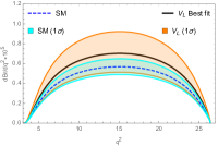
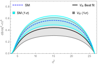
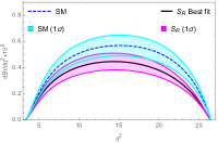
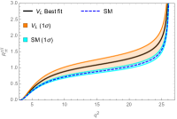
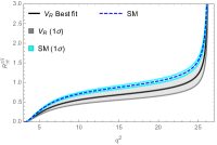
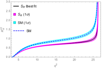
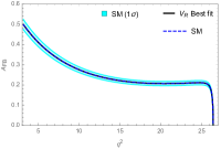
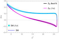
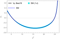
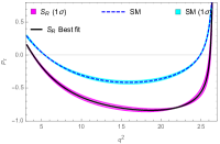
Figure 1: The $q^{2}$ (in ${\rm GeV}^{2}$) variation of differential branching fraction, lepton non-universaity parameter, forward-backward asymmetry and tau-polarization asymmetry of $\bar{B}^{0}\to\pi^{+}\tau^{-}\bar{\nu}$ process in the presence of additional $V_{L}$ coupling (left panel), $V_{R}$ coupling (middle panel) and $S_{R}$ coefficient (right panel).

Table 2: Branching fractions of $B\to(P,V)\mu^{-}\bar{\nu}_{\mu}$ in the Standard Model.

Decay Process	SM Branching ratio
$~{}{\rm Br}(\bar{B}^{0}\to\pi^{+}\mu^{-}\bar{\nu}_{\mu})$	$(1.533\pm 0.215)\times 10^{-4}$
${\rm Br}(\bar{B}^{0}\to\rho^{+}\mu^{-}\bar{\nu}_{\mu})$	$(4.024\pm 0.563)\times 10^{-4}$
${\rm Br}(B^{-}\to\omega\mu^{-}\bar{\nu}_{\mu})$	$(3.640\pm 0.510)\times 10^{-4}$
${\rm Br}(B_{s}\to K\mu^{-}\bar{\nu}_{\mu})$	$(0.950\pm 0.133)\times 10^{-4}$
${\rm Br}(B_{s}\to K^{*}\mu^{-}\bar{\nu}_{\mu})$	$(3.396\pm 0.475)\times 10^{-4}$

Table 3: Predicted values of branching fractions (in units of $10^{-4}$) and other observables for $B\to(P,V)\tau\bar{\nu}_{\tau}$ processes, both in the SM and NP scenarios.

Observables	SM prediction	with $V_{L}$ NP	with $V_{R}$ NP	with $S_{L}$ NP	with $S_{R}$ NP
${\rm Br}(\bar{B}^{0}\to\pi\tau\bar{\nu})$	$0.983\pm 0.138$	$0.886\to 1.596$	$0.534\to 1.066$	$0.808\to 1.116$	$0.649\to 0.857$
$R_{\pi}^{\tau/\ell}$	$0.641\pm 0.127$	$0.578\to 1.041$	$0.348\to 0.695$	$0.527\to 0.728$	$0.423\to 0.559$
$A_{\rm FB}$	$0.246\pm 0.012$	$0.234\to 0.258$	$0.234\to 0.258$	$0.237\to 0.245$	$0.045\to 0.067$
$P_{\tau}$	$-(0.298\pm 0.015)$	$-(0.313\to 0.283)$	$-(0.313\to 0.283)$	$-(0.360\to 0.304)$	$-(0.698\to 0.693)$
${\rm Br}(\bar{B}^{0}\to\rho\tau\bar{\nu})$	$2.142\pm 0.300$	$1.930\to 3.475$	$1.903\to 3.191$	$1.844\to 2.479$	$1.661\to 2.192$
$R_{\rho}^{\tau/\ell}$	$0.532\pm 0.105$	$0.480\to 0.864$	$0.473\to 0.793$	$0.458\to 0.616$	$0.413\to 0.545$
$A_{\rm FB}$	$-(0.178\pm 0.009)$	$-(0.187\to 169)$	$-(0.166\to 0.080)$	$-(0.177\to 0.168)$	$-(0.287\to 0.279)$
$P_{\tau}$	$-(0.544\pm 0.027)$	$-(0.571\to 0.517)$	$-(0.54\to 0.52)$	$-(0.542\to 0.521)$	$-(0.720\to 0.712)$
$F_{L}^{\rho}$	$0.502\pm 0.025$	$0.477\to 0.527$	$0.510\to 0.557$	$0.502\to 0.509$	$0.445\to 0.457$
${\rm Br}(B^{-}\to\omega\tau\bar{\nu})$	$1.948\pm 0.273$	$1.755\to 3.161$	$1.731\to 2.905$	$1.678\to 2.255$	$1.506\to 1.988$
$R_{\omega}^{\tau/\ell}$	$0.535\pm 0.106$	$0.482\to 0.868$	$0.475\to 0.798$	$0.461\to 0.619$	$0.414\to 0.546$
$A_{\rm FB}$	$-(0.119\pm 0.006)$	$-(0.125\to 0.113)$	$-(0.111\to 0.054)$	$-(0.119\to 0.112)$	$-(0.194\to 0.189)$
$P_{\tau}$	$-(0.538\pm 0.027)$	$-(0.565\to 0.511)$	$-(0.534\to 0.514)$	$-(0.537\to 0.515)$	$-(0.719\to 0.711)$
$F_{L}^{\omega}$	$(0.498\pm 0.025)$	$0.473\to 0.523$	$0.506\to 0.552$	$0.498\to 0.505$	$0.434\to 0.441$
${\rm Br}(B_{s}\to K\tau\bar{\nu})$	$0.729\pm 0.102$	$0.657\to 1.183$	$0.396\to 0.790$	$0.596\to 0.827$	$0.456\to 0.604$
$R_{K}^{\tau/\ell}$	$0.767\pm 0.152$	$0.692\to 1.245$	$0.417\to 0.832$	$0.627\to 0.870$	$0.48\to 0.636$
$A_{\rm FB}$	$(0.253\pm 0.013)$	$0.24\to 0.266$	$0.24\to 0.266$	$0.245\to 0.253$	$0.048\to 0.071$
$P_{\tau}$	$-(0.244\pm 0.012)$	$-(0.256\to 0.232)$	$-(0.256\to 0.232)$	$-(0.309\to 0.250)$	$-(0.713\to 0.710)$
${\rm Br}(B_{s}\to K^{*}\tau\bar{\nu})$	$1.817\pm 0.254$	$1.637\to 2.949$	$1.614\to 2.708$	$1.565\to 2.10$	$1.423\to 1.879$
$R_{K}^{\tau/\ell}$	$0.535\pm 0.106$	$0.482\to 0.868$	$0.475\to 0.797$	$0.461\to 0.618$	$0.419\to 0.553$
$A_{\rm FB}$	$-(0.130\pm 0.006)$	$-(0.136\to 0.124)$	$-(0.122\to 0.064)$	$-(0.130\to 0.124)$	$-(0.197\to 0.192)$
$P_{\tau}$	$-(0.565\pm 0.028)$	$-(0.593\to 0.537)$	$-(0.561\to 0.543)$	$-(0.563\to 0.544)$	$-(0.726\to 0.719)$
$F_{L}^{K^{*}}$	$(0.481\pm 0.024)$	$0.457\to 0.505$	$0.489\to 0.534$	$0.481\to 0.487$	$0.427\to 0.430$

Using these form factors, and the other input parameters e.g., the particle masses, lifetime of $B$ meson from Tanabashi et al. (2018), the branching fraction, $R_{\pi}^{\tau/\ell}$, forward-backward asymmetry and lepton polarization asymmetry parameters for $\bar{B}^{0}\to\pi^{+}\tau^{-}\bar{\nu}_{\tau}$ process are studied for various NP scenarios. The SM predicted branching ratio of $\bar{B}^{0}\to\pi^{+}\mu^{-}\bar{\nu}_{\mu}$ decay mode is presented in Table 2. The graphical representation of our results is displayed in Fig. 1, where we have shown the $q^{2}$ variation of various observables in different NP frameworks. The plots in the left panel (from top to bottom) represent the variation of differential branching fraction, LFU violating parameter, forward-backward asymmetry and the tau-polarization asymmetry respectively. In these plots, the blue-dashed lines correspond to SM result with central values of the input parameters, while the cyan band in the differential branching fraction plot is due to $1\sigma$ uncertainties in the form factor, CKM matrix element and other input parameters. The black solid lines depict the contribution from $V_{L}$ type NP (best-fit value), while the orange bands denote the corresponding $1\sigma$ uncertainties. Analogously, the results for $V_{R}$ type NP coupling are shown in the plots of the middle panel, while the plots in the right panel are for $S_{R}$ coupling and the colour-coding of these plots are provided in the plot legends. From the figures it should be noted that the branching fraction and the $R_{\pi}^{\tau/\ell}$ observable deviate substantially from their SM predictions. The interesting point to be noted from these plots is that, due to the NP contribution from $V_{L}$ type coupling, the values of these observables are enhanced with respect to their SM results, whereas they are reduced for $V_{R}$ and $S_{R}$ couplings. The forward-backward asymmetry and $P_{\tau}$ observables are insensitive to $V_{L}$ and $V_{R}$ couplings, while they differ considerably from their SM values for $S_{R}$ coupling. So we have not shown explicitly the $1\sigma$ uncertainties of these observables in the plots due to $V_{L}$ and $V_{R}$ couplings. Since these observables behave quite differently in various NP scenarios, their measurements will definitely shed light on the nature of the NP. Furthermore, as the effect of $S_{L}$ coupling is very nominal, the corresponding plots are not displayed explicitly. However, the integrated values of these observables in all four NP scenarios are presented in Table 3.

	$B\to\rho$	$B\to\omega$	$B_{s}\to K^{*}$
$a_{0}^{V}$	$0.33\pm 0.03$	$0.30\pm 0.04$	$0.30\pm 0.03$
$a_{1}^{V}$	$-0.86\pm 0.18$	$-0.83\pm 0.29$	$-0.90\pm 0.27$
$a_{2}^{V}$	$1.80\pm 0.97$	$1.72\pm 1.24$	$2.65\pm 1.33$
$a_{0}^{A_{0}}$	$0.36\pm 0.04$	$0.33\pm 0.05$	$0.31\pm 0.05$
$a_{1}^{A_{0}}$	$-0.83\pm 0.20$	$-0.83\pm 0.30$	$-0.66\pm 0.23$
$a_{2}^{A_{0}}$	$1.33\pm 1.05$	$1.42\pm 1.25$	$2.57\pm 1.44$
$a_{0}^{A_{1}}$	$0.26\pm 0.03$	$0.24\pm 0.03$	$0.23\pm 0.03$
$a_{1}^{A_{1}}$	$0.39\pm 0.14$	$0.34\pm 0.24$	$0.27\pm 0.19$
$a_{2}^{A_{1}}$	$0.16\pm 0.41$	$0.09\pm 0.57$	$0.13\pm 0.56$
$a_{0}^{A_{12}}$	$0.30\pm 0.03$	$0.27\pm 0.04$	$0.23\pm 0.03$
$a_{1}^{A_{12}}$	$0.76\pm 0.20$	$0.66\pm 0.26$	$0.60\pm 0.21$
$a_{2}^{A_{12}}$	$0.46\pm 0.76$	$0.28\pm 0.98$	$0.54\pm 1.12$

Table 4: Values of the various expansion coefficients ($a_{k}^{i}$) for $B\to\rho$, $B\to\omega$ and $B_{s}\to K^{*}$ processes.

IV.2 $B\to(\rho,\omega)\tau\bar{\nu}$ decay

The matrix elements of the vector and scalar currents associated with $\bar{B}\to V\ell\bar{\nu}_{\ell}$ decay process can be expressed as,

$$\langle V(k,\varepsilon)|\bar{u}\gamma_{\mu}b|\bar{B}|(p_{B})\rangle=-i\epsilon_{\mu\nu\alpha\beta}\varepsilon^{\nu*}p_{B}^{\alpha}k^{\beta}\frac{2V(q^{2})}{m_{B}+m_{V}},$$

$$\langle V(k,\varepsilon)|\bar{u}\gamma_{\mu}\gamma_{5}b|\bar{B}|(p_{B})\rangle=\varepsilon_{\mu}^{*}(m_{B}+m_{V})A_{1}(q^{2})-(p_{B}+k)_{\mu}(\varepsilon^{*}\cdot q)\frac{A_{2}(q^{2})}{m_{B}+m_{V}}$$

$$~{}~{}~{}~{}~{}~{}~{}~{}~{}~{}~{}~{}~{}~{}~{}~{}~{}\quad\quad~{}~{}~{}~{}~{}~{}~{}~{}~{}~{}~{}-q_{\mu}(\varepsilon^{*}\cdot q)\frac{2m_{V}}{q^{2}}\left[A_{3}(q^{2})-A_{0}(q^{2})\right],$$

$$\langle V(k,\varepsilon)|\bar{u}\gamma_{5}b|\bar{B}|(p_{B})\rangle=-\frac{1}{m_{b}+m_{u}}q_{\mu}\langle V(k,\epsilon)|\bar{u}\gamma^{\mu}\gamma^{5}b|\bar{B}|(p_{B})\rangle$$

$$~{}~{}~{}~{}~{}~{}~{}~{}~{}~{}~{}~{}~{}~{}~{}~{}~{}~{}~{}~{}~{}~{}~{}~{}~{}~{}~{}~{}~{}=-(\varepsilon^{*}\cdot q)\frac{2m_{V}}{m_{b}+m_{u}}A_{0}(q^{2}).$$ (18)

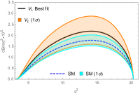
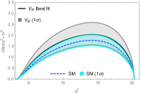
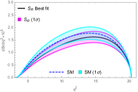
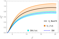
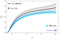
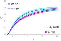
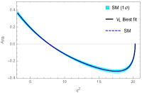
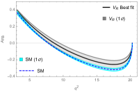
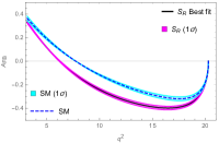
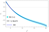
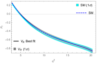
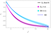
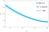
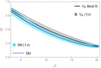
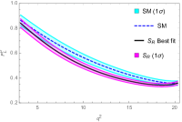
Figure 2: The $q^{2}$ (in ${\rm GeV}^{2}$) variation of different observables of $\bar{B}^{0}\to\rho\tau^{-}\bar{\nu}_{\tau}$ in the presence of new $V_{L}$ coupling (left panel), $V_{R}$ coupling (middle panel) and $S_{R}$ coupling (right panel).

The $q^{2}$ dependence of the form factors are determined by performing a combined fit to lattice and LCSR results, which are valid for the entire kinematic range Bharucha et al. (2016), and are parametrized as

$$F_{i}(q^{2})=\frac{1}{(1-q^{2}/m_{R,i}^{2})}~{}\sum_{k=0}a_{k}^{i}\Big{[}z(q^{2})-z(0)\Big{]}^{k},$$ (19)

where $z(q^{2})=\frac{\sqrt{t_{+}-q^{2}}-\sqrt{t_{+}-t_{0}}}{\sqrt{t_{+}-q^{2}}+\sqrt{t_{+}+t_{0}}}$ with $t_{\pm}=(m_{B}\pm m_{V})^{2}$ and $t_{0}=t_{+}(1-\sqrt{1-t_{-}/t_{+}})$. The form-factor $F_{i}$ refers to $V(q^{2})$, $A_{0}(q^{2})$, $A_{1}(q^{2})$ and $A_{12}(q^{2})$, where $A_{12}(q^{2})$ is defined as

$$A_{12}(q^{2})=\frac{(m_{B}+m_{V})^{2}(m_{B}^{2}-m_{V}^{2}-q^{2})A_{1}(q^{2})-\lambda_{V}(q^{2})A_{2}(q^{2})}{16m_{B}m_{V}^{2}(m_{B}+m_{V})}.$$ (20)

The values of the different $a_{k}^{i}$ coefficients used in our analysis are presented in Table 4. Using these values and other input parameters from Tanabashi et al. (2018), we estimate the branching fraction, $R^{\tau/\ell}_{\rho}$, $A_{FB}$, $P_{\tau}$ and $F_{L}^{\rho}$ observables for $\bar{B}^{0}\to\rho\tau^{-}\bar{\nu}_{\tau}$ process in the presence of the NP coefficients $V_{L}$, $V_{R}$, $S_{L}$ and $S_{R}$, and the $q^{2}$ variation of these observables are displayed in Fig 2. Since there is almost negligible deviation of these observables from their SM prediction in the presence of $S_{L}$ coefficient, the corresponding results are not shown in the figure. It can be noticed from the figure that the branching fraction and the LFU violating observable have significant deviation from their SM results in the presence of $V_{L}$, $V_{R}$ and $S_{R}$ NP scenarios, whereas only $V_{R}$ and $S_{R}$ NP contributions can affect $A_{\rm FB}$, $P_{\tau}$ and $F_{L}^{\rho}$ observables. The estimated average values of these observables are presented in Tab. 3 and the branching fraction of $\bar{B}^{0}\to\rho^{-}\mu^{+}\nu_{\mu}$ is furnished in Table 2.

Similarly for $B^{-}\to\omega\tau^{-}\bar{\nu}_{\tau}$ process, use the form factors from Bharucha et al. (2016), we calculate the values of various observables. Since the $q^{2}$ dependence of these observables have almost the similar behaviour as $B^{0}\to\rho\tau^{-}\bar{\nu}_{\tau}$ process, we do not provide the graphical results, however, their numerical results are presented in Table 3. In this case also the branching fraction deviates significantly from the SM prediction with $V_{L}$, $V_{R}$ and $S_{R}$ type of new physics. Furthermore, $V_{R}$ and $S_{R}$ kind of new physics affect marginally the forward backward asymmetry and the longitudinal polarization of $\omega$ meson.

IV.3 $B_{s}\to(K,K^{*})\tau\bar{\nu}$ decay

We use the form factors for $B_{s}\to K\ell\bar{\nu}$ transition from lattice QCD calculation Bazavov et al. (2019), with the BCL parametrization

$$f_{+}(q^{2})=\frac{1}{(1-q^{2}/m_{B^{*}(1^{-})})}\sum_{n=1}^{N-1}b_{n}^{+}(t_{0})\Big{[}z^{n}-(-1)^{n-N}\frac{n}{N}z^{N}\Big{]}$$

$$f_{0}(q^{2})=\frac{1}{(1-q^{2}/m_{B^{*}(0^{+}))}}\sum_{n=1}^{N-1}b_{n}^{0}(t_{0})~{}z^{n},$$ (21)

where the factor $1/(1-q^{2}/m_{B^{*}}^{2})$ take the poles into account and ensure the asymptotic scaling. The expansion parameter $z$ is defined as

$$z(q^{2},t_{0})=\frac{\sqrt{t_{\rm cut}-q^{2}}-\sqrt{t_{\rm cut}-t_{0}}}{\sqrt{t_{\rm cut}-q^{2}}+\sqrt{t_{\rm cut}-t_{0}}}$$ (22)

where $t_{\rm cut}$ is the particle pair production threshold with value ${\sqrt{t}_{\rm cut}}=5.414$ GeV and $t_{0}=t_{\rm cut}-\sqrt{t_{\rm cut}(t_{\rm cut}-t_{-})}$ with $t_{-}=(m_{B_{s}}-m_{K})^{2}$. The values of the pole masses are $m_{B^{*}}(1^{-})=5.325$ GeV and $m_{B^{*}}(0^{+})=5.68$ GeV, and the expansion parameters have values Bazavov et al. (2019)

$$b^{+}_{0}=0.3623(0.0178),\quad b^{+}_{1}=-0.9559(0.1307),\quad b^{+}_{2}=-0.8525(0.4783),$$

$$b^{+}_{3}=0.2785(0.6892),\quad b^{0}_{0}=0.1981(0.0101),\quad b^{0}_{1}=-0.1661(0.1130),$$

$$b^{0}_{2}=-0.6430(0.4385),\quad b^{0}_{3}=-0.3754(0.4535).$$ (23)

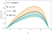
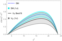
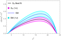
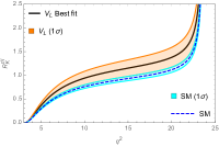
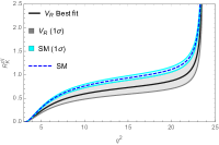
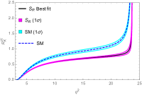
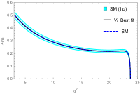
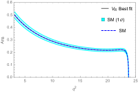
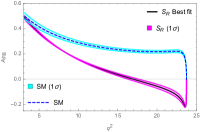
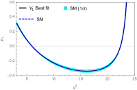
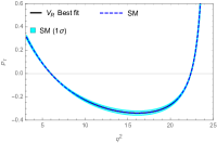
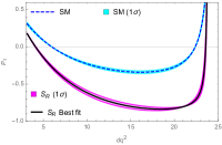
Figure 3: The $q^{2}$ (in ${\rm GeV}^{2}$) variation of branching fraction, $R_{K}^{\tau/\ell}$, $A_{\rm FB}$, $P_{\tau}$ observables for $B_{s}\to K\tau\bar{\nu}_{\tau}$ process in the presence of $V_{L}$, $V_{R}$ and $S_{R}$ NP scenarios.

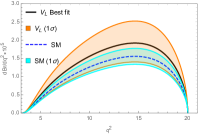
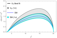
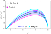
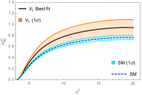
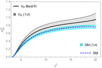
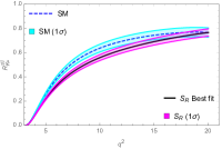
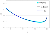
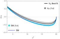
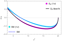
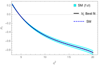
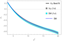
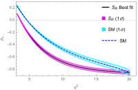
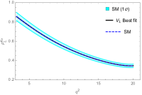
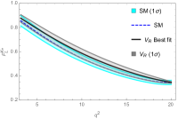
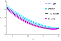
Figure 4: Same as Figure 2, for $B_{s}\to K^{*}\tau\bar{\nu}_{\tau}$ process.

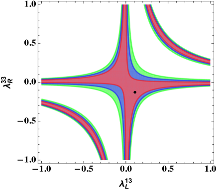
Figure 5: Constraints on LQ parameter space from the current experimental data on ${\rm Br}(B_{u}\to\tau\bar{\nu}_{\tau})$, ${\rm Br}(B\to\pi\tau\bar{\nu}_{\tau})$ and $R_{\pi}^{\ell}$. Different colors represent the $1\sigma$, $2\sigma$ and $3\sigma$ contours and the black dot represents the best-fit value.

With these values of the form factors, we show the $q^{2}$ variation of branching fraction, lepton non-universality parameter, forward-backward asymmetry, and tau polarization asymmetry in Fig. 3. From the figure, it can be seen that the branching fraction and the LNU parameter deviate significantly from their SM values in the presence of $V_{L}$, $V_{R}$ and $S_{R}$ NP scenarios. However, due to the effect of $V_{L}$, the branching ratio is enhanced with respect to its SM value, whereas its value is found to be lower than the SM prediction in the presence of $V_{R}$ and $S_{R}$. Furthermore, though the forward-backward asymmetry remain unaffected due to the $V_{L}$ and $V_{R}$ contribution, the impact of $S_{R}$ is found to be quite substantial. Thus, the measurement of these observables will help to discriminate various kinds of NP scenarios. The numerical values of these observables are presented in Table 3.

For $B_{s}\to K^{*}\tau\nu$, the values of the form factors (18,19) are taken from Bharucha et al. (2016), and the corresponding expansion coefficients are provided in Table 4. With these values, the $q^{2}$ dependence of the various observables is shown in Fig. 4. In this case also, the branching fraction and the LNU parameters have substantial deviations from their SM values in the upward direction for $V_{L,R}$ and in downward direction for $S_{R}$. The $P_{\tau}$ and $F_{L}^{K^{*}}$ observables show only marginal deviation for $V_{R}$ and $S_{R}$ scenarios. The numerical values of these observables are presented in Table 3.

V Leptoquark: An example of New Physics scenario

In this section, we will discuss the effect of leptoquarks on $b\to u\tau\nu$ transitions as a possible new physics scenario. We will consider two possible leptoquark models: the scalar leptoquark $R_{2}(3,2,7/6)$ and the vector leptoquark $U_{1}(3,1,2/3)$, which are found to be quite successful in addressing the recent flavour anomalies associated with $b\to c\ell\bar{\nu}_{\ell}$ transition.

V.1 Comment on effect of scalar leptoquark $R_{2}(3,2,7/6)$

Here we consider the example of scalar leptoquark (LQ) $R_{2}(3,2,7/6)$ as the NP scenario, where the quantum numbers in the parenthesis represent its values under the SM gauge group $SU(3)_{C}\times SU(2)_{L}\times U(1)_{Y}$ and briefly discuss its implication on various observables of $b\to u\tau\bar{\nu}$ transition. The $SU(2)_{L}$ doublet scalar LQ can generate significant contribution to $b\to c\ell\bar{\nu}$ processes and can explain the observed experimental data quite well Sakaki et al. (2013); Iguro et al. (2019). Additionally, it also safeguards the proton decay, as the diquark coupling is absent. It couples to quark and lepton fields flavour dependently via Yukawa couplings and the interaction Lagrangian involving $R_{2}$ can be expressed as

$${\cal L}_{\rm int}=\lambda_{R}^{ij}\bar{Q}_{Li}\ell_{Rj}R_{2}-\lambda_{L}^{ij}\bar{u}_{Ri}R_{2}i\tau_{2}L_{Lj}+{\rm h.c.},$$ (24)

where $\lambda_{L,R}$ are the $3\times 3$ complex matrices, $Q_{L}(L_{L})$ is the left-handed quark (lepton) doublets, $u_{R}(\ell_{R})$ is the right-handed up-type quark (charged lepton) singlet and $i,j$ are the generation indices. After expansion of the $SU(2)$ indices, the interaction Lagrangian (24) in the mass basis can be expressed as

$${\cal L}_{\rm int} = (V_{\rm CKM}\lambda_{R})^{ij}\bar{u}_{Li}\ell_{Rj}R_{2}^{(5/3)}+\lambda_{R}^{ij}\bar{d}_{Li}\ell_{Rj}R_{2}^{(2/3)}$$ (25)

$$+ \lambda_{L}^{ij}\bar{u}_{Ri}\nu_{Lj}R_{2}^{(2/3)}-\lambda_{L}^{ij}\bar{u}_{Ri}\ell_{Lj}R_{2}^{(5/3)}+{\rm h.c.},$$

where the superscripts in $R_{2}$ denote its electric charge and we consider the mass basis for quark doublet fields as $((V_{\rm CKM}^{\dagger}u_{L})^{i},d_{L}^{i})^{T}$ and lepton fields as $(\nu_{L}^{i},\ell_{L}^{i})^{T}$, ignoring the mixing in the lepton sector, i.e., the lepton mixing matrix is assumed to be unit matrix. Thus, it can be noted from (25) that the exchange of $R_{2}^{(2/3)}$ can give rise to new contribution to $b\to u\tau\bar{\nu}_{\tau}$ transition at tree-level and generate the scalar and tensor operators at the LQ mass scale $(\mu_{\rm LQ})$ as:

$${S_{L}}(\mu_{\rm LQ})=4{T_{L}}(\mu_{\rm LQ})=\frac{1}{4\sqrt{2}G_{F}V_{ub}}\frac{\lambda_{L}^{13}(\lambda_{R}^{33})^{*}}{m_{\rm LQ}^{2}}\;,$$ (26)

where $m_{\rm LQ}$ is the mass of the leptoquark, and we consider a typical representative value for LQ mass as 1 TeV, in this analysis. The new coefficients in (26) depend on the NP scale $(\mu(m_{\rm LQ}))$, and it is imperative to consider the renormalization-group (RG) equation to evolve their values from NP scale to effective Hamiltonian matching scale $\mu=m_{b}$, and are related as Gonzalez-Alonso et al. (2017); Blanke et al. (2019)

$$\begin{pmatrix}{S_{L}}(m_{b})\\ {T_{L}}(m_{b})\end{pmatrix}=\begin{pmatrix}1.752&-0.287\\ -0.004&0.842\end{pmatrix}\begin{pmatrix}{S_{L}}(1~{}{\rm TeV})\\ {T_{L}}(1~{}{\rm TeV})\end{pmatrix}.$$ (27)

Performing a $chi$-square fit to the current experimental data on ${\rm Br}(B_{u}\to\tau\bar{\nu}_{\tau})$, ${\rm Br}(B\to\pi\tau\bar{\nu}_{\tau})$ and $R_{\pi}^{\ell}$, and assuming the LQ couplings to be real, the best-fit values for the couplings are found to be $(\lambda_{L}^{13},\lambda_{R}^{33})=(0.110,-0.129)$ and the corresponding allowed parameter space is shown in Fig. 5, where different colors represent the contours for $1\sigma$, $2\sigma$ and $3\sigma$ allowed regions. Translating the obtained values of LQ coupling to the new scalar coupling through (26) and (27), we obtain

$${S_{L}}=-0.033,$$ (28)

which is basically same order as the obtained value following model-independent approach. Therefore, one can conclude that the effect of the scalar LQ $R_{2}$ on various observables of $b\to u\tau\bar{\nu}$ is quite minimal and hence, we do not provide their explicit values again for this scenario.

V.2 Comment on effect of scalar leptoquark $U_{1}(3,1,2/3)$

The vector leptoquark $U_{1}(3,1,2/3)$ has received a lot of attention in recent times as it provides a simultaneous explanation to the observed flavour anomalies associated with $b\to c\ell\bar{\nu}_{\ell}$ and $b\to s\ell^{+}\ell^{-}$ transitions. The interaction Lagrangian describing the interaction between the $U_{1}$ LQ and the SM fermions can be represented as

$${\cal L}=\lambda_{L}^{ij}\overline{Q}_{i}\gamma_{\mu}U_{1}^{\mu}L_{j}+\lambda_{R}^{ij}\overline{d}_{Ri}\gamma_{\mu}U_{1}^{\mu}\ell_{Rj}+{\rm h.c.},$$ (29)

where $\lambda_{L,R}^{ij}$ are the $3\times 3$ complex matrices. After integrating out the heavy vector leptoquark $U_{1}$, the new Wilson coefficients contributing to $b\to u\tau\bar{\nu}_{\tau}$ are expressed as

$${V_{L}}(\mu_{\rm LQ})=\frac{(V_{\rm CKM}\lambda_{L})^{13}(\lambda_{L}^{33})^{*}}{2\sqrt{2}G_{F}V_{ub}~{}m_{U_{1}}^{2}}$$

$${S_{R}}(\mu_{\rm LQ})=-\frac{(V_{\rm CKM}\lambda_{L})^{13}(\lambda_{R}^{33})^{*}}{\sqrt{2}G_{F}V_{ub}~{}m_{U_{1}}^{2}}.$$ (30)

For simplicity, we consider only the diagonal CKM matrix element $V_{11}$ to reduce the number of LQ couplings. We further assume these couplings to be real. The values of these coefficients at the $m_{b}$ scale is obtained using the renormalization group equation Gonzalez-Alonso et al. (2017); Blanke et al. (2019)

$$V_{L}(m_{b})=V_{L}(1~{}{\rm TeV}),~{}~{}~{}~{}~{}S_{R}(m_{b})=1.737S_{R}(1~{}{\rm TeV}).$$ (31)

Since, there are three new couplings, i.e., $\lambda_{L}^{13}$, $\lambda_{L}^{33}$, $\lambda_{R}^{33}$, it would be challenging to constrain them with three observables ${\rm Br}(B_{u}\to\tau\bar{\nu}_{\tau})$, ${\rm Br}(B\to\pi\tau\bar{\nu}_{\tau})$ and $R_{\pi}^{\ell}$, we therefore assume that either ${V_{L}}$ or ${S_{R}}$ coupling will present at a given instant, (i.e., the presence of only two real couplings at a given time). Now considering the presence of $\lambda_{L}^{13}$ and $\lambda_{R}^{33}$, the bounds on the LQ couplings are obtained by performing a $\chi^{2}$ fit, with the best-fit values obtained as $(\lambda_{L}^{13},\lambda_{R}^{33})=(0.064,-0.057)$ and the allowed parameter space in the $\lambda_{L}^{13}-\lambda_{R}^{33}$ plane is shown in the left panel of Fig. 6, where different colors correspond to 1, 2, and 3$\sigma$ regions respectively and the black point represents the best-fit value. Similarly, considering $\lambda_{L}^{13}$ and $\lambda_{L}^{33}$ couplings, the best-fit values obtained are $(\lambda_{L}^{13},\lambda_{L}^{33})=(0.121,0.1155)$ and the corresponding allowed parameter space is shown in the right panel of Fig. 6. With Eqns (30) and 31), these best-fit results give the values of the new couplings as

$${S_{R}}=0.033,~{}~{}~{}~{}~{}{\rm and}~{}~{}~{}~{}~{}{V_{L}}=0.11.$$ (32)

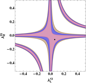
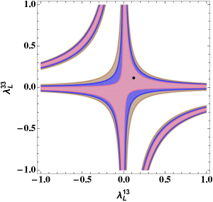
Figure 6: Allowed parameter space for $U_{1}$ Leptoquark couplings in $\lambda^{13}_{L}-\lambda_{R}^{33}$ plane (left panel) and $\lambda^{13}_{L}-\lambda_{L}^{33}$ plane (right-panel), where pink, blue and brown colors show the one, two and three-sigma allowed regions and the black points represent the best-fit values.

As, the value of the scalar coupling ${S_{R}}$ is negligibly small, we show the effect of $U_{1}$ leptoquark with two non-zero real couplings, i.e., due to ${V_{L}}$, on the branching fraction and the LNU observable for the process $B\to\pi\tau\bar{\nu}~{}(B\to\rho\tau\bar{\nu})$ in he left (right) panel of Fig. 7. From the Figure, it can be seen that these observables deviate significantly from their SM predictions due the effect of $U_{1}$ leptoquark. Other observables like forward-backward asymmetry and polarization asymmetries do not get affected by the new vector coupling and will remain consistent with their corresponding SM values. The integrated values of these observables for various processes are provided in Table 5.

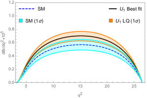
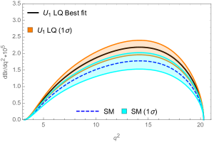
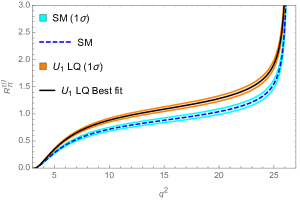
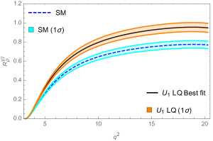
Figure 7: The $q^{2}$ variation of branching fraction and the LNU observable for the $\bar{B}^{0}\to\pi^{+}\tau\bar{\nu}_{\tau}$ $(\bar{B}^{0}\to\rho^{+}\tau\bar{\nu}_{\tau})$ process shown in the left (right) panel.

Table 5: Predicted values of branching fractions (in units of $10^{-4}$) and LNU observables $R_{P,V}^{\tau/\ell}$ for $B\to(P,V)\tau\bar{\nu}_{\tau}$ processes in $U_{1}$ LQ model.

Decay process	Branching fraction	$R^{\tau/\ell}$
$B\to\pi\tau\bar{\nu}$	$(1.21\pm 0.12)$	$0.789\pm 0.136$
$B\to\rho\tau\bar{\nu}$	$(2.64\pm 0.26)$	$0.656\pm 0.112$
$B\to\omega\tau\bar{\nu}$	$(2.40\pm 0.24)$	$0.659\pm 0.113$
$B_{s}\to K\tau\bar{\nu}$	$(0.90\pm 0.09)$	$0.947\pm 0.163$
$B_{s}\to K^{*}\tau\bar{\nu}$	$(2.24\pm 0.22)$	$0.660\pm 0.113$

VI Conclusion

It is well-known that the Standard Model gauge interactions strictly respect lepton flavour universality and any violation of it would point towards the possible role of new physics. The recent observation of several LFU violating signals in the charged current transitions $b\to c\ell\bar{\nu}_{\ell}$ in the form of $R_{D}$, $R_{D^{*}}$ and $R_{J/\psi}$ created huge excitement in the flavour physics community. To account for these discrepancies, it is generally assumed the attribution of new physics to the semitauonic process $b\to c\tau\bar{\nu}_{\tau}$. Thus, if indeed new physics is present in this decay process, its footprint can also be seen in the allied charged-current process $b\to u\tau\bar{\nu}_{\tau}$, as these two processes have the same topologies, apart from the fact that the latter process is Cabibbo suppressed. Therefore, in this article, we have performed a model independent analysis of semileptonic processes mediated through $b\to u\tau\bar{\nu}$ transition in the presence of new physics. In particular, we focus on the decay modes $B^{0}\to\pi^{+}\tau^{-}\bar{\nu}_{\tau}$, $B\to(\rho,\omega)\tau\bar{\nu}_{\tau}$ and $B_{s}\to(K,K^{*})\tau\bar{\nu}_{\tau}$. The new physics couplings are constrained by using experimental data on the branching fractions of $B_{u}\to\tau\bar{\nu}_{\tau}$, $B\to\pi\tau\bar{\nu}_{\tau}$ and $R_{\pi}^{\ell}$. Using the best-fit values and the corresponding $1\sigma$ ranges of NP couplings, we show the $q^{2}$ variation of different observables and their sensitivity towards new physics. In particular, we have estimated the values of branching fractions, lepton non-universality parameters, forward-backward asymmetry, $\tau$ polarization asymmetry and the longitudinal polarization of the final vector meson in the presence of individual new coupling. The differential branching fractions of all the processes showed a spectacular deviation from their SM predictions in the presence of $V_{L},V_{R}$ and $S_{R}$ couplings whereas no deviation is found in the presence of $S_{L}$ coefficient. However, the nature of deviation in ${\rm Br}(B\to V\tau\bar{\nu})$ transitions for $V_{L}$ type NP is opposite to those of $V_{R}$ and $S_{R}$ couplings. We also noticed appreciable deviation in the LNU parameters in the presence of the $V_{L}$, $V_{R}$ and $S_{R}$ coefficients. Lepton spin asymmetry parameters almost consistent with their SM values for $V_{L},V_{R}$ and $S_{L}$ couplings, but in the presence of $S_{R}$ coupling they deviate considerably from their SM values. $S_{L}$ coefficient remains almost insensitive for all the observables. These observed features can help us to discriminate between different NP scenarios and to reveal the true nature of NP, if at all its presence is affirmed. We also investigated the leptoquark model as an example and considered two specific scenarios: the $R_{2}(3,2,7/6)$ scalar leptoquark and $U_{1}(3,1,2/3)$ vector leptoquark. Assuming the coupling between the leptoquark and the SM fermions to be real, it has been found that the effect of $R_{2}(3,2,7/6)$ scalar leptoquark is negligible while the vector leptoquark $U_{1}(3,1,2/3)$ can significantly enhance the values of branching fractions and LNU observables. Concerning the future prospects of these decay modes, they have great potential to be observed in the LHCb and Belle-II experiments and thus observation of these modes will definitely shed light on the interplay of new physics on $b\to u\tau\bar{\nu}_{\tau}$ transition. In addition, the search for lepton nonuniversality observables $R_{P,V}^{\tau/\ell}$ is very promising as they also have significant deviation from their SM values for all these decay processes. Hence, observation of these observables can be used as an ideal probe to either confirm or rule out the presence of new physics. To conclude, these decay processes offer an alternative probe to study the implications of NP associated with the current $B$ anomalies in semileptonic transitions and could be accessible with the currently running LHCb and Belle II experiments.

Appendix: Helicity dependent differential decay rate

The $q^{2}$ distribution of the $B\to P\tau\bar{\nu}$ decay rates for a given $\tau$ polarization are given as

$$\frac{d\Gamma(\lambda_{\tau}=1/2)}{dq^{2}} = \frac{G_{F}^{2}|V_{ub}|^{2}}{192\pi^{3}m_{B}^{3}}q^{2}\sqrt{\lambda_{P}(q^{2})}\left(1-\frac{m_{\tau}^{2}}{q^{2}}\right)^{2}\Big{\{}\frac{1}{2}|1+V_{L}+V_{R}|^{2}\frac{m_{\tau}^{2}}{q^{2}}(H_{V,0}^{s~{}2}+3H_{V,t}^{s~{}2}$$ (33)

$$+ \frac{3}{2}|S_{R}+S_{L}|^{2}H_{S}^{s~{}2}+8|T_{L}|^{2}H_{T}^{s~{}2}-4{\rm Re}[(1+V_{L}+V_{R})T_{L}^{*}]\frac{m_{\tau}}{\sqrt{q^{2}}}H_{T}^{s}H_{V,0}^{s}$$

$$+ 3{\rm Re}[(1+V_{L}+V_{R})(S_{R}^{*}+S_{L}^{*})]\frac{m_{\tau}}{\sqrt{q^{2}}}H_{S}^{s}H_{V,t}^{s}\Big{\}},$$

$$\frac{d\Gamma(\lambda_{\tau}=-1/2)}{dq^{2}} = \frac{G_{F}^{2}|V_{ub}|^{2}}{192\pi^{3}m_{B}^{3}}q^{2}\sqrt{\lambda_{P}(q^{2})}\left(1-\frac{m_{\tau}^{2}}{q^{2}}\right)^{2}\Big{\{}|1+V_{L}+V_{R}|^{2}H_{V,0}^{s~{}2}+16|T_{L}|^{2}\frac{m_{\tau}^{2}}{q^{2}}H_{T}^{s~{}2}$$ (34)

$$- 8{\rm Re}[(1+V_{L}+V_{R})T_{L}^{*}]\frac{m_{\tau}}{\sqrt{q^{2}}}H_{T}^{s}H_{V,0}^{s}\Big{\}}.$$

Helicity dependent differential decay rate for $B\to V\tau\bar{\nu}$ process can be expressed as,

$$\frac{d\Gamma(\lambda_{\tau}=\frac{1}{2})}{dq^{2}} = \frac{G_{F}^{2}|V_{ub}|^{2}}{192\pi^{3}m_{\bar{B}}^{3}}q^{2}\sqrt{\lambda_{V}(q^{2})}\left(1-{m_{\tau}^{2}\over q^{2}}\right)^{2}$$ (36)

$$\times \Big{\{}\frac{1}{2}(|1+V_{L}|^{2}+|V_{R}|^{2}){m_{\tau}^{2}\over q^{2}}(H_{V,+}^{2}+H_{V,-}^{2}+H_{V,0}^{2}+3H_{V,t}^{2})$$

$$-{\rm Re}[(1+V_{L})V_{R}^{*}]{m_{\tau}^{2}\over q^{2}}(H_{V,0}^{2}+2H_{V,+}H_{V,-}+3H_{V,t}^{2})+{3\over 2}|S_{R}-S_{L}|^{2}H_{S}^{2}$$

$$+8|T_{L}|^{2}(H_{T,+}^{2}+H_{T,-}^{2}+H_{T,0}^{2})+3{\rm Re}[(1+V_{L}-V_{R})(S_{R}^{*}-S_{L}^{*})]\frac{m_{\tau}^{2}}{\sqrt{q^{2}}}H_{S}H_{V,t}$$

$$-4{\rm Re}[(1+V_{L})T_{L}^{*}]\frac{m_{\tau}}{\sqrt{q^{2}}}(H_{T,0}H_{V,0}+H_{T,+}H_{V,+}-H_{T,-}H_{V,-})$$

$$+4{\rm Re}[V_{R}T_{L}^{*}]\frac{m_{\tau}}{\sqrt{q^{2}}}(H_{T,0}H_{V,0}+H_{T,+}H_{V,-}-H_{T,-}H_{V,+})\Big{\}},$$

$$\frac{d\Gamma(\lambda_{\tau}=-\frac{1}{2})}{dq^{2}} = \frac{G_{F}^{2}|V_{ub}|^{2}}{192\pi^{3}m_{\bar{B}}^{3}}q^{2}\sqrt{\lambda_{V}(q^{2})}\left(1-\frac{m_{\tau}^{2}}{q^{2}}\right)^{2}\Big{\{}(|1+V_{L}|^{2}+|V_{R}|^{2})(H_{V,+}^{2}+H_{V,-}^{2}+H_{V,0}^{2})$$ (37)

$$-2{\rm Re}[(1+V_{L})V_{R}^{*}](H_{V,0}^{2}+2H_{V,+}H_{V,-})+16|T_{L}|^{2}\frac{m_{\tau}^{2}}{q^{2}}(H_{T,+}^{2}+H_{T,-}^{2}+H_{T,0}^{2})$$

$$-8{\rm Re}[(1+V_{L})T_{L}^{*}]\frac{m_{\tau}}{\sqrt{q^{2}}}(H_{T,0}H_{V,0}+H_{T,+}H_{V,+}-H_{T,-}H_{V,-})$$

$$+8{\rm Re}[V_{R}T_{L}^{*}]\frac{m_{\tau}}{\sqrt{q^{2}}}(H_{T,0}H_{V,0}+H_{T,+}H_{V,-}-H_{T,-}H_{V,+})\Big{\}}.$$

The decay distribution for the longitudinal polarization of final $V$ meson is given as

$$\frac{d\Gamma(\lambda_{V}=0)}{dq^{2}} = \frac{G_{F}^{2}|V_{ub}|^{2}}{192\pi^{3}m_{B}^{3}}q^{2}\sqrt{\lambda_{V}(q^{2})}\left(1-\frac{m_{\tau}^{2}}{q^{2}}\right)^{2}\Big{\{}|1+V_{L}-V_{R}|^{2}\left[\left(1+\frac{m_{\tau}^{2}}{2q^{2}}\right)H_{V,0}^{2}+\frac{3}{2}\frac{m_{\tau}^{2}}{q^{2}}H_{V,t}^{2}\right]$$ (38)

$$+ \frac{3}{2}|S_{R}-S_{L}|^{2}H_{S}^{2}+8|T_{L}|^{2}\left(1+\frac{2m_{\tau}^{2}}{q^{2}}\right)H_{T,0}^{2}-12{\rm Re}[(1+V_{L}-V_{R})T_{L}^{*}]\frac{m_{\tau}}{\sqrt{q^{2}}}H_{T,0}H_{V,0}$$

$$+ 3{\rm Re}[(1+V_{L}-V_{R})(S_{R}^{*}-S_{L}^{*})]\frac{m_{\tau}}{\sqrt{q^{2}}}H_{S}H_{V,t}\Big{\}}.$$