Thermal Operations in general are not memoryless

Abstract

So-called Thermal Operations seem to describe the most fundamental, and reasonable, set of operations allowable for state transformations at an ambient inverse temperature $\beta$. However, a priori, they require experimentalists to manipulate very complex environments and have control over their internal degrees of freedom. For this reason, the community has been working on creating more experimentally-friendly operations. In [Perry et al., Phys. Rev. X 8, 041049] it was shown that for states diagonal in the energy basis, that Thermal Operations can be performed by so-called Coarse Operations, which need just one auxiliary qubit, but are otherwise Markovian and classical in spirit. In this work, by providing an explicit counterexample, we show that this one qubit of memory is necessary. We also fully characterize the possible transitions that do not require memory for the system being a qubit. We do this by analyzing arbitrary control sequences comprising level energy changes and partial thermalizations in each step.

I Introduction

Due to the rapid growth of technology, the field of quantum thermodynamics is booming. The advent of nanotechnology has risen a plethora of questions about quantum and discrete-size effects in thermodynamics. Already in the past couple of years, we can observe experimental progress in studying thermodynamics at the quantum level [1, 2, 3, 4]. One of the fundamental questions in this field is which states can be converted into one another via a suitable set of operations. Of course, defining the suitable set of operations is no easy task, and much work has been devoted into solving this question. Of particular interest, is the set of Thermal Operations [5, 6, 7, 8] which have been recently widely used within a resource-theoretic approach to quantum thermodynamics [9, 10]. In a nutshell, Thermal Operations consist of appending a heat bath to the system, applying energy conserving unitary transformation, and then discarding the heat bath.

It is not known in general, whether a given state can be transformed into another state by Thermal Operations [11, 12]. Yet for states diagonal in the energy basis, the transformation $\rho\xrightarrow{\text{TO}}\sigma$ is allowed iff $\rho$ “thermomajorizes” $\sigma$, i.e., $\rho\succ_{T}\sigma$ [8, 13]. This “thermomajorization” condition can also be used to calculate how much deterministic work can be extracted from a state, by appending a 2-level battery (work bit) and maximizing over the energy gap of the battery. The problem with Thermal Operations, however, is that as used in [8], they are intractable for experiments. The energy-conserving unitary $U$ would have to be very delicately made, and couple the system to the bath in extremely precise ways. Furthermore, the Hamiltonian of the environment itself is also tailor-made with the correct exponentially growing degeneracies. Hence, a search for more experimentally friendly operations was performed in [14], in the spirit of [15, 16] and the set of the so-called Coarse Operations were proposed.

Unlike in Thermal Operations where there is access to an arbitrary heat bath, with Coarse Operations it is only permissible to append a two level auxiliary system in thermal equilibrium. Moreover, contact with the reservoir is allowed in the form of partial thermalizations, and one can change the energy levels of the total system (consisting of the original system and the auxiliary one). Such operations are experimentally friendly, as the fine grained control is needed only for the system of interest and the auxiliary qubit system, while the contact with a large heat bath is Markovian and it does not require any fine grained control over heat bath degrees of freedom. Therefore Coarse Operations are much more in the spirit of traditional thermodynamics.

Since Coarse Operations allow for raising and lowering energy levels, putting work into a system is also an option, so that pretty much any transformation is possible. It only needs to respect superselection rules (i.e., coherence cannot be created between different energies). One thus considers a subclass of Coarse Operations, denoted here by $\textnormal{{CO}}_{0}$, that does not use work, i.e., work can be borrowed, but at the end should be returned with arbitrary accuracy. Also, Coarse Operations are almost Markovian - the auxiliary qubit is the only memory here.

The main result of [14] was to show that TO $\subset$ $\textnormal{{CO}}_{0}$. I.e., if Thermal Operations allow for a state transformation $\rho\xrightarrow{\text{TO}}\sigma$, then the same transformation is possible under Coarse Operations without spending work: $\rho\xrightarrow{\textnormal{{CO}}_{0}}\sigma$.

In this article, we investigate whether auxiliary systems are necessary for Coarse Operations to simulate Thermal Operations without spending work. The purpose is to find a minimal set of experimentally friendly operations that can still produce the same transformations. This would be preferable because it is questionable whether auxiliary systems of arbitrary energy gaps are attainable in practice.

In other words, the main question is: Do Thermal Operations require memory?

In the paper, we show that auxiliary systems are indeed necessary for Coarse Operations to reproduce Thermal Operations. To this end we completely characterize all transitions between diagonal qubit states that are possible by means of Coarse Operations without spending work and without using auxiliary systems.

In particular, we show that any state $\rho$ which is less excited than the Gibbs state, cannot be transformed into a state that is more excited than the Gibbs state. So, any pair of such states constitutes a counterexample, if only they are connected by Thermal Operations.

At the final stage of edition of this paper Ref. [17] appeared, where the problem of memory in Thermal Operations was also considered. In section II.1 we recall the results of [17] and compare with ours.

II Results

Coarse Operations as defined in [14] and consist of the following basic bricks:

1. A single 2-level system at thermal equilibrium may be appended as an auxiliary system.

2. Partial thermalizations may be performed on a chosen subset of energy levels.

3. Energy levels may be shifted up or down, as long as the work cost is accounted for.

4. The auxiliary system may be discarded.

5. Any energy-conserving unitary operation $U$, such that $[U,H_{S}]=0$, may be applied.

There is one subtle issue about the above definition, which we have to discuss here. Namely, the unitary transformation from item CO5 may create coherences. When raising or lowering an energy level, it is possible to make two levels to have equal energy. At this moment, any unitary that acts on these two levels will commute with the system Hamiltonian, $H_{S}$, and may generate coherences.

The problem is that shifting levels of a state with coherences does not lead to a well-defined random variable of work (see [18]) which is needed if we want to account not only for average work but also for work fluctuations. The latter are actually crucial for our results. Indeed, the phrase “without spending work” in [14] and also in this paper means that one can spend only asymptotically vanishingly small amount of work with vanishing probability.

To this end, in order to treat work as a random variable, we shall modify the operation CO$\,{}^{\prime}$3. Namely, together with raising or lowering the energy levels, we shall dephase the suitable level, i.e., remove coherences between that level and the other ones.

The modified item will thus of the form

1. Energy levels may be shifted up or down, as long as the work cost is accounted for. Before the shift, the shifted level is dephased.

We are now in position to define Coarse Operations in a way that we will use in the paper:

Definition II.1 (Coarse Operations (CO)).

Coarse Operations are defined as any composition of operations CO1, CO2, CO3, CO4, and CO5 described above.

We are now interested in transitions that can be made by means of Coarse Operations that do not use an auxiliary system, and that do not require work. Here we define more precisely what we mean by this:

Definition II.2.

We say that a diagonal state $\rho$ can be transformed into a diagonal state $\sigma$ by Markovian Coarse Operations with no work expenditure ($\textnormal{{MCO}}_{0}$) when for every $\epsilon>0$ and $\eta\geq 0$ there exists an operation $\Lambda$ composed of operations from the set CO2,CO3,CO5 such that:

$$\Lambda(\rho)=\sigma,$$ (1)

the final Hamiltonian is the same as the original one, and

$$Pr(W>\eta)\leq\epsilon.$$ (2)

where the work random variable $W$ is defined in Section III, Eq. (15).

We can now state our main result:

Theorem II.1.

A state diagonal state $\rho$ can be transformed by $\textnormal{{MCO}}_{0}$ into a diagonal state $\sigma$ only if

$$\sigma=(1-\lambda)\rho+\lambda\tau_{\beta}$$ (3)

or if $\rho$ is the pure excited state. Here $\tau_{\beta}$ is the thermal state of the initial Hamiltonian.

Proof.

The above theorem we obtain by combining several results proven in the appendix. We first consider the situation where in CO5 only unitaries that do not create coherences are used. Thus CO5 acts trivially. Then Theorems II.1, A.2 and A.3 exclude all the transitions that are not the ones mentioned above. In section B we argue that adding CO5 will not change this state of affairs.

The state $\sigma$ of Eq. (3) can be obviously obtained by just using CO2. Finally, if we allow for CO5, we can reach any state from pure excited one as it is shown in Proposition VII.1. ∎

We then have

Corollary II.1.

For all diagonal qubit states $\rho$ and $\sigma$, except if $\rho=|1\rangle\langle 1|$, we have:

$$\rho\mathop{\to}\limits^{\textnormal{{MCO}}_{0}}\sigma\Longleftrightarrow\rho\mathop{\longrightarrow}\limits^{\textnormal{{CO2} }}\sigma.$$ (4)

If $\rho=|1\rangle\langle 1|$, any state can be reached with $\textnormal{{MCO}}_{0}$.

The above full characterization proves, in particular, that some transitions performed by Thermal Operations cannot be obtained by $\textnormal{{MCO}}_{0}$. For instance, Thermal Operations allow for transitions from a state less excited than the Gibbs one to a state more excited than the Gibbs state. However, according to the above theorem, by $\textnormal{{MCO}}_{0}$ it is not possible to perform such a transition.

Explicit counterexample. For the qubit system with Hamiltonian $H=E|1\rangle\langle 1|$, by Thermal Operation one can perform the following transition

$$|0\rangle\langle 0|\to(1-e^{-\beta E})|1\rangle\langle 1|+e^{-\beta E}|0\rangle\langle 0|.$$ (5)

This can be done by extremal Thermal Operation (see e.g. [19]). The resulting state is more excited than Gibbs state, hence according to the theorem II.1 the transition cannot be done by $\textnormal{{MCO}}_{0}$.

II.1 Relation to recent work of [17]

In recent work, a similar question was considered by Korzekwa and Lostaglio [17]. They characterize transitions that can be done by CO2 and CO5. Then they consider quantum Markovian semigroups that preserve the Gibbs state and point out that there are transitions that are impossible via CO2 and CO5 but are possible via Gibbs preserving memoryless dynamics.

Our work differs in two ways. Firstly, we allow varying Hamiltonian of the system in a cyclic way while accounting for work (i.e., consider also CO3). This is a nontrivial extension of the class of operations, as it allows us to go from a pure excited state to a pure ground state. Such a transition cannot be performed solely by CO2 and CO5 (indeed, for a diagonal qubit, CO2 allows only to admix a Gibbs state, and CO5 is trivial, so that “crossing” the Gibbs state is not possible).

Secondly, physically sensible Markovian contact with thermal reservoir is described by weak coupling limit or low density limit [20]. In such case, such quantum memoryless evolution cannot do better than the classical one that we consider here. Indeed, for a two level system interacting with reservoir, in weak coupling approximation or low density limit, the evolution of the diagonal is decoupled with the evolution of coherences. Thus, the the contact with reservoir is precisely the same as in Coarse Operations without memory.

Thus the quantum advantage pointed out in [17] is similar to the advantage of Gibbs preserving operations over Thermal Operations [21]. The latter one satisfies the superselection rule following from time covariance, and therefore, unlike Gibbs preserving operations, cannot create coherences. Similarly Markovian contact with thermal reservoir, unlike Gibbs preserving Markovian evolution, cannot create coherences.

Our paper is about the first situation, and [17] is about the second one. Therefore in our paradigm, there is no quantum advantage, while in the Gibbs preserving paradigm there is one, as shown in [17].

Last but not least, our result extends the results of [17] strengthening the classical no-go, by allowing change of Hamiltonian of the system, which is a natural operation in spirit of standard thermodynamics.

III Setup and Notation

III.1 System

In our work, we consider a two-dimensional quantum system, whose Hamiltonian H is parametrized as $H(E)=\text{diag}(0,E)$ with $E\geq 0$ (which can be assumed without any loss of generality). The initial (and final) Hamiltonian is given by $H(E_{0})$. Both the initial state $\rho=(1-p^{\mathrm{in}},p^{\mathrm{in}})$ and the final state $\sigma=(1-p^{\mathrm{out}},p^{\mathrm{out}})$ are assumed to be diagonal in the Hamiltonian basis (i.e., there are no coherence terms). Likewise, we consider only positive (inverse) ambient temperatures $\beta>0$, which are fixed. For any given energy $E$, the partition function $Z_{E}$ is given by $Z_{E}=1+e^{-\beta E}$. The thermal state (also referred to as the equilibrium or the Gibbs state) is

$$\tau_{E}=(1-g(E),g(E))$$ (6)

with

$$g(E)=\frac{1}{Z_{E}}e^{-\beta E}.$$ (7)

In the notation we often do not make the inverse temperature $\beta$ explicit, since it is constant. For any given probability $p$, we shall define energy $E(p)$ such that the state $(1-p,p)$ is the Gibbs state with a Hamiltonian $H(E(p))$, i.e.,

$$E(p)=-\frac{1}{\beta}\ln\left(\frac{p}{1-p}\right).$$ (8)

Importantly, we then have that

$$g(E(p))=p.$$ (9)

III.2 Operations

Arbitrary Coarse Operation with an auxiliary qubit is a sequence of three types of operations. The operation CO2, which we will call a Partial Thermalization (PT) consists of admixing the Gibbs state with some probability. Formally, we view a partial thermalization as a map that thermalizes the current state $\rho$ with a Hamiltonian $H(E)$ with probability $\lambda$, that is

$$\rho\mapsto(1-\lambda)\rho+\lambda\tau_{E}.$$ (10)

The transformation keeps the Hamiltonian of the system intact.

Operation CO3, called a Level Transformation (LT), shifts levels of the Hamiltonian of our two level system. Without loss of generality, one can shift just the upper level. An energy increment in a single step will be denoted by $\Delta E_{i}$, i.e., $H(E_{i+1})=H(E_{i}+\Delta E_{i})$ and it may be different in each step.

Finally, consider CO5. Note that without loss of generality, we can dephase the qubit after CO5. One easily finds, that the effect of such a transformation is the following

$$\rho\mapsto(1-\gamma)\rho+\gamma\sigma_{x}\rho\sigma_{x},$$ (11)

where $\sigma_{x}$ is the Pauli-$X$ matrix. Thus with probability $\gamma$ a bit flip is performed on the qubit. For this reason we will call it a Bistochastic Transformation (BT).

Further, note that it acts in a nontrivial way (i.e., with $\gamma\not=0$) only when the Hamiltonian of the system is trivial, i.e., the energy of the upper level is equal to the energy of the lower level.

Now, let us note that composition of several steps of a given type results in a step of the same type. E.g., several partial thermalizations applied one after another is a single partial thermalization. Therefore the most general Coarse Operation without access to an auxiliary qubit is the sequence of the following form: $\text{PT}_{1}\rightarrow\text{LT}_{1}\rightarrow\text{BT}_{1}\rightarrow\text{PT}_{2}\rightarrow\text{LT}_{2}\rightarrow\text{BT}_{2}\rightarrow\ldots\rightarrow\text{PT}_{N}\rightarrow\text{LT}_{N}\rightarrow\text{BT}_{N}$.

Let us emphasize, that we are interested in transitions between systems with the same Hamiltonian, so we shall consider only such sequences, where after the last step the Hamiltonian of the system is the same as the initial one.

Later it will be convenient to think of a partial thermalization in each step $i$ as the map

$$\mathcal{C}_{i}=(1-\lambda_{i})\mathbbm{1}+\lambda_{i}\hat{\tau}_{i},$$ (12)

where $\mathbbm{1}$ is the identity map, and $\hat{\tau}_{i}$ is a constant map that outputs a thermal state of the Hamiltonian $H(E_{i})$.

Similarly, we represent the bistochastic operation as a mixture of two maps:

$$\mathcal{B}_{i}=(1-\gamma_{i})\mathbbm{1}+\gamma_{i}\mathbbm{S},$$ (13)

where $\mathbbm{S}$ is a map performing bit flip.

Moreover, we consider transformations that end up at the original Hamiltonian $H(E_{0})$ – that is any level transformations performed must be undone at the end.

In this paper, we show that there does not exist any transition from $\rho$ to $\sigma$ ($\rho\to\sigma$), where $\rho$ and $\sigma$ are chosen as above, which can be performed without losing work, meaning that the work gain is not possible even with some small probability (the probability of losing work is equal to 1).

III.3 Work

Work is a random variable, which, by the convention, takes positive values, whenever it is performed by the system. To be more precise, in every level transformation we define work to be a random variable with the following distribution:

$$P(W_{i}=-\Delta E_{i})=p_{i},\quad P(W_{i}=0)=1-p_{i},$$ (14)

where $p_{i}$ is the probability of occupying the excited level, and $1-p_{i}$ - the probability of occupying the ground level. The total work for an $N$-step process is simply the sum of the work performed in each step:

$$W=\sum_{i=1}^{N}W_{i}.$$ (15)

IV Outline of the paper

We will approach the problem in several steps, with the growing complexity of argumentation.

Our main goal is to characterize transitions that do not require work (or the amount of required work can be made arbitrarily small, and the work is spent with an arbitrarily small probability).

In Section V, we shall depict situation when we instead care about average work. We shall consider a simple cycle of energy change, and prove that only when the free energy of the initial state is larger than the free energy of the final state, then the transition can be done with no average work cost.

Subsequently, in Section VI, we show that in the same cycle, a fixed amount of work is spent with some fixed positive probability.

In Section VII we outline the strategy to prove the general case. First, in Section VII.1 we shall show, to what extent the case considered in Section VI can be generalized, and outline the strategy behind the proof in general case.

In Section VII.2 we give a sketch of the proof, in the case when CO5 is excluded. in particular, we outline the main tools: path, Gibbs curve, conditioning, and the main strategy exploiting the relations between work and free energy difference of Gibbs states.

In Section VII.3 we extend these considerations to the fully general case, where CO5 operations are included.

V Average work extraction

In this section, we will show that if we care just about average work, then any transition $\rho\to\sigma$ can be done without expenditure of work, if the free energy does not increase. More precisely, we will see, that one can always go from $\rho$ to $\sigma$ by using, on average, the amount of work given by the free energy difference:

$$\langle W\rangle=F(\rho,E_{0})-F(\sigma,E_{0}),$$ (16)

where $F(\Psi,E)=\langle E\rangle_{\Psi}-\beta^{-1}S(\Psi)$ is the Helmholtz Free Energy of the state $\Psi$.

The evolution of the desired process, in the beginning, and in the end, is determined solely by level transformations (stage I and III), while in the middle it is dictated by both level transformations and full thermalizations in every step (stage II). More explicitly, we have the following scenario (see Fig. 1):

1. Level transformation raises the excited energy level from $E_{0}$ to $E(p^{\mathrm{in}})$, while keeping the state constant.

2. The total energy increment (in stage II) is equal to $E(\rho^{\mathrm{in}})-E(\rho^{\mathrm{out}})$, and in each step it is given by

   $$\Delta E=\frac{E(\rho^{\mathrm{in}})-E(\rho^{\mathrm{out}})}{n_{\mathrm{II}}},$$ (17)

   where $n_{\mathrm{II}}$ denotes the number of steps in stage II. In each step also a full thermalization is performed, meaning that $\lambda_{j}=1$ for every $j\in\{1,\ldots,n_{\mathrm{II}}\}$.

3. Level transformation raises the excited energy level from $E(p^{\mathrm{out}})$ to $E_{0}$, while keeping the state constant.

Figure 1: Protocol for average work extraction.

In both stages I and III, the excited energy level is being raised, so that in these stages work is being lost on average in each step. In stage II the opposite is true, so work is gained in this part. The work average is then simply given by

$$\begin{split}\langle W\rangle=&-p^{\mathrm{in}}(E(p^{\mathrm{in}})-E_{0})+\sum_{j=1}^{n_{\mathrm{II}}}g(E_{j})\Delta E-\\ &\quad-p^{\mathrm{out}}(E_{0}-E(p^{\mathrm{out}})).\end{split}$$ (18)

Note that we have explicitly put the negative signs to indicate the work loss, where needed. While tending with the number of steps in stage II to infinity ($n{\mathrm{II}}\to\infty$), the average work done by the system in this stage is equal to

$$\begin{split}-\int_{E(p^{\mathrm{in}})}^{E(p^{\mathrm{out}})}g(E)dE=&\int_{E(p^{\mathrm{out}})}^{E(p^{\mathrm{in}})}g(E)dE\\ =&F_{\beta}(E(p^{\mathrm{in}}))-F_{\beta}(E(p^{\mathrm{out}}))\end{split}$$ (19)

and $F_{\beta}(E)=F(\tau_{E},E)$ is the free energy of the thermal state $\tau_{E}$ corresponding to its Hamiltonian $H(E)$. Note that the minus sign in front of the integral comes from the convention that we take the work done by the system with plus sign. The above equation can be directly verified, by performing integration, and using definition of free energy. Notice that this integral is keeping track of the work performed by an isothermal process between energy $E(p^{\mathrm{in}})$ and $E(p^{\mathrm{out}})$, hence the work required is simply the difference of free energies [22]. Then, note that

$$F_{\beta}(E)=g(E)E-\frac{1}{\beta}S(E)$$ (20)

with $S(E)=S(\tau(E))$ being the entropy of the Gibbs state with Hamiltonian $H(E)$, i.e.,

$$S(E)=S(\{g(E),1-g(E)\}).$$ (21)

Since, by definition, for any $p$ we have $g(E(p))=p$, then

$$F_{\beta}(E(p))=pE(p)-\frac{1}{\beta}S(\{p,1-p\}),$$ (22)

so that

$$\begin{split}F_{\beta}(E(p^{\mathrm{in}}))=&p^{\mathrm{in}}E(p^{\mathrm{in}})-\frac{1}{\beta}S(\rho),\\ F_{\beta}(E(p^{\mathrm{out}}))=&p^{\mathrm{out}}E(p^{\mathrm{out}})-\frac{1}{\beta}S(\sigma).\end{split}$$ (23)

Hence, we can write

$$\begin{split}\langle W\rangle=&-p^{\mathrm{in}}\bigl{(}E(p^{\mathrm{in}}\bigr{)}-E_{0})+F_{\beta}(E(p^{\mathrm{in}})\\ &\quad-F_{\beta}(E(p^{\mathrm{out}})-p^{\mathrm{out}}\bigl{(}E_{0}-E(p^{\mathrm{out}})\bigr{)}.\end{split}$$ (24)

Inserting (23) into the above equation, and using

$$\begin{split}F(\rho,E_{0})=&p^{\mathrm{in}}E_{0}-\frac{1}{\beta}S(\rho),\\ F(\sigma,E_{0})=&p^{\mathrm{out}}E_{0}-\frac{1}{\beta}S(\sigma),\end{split}$$ (25)

we obtain that the process described above extracts the free energy difference, as indicated in (16).

VI Warm-up: beyond average for the single energy change cycle

In this section, we will make first steps towards analyzing work fluctuations instead of work average. Let us consider the process described in Section V, that is, the one which, on average, extracts the optimal amount of work. We aim to show that, with probability bounded away from zero (that is, bigger than some constant $c\in(0,1)$, which is independent of the protocol of transforming $\rho$ into $\sigma$), at least some amount of work has to be lost. Formally, the result may be formulated as follows:

Lemma VI.1.

The probability of extracting negative work by the process, which, on average, extracts the optimal amount of work, is bounded away from zero (regardless of the implementation of this process). In particular, the probability of extracting at least

$$\frac{E\left(p^{\mathrm{in}}\right)-E\left(p^{\mathrm{out}}\right)}{2}$$ (26)

of work by this process is lower bounded by

$$p^{\mathrm{in}}p^{\mathrm{out}}\left(1-e^{-2\left(1/2-p^{\mathrm{out}}\right)^{2}}\right).$$ (27)

Proof.

First of all, note that with probability $p^{\mathrm{in}}$ the excited level is initially occupied. This incurs work loss of $E_{0}-E(p^{\mathrm{in}})$ in stage I. By the same logic, after the last thermalization of stage II, the excited level is occupied with probability $p^{\mathrm{out}}$. As a consequence, the system then stays in this state for the whole stage III, losing $E(p^{\mathrm{out}})-E_{0}$ work. Hence, with probability $p^{\mathrm{in}}p^{\mathrm{out}}$, the amount of $E(p^{\mathrm{out}})-E(p^{\mathrm{in}})$ work is lost in stages I and III.

The only way for this work to be recovered in stage II is the following: during every thermalization the state shall end up at the excited level. We can express this in terms of random variables, say $s_{i}$, $i\in\{1,\ldots,n_{\mathrm{II}}\}$, each of which takes value 0 if the ground state is occupied, and 1 if the excited state is occupied. Being more precise, any $s_{i}$ has the Bernoulli distribution with parameter $g(E_{i})$, where $g(E_{i})\leq p^{\mathrm{out}}$, by assumption. Moreover, note that, due to thermalizing in each step (of stage II), the random variables $s_{i}$, $i\in\{1,\ldots,n_{\mathrm{II}}\}$, are independent. The situation, where no work is lost, is then described by the event $\{s=n_{\mathrm{II}}\}$, with $s=\sum_{i=1}^{n_{\mathrm{II}}}s_{i}$, whose probability may be easily estimated by

$$\text{P}\left(\left\{s=n_{\mathrm{II}}\right\}\right)=\prod_{i=1}^{n_{\mathrm{II}}}g(E_{i})\leq\left(p^{\mathrm{out}}\right)^{n_{\mathrm{II}}}.$$ (28)

For a finite number of steps $n_{\mathrm{II}}$, at least $\Delta E$ work is then lost with probability bigger or equal to

$$p^{\mathrm{in}}p^{\mathrm{out}}\left(1-\left(p^{\mathrm{out}}\right)^{n_{\mathrm{II}}}\right).$$ (29)

In the limiting case ($n_{\mathrm{II}}\to\infty$) this probability gets even bigger. However, the guaranteed work loss $\Delta E$ is then vanishingly small. We, therefore, need some other argument.

The idea is to prove that, with probability bounded away from zero, in at least half of the steps (of stage II) the ground state is be occupied, which is formally described by the event $\{s\leq n_{\mathrm{II}}/2\}$. To lower bound the probability of such an event, let us consider the random variable $\tilde{s}$ having the binomial distribution with probability of success equal to $p^{\mathrm{out}}$, which, in other words, means that any $s_{i}$, $i\in\{1,\ldots,n_{\mathrm{II}}\}$, is distributed according to the Bernoulli distribution with parameter $p^{\mathrm{out}}$. Since $g(E_{i})\leq p^{\mathrm{out}}$, we can deduce that $\text{P}(s\leq n_{\mathrm{II}}/2)\geq\text{P}(\tilde{s}\leq n_{\mathrm{II}}/2)$. Now, due to the Hoeffding inequality (cf. [23, Theorem 1]), we obtain

$$\text{P}\left(\left\{\tilde{s}\geq\frac{n_{\mathrm{II}}}{2}\right\}\right)\leq e^{-2n_{\mathrm{II}}\left(\frac{1}{2}-p^{\mathrm{out}}\right)^{2}},$$ (30)

whence

$$\text{P}\left(\left\{s\leq\frac{n_{\mathrm{II}}}{2}\right\}\right)\geq 1-e^{-2n_{\mathrm{II}}\left(\frac{1}{2}-p^{\mathrm{out}}\right)^{2}}\geq 1-e^{-2\left(\frac{1}{2}-p^{\mathrm{out}}\right)^{2}}.$$ (31)

This, in turn, implies that the probability of losing at least $[E(p^{\mathrm{in}})-E(p^{\mathrm{out}})]/2$ of work (in all the three stages) is bigger or equal to

$$p^{\mathrm{in}}p^{\mathrm{out}}\left(1-e^{-2\left(\frac{1}{2}-p^{\mathrm{out}}\right)^{2}}\right).$$ (32)

The proof is therefore complete.

∎

VII Arbitrary energy change cycle.

In this section we will drop all the restrictions concerning the changes of energy levels. Namely these changes and the related Gibbs curve can be now completely arbitrary, as long as they satisfy a single condition, that the initial energy is equal to the final one. The latter constraint means that the blue curve in Fig. 2 starts and ends at the same value.

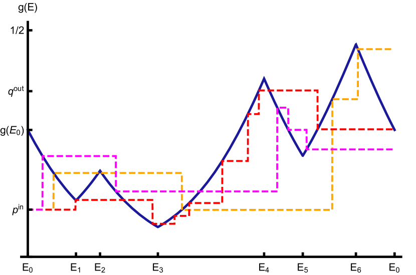
Figure 2: The Gibbs curve (solid) of a general process, alongside examples of different possible paths (dashed), where the thermalization of these different paths occurs at different moments. Note that the $x$-axis represents the evolution of the process with energy levels changed in the following order: $E_{0}\rightarrow E_{1}\rightarrow\ldots\rightarrow E_{0}$.

Basically, we shall prove that most of the transitions are not possible, i.e., that they require some work expenditure. Then it will be very quick to see that all other transitions are achievable.

VII.1 Why the proof of Lemma VI.1 does not generalize, and the idea of the proof in the general case.

As we will show, even in the fully general case, one can divide the process into three parts, two of which (part I and III) are relatively simple, and we shall observe that within them some amount of work is lost with probability bounded away from zero.

Namely, as in the example from the previous section, in stages I and III we will condition on “0” when the level transformation in that part amounts to raising level, and we will condition on “1” when it is lowering level. We shall then show, that this indeed gives some fixed work loss. As a matter of fact the work loss will be, in general, only incurred in stage III.

The main problem will be to show that one cannot regain the work loss of stage III cannot be recovered in stage II.

Let us recall what reasoning regarding this was used in Section VI. With some decent probability (bounded away from zero), the ground state (0) shall be occupied (by the optimal process) in at least half of the steps of part II, which is, in fact, intuitively obvious, since the probability of occupying the lower level in a single step is lower bounded by $1-p^{\mathrm{out}}$. This, in turn, follows from the fact that (i) the Gibbs curve never goes higher than $p^{\mathrm{out}}$ and (ii) the probability of being in the excited state in each step lays on a Gibbs curve (i.e., it is equal to $g(E_{i})$).

While analyzing a general protocol, the above reasoning will not be sufficient. For instance, stage II may consist of parts with either decreasing or increasing excited energy levels. Within the parts, where energy decreases, we can apply the above argument to claim that, with probability bounded away from zero, we gain much less work than needed to regain the losses in stages I and III. On the other hand, while trying to transfer this reasoning to the parts of stage II, during which the energy goes up, we encounter considerable difficulty.

Indeed, suppose that we want to estimate the probability, with which we lose more work than it is indicated by the free energy change, meaning here that the upper level is occupied often enough. Unfortunately, there is no lower bound for the probability of occupying the excited state in a single step ($g(E_{i})$). In fact, it is even close to zero for a sufficiently large $E_{i}$.

We, therefore, see that regarding stage II, no direct generalization of the approach from Section VI can work. However, there is one thing to learn from that case. Namely, in part II we can consider two extreme regimes: the first one, in which $n_{\mathrm{II}}$ is sufficiently large, and the second one, in which $n_{\mathrm{II}}=1$.

For large enough $n_{\mathrm{II}}$, the path of the process (the red one in Fig. 1) is approximately equal to the Gibbs curve. As a consequence, the random variable, which describes the work extracted by the system in stage II, is tightly concentrated around the average, determined here by the area below the Gibbs curve, which is equal to the difference of free energies (with the negative sign) between the initial and final Gibbs state on the part II Gibbs curve.

One can argue then that such a work gain cannot balance the losses incurred in stages I and III.

Now, in the other extreme case, i.e., if $n_{\mathrm{II}}=1$, the random variable, describing the work extracted by the system in stage II, is not concentrated around the Gibbs curve, so we cannot immediately conclude that it is equal or even close to the difference of free energies. Yet, we see that in such a case with constant probability we do not gain work at all, thus for sake of proof of general result we have to find some way to account for it.

While considering a general process, we shall also specify two cases: the one, where the random variable, describing the work extracted by the system in stage II, is to some extent concentrated around $-\Delta F$ (minus the free energy change), and the other one, where it is not. In the first case, we shall use (with some additional tricks) the Chebyshev inequality. In the second case, we shall note, that although the work is not concentrated around $-\Delta F$, it is very badly, but still somehow concentrated around the mean. Now, however, the mean is much smaller than $-\Delta F$, so even very bad concentration around the mean, will imply, via the Cantelli inequality, that with some probability bounded away from zero work is close to $-\Delta F$.

VII.2 Preparations for the proof

For greater clarity, we shall first determine transitions that cannot be done without using CO5 At the end of this section we will outline how to extend the reasoning to include CO5. Our main tool will be the notion of paths.

Paths. Recall, that at each step of the process, one applies thermalization map $\mathcal{C}_{i}=(1-\gamma_{i})\mathbbm{1}+\gamma_{i}\hat{\tau}_{i}$, where $\hat{\tau}_{i}$ is a constant map that replaces the state with a thermal state $\tau_{i}$ of the Hamiltonian $H(E_{i})$, and $\mathbbm{1}$ is identity map.

We will keep track of the maps applied, and their corresponding probabilities. For example, in a two step process $\mathcal{C}_{2}\mathcal{C}_{1}$, one of the maps $\mathbbm{1}\mathbbm{1}$, $\mathbbm{1}\hat{\tau}_{1}$, $\hat{\tau}_{2}\mathbbm{1}$, $\hat{\tau}_{2}\hat{\tau}_{1}$ is applied with corresponding probabilities $(1-\gamma_{2})(1-\gamma_{1})$, $(1-\gamma_{2})\gamma_{1}$, $\gamma_{2}(1-\gamma_{1})$, and $\gamma_{2}\gamma_{1}$ (though the particular values of these probabilities will not be important later).

After $n$ steps, a mixture of various sequences of maps $\mathbbm{1}$ and $\hat{\tau}_{i}$ will have been applied. If we represent the map $\hat{\tau}_{i}$ by $G$ (stemming from “Gibbs”), we obtain sequences of the form $\mathbbm{1}GGG\mathbbm{1}G\mathbbm{1}\mathbbm{1}GG...$ where $\mathbbm{1}$ means that $\mathbbm{1}$ was applied and $G$ means that $\hat{\tau}_{i}$ is applied. Thus a given sequence is such a process, where in each step either nothing happens, or full thermalization occurs. Each particular sequence may produce quite an arbitrary final state, but the mixture of the final states produced by all sequences must be equal to our desired final state $\sigma$.

We will introduce a notion of “paths” (see Fig. 2). A path is the sequence of type

$$\Delta E_{1},X_{1},\Delta E_{2},X_{2},\ldots,\Delta E_{n},X_{n},$$ (33)

where $\Delta E_{i}$ are increments of LT steps of the process, and $X_{i}$ are either $\mathbbm{1}$ or $G$ (i.e., $\hat{\tau}(E_{i})$). Since initial energy is $E_{0}$, we can represent energy increments $\Delta E_{i}$ just by $E_{i}$. The energy achieved in the last step must be then $E_{N}=E_{0}$.

The path can be represented by a polygonal curve, consisting of horizontal parts of length $E_{i}$ and vertical parts denoting thermalization which only occurs when $X_{i}=G$), see Fig. 2. In particular, a subsequence of the sort $E_{1}\mathbbm{1},E_{2},\mathbbm{1},\ldots,E_{k}\mathbbm{1}$ is represented by a horizontal line composed of $k$ shorter segments.

Gibbs curve. For us it will be important to consider, along with the path, the “Gibbs curve”, which is the curve whose value is $g(E)$, i.e., the population of upper level for Gibbs state at energy $E$. In Fig. 2 the Gibbs curve is the solid one. The curve has a property, that the area below it over a given interval is given, up to a sign, by difference of free energy of Gibbs states at the beginning and at the end of the interval.

Path shrinking. Once we have defined path and Gibbs curve, it is convenient to simplify both, without affecting the generality of our considerations. The idea of path shrinking is presented in Fig. 3, and shortly speaking amounts to remove $\mathbbm{1}$’s from the sequences determining the path.

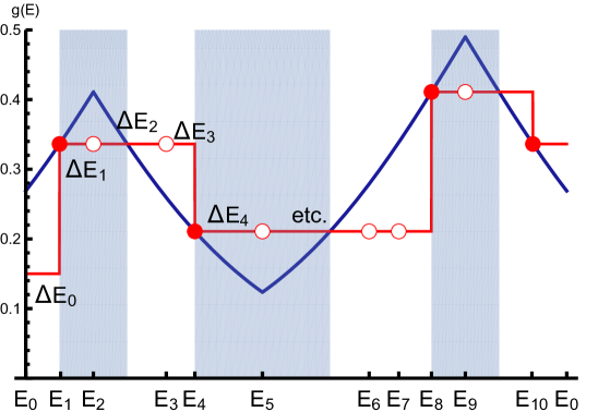
(a) Original

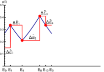
(b) Simplified

Figure 3: Simplifying paths. (a) The paths consist of Level Transformations that change the energy levels by $\Delta E_{i}=(E_{i+1}-E_{i})$, and then at each stage either a thermalization occurred (solid dot) or no thermalization occurred (white dot). Sequences of consecutive transformations without thermalizations are then combined into a single level transformation of the adequate difference $\Delta\tilde{E}_{i}$. Finally, the unnecessary up-down trips are eliminated (shaded regions), with no change to $\Delta\tilde{E}_{i}$. (b) The resulting process, where the $x$-axis energies of the original process are identified for illustration.

Namely, we note that in any path, the sequence of, say, $k$ consecutive $\mathbbm{1}$’s means that there was no thermalization in between level transformations in this part of the path. Therefore, we can glue together those level transformations and obtain a single level transformation with increment $\sum\Delta E_{i}$ which is the sum of the increments in this sequence. Thus without loss of generality, we can consider paths that do not have any more $\mathbbm{1}$’s but consist only level transformations, interlaced with full thermalizations. Sometimes, this will mean that we raise the level and then lower it again, within one level transformation. It is seen in Fig. 3b: the Gibbs curve (that tells us about moves of energy levels) goes up and then down, while path has no thermalization in between. Clearly, it will not affect the work variable. This corresponds to shrinking the path as in Fig. 3b.

Thus, after path shrinking our paths never cross Gibbs curve as a straight line. The only crossings are at thermalization points, and at such crossings, the path changes from being vertical to being horizontal.

Also, after path shrinking, paths correspond to sequences $E_{1},G,E_{2},G,E_{3},G,\ldots,G,E_{N}$. For future investigations we note that the parts of the paths after the first thermalization are actually in one to one correspondence with the sequences of triangle-like areas (the “triangles” are shaded in Fig. 4).

From a single path to the whole process. In our approach, the idea is to focus on a concrete path, and show, that whenever it ends above $g(E_{0})$, then one has to lose work, with some probability bounded away from zero. Then since the mixture of the ends of these paths must be equal to $p^{\mathrm{out}}$ (as the final state is to be $\sigma$), by Markov’s inequality we will get that a decent mass of paths must end up strictly above $g(E_{0})$ and therefore the overall process must cost work with a finite probability.

Single path ending above $g(E_{0})$ loses work. Now let us sketch the idea of how we will prove that a single path ending above $g(E_{0})$ must lose work. There is a natural division of a given path into three stages:

• until the first thermalization

• between first and last thermalization

• after the last thermalization.

In stage I, we shall condition on the event “0” (i.e., occupation of ground state) when the first level transformation goes down, and on the event “1” (occupation of excited state) when it goes up. It will be then not hard to argue that, conditioned on such event, the amount of lost work (denoted by $-W_{\text{I}}$) is no smaller than the free energy difference of the Gibbs state $\Delta F_{\text{I}}$ during stage I. This will be done in Appendix, Lemma A.2 for some range of parameters of input and output states, and for remaining parameters in Appendix, Sections A.3 and A.4.

In stage III, we shall again perform the same conditioning. We shall then prove (which is quite easy) that the amount of lost work (denoted by $-W_{\text{III}}$) will be strictly smaller than the free energy difference of Gibbs state in stage III. The proof is given in the Appendix, Lemma A.3.

Before we move to stage II we shall outline what is the logic behind our rule:

• condition on “0” while lowering level, condition on “1” when raising level.

Namely, such conditioning will imply the largest possible work loss: when we raise levels, the largest work loss is when we occupy upper level and this happens when we condition on “1”. When we lower levels, the smallest work gain is when the level is empty, and this happens when we project onto “0”.

Now, let us note, that since we have cyclic process, i.e., the final Hamiltonian is equal to the initial one, we have:

$$\Delta F_{\text{I}}+\Delta F_{\text{II}}+\Delta F_{\text{III}}=0$$ (34)

(recall, that this is change of free energy of Gibbs states related to temporary Hamiltonian, rather than the actual states). Now, we have just argued above, that

$$-W_{\text{I}}-W_{\text{II}}>\Delta F_{\text{I}}+\Delta F_{\text{III}}+\epsilon_{\text{III}},$$ (35)

where $\epsilon_{\text{III}}$ is some constant (that depends only on input and output states (and the Hamiltonian and temperature). Therefore, if we prove that with some probability $p_{\text{III}}$ we have that

$$-W_{\text{II}}<F_{\text{II}}-\delta$$ (36)

with $\delta\leq\epsilon_{\text{III}}$, then we are done, because combining the formulas (34), (35), and (36) we obtain

$$-(W_{\text{I}}+W_{\text{II}}+W_{\text{III}})>\epsilon_{\text{III}}-\delta>0.$$ (37)

And this occurs with product of the two probabilities of the conditions (one from stage I and the second form stage III) and the probability $p_{\text{II}}$. Let us emphasize here that because the stages I, II and III are separated by thermalizations, the three events are independent, and therefore we can take the product of the probabilities as the probability of the total event.

Thus, the key will now be to show the inequality (36), i.e., that in stage II, with probability bounded away from zero, one gets only a little bit more work than the free energy difference. This is quite challenging. If the work variable was strongly concentrated around the mean, then we could directly make use of some concentration theorems from probability theory. However, the work variable can be far away from the average. In particular, its variance may not be negligible at all. Ultimately, we will use some concentration inequalities, but the reasoning will be much more involved.

To explain our approach to tackle this problem let us consider part of the process in Fig. 4.

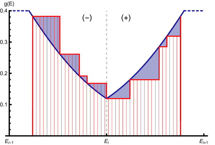
Figure 4: Piece of the general process, where $E_{i-1}<E_{i}$ and $E_{i+1}<E_{i}$. On the right part $E_{i}\rightarrow E_{i+1}$ positive work is drawn, while on the left part $E_{i-1}\rightarrow E_{i}$ negative work is drawn. The area under the curve on the right/left part is positive/negative respectively. The (striped) area below the red curve corresponds to average work, and the (solid) blue area is the difference between $\Delta F$ and average work $\langle W\rangle$.

We depicted there the path in red (note that the path crosses Gibbs only when changing from vertical to horizontal, unlike in the generic path of Fig. 2. In the next section, we shall argue, that one can restrict to such paths without loss of generality). There are two parts: when the Gibbs curve goes up, the energy level goes down, hence work is positive (we denote it by $(+)$). When Gibbs curve goes down, then the level goes up, and the work is negative (this region we denote by $(-)$. Now, the “signed area” below the red curve is average work. Here “signed area” means that in $(-)$ region we take it with minus sign and in $(+)$ we take it with plus sign.

Recall that our goal is to show that with some probability work will be smaller than $\Delta F$ (here $\Delta F$ denotes free energy change for just this part, and ultimately we shall apply the same argument to the whole $\Delta F_{\text{II}}$). To this end, observe that $\Delta F$ is the area below the Gibbs curve. So we obtain

Observation 1.

The average work is smaller than $\Delta F$ by the area $A$ (now standard, not “signed”) of the sum of a triangle like pieces, shaded in blue in Fig. 4.

Indeed, in the $(-)$ part the “signed area” is negative, therefore the free energy difference $\Delta F_{(-)}$ in this part is negative but less negative than the average work $\langle\Delta W_{(-)}\rangle$ in this part just by the area of the “triangles”. In the $(+)$ part the free energy difference is positive, and it is larger than $\langle\Delta W_{(+)}\rangle$ again by the area of “triangles”.

Since we are going to use some concentration inequalities, we are interested in the variance and may want it to be small. Unfortunately, the variance can grow indefinitely. Indeed, in the picture, we see just a piece of the path, while the total process can be an arbitrarily long chain of such pieces. Normally, in statistical physics, a growing variance is fine, because it usually grows with a number of systems like $\sqrt{n}$ while the average grows like $n$. This gives a strong concentration. Here we do not have a priori any such relation.

However we will be able to provide a bound on the work variance in terms of the area of the “triangles” seen in Fig. 4 (in Lemma A.1, Appendix)

Observation 2.

The variance is smaller (up to a constant factor) than the sum of the triangle’s areas.

At a first sight, this would not be helpful, as the area $A$ can be enormous, hence we shall not see any concentration around the average. However note, that we do not want the work $W$ to be close to average. Instead, we want it to be close to $\Delta F$. Due to observation 1, this difference is just the triangles area $A$.

Thus, the larger the area (and therefore the variance), then on the one hand, $W$ becomes less concentrated around the average, but on the other hand, the average is smaller than $\Delta F_{\text{II}}$ and the difference between average work and $\Delta F_{\text{II}}$ increases. Hence we need only a very weak concentration - the deviation can be of the order of $A$.

This is the end of the heuristics that we wanted to present in this section. On the technical side, we will still have to work a bit: it turns out that it is not possible to use a single concentration inequality. For $A$ less than $4/\beta$, we shall use the Chebyshev inequality, while for $A\geq 4/\beta$, the Cantelli inequality has to be used.

VII.3 Adding CO5

Let us now outline the fully general case, where the swaps are allowed. As discussed in previous Section III.2 without loss of generality we can assume that after unitary transformation the system is dephased. Then such an operation is mixture of identity operation and swap operation (that does bit-flip). This means that now path will be determined by sequence of three possible elements:

• Level Transformation (denoted by horizontal line),

• Thermalization (denoted by vertical line ending up at Gibbs curve)

• Swap

Thus a path is the sequence of type

$$\Delta E_{1},X_{1},\Delta E_{2},X_{2},\ldots\Delta E_{n},X_{n},$$ (38)

where, as before, $\Delta E_{1}$ are increments of LT steps of the process, but $X_{i}$ are now either $\mathbbm{1}$ or $G$ (i.e., $\hat{\tau}(E_{i})$) or $S$ representing the $\mathbbm{S}$ operation.

Similarly, as before we can do path shrinking, which now will be not only removing $\mathbbm{1}$’s but also removing pairs of $S$’s, because swap is an involution.

So we consider paths, where $X_{i}$ are either $G$ or $S$. An example of a path is depicted in Fig. 5.

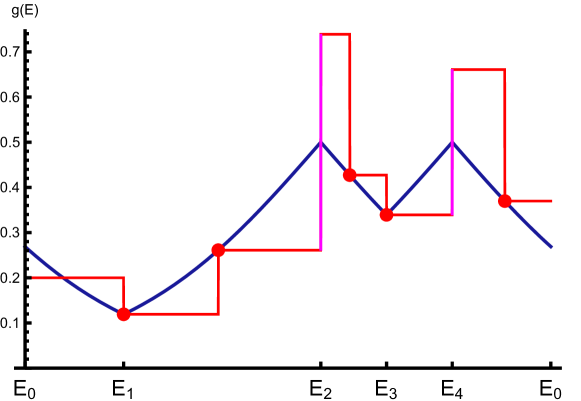
Figure 5: Path with swaps (indicated with pink). Note that swaps can only occur when Gibbs curve has value $1/2$, i.e., when the energy is zero ($E_{2}$ and $E_{4}$ in the example).

As before, the path can be represented by a polygonal curve. Again, $E_{i}$ means that there is horizontal part, $G$ means that there is vertical part ending up at a Gibbs curve, and $S$ means reflection about point $1/2$. This last element can only appear, when also Gibbs curve is at this point, i.e., when energy of upper level is $0$.

To see that $\mathbbm{S}$ causes reflection, no that it transforms state $(1-q,q)$ into $(1-q^{\prime},q^{\prime})$ with $q^{\prime}=1-q$, and one sees that the values $q$ and $q^{\prime}$ are symmetrically positioned with respect to $1/2$, i.e., $(q+q^{\prime})/2=1/2$.

Under swap (similarly like under thermalization) the path can go up or down (which we will loosely denote by swap up and swap down) and this depends on what was the state of the system before the swap. So, if the state was less excited than Gibbs one (i.e., the path was below Gibbs curve) then the operation $\mathbbm{S}$ causes swap up - the path ends up above Gibbs state (actually above $1/2$). When the path was above the Gibbs curve (actually, even above $1/2$ - as swap can be only performed when Gibbs curve is at $1/2$) then the path ends up below Gibbs curve. As said, this is similar to the effect of thermalization, which causes jump up, when the state was below Gibbs curve, and jump down, when it was above. The difference is that thermalization causes the path to end up at Gibbs curve, while $\mathbbm{S}$ performs symmetric reflection about the Gibbs curve.

We shall now argue, that swap down can occur only before first thermalization. To this end, note that swap down can only occur when the path is above $1/2$. However this is only possible after swap up, with perhaps some level transformations, and due to path shrinking, we have excluded such sequences.

Note, that in stage I, i.e., before first thermalization, we may have swap down without previous swap up, because the initial state may have population of excited level greater than $1/2$. And there can be only single such swap up (the second one would need to be after some swap down, which is excluded due to path shrinking).

So we obtain a rule:

• There can be at most one swap up in stage I

• In stage II and III swap down do not occur

The proof now goes along the same lines as discussed before, with some slight complications.

Stages I and III. Concerning stages I and III, we perform quite analogously as in the case without swaps. We again use the rule that we condition on event “0” when Gibbs curve goes up and on “1” when it goes down.

The idea behind such conditioning was that we condition on the most “work loosing” event: when we raise level, then we condition on “1” as then there will be work loss equal to energy change, i.e., largest possible, while when the level is lowered, we condition on “0” and the work gain is zero, i.e., smallest possible.

What happens if swap is performed will be discussed in more detail in Appendix. Here we present just an example, illustrated in Fig. 6.

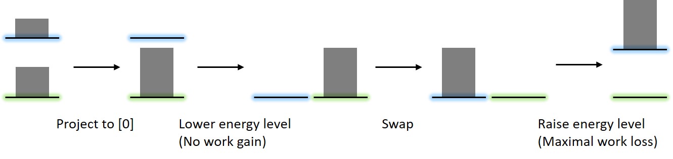
(a) Illustration by means of levels

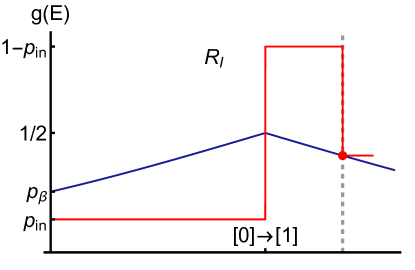
(b) Illustration by means of path

Figure 6: Conditioning on 0 in the swap case.

Suppose that we lower level to zero, perform swap and then raise the level. Then, we see that conditioning on “0” gives the largest work loss: when level is lowered, the work is zero (the smallest possible gain) as, due to our conditioning, the upper state is not populated. Then swap occurs, meaning that the upper level is now fully populated, and during raising the level, maximal work loss is incurred (equal to energy change).

Thus conditioning on “0” after swap changes in to conditioning on “1”, so during the sequence lowering-swap-raising we are all the time in the regime of largest possible work loss.

Stage II. Here the idea is to show that the variance for the path with swaps is bounded by the variance of the suitable path without swaps, that begins and ends at the same point on Gibbs curve. The Lemma B.2 proven in Appendix, does the job.

VII.4 Transitions that are allowed

By the methods outlined above we shall prove in Appendix that except

• (i) the simple transitions coming from admixing a Gibbs state

• (ii) the transitions where initial state is $|0\rangle\langle 0|$ (or, in other notation, $(1,0)$)

all the other transitions are not possible.

The transition of type (i) is just applying CO2 so it is trivially allowed by $\textnormal{{MCO}}_{0}$.

Less trivially, we can also obtain transition of type (ii) by $\textnormal{{MCO}}_{0}$ (actually, by expending strictly no work). Indeed, as said above we can achieve any state more excited than Gibbs just by partial thermalization. Moreover, we can obtain for free (i.e., without spending any work) the ground state by lowering the level to zero, performing the swap, and raising the empty level back to $E_{0}$. Then from the ground state by partial thermalization, we can obtain any state that is less excited than Gibbs.

In this way we obtain

Proposition VII.1.

• It is possible to transform by $\textnormal{{MCO}}_{0}$ state $\rho\coloneqq(1-p^{\mathrm{in}},p^{\mathrm{in}})$ into state $\sigma\coloneqq(1-p^{\mathrm{out}},p^{\mathrm{out}})$ if $p^{\mathrm{in}}\geq p^{\mathrm{out}}\geq p^{\beta}$ or if $p^{\mathrm{in}}\leq p^{\mathrm{out}}\leq p^{\beta}$.

• It is possible to transform state $\rho=(0,1)$ into arbitrary state by means of $\textnormal{{MCO}}_{0}$.

The proposition is also presented in Appendix in the form of Facts B.1 and B.2 together with some discussion.

VIII Conclusions

In this paper, we have shown that without the use of a 2-level auxiliary system the Coarse Operations cannot simulate Thermal Operations. This means that commutative Markovian dynamics cannot simulate Thermal Operations, as one bit of memory is needed. Thus such simulation must be a hidden Markov process, with one-bit space of hidden states. We would like to emphasize, that fully quantum Markovian dynamics in the case of nontrivial Hamiltonian and two level system is effectively noncommutative, as the evolution of diagonal is decoupled from the evolution of the coherences. This is a superselection rules that comes from energy conservation.

In [17] it was shown that an abstract quantum Markovian dynamics (one which does not obey superselection rules), can simulate Thermal Operations. We have thus here established a difference in a continuous dynamics regime, analogous to the difference between Thermal Operations and Gibbs Preserving operations in the quantum operations regime of [21].

In our proof, we could not use directly concentration theorems, as for the general process the work variable can wildly fluctuate. We believe that our analysis may be useful for stochastic control theory, as we were able to work with all possible algorithms of Markovian control over a system of interest.

Possible open questions are about tightening quantitative bounds: namely, what is maximal work loss at a given probability of the loss. One can also consider other measures of the loss, like the average of the work over the region where work is negative, and to minimize such value over all possible processes.

Finally, one may consider an explicit battery, and allow that coherences build up in the intermediate times, while measuring the battery only at the end. It would be even more general setup, where one may try to prove (or disprove) a similar no-go result.

Appendix A Characterization of transitions possible by means of $\textnormal{{MCO}}_{0}$ without CO5

In this section of the Appendix, we will provide a full characterization of the set of transitions that can be done with no work cost by Coarse Operations CO2 and CO3. In the next section, we will expand it by CO5.

A.1 Notation

First, for the convenience of the reader, we will recall some useful definitions and notations from the main part of the paper. As we mentioned in Section III.1, we consider a two-dimensional quantum system with Hamiltonian H parametrized as $H(E)=\text{diag}(0,E)$ where $E\geq 0$. The initial and final Hamiltonians are given by $H(E_{0})$. We also assume that the initial state $\rho=(1-p^{\mathrm{in}},p^{\mathrm{in}})$ and the final state $\sigma=(1-p^{\mathrm{out}},p^{\mathrm{out}})$ are diagonal in the Hamiltonian basis. Furthermore, we consider fixed (inverse) ambient temperatures $\beta>0$. For any given energy $E$, the partition function $Z_{E}$ is given by $Z_{E}=1+e^{-\beta E}$. The thermal state is

$$\tau_{E}=(1-g(E),g(E))$$ (39)

with

$$g(E)=\frac{1}{Z_{E}}e^{-\beta E}.$$ (40)

For any given probability $p$, energy $E(p)$ is defined such that the state $(1-p,p)$ is the Gibbs state with a Hamiltonian $H(E(p))$, i.e.,

$$E(p)=-\frac{1}{\beta}\ln\left(\frac{p}{1-p}\right).$$ (41)

As we already observed, we then have that

$$g(E(p))=p.$$ (42)

We also stated previously (see Section V) that $F(\Psi,E)=\langle E\rangle_{\Psi}-\beta^{-1}S(\Psi)$ is the Helmholtz Free Energy of the state $\Psi$. Additionally, the free energy of the thermal state $\tau_{E}$ corresponding to its Hamiltonian $H(E)$ is given by formula

$$F_{\beta}(E)=g(E)E-\frac{1}{\beta}S(E).$$ (43)

We note that the difference $F(E^{\prime})-F(E)$ can be expressed as

$$F(E^{\prime})-F(E)\coloneqq\int\limits_{E}^{E^{\prime}}g(E)\mathrm{d}E.$$ (44)

In Section III.2 we discussed CO3 operation. $\Delta E_{i}$ denote an energy increment in a single step of this operation, i.e., $H(E_{i+1})=H(E_{i}+\Delta E_{i})$.

Now, let us introduce two variables $\Delta_{i}$ and $q_{i}$ which we will be using later in the proof. These variables are defined as

$$\Delta_{i}\coloneqq|\Delta E_{i}|=|E_{i}-E_{i-1}|$$ (45)

and

$$q_{i}\coloneqq g(E_{i})=\frac{\mathrm{e}^{-\beta E_{i}}}{1+\mathrm{e}^{-\beta E_{i}}}$$ (46)

Let us recall that we defined work to be a random variable with the following distribution:

$$P(W_{i}=-\Delta E_{i})=p_{i},\quad P(W_{i}=0)=1-p_{i},$$ (47)

where $p_{i}$ is the probability of occupying the excited level, and $1-p_{i}$ - the probability of occupying the ground level. Then the total work for an $N$-step process is simply the sum of the work performed in each step:

$$W=\sum_{i=1}^{N}W_{i}.$$ (48)

A.2 The case of initial state being less excited, and the final state being more excited than Gibbs.

In Section VII.2 we introduced a notion of paths. A path is the sequence of type

$$E_{1},X_{1},E_{2},X_{2},\ldots,E_{n},X_{n},$$ (49)

where $E_{i}$ are increments of LT steps of the process, and $X_{i}$ are either $\mathbbm{1}$ or $\hat{\tau}(E_{i})$. The path can be represented by a polygonal curve, consisting of horizontal parts of length $E_{i}$ and vertical parts denoting thermalization which only occurs when $X_{i}=\hat{\tau}(E_{i})$. We also introduced the notion of the Gibbs curve, which is the curve whose value is $g(E)$.

In the following proof, the idea is to focus on a concrete path, and show, that whenever it ends above $g(E_{0})$, then one has to lose work, with some probability bounded away from zero. Then since the mixture of the ends of these paths must be equal to $p^{\mathrm{out}}$ (as the final state is to be $\sigma$), by Markov’s inequality we will get that a decent mass of paths must end up strictly above $g(E_{0})$ and therefore the overall process must cost work with a finite probability.

In the single path scenario, we will show that a single path ending above $g(E_{0})$ must lose work. We will do it by dividing the path into three parts: (I) until the first thermalization, (II) between first and last thermalization, and (III) after the last thermalization.

In part I, we will argue that conditioned on the appropriate event, the amount of lost work (denoted by $-W_{\text{I}}$) is no smaller than the free energy difference of the Gibbs state $\Delta F_{\text{I}}$.

In part III, we will prove that the amount of lost work (denoted by $-W_{\text{III}}$) will be strictly smaller than the free energy difference of Gibbs state $\Delta F_{\text{III}}$.

Finally, in part II we will show that the amount of lost work (denoted by $-W_{\text{II}}$) can be bigger than the free energy difference of Gibbs state $\Delta F_{\text{II}}$. However, by choosing appropriate probability, we can always make the difference between $-W_{\text{II}}$ and $\Delta F_{\text{II}}$ to be smaller than the corresponding one from part II.

To finish the proof it will be enough to combine results for all parts of the path and observe that free energy difference for the whole path is always zero.

A.2.1 Work of the path

In this section we will state three lemmas that bound the work for three parts of the path, which will be denoted by $R$. We will use $p^{\mathrm{in}}$ and $q^{\mathrm{out}}$ to denote the start and endpoints of the path respectively. We will divide the path into three parts $R=(R_{\mathrm{I}},R_{\mathrm{II}},R_{\mathrm{III}})$. The first part $R_{\mathrm{I}}$ ends when thermalization is performed for the first time. The third part $R_{\mathrm{III}}$ starts when thermalization is performed for the last time. For clarity, we will restate that the path is divided into three parts

• until the first thermalization,

• between first and last thermalization,

• after the last thermalization.

Furthermore, this division is also presented in Fig. 7.

Let $\Delta F_{i}$ denote average work of the part of the path that begins in $E_{i}$, ends in $E_{i+1}$, and it approximates (arbitrarily well) the Gibbs curve. It is given by as

$$\Delta F_{i}\coloneqq\int\limits_{E_{i}}^{E_{i+1}}g(E)\mathrm{d}E$$ (50)

For the parts described above we, therefore, obtain

$$\Delta F_{\mathrm{I}}=\int\limits_{\mathrm{I}}g(E)\mathrm{d}E=\int\limits_{E_{0}}^{E_{a}}g(E)\mathrm{d}E,$$ (51)

$$\Delta F_{\mathrm{II}}=\int\limits_{\mathrm{II}}g(E)\mathrm{d}E=\int\limits_{E_{a}}^{E_{b}}g(E)\mathrm{d}E,$$ (52)

$$\Delta F_{\mathrm{III}}=\int\limits_{\mathrm{III}}g(E)\mathrm{d}E=\int\limits_{E_{b}}^{E_{0}}g(E)\mathrm{d}E,$$ (53)

where $a$ is the point where part I ends and part II begins, and $b$ is the point where part II ends and part III begins. Furthermore, let’s observe that

$$\Delta F=\sum_{i}\Delta F_{i}=\sum_{j\in\{\mathrm{I,II,III}\}}\Delta F_{j}=\int\limits_{E_{0}}^{E_{0}}g(E)\mathrm{d}E=0.$$ (54)

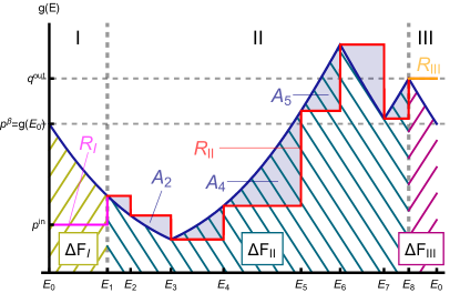
Figure 7: Visualization of different concepts. As mentioned, the path $R$ is divided into three parts $R_{\mathrm{I}},R_{\mathrm{II}},R_{\mathrm{III}}$ which are respectively magenta, red, and orange. Part I begins at $p^{\mathrm{in}}$ and ends at the first thermalization (displayed at $E_{1}$). Part II includes everything from the first thermalization at $E_{1}$ until the very last thermalization at $E_{N}$ ($E_{8}$ in the diagram). Part III is from the moment of the last thermalization until the energy is returned to $E_{0}$. The area underneath the Gibbs curve of the process is $\Delta F=\Delta F_{\mathrm{I}}+\Delta F_{\mathrm{II}}+\Delta F_{\mathrm{III}}$, which are displayed in each part. Finally, during part II the (shaded) areas between the path $R_{\mathrm{II}}$ and the Gibbs curve are the areas $A_{i}$. For ease of visualization, only a subset of these areas is explicitly labeled.

We will denote work of the path as $W=W_{\mathrm{I}}+W_{\mathrm{II}}+W_{\mathrm{III}}$, where $W_{\mathrm{I}},W_{\mathrm{II}}$, and $W_{\mathrm{III}}$ stand for work of each part, respectively. Similarly, the average value of the work (in the limit case where the path approximates the Gibbs curve) is $\Delta F=\Delta F_{\mathrm{I}}+\Delta F_{\mathrm{II}}+\Delta F_{\mathrm{III}}$, where $\Delta F_{\mathrm{I}},\Delta F_{\mathrm{II}}$, and $\Delta F_{\mathrm{III}}$ are average values of each part. Furthermore, by $p^{\beta}$ we will denote the probability level for the Gibbs state at the beginning and end of the process (corresponding to the energy level $E_{0}$). This probability is given by the formula $p^{\beta}=e^{-\beta E_{0}}/{(1+e^{-\beta E_{0}})}$.

Before we are ready to state the three Lemmas about the three parts of the path $R$, we first have to provide a technical Lemma and Corollary that connects the variance of the work with the area under the curve.

Lemma A.1.

The random variable $W_{i}$ describing work satisfies

$$\mathrm{Var}W_{i}\leq\frac{2}{\beta}A_{i}.$$ (55)

where $A_{i}$ is the area between the Gibbs curve and the part of the polygonal chain describing the path (see Fig. 7).

Proof.

Let us denote

$$\Delta_{i}\coloneqq|W_{i}|=|E_{i}-E_{i-1}|,$$ (56)

$$q_{i}\coloneqq g(E_{i})=\frac{\mathrm{e}^{-\beta E_{i}}}{1+\mathrm{e}^{-\beta E_{i}}}.$$ (57)

We first will bound the areas $A_{i}$ by means of triangles with base $\Delta_{i}\equiv|\Delta E_{i}|=|E_{i+1}-E_{i}|$ and height $y_{i}$, see Fig. 8. Namely we have

$$\frac{1}{2}\Delta_{i}y_{i}\leq A_{i}.$$ (58)

Let us now bound the areas of the triangles. We have to consider two cases. First when the Gibbs curve is increasing, we have

$$\frac{y_{i}}{\Delta_{i}}=\frac{\mathrm{d}q}{\mathrm{d}E}(E_{i})=\frac{\mathrm{d}}{\mathrm{d}E}\frac{\mathrm{e}^{-\beta E}}{1+\mathrm{e}^{-\beta E}}(E_{i})=-\frac{\beta\mathrm{e}^{-\beta E_{i}}}{(1+\mathrm{e}^{-\beta E_{i}})^{2}}.$$ (59)

For the decreasing Gibbs curve, we have to estimate a derivative in point $E_{i+1}$ and use the inequality

$$\frac{y_{i}}{\Delta_{i}}=-\frac{\mathrm{d}q}{\mathrm{d}E}(E_{i+1})\leq-\frac{\mathrm{d}q}{\mathrm{d}E}(E_{i})\leq-\frac{\mathrm{d}}{\mathrm{d}E}\frac{\mathrm{e}^{-\beta E}}{1+\mathrm{e}^{-\beta E}}(E_{i})=\frac{\beta\mathrm{e}^{-\beta E_{i}}}{(1+\mathrm{e}^{-\beta E_{i}})^{2}},$$ (60)

$$\Delta_{i}^{2}=2\frac{1}{2}\Delta_{i}y_{i}\frac{\Delta_{i}}{y_{i}}\leq 2A_{i}\frac{(1+\mathrm{e}^{-\beta E_{i}})^{2}}{\beta\mathrm{e}^{-\beta E_{i}}}.$$ (61)

Now, the variance of $W_{i}$ is given by

$$\mathrm{Var}W_{i}=q_{i}(1-q_{i})(\Delta E_{i})^{2}=q_{i}(1-q_{i})\Delta_{i}^{2},$$ (62)

so that we obtain

$$\mathrm{Var}W_{i}=q_{i}(1-q_{i})\Delta_{i}^{2}=\frac{\mathrm{e}^{-\beta E_{i}}}{1+\mathrm{e}^{-\beta E_{i}}}\left(1-\frac{\mathrm{e}^{-\beta E_{i}}}{1+\mathrm{e}^{-\beta E_{i}}}\right)\Delta_{i}^{2}=\frac{\mathrm{e}^{-\beta E_{i}}}{(1+\mathrm{e}^{-\beta E_{i}})^{2}}\Delta_{i}^{2}\leq\frac{2A_{i}}{\beta}.$$ (63)

∎

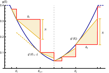
Figure 8: Illustration of how the areas $A_{i}$, which are between the Gibbs curve of the process and the (red) path, are bounded by triangles of base $\Delta_{i}$ and height $y_{i}$. See Lemma A.1 for details.

Corollary A.1.

Since $W$ is the sum of independent random variables $W_{i}$, we can generalize the previous bound in the following way

$$\mathrm{Var}W\leq\frac{2}{\beta}A.$$ (64)

where $W=\sum_{i}W_{i}$,

For the first part of the path $R_{\mathrm{I}}$ we use the following:

Lemma A.2.

It is true that if $p^{\mathrm{in}}<p^{\beta}$, then with probability $p_{\mathrm{I}}\coloneqq p^{\mathrm{in}}$ we have $W_{\mathrm{I}}\leq-\Delta F_{\mathrm{I}}$.

Proof.

First, let us notice that we can assume that the Gibbs curve for the part I of the path is monotonic. If that is not the case we can always use the Path Shrinking method described in Section VII.2. Then we have to consider two cases: (a) decreasing and (b) increasing Gibbs curve (see Figures 9a and 9b respectively). Let us denote by $i_{\textrm{I}}$ the random variable describing the population of the upper level in part I of the path. We shall condition on the even that $i_{\textrm{I}}=1$ in the first case and $i_{\textrm{I}}=0$ in the second case. The probability of such an event equals $1-p^{\mathrm{in}}$ in case (a) or $p^{\mathrm{in}}$ in case (b). Conditioning on that, we always have, for the first part of the path $R_{\mathrm{I}}$, that $W_{\mathrm{I}}=-\Delta E_{\mathrm{I}}\leq-\Delta F_{\mathrm{I}}$. Furthermore, since $p^{\mathrm{in}}<p^{\beta}\leq 1/2$ we know that $p^{\mathrm{in}}<1-p^{\mathrm{in}}$ so we can lower bound probability in both cases using $p^{\mathrm{in}}$. ∎

Remark A.1.

Note, that the inequality in Lemma A.2 cannot be made strict, since we can thermalize just at the beginning, in which case part I becomes trivial, and $W_{\mathrm{I}}=-\Delta F_{\mathrm{I}}=0$.

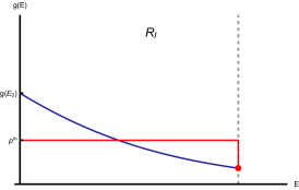
(a)

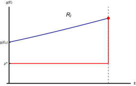
(b)

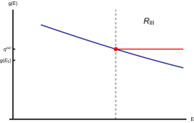
(c)

Figure 9: Different possible behaviors of the path. (a) behavior of the $R_{\mathrm{I}}$ part of the path when Gibbs curve is decreasing. (b) behavior of the $R_{\mathrm{I}}$ part of the path when Gibbs curve is increasing. (c) behavior of the $R_{\mathrm{III}}$ part of the path.

In a similar, a bit more complicated manner, one deals with part of the path $R_{\mathrm{III}}$. We will need the following notation: $E(\cdot)\coloneqq E_{\gamma}$ where $\gamma=(1-\cdot,\cdot)$ for example $E(q^{\mathrm{out}})\coloneqq E_{\gamma}$ where $\gamma=(1-q^{\mathrm{out}},q^{\mathrm{out}})$. We then have the following lemma:

Lemma A.3.

Let

$$\epsilon_{\mathrm{III}}(q^{\mathrm{out}})\coloneqq-E(q^{\mathrm{out}})+E_{0}+\frac{1}{\beta}\ln\frac{1+e^{-\beta E_{0}}}{1+e^{-\beta E(q^{\mathrm{out}})}}.$$ (65)

If $1/2\geq q^{\mathrm{out}}>p^{\beta}\coloneqq e^{-\beta E_{0}}/{(1+e^{-\beta E_{0}})}$, then with probability $p_{\mathrm{III}}\coloneqq q^{\mathrm{out}}$ we have

$$W_{\mathrm{III}}\leq-\Delta F_{\mathrm{III}}-\epsilon_{\mathrm{III}}(q^{\mathrm{out}})$$ (66)

and, furthermore, $\epsilon_{\mathrm{III}}(q^{\mathrm{out}})>0$. Additionally lets us note that $\epsilon_{\mathrm{III}}(p^{\beta})=0$.

Proof.

Let us note that, similarly to the first part of the path we can assume that the Gibbs curve is monotonic also in the third part. It is, again, true due to the Path Shrinking method (see Section VII.2). Furthermore, since the beginning of the path part $R_{\mathrm{III}}$ lies on the Gibbs curve (point of thermalization) and the end is above, the Gibbs curve has to be decreasing (see Fig. 9c). Let us denote by $i_{\textrm{III}}$ the random variable describing the population of the upper level in part III of the path. Then assuming that $i_{\textrm{III}}=1$, what happens with probability $q^{\mathrm{out}}$, we have that

$$W_{\mathrm{III}}=-\Delta E_{\mathrm{III}}=-(E_{0}-E(q^{\mathrm{out}}))=-E_{0}+E(q^{\mathrm{out}})+\Delta F_{\mathrm{III}}-\Delta F_{\mathrm{III}},$$ (67)

where

$$\Delta F_{\mathrm{III}}=-\frac{1}{\beta}\ln\frac{1+e^{-\beta E_{0}}}{1+e^{-\beta E(q^{\mathrm{out}})}}$$ (68)

so

$$W_{\mathrm{III}}\leq-\Delta F_{\mathrm{III}}-\left(-E(q^{\mathrm{out}})+E_{0}+\frac{1}{\beta}\ln\frac{1+e^{-\beta E_{0}}}{1+e^{-\beta E(q^{\mathrm{out}})}}\right)\leq-\Delta F_{\mathrm{III}}-\epsilon_{\mathrm{III}}.$$ (69)

To see that $\epsilon_{\mathrm{III}}$ is strictly positive, note that the it is difference between the rectangular area below horizontal line at the height $1$ (the energy difference) and the area below Gibbs curve (the free energy difference). This is strictly positive, if only the width of the rectangle is not zero, which happens when $E_{0}=E(q^{\mathrm{out}})$, i.e., when $q^{\mathrm{out}}=p^{\beta}$. ∎

For the middle part of the path $R_{\mathrm{II}}$ we can use the following bound:

Lemma A.4.

We have that $W_{\mathrm{II}}\leq-\Delta F_{\mathrm{II}}+\epsilon_{\mathrm{II}}$ with probability $p_{\mathrm{II}}$ where

$$p_{\mathrm{II}}=\min\left\{\frac{2}{3},\frac{\epsilon_{\mathrm{II}}}{\frac{4}{\beta}+\epsilon_{\mathrm{II}}}\right\}.$$ (70)

Proof.

In order to prove this lemma we will consider two cases. Our goal is to show that

$$P(W_{\mathrm{II}}\leq-\Delta F_{\mathrm{II}}+\epsilon_{\mathrm{II}})\geq\min\left\{\frac{2}{3},\frac{\epsilon_{\mathrm{II}}}{\frac{4}{\beta}+\epsilon_{\mathrm{II}}}\right\}.$$ (71)

In the first case we will assume that $A\geq 4/\beta$ where $A$ is area between path the $R_{\mathrm{II}}$ and the Gibbs curve. Then note that

$$\langle W_{\mathrm{II}}\rangle=-\Delta F_{\mathrm{II}}-A.$$ (72)

Indeed, let us divide part II into two further parts - the “$+$” part, where the Gibbs curve goes up (ergo energy goes down), and “$-$” part, where the Gibbs curve goes down (energy goes up). Let $\Delta F_{\mathrm{II}}^{\pm}$ and $W_{\mathrm{II}}^{\pm}$ be the free energy change and work in these subparts. We now note, that $\Delta F_{\mathrm{II}}$ is the integral of Gibbs curve in the range of part II, and $W_{\mathrm{II}}$ is minus the integral of the path over this range. Therefore for those parts of II, where the Gibbs curve is increasing (ergo energy is decreasing) average work $\langle W_{\mathrm{II}}^{+}\rangle$ is equal to area below the path with plus sign. Hence $W_{\textrm{II}}$ is sum of area below Gibbs curve and $A^{+}$, where the latter is the difference between area below Gibbs curve and the area below the path (both with plus sign):

$$\langle W_{\textrm{II}}^{+}\rangle=\text{area below path}=\text{area below Gibbs}-A^{+},$$ (73)

where

$$A^{+}=\text{area below Gibbs}-\text{area below path}\geq 0.$$ (74)

Note that $A^{+}\geq 0$ since for Gibbs curve going up, the path is always below it. On the other hand free energy change $\Delta F_{\mathrm{II}}^{+}$ is equal to area below the Gibbs curve with minus sign. Therefore $\langle W_{\mathrm{II}}^{+}\rangle=-\Delta F_{\mathrm{II}}^{+}-A^{+}$. By analogy we can show that this property also holds for the “-” part, remembering, that in this part path is always above Gibbs curve.

Using Lemma C.2 and Corollary A.1 we obtain:

$$P(W_{\mathrm{II}}\leq-\Delta F_{\mathrm{II}}+\epsilon_{\mathrm{II}})=P(W_{\mathrm{II}}\leq\langle W_{\mathrm{II}}\rangle+A+\epsilon_{\mathrm{II}})\geq\frac{\delta^{2}}{\mathrm{Var}W_{\mathrm{II}}+\delta^{2}}\geq\frac{\delta^{2}}{\frac{2A}{\beta}+\delta^{2}},$$ (75)

where $\delta=A+\epsilon_{\mathrm{II}}$. Using value of delta, we get

$$\frac{\delta^{2}}{\frac{2A}{\beta}+\delta^{2}}\geq\frac{(A+\epsilon_{\mathrm{II}})^{2}}{\frac{2A}{\beta}+(A+\epsilon_{\mathrm{II}})^{2}}\geq\frac{(A+\epsilon_{\mathrm{II}})^{2}}{\frac{2(A+\epsilon_{\mathrm{II}})}{\beta}+(A+\epsilon_{\mathrm{II}})^{2}}=\frac{1}{\frac{2}{\beta(A+\epsilon_{\mathrm{II}})}+1}.$$ (76)

Finally, using the assumption for this case that $A\geq 4/\beta$ we can bound this by

$$\frac{1}{\frac{2}{\beta(A+\epsilon_{\mathrm{II}})}+1}\geq\frac{1}{\frac{2}{\beta\left(\frac{4}{\beta}+\epsilon_{\mathrm{II}}\right)}+1}=\frac{1}{\frac{2}{4+\epsilon_{\mathrm{II}}\beta}+1}\geq\frac{1}{\frac{2}{4}+1}=\frac{2}{3}$$ (77)

which finishes the proof for the first case. In the remaining case we have that $A<4/\beta$. Using Chebyshev’s inequality and again Corollary A.1 we get

$$P(W_{\mathrm{II}}\leq-\Delta F_{\mathrm{II}}+\epsilon)=P(W_{\mathrm{II}}\leq-\Delta F_{\mathrm{II}}-A+\delta)\geq 1-\frac{\mathrm{Var}W_{\mathrm{II}}}{\delta^{2}}\geq 1-\frac{2A}{\beta\delta^{2}}.$$ (78)

When we choose $\delta^{2}=2(A+\epsilon_{\mathrm{II}})/\beta$, we obtain

$$1-\frac{2A}{\beta\delta^{2}}=1-\frac{2A}{\beta\frac{2(A+\epsilon_{\mathrm{II}})}{\beta}}=1-\frac{A}{A+\epsilon_{\mathrm{II}}}=\frac{\epsilon_{2}}{A+\epsilon_{\mathrm{II}}}.$$ (79)

Using the assumption we finally get

$$\frac{\epsilon_{2}}{A+\epsilon_{\mathrm{II}}}\geq\frac{\epsilon_{\mathrm{II}}}{\frac{4}{\beta}+\epsilon_{\mathrm{II}}}.$$ (80)

∎

Now we are ready to combine the above three lemmas into one that describes the work on all three parts of the path $R$.

Lemma A.5.

Let the path $R$ be such that $1/2\geq q^{\mathrm{out}}>p^{\beta}>p^{\mathrm{in}}$. For completeness let us also recall that

$$\epsilon_{\mathrm{III}}(q^{\mathrm{out}})\coloneqq-E(q^{\mathrm{out}})+E_{0}+\frac{1}{\beta}\ln\frac{1+e^{-\beta E_{0}}}{1+e^{-\beta E(q^{\mathrm{out}})}}.$$ (81)

Then the work $W$ of the path $R$ fulfills $W\leq-\epsilon_{\mathrm{III}}(q^{\mathrm{out}})/2$ with probability

$$p=p_{\mathrm{I}}p_{\mathrm{II}}p_{\mathrm{III}}=p^{\mathrm{in}}\min\left\{\frac{2}{3},\frac{\epsilon_{\mathrm{III}}(q^{\mathrm{out}})}{\frac{8}{\beta}+\epsilon_{\mathrm{III}}(q^{\mathrm{out}})}\right\}q^{\mathrm{out}}.$$ (82)

Proof.

Recall that the path $R$ consists of three parts $R=(R_{\mathrm{I}},R_{\mathrm{II}},R_{\mathrm{III}})$ and we denoted the work of the path as $W=W_{\mathrm{I}}+W_{\mathrm{II}}+W_{\mathrm{III}}$ and average values as $\Delta F=\Delta F_{\mathrm{I}}+\Delta F_{\mathrm{II}}+\Delta F_{\mathrm{III}}$.

1. From Lemma A.2 we obtain that $W_{\mathrm{I}}\leq-\Delta F_{\mathrm{I}}$ with probability $p_{\mathrm{I}}\coloneqq p^{\mathrm{in}}$.

2. Then from Lemma A.3 we get that $W_{\mathrm{III}}\leq-\Delta F_{\mathrm{III}}-\epsilon_{\mathrm{III}}(q^{\mathrm{out}})$ with probability $p_{\mathrm{III}}\coloneqq q^{\mathrm{out}}$.

3. Now we can apply Lemma A.4 for $\epsilon_{\mathrm{II}}\coloneqq\epsilon_{\mathrm{III}}(q^{\mathrm{out}})/2$. It gives us that $W_{\mathrm{II}}\leq-\Delta F_{\mathrm{II}}+\epsilon_{\mathrm{II}}=-\Delta F_{\mathrm{II}}+\epsilon_{\mathrm{III}}(q^{\mathrm{out}})/2$ with probability $p_{\mathrm{II}}$ where

   $$p_{\mathrm{III}}\coloneqq\min\left\{\frac{2}{3},\frac{\epsilon_{\mathrm{II}}}{\frac{4}{\beta}+\epsilon_{\mathrm{II}}}\right\}=\min\left\{\frac{2}{3},\frac{\epsilon_{\mathrm{III}}(q^{\mathrm{out}})}{\frac{8}{\beta}+\epsilon_{\mathrm{III}}(q^{\mathrm{out}})}\right\}.$$ (83)

We also know that (see Eq. 54)

$$\Delta F_{\mathrm{I}}+\Delta F_{\mathrm{II}}+\Delta F_{\mathrm{III}}=\Delta F=0.$$ (84)

Combining all of the above together we get that

$$\begin{split}W&=\Delta W_{\mathrm{II}}+\Delta W_{\mathrm{II}}+\Delta W_{\mathrm{III}}\\ &\leq\left(-\Delta F_{\mathrm{I}}\right)+\left(-\Delta F_{\mathrm{II}}+\frac{\epsilon_{\mathrm{III}}(q^{\mathrm{out}})}{2}\right)+\left(-\Delta F_{\mathrm{III}}-\epsilon_{\mathrm{III}}(q^{\mathrm{out}})\right)\\ &=-\Delta F_{\mathrm{I}}+-\Delta F_{\mathrm{II}}+-\Delta F_{\mathrm{III}}-\frac{\epsilon_{\mathrm{III}}(q^{\mathrm{out}})}{2}\\ &=-\frac{\epsilon_{\mathrm{III}}(q^{\mathrm{out}})}{2}.\end{split}$$ (85)

The above occurs with probability

$$p=p_{\mathrm{I}}\,p_{\mathrm{I}}\,p_{\mathrm{III}}.$$ (86)

∎

A.2.2 Combining paths into process

In the previous section we showed under which conditions and with what probability a single path’s work is negative. Now we are ready to combine multiple paths into the process. In the theorem below, we state the main result of our paper. Let us, one more time, recall that

$$\epsilon_{\mathrm{III}}(q^{\mathrm{out}})\coloneqq-E(q^{\mathrm{out}})+E_{0}+\frac{1}{\beta}\ln\frac{1+e^{-\beta E_{0}}}{1+e^{-\beta E(q^{\mathrm{out}})}}.$$ (87)

Theorem A.1.

One cannot transform state $\rho\coloneqq(1-p^{\mathrm{in}},p^{\mathrm{in}})$ into state $\sigma\coloneqq(1-p^{\mathrm{out}},p^{\mathrm{out}})$ by operations CO2 and CO3, where $1/2\geq p^{\mathrm{in}}<p^{\beta}<p^{\mathrm{out}}$ for $p^{\beta}=e^{-\beta E_{0}}/{(1+e^{-\beta E_{0}})}$ without spending the amount of work

$$W\geq\frac{\epsilon_{\mathrm{III}}\left(\frac{p^{\mathrm{out}}+p^{\beta}}{2}\right)}{2}>0$$ (88)

with probability no less than

$$P\left(W\leq-\frac{\epsilon_{\mathrm{III}}\left(\frac{p^{\mathrm{out}}+p^{\beta}}{2}\right)}{2}\right)\geq p_{\mathrm{I}}\,p_{\mathrm{II}}\,p_{\mathrm{III}}\,p_{f}=p^{\mathrm{in}}\min\left\{\frac{2}{3},\frac{\epsilon_{\mathrm{III}}\left(\frac{p^{\mathrm{out}}+p^{\beta}}{2}\right)}{\frac{8}{\beta}+\epsilon_{\mathrm{III}}\left(\frac{p^{\mathrm{out}}+p^{\beta}}{2}\right)}\right\}\frac{p^{\mathrm{out}}+p^{\beta}}{2}\frac{p^{\mathrm{out}}-p^{\beta}}{2}>0.$$ (89)

Proof.

First observe that an arbitrary process can be described by a mixture of paths $\{R_{j}\}_{j\in J}$, each occurring with probability $\lambda_{j}$. We will use $p_{j}^{\mathrm{in}}$ and $q_{j}^{\mathrm{out}}$ to denote the starting and ending points of each path respectively. For the process that transforms state $\rho\coloneqq(1-p^{\mathrm{in}},p^{\mathrm{in}})$ into state $\sigma\coloneqq(1-p^{\mathrm{out}},p^{\mathrm{out}})$ the mixture of paths $\{R^{\prime}_{i}\}_{i\in I}$ has to fulfill

$$\mathop{\forall}_{j\in J}p_{j}^{\mathrm{in}}=p^{\mathrm{in}}$$ (90)

and

$$\sum_{j\in J}\lambda_{j}q_{j}^{\mathrm{out}}=p^{\mathrm{out}}.$$ (91)

Let $Y$ be the random variable defined as $P(Y=q_{j}^{\mathrm{out}})=\lambda_{j}$. Then

$$\mathbf{E}Y=\sum_{j\in J}\lambda_{j}q_{j}^{\mathrm{out}}=p^{\mathrm{out}}.$$ (92)

Since, for all paths, we have that $Y\in[0,1]$, we can use Markov’s inequality in the form (see Lemma C.1 Eq. 121 for details)

$$P(Y>a)\geq 1-\frac{1-\mathbf{E}Y}{1-a}.$$ (93)

Let us choose $a\coloneqq(p^{\mathrm{out}}+p^{\beta})/2$ where

$$p^{\beta}\coloneqq\frac{e^{-\beta E_{0}}}{Z_{E_{0}}}=\frac{e^{-\beta E_{0}}}{1+e^{-\beta E_{0}}}$$ (94)

which gives us

$$P\left(Y>\frac{p^{\mathrm{out}}+p^{\beta}}{2}\right)\geq 1-\frac{1-\mathbf{E}Y}{1-a}=1-\frac{1-p^{\mathrm{out}}}{1-\frac{p^{\mathrm{out}}+p^{\beta}}{2}}=\frac{p^{\mathrm{out}}-p^{\beta}}{2-p^{\mathrm{out}}-p^{\beta}}\geq\frac{p^{\mathrm{out}}-p^{\beta}}{2}\eqqcolon p_{f}.$$ (95)

From Lemma A.5 we know that for each path $R_{j}$ such that $q_{j}^{\mathrm{out}}>(p^{\mathrm{out}}+p^{\beta})/2$ the work of the path fulfills

$$W\leq-\frac{\epsilon_{\mathrm{III}}\left(\frac{p^{\mathrm{out}}+p^{\beta}}{2}\right)}{2}$$ (96)

with probability

$$p_{\mathrm{I}}\,p_{\mathrm{II}}\,p_{\mathrm{III}}=p^{\mathrm{in}}\min\left\{\frac{2}{3},\frac{\epsilon_{\mathrm{III}}\left(\frac{p^{\mathrm{out}}+p^{\beta}}{2}\right)}{\frac{8}{\beta}+\epsilon_{\mathrm{III}}\left(\frac{p^{\mathrm{out}}+p^{\beta}}{2}\right)}\right\}\frac{p^{\mathrm{out}}+p^{\beta}}{2}.$$ (97)

One additional thing, we should point out here is that part III of the paths that construct the process always exist in this case and it is nontrivial. ∎

To give some examples we show plot of work and probability for different values $p^{\mathrm{out}}$ from Theorem A.1 in Fig. 10. We choose there specific situation where $\beta=1$ $p^{\beta}=1/4$ and $p^{\mathrm{in}}\in\{1/16,1/8,3/16\}$. However, note that the work do not depends on value of $p^{\mathrm{in}}$. Furthermore, probability for different values of $p^{\mathrm{in}}$ is only affected by just multiplication by appropriate $p^{\mathrm{in}}$.

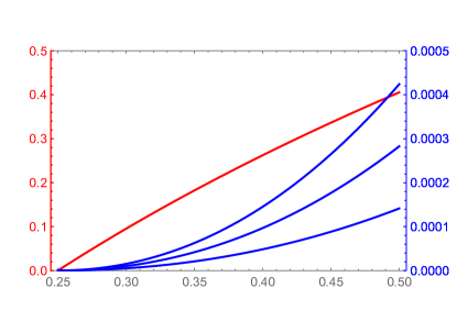
Figure 10: Lost work - red line and probability - blue lines ($p^{\mathrm{in}}\in\{1/16,1/8,3/16\}$ from bottom to top) for case where $\beta=1$, $p^{\beta}=1/4$, and $p^{\mathrm{out}}\in(1/4,1/2)$.

A.3 The case of initial state that is less excited and final state that is more excited than Gibbs state

Now we will consider the opposite situation when we want to transform state that is “above” Gibbs into state “below” Gibbs. Formally we state it below as theorem after introducing $\tilde{\epsilon}$ value given by

$$\tilde{\epsilon}_{\mathrm{III}}(q^{\mathrm{out}})\coloneqq E(q^{\mathrm{out}})-E_{0}+\frac{1}{\beta}\ln\frac{1+e^{-\beta E_{0}}}{1+e^{-\beta E(q^{\mathrm{out}})}}.$$ (98)

Theorem A.2.

One cannot transform state $\rho\coloneqq(1-p^{\mathrm{in}},p^{\mathrm{in}})$ into state $\sigma\coloneqq(1-p^{\mathrm{out}},p^{\mathrm{out}})$ where $1/2\geq p^{\mathrm{out}}<p^{\beta}<p^{\mathrm{in}}\leq 1$ for $p^{\beta}=e^{-\beta E_{0}}/{(1+e^{-\beta E_{0}})}$ without spending the amount of work

$$W\geq\frac{\tilde{\epsilon}_{\mathrm{III}}\left(\frac{p^{\mathrm{out}}+p^{\beta}}{2}\right)}{2}>0$$ (99)

with probability no less than

$$P\left(W\leq-\frac{\tilde{\epsilon}_{\mathrm{III}}\left(\frac{p^{\mathrm{out}}+p^{\beta}}{2}\right)}{2}\right)\geq p_{\mathrm{I}}\,p_{\mathrm{II}}\,p_{\mathrm{III}}\,p_{f}=\min\{p^{\mathrm{in}},1-p^{\mathrm{in}}\}\min\left\{\frac{2}{3},\frac{\tilde{\epsilon}_{\mathrm{III}}\left(\frac{p^{\mathrm{out}}+p^{\beta}}{2}\right)}{\frac{8}{\beta}+\tilde{\epsilon}_{\mathrm{III}}\left(\frac{p^{\mathrm{out}}+p^{\beta}}{2}\right)}\right\}\left(1-\frac{p^{\mathrm{out}}+p^{\beta}}{2}\right)\frac{p^{\beta}-p^{\mathrm{out}}}{2}>0,$$ (100)

where

$$\tilde{\epsilon}_{\mathrm{III}}\left(\frac{p^{\mathrm{out}}+p^{\beta}}{2}\right)=-\Delta F_{\mathrm{III}}$$ (101)

since we us projection on 0 in the part III of the path in this case.

Since this theorem is a close analog of Theorem A.1 we will only provide a sketch of the proof showing the main differences.

Proof.

By analogy, to the case described in the theorem and lemmas above, we can use similar arguments. We can again use version of Markov’s inequality (see Lemma C.1 Eq. (120)) to show that with some probability paths of the process are ending below $p^{\beta}$. Namely

$$P\left(Y<\frac{p^{\mathrm{out}}+p^{\beta}}{2}\right)\geq 1-\frac{\mathbf{E}Y}{a}=1-\frac{p^{\mathrm{out}}}{\frac{p^{\mathrm{out}}+p^{\beta}}{2}}=\frac{p^{\beta}-p^{\mathrm{out}}}{p^{\beta}+p^{\mathrm{out}}}\geq\frac{p^{\beta}-p^{\mathrm{out}}}{2}\eqqcolon p_{f}.$$ (102)

For each path $R$ we can use the same division into three parts $R=(R_{\mathrm{I}},R_{\mathrm{II}},R_{\mathrm{III}})$. Furthermore, all arguments from Lemma A.5 will also apply if we can obtain appropriate bounds for all three parts. It is important to notice that the middle part $R_{\mathrm{II}}$ is the same as in the previous case so we can apply Lemma A.4 directly. So the only key difference is behavior in the first ($R_{\mathrm{I}}$) an third ($R_{\mathrm{III}}$) part of the path. In the first part ($R_{\mathrm{I}}$) we can use an analog of the proof of Lemma A.2. Again, for decreasing Gibbs curve (see Fig. 11a) we take $i_{\mathrm{I}}=0$ and $i_{\mathrm{I}}=1$ for the increasing one (see Fig. 11b). Finally, we can also use results of Lemma A.3 observing that now the Gibbs curve has to be increasing instead of decreasing in the part $R_{\mathrm{III}}$ of the path (see Fig. 11c). In this case we assume that $i_{\mathrm{III}}=0$ what happens with probability $1-q^{\mathrm{out}}$. The probability of Eq. (100) is strictly positive, because $p^{\beta}>p^{\mathrm{out}}$, and by definition $p^{\beta}\leq 1/2$. One additional thing, we should point out here is that part III of the paths that construct the process always exist in this case and it is nontrivial. Furthermore, this is not true if $p^{\mathrm{in}}=1$ so the theorem have to exclude that special situation. ∎

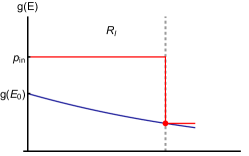
(a)

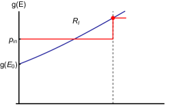
(b)

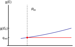
(c)

Figure 11: Transition from $p_{\beta}\leq p^{in}\leq\frac{1}{2}$ and $q^{out}\leq p_{\beta}$.

A.4 Other cases of transformations that can not be achieved

In this section, we will discuss the cases when the initial and the final states are on the same side of the Gibbs curve and the final state is further away from the Gibbs state than the initial state.

Theorem A.3.

One cannot transform state $\rho\coloneqq(1-p^{\mathrm{in}},p^{\mathrm{in}})$ into state $\sigma\coloneqq(1-p^{\mathrm{out}},p^{\mathrm{out}})$ when $p^{\beta}\leq p^{\mathrm{in}}<p^{\mathrm{out}}$ or when $p^{\beta}\geq p^{\mathrm{in}}>p^{\mathrm{out}}$ for $p^{\beta}=e^{-\beta E_{0}}/{(1+e^{-\beta E_{0}})}$ without spending some positive amount of work with positive probability.

Proof.

Proof of this theorem is the direct application of appropriate parts of the proofs of Theorem A.1 and Theorem A.2. Depending on the situation (if the initial state if above or below the initial Gibbs state) we can apply appropriate reasoning for the part I of the path obtaining that $W_{\mathrm{I}}\leq-\Delta F_{\mathrm{I}}$. Similarly, we can use appropriate facts for final state and part III obtaining that $W_{\mathrm{III}}\leq-\Delta F_{\mathrm{III}}-\epsilon_{\mathrm{III}}(q^{\mathrm{out}})$ (or $\tilde{\epsilon}$ depending on the case). Part II is the same as in previous proof and gives us that $W_{\mathrm{II}}\leq-\Delta F_{\mathrm{II}}+\epsilon_{\mathrm{II}}$. Finally, using once again reasoning from previous theorems (combining paths into processes and using an appropriate version of Markov inequality) we can show that with positive probability we will lose more work in part III than we can gain in part II. It implies that the state transformation is impossible without spending some amount of work. ∎

It is also interesting to note that the above transformations also cannot be performed by Thermal Operations (TO). Indeed, Thermal Operations can sometimes swap the states “through” Gibbs one, but they cannot move away from Gibbs state.

Appendix B Characterization of transitions possible by means $\textnormal{{MCO}}_{0}$

In this Appendix, we will provide a full characterization of the set of transitions that can be done with no work cost by Coarse Operations without auxiliary systems namely and work expenditure, i.e., by operations $\textnormal{{MCO}}_{0}$. This means that we have to discuss the most generals case, where CO5 operations are allowed. As discussed in Section VII.3 we have to consider paths that include swaps. The paths will then have a new element - reflection about the point $1/2$. It can only appear when the upper level has energy 0, i.e., when the Gibbs curve is at $1/2$. Moreover, we argued, that after path shrinking, the “swap up” can only occur in stage $I$.

Now we shall show, that in most cases, the new setup can be reduced to the old one, in the sense that the work loss will be no smaller than for the path without swaps.

We will consider all possible cases when the swap operator is used. To maintain clarity, we will divide them based on in which part of the path (I, II, or III) the swap operator is performed:

• Swap performed in part I (i.e., before first thermalization). We can distinguish here three cases depending on the starting point of the path. The first in which $p^{\beta}<p^{\mathrm{in}}<1/2$ is presented in the Fig. 12a. The second one in which $p^{\mathrm{in}}>1/2$ is displayed in Fig. 12b. Finally, the third when $p^{\mathrm{in}}<p^{\beta}$ is depicted in the Fig. 12c.

  

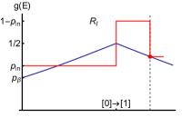
  (a)

  

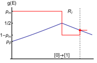
  (b)

  

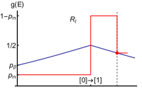
  (c)

  

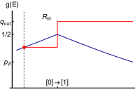
  (d)

  Figure 12: Additional possibilities coming from “swap”. For part I we have three possible cases: a) the case $R_{\text{I}}$ with $p_{\beta}\leq p^{in}\leq 1/2$ b) the case $p^{in}\geq 1/2$ c) the case $p^{in}\leq p_{\beta}$. For part III there is one case: d) $q^{out}\geq 1/2$.

• Swap operation is performed in part II.

• Swap is performed in part III (i.e., after the last thermalization). Here we have only one case we have to consider namely when $q^{\mathrm{out}}>1/2$. It is because when we perform swap operation after the last thermalization the path is always above 1/2. Furthermore, performing the swap after the last thermalization is the only possible way to achieve such a final state. We can see that in Fig. 12d.

Let us first discuss item (ii), i.e., the part II. We want to show that even in presence of swaps, the general Lemmas A.1 and A.4 still hold. Actually, it is enough to show that the analogue of Lemma A.1 holds, as the other lemma is an abstract one, that bases on the former one. To do so we will firstly introduce random variable that that describe work in situation when swap is performed in between thermalizations in part II

$$W\coloneqq\begin{cases}-\Delta E_{2},i=0\mapsto 1,1-q\\ -\Delta E_{1},i=1\mapsto 0,q\end{cases}.$$ (103)

Then the expected value of work equals

$$\langle W\rangle=q(-\Delta E_{1})+(1-q)(-\delta E_{2})$$ (104)

and variance of work is

$$\begin{split}\mathrm{Var}W=&\langle W^{2}\rangle-\langle W\rangle^{2}\\ =&q(-\Delta E_{1}^{2})+(1-q)(-\Delta E_{2}^{2})-(q(-\Delta E_{1})+(1-q)(-\Delta E_{2}))^{2}\\ =&q(1-q)\Delta E_{1}^{2}+q(1-q)\Delta E_{2}^{2}+q(1-q)|\Delta E_{1}||\Delta E_{2}|.\end{split}$$ (105)

Our goal is to show that above variance is upper bounded by area between the Gibbs curve and the the process path, like in Lemma A.1. The first part in last line of Eq. (105) is upper bounded by $2A_{1}/\beta$ just like in Lemma A.1 (where $A_{1}$ is triangle-like area depicted in Fig. 13. For the second part of last line of Eq. (105) we have that $q(1-q)\Delta E_{2}^{2}\leq 1/2(1-1/2)\Delta E_{2}^{2}$. Now, we note that the relevant triangle starts at the point, where $q=1/2$. Hence we can again use Lemma A.1, obtaining that $q(1-q)\Delta E_{2}^{2}\leq 2A_{2}/\beta$.

So what remains, is to show that third part of the equation is not greater than the area of green rectangle from Fig. 13.

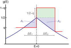
Figure 13: Diagram for Lemma B.1.

Lemma B.1.

It is true that

$$2q(1-q)\Delta_{1}\Delta_{2}\leq\frac{2}{\beta}\left(\frac{1}{2}-q\right)\Delta_{2}$$ (106)

, where $\Delta_{1}=|\Delta E_{1}|$, $\Delta_{2}=|\Delta E_{2}|$. Note that $\left(\frac{1}{2}-q\right)\Delta_{2}$ appearing on the right-hand-side is the area of green rectangle from Fig. 13.

Proof.

Our goal is to show that

$$2q(1-q)\Delta_{1}\Delta_{2}\leq\frac{2}{\beta}\left(\frac{1}{2}-q\right)\Delta_{2}.$$ (107)

After simplification we have that

$$q(1-q)\Delta_{1}\leq\frac{\frac{1}{2}-q}{\beta}$$ (108)

and later that

$$\beta q(1-q)\Delta_{1}\leq\frac{1}{2}-q.$$ (109)

Let $x\coloneqq\beta\Delta_{1}$. We also know that $q\coloneqq e^{-x}/(1+e^{-x})$. Hence, we obtain

$$\frac{e^{-x}}{1+e^{-x}}\left(1-\frac{e^{-x}}{1+e^{-x}}\right)x\leq\frac{1}{2}-\frac{e^{-x}}{1+e^{-x}}$$ (110)

and

$$\frac{e^{-x}}{(1+e^{-x})^{2}}x\leq\frac{1-e^{-x}}{2(1+e^{-x})}$$ (111)

therefore

$$\frac{e^{-x}}{1+e^{-x}}x\leq\frac{1-e^{-x}}{2}$$ (112)

which is equivalent to

$$xe^{-x}\leq\frac{1-(e^{-x})^{2}}{2}$$ (113)

or to

$$x\leq\frac{e^{x}(1-e^{-2x})}{2}.$$ (114)

Using definition of hyperbolic function we can finally write

$$x\leq\frac{e^{x}-e^{-x}}{2}=\sinh{x}.$$ (115)

We thus want to have

$$x\leq\sinh{x}$$ (116)

what is true for $x>0$. In order to show last inequality it is enough to observe that $\sinh 0=0$ and that

$$\frac{\mathrm{d}}{\mathrm{d}x}(\sinh{x}-x)=\cosh{x}-1>0$$ (117)

for all $x>0$. ∎

We have thus shown that even in presence of swaps, variance is still bounded above as in Lemma A.1:

Lemma B.2.

Consider arbitrary path in stage I and denote by $\tilde{A}$ the area enclosed by the path and Gibbs curve. Then the work variance satisfies

$$VarW\leq\frac{2}{\beta}\tilde{A}.$$ (118)

The area $\tilde{A}$ has again the same interpretation as $A$ in the case of paths without swaps so that Lemma A.4 holds, and therefore we are done with part II.

Now we turn to parts I and III. Once we have described all possible situations in with swap operation can occur, we will argue why the work is not greater than in the no swaps scenario. In the cases described in items (i) depicted in Fig. 12a and 12c we can see that there is more negative work than in the scenario without swap. It is because, as we mentioned, the swap is always at a maximum of the Gibbs curve in the point when the “$-$” part starts. Thus, since the path in the case when the swap was performed is above the path without swap, the work is never greater in presence of swap. Alternatively, one can notice, that the work can be bounded from above by zero, exactly as in the case of no swaps.

Note that we consider only one “$+$” part and one “$-$” part. Indeed, we do not need to analyze the possible subsequent “$+$” part since we can always use the Path Shrinking method to discard it.

The case of item (i) depicted in Fig. 12b we have to consider separately. In this case, we will use the fact that swap operation changes the random variable describing the population of the upper level. Because of this, if we assume that $i_{\mathrm{I}}=1$ before the swap then $i_{\mathrm{I}}=0$ after the swap. Therefore, conditioning on the initial value of the population of the upper level to be $1$ we obtain the amount of work can be bounded from above by zero, as in the no swaps case.

In the remaining case (see Fig. 12d) we have with probability $p^{\mathrm{out}}>1/2$ that $\Delta W_{\mathrm{III}}=-E_{0}$ and $\Delta F_{\mathrm{III}}\leq E_{0}/2$. From that we obtain

$$\Delta W_{\mathrm{III}}=-E_{0}\leq-\frac{E_{0}}{2}-\frac{E_{0}}{2}\leq-\Delta F_{\mathrm{III}}-\frac{E_{0}}{2}.$$ (119)

Then $E_{0}/2$ represents the negative work that we need in part III.

In this way we have proved

Statement B.1.

The results of Theorems A.1, A.2 A.3 hold also for transformations CO2,CO3 and CO5, with perhaps different but still positive probability, and the work to be spent.

To finish the characterization, we show below what states can be transformed by $\textnormal{{MCO}}_{0}$.

Fact B.1.

It is possible to transform state $\rho\coloneqq(1-p^{\mathrm{in}},p^{\mathrm{in}})$ into state $\sigma\coloneqq(1-p^{\mathrm{out}},p^{\mathrm{out}})$ if $p^{\mathrm{in}}\geq p^{\mathrm{out}}\geq p^{\beta}$ or if $p^{\mathrm{in}}\leq p^{\mathrm{out}}\leq p^{\beta}$.

It is possible because such a state can be obtained as a mixture of identity operation (no thermalization and no swap) and operation that has only one thermalization at the very beginning of the process (and also no swaps). To understand why it is possible and why it is not contrary to previous theorems, we should note that in this case part III of the path can be trivial. Since there is no part III there is no negative work that comes from this part.

Fact B.2.

It is possible to transform state $\rho\coloneqq(0,1)$ into any state.

Indeed, as in the previous remark, we can achieve any state more excited than Gibbs just by partial thermalization. Moreover, we can obtain for free (i.e., without spending any work) the ground state by lowering the level to zero, performing the swap, and raising the empty level back to $E_{0}$. Then from the ground state by partial thermalization, we can obtain any state that is less excited than Gibbs.

Note that this does not contradict our all previous no-go results, since there was part III, which is absent here. Indeed, part III is mandatory only when we thermalize after changing the Hamiltonian. In case $p^{\mathrm{in}}=1$ we have avoided this.

Appendix C Lemmas from probability theory

Lemma C.1.

Let $Y$ be random variable that takes values from the set $[0,1]$. Then

$$P(Y<a)\geq 1-\frac{\mathbf{E}Y}{a}$$ (120)

and

$$P(Y>a)\geq 1-\frac{1-\mathbf{E}Y}{1-a}.$$ (121)

Proof.

The first inequality is direct application of Markov’s inequality

$$P(Y\geq a)\leq\frac{\mathbf{E}Y}{a}.$$ (122)

For the second one lets define random variable $X=1-Y$. It is easy to see that $X$ takes values from the set $[0,1]$ and that $\mathbf{E}X=1-\mathbf{E}Y$. From Markov’s inequality for $X$ we get that

$$P(X\geq b) \leq\frac{\mathbf{E}X}{b},$$ (123)

$$P(X<b) \geq 1-\frac{\mathbf{E}X}{b},$$ (124)

$$P(1-Y<b) \geq 1-\frac{\mathbf{E}(1-Y)}{b},$$ (125)

$$P(Y>1-b) \geq 1-\frac{1-\mathbf{E}Y}{b}.$$ (126)

Using substitution $a\coloneqq 1-b$ we finally obtain that

$$P(Y>a)\geq 1-\frac{1-\mathbf{E}Y}{1-a}.$$ (128)

∎

Lemma C.2 (Cantelli’s inequality).

Let $X$ be a random variable with expected value $\mathbf{E}X$ and variance $\mathrm{Var}X$. Then for all $\delta>0$,

$$P(X\geq\mathbf{E}X+\delta)\leq\frac{\mathrm{Var}X}{\mathrm{Var}X+\delta^{2}}.$$ (129)

For our purpose we will use slightly different version of inequality

$$P(X\leq\mathbf{E}X+\delta)\geq\frac{\delta^{2}}{\mathrm{Var}X+\delta^{2}}.$$ (130)