Scaling up Differentially Private Deep Learning with Fast Per-Example Gradient Clipping

Abstract

Recent work on Renyi Differential Privacy has shown the feasibility of applying differential privacy to deep learning tasks. Despite their promise, however, differentially private deep networks often lag far behind their non-private counterparts in accuracy, showing the need for more research in model architectures, optimizers, etc. One of the barriers to this expanded research is the training time — often orders of magnitude larger than training non-private networks. The reason for this slowdown is a crucial privacy-related step called “per-example gradient clipping” whose naive implementation undoes the benefits of batch training with GPUs. By analyzing the back-propagation equations we derive new methods for per-example gradient clipping that are compatible with auto-differeniation (e.g., in PyTorch and TensorFlow) and provide better GPU utilization. Our implementation in PyTorch showed significant training speed-ups (by factors of 54x - 94x for training various models with batch sizes of 128). These techniques work for a variety of architectural choices including convolutional layers, recurrent networks, attention, residual blocks, etc.

1 Introduction

Machine learning models trained on sensitive datasets, such as medical records, emails, and financial transactions have great value to society but also pose risks to individuals who contributed their information to the training data. Even if the model parameters are not shared, black-box access to the models can leak private information [40]. Differential privacy is a promising framework for mitigating such risks because of its strong mathematical guarantees and because of recent advances in differentially private training of predictive models.

Simple models, such as linear regression and logistic regression, which have convenient mathematical structures (e.g., convexity) and relatively few parameters, have been well-studied in the differentially private literature and many privacy preserving training algorithms have been proposed (e.g., [10, 24, 7, 21, 51, 45, 26, 12, 35]). These algorithms are generally fast and accurate compared to their non-private counterparts.

However, state-of-the-art prediction results generally come from deep artificial neural networks with millions of parameters. These models are not convex and hence require different fitting algorithms to ensure privacy [2, 32, 23, 50]. In the non-private case, training is generally accomplished using stochastic gradient descent backed by GPU/TPU hardware accelerators that process multiple training records together in a batch. In the privacy-preserving case, the most generally applicable training algorithm is also a variation of stochastic gradient descent [2]. However, its current implementations (e.g., [31]) are extremely slow because a key step, “per-example gradient clipping”, limits the batch-processing capabilities of GPUs/TPUs, resulting in slowdowns of up to two orders of magnitude. This slowdown has a direct impact on differentially-private deep learning research, as it becomes expensive even to experiment with differential privacy and different neural network architectures [6].

In this paper, we show that most of this slowdown can be avoided. By analyzing how backpropagation computes the gradients, we derive some tricks for fast per-example-gradient clipping that are easy to implement and result in speedups of up to 94x over the naive approach. These methods take advantage of auto-differentiation features of standard deep learning packages (such as TensorFlow and PyTorch [33]) and do not require any low-level programming (our code consists of Python wrappers around PyTorch layer objects — e.g., a wrapper for fully connected layers, a wrapper for convolutional layers, etc.).

We note that Goodfellow [17] provided a fast per-example gradient clipping method that only applied to fully connected networks. Our results apply to a wider variety of architectures, including convolutional layers, recurrent networks, attention, residual blocks, etc.

In short, our contributions are as follows.

• We present methods for efficiently computing per-example gradients for different kinds of deep learning models, achieving a speedup of up to 54x to 94x (depending on the model) compared to naive per-example gradient computation on mini-batches of size 128. This allows hardware-accelerated differentially private training of deep learning models to rival the speed of hardware-accelerated non-private training and thus makes differentially private deep learning possible in practical timeframes.

• The proposed methods do not require fundamental changes to GPU parallelization. Instead, they are easy to implement because they take advantage of automatic differentiation capabilities of modern deep learning packages. Our PyTorch wrappers are being prepared for open-source release.

• As an application of the proposed framework, we demonstrate how to train (under Rényi differential privacy) a Transformer encoder block [44], a key component in an architecture that has lead to recent advances in natural language processing.

• We perform extensive experiments and empirically show the effectiveness of approach for differentially private training of various kinds of deep neural network models.

The rest of this paper is organized as follows. In Section 2, we define notations and provide background on differential privacy. Building on these concepts, we describe the per-example gradient clipping problem in Section 3. We then discuss related work in Section 4. We present our proposed methods in Section 5, experimental results in Section 6 and conclusions in Section 7.

2 Preliminaries

In this paper, we use upper-letters (e.g., $W$) to represent matrices, bold-face lower-case (e.g., $\mathbf{x}$) to represent vectors and non-bold lower-case (e.g., $y$) to represent scalars. One exception is that $D$ represents a dataset. Tensors of order 3 or higher (i.e., multidimensional arrays that are indexed by 3 or more variables) are represented in calligraphic font (e.g,. $\mathcal{W}$).

We index vectors using square brackets (e.g., $\mathbf{x}[1]$ is the first component of the vector $\mathbf{x}$. For matrices, we use subscripts to identify entries ($W_{i,j}$ is the entry in row $i$, column $j$). Similarly, tensors are indexed using subscripts (e.g., $\mathcal{W}_{i,j,k}$ is the entry at row $i$, column $j$, depth $k$). To partially index a matrix or tensor, we use the symbol $*$. That is row $i$ in a matrix $W$ is $W_{i,*}$, column $j$ is $W_{*,j}$. Similarly, for a 4th order tensor $\mathcal{W}$, $\mathcal{W}_{i,j,*,*}$ is a matrix $V$ where $V_{k,\ell}=\mathcal{W}_{i,j,k,\ell}$.

Let $D=\{(\textbf{x}_{1},y_{1}),\ldots,(\textbf{x}_{n},y_{n})\}$ be a set of $n$ records, where $\textbf{x}_{i}\in\mathfrak{X}$ is a feature vector and $y_{i}\in\mathfrak{Y}$ is a target (value we must learn to predict). We say two datasets $D$ and $D^{\prime}$ are neighbors if $D^{\prime}$ can be obtained from $D$ by adding or removing one record and write $D{\sim}D^{\prime}$ to denote this relationship.

2.1 Differential Privacy

Differential privacy is a widely accepted formal privacy definition that requires randomized algorithms (also called mechanisms to process data. The intuition behind it is that the addition/deletion of one record should have very little influence on the output distribution.

Definition 1 (($\epsilon,\delta$)-DP [16, 15]).

Given privacy parameters $\epsilon\geq 0$, $\delta\geq 0$, a randomized mechanism (algorithm) $\mathcal{M}$ satisfies ($\epsilon,\delta$)-differential privacy if for every set $S\subseteq\operatorname{range}(\mathcal{M})$ and for all pairs of neighboring datasets $D{\sim}D^{\prime}$,

$$\Pr[\mathcal{M}(D)\in S]\leq\exp(\epsilon)\Pr[\mathcal{M}(D^{\prime})\in S]+\delta\,.$$

The probability only depends to the randomness in $\mathcal{M}$.

The cases $\delta=0$ and $\delta>0$ are respectively referred to as pure and approximate differential privacy.

2.2 Rényi Differential Privacy

One of the drawbacks of Definition 1 is that accurately tracking privacy loss from multiple noise-infused accesses to the data is difficult. For this reason, most work on differentially private deep learning uses a variant called Rényi Differential Privacy (RDP) [29] to track privacy leakage of an iterative algorithm and then. At the very end, the RDP parameters are converted to the $\epsilon,\delta$ parameters of Definition 1. RDP relies on the concept of Rényi divergence:

Definition 2 (Rényi Divergence).

Let $P_{1}$ and $P_{2}$ be probability distributions over a set $\Omega$ and let $\alpha\in(1,\infty)$. Rényi $\alpha$-divergence $\operatorname{\mathfrak{D}}_{\alpha}$ is defined as: $\operatorname{\mathfrak{D}}_{\alpha}(P_{1}\;\|\;P_{2})=\frac{1}{\alpha-1}\log(\operatorname{\mathbb{E}}_{x\sim P_{2}}\left[P_{1}(x)^{\alpha}P_{2}(x)^{-\alpha}\right])\,.$

Rényi differential privacy requires two parameters: a moment $\alpha$ and a parameter $\epsilon$ that bounds the moment.

Definition 3 ($(\alpha,\epsilon)$-RDP [29]).

Given a privacy parameter $\epsilon\geq 0$ and an $\alpha\in(1,\infty)$, a randomized mechanism $\mathcal{M}$ satisfies $(\alpha,\epsilon)$-Rényi differential privacy (RDP) if for all $D_{1}$ and $D_{2}$ that differ on the value of one record, $\operatorname{\mathfrak{D}}_{\alpha}(\mathcal{M}(D_{1})\;\|\;\mathcal{M}(D_{2}))\leq\epsilon\,.$

While the semantics of RDP are still an area of research, its privacy guarantees are currently being interpreted in terms of $(\epsilon,\delta)$-differential privacy through the following conversion result [29].

Lemma 1 (Conversion to $(\epsilon,\delta)$-DP [29]).

If $\mathcal{M}$ satisfies $(\alpha,\epsilon)$-RDP, it satisfies $(\epsilon^{\prime},\delta^{\prime})$-differential privacy when $\epsilon^{\prime}\geq\epsilon+\frac{\log(1/\delta)}{\alpha-1}$ and $\delta^{\prime}\geq\delta$.

This result implies that $(\alpha,\epsilon)$-RDP can be converted to $(\epsilon^{\prime},\delta^{\prime})$-DP for many different choices of $\epsilon^{\prime}$ and $\delta^{\prime}$. The result can be used in many ways. For example, one may choose a desired $\epsilon^{\prime}$ and set $\delta^{\prime}=e^{-(\epsilon^{\prime}-\epsilon)(\alpha-1)}$, in which case $(\alpha,\epsilon)$-RDP provides more protections than differential privacy with those values of $\epsilon^{\prime}$ and $\delta^{\prime}$. Alternatively, one can pick a $\delta^{\prime}$ and use Lemma 1 to determine the corresponding $\epsilon^{\prime}$.

Building Blocks. One of the simplest methods of creating an algorithm satisfying RDP is called the Gaussian Mechanism. It relies on a concept called $L_{2}$ sensitivity, which measures the largest effect a single record can have on a function. Formally,

Definition 4 ($L_{2}$ sensitivity).

Let $q$ be a vector-valued function over datasets. The $L_{2}$ sensitivity of $q$, denoted by $\Delta_{2}(q)$ is defined as $\Delta_{2}(q)=\max_{D{\sim}D^{\prime}}\lVert q(D)-q(D^{\prime})\rVert_{2}\,,$ where the max is over all neighboring pairs.

The Gaussian mechanism for RDP answers a numerical aggregate query $q$ by adding Gaussian noise whose variance depends on the sensitivity of $q$ as follows:

Lemma 2 (Gaussian Mechanism [29]).

Let $q$ be a vector-valued function over datasets. Let $\mathcal{M}$ be a mechanism that releases the random variable $\mathcal{N}(q(D),\sigma^{2}{\bm{\mathrm{I}}}_{k})$ and let $\alpha\in(1,\infty)$ and $\epsilon>0$ be privacy parameters. If $\sigma^{2}\geq\alpha\Delta_{2}^{2}(q)/(2\epsilon)$, then $\mathcal{M}$ satisfies $(\alpha,\epsilon)$-RDP.

Composition. More complex algorithms for $(\alpha,\epsilon)$-RDP, such as training deep neural networks, can be created by combining together many applications of simpler mechanisms (such as the Gaussian Mechanism) — each one leaks a controlled amount of private information, and the composition theorem explains how to compute the total leakage.

Lemma 3 (Composition [29]).

Let $\mathcal{M}_{1},\dots,\mathcal{M}_{k}$ be mechanisms such that each $\mathcal{M}_{i}$ satisfies $(\alpha,\epsilon_{i})$-RDP (that is, the $\alpha$ values are all the same but the $\epsilon$ values can differ). The mechanism that, on input $D$, jointly releases the outputs $\mathcal{M}_{1}(D),\dots,\mathcal{M}_{k}(D)$ satisfies $(\alpha,\sum_{i}\epsilon_{i})$-RDP.

In practice, one keeps track of multiple $\alpha$ values. That is, a mechanism $\mathcal{M}_{1}$ may satisfy $(\alpha_{1},\epsilon_{1})$-RDP, $(\alpha_{2},\epsilon_{2})$-RDP and $(\alpha_{3},\epsilon_{3})$-RDP, while $\mathcal{M}_{2}$ may satisfy $(\alpha_{1},\epsilon^{\prime}_{1})$-RDP, $(\alpha_{2},\epsilon^{\prime}_{2})$-RDP and $(\alpha_{3},\epsilon^{\prime}_{3})$-RDP. The mechanism that releases both of their outputs would satisfy $(\alpha_{1},\epsilon_{1}+\epsilon^{\prime}_{1})$-RDP and also $(\alpha_{2},\epsilon_{2}+\epsilon^{\prime}_{2})$-RDP and $(\alpha_{3},\epsilon_{3}+\epsilon^{\prime}_{3})$-RDP. When converting to $(\epsilon,\delta)$-DP, one applies Lemma 1 to each of these and selects the best $\epsilon,\delta$ values [2].

Postprocessing Immunity. Another key feature of differential privacy is post-processing immunity. If $\mathcal{M}$ is a mechanism that satisfy $(\alpha,\epsilon)$-RDP (or $(\epsilon^{\prime},\delta^{\prime})$-DP) and $f$ is any algorithm, then the mechanism which, on input $D$, releases $f(\mathcal{M}(D))$, satisfies $(\alpha,\epsilon)$-RDP (or $(\epsilon^{\prime},\delta^{\prime})$-DP) – the privacy parameters do not get worse.

3 The Problem with Per-Example Gradient Clipping

In this section we briefly describe non-private training of neural networks to explain how GPU mini-batch computation is used to speed up training. We then discuss the most common differentially private deep learning training procedure and explain how its direct implementation loses much of these speed benefits (via a step called gradient clipping). In Section 5 we then explain how to recover the speedup that was lost with a better gradient clipping algorithm.

3.1 Non-private mini-batch SGD.

A machine learning model $M_{\bm{\mathrm{\theta}}}$ is a parametrized function with parameters $\bm{\mathrm{\theta}}$ (e.g., $\bm{\mathrm{\theta}}$ could be the weights in an artificial neural network). Once the parameters are set, the model can make predictions. The parameters are typically chosen using training data through a process called empirical risk minimization: given (1) a dataset $D=\{(\bm{\mathrm{x}}_{1},y_{1}),\dots,(\bm{\mathrm{x}}_{n},y_{n})\}$ and (2) a loss function $\ell$ that quantifies the error between the true target $y_{i}$ and predicted value $M_{\theta}(\bm{\mathrm{x}}_{i})$, the goal of empirical risk minimization is to find a value of $\theta$ that minimizes

$$\underset{\bm{\mathrm{\theta}}\in\Theta}{\operatorname*{arg\,min\,}}L(\bm{\mathrm{\theta}},D):=\frac{1}{n}\sum_{i=1}^{n}\ell(y_{i},M_{\bm{\mathrm{\theta}}}(\bm{\mathrm{x}}_{i}))\,.$$ (1)

The function $L$ is called the objective function.

When $M_{\theta}$ is a deep neural network, the above problem is typically solved with an iterative first-order algorithm such as stochastic gradient descent (SGD) [36, 9] or its variants.

In each iteration, a set $B$ of $\tau$ records is randomly sampled from the data $D$. This set is called a mini-batch. The objective function is computed over the minibatch: $L(\theta,B)=\frac{1}{\tau}\sum_{\bm{\mathrm{x}}_{\in}B}\ell(y_{i},M_{\bm{\mathrm{\theta}}}(\bm{\mathrm{x}}_{i}))$ and then its gradient $\nabla_{\bm{\mathrm{\theta}}}L(\bm{\mathrm{\theta}},B)$ is computed. This gradient is then used to update the parameters $\bm{\mathrm{\theta}}$, either through a vanilla update rule such as $\bm{\mathrm{\theta}}\leftarrow\bm{\mathrm{\theta}}-\eta\nabla_{\bm{\mathrm{\theta}}}L(\bm{\mathrm{\theta}},B)$ (where $\eta$ is a number called a learning rate) or the gradient is used inside a more complicated procedure such as ADAM [25] or RMSProp (see [38] for a survey of alternatives).

The computation of the gradient $\nabla_{\bm{\mathrm{\theta}}}L(\bm{\mathrm{\theta}},B)$ is generally the most expensive part of this procedure, but can be thought of as a series of matrix multiplications and element-wise products that can often be performed in parallel. Modern frameworks like TensorFlow [1] and PyTorch [33] use auto-differentiation (e.g., torch.autograd.grad) to compute the sum of the gradients over a batch (i.e., $\nabla_{\bm{\mathrm{\theta}}}L(\bm{\mathrm{\theta}},B)\equiv\frac{1}{\tau}\sum_{\bm{\mathrm{x}}_{\in}B}\nabla_{\bm{\mathrm{\theta}}}\ell(y_{i},M_{\bm{\mathrm{\theta}}}(\bm{\mathrm{x}}_{i}))$. Behind the scenes, data records are bulk-loaded onto the GPU to amortize data transfer costs and then the matrix operations take advantage of the parallelism in the GPU.

3.2 Mini-batch stochastic gradient descent with privacy.

In the framework of Abadi et al. [2], adding differential privacy to deep learning requires adding bias and noise into the mini-batch gradient computation. Ideally, one would like to simply add noise to the minibatch gradient $\nabla_{\bm{\mathrm{\theta}}}L(\bm{\mathrm{\theta}},B)\equiv\frac{1}{\tau}\sum_{\bm{\mathrm{x}}_{\in}B}\nabla_{\bm{\mathrm{\theta}}}\ell(y_{i},M_{\bm{\mathrm{\theta}}}(\bm{\mathrm{x}}_{i}))$. To satisfy differential privacy, the noise has to be large enough to mask the effect of any possible record. However, without any further assumptions, a worst-case change to a single record can result in a large change to the mini-batch gradient (potentially large enough to cause floating point computations to result in $\infty$). The amount of noise necessary to mask such an effect would render all computations useless. Rescaling the inputs (e.g., converting image pixel values from the range [0,255] to [0,1]) would not solve this problem as the millions of weights in a deep network could still result in a large worst-case gradient (this happens even in the non-private setting and is called the exploding gradient problem [18]).

Abadi et al. [2] addressed this problem by clipping each term in the summation to make sure that no term can get large, even in the worst case. The clipping function has a parameter $c$ (called the clipping threshold) and is defined as follows:

$$\text{clip}_{c}(\bm{\mathrm{z}})=\frac{\bm{\mathrm{z}}}{\max(1,||\bm{\mathrm{z}}||_{2}/c)}$$

If the $L_{2}$ norm of a vector is at most $c$, then $\text{clip}_{c}(\bm{\mathrm{z}})=\bm{\mathrm{z}}$ (and the $L_{2}$ norm of the result is $\leq c$). If the $L_{2}$ norm is $>c$ then $\text{clip}_{c}(\bm{\mathrm{z}})=c\frac{\bm{\mathrm{z}}}{||\bm{\mathrm{z}}||_{2}}$, which has a norm equal to $c$. Hence $\text{clip}_{c}$ always outputs a vector of $L_{2}$ norm $\leq c$ that points in the same direction as the input vector.

Thus, the differentially private deep learning framework [2] replaces the mini-batch gradient with $\frac{1}{\tau}\sum_{\bm{\mathrm{x}}_{\in}B}\text{clip}_{c}(\nabla_{\bm{\mathrm{\theta}}}\ell(y_{i},M_{\bm{\mathrm{\theta}}}(\bm{\mathrm{x}}_{i})))$ and adds Gaussian noise (via the Gaussian mechanism) to this quantity before updating parameters in the network (e.g., the parameters can be updated with this noisy/biased gradient as in vanilla stochastic gradient descent: $\theta\leftarrow\theta-\eta\left(\frac{1}{\tau}\sum_{\bm{\mathrm{x}}_{\in}B}\text{clip}_{c}(\nabla_{\bm{\mathrm{\theta}}}\ell(y_{i},M_{\bm{\mathrm{\theta}}}(\bm{\mathrm{x}}_{i})))\right)$ or the noisy/biased gradient can be used in more complex rules such as ADAM or RMSProp). Abadi et al. use the Moment Accountant technique [2] to precisely track the privacy protections offered by random sampling (to create the random mini-batches) and the added Gaussian noise.

3.3 The Computational Problem

The efficiency of the differentially private deep learning framework depends on the following question: how does one compute $\frac{1}{\tau}\sum_{\bm{\mathrm{x}}_{\in}B}\text{clip}_{c}(\nabla_{\bm{\mathrm{\theta}}}\ell(y_{i},M_{\bm{\mathrm{\theta}}}(\bm{\mathrm{x}}_{i})))$? Auto-differentiation software will not do this directly.

One baseline approach (as implemented in TensorFlow Privacy [31]) is to loop through the examples one at a time. For each example $\bm{\mathrm{x}}_{i}$ one can ask the auto-differentiator to compute $\nabla_{\bm{\mathrm{\theta}}}\ell(y_{i},M_{\bm{\mathrm{\theta}}}(\bm{\mathrm{x}}_{i}))$, then clip it and then at the end, sum up the clipped gradients.

This approach has several drawbacks. First, it loses the parallelism that GPUs can offer when performing matrix computations. Second, it may result in multiple transfers of data to the GPU (i.e., not taking advantage of bulk transfer capabilities).

A related, slightly faster approach is to use the auto-differentiation api to directly ask for multiple gradients. For example in PyTorch, the function torch.autograd.grad is normally called with the first parameter equal to the minibatch loss $\frac{1}{\tau}\sum_{\bm{\mathrm{x}}_{\in}B}\ell(y_{i},M_{\bm{\mathrm{\theta}}}(\bm{\mathrm{x}}_{i}))$ (in which case it computes the gradient). However, it is also possible to call the function with a vector of losses: $[\ell(y_{1},M_{\bm{\mathrm{\theta}}}(\bm{\mathrm{x}}_{1})),\dots,\ell(y_{\tau},M_{\bm{\mathrm{\theta}}}(\bm{\mathrm{x}}_{\tau}))]$ to obtain the gradient of each one. These gradients can then be clipped and summed together.

In our experiments, this approach is still significantly slower than non-private training. Further significant improvements are possible and are described in Section 5. The main idea is that when deep learning auto-differentiators compute the gradients, they are also computing the derivatives with respect to intermediate variables (e.g., the chain rule). Normally, these intermediate results are not returned but it is possible to ask for them. The per-example gradient norms (i.e. norm of the gradient of each term $\ell(y_{i},M_{\bm{\mathrm{\theta}}}(\bm{\mathrm{x}}_{i})$) can be directly computed from these intermediate results. Once the per-example gradient norms are computed, we turn them into weights $\nu_{1},\dots,\nu_{\tau}$ then re-weight the terms in the mini-batch loss: $\frac{1}{\tau}\sum_{\bm{\mathrm{x}}_{\in}B}\;\nu_{i}\;\ell(y_{i},M_{\bm{\mathrm{\theta}}}(\bm{\mathrm{x}}_{i}))$. This step ensures that the gradient of each weighted term now has norm at most $c$. We then ask the audo-differentiator for the gradient of this reweighted loss. The result is exactly equivalent to per-example gradient clipping (but turns out to be much faster than the baseline implementations). Thus, after this reweighted gradient is computed, noise can be added and parameters can be updated as in [2]. We describe the details in Section 5.

4 Related Work

Deep learning for differential privacy was introduced by Skokri and Shmatikov [39] but required enormous values of the privacy parameters (e.g., $\epsilon$ values in the hundreds or thousands). The first practical approach, which could train deep networks to reasonable accuracy (on the MNIST and CIFAR datasets) with $\epsilon$ values of 10 or less was proposed by Abadi et al. [2] and required the use of gradient clipping and Renyi Differential Privacy [29] (referred to as the Moment Accountant in [2]).

Followup work [50, 4, 42, 28, 13, 8, 3] relied on this training technique. Also [50, 4, 42, 28] investigated different clipping strategies, such as adaptively changing the clipping threshold [50, 42, 4] or clipping the gradient layer by layer [28, 27]. Specifically, given the global clipping threshold $c$, McMahan et al. [28] clip the gradient of each layer’s parameter using the threshold $c/\sqrt{m}$, where $m$ is the total number of layers. In [27], the authors extended the idea of per-layer clipping and proposed a joint clipping strategy which applies different amount of clipping to each group of queries. Since our proposed fast per-example clipping framework is able to compute the per-example gradient norm layer-wise (as well as overall norm), our work can be used to accelerate the previously mentioned training algorithms that experimented with more refined clipping ideas.

There are other approaches to differentially private training of deep networks that avoid gradient clipping and adding noise to gradients. One example is PATE [30, 32] which requires a large private dataset but also a large public dataset (and hence is applicable in fewer scenarios). Gradient clipping in specific models can also be avoided, for example Phan et al. [34] perturb the objective function of auto-encoders while Xie et al. [47] show that it is possible to train a differentially private GAN using weight clipping instead of gradient clipping.

Overall, basing differentially private training algorithms on gradient clipping techniques (e.g., [2]) results in algorithms that are applicable in wider settings. However, despite the popularity of gradient clipping technique in differentially private deep learning, per-example gradient computation for a general neural network was computationally heavy and significantly slowed down training.

In [17], Goodfellow showed that for fully-connected networks per-example gradients can be efficiently computed using auto-differentiation library in deep learning frameworks, such as Tensorflow and PyTorch. A key observation is that in these specific networks, the gradient of loss function $L$, defined in (1), with respect to the network parameters can be decomposed into the product of intermediate results of the auto-differentiation procedure. Specifically, consider a fully-connected layer with, weight matrix $W\in\mathbb{R}^{m\times n}$ and bias $\bm{\mathrm{b}}\in\mathbb{R}^{m}$, whose pre-activation $\bm{\mathrm{z}}\in\mathbb{R}^{m}$ are computed by $\bm{\mathrm{z}}=W\bm{\mathrm{h}}+\bm{\mathrm{b}}\,,$ where $\bm{\mathrm{h}}\in\mathbb{R}^{n}$ is an input vector to the layer (or equivalently, it is the post-activation of the previous layer). A careful analysis using the chain rule reveals that

$$\left\lVert\frac{\partial L}{\partial W}\right\rVert_{\mathsf{F}}^{2}=\left\lVert\frac{\partial L}{\partial\bm{\mathrm{z}}}\right\rVert^{2}\lVert\bm{\mathrm{h}}\rVert^{2}\,.$$

Hence, the norms of per-example gradients can be efficienlty computed (without having to explictly materialize them) if we store $\bm{\mathrm{z}}$ and $\bm{\mathrm{h}}$ and compute $\frac{\partial L}{\partial\bm{\mathrm{z}}}$ using the auto-differentiation library. However, this formula does not generalize to other type of neural network layers, e.g., convolutional layer and recurrent layer. We observe that the technique is applicable when the gradient with respect to parameter is expressed as an outer product between the gradient with respect to pre-activation $\frac{\partial L}{\partial\bm{\mathrm{z}}}$ and the layer input $\bm{\mathrm{h}}$. That is when

$$\frac{\partial L}{\partial W}=\frac{\partial L}{\partial\bm{\mathrm{z}}}\otimes\bm{\mathrm{h}}\,,$$

where $\otimes$ denotes the outer product of two vectors. In this work, we extend the technique to other types of neural networks, derive equations for per-example gradients, and provide a recipe for efficiently computing them and integrating them into differentially private training.

Recently, at the time of writing, Rochette et al. [37] also made an attempt to extend the technique in [17] to convolutional neural networks. While they also analyzed gradients using the chain rule and made observations similar to those in our work, their work differs with ours in both mathematical derivation and implementation. For simplicity, [37] derives the gradient for 1D convolution operation and claim the same result also holds for higher dimensional cases. In our work, we directly show the derivations for 2D convolution (which is most popularly used in practice) using tensors. Another aspect of their technique is that to compute the per-example gradients for 1-D convolutions, they make use of 2-D convolution operations. Extensions of their techniques to per-example gradients for 2-D convolutions would require 3-D convolutions and extensions of their work to 3-D convolutions would not be efficiently supported (for example, due to lack of efficient support of 4-D convolutions in PyTorch). In contrast, to avoid this problem in our implementation, we convert the same operation into one single batch matrix-matrix multiplication, which can be done efficiently on GPUs. In addition, to smoothly integrating our technique into differentially private training, we indirectly clip gradients by assigning weights to loss values, rather than directly manipulating the gradients.

5 Faster Deep Learning with Differential Privacy

In this paper, we consider feedforward networks (which include recurrent networks) consisting of layers (e.g., a convolutional layer feeding into a max pooling layer, etc.).

Input: dataset $D=\{d_{i}\}$, model $M_{\bm{\mathrm{\theta}}}$, activation function $\phi(\cdot)$, privacy parameters $\epsilon$ and $\delta$, number of iterations $T$, mini batch size $\tau$, clipping threshold $c$

1 Use Moment Accountant [2] to determine noise variance $\sigma^{2}$ (based on $m$, $c$, and $T$) that will result in $(\epsilon,\delta)$-dp.

2 for $t=1,2,\ldots,T$ do

3     Construct a random minibatch $B$ of $\tau$ records

4      $\Gamma=\emptyset\,,\Lambda=\emptyset$

      /* Perform the feed forward step */

5      foreach layer $l$ in $M_{\bm{\mathrm{\theta}}}$ do

6          $Z^{(l)}=X^{(l-1)}W^{(l)}+\bm{\mathrm{b}}^{(l)}$

7           $X^{(l)}=\phi(Z^{(l)})$

           $\Gamma=\Gamma\cup\{Z^{(l)}\}$

            // pre-activation

           $\Lambda=\Lambda\cup\{X^{(l-1)}\}$

            // layer input

8          

9           end foreach

10          Compute $\frac{\partial L(\bm{\mathrm{\theta}},B)}{\partial\Gamma}$ via auto-differentiation

          

            // same as $\frac{\partial\frac{1}{\tau}\sum_{\bm{\mathrm{x}}_{\in}B}\ell(y_{i},M_{\bm{\mathrm{\theta}}}(\bm{\mathrm{x}}_{i}))}{\partial\Gamma}$

11           Using $\Lambda$ and $\frac{\partial L(\bm{\mathrm{\theta}},B)}{\partial\Gamma}$, compute $||\nabla{\ell}(y_{i},M_{\bm{\mathrm{\theta}}}(\bm{\mathrm{x}}_{i}))||_{2}$ for $i\in B$ as described in Section 5

12           $\nu_{i}\leftarrow\min(1,\,c/\lVert\nabla{\ell}(\bm{\mathrm{\theta}},d_{i})\rVert_{2})$

13          

14          Use auto-differentiation to compute gradient of: $\frac{1}{\tau}\sum_{\bm{\mathrm{x}}_{\in}B}\nu_{i}\ell(y_{i},M_{\bm{\mathrm{\theta}}}(\bm{\mathrm{x}}_{i}))$

          

            // Add Gaussian Noise to the gradient (as in [2]) and update parameters.

15           $\theta\leftarrow\theta-\eta\left(N(0,\sigma^{2}I)_{+}\frac{1}{\tau}\nabla_{\bm{\mathrm{\theta}}}\sum_{\bm{\mathrm{x}}_{\in}B}\leavevmode\nobreak\ \nu_{i}\ell(y_{i},M_{\bm{\mathrm{\theta}}}(\bm{\mathrm{x}}_{i}))\right)$

16           end for

Algorithm 1 Gradient perturbation by reweighting per-example losses

Each layer $\ell$ has a weight matrix $W^{(\ell)}\in\mathbb{R}^{d_{\mathrm{in}}\times d_{\mathrm{out}}}$ where $d_{\mathrm{in}}$ is the number of inputs to the layer and $d_{\mathrm{out}}$ is the number of outputs.

Since each example in the mini-batch is being run through the network, we can think of the inputs to the layer as a matrix $X^{(\ell)}\in\mathbb{R}^{\tau\times d_{\mathrm{in}}}$ whose first row (i.e., $X^{(\ell)}_{1,*}$) is the layer’s input when the first record of the mini-batch is run through the network and the $i^{\text{th}}$ row (i.e., $X^{(\ell)}_{i,*}$) is the layer’s input when the $i^{\text{th}}$ record of the mini-batch is run through the network.

The pre-activation of the layer is then $X^{(\ell)}W^{(\ell)}+\bm{\mathrm{b}}$, where $\bm{\mathrm{b}}^{(\ell)}\in\mathbb{R}^{d_{\mathrm{out}}}$ is the bias parameter of the layer.

The activation function $\phi^{(\ell)}$ of the layer is applied pointwise to the pre-activation to give the post-activation, or output, of the network:

$$X^{(\ell+1)}=\phi^{(\ell)}(Z^{(\ell)})\,,\quad Z^{(\ell)}=X^{(\ell)}W^{(\ell)}+\bm{\mathrm{b}}^{(\ell)}\,,$$

In this section we show how to compute $\frac{1}{\tau}\sum_{\bm{\mathrm{x}}_{\in}B}\text{clip}_{c}(\nabla_{\bm{\mathrm{\theta}}}\ell(y_{i},M_{\bm{\mathrm{\theta}}}(\bm{\mathrm{x}}_{i})))$. This is the quantity to which Gaussian noise is added and which is then used to update the network parameters during training. Pseudocode for the integration of our procedure into differentially private deep learning in shown in Algorithm 1.

The main idea behind our approach is that $\text{clip}_{c}(\nabla_{\theta}\ell(y_{i},M_{\bm{\mathrm{\theta}}}(\bm{\mathrm{x}}_{i})))=\nu_{i}\nabla_{\theta}\ell(y_{i},M_{\bm{\mathrm{\theta}}}(\bm{\mathrm{x}}_{i}))$, where

$$\nu_{i}=\min(1,c/||\nabla_{\theta}\ell(y_{i},M_{\bm{\mathrm{\theta}}}(\bm{\mathrm{x}}_{i}))||_{2})$$ (2)

If we can compute $\nu_{i}$ for each $\bm{\mathrm{x}}_{i}$, then the re-weighted loss on the minibatch:

$$\frac{1}{\tau}\sum_{\bm{\mathrm{x}}_{\in}B}\;\nu_{i}\;\ell(y_{i},M_{\bm{\mathrm{\theta}}}(\bm{\mathrm{x}}_{i}))$$ (3)

has gradient that equals $\frac{1}{\tau}\sum_{\bm{\mathrm{x}}_{\in}B}\text{clip}_{c}(\nabla_{\bm{\mathrm{\theta}}}\ell(y_{i},M_{\bm{\mathrm{\theta}}}(\bm{\mathrm{x}}_{i})))$.

Thus we compute $\nu_{i}$ for each $i$, reweight the loss function, ask the auto-differentiation api to get the gradient, add privacy noise to the gradient, and then update the parameters. The result is exactly the same as per-example gradient clipping, but is much faster.

Noting that the parameters $\bm{\mathrm{\theta}}$ consists of the weight matrix and bias vector of each layer, the $L_{2}$ norm of the gradient with respect to $\bm{\mathrm{\theta}}$ is the square root of the sum of squares of the gradients with respect to the $W^{(\ell)}$ and $\bm{\mathrm{b}}^{(\ell)}$ of each layer.

Thus, in each of the following subsections, we explain how to compute these quantities for each type of layer. All that is needed are quantities $\frac{\partial\text{Loss}}{\partial Z^{(\ell)}}$ (the gradient with respect to pre-activations of Layer $\ell$) and $X^{(\ell)}$ (the mini-batch inputs to Layer $\ell$).

5.1 Fully-connected Layers

For completeness, we first describe Goodfellow’s technique for fully connected layers [17].

Consider two consecutive fully-connected layers, described in Figure 1, of a multi-layer perceptron (MLP). Let $\ell$ and $\ell-1$ denote those two layers. Let $W\in\mathbb{R}^{m\times n}$ be the weight matrix between layers $\ell$ and $\ell-1$ and $\bm{\mathrm{x}}\in\mathbb{R}^{n}$ be an input to the upper layer (which is also the activation of bottom layer). In the forward phase, the pre-activation $\bm{\mathrm{z}}\in\mathbb{R}^{m}$ and activation $\bm{\mathrm{a}}\in\mathbb{R}^{m}$ are:

$$\bm{\mathrm{z}}=W\bm{\mathrm{x}}+\bm{\mathrm{b}}\,,\qquad\bm{\mathrm{a}}=\phi(\bm{\mathrm{z}})\,,$$ (4)

where $\phi$ is an activation function applied element-wise and $\bm{\mathrm{b}}\in\mathbb{R}^{m}$ is a bias term.

Fig. 1: Two fully-connected layers in an MLP

By the chain rule, the derivative of $L$ with respect to the entry of $W$ at $i$^th row and $j$^th column is given by

$$\frac{\partial L}{\partial W_{i,j}} =\frac{\partial L}{\partial\bm{\mathrm{z}}}\frac{\partial\bm{\mathrm{z}}}{\partial W_{i,j}}=\sum_{k=1}^{m}\frac{\partial L}{\partial\bm{\mathrm{z}}[k]}\frac{\partial\bm{\mathrm{z}}[k]}{\partial W_{i,j}}\,,$$ (5)

where we view $\frac{\partial L}{\partial\bm{\mathrm{z}}}$ and $\frac{\partial\bm{\mathrm{z}}}{\partial W_{i,j}}$ as matrices of size $1\times m$ and $m\times 1$, respectively. From (4) we have

$$\frac{\partial\bm{\mathrm{z}}[k]}{\partial W_{i,j}} =\frac{\partial}{\partial W_{i,j}}\left(\sum_{l=1}^{n}W_{k,l}\bm{\mathrm{x}}[l]+\bm{\mathrm{b}}[k]\right)=\begin{cases}\bm{\mathrm{x}}[j]&\mbox{ if $k=i$,}\\ 0&\mbox{ if $k\neq i$.}\end{cases}$$

Plugging the above into (5), we obtain

$$\frac{\partial L}{\partial W_{i,j}}=\frac{\partial L}{\partial\bm{\mathrm{z}}[i]}\bm{\mathrm{x}}[j]\,.$$

Combining all together, we see that

$$\frac{\partial L}{\partial W} =\begin{bmatrix}\frac{\partial L}{\partial\bm{\mathrm{z}}[1]}\bm{\mathrm{x}}[1]&\frac{\partial L}{\partial\bm{\mathrm{z}}[1]}\bm{\mathrm{x}}[2]&\cdots&\frac{\partial L}{\partial\bm{\mathrm{z}}[1]}\bm{\mathrm{x}}[n]\\[4.30554pt] \frac{\partial L}{\partial\bm{\mathrm{z}}[2]}\bm{\mathrm{x}}[1]&\frac{\partial L}{\partial\bm{\mathrm{z}}[2]}\bm{\mathrm{x}}[2]&\cdots&\frac{\partial L}{\partial\bm{\mathrm{z}}[2]}\bm{\mathrm{x}}[n]\\[4.30554pt] \vdots&\vdots&\ddots&\vdots\\[4.30554pt] \frac{\partial L}{\partial\bm{\mathrm{z}}[m]}\bm{\mathrm{x}}[1]&\frac{\partial L}{\partial\bm{\mathrm{z}}[m]}\bm{\mathrm{x}}[2]&\cdots&\frac{\partial L}{\partial\bm{\mathrm{z}}[m]}\bm{\mathrm{x}}[n]\\ \end{bmatrix}$$

$$=\frac{\partial L}{\partial\bm{\mathrm{z}}}\otimes\bm{\mathrm{x}}\,,$$ (6)

where $\otimes$ denotes the outer product of two vectors. Equation (6) is the gradient for a single example $\bm{\mathrm{x}}$. Suppose there are $\tau$ examples in the minibatch. Then both $\frac{\partial L}{\partial\bm{\mathrm{z}}}$ and $\bm{\mathrm{x}}$ become matrices of size $\tau\times m$ and $\tau\times n$, respectively. To efficiently compute the per-example graidents for $\tau$ examples, in our implementation, we reshape $\frac{\partial L}{\partial\bm{\mathrm{z}}}$ and $\bm{\mathrm{x}}$ into tensors of size $[\tau,m,1]$ and $[\tau,1,n]$, respectively, and perform batch matrix-matrix multiplication. This procedure is described in Algorithm 2. We note that in the pseudocode $\frac{\partial L}{\partial\bm{\mathrm{z}}_{i}}$ denotes the gradient for the $i$^th example in the minibatch.

Input: batch of gradients w.r.t. pre-activations $Z=[\frac{\partial L}{\partial\bm{\mathrm{z}}_{1}}^{\intercal},\ldots,\frac{\partial L}{\partial\bm{\mathrm{z}}_{\tau}}^{\intercal}]^{\intercal}$, batch of layer’s input $X=[\bm{\mathrm{x}}_{1}^{\intercal},\ldots,\bm{\mathrm{x}}_{\tau}^{\intercal}]^{\intercal}$

1 $\mathcal{Z}\leftarrow$ reshape $Z$ into $[\tau,m,1]$

2 $\mathcal{X}\leftarrow$ reshape $X$ into $[\tau,1,n]$

/* Compute batch matrix-matrix multiplication */

3 $\mathcal{G}$ = bmm($\mathcal{Z}$, $\mathcal{X}$)

4 return $\mathcal{G}$

Algorithm 2 Per-example gradient computation for fully-connected layer

Similarly, the gradient of $L$ with respect to the $k$^th entry of bias term $\bm{\mathrm{b}}[k]$ is

$$\frac{\partial L}{\partial\bm{\mathrm{b}}[k]} =\frac{\partial L}{\partial\bm{\mathrm{z}}}\frac{\partial\bm{\mathrm{z}}}{\partial\bm{\mathrm{b}}[k]}=\frac{\partial L}{\partial\bm{\mathrm{z}}}I_{m}=\frac{\partial L}{\partial\bm{\mathrm{z}}}$$

since we have

$$\frac{\partial\bm{\mathrm{z}}[p]}{\partial\bm{\mathrm{b}}[k]} =\frac{\partial}{\partial\bm{\mathrm{b}}[k]}\left(\sum_{l=1}^{m}W_{p,l}\bm{\mathrm{x}}[l]+\bm{\mathrm{b}}[p]\right)=\begin{cases}1&\mbox{ if $p=k$,}\\ 0&\mbox{ if $p\neq k$,}\\ \end{cases}$$

where $I_{m}$ denotes an identity matrix of size $m\times m$.

5.2 Convolutional Layers

Suppose we have a convolutional layer with $c_{\text{out}}$ kernels of size $\kappa\times\kappa$ . Assume input images have size $s_{H}\times s_{W}$ with $c_{\text{in}}$ channels. The kernel $\mathcal{W}$ for the layer can be represented by a 4D tensor with dimensions $[c_{\text{out}},c_{\text{in}},\kappa,\kappa]$, and the input image $\mathcal{X}$ by a 3D tensor with dimensions $[c_{\text{in}},s_{H},s_{W}]$. We denote the entry of tensor $\mathcal{X}$ at location $(i,j,k)$ by $\mathcal{X}_{i,j,k}$ and write $\mathcal{X}_{i,j,*}$ to denote the entries of $\mathcal{X}$ whose indices for the first 2 dimensions are fixed to $(i,j)$. $\mathcal{X}_{i:j}$ denotes the entries with indices from $i$ to $j$.

The pre-activation $\mathcal{Z}$ resulting from performing convolution between $\mathcal{W}$ and $\mathcal{X}$, denoted by $\mathcal{W}*\mathcal{X}$, is expressed as

$$\mathcal{Z}_{l,m,n} =\mathcal{W}_{l,*,*,*}\star\mathcal{X}_{*,m:m+\kappa,n:n+\kappa}+b_{l}\,,$$ (7)

where $\star$ symbol defines the inner product between two tensors of same order, i.e., $\mathcal{X}\star\mathcal{Y}=\sum_{i,j,k}\mathcal{X}_{i,j,k}\mathcal{Y}_{i,j,k}$. For simplicity, let’s fix $l$ and focus on the $l$^th output feature map. See Figure 2 for a graphical depiction of the convolution operation.

Fig. 2: Convolution between $\mathcal{W}$ and $\mathcal{X}$

From (7), we get

$$\frac{\partial\mathcal{Z}_{l,m,n}}{\partial\mathcal{W}_{l,k,i,j}} =\frac{\partial\sum_{p=1}^{\kappa}\sum_{q=1}^{\kappa}\sum_{r=1}^{c_{\text{in}}}\mathcal{W}_{l,r,p,q}\mathcal{X}_{r,m+p{-}1,n+q{-}1}}{\partial\mathcal{W}_{l,k,i,j}}$$

$$=\mathcal{X}_{k,m+i-1,n+j-1}\,$$

and see that the derivative of the $l$^th pre-activation with respect to $\mathcal{W}_{l,k,i,j}$ is given by

$$\frac{\partial\mathcal{Z}_{l,*,*}}{\partial\mathcal{W}_{l,k,i,j}}$$

$$=\begin{bmatrix}\mathcal{X}_{k,i,j}&\mathcal{X}_{k,i,j+1}&\cdots&\mathcal{X}_{k,i,j+d_{W}}\\ \mathcal{X}_{k,i+1,j}&\mathcal{X}_{k,i,j+1}&\cdots&\mathcal{X}_{k,i+1,j+d_{W}}\\ \vdots&\vdots&\ddots&\vdots\\ \mathcal{X}_{k,i+d_{H},j}&\mathcal{X}_{k,i+d_{H},j+1}&\cdots&\mathcal{X}_{k,i+d_{H},j+d_{W}}\\ \end{bmatrix}\,,$$

where $d_{H}=s_{H}-\kappa$ and $d_{W}=s_{W}-\kappa$. Using the chain rule, we get

$$\frac{\partial L}{\partial\mathcal{W}_{l,k,i,j}} =\frac{\partial L}{\partial\mathcal{Z}_{l,*,*}}\frac{\partial\mathcal{Z}_{l,*,*}}{\partial\mathcal{W}_{l,k,i,j}}$$ (8)

$$=\sum_{m^{\prime}=1}^{d_{H}+1}\sum_{n^{\prime}=1}^{d_{W}+1}\frac{\partial L}{\partial\mathcal{Z}_{l,m^{\prime},n^{\prime}}}\mathcal{X}_{k,i+m^{\prime}-1,j+n^{\prime}-1}$$

$$=\frac{\partial L}{\partial\mathcal{Z}_{l,*,*}}\star\mathcal{X}_{k,i:i+d_{H},j:j+d_{W}}\,.$$

The above equation implies that the gradient $\frac{\partial L}{\partial\mathcal{W}_{l,k,*,*}}$ is obtained by performing convolution between the derivative of $L$ with respect to the pre-activation $\mathcal{Z}_{l,*,*}$ and input image $\mathcal{X}_{k,*,*}$ (without the bias term). That is,

$$\frac{\partial L}{\partial\mathcal{W}_{l,k,*,*}}=\left(\frac{\partial L}{\partial\mathcal{Z}}\right)_{l,*,*}*\mathcal{X}_{k,*,*}\,.$$

As described for the fully-connected layer case, the per-example gradient can be obtained from the derivative $\frac{\partial L}{\partial\mathcal{Z}}$ and layer’s input $\mathcal{X}$. The only difference is that we now need to compute the convolution between these two tensors — it was outer product in the fully-connected layer case. To efficiently perform the above convolution operation, we convert it into a general matrix-matrix multiplication (GEMM) [11] through vectorizing and reshaping the data and leverage its fast implementation in BLAS library. To this end, we apply im2col [22] transformation on images which converts an image into a matrix where each row corresponds to $\kappa\times\kappa\times C_{\mathrm{in}}$ pixels to which the kernel is applied. See Algorithm 3 for the procedure to get per-example graidents using this operation.

Extensions to 3D convolution. The derivation in (8) readily generalizes to 3D case. Consider a 3D convolution between an input $\mathcal{X}$ of shape $[c_{\mathrm{in}},d_{\mathrm{in}},s_{H},s_{W}]$ and a kernel $\mathcal{W}$ of shape $[c_{\mathrm{out}},c_{\mathrm{in}},\kappa,\kappa,\kappa]$. The entry at position $(o,m,n)$ of the $l$^th output feature map is given by

$$\mathcal{Z}_{l,o,m,n}=\sum_{p=1}^{\kappa}\sum_{q=1}^{\kappa}\sum_{r=1}^{\kappa}\sum_{c=1}^{c_{\mathrm{in}}}\mathcal{W}_{l,c,r,p,q}\cdot X_{c,o+r,\,m+p-1,n+q-1}\,.$$

From the above, it is easy to see that

$$\frac{\partial\mathcal{Z}_{l,o,m,n}}{\partial\mathcal{W}_{l,c,k,i,j}}=\mathcal{X}_{c,o+k-1,m+i-1,n+j-1}$$

and $\frac{\partial\mathcal{Z}_{l,*,*,*}}{\partial\mathcal{W}_{l,c,k,i,j}}$ is a 4D tensor. As in (8), an application of chain rule yields

$$\frac{\partial L}{\partial\mathcal{W}_{l,c,k,i,j}}$$

$$=\frac{\partial L}{\partial\mathcal{Z}_{l,*,*,*}}\frac{\partial\mathcal{Z}_{l,*,*,*}}{\partial\mathcal{W}_{l,c,k,i,j}}$$

$$=\sum_{o^{\prime}=1}^{d_{D}+1}\sum_{m^{\prime}=1}^{d_{H}+1}\sum_{n^{\prime}=1}^{d_{W}+1}\frac{\partial L}{\partial\mathcal{Z}_{l,o^{\prime},m^{\prime},n^{\prime}}}\mathcal{X}_{c,k+o^{\prime}-1,i+m^{\prime}-1,j+n^{\prime}-1}$$

$$=\frac{\partial L}{\partial\mathcal{Z}_{l,*,*,*}}\star\mathcal{X}_{c,k:k+d_{D},i:i+d_{H},j:j+d_{W}}\,.$$

Again, this implies that the gradient of 3D convolution can also be obtained from 3D convolutions.

Input: gradient w.r.t. pre-activation $\frac{\partial L}{\partial\mathcal{Z}}$ of shape $[\tau,c_{\mathrm{out}},d_{H}{+}1,d_{W}{+}1]$, input image $\mathcal{X}$ of shape $[\tau,c_{\mathrm{in}},s_{H},s_{W}]$

1 Construct $\mathcal{P}\leftarrow\mathsf{im2col}(\mathcal{X},[\kappa,\kappa])$

// $\mathcal{P}$ is of shape $[\tau,(d_{H}{+}1)(d_{W}{+}1),\kappa^{2}c_{\mathrm{in}}]$

2 $\delta\mathcal{Z}\leftarrow$ reshape $\frac{\partial L}{\partial\mathcal{Z}}$ into $[\tau,c_{\mathrm{out}},(d_{H}{+}1)(d_{W}{+}1)]$

/* Compute batch matrix-matrix multiplication */

3 $\mathcal{G}$ = bmm($\delta\mathcal{Z}$, $\mathcal{P}$)

4 $\mathcal{G}\leftarrow$ reshape $\mathcal{G}$ into $[\tau,c_{\mathrm{out}},c_{\mathrm{in}},\kappa,\kappa]$

5 return $\mathcal{G}$

Algorithm 3 Per-example gradient computation for convolutional layer

5.3 Recurrent Layers

Fig. 3: Recurrent neural network

We now consider a recurrent layer with weight matrices $W\in\mathbb{R}^{m\times m}$ and $V\in\mathbb{R}^{m\times n}$. Let $\bm{\mathrm{x}}^{(t)}\in\mathbb{R}^{n}$ and $\bm{\mathrm{h}}^{(t)}\in\mathbb{R}^{m}$, for $t=1,\ldots,T$, denote the input and hidden state vectors at time step $t$, respectively. As shown in Figure 3, the pre-activation $\bm{\mathrm{z}}^{(t)}\in\mathbb{R}^{m}$ at time $t$ is computed by

$$\bm{\mathrm{z}}^{(t)} =W\bm{\mathrm{h}}^{(t-1)}+V\bm{\mathrm{x}}^{(t)}+\bm{\mathrm{b}}\,,$$ (9)

where $\bm{\mathrm{h}}^{(t-1)}=\phi(\bm{\mathrm{z}}^{(t-1)})$ and $\phi$ is an activation function. We first consider the gradient with respect to $W$, the weight matrix for hidden state vector. By the chain rule, the gradient of $L$ with respect to $W_{i,j}$ is

$$\frac{\partial L}{\partial W_{i,j}} =\sum_{t=1}^{T}\frac{\partial L}{\partial\bm{\mathrm{z}}^{(t)}}\frac{\partial\bm{\mathrm{z}}^{(t)}}{\partial W_{i,j}}$$

$$=\sum_{t=1}^{T}\sum_{k=1}^{m}\frac{\partial L}{\partial\bm{\mathrm{z}}^{(t)}[k]}\frac{\partial\bm{\mathrm{z}}^{(t)}[k]}{\partial W_{i,j}}$$ (10)

$$=\sum_{t=1}^{T}\frac{\partial L}{\partial\bm{\mathrm{z}}^{(t)}[i]}\bm{\mathrm{h}}^{(t-1)}[j]$$ (11)

since we have

$$\frac{\partial\bm{\mathrm{z}}^{(t)}[p]}{\partial W_{i,j}} =\frac{\partial}{\partial W_{i,j}}\left(\sum_{k=1}^{m}W_{p,k}\bm{\mathrm{h}}^{(t-1)}[k]+\bm{\mathrm{b}}[p]\right)$$

$$=\begin{cases}\bm{\mathrm{h}}^{(t-1)}[j]&\mbox{ if $p=i$,}\\ 0&\mbox{ if $p\neq i$.}\end{cases}$$

From (11), we see that

$$\frac{\partial L}{\partial W}=\sum_{t=1}^{T}\frac{\partial L}{\partial\bm{\mathrm{z}}^{(t)}}\otimes\bm{\mathrm{h}}^{(t-1)}\,.$$ (12)

Similarly, the gradient with respect to $V$, weight matrix for input vector, can be obtained as follows:

$$\frac{\partial L}{\partial V} =\sum_{t=1}^{T}\frac{\partial L}{\partial\bm{\mathrm{z}}^{(t)}}\otimes\bm{\mathrm{x}}^{(t)}\,\text{ and }\,\frac{\partial L}{\partial\bm{\mathrm{b}}}=\sum_{t=1}^{T}\frac{\partial L}{\partial\bm{\mathrm{z}}^{(t)}}\,.$$

Algorithm 4 describes how per-example gradients are computed using Equation (12).

Input: list of gradient w.r.t. pre-activations $[\frac{\partial L}{\partial\bm{\mathrm{z}}^{(1)}},\ldots,\frac{\partial L}{\partial\bm{\mathrm{z}}^{(T)}}]$ for $T$ time steps, input sequence $[\bm{\mathrm{x}}^{(1)},\ldots,\bm{\mathrm{x}}^{(T)}]$

1 $\Gamma=[\,]$

2 for $t=1$ to $T$ do

3     $\mathcal{Z}\leftarrow$ shape batch of $\frac{\partial L}{\partial\bm{\mathrm{z}}^{(t)}}$ into $[\tau,m,1]$

4      $\mathcal{X}\leftarrow$ shape batch of $\bm{\mathrm{x}}^{(t)}$ into $[\tau,1,n]$

5      $\Gamma$.append(bmm($\mathcal{Z}$, $\mathcal{X}$))

6     

7      end for

8     $\mathcal{G}\leftarrow$ sum($\Gamma$)

9      return $\mathcal{G}$

Algorithm 4 Per-example gradient computation for recurrent layer

5.4 LSTM Layers

The forward phase of an LSTM layer is described by the following pre-activations

$$\begin{bmatrix}\bm{\mathrm{z}}_{f}^{(t)}\\ \bm{\mathrm{z}}_{i}^{(t)}\\ \bm{\mathrm{z}}_{g}^{(t)}\\ \bm{\mathrm{z}}_{o}^{(t)}\\ \end{bmatrix} =\begin{bmatrix}W^{f}\\ W^{i}\\ W^{g}\\ W^{o}\end{bmatrix}\bm{\mathrm{h}}^{(t-1)}+\begin{bmatrix}V^{f}\\ V^{i}\\ V^{g}\\ V^{o}\end{bmatrix}\bm{\mathrm{x}}^{(t)}+\begin{bmatrix}\bm{\mathrm{b}}^{f}\\ \bm{\mathrm{b}}^{i}\\ \bm{\mathrm{b}}^{g}\\ \bm{\mathrm{b}}^{o}\\ \end{bmatrix}$$

and 4 gate values $\bm{\mathrm{f}}^{(t)}=\sigma(\bm{\mathrm{z}}_{f}^{(t)})$, $\bm{\mathrm{i}}^{(t)}=\sigma(\bm{\mathrm{z}}^{(t)}_{i})$, $\bm{\mathrm{g}}^{(t)}=\tanh(\bm{\mathrm{z}}_{g}^{(t)})$, and $\bm{\mathrm{o}}^{(t)}=\sigma(\bm{\mathrm{z}}_{o}^{(t)})$, where $\sigma(\cdot)$ is the sigmoid function, $W_{\xi}\in\mathbb{R}^{m\times m}$ and $V_{\xi}\in\mathbb{R}^{m\times n}$ for $\xi\in\{f,i,g,o\}$. The above can be simplified by introducing matrices $W\in\mathbb{R}^{4m\times m}$ and $V\in\ R^{4m\times n}$ and a bias $\bm{\mathrm{b}}\in\mathbb{R}^{4m}$ constructed by stacking weights and biases for all gates:

$$\bm{\mathrm{z}}^{(t)}=W\bm{\mathrm{h}}^{(t-1)}+V\bm{\mathrm{x}}^{(t)}+\bm{\mathrm{b}}\,.$$

From the above, we see that the gradient of an LSTM layer can be computed in the same way as in a recurrent layer.

5.5 LayerNorm Layers

LayerNorm [5] layer enables a neural network to control the distribution of layer inputs by allowing it to control the mean and variance of inputs across activations (rather than those across minibatch as in batch normalization). It has two parameters $\bm{\mathrm{\gamma}}$ and $\bm{\mathrm{\beta}}$. In the forward phase, the LayerNorm at layer $\ell$ computes the mean and variance of activations from the layer $\ell-1$:

$$\mu^{(\ell)} =\frac{1}{\kappa}\sum_{i=1}^{\kappa}\bm{\mathrm{a}}^{(\ell-1)}[i]\text{ and }\sigma^{(\ell)}=\frac{1}{\kappa}\sum_{i=1}^{\kappa}(\bm{\mathrm{h}}^{(\ell-1)}[i]-\mu^{(\ell)})^{2}\,.$$

It then normalizes the layer inputs by

$$\overline{\bm{\mathrm{h}}}^{(\ell)}[i]=\frac{1}{\sigma^{(\ell)}}(h^{(\ell-1)}[i]-\mu^{(\ell)})\,,\quad i=1,\ldots,\kappa\,.$$

Finally, the output of layer is given by

$$\bm{\mathrm{h}}^{(\ell)}=\bm{\mathrm{\gamma}}\odot\overline{\bm{\mathrm{h}}}^{(\ell)}+\bm{\mathrm{\beta}}\,,$$

where $\bm{\mathrm{\gamma}},\bm{\mathrm{\beta}}\in\mathbb{R}^{\kappa}$ and $\odot$ denotes the element-wise multiplication. If we view $\bm{\mathrm{h}}^{(\ell)}$ as the pre-activation of layer, we have

$$\frac{\partial L}{\partial\bm{\mathrm{\gamma}}} =\frac{\partial L}{\partial\bm{\mathrm{h}}^{(\ell)}}\frac{\partial\bm{\mathrm{h}}^{(\ell)}}{\partial\bm{\mathrm{\gamma}}}=\frac{\partial L}{\partial\bm{\mathrm{h}}^{(\ell)}}\mathrm{diag}(\overline{\bm{\mathrm{h}}}^{(\ell)})=\frac{\partial L}{\partial\bm{\mathrm{h}}^{(\ell)}}\odot\overline{\bm{\mathrm{h}}}^{(\ell)}$$

$$\frac{\partial L}{\partial\bm{\mathrm{\beta}}} =\frac{\partial L}{\partial\bm{\mathrm{h}}^{(\ell)}}\frac{\partial\bm{\mathrm{h}}^{(\ell)}}{\partial\bm{\mathrm{\beta}}}=\frac{\partial L}{\partial\bm{\mathrm{h}}^{(\ell)}}I_{k}=\frac{\partial L}{\partial\bm{\mathrm{h}}^{(\ell)}}$$

since we have

$$\frac{\partial\bm{\mathrm{h}}^{(\ell)}[p]}{\partial\bm{\mathrm{\gamma}}[i]} =\frac{\partial}{\partial\bm{\mathrm{\gamma}}[i]}\left(\bm{\mathrm{\gamma}}[p]\overline{\bm{\mathrm{h}}}^{(\ell)}[p]+\bm{\mathrm{\beta}}[p]\right)=\begin{cases}\overline{\bm{\mathrm{h}}}^{(\ell)}[i]&\mbox{ if $p=i$,}\\ 0&\mbox{ if $p\neq i$,}\end{cases}$$

and

$$\frac{\partial\bm{\mathrm{h}}^{(\ell)}[p]}{\partial\bm{\mathrm{\beta}}[i]} =\frac{\partial}{\partial\bm{\mathrm{\gamma}}[i]}\left(\bm{\mathrm{\gamma}}[p]\overline{\bm{\mathrm{h}}}^{(\ell)}[p]+\bm{\mathrm{\beta}}[p]\right)=\begin{cases}1&\mbox{ if $p=i$,}\\ 0&\mbox{ if $p\neq i$.}\end{cases}$$

As shown in Algorithm 5, the per-example gradient for LayerNorm layer over a minibatch can be obtained by simple element-wise product of two matrices.

Input: batch of gradient w.r.t. pre-activations $Z=[\frac{\partial L}{\partial\bm{\mathrm{h}}_{1}}^{\intercal},\ldots,\frac{\partial L}{\partial\bm{\mathrm{h}}_{\tau}}^{\intercal}]^{\intercal}$, normalized input ${H}=[\overline{\bm{\mathrm{h}}}_{1}^{\intercal},\ldots,\overline{\bm{\mathrm{h}}}_{\tau}^{\intercal}]^{\intercal}$

1 $\mathcal{G}\leftarrow Z\odot H$

2 return $\mathcal{G}$

Algorithm 5 Per-example gradient computation for LayerNorm layer

5.6 Multi-head Attention Layers

Multi-head attention mechanism is a core component of Transformer network [44, 14, 48], the state-of-the-art model for neural language translation (NLT).

Let $X=(\bm{\mathrm{x}}_{1}^{\intercal},\bm{\mathrm{x}}_{2}^{\intercal},\ldots,\bm{\mathrm{x}}_{s}^{\intercal})^{\intercal}$ be an input sequence of encoded vectors $\bm{\mathrm{x}}_{i}\in\mathbb{R}^{d_{m}}$, and consider a multi-head attention layer with $h$ attention heads in the $l$^th layer of a Transformer network. The architecture of a transformer network with a single encoder block is described in Figure 4.

Fig. 4: A transformer network with a single encoder block.

The layer takes a tuple $(Q^{(\ell-1)},K^{(\ell-1)},V^{(\ell-1)})$ of query $Q$, key $K$, and value $V$ from the layer $\ell-1$ as input. Note that $(Q^{(0)},K^{(0)},V^{(0)})=(X,X,X)$. It starts by applying linear transformations on the inputs. This is done by multiplying them with weight matrices $W^{Q},W^{K},W^{V}\in\mathbb{R}^{d_{m}\times d_{m}}$:

$$Q^{(\ell)} =Q^{(\ell-1)}(W^{Q})^{\intercal}\,,$$

$$K^{(\ell)} =K^{(\ell-1)}(W^{K})^{\intercal}\,,$$

$$V^{(\ell)} =V^{(\ell-1)}(W^{V})^{\intercal}\,.$$

The attention weights are computed by the scaled dot product between $Q$ and $K$. The attention values are weighted sums of values $V$.

$$A^{(\ell)} =\frac{1}{\sqrt{d_{k}}}\mathrm{softmax}\left(Q^{(\ell)}(K^{(\ell)})^{\intercal}\right)\,,$$

$$H^{(\ell)} =A^{(\ell)}V^{(\ell)}\,,$$

where $d_{m}=h\times d_{k}$. Finally, the output of layer $Y$ is obtained by applying a linear transformation on the attention values:

$$Y^{(\ell)} =H^{(\ell)}(W^{O})^{\intercal}\,,$$

where $W^{O}\in\mathbb{R}^{d_{m}\times d_{m}}$. The gradient of $L$ with respect to $W^{Q}$ is

$$\frac{\partial L}{\partial W^{Q}} =\frac{\partial L}{\partial Q^{(\ell)}}\frac{\partial Q^{(\ell)}}{\partial W^{Q}}\,.$$

From

$$\frac{\partial Q^{(\ell)}_{m,n}}{\partial W_{i,j}} =\frac{\partial}{\partial W_{i,j}}\left(\sum_{k=1}^{d_{m}}Q_{m,k}^{(\ell-1)}W_{k,n}\right)=\begin{cases}Q^{(\ell)}_{m,j}&\mbox{ if $n=i$,}\\ 0&\mbox{ if $n\neq i$,}\end{cases}\,,$$

we get

$$\frac{\partial Q^{(\ell)}}{\partial W_{i,j}} =\begin{bmatrix}0&\cdots&Q_{1,j}^{(\ell-1)}&\cdots&0\\ 0&\cdots&Q_{2,j}^{(\ell-1)}&\cdots&0\\ \vdots&&\vdots&&\vdots\\ 0&\cdots&Q_{s,j}^{(\ell-1)}&\cdots&0\\ \end{bmatrix}\,,$$

where we only have non-zero entries at the $$i$$^th column. From the above, we have

$$\frac{\partial L}{\partial W_{i,j}} =\sum_{k=1}^{s}\frac{\partial L}{\partial Q^{(\ell)}_{k,i}}Q^{(\ell-1)}_{k,j}=\left\langle\frac{\partial L}{\partial Q^{(\ell)}_{*,i}},\,Q^{(\ell-1)}_{*,j}\right\rangle\,.$$

In other words, the entry of $\frac{\partial L}{\partial W}$ at location $(i,j)$ is obtained by taking inner product between the $i$^th column of $\frac{\partial L}{\partial Q^{(\ell)}}$ and the $j$^th column of $Q^{(\ell-1)}$. Combining all together, we conclude that

$$\frac{\partial L}{\partial W^{Q}}=\left(\frac{\partial L}{\partial Q^{(\ell)}}\right)^{\intercal}Q^{(\ell-1)}\,.$$

Similarly, we can compute the gradients with respect to other parameters:

$$\frac{\partial L}{\partial W^{K}} =\left(\frac{\partial L}{\partial K^{(\ell)}}\right)^{\intercal}K^{(\ell-1)}\,,$$

$$\frac{\partial L}{\partial W^{V}} =\left(\frac{\partial L}{\partial V^{(\ell)}}\right)^{\intercal}V^{(\ell-1)}\,,$$

$$\frac{\partial L}{\partial W^{O}} =\left(\frac{\partial L}{\partial Y^{(\ell)}}\right)^{\intercal}H^{(\ell)}\,.$$

5.7 Other Layer Types

There are many types of layers that have no parameters at all. Some common examples include max-pooling layers (which divide the layer input into patches and output the maximum of each patch), softmax layers (which take a vector $\bm{\mathrm{x}}\in\mathbb{R}^{d_{\textrm{in}}}$ and output a vector $\left[\frac{e^{\bm{\mathrm{x}}[1]}}{\sum_{i}e^{\bm{\mathrm{x}}[i]}},\cdots,\frac{e^{\bm{\mathrm{x}}[d_{\textrm{in}}]}}{\sum_{i}e^{\bm{\mathrm{x}}[i]}}\right]$). These layers do not outwardly affect our approach – they are automatically accounted for when we ask the auto-differentiation software to compute $\frac{\partial\text{Loss}}{\partial Z^{(\ell)}}$ for layers $\ell$ below them.

Similarly, skip-connections, which are used in residual blocks [19] also do not outwardly affect our approach.

5.8 Implementation

We implemented the fast per-example gradient clipping technique, described in Section 5, using PyTorch. We encapsulated the per-example gradient norm computation functionality into python wrapper classes for PyTorch’s built-in network layers, e.g., Linear, Conv2D, RNN, and so on. This modular implementation allows users to incorporate the gradient clipping functionality into their existing neural network models by simply replacing their layers with our wrapper classes. Each layer wrapper class maintains references to two tensors: pre-activations $Z$ and input $X$ to the layer. After the feed-forward step, it computes $\partial L/\partial Z$, the gradient with respect to $Z$, using autograd package and combines it with $X$ to derive per-example gradients.

6 Experiments

6.1 Experimental Setup

To evaluate the efficiency of the proposed framework, we compare the performance of our per-example loss reweighting algorithm to those of two other algorithms, namely Non-private and nxBP, on different types of neural network models. Non-private algorithm takes a minibatch of examples and performs the forward and backward propagation steps only once as in standard training process. nxBP is the baseline differentially private deep learning algorithm that computes per-example gradient clipping using the naive method from Section 3: it uses auto-differentiation to sequentially obtain the gradient for each record, clips it, and then adds the clipped gradients together. multiLoss is an improved version of the naive approach. As described in Section 3, it asks the auto-differentiator to get the gradients for all examples at once (e.g., it calls torch.autograd.grad with first parameter equal to the vector of losses across mini-batch records) and then clips and adds them together. Our algorithm, ReweightGP, performs back-propagation twice, once for computing per-example gradient norms (as explained in Section 5) to determine the weights for individual loss functions and the other for computing the batch gradient of weighted loss function.

We note that accuracy comparisons among the differentially private algorithms are irrelevant, as they all produce the same clipped gradients – the only difference among them is speed.

We have implemented our algorithm using PyTorch [33] framework. We used a differentially private version of Adam optimizer, which is the same with the non-private Adam [25] except it injects Gaussian noise with scale $\sigma$ to gradients. In our experiments, we set the default value for the clipping threshold $C$ to be $1$ and used the default value of $\sigma=0.05$. For all experiments, we set the step size of Adam optimizer to 0.001, $\beta_{1}=0.9$, and $\beta_{2}=0.999$. At each epoch, we randomly shuffle the dataset and partition the data into non-overlapping chunks of size $|B|$. All the experiments were conducted on a machine with Intel Xeon E5-2660 CPU and NVIDIA GeForce 1080 TI GPU.

6.1.1 Models

We tested the effectiveness of our framework on the following 5 different neural network models for classification. All models apply softmax function to the output layers and use the cross entropy loss.

• MLP (Multi-layer Perceptron): this is a simple neural network with two hidden layers. The first layer contains 128 and the second layer 256 units. We used sigmoid function as our default activation function.

• CNN (Convolution Neural Network): the network consists of 2 convolutional layers, each of which followed by a $2\times 2$ max pooling layer with stride of 2, and one fully connected layer with 128 hidden units. The first convolutional layer has 20 kernels of size $5\times 5$ with stride 1, and the second layer 50 kernels of size $5\times 5$ with stride 1. We didn’t use zero-paddings.

• RNN (Recurrent Neural Network): this network was constructed by adding a fully connected layer on top of one vanilla recurrent layer with 128 hidden units. $\tanh$ was used as an activation function.

• LSTM (Long Short-term Memory): similar to RNN, there is one LSTM layer with 128 hidden units followed by a fully connected layer for classification.

• Transformer: the network contains a word embedding layer, positional encoding layer, a transformer encoder block, and a fully connected layer. Figure 4 describes the architecture of the Transformer network used in our experiments.

6.1.2 Datasets and Tasks

We used the following five publicly available datasets in our experiments.

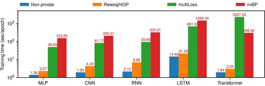
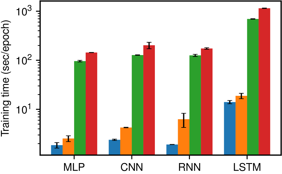
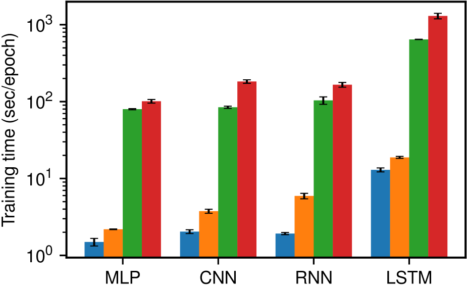
Fig. 5: Comparison of performance by varying architectures (Top: MNIST, Bottom-left: FMNIST, Bottom-right: CIFAR10, Transformer is trained on IMDB)

1. MNIST is a grayscale, image dataset of hand-written digits, consisting of 60,000 training and 10,000 test examples. Each image has $28\times 28$ pixels, and there are 10 classes (one for each digit). We trained MLP, CNN, RNN, and LSTM networks for classfication. For RNN and LSTM, we construct a sequence by considering the $i$^th row of an image as an input vector for the time step $i$. In other words, we view an image as a sequence of rows.

2. FMNIST (Fashion-MNIST) is a dataset of fashion article images designed to replace MNIST dataset. It also contains 70,000 grayscale images of size $28\times 28$ (60,000 for training and 10,000 for testing).

3. CIFAR10 is an image dataset for object classification. It consists of 50,000 training examples of $32\times 32$ RGB images. There are 10 classes, and each class has 5,000 images.

4. IMDB is a movie review dataset for binary sentiment analysis. We trained the Transformer network on this dataset using 50% of examples. The other 50% of examples were used for testing. For word embedding, rather than training from scratch, we leveraged GloVe embedding vectors of 200 dimensions, pretrained on 6 billions of tokens.

5. LSUN [49] is a large-scale scene understanding dataset, having over 59 million RGB images of size at least 256$\times$ 256, and 10 different scene categories.

6.2 Small Image Performance

We first show improvements for each architecture on the smaller image datasets (MNIST, FMNIST, CIFAR10). These datasets are not appropriate for Transformer, so we use IMDB for this architecture. Figure 5 compares the performance of the different gradient clipping computation methods on 5 different neural network models in terms of training time per epoch. For this experiment, the minibatch size $|B|$ was fixed to 32, and the models were trained for 100 epochs. As shown in the Figure 5, the proposed RewieghtGP algorithm significantly reduces the training time on all 5 different architectures. Notice that values on $y$-axis are in log scale. It is worth noting that the training of LSTM network takes significantly longer than that for other networks because the per-gradient computation must access each layer’s pre-activations and input tensor. This prevents us from using highly optimized fast implementation of LSTM such as NVIDIA’s cuDNN LSTM. For RNN, this limitation can be avoided as one can derive the gradient of loss function with respect to pre-activations from the gradient with respect to activations using the chain rule.

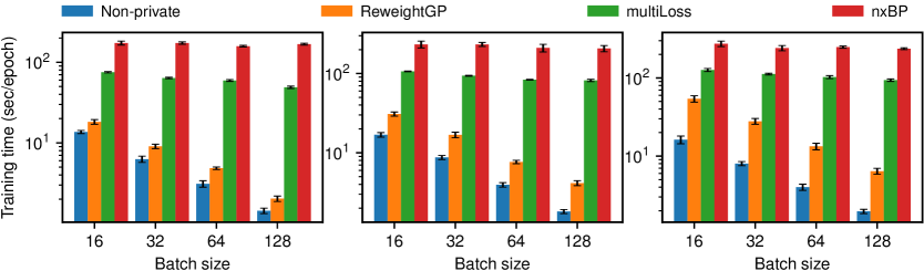
Fig. 6: Execution time by varying batch size (Left: MLP, Middle: CNN, Right: RNN)

6.3 Impact of Different Batch Size

Figure 6 shows the impact of different batch sizes on the per-epoch training time. For this experiment, we trained the MLP, CNN, and RNN models described in Section 6.1.1 on MNIST dataset by varying the batch size. The batch sizes used for training are 16, 32, 64, and 128. An interesting observation is that for Non-private and ReweightGP per-epoch training time decreases as the batch size increases, while that for nxBP remains constant regardless of batch size. This is because that both Non-private and ReweightGP can take advantage of more parallelism due to the use of larger batch. On the other hand, in nxBP computationally heavy error back-propagation happens for each training example (even if an entire batch is stored in the gpu).

6.4 Impact of Network Depth

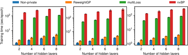
Fig. 7: Comparison of performance by varying number of hidden layers (Left: MNIST, Middle: FMNIST, Right: CIFAR10)

Before experimenting with larger and more complex architectures, we first provide network depth results for smaller architectures, as small networks are most commonly used with differential privacy [2]. We trained multiple MLP models on three datasets (MNIST, FMNIST, and CIFAR10) by using different numbers of hiddne layers: 2, 4, 6, and 8. The batch size $|B|$ is fixed to 128. As shown in Figure 7, ReweightGP algorithm significantly outperforms the naive nxBP algorithm on all three datasets. Especially on FMNIST dataset with 2 hidden layers, the proposed algorithm showed 94x speed-up over the naive nxBP algorithm.

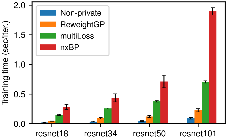
(a) ResNet (Image size: 64$\times$64)

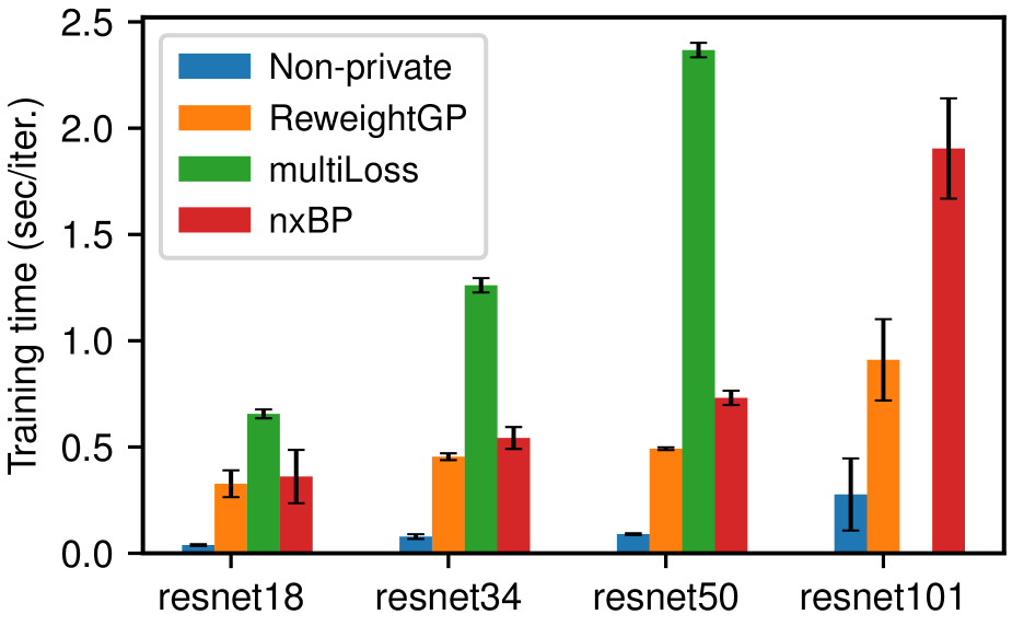
(b) ResNet (Image size: 256$\times$256)

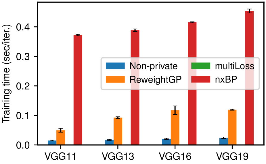
(c) VGG (Image size: 64$\times$ 64)

Fig. 8: Performance evaluation on ResNet and VGG networks. Bar for multiLoss is missing when it runs out of memory.

6.5 ResNet and VGG Networks

We now evaluate the performance on deeper architectures with millions of parameters: ResNet [19] and VGG networks [41]. For this evaluation, we froze the batchnorm parameters at values taken from pre-trained models (since batch-norm parameters do not have per-example gradients). Due to the large memory space requirement, mini-batches of size 20 are used for this experiment. Results on the LSUN dataset are shown in Figure 8. mutiLoss had out-of-memory errors on VGG networks and resnet101 for large images. We still see that ReweightGP consistently outperforms other gradient clipping algorithms (nxBP, multiLoss). The improvement is significant for images of (rescaled) size 64x64 and diminishes for size 256x256.

6.6 Image Size

Noting that image size played a key role in reducing the speedup, we investigate this further in Figure 9 using ResNet 18 with batch size 32 and image sizes ranging from 32x32 to 256x256. This causes quadratic growth in the width of the network (multiplying each dimension by c results in $c^{2}$ as many pixels) and we see that the advantage over the naive method decreases due to the extra computation per layer that ReweightGP uses.

6.7 Memory

Due to caching, it is difficult to obtain an accurate estimate of GPU memory requirements. As an alternative, we consider the largest batch size a method can support before running out of memory. For this experiment, we used ResNet 101 with 256x256 input images and varied the batch sizes. The non-private method first failed at batch size 48, ReweightGP at 36, and multiLoss at 18. nxBP operates on one example at a time (even when an entire batch is stored in the GPU). Thus we estimate the GPU memory overhead of ReweightGP compared to nonprivate to be up to $(48-36)/48\approx$ 25% for large images. At the lower end, ReweightGP with ResNet 18 with 32x32 images ran with batch size of 500 without any problems. Note nxBP under-utilizes GPU memory and parallelism (backpropagating through one example at a time). Thus, in practice, the memory overhead is manageable (i.e., allows for relatively large batch sizes) and buys us significant improvements in running time (taking better advantage of GPU parallelism).

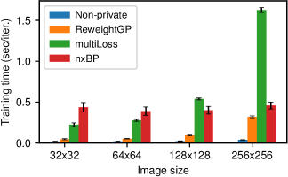
Fig. 9: Processing time by image resolution

6.8 Limitations

Overall, the experiments have shown that our proposed ReweightGP method outperforms the other methods nxBP and MultiLoss (which is often unreliable). ReweightGP requires more memory and computation per layer than nxBP. As a result, its advantage starts to decline with increased image sizes as this causes a quadratic scaling in the width of the network and consequently in the computations of ReweightGP. For very high resolution images, it may be preferable to use nxBP.

Second, some highly optimized versions of LSTM, such as the ones that use the CuDNN LSTM routines do not expose the internal gate values, so that we cannot obtain the appropriate gradients. However, less optimized versions of LSTM can be implemented in PyTorch/TensorFlow and benefit from our approach.

7 Conclusions

We presented a general framework for fast per-example gradient clipping which can be used to improve training speed under differential privacy. Prior work underutilized GPU parallelism, leading to slow training times. Our empirical evaluation showed a significant reduction in training time of differentially private models.

Per-example gradient clipping is not compatible with Batch Norm [20], but other layer normalization methods can be used instead [5, 46, 43].

References

- [1] M. Abadi, A. Agarwal, P. Barham, E. Brevdo, Z. Chen, C. Citro, G. S. Corrado, A. Davis, J. Dean, M. Devin, S. Ghemawat, I. Goodfellow, A. Harp, G. Irving, M. Isard, Y. Jia, R. Jozefowicz, L. Kaiser, M. Kudlur, J. Levenberg, D. Mané, R. Monga, S. Moore, D. Murray, C. Olah, M. Schuster, J. Shlens, B. Steiner, I. Sutskever, K. Talwar, P. Tucker, V. Vanhoucke, V. Vasudevan, F. Viégas, O. Vinyals, P. Warden, M. Wattenberg, M. Wicke, Y. Yu, and X. Zheng. TensorFlow: Large-scale machine learning on heterogeneous systems, 2015. Software available from tensorflow.org.
- [2] M. Abadi, A. Chu, I. Goodfellow, H. B. McMahan, I. Mironov, K. Talwar, and L. Zhang. Deep learning with differential privacy. In Proceedings of the 2016 ACM SIGSAC Conference on Computer and Communications Security, pages 308–318. ACM, 2016.
- [3] N. C. Abay, Y. Zhou, M. Kantarcioglu, B. M. Thuraisingham, and L. Sweeney. Privacy preserving synthetic data release using deep learning. In Machine Learning and Knowledge Discovery in Databases - European Conference, ECML PKDD 2018, Dublin, Ireland, September 10-14, 2018, Proceedings, Part I, pages 510–526, 2018.
- [4] G. Acs, L. Melis, C. Castelluccia, and E. D. Cristofaro. Differentially private mixture of generative neural networks. In ICDM, 2017.
- [5] L. J. Ba, J. R. Kiros, and G. E. Hinton. Layer normalization. CoRR, abs/1607.06450, 2016.
- [6] E. Bagdasaryan and V. Shmatikov. Differential privacy has disparate impact on model accuracy. CoRR, abs/1905.12101, 2019.
- [7] R. Bassily, A. Smith, and A. Thakurta. Private empirical risk minimization: Efficient algorithms and tight error bounds. In Proceedings of the 2014 IEEE 55th Annual Symposium on Foundations of Computer Science, FOCS ’14, pages 464–473, Washington, DC, USA, 2014. IEEE Computer Society.
- [8] B. K. Beaulieu-Jones, Z. S. Wu, C. Williams, R. Lee, S. P. Bhavnani, J. B. Byrd, and C. S. Greene. Privacy-preserving generative deep neural networks support clinical data sharing. bioRxiv, 2018.
- [9] L. Bottou. Large-scale machine learning with stochastic gradient descent. In Proceedings of COMPSTAT’2010, pages 177–186. Springer, 2010.
- [10] K. Chaudhuri, C. Monteleoni, and A. D. Sarwate. Differentially private empirical risk minimization. Journal of Machine Learning Research, 12(Mar):1069–1109, 2011.
- [11] K. Chellapilla, S. Puri, and P. Simard. High performance convolutional neural networks for document processing. In Tenth International Workshop on Frontiers in Handwriting Recognition. Suvisoft, 2006.
- [12] C. Chen, J. Lee, and D. Kifer. Renyi differentially private erm for smooth objectives. In The 22nd International Conference on Artificial Intelligence and Statistics, pages 2037–2046, 2019.
- [13] Q. Chen, C. Xiang, M. Xue, B. Li, N. Borisov, D. Kaafar, and H. Zhu. Differentially private data generative models. https://arxiv.org/pdf/1812.02274.pdf, 2018.
- [14] J. Devlin, M.-W. Chang, K. Lee, and K. Toutanova. Bert: Pre-training of deep bidirectional transformers for language understanding. In Proceedings of the 2019 Conference of the North American Chapter of the Association for Computational Linguistics: Human Language Technologies, Volume 1 (Long and Short Papers), pages 4171–4186, 2019.
- [15] C. Dwork, K. Kenthapadi, F. McSherry, I. Mironov, and M. Naor. Our data, ourselves: Privacy via distributed noise generation. In Annual International Conference on the Theory and Applications of Cryptographic Techniques, pages 486–503. Springer, 2006.
- [16] C. Dwork, F. McSherry, K. Nissim, and A. Smith. Calibrating noise to sensitivity in private data analysis. In Theory of Cryptography Conference, pages 265–284. Springer, 2006.
- [17] I. Goodfellow. Efficient per-example gradient computations. arXiv preprint arXiv:1510.01799, 2015.
- [18] I. J. Goodfellow, Y. Bengio, and A. Courville. Deep Learning. MIT Press, Cambridge, MA, USA, 2016. http://www.deeplearningbook.org.
- [19] K. He, X. Zhang, S. Ren, and J. Sun. Deep residual learning for image recognition. In CVPR, 2016.
- [20] S. Ioffe and C. Szegedy. Batch normalization: Accelerating deep network training by reducing internal covariate shift. CoRR, abs/1502.03167, 2015.
- [21] R. Iyengar, J. P. Near, D. Song, O. Thakkar, A. Thakurta, and L. Wang. Towards practical differentially private convex optimization. In Towards Practical Differentially Private Convex Optimization, page 0. IEEE.
- [22] Y. Jia. Learning semantic image representations at a large scale. PhD thesis, UC Berkeley, 2014.
- [23] J. Jordon, J. Yoon, and M. van der Schaar. Pate-gan: Generating synthetic data with differential privacy guarantees. In ICLR, 2019.
- [24] D. Kifer, A. Smith, and A. Thakurta. Private convex empirical risk minimization and high-dimensional regression. In Conference on Learning Theory, pages 25–1, 2012.
- [25] D. Kingma and J. Ba. Adam: A method for stochastic optimization. International Conference on Learning Representations, 12 2014.
- [26] J. Lee and D. Kifer. Concentrated differentially private gradient descent with adaptive per-iteration privacy budget. In Proceedings of the 24th ACM SIGKDD International Conference on Knowledge Discovery & Data Mining, 2018.
- [27] H. B. McMahan, G. Andrew, U. Erlingsson, S. Chien, I. Mironov, N. Papernot, and P. Kairouz. A general approach to adding differential privacy to iterative training procedures. arXiv preprint arXiv:1812.06210, 2018.
- [28] H. B. McMahan, D. Ramage, K. Talwar, and L. Zhang. Learning differentially private recurrent language models. In International Conference on Learning Representations, 2018.
- [29] I. Mironov. Renyi differential privacy. In Computer Security Foundations Symposium (CSF), 2017 IEEE 30th, pages 263–275. IEEE, 2017.
- [30] N. Papernot, M. Abadi, Úlfar Erlingsson, I. Goodfellow, and K. Talwar. Semi-supervised knowledge transfer for deep learning from private training data. In Proceedings of the International Conference on Learning Representations, 2017.
- [31] N. Papernot, S. Chien, C. C. Choo, G. M. Andrew, and I. Mironov. TensorFlow Privacy.
- [32] N. Papernot, S. Song, I. Mironov, A. Raghunathan, K. Talwar, and Úlfar Erlingsson. Scalable private learning with pate. In International Conference on Learning Representations (ICLR), 2018.
- [33] A. Paszke, S. Gross, S. Chintala, G. Chanan, E. Yang, Z. DeVito, Z. Lin, A. Desmaison, L. Antiga, and A. Lerer. Automatic differentiation in PyTorch. In NeurIPS Autodiff Workshop, 2017.
- [34] N. Phan, Y. Wang, X. Wu, and D. Dou. Differential privacy preservation for deep auto-encoders: an application of human behavior prediction. In AAAI, 2016.
- [35] M. Reimherr and J. Awan. KNG: the k-norm gradient mechanism. In NeurIPS, 2019.
- [36] H. Robbins and S. Monro. A stochastic approximation method. The annals of mathematical statistics, pages 400–407, 1951.
- [37] G. Rochette, A. Manoel, and E. W. Tramel. Efficient per-example gradient computations in convolutional neural networks. ArXiv, abs/1912.06015, 2019.
- [38] S. Ruder. An overview of gradient descent optimization algorithms. CoRR, abs/1609.04747, 2016.
- [39] R. Shokri and V. Shmatikov. Privacy-preserving deep learning. In Proceedings of the 22Nd ACM SIGSAC Conference on Computer and Communications Security, 2015.
- [40] R. Shokri, M. Stronati, C. Song, and V. Shmatikov. Membership inference attacks against machine learning models. In IEEE Symposium on Security and Privacy (SP), 2017.
- [41] K. Simonyan and A. Zisserman. Very deep convolutional networks for large-scale image recognition. In International Conference on Learning Representations, 2015.
- [42] O. Thakkar, G. Andrew, and H. B. McMahan. Differentially private learning with adaptive clipping. CoRR, abs/1905.03871, 2019.
- [43] D. Ulyanov, A. Vedaldi, and V. S. Lempitsky. Instance normalization: The missing ingredient for fast stylization. CoRR, abs/1607.08022, 2016.
- [44] A. Vaswani, N. Shazeer, N. Parmar, J. Uszkoreit, L. Jones, A. N. Gomez, Ł. Kaiser, and I. Polosukhin. Attention is all you need. In Advances in neural information processing systems, pages 5998–6008, 2017.
- [45] D. Wang, M. Ye, and J. Xu. Differentially private empirical risk minimization revisited: Faster and more general. In Advances in Neural Information Processing Systems 30, pages 2719–2728. Curran Associates, Inc., 2017.
- [46] Y. Wu and K. He. Group normalization. In ECCV, 2018.
- [47] L. Xie, K. Lin, S. Wang, F. Wang, and J. Zhou. Differentially private generative adversarial network, 2018.
- [48] Z. Yang, Z. Dai, Y. Yang, J. Carbonell, R. Salakhutdinov, and Q. V. Le. Xlnet: Generalized autoregressive pretraining for language understanding. arXiv preprint arXiv:1906.08237, 2019.
- [49] F. Yu, Y. Zhang, S. Song, A. Seff, and J. Xiao. Lsun: Construction of a large-scale image dataset using deep learning with humans in the loop. ArXiv, abs/1506.03365, 2015.
- [50] L. Yu, L. Liu, C. Pu, M. E. Gursoy, and S. Truex. Differentially private model publishing for deep learning. 2019 IEEE Symposium on Security and Privacy (SP), pages 332–349, 2019.
- [51] J. Zhang, K. Zheng, W. Mou, and L. Wang. Efficient private erm for smooth objectives. In Proceedings of the 26th International Joint Conference on Artificial Intelligence, pages 3922–3928. AAAI Press, 2017.