1 Introduction

Crystal plasticity and dislocations are a fundamental theme in the mechanics of solids. Whereas the calculus of variations has been very helpful in the study of nonlinear elasticity and phase transitions, the study of plasticity and dislocations has proven much more demanding. Dislocations are topological singularities of the strain field, which share many features with other important classes of topological defects, such as Ginzburg-Landau vortices, defects in liquid crystals, harmonic maps, models of superconductivity. Their importance for the understanding of the yield behavior of crystals motivated a large interest, and indeed in the last decade tools have been developed to study individual dislocations, both in reduced two-dimensional formulations in which one deals with point singularities [Pon07, ACP11, DGP12], and, with some geometrical restrictions, in the three dimensional setting in which singularities are lines [CGO15]. In this paper we go beyond the scale of single dislocation lines and derive macroscopic strain-gradient plasticity, starting from a Peierls-Nabarro model. The limiting model combines effects at different scales, it includes both long-range interactions of singularities and a short-range strain-gradient term which arises from the self-interaction of dislocations. This result does not require any restriction on the admissible configurations of defects. One important tool is a self-similar multiscale decomposition of the interaction kernel.

In order to relate the presence of dislocations to macroscopic plastic deformations of solids, in particular within the framework of a strain-gradient theory of plasticity, one needs to consider the situation in which many dislocations are present and their density couples to macroscopic deformation of the material. This scaling was first addressed in the context of Ginzburg-Landau vortices by Sandier and Serfaty [SS03]. For point dislocations in two dimensions this regime was first studied in [GLP10] in a dilute geometrically linear setting, and then generalized to geometrically nonlinear models [MSZ14, MSZ15] and to the non-dilute setting [Gin19a, Gin19b]. A model based on microrotations was presented and studied in two dimensions in [LL16], where in particular the Read-Shockley formula for the energy of small-angle grain boundaries, based on the appearence of an array of point dislocations, was derived.

The three-dimensional case is substantially more subtle. Firstly, because the geometry plays an important role in the interaction between line singularities, and secondly, because it is a higher-order tensorial problem, in which the energy only controls some components of the relevant strain field. Moreover, the anisotropy of the energy leads to additional relaxation at intermediate scales [CG09, CGM11, CGO15].

A natural geometrical restriction involves assuming that a single slip plane is active, so that the singularities are lines in a prescribed plane. The elastic problem can then be solved (implicitly) and results in a nonlocal interaction between the singularities, which scales as the $H^{1/2}$ norm of the slip field. This model, which is in the spirit of the classical Peierls-Nabarro model, was proposed and studied numerically in [Ort99, KCO02, KO04], in a regime in which a few individual dislocations are present. In the same regime, a scalar simplification of the model was studied analytically in [GM05, GM06]. In the limit of small lattice spacing ${\varepsilon}$, the energy concentrates along the dislocations and the problem reduces to a line-tension model; the relevant independent variable is a measure concentrated on a line. One important tool was the study of variational convergence for phase transitions with nonlocal interactions, see also [ABS94, ABS98, FG07, SV12]. The extension to the physically relevant vectorial situation in [CG09, CGM11] lead to the discovery of unexpected microstructures at intermediate scales, which arise due to the interplay of the localized nature of the singularity with the anisotropy of the vectorial elastic energy. A generalization to multiple planes is discussed in [CG15].

We address here a scaling regime in which the total length of the dislocations diverges, rendering the average line-tension energy comparable with the macroscopic long-range elastic energy. This is a natural scaling in the presence of topological singularities, since it balances the long-range interaction with the short-range core energies. This critical scaling regime was first considered in the context of Ginzburg-Landau vortices and models of superconductivity [SS03, SS07, BJOS12, BJOS13]. Whereas some ideas are closely related, the vectorial and anisotropic nature of the dislocation problem renders a direct transfer difficult and requires new techniques, in particular for treating the microstructures at intermediate scales.

We derive here a macroscopic strain-gradient theory, where the macroscopic effect of the dislocations is captured by a dislocation density, which is a measure in $H^{-1/2}$. The mechanical implications of this result and the connection to strain-gradient theories of plasticity have been discussed in [CGM16, ACGO18]. These include dislocation microstructures at intermediate scales, in the form of dislocation networks, the study of which has long been an important problem in mechanics [HL68, FH93, OR99, GA05, GGK07, Ach10, GGI10, Ber16, MSZ16]. We present here a joint convergence result, in which the two terms are derived in one step from the Peierls-Nabarro model in the limit of small lattice spacing. The study of a single limiting process is crucial to obtain the limiting behavior of both the local and the nonlocal term; if the various homogenization and relaxation steps are taken separately then the nonlocal (interaction) term disappears [CGM17].

The main difficulty in the proof is to obtain a joint treatment of the many different scales present in the problem. The discrete nature of the dislocations leads to localization and to slip fields in $BV(\Omega;\mathbb{Z}^{N})$, at the same time the nonlocal part requires slip fields in $H^{1/2}{(\Omega;\mathbb{R}^{N})}$. These two spaces are, except for constants, disjoint (see Lemma 3.2 below), hence both requirements can only be realized approximately. This is performed introducing a number of well-separated scales, regularizations and cutoffs, as discussed in the introduction to Section 5 for the upper bound and Section 6 for the lower bound. Indeed, both the original functional and the limiting functional are finite on $H^{1/2}{(\Omega;\mathbb{R}^{N})}$, whereas the relaxation steps occur at intermediate scales, where the relevant functions belong to $BV(\Omega;\mathbb{Z}^{N})$. As it is clear from this summary, our argument makes a strong usage of the existence of a lifting of the dislocation density to a function of bounded variation. The extension to the unconstrained three-dimensional case will probably require a different functional framework, which could possibly be formulated via cartesian currents [Hoc13, CGM15, SvG16].

We now formulate the model we study. The total energy associated to a phase field $u\in L^{2}(\Omega;\mathbb{R}^{N})$, with $\Omega\subset\mathbb{R}^{2}$ open and bounded, is

$$E_{\varepsilon}[u,\Omega]:= \frac{1}{{\varepsilon}}\int_{\Omega}W(u(x))dx$$

$$+\int_{\Omega\times\Omega}\Gamma(x-y)(u(x)-u(y))\cdot(u(x)-u(y))dxdy.$$ (1.1)

The nonlinear potential $W:\mathbb{R}^{N}\to[0,\infty)$ satisfies

$$\frac{1}{c}\,{\mathrm{dist}}^{2}(\xi,\mathbb{Z}^{N})\leq W(\xi)\leq c\,{\mathrm{dist}}^{2}(\xi,\mathbb{Z}^{N})$$ (1.2)

for some $c>0$. The elasticity kernel $\Gamma\in L^{1}_{\mathrm{loc}}(\mathbb{R}^{2};\mathbb{R}^{N\times N}_{\mathrm{sym}})$ is defined by

$$\Gamma(z):=\frac{1}{|z|^{3}}\hat{\Gamma}\left(\frac{z}{|z|}\right)\,,$$ (1.3)

where $\mathbb{R}^{N\times N}_{\mathrm{sym}}$ denotes the set of symmetric $N\times N$ matrices and $\hat{\Gamma}\in L^{\infty}(S^{1};\mathbb{R}^{N\times N}_{\mathrm{sym}})$ obeys, for some $c>0$,

$$\hat{\Gamma}(z)=\hat{\Gamma}(-z)\text{ and }\frac{1}{c}|\xi|^{2}\leq\hat{\Gamma}(z)\xi\cdot\xi\leq c|\xi|^{2}\hskip 14.22636pt\text{ for all }\xi\in\mathbb{R}^{N},\,z\in S^{1}\,.$$ (1.4)

The specific form of $\hat{\Gamma}$ depends on the elastic constants and the Burgers vectors of the crystal, for example for an elastically isotropic cubic crystal one obtains $\Gamma=\Gamma^{\mathrm{cubic}}$, where

$$\Gamma^{\mathrm{cubic}}(z):=\frac{\mu}{16\pi(1-\overline{\nu})|z|^{3}}\left(\begin{matrix}\overline{\nu}+1-3\overline{\nu}\frac{z_{2}^{2}}{|z|^{2}}&3\overline{\nu}\frac{z_{1}z_{2}}{|z|^{2}}\\ 3\overline{\nu}\frac{z_{1}z_{2}}{|z|^{2}}&\overline{\nu}+1-3\overline{\nu}\frac{z_{1}^{2}}{|z|^{2}}\end{matrix}\right)\,.$$ (1.5)

In (1.5) $\overline{\nu}$ and $\mu$ denote the material’s Poisson’s ratio and shear modulus, respectively (see [CG09]). It is easy to see that for $\mu>0$ and $\overline{\nu}\in(-1,1/2)$ the kernel $\Gamma^{\mathrm{cubic}}$ fulfills the assumption (1.4).

In order to present our main result we first introduce the several effective energy densities which are generated by the rescaling procedure. Detailed explanations on the physical significance of the different steps are given in Section 2. In a first step the nonlocal kernel $\Gamma$ generates an unrelaxed line-tension energy $\psi:\mathbb{Z}^{N}\times S^{1}\to{[0,\infty)}$ by

$$\psi(b,n):=2\int_{\{x\cdot n=1\}}\Gamma(x)b\cdot b\,d\mathcal{H}^{1}(x).$$ (1.6)

Relaxation at the line-tension scale leads to the $BV$-elliptic envelope $\psi_{\mathrm{rel}}:\mathbb{Z}^{N}\times S^{1}\to[0,\infty)$ of $\psi:\mathbb{Z}^{N}\times S^{1}\to[0,\infty)$, defined by

$$\begin{split}\psi_{\mathrm{rel}}(b,n):=&\inf\Bigl{\{}\frac{1}{2}\int_{J_{u}\cap B_{1}}\psi([u],\nu)d\mathcal{H}^{1}:u\in BV_{\mathrm{loc}}(\mathbb{R}^{2};\mathbb{Z}^{N}),\\ &\hskip 42.67912pt\mathop{\mathrm{supp}}(u-u^{0}_{b,n})\subset\subset B_{1}\Bigr{\}},\end{split}$$ (1.7)

where $u^{0}_{b,n}(x):=b\chi_{\{x\cdot n>0\}}$ and $\nu$ is the normal to the jump set $J_{u}$ of $u$. We recall that the concept of $BV$-elliptic envelope was introduced and studied in [AB90a, AB90b], see also [AFP00, Sect. 5.3].

Finally, in the second relaxation step one obtains a continuous energy density $g:\mathbb{R}^{N\times 2}\to{[0,\infty)}$ defined as the convex envelope of

$$g_{0}(A):=\begin{cases}0,&\text{ if }A=0,\\ \psi_{\mathrm{rel}}(b,n),&\text{ if }A=b\otimes n\text{ for }b\in\mathbb{Z}^{N},n\in S^{1},\\ \infty,&\text{ otherwise.}\end{cases}$$ (1.8)

In particular, the function $g$ turns out to be positively 1-homogeneous, see [CGM17].

Our main result is the following.

Theorem 1.1.

Let $\Omega\subset\mathbb{R}^{2}$ be a bounded connected Lipschitz domain, and let $E_{\varepsilon}[\cdot,\Omega]$ be defined as in (1.1), with $W$ and $\Gamma$ which satisfy (1.2)–(1.4).

We say that a family of functions $u_{\varepsilon}\in L^{2}(\Omega;\mathbb{R}^{N})$, ${\varepsilon}>0$, converges to $u$ if

$$\frac{u_{\varepsilon}}{\ln(1/{\varepsilon})}\to u\hskip 28.45274pt\text{ in }L^{2}(\Omega;\mathbb{R}^{N})\hskip 28.45274pt\text{ as }{\varepsilon}\to 0.$$ (1.9)

With respect to this convergence we have

$$\Gamma\hbox{-}\lim_{\varepsilon\to 0}\frac{1}{(\ln(1/\varepsilon))^{2}}E_{\varepsilon}[\cdot,\Omega]=F_{0}[\cdot,\Omega]\,,$$

where $F_{0}$ is defined by

$$F_{0}[u,\Omega]:=F_{\mathrm{\mathrm{self}}}[u,\Omega]+\int_{\Omega\times\Omega}\Gamma(x-y)(u(x)-u(y))\cdot(u(x)-u(y))dxdy$$ (1.10)

and

$$F_{\mathrm{\mathrm{self}}}[u,\Omega]:=\int_{\Omega}g(\nabla u)dx+\int_{\Omega}g\left(\frac{dD^{s}u}{d|D^{s}u|}\right)d|D^{s}u|$$ (1.11)

if $u\in BV(\Omega;\mathbb{R}^{N})\cap H^{1/2}(\Omega;\mathbb{R}^{N})$, and $F_{0}[u,\Omega]=\infty$ otherwise. Here $g:\mathbb{R}^{N\times 2}\to[0,\infty)$ is the convex envelope of the function $g_{0}$ defined from the kernel $\Gamma$ in (1.6)–(1.8).

Further, the functionals $(\ln(1/{\varepsilon}))^{-2}E_{\varepsilon}[\cdot,\Omega]$ are, with respect to the stated convergence, equicoercive, in the sense that if $u_{\varepsilon}\in L^{2}(\Omega;\mathbb{R}^{N})$ are such that $E_{\varepsilon}[u_{\varepsilon},\Omega]\leq C(\ln(1/{\varepsilon}))^{2}$ for all ${\varepsilon}$ then there is a subsequence ${\varepsilon}_{k}\to 0$ such that, for some $d_{k}\in\mathbb{Z}^{N}$ and some $u\in L^{2}(\Omega;\mathbb{R}^{N})$, one has

$$\lim_{k\to\infty}\frac{u_{{\varepsilon}_{k}}-d_{k}}{\ln(1/{\varepsilon}_{k})}=u\hskip 28.45274pt\text{ in }L^{2}(\Omega;\mathbb{R}^{N}).$$ (1.12)

We remark that $\psi_{\mathrm{rel}}$ coincides with the line-tension energy density obtained in the subcritical regime [CGM11], see Theorem 2.1 below.

The proof of above theorem is a combination of various results proved in the rest of the paper. The compactness assertion follows from Proposition 3.1 in Section 3, the upper bound from Proposition 5.2 in Section 5, and the lower bound from Proposition 6.1 in Section 6.

In closing this Introduction we briefly recall the connection between $E_{\varepsilon}$ and the classical Peierls-Nabarro model which contains the elastic energy over a three-dimensional domain. The Peierls-Nabarro model, as generalized in [Ort99, KCO02, KO04] to three dimensions, expresses the free energy in terms of the slip $v:\Omega\to\mathbb{R}^{3}$ as

$$E_{\rm free}[v]:=E_{\rm elastic}[v]+E_{\rm interfacial}[v]\,.$$

Here the first term represents the long-range elastic distortion due to the slip and the second term penalizes slips that are not integer multiples of the Burgers vectors of the crystal lattice. One denotes by ${b}_{1}$, …, ${b}_{N}$ the relevant Burgers vectors and considers slips of the form

$$v=u_{1}{b}_{1}+...+u_{N}{b}_{N}$$

where $u:\Omega\subset\mathbb{R}^{2}\to\mathbb{R}^{N}$. The term $E_{\rm interfacial}$ penalizes values of $u$ far from $\mathbb{Z}^{N}$, so that $v$ is close to the lattice generated by $\{b_{1},\dots,b_{N}\}$. A simple model is

$$E_{\rm interfacial}[v]=\frac{1}{{\varepsilon}}\int_{\Omega}{\mathrm{dist}}^{2}(u,\mathbb{Z}^{N})dx,$$

where $u$ is related to $v$ as stated above. We observe that the specific functional form does not contribute to the limit. At variance with many classical results in $\Gamma$-convergence for phase-field models of phase transitions there is no equipartition of energy, and the only role of the interfacial energy is to force $u$ to jump on a scale ${\varepsilon}$. The limiting energy arises then completely from the elastic term, as it is apparent from the characterization of $g$ and $\psi$ in terms of the kernel $\Gamma$ in (1.6)–(1.8).

The elastic interaction is given by

$$E_{\rm elastic}[v]=\inf\left\{\int_{\Omega\times\mathbb{R}}\frac{1}{2}\mathbb{C}\nabla U\cdot\nabla U\,dx\right\},$$

where the displacement $U:\Omega\times\mathbb{R}\to\mathbb{R}^{3}$ is required to have a discontinuity of $v=\sum u_{i}b_{i}$ across $\Omega\times\{x_{3}=0\}$. Minimizing out $U$ leads to a nonlocal functional of $u$ of the kind of (1.1) up to boundary effects which do not influence the leading-order behavior, see [GM05, GM06] for a discussion. The factor ${\varepsilon}$ in $E_{\rm interfacial}$ is proportional to the lattice spacing and arises from the different scaling of the bulk and the interfacial term. We refer to [GM05, CGM16] for a more detailed discussion of this relation.

Remark 1.2.

We discuss in this paper the case that $\Omega$ is a bounded Lipschitz set. Similar results can be obtained, with the same proofs, for the case that $\Omega$ is a torus. In the latter case it is easy to see that the elastic energy $E_{\rm elastic}$ coincides with the nonlocal energy in $E_{\varepsilon}$, up to lower-order terms which are continuous in the topology considered here. This leads to the model described in [CGM16].

2 Limits at separated scales

In this section we briefly review two previous results on different scalings which have been mentioned in the introduction and that will be used in the proofs.

If a sequence $u_{\varepsilon}$ has energy proportional to $\ln(1/{\varepsilon})$, in the sense that $E_{\varepsilon}[u_{\varepsilon},\Omega]\leq C\ln(1/{\varepsilon})$, then asymptotically $u_{\varepsilon}$ describes dislocations with finite total length, and the limiting energy is given by an integral over the line. This is called the line-tension approximation and was studied in [GM05, CGM11].

Theorem 2.1 ([CGM11, Th. 1.1]).

Let $\Omega\subset\mathbb{R}^{2}$ be a bounded connected Lipschitz domain, and let $E_{\varepsilon}[\cdot,\Omega]$ be defined as in (1.1), with $W$ and $\Gamma$ which satisfy (1.2)–(1.4).

The functionals $1/(\ln(1/\varepsilon))E_{\varepsilon}[\cdot,\Omega]$ are $L^{1}$-equicoercive, in the sense that if $E_{\varepsilon}[u_{\varepsilon},\Omega]\leq C\ln(1/\varepsilon)$ then there are $d_{\varepsilon}\in\mathbb{Z}^{N}$ and $u\in BV(\Omega;\mathbb{Z}^{N})$ such that $u_{\varepsilon}-d_{\varepsilon}$ has a subsequence that converges to $u$ in $L^{1}(\Omega;\mathbb{R}^{N})$.

Further, we have

$$\Gamma\hbox{-}\lim_{\varepsilon\to 0}\frac{1}{\ln(1/\varepsilon)}E_{\varepsilon}[\cdot,\Omega]=E^{\mathrm{LT,rel}}[\cdot,\Omega]\,,$$

with respect to strong $L^{1}$ convergence, where the relaxed line-tension fuctional $E^{\mathrm{LT,rel}}$ is defined by

$$E^{\mathrm{LT,rel}}[u,\Omega]:=\begin{cases}\displaystyle\int_{J_{u}\cap\Omega}\psi_{\mathrm{rel}}\left([u],\nu\right)d\mathcal{H}^{1},&\text{ if }u\in SBV(\Omega;\mathbb{Z}^{N}),\\ \infty,&\text{ otherwise,}\end{cases}$$ (2.1)

with $\psi_{\mathrm{rel}}$ obtained from $\Gamma$ as in (1.6) and (1.7).

In (2.1) and in the rest of this paper we use standard notation on functions of bounded variations, which we now briefly recall. The elements of $BV(\Omega;\mathbb{R}^{N})$, $\Omega\subset\mathbb{R}^{2}$, are the functions in $L^{1}(\Omega;\mathbb{R}^{N})$ whose distributional derivative $Du$ is a bounded measure on $\Omega$ ($D^{s}u$ denotes the part of this measure which is singular with respect to the Lebesgue measure). In turn, $SBV(\Omega;\mathbb{R}^{N})$ denotes the space of special functions of bounded variation, which are the functions in $BV(\Omega;\mathbb{R}^{N})$ whose distributional gradient can be characterized as $Du=\nabla u\mathcal{L}^{2}+[u]\otimes\nu\mathcal{H}^{1}{\mathchoice{\,\hbox{\vrule width=0.2pt\vbox to7.0pt{\vfill\hrule width=7.0pt,height=0.2pt}}\,}{\,\hbox{\vrule width=0.2pt\vbox to7.0pt{\vfill\hrule width=7.0pt,height=0.2pt}}\,}{\,\hbox{\vrule width=0.2pt\vbox to5.0pt{\vfill\hrule width=5.0pt,height=0.2pt}}\,}{\,\hbox{\vrule width=0.2pt\vbox to3.35pt{\vfill\hrule width=3.35pt,height=0.2pt}}\,}}J_{u}$. Here $J_{u}$ is a 1-rectifiable set called the jump set of $u$, and it is defined as the set of points for which $u$ does not have an approximate limit. The normal to this set is denoted by $\nu$, and $[u]=u^{+}-u^{-}$ denotes the jump of the function $u$ across the set $J_{u}$. For any $\mathcal{H}^{1}$-a.e. $x\in J_{u}$ one has

$$\lim_{r\to 0}\frac{\mathcal{H}^{1}(J_{u}\cap B_{r}(x))}{2r}=1$$

and

$$\lim_{r\to 0}\frac{1}{r^{2}}\int_{B_{r}(x)\cap\{\pm(y-x)\cdot\nu>0\}}|u-u^{\pm}(x)|dy=0.$$

We refer to [AFP00] for details.

The main difficulty in the proof of Theorem 2.1 is the fact that this problem has no natural rescaling, since infinitely many scales asymptotically contribute to the energy. The proof is based on a dyadic decomposition of the interaction kernel, which is also used in Section 6 below, and on an iterative mollification technique which permits to show that microstructure can only appear at few scales, and therefore that on the average scale there is no microstructure. This permits to pass from the nonlocal functional $E_{\varepsilon}$ to a line-tension functional with the unrelaxed energy $\psi$; the relaxation from $\psi$ to $\psi_{\mathrm{rel}}$ takes then place at the line-tension level and does not couple to the nonlocality of $E_{\varepsilon}$. We refer to [CGM11] for details and we remark that a similar formula for the subcritical regime also holds without the geometric restriction to a single plane, if the dislocations are dilute [CGO15].

For later reference we observe that (1.4) and the definition in (1.6) imply that $c|b|\leq\psi(b,n)$ for all $b\in\mathbb{Z}^{N}$, $n\in S^{1}$, and by (1.7) we obtain with Jensen’s inequality

$$c|b|\leq\psi_{\mathrm{rel}}(b,n)\leq\psi(b,n)\hskip 14.22636pt\text{ for all $b\in\mathbb{Z}^{N}$, $n\in S^{1}$}.$$ (2.2)

The transition from scaled line-tension functionals to a functional with a continuous distribution of dislocations was studied in [CGM17]. Here two effects are present. Firstly, by the rescaling the discrete nature of the dislocations is lost, and macroscopically one only sees the effective dislocation density, passing from $\psi_{\mathrm{rel}}$ to $g_{0}$. This corresponds to recovering continuous slips from superposition of many atomic-scale plastic slips, and naturally relates to strain-gradient plasticity models. Secondly, and already at the macroscopic scale, one relaxes $g_{0}$ (which is finite only on certain rank-one matrices) to the macrosopic energy $g$. As usual in problems with linear growth, the gradient constraint does not affect the effective energy density which turns out to be convex, see [KK16] for a general statement.

Theorem 2.2.

Let $\Omega\subset\mathbb{R}^{2}$ be a bounded connected Lipschitz domain, and let $\psi:\mathbb{Z}^{N}\times S^{1}\to[0,\infty)$ obey $\frac{1}{c}|b|\leq\psi(b,n)$ for all $b\in\mathbb{Z}^{N}$ and $n\in S^{1}$. The functionals

$$E^{\mathrm{LT}}_{\sigma}[u,\Omega]:=\begin{cases}\displaystyle\int_{J_{u}\cap\Omega}\sigma\psi\left(\frac{[u]}{\sigma},\nu\right)d\mathcal{H}^{1},&\text{ if }u\in SBV(\Omega;\sigma\mathbb{Z}^{N}),\\ \infty,&\text{ otherwise,}\end{cases}$$ (2.3)

are equicoercive with respect to the strong $L^{1}$ topology, in the sense that if $\sigma_{k}>0$, $\sigma_{k}\to 0$ and $E^{\mathrm{LT}}_{\sigma_{k}}[u_{k},\Omega]\leq C$ then there are $d_{k}\in\mathbb{R}^{N}$ and $u\in BV(\Omega;\mathbb{R}^{N})$ such that $u_{k}-d_{k}$ has a subsequence that converges to $u$ in $L^{1}(\Omega;\mathbb{R}^{N})$.

Further, with respect to this topology,

$$\Gamma\hbox{-}\lim_{\sigma\to 0}E^{\mathrm{LT}}_{\sigma}[\cdot,\Omega]=E^{\mathrm{LT}}_{0}[\cdot,\Omega],$$

where

$$E^{\mathrm{LT}}_{0}[u,\Omega]:=\begin{cases}\displaystyle\int_{\Omega}g\left(\frac{dDu}{d|Du|}\right)d|Du|,&\text{ if }u\in BV(\Omega;\mathbb{R}^{N}),\\ \infty,&\text{ otherwise.}\end{cases}$$ (2.4)

The function $g$ is positively 1-homogeneous, obeys $\frac{1}{c}|A|\leq g(A)\leq c|A|$, and coincides with the convex envelope of $g_{0}$, which is defined from $\psi$ via $\psi_{\mathrm{rel}}$ as in (1.7) and (1.8).

We observe that in [CGM17, Eq. (1.4)] there is a typo, the integral should be (as in (2.4) above) over $\Omega$, not $J_{u}$.

Proof.

This statement reduces to [CGM17, Theorem 1.1] in the case that $\psi$ is $BV$-elliptic (i.e., if $\psi=\psi_{\mathrm{rel}}$), after a change in notation.

In the general case we observe that for any (fixed) $\sigma>0$ by [CGM15] the functional

$$E^{\mathrm{LT,rel}}_{\sigma}[u,\Omega]:=\begin{cases}\displaystyle\int_{J_{u}\cap\Omega}\sigma\psi_{\mathrm{rel}}\left(\frac{[u]}{\sigma},\nu\right)d\mathcal{H}^{1},&\text{ if }u\in SBV(\Omega;\sigma\mathbb{Z}^{N}),\\ \infty,&\text{ otherwise,}\end{cases}$$ (2.5)

is the relaxation of $E^{\mathrm{LT}}_{\sigma}$, and that $\psi_{\mathrm{rel}}$ is $BV$-elliptic and has linear growth, in the sense that

$$\frac{1}{c}|b|\leq\psi_{\mathrm{rel}}(b,n)\leq c|b|\hskip 14.22636pt\text{ for all }b\in\mathbb{Z}^{N},n\in S^{1}.$$

Therefore the $\Gamma$-limit of the sequence $E^{\mathrm{LT}}_{\sigma}$ is the same as the $\Gamma$-limit of the sequence $E^{\mathrm{LT,rel}}_{\sigma}$, we refer to [Dal93, Prop. 6.11] for details.

Finally, as mentioned above [CGM17, Theorem 1.1] implies that the sequence $E^{\mathrm{LT,rel}}_{\sigma}$ $\Gamma$-converges to $E^{\mathrm{LT}}_{0}$. Coercivity is also inherited, since $\psi_{\mathrm{rel}}\leq\psi$. This concludes the proof. ∎

In proving our main result we shall have to take into account both these results, but also include the effects of the long-range elastic energy, which scales as the squared $H^{1/2}$ norm of $u$. We remark that $H^{1/2}$ is singular with respect to the natural spaces of piecewise constant functions entering the above results, hence one cannot recover Theorem 1.1 from a direct combination of Theorem 2.1 and Theorem 2.2.

3 Compactness

The functions $u_{\varepsilon}/\ln(1/\varepsilon)$ belong to the space $H^{1/2}(\Omega;\mathbb{R}^{N})$, the limit however will belong also to $BV(\Omega;\mathbb{R}^{N})$. The key step in the proof of the compactness result is to produce a new sequence of functions, called $v_{\varepsilon}$ in the proof below, which belong to $BV(\Omega;\mathbb{Z}^{N})$ and are close to $u_{\varepsilon}$.

Proposition 3.1 (Compactness).

Let $\Omega\subset\mathbb{R}^{2}$ be a bounded connected Lipschitz domain, and let $E_{\varepsilon}[\cdot,\Omega]$ be defined as in (1.1), with $W$ and $\Gamma$ which satisfy (1.2)–(1.4).

Let $u_{\varepsilon}$ be a family with $E_{\varepsilon}[u_{\varepsilon},\Omega]\leq M(\ln(1/{\varepsilon}))^{2}$ for some $M>0$. Then there are a function $u\in BV(\Omega;\mathbb{R}^{N})\cap H^{1/2}(\Omega;\mathbb{R}^{N})$, vectors $d_{\varepsilon}\in\mathbb{Z}^{N}$ and a subsequence ${\varepsilon}_{k}\to 0$ such that

$$\frac{1}{\ln(1/{{\varepsilon}_{k}})}(u_{{\varepsilon}_{k}}-d_{{\varepsilon}_{k}})\to u\hskip 14.22636pt\text{ in $L^{2}(\Omega;\mathbb{R}^{N})$.}$$ (3.1)

Before starting the proof we recall the basic definition and some properties of the space $H^{1/2}$. We define the homogeneous $H^{1/2}$ seminorm of a measurable function $f:\Omega\to\mathbb{R}$, for an open set $\Omega\subset\mathbb{R}^{2}$, by

$$[f]_{H^{1/2}(\Omega)}^{2}:=\int_{\Omega\times\Omega}\frac{|f(x)-f(y)|^{2}}{|x-y|^{3}}dxdy.$$ (3.2)

We observe that if $\Omega$ is bounded then for any $f$ there is $a_{f}\in\mathbb{R}$ such that

$$\|f-a_{f}\|_{L^{2}(\Omega)}\leq c_{\Omega}[f]_{H^{1/2}(\Omega)}.$$

This can be proven directly from the definition of $[f]_{H^{1/2}(\Omega)}$, letting $a_{f}$ be the average of $f$ over $\Omega$. If $\Omega$ is bounded and Lipschitz, then any sequence $f_{j}$ which converges weakly in $L^{2}$ and is bounded in the $H^{1/2}$ seminorm converges strongly in $L^{2}$, see for example [DNPV12, Section 7]. One can see that this norm is equivalent the one obtained by the trace method.

We next recall that $BV(\Omega;\mathbb{Z}^{N})$ is (up to constants) disjoint from $H^{1/2}(\Omega;\mathbb{R}^{N})$, which only contains functions that “do not jump”. This fact is made precise by the following Lemma.

Lemma 3.2.

Let $\Omega\subset\mathbb{R}^{2}$ be open, $u\in BV(\Omega)\cap H^{1/2}(\Omega)$. Then $\mathcal{H}^{1}(J_{u})=0$.

In particular, if $u\in BV(\Omega;\mathbb{Z}^{N})$ then $Du=[u]\otimes\nu\mathcal{H}^{1}{\mathchoice{\,\hbox{\vrule width=0.2pt\vbox to7.0pt{\vfill\hrule width=7.0pt,height=0.2pt}}\,}{\,\hbox{\vrule width=0.2pt\vbox to7.0pt{\vfill\hrule width=7.0pt,height=0.2pt}}\,}{\,\hbox{\vrule width=0.2pt\vbox to5.0pt{\vfill\hrule width=5.0pt,height=0.2pt}}\,}{\,\hbox{\vrule width=0.2pt\vbox to3.35pt{\vfill\hrule width=3.35pt,height=0.2pt}}\,}}J_{u}$, hence in this case $\mathcal{H}^{1}(J_{u})=0$ implies $Du=0$.

Proof.

We claim that for any $\delta>0$ we have

$$\mathcal{H}^{1}(\{x\in J_{u}:|u^{+}-u^{-}|(x)>\delta\})=0.$$ (3.3)

Since $\delta$ is arbitrary, this will imply the assertion.

We write $J^{(\delta)}_{u}:=\{x\in J_{u}:|u^{+}-u^{-}|(x)>\delta\}$. Fix $\eta>0$, and choose $\rho>0$ such that

$$\int_{\Omega\times\Omega}\frac{|u(x)-u(y)|^{2}}{|x-y|^{3}}\chi_{B_{\rho}(x)}(y)dxdy\leq\eta.$$ (3.4)

This is possible, since $u\in H^{1/2}(\Omega)$ and by dominated convergence this integral converges to zero as $\rho\to 0$. For $\mathcal{H}^{1}$-a. e. $x\in J^{(\delta)}_{u}$ one has

$$\lim_{r\to 0}\frac{1}{r^{2}}\int_{B_{r}(x)}|u(y)-u_{x}(y)|dy=0,$$

where

$$u_{x}(y):=\begin{cases}u^{+}(x),&\text{ if }(y-x)\cdot\nu>0\,,\\ u^{-}(x),&\text{ if }(y-x)\cdot\nu\leq 0\,,\end{cases}$$

with $u^{\pm}(x)$ the traces and $\nu$ the normal to the jump set in $x$. Therefore for $\mathcal{H}^{1}$-a. e. $x\in J^{(\delta)}_{u}$

$$\lim_{r\to 0}\frac{1}{\pi r^{2}}\int_{B_{r}(x)}|u(y)-(u)_{r}|dy$$

$$=\lim_{r\to 0}\frac{1}{\pi r^{2}}\int_{B_{r}(x)}|u_{x}(y)-(u_{x})_{r}|dy= \displaystyle\frac{1}{2}|u^{+}-u^{-}|(x)>\frac{\delta}{2}$$

where $(f)_{r}$ denotes the average of $f$ over the ball $B_{r}(x)$. Moreover from the 1-rectifiability of $J_{u}$, and then of $J^{(\delta)}_{u}$, we have

$$\lim_{r\to 0}\frac{1}{2r}\mathcal{H}^{1}(J^{(\delta)}_{u}\cap B_{r}(x))=1.$$

By Vitali-Besicovich’s covering Lemma (see for instance [AFP00], Theorem 2.19) we can choose countably many disjoint balls $B_{j}:=B(x_{j},r_{j})$ such that for all $j$ one has $r_{j}\in(0,\rho/2)$, $x_{j}\in J^{(\delta)}_{u}$,

$$\frac{1}{\pi r_{j}^{2}}\int_{B_{j}}|u(y)-u_{j}|dy\geq\frac{\delta}{4}$$ (3.5)

where $u_{j}$ is the average of $u$ over $B_{j}$, with $r_{j}\leq\mathcal{H}^{1}{(J^{(\delta)}_{u}\cap\overline{B}_{j})}\leq 3r_{j}$, and satisfying $\mathcal{H}^{1}{(J^{(\delta)}_{u}\setminus\cup_{j}\overline{B}_{j})}=0$.

For each $B_{j}$ we estimate, as in the proof of Poincaré’s inequality for $H^{1/2}$, using Jensen’s inequality,

$$\begin{split}\int_{B_{j}}|u(y)-u_{j}|^{2}dy\leq&\frac{1}{\pi r_{j}^{2}}\int_{B_{j}\times B_{j}}|u(y)-u(x)|^{2}dxdy\\ \leq&\frac{8r_{j}}{\pi}\int_{B_{j}\times B_{j}}\frac{|u(y)-u(x)|^{2}}{|x-y|^{3}}dxdy.\end{split}$$

In particular, recalling (3.5),

$$\frac{\delta^{2}}{16}\pi r_{j}^{2}\leq\int_{B_{j}}|u(y)-u_{j}|^{2}dy\leq\frac{8r_{j}}{\pi}\int_{B_{j}\times B_{j}}\frac{|u(x)-u(y)|^{2}}{|x-y|^{3}}dxdy.$$

We divide by $r_{j}$, sum over $j$, and obtain

$$\begin{split}\mathcal{H}^{1}(J^{(\delta)}_{u})&\leq\sum_{j}\mathcal{H}^{1}({J^{(\delta)}_{u}\cap\overline{B}_{j}})\leq\sum_{j}3r_{j}\\ &\leq C_{\delta}\int_{\cup_{j}B_{j}\times B_{j}}\frac{|u(x)-u(y)|^{2}}{|x-y|^{3}}dxdy\leq C_{\delta}\eta,\end{split}$$

where $C_{\delta}$ depends only on $\delta$ and in the last step we used $2r_{j}<\rho$ and (3.4). Since $\eta$ was arbitrary, the proof of (3.3) and therefore of the Lemma is concluded. ∎

In order to prove the compactness result we recall some notation and a result from [CGM11]. We define the truncated kernels by

$$\Gamma_{[0,k]}:=\sum_{i=0}^{k}\Gamma_{i}$$

where

$$\Gamma_{k}(x):=\begin{cases}\hat{\Gamma}(x/|x|)(2^{3(k+1)}-2^{3k}),&\text{ if }0<|x|\leq 2^{-k-1},\\ \hat{\Gamma}(x/|x|)(|x|^{-3}-2^{3k}),&\text{ if }2^{-k-1}<|x|\leq 2^{-k},\\ 0,&\text{ if }|x|>2^{-k},\end{cases}$$

see Figure 1 for an illustration, and the corresponding truncated energies by

$$E^{*}_{k}[u,\Omega]:=\int_{\Omega\times\Omega}\Gamma_{k}(x-y)(u(x)-u(y))\cdot(u(x)-u(y))dxdy.$$ (3.6)

Figure 1: Sketch of $\Gamma$, $\Gamma_{0}$, $\Gamma_{1}$ and $\Gamma_{2}$ (left) and of $\Gamma$, $\Gamma_{[0,2]}$ (right). For clarity we have plotted $1/|z|$ instead of $1/|z|^{3}$.

The result from [CGM11] that we use concerns the approximation of regular fields by $BV$ phase fields. We observe that the symbol $E_{\varepsilon}$ is used in [CGM11] for the energy already divided by $\ln(1/{\varepsilon})$, i.e., for the quantity $E_{\varepsilon}^{2011}:=E_{\varepsilon}/(\ln(1/{\varepsilon}))$.

Proposition 3.3 ([CGM11, Prop. 4.1]).

Let $\Omega\subset\mathbb{R}^{2}$ be a bounded Lipschitz domain, and let $E_{\varepsilon}[\cdot,\Omega]$ be defined as in (1.1), with $W$ and $\Gamma$ which satisfy (1.2)–(1.4).

Assume that $\omega\subset\subset\Omega$ and $\delta\in(0,1/2)$. Then there exists a constant $C>0$ such that for every sufficiently small $\varepsilon>0$ (on a scale set by $\delta$ and ${\mathrm{dist}}(\omega,\partial\Omega)$) and every $u\in L^{2}(\Omega;\mathbb{R}^{N})$ there are $k\in\mathbb{N}$ and $v\in BV(\omega;\mathbb{Z}^{N})$ such that

$$\sum_{h=0}^{k}E_{h}^{*}[v,\omega]\leq E_{\varepsilon}[u,\Omega]\left(1+\frac{C}{\delta(\ln(1/\varepsilon))^{1/2}}\right)\,,$$ (3.7)

$$|Dv|(\omega)\leq\frac{C}{\delta}\frac{E_{\varepsilon}[u,\Omega]}{\ln(1/{\varepsilon})}\,,$$ (3.8)

and

$$\varepsilon^{1-\delta/2}\leq 2^{-k}\leq\varepsilon^{1-\delta}\,.$$

Furthermore,

$$\|u-v\|_{L^{1}(\omega)}\leq C2^{-k/2}\left(\frac{E_{\varepsilon}[u,\Omega]}{\ln(1/{\varepsilon})}\right)^{1/2}\,.$$

The constants depend only on $W$ and $\Gamma$.

Proof of Proposition 3.1.

We start by proving that the sequence $u_{\varepsilon}-d_{\varepsilon}$, for a suitable choice of $d_{\varepsilon}\in\mathbb{Z}^{N}$, converges in $L^{2}$ to a limit which is contained in $H^{1/2}$. By coercivity of $\Gamma$,

$$E_{\varepsilon}[u_{\varepsilon},\Omega]\geq c[u_{\varepsilon}]_{H^{1/2}(\Omega)}^{2}.$$

Therefore the sequence $u_{\varepsilon}/(\ln(1/{\varepsilon}))$ is bounded in the homogeneous $H^{1/2}$ seminorm. By the Poincaré inequality we can find vectors $\hat{d}_{\varepsilon}\in\mathbb{R}^{N}$ such that $(u_{\varepsilon}-\hat{d}_{\varepsilon})/(\ln(1/{\varepsilon}))$ is bounded in $H^{1/2}$ and has a subsequence which converges weakly in $H^{1/2}$ and strongly in $L^{2}$ to a limit $u$. We choose $d_{\varepsilon}\in\mathbb{Z}^{N}$ such that $|d_{\varepsilon}-\hat{d}_{\varepsilon}|\leq N^{1/2}$ and observe that $(d_{\varepsilon}-\hat{d}_{\varepsilon})/(\ln(1/{\varepsilon}))\to 0$.

It remains to show that the limit $u$ is in $BV(\Omega;\mathbb{R}^{N})$. Let $\omega\subset\subset\Omega$. By Proposition 3.3 with $\delta=1/4$, for sufficiently small ${\varepsilon}$ there are $k_{\varepsilon}\in\mathbb{N}$ and $v_{\varepsilon}\in BV(\omega;\mathbb{Z}^{N})$ such that ${\varepsilon}^{7/8}\leq 2^{-k_{\varepsilon}}\leq{\varepsilon}^{3/4}$,

$$\|v_{\varepsilon}-u_{\varepsilon}\|_{L^{1}(\omega)}\leq CM^{1/2}2^{-k_{\varepsilon}/2}(\ln(1/{\varepsilon}))^{1/2}\leq CM^{1/2}{\varepsilon}^{3/8}(\ln(1/{\varepsilon}))^{1/2}$$

and

$$|Dv_{\varepsilon}|(\omega)\leq c\frac{E_{\varepsilon}[u_{\varepsilon},\Omega]}{\ln(1/{\varepsilon})}\leq cM\ln(1/{\varepsilon})\,.$$

In particular, after extracting the same subsequence as above, $(v_{\varepsilon}-d_{\varepsilon})/\ln(1/{\varepsilon})$ converges to $u$ in $L^{1}(\omega;\mathbb{R}^{N})$ and $(v_{\varepsilon}-d_{\varepsilon})/\ln(1/{\varepsilon})$ is bounded in $BV(\omega;\mathbb{R}^{N})$. Therefore, after possibly extracting a further subsequence, we obtain

$$\frac{v_{\varepsilon}-d_{\varepsilon}}{\ln(1/{\varepsilon})}\mathop{\rightharpoonup}u\text{ weakly in }BV(\omega;\mathbb{R}^{N})$$

and

$$|Du|(\omega)\leq cM$$

with $c$ not depending on $\omega$. Since the bound does not depend on $\omega$ we conclude that $u\in BV(\Omega;\mathbb{R}^{N})$. ∎

4 Density and approximation

We give here a refinement of Theorem 2.2, that will be needed in the proof of the upper bound. The main difference is that we can approximate with functions which are at the same time polyhedral and uniformly bounded in $L^{\infty}$. This is clearly only possible if the limit is contained in $L^{\infty}$. The refined upper bound requires an extra assumption on the energy density which is fulfilled by the function $\psi$ defined in (1.6) (see Lemma 4.4).

We recall that $v\in BV_{\mathrm{loc}}(\Omega;\mathbb{R}^{N})$, $\Omega\subset\mathbb{R}^{2}$ open, is polyhedral if $Dv=\sum_{h=0}^{H}[v_{h}]\otimes n_{h}\mathcal{H}^{1}{\mathchoice{\,\hbox{\vrule width=0.2pt\vbox to7.0pt{\vfill\hrule width=7.0pt,height=0.2pt}}\,}{\,\hbox{\vrule width=0.2pt\vbox to7.0pt{\vfill\hrule width=7.0pt,height=0.2pt}}\,}{\,\hbox{\vrule width=0.2pt\vbox to5.0pt{\vfill\hrule width=5.0pt,height=0.2pt}}\,}{\,\hbox{\vrule width=0.2pt\vbox to3.35pt{\vfill\hrule width=3.35pt,height=0.2pt}}\,}}S_{h}$, where $H\in\mathbb{N}$, $S_{h}=[a_{h},b_{h}]$ is a segment in $\mathbb{R}^{2}$, and $n_{h}\in S^{1}$ is normal to $S_{h}$.

Proposition 4.1.

Let $\Omega\subset\mathbb{R}^{2}$ be a bounded Lipschitz domain, and let $\psi:\mathbb{Z}^{N}\times S^{1}\to[0,\infty)$ obey

$$\frac{1}{c}\,|b|\leq\psi(b,n)\leq(1+c|n-n^{\prime}|)\psi(b,n^{\prime})\text{ for all }b\in\mathbb{Z}^{N},n,n^{\prime}\in S^{1}.$$

For any $u\in L^{\infty}(\Omega;\mathbb{R}^{N})\cap BV(\Omega;\mathbb{R}^{N})$, any $\delta>0$, and any sequence $\sigma_{j}\to 0$ there is a sequence of polyhedral functions $v_{j}\in SBV(\Omega;\sigma_{j}\mathbb{Z}^{N})$ such that $v_{j}\to u$ in $L^{1}$ and

$$\limsup_{j\to\infty}E^{\mathrm{LT}}_{\sigma_{j}}[v_{j},\Omega]\leq E^{\mathrm{LT}}_{0}[u,\Omega]+\delta$$

with $\sup_{j}\|v_{j}\|_{L^{\infty}(\Omega)}+|Dv_{j}|(\Omega)<\infty$ and $E^{\mathrm{LT}}_{\sigma}$, $E^{\mathrm{LT}}_{0}$ as in (2.3) and (2.4).

The proof of Proposition 4.1 is based on the following density result, that was proven in [CGO15, Lemma. 6.4], building on [CGM15, Corollary 2.2]. The key ingredient in this construction is the scalar result in [Fed69, Th. 4.2.20]. The related situation for partition problems was studied in [BCG17, Theorem 2.1].

Lemma 4.2 ([CGO15, Lemma. 6.4]).

Assume that $\psi:\mathbb{Z}^{N}\times S^{1}\to\mathbb{R}$ satisfies

$$\psi(b,n)\leq(1+c|n-n^{\prime}|)\psi(b,n^{\prime})\text{ for all }b\in\mathbb{Z}^{N},n,n^{\prime}\in S^{1}.$$

Assume that $u\in BV(\mathbb{R}^{2};\mathbb{Z}^{N})$ and let $\Omega\subset\mathbb{R}^{2}$ be a bounded Lipschitz set with $|Du|(\partial\Omega)=0$.

Then for any $\eta\in(0,1)$ there are $r>0$, a polyhedral $v\in BV(\mathbb{R}^{2};\mathbb{Z}^{N})$ and a bijective map $f\in C^{1}(\mathbb{R}^{2};\mathbb{R}^{2})$ such that

$$|D(u\circ f)-Dv|(\mathbb{R}^{2})\leq\eta,$$ (4.1)

$$|Df(x)-{\mathrm{Id}}|+|f(x)-x|\leq\eta\text{ for all }x\in\mathbb{R}^{2},$$ (4.2)

and

$$\int_{J_{v}\cap\Omega_{r}}\psi([v],\nu)d\mathcal{H}^{1}\leq(1+c\eta)\int_{J_{u}\cap\Omega}\psi([u],\nu)d\mathcal{H}^{1}+c\eta,$$ (4.3)

where $\Omega_{r}:=\{x\in\mathbb{R}^{2}:{\mathrm{dist}}(x,\Omega)<r\}$. Further, the restriction of $v$ to $\Omega$ is polyhedral.

We start by deriving a variant of this Lemma.

Lemma 4.3.

Assume that $\psi:\mathbb{Z}^{N}\times S^{1}\to\mathbb{R}$ satisfies

$$\psi(b,n)\leq(1+c|n-n^{\prime}|)\psi(b,n^{\prime})\text{ for all }b\in\mathbb{Z}^{N},n,n^{\prime}\in S^{1}.$$

Assume that $u\in BV(\Omega;\sigma\mathbb{Z}^{N})$ for some $\sigma>0$ with $\Omega\subset\mathbb{R}^{2}$ bounded and Lipschitz.

Then for any $\eta\in(0,1)$ there is a polyhedral $v\in BV(\Omega;\sigma\mathbb{Z}^{N})$ such that

$$|Dv|(\Omega)\leq 5|Du|(\Omega),$$ (4.4)

$$\|u-v\|_{L^{1}(\Omega)}\leq c\sigma+c\eta|Du|(\Omega),$$ (4.5)

and

$$\int_{J_{v}\cap\Omega}\sigma\psi\left(\frac{[v]}{\sigma},\nu\right)d\mathcal{H}^{1}\leq(1+c\eta)\int_{J_{u}\cap\Omega}\sigma\psi\left(\frac{[u]}{\sigma},\nu\right)d\mathcal{H}^{1}+c\eta\sigma.$$ (4.6)

Proof.

Replacing $u$ by $u/\sigma$ and $v$ by $v/\sigma$ we see that it suffices to consider the case $\sigma=1$. We can also assume $|Du|(\Omega)>0$ (otherwise $u$ is constant and $v=u$ will do). We extend $u$ to a function $u\in BV(\mathbb{R}^{2};\mathbb{Z}^{N})$ such that $|Du|(\partial\Omega)=0$, for instance, by reflection (see [AFP00]). Possibly reducing $\eta$ we can assume $\eta\leq|Du|(\Omega)$ and $|Du|(\Omega_{\eta})\leq 2|Du|(\Omega)$, where $\Omega_{\eta}$ is defined as in Lemma 4.2.

We apply Lemma 4.2 and obtain a polyhedral $v\in BV(\mathbb{R}^{2};\mathbb{Z}^{N})$ and a diffeomorphism $f$ satisfying (4.1)–(4.3). We define

$$d:=\frac{1}{|\Omega|}\int_{\Omega}(v-u\circ f)\,dx\in\mathbb{R}^{N}$$

and choose $\tilde{d}\in\mathbb{Z}^{N}$ such that $|d-\tilde{d}|\leq N^{1/2}$. We replace $v$ by $v-\tilde{d}$, so that

$$\left|\frac{1}{|\Omega|}\int_{\Omega}(v-u\circ f)\,dx\right|\leq N^{1/2},$$ (4.7)

while (4.1) and (4.3) are not affected. We then estimate using (4.1) and (4.2)

$$\begin{split}|Dv|(\Omega)\leq&\eta+|D(u\circ f)|(\Omega)\\ \leq&\eta+\int_{J_{u\circ f}\cap\Omega}|[u]|\circ f\,d\mathcal{H}^{1}\\ \leq&\eta+\int_{J_{u}\cap f(\Omega)}|[u]|{|Df^{-1}\nu^{\perp}|}\,d\mathcal{H}^{1}\\ \leq&\eta+|Du|(\Omega_{\eta})\sup\{{|Df^{-1}e|}(x):x\in\mathbb{R}^{2},e\in S^{1}\}\\ \leq&\eta+|Du|(\Omega_{\eta})(1+\eta)\leq 5|Du|(\Omega).\end{split}$$

This proves (4.4). Since (4.6) follows immediately from (4.3), it remains to prove (4.5). By Poincaré, (4.1) and (4.7),

$$\begin{split}\|u\circ f-v\|_{L^{1}(\Omega)}\leq N^{1/2}|\Omega|+c|D(u\circ f)-Dv|(\Omega)\leq N^{1/2}|\Omega|+c\eta\leq c.\end{split}$$

Now if we prove that there is $c_{*}>0$ such that

$$\|u-u\circ f\|_{L^{1}(\Omega)}\leq 2c_{*}\eta|Du|(\Omega_{\eta}),$$ (4.8)

then with a triangular inequality we obtain $\|v-u\|_{L^{1}(\Omega)}\leq c+2c_{*}\eta|Du|(\Omega_{\eta})$ and conclude the proof.

It remains to prove (4.8). We start by proving that for any $z\in C^{1}(\mathbb{R}^{2};\mathbb{R}^{N})$ we have

$$\|z-z\circ f\|_{L^{1}(\Omega)}\leq 2c_{*}\eta|Dz|(\Omega_{\eta}),$$ (4.9)

for some $c_{*}$ chosen below. Indeed,

$$\begin{split}\int_{\Omega}|z(x)-z(f(x))|dx=&\int_{\Omega}\left|\int_{0}^{1}Dz(x+t(f(x)-x))(f(x)-x)dt\right|dx\\ \leq&\|f(x)-x\|_{L^{\infty}(\Omega)}\int_{0}^{1}\int_{\Omega}|Dz|(x+t(f(x)-x))dxdt.\\ \end{split}$$

For any $t\in[0,1]$, we define $F_{t}:\mathbb{R}^{2}\to\mathbb{R}^{2}$ by $F_{t}(x):=x+t(f(x)-x)$ and estimate by a change of variables and (4.2)

$$\int_{\Omega}|Dz|(F_{t}(x))dx=\int_{F_{t}(\Omega)}|Dz|{|\det DF_{t}^{-1}|}dx\leq\|Dz\|_{L^{1}(\Omega_{\eta})}(1+c_{*}\eta).$$

Therefore (4.9) holds for any $z\in C^{1}$ and, by density, (4.8) is proven. ∎

In what follows we prove that the unrelaxed line-tension energy density $\psi$ defined in (1.6) satisfies the assumptions of Lemma 4.3.

Lemma 4.4.

Let $\Gamma$ obey (1.3) and (1.4), and let $\psi$ be defined by (1.6). Then

$$\psi(b,n)=\int_{S^{1}}|y\cdot n|\hat{\Gamma}(y)b\cdot b\,d\mathcal{H}^{1}(y)$$ (4.10)

and

$$\psi(b,n)\leq(1+c|n-n^{\prime}|)\psi(b,n^{\prime})\text{ for all }b\in\mathbb{Z}^{N},n,n^{\prime}\in S^{1}.$$

Proof.

To prove the first equality, for a fixed $n\in S^{1}$, we write both sides in polar coordinates, measuring the angles $\theta$ with respect to the vector $n$. Precisely, we let $n^{\perp}:=(-n_{2},n_{1})$ and write $y=n\cos\theta+n^{\perp}\sin\theta$, for $\theta\in[0,2\pi)$. Then

$$\int_{S^{1}}|y\cdot n|\hat{\Gamma}(y)b\cdot b\,d\mathcal{H}^{1}(y) =\int_{0}^{2\pi}|\cos\theta|\hat{\Gamma}(n\cos\theta+n^{\perp}\sin\theta)b\cdot b\,d\theta.$$

At the same time, if $x\cdot n=1$ we write $x=n+tn^{\perp}$, with $t=\tan\theta$, and using (1.3) and the first condition in (1.4),

$$2\int_{\{x\cdot n=1\}}\Gamma(x)b\cdot b\,d\mathcal{H}^{1}(x) =2\int_{-\infty}^{\infty}\Gamma(n+n^{\perp}t)b\cdot b\,dt$$

$$=2\int_{-\pi/2}^{\pi/2}\Gamma(n+n^{\perp}\tan\theta)b\cdot b\,\frac{1}{\cos^{2}\theta}d\theta$$

$$=2\int_{-\pi/2}^{\pi/2}\Gamma\left(\frac{n\cos\theta+n^{\perp}\sin\theta}{\cos\theta}\right)b\cdot b\,\frac{1}{\cos^{2}\theta}d\theta$$

$$=2\int_{-\pi/2}^{\pi/2}\hat{\Gamma}(n\cos\theta+n^{\perp}\sin\theta)b\cdot b\,\cos\theta d\theta$$

$$=\int_{0}^{2\pi}\hat{\Gamma}(n\cos\theta+n^{\perp}\sin\theta)b\cdot b\,|\cos\theta|d\theta\,.$$

This concludes the proof of (4.10).

To prove the estimate we then write, with $|y\cdot n|-|y\cdot n^{\prime}|\leq|y\cdot(n-n^{\prime})|$ and (1.4),

$$\psi(b,n)-\psi(b,n^{\prime}) =\int_{S^{1}}(|y\cdot n|-|y\cdot n^{\prime}|)\hat{\Gamma}(y)b\cdot b\,d\mathcal{H}^{1}(y)$$

$$\leq|n-n^{\prime}|\int_{S^{1}}\hat{\Gamma}(y)b\cdot b\,d\mathcal{H}^{1}(y)\leq c|n-n^{\prime}||b|^{2}$$

and, again from (1.4), $|b|^{2}\leq c\psi(b,{n^{\prime}})$. This concludes the proof. ∎

Proof of Proposition 4.1.

By Theorem 2.2 there are functions $u_{j}\in SBV(\Omega;\sigma_{j}\mathbb{Z}^{N})$ such that $u_{j}$ converges to $u$ strongly in $L^{1}(\Omega;\mathbb{R}^{N})$ and

$$\limsup_{j\to\infty}\int_{J_{u_{j}}\cap\Omega}\sigma_{j}\psi\left(\frac{[u_{j}]}{\sigma_{j}},\nu_{j}\right)d\mathcal{H}^{1}\leq E^{\mathrm{LT}}_{0}[u,\Omega].$$

From $\frac{1}{c}\,|b|\leq\psi(b,n)$ we obtain that $u_{j}$ is bounded in $BV(\Omega;\mathbb{R}^{N})$. We apply Lemma 4.3 to $u_{j}$ with $\eta_{j}:=1/j$ and obtain a polyhedral map $z_{j}\in SBV(\Omega;\sigma_{j}\mathbb{Z}^{N})$ such that

$$|Dz_{j}|(\Omega)\leq 5|Du_{j}|(\Omega)\leq C_{*}\,,\hskip 14.22636pt\limsup_{j\to\infty}\|z_{j}-u_{j}\|_{L^{1}(\Omega)}=0,$$

for some $C_{*}>0$ and

$$\limsup_{j\to\infty}\int_{J_{z_{j}}\cap\Omega}\sigma_{j}\psi\left(\frac{[z_{j}]}{\sigma_{j}},\nu_{j}\right)d\mathcal{H}^{1}\leq E^{\mathrm{LT}}_{0}[u,\Omega].$$

Since $z_{j}$ is polyhedral, there are finitely many segments $[a_{h},b_{h}]$ such that

$$Dz_{j}=\sum_{h}(z_{h}^{+}-z_{h}^{-})\otimes n_{h}\mathcal{H}^{1}{\mathchoice{\,\hbox{\vrule width=0.2pt\vbox to7.0pt{\vfill\hrule width=7.0pt,height=0.2pt}}\,}{\,\hbox{\vrule width=0.2pt\vbox to7.0pt{\vfill\hrule width=7.0pt,height=0.2pt}}\,}{\,\hbox{\vrule width=0.2pt\vbox to5.0pt{\vfill\hrule width=5.0pt,height=0.2pt}}\,}{\,\hbox{\vrule width=0.2pt\vbox to3.35pt{\vfill\hrule width=3.35pt,height=0.2pt}}\,}}[a_{h},b_{h}],$$ (4.11)

where for simplicity we do not indicate the index $j$ on the traces, the normal, and the points.

Let $f_{j}:=|z_{j}|$. Then $f_{j}\in BV(\Omega;[0,\infty))$ with $|Df_{j}|(\Omega)\leq|Dz_{j}|(\Omega)\leq C_{*}$. Possibly increasing $C_{*}$ we can assume $2^{C_{*}}>\|u\|_{L^{\infty}(\Omega)}$. By the coarea formula,

$$|Df_{j}|(\Omega)=\int_{0}^{\infty}\mathcal{H}^{1}(\partial_{*}\{f_{j}>t\})dt=\sum_{k\in\mathbb{Z}}\int_{2^{k}}^{2^{k+1}}\mathcal{H}^{1}(\partial_{*}\{f_{j}>t\})dt\leq C_{*}$$

(we use the short notation $\partial_{*}\{f_{j}>t\}$ for $\Omega\cap\partial_{*}\{x\in\Omega:f_{j}(x)>t\}$, where $\partial_{*}$ denotes the essential boundary). Fixed $\delta>0$, for any $j$ we choose $k_{j}\in{\mathbb{N}\cap}(C_{*},C_{*}+C_{*}/\delta+1)$ such that

$$\int_{2^{k_{j}}}^{2^{k_{j}+1}}\mathcal{H}^{1}(\partial_{*}\{f_{j}>t\})dt\leq\delta$$

and then pick $M_{j}\in(2^{k_{j}},2^{k_{j}+1})$ such that

$$2^{k_{j}}\mathcal{H}^{1}(\partial_{*}\{f_{j}>M_{j}\})\leq\delta.$$ (4.12)

We now define $\hat{z}_{j}:\Omega\to\sigma_{j}\mathbb{Z}^{N}$ by

$$\hat{z}_{j}(x):=\begin{cases}z_{j}(x),&\text{ if }f_{j}(x)\leq M_{j},\\ 0,&\text{ otherwise.}\end{cases}$$

From $z_{j}\to u$ pointwise almost everywhere and $M_{j}>2^{C_{*}}>\|u\|_{L^{\infty}(\Omega)}$ we deduce that $\hat{z}_{j}\to u$ pointwise almost everywhere. It is easy to check that $\hat{z}_{j}\in BV(\Omega;\sigma_{j}\mathbb{Z}^{N})$ (indeed $J_{\hat{z}_{j}}\subseteq{J_{z_{j}}}$), and that

$$\|\hat{z}_{j}\|_{L^{\infty}(\Omega)}\leq M_{j}\leq C_{\delta}$$

(where $C_{\delta}:=2^{2+C_{*}+C_{*}/\delta}$). Further, by (4.12)

$$\begin{split}|D\hat{z}_{j}|(\Omega)\leq&|Dz_{j}|(\Omega)+M_{j}\mathcal{H}^{1}(\partial_{*}\{f_{j}(x)>M_{j}\})\\ \leq&|Dz_{j}|(\Omega)+2\delta\leq C^{*}+2\delta.\end{split}$$ (4.13)

Therefore $\hat{z}_{j}$ converges to $u$ weakly in $BV(\Omega;\mathbb{R}^{N})$.

It remains to estimate the energy. The natural bound

$$\begin{split}E^{\mathrm{LT}}_{\sigma_{j}}[\hat{z}_{j},\Omega]\leq&E^{\mathrm{LT}}_{\sigma_{j}}[z_{j},\Omega]+\int_{\partial_{*}\{f_{j}>M_{j}\}}\sigma_{j}\psi\left(\frac{[\hat{z}_{j}]}{\sigma_{j}},\nu\right)d\mathcal{H}^{1}\end{split}$$

does not give the stated result since we do not assume linear control on $\psi$ from above (indeed, in the specific application of interest here $\psi$ is quadratic in the first argument, as is apparent from (1.6)). Therefore we need another construction, to separate big jumps into many small jumps, which corresponds to the fact that the relaxed energy $\psi_{\mathrm{rel}}$ has linear growth in the first argument. We shall use that from the assumption $\psi(b,n)\leq(1+c|n-n^{\prime}|)\psi(b,n^{\prime})$ for all $b\in\mathbb{Z}^{N}$ and $n,n^{\prime}\in S^{1}$, we clearly have there exists a constant $\hat{c}>0$ such that

$$\psi(b,n)\leq\hat{c}|b|\hskip 14.22636pt\text{ for all }b\in[-1,1]^{N}\cap\mathbb{Z}^{N}\text{ and all }n\in S^{1}.$$ (4.14)

Recalling (4.11) we see that

$$D\hat{z}_{j}=\sum_{h}(\hat{z}_{h}^{+}-\hat{z}_{h}^{-})\otimes n_{h}\mathcal{H}^{1}{\mathchoice{\,\hbox{\vrule width=0.2pt\vbox to7.0pt{\vfill\hrule width=7.0pt,height=0.2pt}}\,}{\,\hbox{\vrule width=0.2pt\vbox to7.0pt{\vfill\hrule width=7.0pt,height=0.2pt}}\,}{\,\hbox{\vrule width=0.2pt\vbox to5.0pt{\vfill\hrule width=5.0pt,height=0.2pt}}\,}{\,\hbox{\vrule width=0.2pt\vbox to3.35pt{\vfill\hrule width=3.35pt,height=0.2pt}}\,}}[a_{h},b_{h}],$$ (4.15)

where the segments are the same as in (4.11), and $\hat{z}_{h}^{+}=z_{h}^{+}$ if $|z_{h}^{+}|\leq M_{j}$ and $0$ otherwise, and correspondingly $\hat{z}_{h}^{-}$.

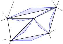
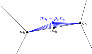
Figure 2: Sketch of the construction in Proposition 4.1. Left panel: construction of the triangles around the segments on which $\hat{z}_{j}$ jumps. Right panel: separation of one “large” jump into many smaller jumps.

The segments for which both traces are unchanged need not be treated, as well as those where both new traces are zero. The critical set is

$$H:=\{h:0=\hat{z}_{h}^{+}\neq z_{h}^{+}\text{ and }\hat{z}_{h}^{-}\neq 0\}\cup\{h:0=\hat{z}_{h}^{-}\neq z_{h}^{-}\text{ and }\hat{z}_{h}^{+}\neq 0\}.$$

As in the computation in (4.13) we obtain

$$\sum_{h\in H}|D\hat{z}_{j}|([a_{h},b_{h}])\leq M_{j}\mathcal{H}^{1}(\partial_{*}\{f_{j}>M_{j}\})\leq 2\delta.$$

For these segments we need to separate the jump into many smaller jumps. For any $h\in H$ we let $m_{h}:=(a_{h}+b_{h})/2$ be the midpoint of the segment $[a_{h},b_{h}]$, and choose $\rho_{h}\in(0,|b_{h}-a_{h}|)$ such that the triangles $T^{h}:=\mathop{\mathrm{conv}}(a_{h},b_{h},m_{h}+\rho_{h}n_{h})$ are, up to the vertices, all disjoint and their total area is less then $2^{-j}$ (see Figure 2). This is possible since there are finitely many segments.

Choose now one $h\in H$, and assume for definiteness that $\hat{z}_{h}^{-}=0$. Since $|\hat{z}_{h}^{+}|\leq M_{j}$ there are ${L_{h}}\leq M_{j}/\sigma_{j}$ and $\alpha_{l}\in\sigma_{j}(\mathbb{Z}^{N}\cap[-1,1]^{N})$, with $l=1,\dots,L_{h}$, such that $\hat{z}_{h}^{+}=\sum_{l=1}^{L_{h}}\alpha_{l}$. For $l=0,\dots,L_{h}$ we define the triangles

$$T^{h}_{l}:=\mathop{\mathrm{conv}}(a_{h},b_{h},m_{h}+{\frac{l+1}{L_{h}+1}}\rho_{h}n_{h})$$

and $v_{j}:\Omega\to\sigma_{j}\mathbb{Z}^{N}$ by setting $v_{j}=\sum_{l^{\prime}=1}^{l}\alpha_{l^{\prime}}$ on each $T^{h}_{l}\setminus T^{h}_{l-1}$, and $v_{j}=\hat{z}_{j}$ outside the union of the triangles. Then $[v_{j}]\in\sigma_{j}(\mathbb{Z}^{N}\cap[-1,1]^{N})$ on each of the closed triangles ${T^{h}}$, $v_{j}=\hat{z}_{j}$ on the outer boundary of $T^{h}$, and $|Dv_{j}|(T^{h})\leq c|a_{h}-b_{h}||\hat{z}_{h}^{+}-\hat{z}_{h}^{-}|\leq c|D\hat{z}_{j}|([a_{h},b_{h}])$. Therefore, recalling (4.14),

$$\begin{split}E^{\mathrm{LT}}_{\sigma_{j}}[v_{j},\Omega]\leq&E^{\mathrm{LT}}_{\sigma_{j}}[z_{j},\Omega]+\sum_{h\in H}\int_{\cup_{l}\partial T_{l}^{h}}\sigma_{j}\psi\left(\frac{[v_{j}]}{\sigma_{j}},\nu\right)d\mathcal{H}^{1}\\ \leq&E^{\mathrm{LT}}_{\sigma_{j}}[z_{j},\Omega]+\sum_{h\in H}\int_{\cup_{l}\partial T_{l}^{h}}\hat{c}|[v_{j}]|d\mathcal{H}^{1}\\ =&E^{\mathrm{LT}}_{\sigma_{j}}[z_{j},\Omega]+c\sum_{h\in H}|Dv_{j}|(T^{h})\\ \leq&E^{\mathrm{LT}}_{\sigma_{j}}[z_{j},\Omega]+c\sum_{h\in H}|D\hat{z}_{j}|([a_{h},b_{h}])\leq E^{\mathrm{LT}}_{\sigma_{j}}[z_{j},\Omega]+c\delta.\end{split}$$

The same computation also shows that $v_{j}$ is bounded in $BV$. Since $|\{v_{j}\neq\hat{z}_{j}\}|\leq 2^{-j}$ we obtain $v_{j}\to u$ pointwise almost everywhere. ∎

5 Upper bound

The upper bound is obtained by an explicit but involved construction, that combines the several rescaling steps. Due to the incompatibility of the two constraints of being $BV$ with values in a scaled copy of $\mathbb{Z}^{N}$ and being in $H^{1/2}$ we cannot use density and separate the two scales. Instead we need to use a joint construction, which depends on both scales.

We start from the sequence constructed in Section 4, which takes values in $SBV(\Omega;\sigma\mathbb{Z}^{N})$ for a scale $\sigma$ which converges slowly to 0 with respect to ${\varepsilon}$. The key step is the construction in the following lemma.

Lemma 5.1.

Let $\Omega\subset\subset\Omega^{\prime}$ be two bounded Lipschitz domains. Let $\sigma>0$, $v\in SBV(\Omega^{\prime};\sigma\mathbb{Z}^{N}){\cap L^{\infty}(\Omega^{\prime};\sigma\mathbb{Z}^{N})}$ polyhedral, $\alpha\in(0,{\frac{1}{2}})$ and $\rho>0$ with $3\rho^{\alpha}<{\mathrm{dist}}(\Omega,\partial\Omega^{\prime})$.

Then for any ${\varepsilon}>0$ there are $w_{\varepsilon}\in L^{2}(\Omega;\mathbb{R}^{N})$ and $\zeta\in\overline{B}_{1}$ such that

$$\|\frac{w_{\varepsilon}}{\ln(1/{\varepsilon})}\|_{L^{\infty}(\Omega)}\leq\|v\|_{L^{\infty}(\Omega)},$$

$$\|\frac{w_{\varepsilon}}{\ln(1/{\varepsilon})}-v\|_{L^{1}(\Omega)}\leq\rho^{\alpha}|Dv|(\Omega^{\prime}),$$

and

$$\limsup_{{\varepsilon}\to 0}\frac{E_{\varepsilon}[w_{\varepsilon},\Omega]}{(\ln(1/{\varepsilon}))^{2}} \leq\int_{J_{v}\cap\Omega^{\prime}}\sigma\psi\left(\frac{[v]}{\sigma},n\right)d\mathcal{H}^{1}+f(\rho)(|Dv|(\Omega^{\prime}))^{4/3}{\|v\|_{L^{\infty}(\Omega^{\prime})}^{2/3}}$$

$$+\int_{\Omega}\int_{\Omega\setminus B_{\rho}(x)} \Gamma(x-y)(v^{\zeta}_{\infty}(x)-v^{\zeta}_{\infty}(y))\cdot(v^{\zeta}_{\infty}(x)-v^{\zeta}_{\infty}(x))dydx$$

where $v^{\zeta}_{\infty}:\Omega\to\mathbb{R}^{N}$ is defined by

$$v^{\zeta}_{\infty}(x):=\int_{0}^{1}v(x+\rho^{\alpha}\zeta t)dt,$$ (5.1)

and $f(\rho)\to 0$ as $\rho\to 0$. The function $f$ depends on $\Gamma$ and $\alpha$, but not on $v$.

Proof will be given at the end of this section. The main point is to replicate each interface $\sigma\ln\frac{1}{{\varepsilon}}$ times, and then mollify on a scale ${\varepsilon}$. This modifies the function only on a small set, of area proportional to $\sigma{\varepsilon}\ln\frac{1}{{\varepsilon}}$, which ensures that the nonlinear term ${\varepsilon}^{-1}\|{\mathrm{dist}}(u_{\varepsilon},\mathbb{Z}^{N})\|_{2}^{2}$ vanishes in the limit, for an appropriate scaling of $\sigma$. Since the separation between the interfaces is much larger than the scale of the mollification, their interaction is small. For each interface, the energy is estimated by an explicit computation in Lemma 5.3.

Care must be taken in undoing the several relaxation steps, both at the line-tension and at the continuous scale, and in several truncation steps to permit to estimate the various error terms. For this construction in the upper bound we fix a mollifier $\varphi_{1}\in C^{\infty}_{c}(B_{1})$ and set $\varphi_{\lambda}:=\lambda^{-2}\varphi_{1}(\lambda x)$.

Proposition 5.2.

Let $\Omega\subset\mathbb{R}^{2}$ be a bounded connected Lipschitz domain, and let $E_{\varepsilon}[\cdot,\Omega]$ be defined as in (1.1), with $W$ and $\Gamma$ which satisfy (1.2)–(1.4).

Let $u_{0}\in BV(\Omega;\mathbb{R}^{N})\cap H^{1/2}(\Omega;\mathbb{R}^{N})$. For any ${\varepsilon}>0$ there is $u_{\varepsilon}\in L^{2}(\Omega;\mathbb{R}^{N})$ with $u_{\varepsilon}/(\ln(1/{\varepsilon}))\to u$ in $L^{2}$ and

$$\limsup_{{\varepsilon}\to 0}\frac{E_{\varepsilon}[u_{\varepsilon},\Omega]}{(\ln(1/{\varepsilon}))^{2}}\leq F_{0}[u,\Omega]\,.$$ (5.2)

We recall that $F_{0}$ was defined in (1.10).

Proof.

We start by reducing to the case that $u$ is smooth and that it is defined on a domain $\Omega^{\prime}$ larger than $\Omega$.

To see this, observe that since $\Omega$ is Lipschitz there are an open set $\omega$ with $\partial\Omega\subset\omega$ and a bilipschitz map $\Phi:\omega\to\omega$ such that $\Phi(x)=x$ for $x\in\partial\Omega$ and $\Phi(\Omega\cap\omega)=\omega\setminus\overline{\Omega}$. We define $\hat{u}:\Omega\cup\omega\to\mathbb{R}^{N}$ by reflection

$$\hat{u}:=\begin{cases}u,&\text{ in }\Omega,\\ u\circ\Phi,&\text{ in }\omega\setminus\Omega.\end{cases}$$

Then $\hat{u}\in BV(\Omega\cup\omega;\mathbb{R}^{N})\cap H^{1/2}(\Omega\cup\omega;\mathbb{R}^{N})$, with $|D\hat{u}|(\partial\Omega)=0$. We fix $\delta>0$ and let $\Omega_{\delta}:=\{x:{\mathrm{dist}}(x,\Omega)<\delta\}$, so that

$$\limsup_{\delta\to 0}|D\hat{u}|(\Omega_{\delta})=|D\hat{u}|(\Omega)=|Du|(\Omega)$$

and

$$\limsup_{\delta\to 0}\,[\hat{u}]_{H^{1/2}(\Omega_{\delta})}=[\hat{u}]_{H^{1/2}(\Omega)}=[u]_{H^{1/2}(\Omega)}.$$

In particular,

$$\limsup_{\delta\to 0}F_{0}[\hat{u},\Omega_{\delta}]=F_{0}[\hat{u},\Omega]=F_{0}[u,\Omega].$$

Now for sufficiently small $\delta$ define $u_{\delta}:=\varphi_{\delta}\ast\hat{u}\in C^{\infty}(\overline{\Omega_{\delta}};\mathbb{R}^{N})$, with $\varphi_{\delta}$ the mollification kernel. Since $F_{0}$ is convex, we have

$$\limsup_{\delta\to 0}F_{0}[u_{\delta},\Omega_{\delta}]\leq\limsup_{\delta\to 0}F_{0}[\hat{u},\Omega_{2\delta}]=F_{0}[u,\Omega]$$

and $u_{\delta}\to u$ in $L^{2}(\Omega;\mathbb{R}^{N})$.

Therefore in the rest of the proof we assume that $u\in C^{\infty}(\overline{\Omega^{\prime}};\mathbb{R}^{N})$ is given, with $\Omega\subset\subset\Omega^{\prime}$ and $\Omega^{\prime}$ Lipschitz. We shall show that for any $\eta>0$ and any ${\varepsilon}>0$ there is $w_{\varepsilon}\in L^{2}(\Omega;\mathbb{R}^{N})$ such that $w_{\varepsilon}/\ln(1/{\varepsilon})\to u$ in $L^{2}(\Omega;\mathbb{R}^{N})$ and

$$\limsup_{{\varepsilon}\to 0}\frac{1}{(\ln(1/{\varepsilon}))^{2}}E_{\varepsilon}[w_{\varepsilon},\Omega]\leq F_{0}[u,\Omega^{\prime}]+\eta.$$ (5.3)

Since $\eta$ is arbitrary, taking a diagonal subsequence will conclude the proof of (5.2).

It remains to prove (5.3). Let $\sigma_{j}\in(0,1)$ be such that $\sigma_{j}\downarrow 0$ as $j\to 0$. By Proposition 4.1 (which can be applied thanks to Lemma 4.4) there are polyhedral functions $v_{j}\in SBV(\Omega^{\prime};\sigma_{j}\mathbb{Z}^{N})$ such that $v_{j}$ converges to $u$ strongly in $L^{1}(\Omega^{\prime};\mathbb{R}^{N})$,

$$\limsup_{j\to\infty}\int_{J_{v_{j}}\cap\Omega^{\prime}}\sigma_{j}\psi\left(\frac{[v_{j}]}{\sigma_{j}},n_{j}\right)d\mathcal{H}^{1}\leq F_{\mathrm{\mathrm{self}}}[u,\Omega^{\prime}]+\eta,$$

and $C_{\eta}:=\sup\|v_{j}\|_{L^{\infty}(\Omega)}+|Dv_{j}|(\Omega^{\prime})<\infty$. We recall that, since $u$ is smooth, in particular $u\in L^{\infty}(\Omega^{\prime})$ and that $F_{\mathrm{\mathrm{self}}}[u,\Omega^{\prime}]=E^{\mathrm{LT}}_{0}[u,\Omega^{\prime}]$ (see the statements of Theorem 1.1 and Theorem 2.2).

Since $v_{j}$ is polyhedral, by Lemma 5.1 for $\alpha:=1/3$, and ${\varepsilon}$ and $\rho$ small enough, there are functions $w_{\varepsilon}^{j,\rho}\in L^{2}(\Omega;\mathbb{R}^{N})$ and vectors $\zeta_{j}\in\overline{B}_{1}$ such that

$$\|\frac{w_{\varepsilon}^{j,\rho}}{\ln(1/{\varepsilon})}\|_{L^{\infty}(\Omega)}\leq\|v_{j}\|_{L^{\infty}(\Omega)}\leq C_{\eta},$$ (5.4)

$$\|\frac{w_{\varepsilon}}{\ln(1/{\varepsilon})}-v\|_{L^{1}(\Omega)}\leq\rho^{\alpha}|Dv|(\Omega^{\prime}),$$

and

$$\limsup_{{\varepsilon}\to 0} \frac{1}{(\ln(1/{\varepsilon}))^{2}}E_{\varepsilon}[w_{\varepsilon}^{j,\rho},\Omega]$$

$$\leq \int_{J_{v_{j}}\cap\Omega^{\prime}}\sigma_{j}\psi\left(\frac{[v_{j}]}{\sigma_{j}},n_{j}\right)d\mathcal{H}^{1}+f(\rho)(|Dv_{j}|(\Omega^{\prime}))^{4/3}\|v_{j}\|_{L^{\infty}(\Omega^{\prime})}^{2/3}$$

$$+\int_{\Omega}\int_{\Omega\setminus B_{\rho}(x)}\Gamma(x-y)(v^{\zeta_{j}}_{j,\infty}(x)-v^{\zeta_{j}}_{j,\infty}(y))\cdot(v^{\zeta_{j}}_{j,\infty}(x)-v^{\zeta_{j}}_{j,\infty}(y))dydx,$$

where $v^{\zeta_{j}}_{j,\infty}=(v_{j})_{\infty}^{\zeta_{j}}$ is an average of $v_{j}$ in direction $\zeta_{j}$ at a scale set by $\rho$ as defined in (5.1). Further from (5.4)

$$\limsup_{{\varepsilon}\to 0}\|\frac{w_{\varepsilon}^{j,\rho}}{\ln(1/{\varepsilon})}-u\|_{L^{1}(\Omega)}\leq \|v_{j}-u\|_{L^{1}(\Omega)}+\limsup_{{\varepsilon}\to 0}\|\frac{w_{\varepsilon}^{j,\rho}}{\ln(1/{\varepsilon})}-v_{j}\|_{L^{1}(\Omega)}$$

$$\leq \|v_{j}-u\|_{L^{1}(\Omega)}+\rho^{\alpha}|Dv_{j}|(\Omega^{\prime})$$

$$\leq \|v_{j}-u\|_{L^{1}(\Omega)}+C_{\eta}\rho^{\alpha}.$$

We now take $j\to\infty$, and extract a subsequence such that $\zeta_{j_{k}}\to\zeta_{\infty}$ and $\displaystyle\lim_{k\to\infty}\limsup_{{\varepsilon}\to 0}\frac{1}{(\ln(1/{\varepsilon}))^{2}}E_{\varepsilon}[w_{\varepsilon}^{j_{k},\rho},\Omega]=\limsup_{j\to\infty}\limsup_{{\varepsilon}\to 0}\frac{1}{(\ln(1/{\varepsilon}))^{2}}E_{\varepsilon}[w_{\varepsilon}^{j,\rho},\Omega]$. By dominated convergence, $(v_{j})^{\zeta_{j}}_{\infty}\to u^{\zeta_{\infty}}_{\infty}$ pointwise and hence in $L^{2}(\Omega;\mathbb{R}^{N})$ and

$$\limsup_{j\to\infty}\limsup_{{\varepsilon}\to 0}\frac{1}{(\ln(1/{\varepsilon}))^{2}}E_{\varepsilon}[w_{\varepsilon}^{j,\rho},\Omega] \leq F_{\mathrm{\mathrm{self}}}[u,\Omega^{\prime}]+\eta+C_{\eta}^{2}f(\rho)$$

$$+\int_{\Omega}\int_{\Omega\setminus B_{\rho}(x)}\Gamma(x-y) (u^{\zeta_{\infty}}_{\infty}(x)-u^{\zeta_{\infty}}_{\infty}(y))\cdot(u^{\zeta_{\infty}}_{\infty}(x)-u^{\zeta_{\infty}}_{\infty}(y))dydx.$$

As $\rho\to 0$ we have, since $u\in C^{\infty}(\Omega^{\prime};\mathbb{R}^{N})$, that $u^{\zeta_{\infty}}_{\infty}\to u$ in $L^{2}(\Omega;\mathbb{R}^{N})$ and in $H^{1/2}(\Omega;\mathbb{R}^{N})$ and therefore

$$\limsup_{\rho\to 0}\limsup_{j\to\infty}\limsup_{{\varepsilon}\to 0}\frac{1}{(\ln(1/{\varepsilon}))^{2}}E_{\varepsilon}[w_{\varepsilon}^{j,\rho},\Omega] \leq F_{\mathrm{\mathrm{self}}}[u,\Omega^{\prime}]+\eta$$

$$+\int_{\Omega^{\prime}\times\Omega^{\prime}}\Gamma(x-y) (u(x)-u(y))\cdot(u(x)-u(y))dydx$$

$$=F_{0}[u,\Omega^{\prime}]+\eta$$

with

$$\limsup_{\rho\to 0}\limsup_{j\to\infty}\limsup_{{\varepsilon}\to 0}\|\frac{w_{\varepsilon}^{j,\rho}}{\ln(1/{\varepsilon})}-u\|_{L^{2}(\Omega)}=0.$$

Taking a diagonal sequence concludes the proof of (5.3). ∎

It remains to show the detailed construction of the functions $w_{\varepsilon}^{j,\rho}$ given in Lemma 5.1. First we recall that the unrelaxed line tension energy for polyhedral interfaces can be obtained with a direct computation starting from the nonlocal energy.

Lemma 5.3.

Let $\Omega\subset\subset\Omega^{\prime}$ be two bounded open sets, $v\in SBV(\Omega^{\prime};\mathbb{Z}^{N})$ polyhedral, and assume that $\Gamma$ obeys (1.3) and (1.4). Let $\varphi_{\varepsilon}\in C^{\infty}_{c}(B_{\varepsilon})$ be a mollifier and ${\varepsilon}<{\mathrm{dist}}(\Omega,\partial\Omega^{\prime})$. Then $w_{\varepsilon}:=\varphi_{\varepsilon}\ast v$ obeys

$$\limsup_{{\varepsilon}\to 0}\frac{1}{\ln(1/{\varepsilon})}\int_{\Omega\times\Omega}\Gamma(x-y)(w_{\varepsilon}(x)-w_{\varepsilon}(y))\cdot(w_{\varepsilon}(x)-w_{\varepsilon}(y))dxdy$$

$$\leq\int_{J_{v}\cap\Omega^{\prime}}\psi([v],n)d\mathcal{H}^{1},$$

where $\psi$ is as in (1.6).

Proof.

See [GM06, Section 6]. ∎

Proof of Lemma 5.1.

We choose $\Omega^{\prime\prime}$ such that $\Omega\subset\subset\Omega^{\prime\prime}\subset\subset\Omega^{\prime}$, $\rho^{\alpha}<{\mathrm{dist}}(\Omega,\partial\Omega^{\prime\prime})$, and $\rho^{\alpha}<{\mathrm{dist}}(\Omega^{\prime\prime},\partial\Omega^{\prime})$, and for $\zeta\in\overline{B}_{1}\subset\mathbb{R}^{2}$ and $L>0$ we define the functions $v^{\zeta}_{L}:\Omega^{\prime\prime}\to\frac{\sigma}{L}\mathbb{Z}^{N}$ by

$$v^{\zeta}_{L}(x):=\sum_{j=1}^{\lfloor L\rfloor}\frac{1}{L}v(x+\rho^{\alpha}\frac{j}{L}\zeta).$$

Note that $v^{\zeta}_{L}\in SBV(\Omega^{\prime\prime};\frac{\sigma}{L}\mathbb{Z}^{N})$ has jump set which is obtained by $\lfloor L\rfloor$ copies of the jump set of $v$, translated in the direction of $\zeta$, and that $\|v^{\zeta}_{L}\|_{L^{\infty}(\Omega^{\prime\prime})}\leq\|v\|_{L^{\infty}(\Omega^{\prime})}$.

We set $L_{\varepsilon}:=\sigma\ln\frac{1}{{\varepsilon}}$. For ${\varepsilon}\leq{\mathrm{dist}}(\Omega,\partial\Omega^{\prime\prime})$ we define

$$w_{\varepsilon}:={\ln(1/{\varepsilon})}v^{\zeta_{\varepsilon}}_{L_{\varepsilon}}\ast\varphi_{\varepsilon}\hskip 14.22636pt\text{ and }\hskip 14.22636pt\hat{w}_{\varepsilon}:=v^{\zeta_{\varepsilon}}_{L_{\varepsilon}}\ast\varphi_{\varepsilon}$$

(if ${\varepsilon}>{\mathrm{dist}}(\Omega,\partial\Omega^{\prime\prime})$ we can set $w_{\varepsilon}=0$), the vectors $\zeta_{\varepsilon}\in\overline{B}_{1}$ will be chosen below.

We remark that $v\in\sigma\mathbb{Z}^{N}$ almost everywhere implies $v_{L_{\varepsilon}}^{\zeta_{\varepsilon}}\in\frac{1}{L_{\varepsilon}}\sigma\mathbb{Z}^{N}=\frac{1}{\ln(1/{\varepsilon})}\mathbb{Z}^{N}$ a.e., therefore $w_{\varepsilon}(x)\in\mathbb{Z}^{N}$ for any $x$ at distance at least ${\varepsilon}$ from $J_{v^{\zeta_{\varepsilon}}_{L_{\varepsilon}}}$. Since $J_{v}$ is a finite union of segments, and ${\mathrm{dist}}(w_{\varepsilon},\mathbb{Z}^{N})\leq N^{1/2}$ everywhere, we have

$$\limsup_{{\varepsilon}\to 0}\frac{1}{{\varepsilon}(\ln(1/{\varepsilon}))^{2}}\int_{\Omega}{\mathrm{dist}}^{2}(w_{\varepsilon},\mathbb{Z}^{N})dx\leq\lim_{{\varepsilon}\to 0}\frac{\lfloor L_{\varepsilon}\rfloor\,N\,|\{x\in\Omega:{\mathrm{dist}}(x,J_{v}\cap\Omega^{\prime})<{\varepsilon}\}|}{{\varepsilon}(\ln(1/{\varepsilon}))^{2}}=0.$$

We write the long-range elastic energy as a bilinear form, $B_{LR}^{\rho}:L^{2}(\Omega;\mathbb{R}^{N})^{2}\to\mathbb{R}$,

$$B_{LR}^{\rho}(u,u^{\prime}):=\int_{\Omega}\int_{\Omega\setminus B_{\rho}(x)}\Gamma(x-y)(u(x)-u(y))\cdot(u^{\prime}(x)-u^{\prime}(y))dydx,$$

and choose a sequence ${\varepsilon}_{i}\to 0$, ${\varepsilon}_{i}>0$, such that

$$\lim_{i\to\infty}B_{LR}^{\rho}(\hat{w}_{{\varepsilon}_{i}},\hat{w}_{{\varepsilon}_{i}})=\limsup_{{\varepsilon}\to 0}B_{LR}^{\rho}(\hat{w}_{\varepsilon},\hat{w}_{\varepsilon}).$$ (5.5)

After extracting a further subsequence, we can additionally assume that $\zeta_{{\varepsilon}_{i}}\to\zeta$ for some $\zeta\in\overline{B}_{1}$. This defines the vector $\zeta$ in the statement (in terms of the vectors $\zeta_{\varepsilon}$ chosen below). We now show that

$$\hat{w}_{{\varepsilon}_{i}}\to v^{\zeta}_{\infty}\text{ strongly in $L^{2}(\Omega;\mathbb{R}^{N})$.}$$ (5.6)

To see this, we first observe that since $\|\hat{w}_{{\varepsilon}_{i}}\|_{L^{\infty}(\Omega)}\leq\|v\|_{L^{\infty}(\Omega^{\prime})}$ and $\|v_{\infty}^{\zeta}\|_{L^{\infty}(\Omega)}\leq\|v\|_{L^{\infty}(\Omega^{\prime})}$ it suffices to prove convergence in $L^{1}(\Omega;\mathbb{R}^{N})$. We write

$$\hat{w}_{{\varepsilon}_{i}}-v^{\zeta}_{\infty}=\varphi_{{\varepsilon}_{i}}\ast(v_{L_{{\varepsilon}_{i}}}^{\zeta_{{\varepsilon}_{i}}}-v_{\infty}^{\zeta_{{\varepsilon}_{i}}})+\varphi_{{\varepsilon}_{i}}\ast(v_{\infty}^{\zeta_{{\varepsilon}_{i}}}-v_{\infty}^{\zeta})+(\varphi_{{\varepsilon}_{i}}\ast v_{\infty}^{\zeta}-v_{\infty}^{\zeta})$$

and estimate the three terms separately. Convergence of the last one is immediate. Performing an explicit computation one can show that

$$\|v^{\zeta_{{\varepsilon}_{i}}}_{\infty}-v^{\zeta}_{\infty}\|_{L^{1}(\Omega^{\prime\prime})} \leq\rho^{\alpha}|Dv|(\Omega^{\prime})|\zeta_{{\varepsilon}_{i}}-\zeta|,$$

which implies $\|\varphi_{{\varepsilon}_{i}}\ast(v_{\infty}^{\zeta_{{\varepsilon}_{i}}}-v_{\infty}^{\zeta})\|_{L^{1}(\Omega)}\leq\|v_{\infty}^{\zeta_{{\varepsilon}_{i}}}-v_{\infty}^{\zeta}\|_{L^{1}(\Omega^{\prime\prime})}\to 0$. Analogously, from

$$\|v^{\zeta_{{\varepsilon}_{i}}}_{L_{{\varepsilon}_{i}}}-v^{\zeta_{{\varepsilon}_{i}}}_{\infty}\|_{L^{1}(\Omega^{\prime\prime})} \leq\frac{\rho^{\alpha}}{L_{{\varepsilon}_{i}}}|Dv|(\Omega^{\prime})+|\Omega^{\prime\prime}|\frac{L_{\varepsilon}-\lfloor L_{\varepsilon}\rfloor}{L_{\varepsilon}}\|v\|_{L^{\infty}(\Omega^{\prime\prime})}$$

and $\lim_{i_{\to}\infty}L_{{\varepsilon}_{i}}=\infty$ we obtain $\|\varphi_{{\varepsilon}_{i}}\ast(v_{L_{{\varepsilon}_{i}}}^{\zeta_{{\varepsilon}_{i}}}-v_{\infty}^{\zeta_{{\varepsilon}_{i}}})\|_{L^{1}(\Omega)}\to 0$. This concludes the proof of (5.6).

By continuity of $B_{LR}^{\rho}$, (5.5) and (5.6) imply

$$\limsup_{{\varepsilon}\to 0}B_{LR}^{\rho}(\hat{w}_{\varepsilon},\hat{w}_{\varepsilon})=\lim_{i\to\infty}B_{LR}^{\rho}(\hat{w}_{{\varepsilon}_{i}},\hat{w}_{{\varepsilon}_{i}})=B_{LR}^{\rho}(v^{\zeta}_{\infty},v^{\zeta}_{\infty}).$$

The short-range elastic energy can be correspondingly written, for a Borel set $E\subseteq\mathbb{R}^{2}$, as the bilinear form $B_{SR}^{\rho}(\cdot,\cdot,E):L^{2}(E;\mathbb{R}^{N})^{2}\to\mathbb{R}$,

$$B_{SR}^{\rho}(u,u^{\prime},E):=\int_{E}\int_{E\cap B_{\rho}(x)}\Gamma(x-y)(u(x)-u(y))\cdot(u^{\prime}(x)-u^{\prime}(y))dydx.$$

This term will lead us to the choice of $\zeta_{\varepsilon}$. We are interested in showing that for any ${\varepsilon}$ there is a choice of $\zeta\in\overline{B_{1}}$ which permits to control the quantity

$$B_{SR}^{\rho}(\hat{w}_{\varepsilon},\hat{w}_{\varepsilon},\Omega)=\frac{1}{L_{\varepsilon}^{2}}\sum_{j,j^{\prime}=1}^{\lfloor L_{\varepsilon}\rfloor}B_{SR}^{\rho}(T_{j}^{\zeta}v\ast\varphi_{\varepsilon},T_{j^{\prime}}^{\zeta}v\ast\varphi_{\varepsilon},\Omega)$$

where $T_{j}^{\zeta}$ is the translation operator, $(T_{j}^{\zeta}f)(x):=f(x+j\zeta\rho^{\alpha}/L_{\varepsilon})$. The separation introduced by the translations is on a length scale much larger than ${\varepsilon}$, but still infinitesimal (the choice of $\zeta_{\varepsilon}$ below shall implicitly ensure that it is not too small), therefore it is appropriate to treat the diagonal ($j=j^{\prime}$) terms separately. Using translation invariance we can see that the diagonal contribution is

$$B_{SR}^{\mathrm{diag}}(\zeta) :=\frac{1}{L_{\varepsilon}^{2}}\sum_{j=1}^{\lfloor L_{\varepsilon}\rfloor}B_{SR}^{\rho}(T_{j}^{\zeta}v\ast\varphi_{\varepsilon},T_{j}^{\zeta}v\ast\varphi_{\varepsilon},\Omega)$$

$$\leq\frac{\lfloor L_{\varepsilon}\rfloor}{L_{\varepsilon}^{2}}B_{SR}^{\rho}(v\ast\varphi_{\varepsilon},v\ast\varphi_{\varepsilon},\Omega^{\prime\prime})$$

$$=\frac{\lfloor L_{\varepsilon}\rfloor\sigma}{L_{\varepsilon}\ln(1/{\varepsilon})}B_{SR}^{\rho}(\sigma^{-1}v\ast\varphi_{\varepsilon},\sigma^{-1}v\ast\varphi_{\varepsilon},\Omega^{\prime\prime})$$

and in particular that the latter expression does not depend on the choice of $\zeta$. Since $\sigma^{-1}v\in SBV({\Omega^{\prime}};\mathbb{Z}^{N})$ is polyhedral and $\Gamma\geq 0$ pointwise, recalling Lemma 5.3, we obtain

$$\limsup_{{\varepsilon}\to 0}B_{SR}^{\mathrm{diag}}(\zeta)\leq\int_{J_{v}\cap\Omega^{\prime}}\sigma\psi\left(\frac{[v]}{\sigma},n\right)d\mathcal{H}^{1}$$

for any $\zeta\in\overline{B_{1}}$.

The off-diagonal contributions reduce to

$$B_{SR}^{\mathrm{cross}}(\zeta):= \frac{1}{L_{\varepsilon}^{2}}\sum_{j\neq j^{\prime}}B_{SR}^{\rho}(T^{\zeta}_{j}v\ast\varphi_{\varepsilon},T^{\zeta}_{j^{\prime}}v\ast\varphi_{\varepsilon},\Omega)$$

$$\leq \frac{1}{L_{\varepsilon}^{2}}\sum_{j\neq j^{\prime}}B_{SR}^{\rho}(v\ast\varphi_{\varepsilon},T^{\zeta}_{j-j^{\prime}}v\ast\varphi_{\varepsilon},\Omega^{\prime\prime}).$$

We average over all possible choices of the shifts $\zeta$. Precisely, we compute, using linearity of $B_{SR}^{\rho}$ in the second argument,

$$A_{\varepsilon}:= \int_{B_{1}}B_{SR}^{\mathrm{cross}}(\zeta)\varphi_{1}(\zeta)d\zeta\leq\int_{B_{1}}\frac{1}{L_{\varepsilon}^{2}}\sum_{j\neq j^{\prime}}B_{SR}^{\rho}(v\ast\varphi_{\varepsilon},\varphi_{1}(\zeta)T_{j-j^{\prime}}^{\zeta}v\ast\varphi_{\varepsilon},\Omega^{\prime\prime})d\zeta$$

$$= B_{SR}^{\rho}(v\ast\varphi_{\varepsilon},V\ast\varphi_{\varepsilon},\Omega^{\prime\prime}),$$

with

$$V(x):=\int_{B_{1}}\frac{1}{L_{\varepsilon}^{2}}\sum_{j\neq j^{\prime}}\varphi_{1}(\zeta)v(x+\frac{j-j^{\prime}}{L_{\varepsilon}}\rho^{\alpha}\zeta)d\zeta.$$

By a change of variables we obtain $V=\Phi\ast v$, where

$$\Phi(x):=\frac{1}{L_{\varepsilon}^{2}}\sum_{j\neq j^{\prime}}\frac{L_{\varepsilon}^{2}}{(j-j^{\prime})^{2}}\varphi_{\rho^{\alpha}}\left(\frac{L_{\varepsilon}}{j-j^{\prime}}x\right),$$

and then

$$A_{\varepsilon}\leq B_{SR}^{\rho}(v\ast\varphi_{\varepsilon},\Phi\ast v\ast\varphi_{\varepsilon},\Omega^{\prime\prime}).$$

We fix $p\in(2,\infty)$ and denote by $q:=p/(p-1)$ the dual exponent. Then

$$A_{\varepsilon}\leq \int_{B_{\rho}}\frac{c}{|z|^{3}}\int_{\Omega^{\prime\prime}}|(\varphi_{\varepsilon}\ast v)(x)-(\varphi_{\varepsilon}\ast v)(x+z)|$$

$$\hskip 28.45274pt\,\times|(\varphi_{\varepsilon}\ast\Phi\ast v)(x)-(\varphi_{\varepsilon}\ast\Phi\ast v)(x+z)|dxdz$$

$$\leq\int_{B_{\rho}}\frac{c}{|z|^{2-1/p}}\frac{\|v(\cdot)-v(\cdot+z)\|_{L^{p}(\Omega^{\prime\prime}_{\varepsilon})}}{|z|^{1/p}}\frac{\|(\Phi\ast v)(\cdot)-(\Phi\ast v)(\cdot+z)\|_{L^{q}(\Omega^{\prime\prime}_{\varepsilon})}}{|z|}dz,$$

with $\Omega^{\prime\prime}_{\varepsilon}:=\{x:{\mathrm{dist}}(x,\Omega^{\prime\prime})<{\varepsilon}\}$. We estimate, for small $z$,

$$\frac{\|v(\cdot)-v(\cdot+z)\|_{L^{p}(\Omega^{\prime\prime}_{\varepsilon})}^{p}}{|z|}\leq 2^{p-1}\|v\|_{L^{\infty}(\Omega^{\prime})}^{p-1}\int_{\Omega^{\prime\prime}_{\varepsilon}}\frac{|v(x)-v(x+z)|}{|z|}dx$$

$$\leq 2^{p-1}\|v\|_{L^{\infty}(\Omega^{\prime})}^{p-1}|Dv|(\Omega^{\prime})$$

and

$$\frac{\|(\Phi\ast v)(\cdot)-(\Phi\ast v)(\cdot+z)\|_{L^{q}(\Omega^{\prime\prime}_{\varepsilon})}}{|z|}\leq\|\Phi\|_{L^{q}(\mathbb{R}^{2})}|Dv|(\Omega^{\prime}),$$

so that, with $\int_{B_{\rho}}\frac{1}{|z|^{2-1/p}}dz\leq c\rho^{1/p}$, we conclude

$$A_{\varepsilon}\leq c\rho^{1/p}\|v\|_{L^{\infty}(\Omega^{\prime})}^{1/q}(|Dv|(\Omega^{\prime}))^{1+1/p}\|\Phi\|_{L^{q}(\mathbb{R}^{2})}.$$

Finally, recalling that $p>2$,

$$\|\Phi\|_{L^{q}(\mathbb{R}^{2})}\leq 2L_{\varepsilon}\sum_{j=1}^{\lfloor L_{\varepsilon}\rfloor}\frac{1}{j^{2}}\|\varphi_{\rho^{\alpha}}(\frac{L_{\varepsilon}}{j}x)\|_{L^{q}(\mathbb{R}^{2})}$$

$$\leq cL_{\varepsilon}\sum_{j=1}^{\lfloor L_{\varepsilon}\rfloor}\frac{1}{j^{2}}\left(\frac{j}{L_{\varepsilon}}\right)^{2/q}\rho^{-2\alpha\frac{q-1}{q}}$$

$$\leq cL_{\varepsilon}^{1-2/q}\sum_{j=1}^{\lfloor L_{\varepsilon}\rfloor}\frac{1}{j^{2/p}}\rho^{-2\alpha/p}$$

$$\leq cL_{\varepsilon}^{1-2/q}{L_{\varepsilon}^{1-2/p}}\rho^{-2\alpha/p}=c\rho^{-2\alpha/p}\,.$$

Therefore $A_{\varepsilon}\leq c\rho^{(1-2\alpha)/p}\|v\|_{L^{\infty}(\Omega^{\prime})}^{1/q}(|Dv|(\Omega^{\prime}))^{1+1/p}$. We finally choose $p=3$, and $\zeta_{\varepsilon}$ so that it is as good as on average, in the sense that $B_{SR}^{\mathrm{cross}}(\zeta_{\varepsilon})\leq A_{\varepsilon}$, and conclude the proof. ∎

6 Lower bound

In this Section we prove the lower bound. The idea is that the limit is given by two terms, that arise from short-range and long-range contributions to the nonlocal interaction, respectively. Indeed, one key idea in the proof of Proposition 6.1 is to localize the limiting energy and view it as a measure on $\Omega\times\Omega\subset\mathbb{R}^{4}$. One then shows that this measure can be written as the sum of two mutually singular terms, one supported on the diagonal and one supported outside the diagonal (see Figure 3). The lower bound arises from estimating separately these two terms. In the estimate of the diagonal term, which is local in the limit, we build upon techniques obtained for a different scaling in [CGM11], see Proposition 6.2 below. One important step is to iteratively mollify the functions along the sequence and to show that on most scales the mollification does not reduce significantly the $BV$ norm, which implies that the functions are approximately one-dimensional at that scale. The proof is done by showing that one can choose a scale that contains, up to higher-order terms, as much energy as the average scale, and that at the same time has a small loss of $BV$ norm, see (6.17) and (6.18) below.

Proposition 6.1.

Under the assumptions of Theorem 1.1, for any $u\in BV(\Omega;\mathbb{R}^{N})$ and any sequences ${\varepsilon}_{i}\to 0$ and $u_{i}\in L^{2}(\Omega;\mathbb{R}^{N})$ with $u_{i}/(\ln(1/{\varepsilon}_{i}))\to u$ in $L^{2}(\Omega;\mathbb{R}^{N})$ one has

$$F_{0}[u,\Omega]\leq\liminf_{i\to\infty}\frac{E_{{\varepsilon}_{i}}[u_{i},\Omega]}{(\ln(1/{\varepsilon}_{i}))^{2}}\,,$$ (6.1)

where $F_{0}$ was defined in (1.10).

The proof is based on the following local lower bound, which relates the short-range part of the energy to $F_{\mathrm{\mathrm{self}}}$.

Proposition 6.2.

Under the assumptions of Theorem 1.1, for any $u\in BV(\Omega;\mathbb{R}^{N})$ and any sequences ${\varepsilon}_{i}\to 0$ and $u_{i}\in L^{2}(\Omega;\mathbb{R}^{N})$ with $u_{i}/(\ln(1/{\varepsilon}_{i}))\to u$ in $L^{2}(\Omega;\mathbb{R}^{N})$, and any open set $\omega\subset\Omega$, one has

$$F_{\mathrm{\mathrm{self}}}[u,\omega]\leq\liminf_{i\to\infty}\frac{E_{{\varepsilon}_{i}}[u_{i},\omega]}{(\ln(1/{\varepsilon}_{i}))^{2}}\,,$$

where $F_{\mathrm{\mathrm{self}}}$ was defined in (1.11).

We postpone the proof of Proposition 6.2, and first show that it implies Proposition 6.1.

Proof of Proposition 6.1.

We can assume that the $\liminf$ in (6.1) is finite and, after passing to a subsequence, that it is a limit. By Proposition 3.1 we can assume $u\in BV(\Omega;\mathbb{R}^{N})\cap H^{1/2}(\Omega;\mathbb{R}^{N})$.

We start by localizing the energy. We denote by $\Delta:=\{(x,x):x\in\mathbb{R}^{2}\}\subset\mathbb{R}^{4}$ the diagonal set in $\mathbb{R}^{4}$ and by $P:\mathbb{R}^{4}\to\mathbb{R}^{2}$, $P(x_{1},x_{2},y_{1},y_{2}):=(x_{1},x_{2})$, the projection on the first two components. For any Borel set $E\subseteq\Omega\times\Omega$ we define

$$\mu_{i}(E):= \frac{1}{{\varepsilon}_{i}(\ln(1/{\varepsilon}_{i}))^{2}}\int_{P(E\cap\Delta)}{\mathrm{dist}}^{2}(u_{i}(x),\mathbb{Z}^{N})d\mathcal{L}^{2}(x)$$

$$+\int_{E}\Gamma(x-y)\frac{u_{i}(x)-u_{i}(y)}{\ln(1/{\varepsilon}_{i})}\cdot\frac{u_{i}(x)-u_{i}(y)}{\ln(1/{\varepsilon}_{i})}d\mathcal{L}^{4}(x,y),$$

so that $(\ln(1/{\varepsilon}_{i}))^{-2}E_{{\varepsilon}_{i}}[u_{i},\Omega]=\mu_{i}(\Omega\times\Omega)$. We observe that $\mu_{i}$ is a Radon measure, and after extracting a further subsequence we can assume that $\mu_{i}$ converges weakly in measures to some measure $\mu$, which implies $\mu(A\times A)\leq\lim_{i\to\infty}\mu_{i}(A\times A)$ for any open set $A\subseteq\Omega$. To conclude it suffices to prove that

$$F_{0}[u,\Omega]\leq\mu(\Omega\times\Omega).$$ (6.2)

In order to treat the long-range part of the interaction we define a measure $\mu_{LR}$ on $\Omega\times\Omega$ by

$$\mu_{LR}(E):=\int_{E}\Gamma(x-y)(u(x)-u(y))\cdot(u(x)-u(y))d\mathcal{L}^{4}(x,y),$$

for any Borel set $E\subseteq\Omega\times\Omega$. Since $u\in H^{1/2}(\Omega;\mathbb{R}^{N})$, we have $\mu_{LR}(\Omega{\times\Omega})<\infty$. Since $\Gamma(x-y)\xi\cdot\xi\geq 0$ for any $\xi\in\mathbb{R}^{N}$ and $(x,y)\in\Omega\times\Omega$, and (possibly extracting a further subsequence) $(u_{i}(x)-u_{i}(y))/\ln(1/{\varepsilon}_{i})$ converges pointwise to $u(x)-u(y)$ for $\mathcal{L}^{4}$-almost every $(x,y)$, by Fatou’s Lemma we obtain

$$\mu_{LR}(E)\leq\liminf_{i\to\infty}\mu_{i}(E)$$

for any Borel set $E\subseteq\Omega\times\Omega$ and in particular $\mu_{LR}(B_{r}^{(4)}(x))\leq\mu(B_{R}^{(4)}(x))$ if $r<R$ and $B_{R}^{(4)}(x)\subset\Omega\times\Omega$, where $B_{r}^{(4)}(x)$ is the four-dimensional ball of radius $r$ centered at $x\in\mathbb{R}^{4}$. Since $\mu_{LR}$ is absolutely continuous with respect to $\mathcal{L}^{4}$, we conclude

$$\mu_{LR}(E)\leq\mu(E)\text{ for any Borel set $E\subseteq\Omega\times\Omega$}.$$ (6.3)

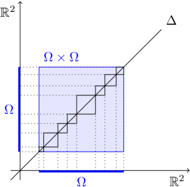
Figure 3: Sketch of the set $(\Omega\times\Omega)\cap\Delta$. The set $\Omega$ is covered (up to a null set) by finitely many balls $B_{j}$, the set $(\Omega\times\Omega)\cap\Delta$ is correspondingly covered (up to a null set) by the products $B_{j}\times B_{j}$.

We now deal with the short-range part of the energy, which concentrates on the diagonal set. We define the measure

$$\lambda:=g\left(\frac{dDu}{d|Du|}\right)|Du|$$

so that $F_{\mathrm{\mathrm{self}}}[u,E]=\lambda(E)$ for any Borel set $E\subseteq\Omega$ (we recall that $F_{\mathrm{\mathrm{self}}}$ has been defined in (1.11)). Since $u\in BV(\Omega;\mathbb{R}^{N})$, $\lambda(\Omega)<\infty$. Let $\eta>0$. For each $x\in\Omega$ there are arbitrarily small $r>0$ such that $B_{2r}(x)\subset\Omega$, $2r<\eta$, $\mu(\partial(B_{r}(x)\times B_{r}(x)))=0$ and $\lambda(\partial B_{r}(x))=0$. By Vitali’s covering theorem we can find countably many such balls, denoted by $(B_{j})_{j\in\mathbb{N}}$, such that they are pairwise disjoint, have centers in $\Delta\cap(\Omega\times\Omega)$, and

$$(\Omega\times\Omega)\cap\Delta\subseteq N\cup\bigcup_{j}(B_{j}\times B_{j})\text{ with }\mu(N)=\lambda(PN)=0$$

(see Figure 3). By Proposition 6.2 below applied with $\omega=B_{j}$ and using that $\mu(\partial(B_{j}\times B_{j}))=0$ we have

$$\lambda(B_{j})\leq\mu(B_{j}\times B_{j}).$$ (6.4)

Then, denoting $\Delta_{\eta}:=\{(x,y)\in\mathbb{R}^{2}\times\mathbb{R}^{2}:|x-y|<2\eta\}$,

$$\lambda(\Omega)=\sum_{j\in\mathbb{N}}\lambda(B_{j})\leq\sum_{j\in\mathbb{N}}\mu(B_{j}\times B_{j})\leq\mu((\Omega\times\Omega)\cap\Delta_{\eta}).$$

Since this holds for any $\eta>0$, and $\mu(\Omega\times\Omega)<\infty$, we conclude

$$\lambda(\Omega)\leq\mu((\Omega\times\Omega)\cap\Delta).$$

Recalling (6.3) and that $\mu^{LR}\ll\mathcal{L}^{4}$, we obtain $\mu_{LR}((\Omega\times\Omega)\cap\Delta)=0$ and

$$F_{0}[u,\Omega]= \lambda(\Omega)+\mu_{LR}(\Omega\times\Omega)=\lambda(\Omega)+\mu_{LR}((\Omega\times\Omega)\setminus\Delta)$$

$$\leq \mu((\Omega\times\Omega)\cap\Delta)+\mu((\Omega\times\Omega)\setminus\Delta)=\mu(\Omega\times\Omega).$$

This concludes the proof of (6.2) and therefore of the proposition. ∎

It remains to prove the local lower bound stated in Proposition 6.2. The proof uses a result from [CGM11] in which it is shown that the nonlocal energy of almost-one-dimensional $BV$ phase fields controls the line-tension energy of a similar field, that we recall in Proposition 6.3. We start by fixing a mollifier $\varphi_{0}\in C^{\infty}_{c}(B_{1};[0,\infty))$ with $\int_{B_{1}}\varphi_{0}dx=1$ and $\varphi\geq 1$ on $B_{1/2}$, and scaling it to $\varphi_{h}(x):=2^{2h}\varphi_{0}(2^{h}x)$. We remark that the index $h$ in $\varphi_{h}$ denotes the exponent, at variance with the usage in the previous part of this paper, and recall the definition of the truncated energy in (3.6).

Proposition 6.3 ([CGM11, Prop. 7.1]).

Let $\omega\subset\subset\Omega$ be two bounded open sets, $u\in W^{1,1}(\Omega;\mathbb{R}^{N})$, $M>1$, $h,t\in\mathbb{N}$ with $t\geq 3$, $\zeta\in(0,1)$. Assume ${\mathrm{dist}}(\omega,\partial\Omega)\geq 2^{-h+1}$.

Then there is $w=w_{h,\zeta,t,M}\in BV(\omega;\mathbb{Z}^{N})$ such that

$$(\ln 2)\int_{J_{w}\cap\omega}\psi_{\mathrm{rel}}([w],\nu)\,d\mathcal{H}^{1}\leq (1+\zeta+c2^{-t})E^{*}_{h+t}[u,\Omega]+\frac{C_{M}}{\zeta}2^{h+t}\|{\mathrm{dist}}(u,\mathbb{Z}^{N})\|_{L^{1}(\Omega)}$$

$$+\frac{C_{M}}{\zeta}2^{t}A^{5/6}\left(|Du|(\Omega)-|D(u\ast\varphi_{h})|(\omega)\right)^{1/6}$$

$$+\frac{c}{M^{1/2}}2^{t/2}A$$ (6.5)

and

$$\|u-w\|_{L^{1}(\omega)}\leq \frac{c}{M^{1/2}}2^{-h+t/2}A+C_{M}\|{\mathrm{dist}}(u,\mathbb{Z}^{N})\|_{L^{1}(\Omega)}$$

$$+C_{M}2^{-h}A^{2/3}\left(|Du|(\Omega)-|D(u\ast\varphi_{h})|(\omega)\right)^{1/3}\,.$$ (6.6)

Here $A:=\max\{|Du|(\Omega),E^{*}_{h+t}[u,\Omega]\}$. The constant $c$ may depend on $N$ and $\Gamma$, the constant $C_{M}$ also on $M$.

We remark that the statement of Proposition 7.1 in [CGM11] contains the unnecessary assumption that both sets are Lipschitz. The proof is based on covering $\omega$ with squares contained in $\Omega$ and performing a separate estimate on each square, in particular it never uses this assuption.

We finally give a proof of the lower bound in Proposition 6.2. The following argument is a modification of [CGM11, Prop. 8.1]. It is here used only in the case that $\omega$ is a ball.

Proof of Proposition 6.2.

It suffices to prove the estimate in the case $\omega=\Omega$ (otherwise we restrict all functions to $\omega$, and then relabel $\omega$ as $\Omega$). We can also assume that the right-hand side is finite, and extract a subsequence such that the $\liminf$ is a limit. We fix $\hat{\omega}\subset\subset\Omega$ and prove that

$$F_{\mathrm{\mathrm{self}}}[u,\hat{\omega}]\leq\liminf_{i\to\infty}\frac{E_{{\varepsilon}_{i}}[u_{i},\Omega]}{(\ln(1/{\varepsilon}_{i}))^{2}}\,.$$ (6.7)

Taking the supremum over all such sets $\hat{\omega}$ will conclude the proof.

It remains to prove (6.7). To do this we choose a Lipschitz set $\Omega^{\prime}$ such that $\hat{\omega}\subset\subset\Omega^{\prime}\subset\subset\Omega$ and fix $\delta>0$. By Proposition 3.3 for $i$ sufficiently large there are $k_{i}\in\mathbb{N}$ with

$$\varepsilon_{i}^{1-\delta/2}\leq 2^{-k_{i}}\leq\varepsilon_{i}^{1-\delta},$$ (6.8)

which implies $(1-\delta)\ln\frac{1}{{\varepsilon}_{i}}\leq k_{i}\ln 2$, and a function $v_{k_{i},\delta}\in BV(\Omega^{\prime};\mathbb{Z}^{N})$ such that

$$\lim_{i\to\infty}\|v_{k_{i},\delta}-u_{i}\|_{L^{1}(\Omega^{\prime})}\leq\lim_{i\to\infty}C2^{-k_{i}/2}\left(\ln\frac{1}{{\varepsilon}_{i}}\right)^{1/2}=0$$ (6.9)

and, with (3.7),

$$\begin{split}\liminf_{i\to\infty}\frac{1}{k_{i}^{2}}\sum_{h=0}^{k_{i}}E^{*}_{h}[v_{k_{i},\delta},\Omega^{\prime}]\leq&(\ln 2)^{2}\frac{1}{(1-\delta)^{2}}\liminf_{i\to\infty}\frac{E_{\varepsilon_{i}}[u_{i},\Omega]}{(\ln(1/{\varepsilon}_{i}))^{2}}<\infty\,.\end{split}$$ (6.10)

With (3.8) we see that there is $A_{\delta}>0$ such that

$$\frac{1}{k_{i}^{2}}\sum_{h=0}^{k_{i}}E^{*}_{h}[v_{k_{i},\delta},\Omega^{\prime}]+\frac{1}{k_{i}}|Dv_{k_{i},\delta}|(\Omega^{\prime})\leq A_{\delta}\hskip 14.22636pt\text{ for all $i\in\mathbb{N}$}\,.$$ (6.11)

For simplicity of notation in the following we write $k$ for $k_{i}$, and correspondingly $\liminf_{k\to\infty}$ for $\liminf_{i\to\infty}$.

One important idea in the proof is to define an iterated mollification of the function $v_{k,\delta}$ using a family of length scales ranging from $1$ to $2^{-k}$. We use scales separated by a factor $2^{m}$, in order to apply Proposition 6.3 between each pair of consecutive scales. The key idea is that each mollification step eliminates the structure present in the function on a certain length scale, as measured by the $BV$ norm. Since we have a $BV$ bound on the original function, and a large number of mollification steps, most of them will result in a very small reduction of the $BV$ norm, which means that on many scales the function will have an essentially one-dimensional structure. To make this precise, we fix $m\geq 3$ and define for $h\in\mathbb{N}$ the sets $\Omega_{h}:=\{x\in\mathbb{R}^{2}:{B_{2^{2-h}}}(x)\subseteq\Omega^{\prime}\}$, so that

$${\mathrm{dist}}(\Omega_{h},\partial\Omega_{h+m})\geq{\mathrm{dist}}(\Omega_{h},\partial\Omega^{\prime})-{\mathrm{dist}}(\Omega_{h+m},\partial\Omega^{\prime})\geq{2^{1-h}}.$$ (6.12)

We then define for $h\in\mathbb{N}$ the function $z_{h}\in L^{1}(\Omega_{h};\mathbb{R}^{N})$ (implicitly depending also on $k$, $\delta$, and $m$) by

$$z_{h}:=\begin{cases}v_{k,\delta},&\text{ if }h\geq k\,,\\ z_{h+m}\ast\varphi_{h},&\text{ otherwise,}\end{cases}$$

where $\varphi_{h}$ is the mollifier that enters Proposition 6.3.

One key estimate, which is obtained by summing the $m$ telescoping series and using (6.11), is

$$\begin{split}\sum_{h=0}^{k}\left[|Dz_{h+m}|(\Omega_{h+m})-|Dz_{h}|(\Omega_{h})\right]&=\sum_{h=k+1}^{k+m}|Dz_{h}|(\Omega_{h})-\sum_{h=0}^{m-1}|Dz_{h}|(\Omega_{h})\\ &\leq m|Dv_{k,\delta}|(\Omega^{\prime})\leq kmA_{\delta}\,.\end{split}$$ (6.13)

By the properties of the mollification we also obtain, for $h<k$,

$$\|z_{h}-z_{h+m}\|_{L^{1}(\Omega_{h})}=\|z_{h+m}*\varphi_{h}-z_{h+m}\|_{L^{1}(\Omega_{h})} \leq 2^{-h}|Dz_{h+m}|(\Omega_{h+m})$$

$$\leq 2^{-h}|Dv_{k,\delta}|(\Omega^{\prime})\leq k2^{-h}A_{\delta}\,,$$

and therefore

$$\|z_{h}-v_{k,\delta}\|_{L^{1}(\Omega_{h})}\leq\sum_{j=0}^{\infty}\|z_{h+jm}-z_{h+(j+1)m}\|_{L^{1}(\Omega_{h})}\leq 2k2^{-h}A_{\delta}\,.$$ (6.14)

Since $v_{k,\delta}\in\mathbb{Z}^{N}$ a.e., this implies

$$\|{\mathrm{dist}}(z_{h},\mathbb{Z}^{N})\|_{L^{1}(\Omega_{h})}\leq 2k2^{-h}A_{\delta}\,.$$ (6.15)

Convexity and translation invariance of the nonlocal energy imply that mollification decreases the energy, and using (6.12) we have

$$E^{*}_{s}[u*\varphi_{h},\Omega_{h}]\leq E^{*}_{s}[u,\Omega_{h+m}]\text{ for any }s\in\mathbb{N},\,\text{ and }u\in L^{2}(\Omega_{h+m};\mathbb{R}^{N})$$

and therefore, iterating this inequality,

$$E^{*}_{s}[z_{h},\Omega_{h}]\leq E^{*}_{s}[v_{k,\delta},\Omega^{\prime}]$$

for any $s$ and $h$. In particular,

$$E^{*}_{h+t}[z_{h+m},\Omega_{h+m}]\leq E^{*}_{h+t}[v_{k,\delta},\Omega^{\prime}].$$ (6.16)

At this point we choose $\zeta\in(0,1/4)$ and $t\in\mathbb{N}$, with $m\geq t\geq 3$. Since we shall take the limit $k\to\infty$ first, we can assume that $k\geq m/\zeta$. We now choose a good value for $h\in(\zeta k,k-\zeta k)\cap\mathbb{N}$. Specifically, let

$$J:=\{h\in(\zeta k,k-\zeta k)\cap\mathbb{N}:E^{*}_{h+t}[v_{k,\delta},\Omega^{\prime}]>(1+5\zeta)\frac{1}{k}\sum_{j=0}^{k}E^{*}_{j}[v_{k,\delta},\Omega^{\prime}]\}$$

and

$$H:=\{h\in(\zeta k,k-\zeta k)\cap\mathbb{N}:|Dz_{h+m}|(\Omega_{h+m})-|Dz_{h}|(\Omega_{h})>\frac{m}{\zeta}A_{\delta}\}.$$

One easily verifies that

$$\#J\frac{1+5\zeta}{k}\leq 1$$

and, recalling (6.13),

$$\#H\frac{1}{\zeta}\leq k.$$

We assume $\zeta\leq 1/20$, which implies $1/(1+5\zeta)\leq 1-4\zeta$, and obtain, since $\zeta k\geq m\geq 3$,

$$\#J+\#H\leq\frac{k}{1+5\zeta}+k\zeta\leq(1-2\zeta)k-3.$$

Since $\#((\zeta k,k-\zeta k)\cap\mathbb{N})\geq(1-2\zeta)k-2$, this implies that we can choose $h\in(\zeta k,k-\zeta k)\cap\mathbb{N}\setminus(J\cup H)$. This value will be fixed for the rest of the argument (depending on the other parameters) and satisfies, recalling (6.16),

$$E^{*}_{h+t}[z_{h+m},\Omega_{h+m}]\leq E^{*}_{h+t}[v_{k,\delta},\Omega^{\prime}]\leq(1+5\zeta)\frac{1}{k}\sum_{j=0}^{k}E^{*}_{j}[v_{k,\delta},\Omega^{\prime}]$$ (6.17)

and

$$|Dz_{h+m}|(\Omega_{h+m})-|Dz_{h}|(\Omega_{h})\leq\frac{m}{\zeta}A_{\delta}\,.$$ (6.18)

We apply Proposition 6.3 to $z_{h+m}$, for some $M>1$ chosen below, on the sets $\Omega_{h}\subset\subset\Omega_{h+m}$ and denote the result by $w=w_{k,\delta,m,t,M}$. We obtain

$$(\ln 2)\int_{J_{w}\cap\Omega_{h}}\psi_{\mathrm{rel}}([w],\nu)\,d\mathcal{H}^{1}\leq (1+\zeta+c2^{-t})E^{*}_{h+t}[z_{h+m},\Omega_{h+m}]$$

$$+\frac{C_{M}}{\zeta}2^{h+t}\|{\mathrm{dist}}(z_{h+m},\mathbb{Z}^{N})\|_{L^{1}(\Omega_{h+m})}$$

$$+\frac{C_{M}}{\zeta}2^{t}A_{*}^{5/6}\left(|Dz_{h+m}|(\Omega_{h+m})-|Dz_{h}|(\Omega_{h})\right)^{1/6}$$

$$+\frac{c}{M^{1/2}}2^{t/2}A_{*}$$ (6.19)

and

$$\|z_{h+m}-w\|_{L^{1}(\Omega_{h})}\leq \frac{c}{M^{1/2}}2^{-h+t/2}A_{*}+C_{M}\|{\mathrm{dist}}(z_{h+m},\mathbb{Z}^{N})\|_{L^{1}(\Omega_{h+m})}$$

$$+C_{M}2^{-h}A_{*}^{2/3}\left(|Dz_{h+m}|(\Omega_{h+m})-|Dz_{h}|(\Omega_{h})\right)^{1/3}\,,$$ (6.20)

where $A_{*}:=\max\{|Dz_{h+m}|(\Omega_{h+m}),E^{*}_{h+t}[z_{h+m},\Omega_{h+m}]\}$. Recalling (6.17), $|Dz_{h+m}|(\Omega_{h+m})\leq|Dv_{k,\delta}|(\Omega^{\prime})$ and then (6.11), we obtain

$$A_{*}\leq|Dv_{k,\delta}|(\Omega^{\prime})+\frac{2}{k}\sum_{j=0}^{k}E^{*}_{j}[v_{k,\delta},\Omega^{\prime}]\leq 2kA_{\delta}.$$ (6.21)

Then (6.20) becomes, using (6.15) and (6.18),

$$\|z_{h+m}-w\|_{L^{1}(\Omega_{h})}\leq \frac{c}{M^{1/2}}2^{-h+t/2}kA_{\delta}+C_{M}k2^{-h-m}A_{\delta}$$

$$+C_{M}2^{-h}k^{2/3}A_{\delta}m^{1/3}\zeta^{-1/3}\,.$$ (6.22)

We recall that $\hat{\omega}\subset\Omega_{h}$, for sufficiently large $k$, since we chose $h\geq k\zeta$. From (6.19), (6.17), (6.15), and (6.18),

$$\begin{split}\frac{\ln 2}{k}\int_{J_{w}\cap\hat{\omega}}\psi_{\mathrm{rel}}([w],\nu)\,d\mathcal{H}^{1}\leq&(1+\zeta+c2^{-t})(1+5\zeta)\frac{1}{k^{2}}\sum_{j=0}^{k}E^{*}_{j}[v_{k,\delta},\Omega^{\prime}]\\ &+\frac{C_{M}}{\zeta}2^{h+t}2^{-h-m}A_{\delta}\\ &+\frac{C_{M}}{k\zeta}2^{t}A_{*}^{5/6}\left(m\zeta^{-1}A_{\delta}\right)^{1/6}\\ &+\frac{c}{kM^{1/2}}2^{t/2}A_{*}\end{split}$$ (6.23)

We notice that this expression does not depend any more explicitly on the choice of $h$, since $2^{h+t}2^{-h-m}=2^{t-m}$.

We set $u^{k}:=\frac{1}{k\ln 2}w$, where $w=w_{k,\delta,m,t,M}$ is the function constructed in Proposition 6.3, so that the relaxed line-tension functional $E^{\mathrm{LT,rel}}_{\sigma}$ defined in (2.5) reads as

$$E^{\mathrm{LT,rel}}_{1/(k\ln 2)}[u^{k},\hat{\omega}]=\frac{1}{k\ln 2}\int_{J_{w}\cap\hat{\omega}}\psi_{\mathrm{rel}}([w],\nu)\,d\mathcal{H}^{1}.$$

Equation (6.23), together with (6.11) and (6.21) then yields, for sufficiently large $k$,

$$E^{\mathrm{LT,rel}}_{1/(k\ln 2)}[u^{k},\hat{\omega}] \leq\frac{1}{k^{2}(\ln 2)^{2}}\sum_{j=0}^{k}E^{*}_{j}[v_{k,\delta},\Omega^{\prime}]+(c\zeta+c2^{-t})A_{\delta}+\frac{C_{M}}{\zeta}2^{t-m}A_{\delta}$$

$$+\frac{C_{M}}{\zeta}2^{t}A_{\delta}^{5/6}\left(\frac{m}{k\zeta}A_{\delta}\right)^{1/6}+\frac{c}{M^{1/2}}2^{t/2}A_{\delta}.$$ (6.24)

Correspondingly, from (6.22) a similar procedure leads to

$$\|\frac{1}{k\ln 2}z_{h+m}-u^{k}\|_{L^{1}(\hat{\omega})}\leq \frac{c}{M^{1/2}}2^{-h+t/2}A_{\delta}+C_{M}2^{-h-m}A_{\delta}$$

$$+C_{M}2^{-h}k^{-1/3}A_{\delta}m^{1/3}\zeta^{-1/3}\,.$$ (6.25)

By (6.24) and (6.11) we obtain that $\limsup_{k\to\infty}E^{\mathrm{LT,rel}}_{1/(k\ln 2)}[u^{k},\hat{\omega}]<\infty$. Recalling $E^{\mathrm{LT,rel}}_{\sigma}\leq E^{\mathrm{LT}}_{\sigma}$ and the compactness statement in Theorem 2.2, there are $d_{k}\in\mathbb{R}^{N}$ such that, after extracting a subsequence, $u^{k}-d_{k}$ converges as $k\to\infty$ to some $u^{\delta,m,t,M}$ in $L^{1}(\hat{\omega};\mathbb{R}^{N})$. Taking the limit $k\to\infty$, and recalling Theorem 2.2 and (6.10) we obtain

$$E^{\mathrm{LT}}_{0}[u^{\delta,m,t,M},\hat{\omega}]\leq \frac{1}{(1-\delta)^{2}}\liminf_{i\to\infty}\frac{E_{\varepsilon_{i}}[u_{i},\Omega]}{(\ln(1/{\varepsilon}_{i}))^{2}}+(c\zeta+c2^{-t})A_{\delta}$$

$$+\frac{C_{M}}{\zeta}2^{t-m}A_{\delta}+\frac{c}{M^{1/2}}2^{t/2}A_{\delta}.$$ (6.26)

At the same time by (6.25) we have

$$\limsup_{k\to\infty}\|\frac{1}{k\ln 2}z_{h+m}-u^{k}\|_{L^{1}(\hat{\omega})}\leq \frac{c}{M^{1/2}}2^{-h+t/2}A_{\delta}+C_{M}2^{-h-m}A_{\delta}\,.$$

By (6.14) we have

$$\|\frac{1}{k\ln 2}z_{h+m}-\frac{1}{k\ln 2}v_{k,\delta}\|_{L^{1}(\hat{\omega})}\leq C2^{-h-m}A_{\delta}\,,$$

and therefore

$$\limsup_{k\to\infty}\|u^{k}-\frac{1}{k\ln 2}v_{k,\delta}\|_{L^{1}(\hat{\omega})}\leq\frac{c}{M^{1/2}}2^{-h+t/2}A_{\delta}+C_{M}2^{-h-m}A_{\delta}\,.$$

With (6.9), and going back to the notation where the index $i$ is explicit, we obtain

$$\limsup_{i\to\infty}\|u^{k_{i}}-\frac{1}{k_{i}\ln 2}u_{i}\|_{L^{1}(\hat{\omega})}\leq\frac{c}{M^{1/2}}2^{-h+t/2}A_{\delta}+C_{M}2^{-h-m}A_{\delta}\,,$$

so that (6.8) gives

$$\begin{split}\limsup_{i\to\infty}\|u^{k_{i}}-\frac{1}{\ln(1/{\varepsilon}_{i})}u_{i}\|_{L^{1}(\hat{\omega})}\leq&\frac{c}{M^{1/2}}2^{-h+t/2}A_{\delta}\\ &+C_{M}2^{-h-m}A_{\delta}+c\delta\limsup_{i\to\infty}\|\frac{1}{\ln(1/{\varepsilon}_{i})}u_{i}\|_{L^{1}(\hat{\omega})}\,,\end{split}$$

and since $u_{i}/\ln(1/{\varepsilon}_{i})\to u$ and $u^{k_{i}}\to u^{\delta,m,t,M}$ in $L^{2}(\hat{\omega})$,

$$\|u^{\delta,m,t,M}-u\|_{L^{1}(\hat{\omega})}\leq\frac{c}{M^{1/2}}2^{-h+t/2}A_{\delta}+C_{M}2^{-h-m}A_{\delta}+c\delta\|u\|_{L^{1}(\hat{\omega})}\,.$$

The argument is then concluded recalling (6.26) and taking a suitable diagonal subsequence. Indeed, as $\delta$, $m$, $\zeta$, $M$ and $t$ were arbitrary, and since $u^{\delta,m,t,M}\to u$, by lower semicontinuity of $F_{\mathrm{\mathrm{self}}}$ taking first $m\to\infty$, then $\zeta\to 0$, then $M\to\infty$, then $t\to\infty$, and finally $\delta\to 0$, we conclude

$$F_{\mathrm{\mathrm{self}}}[u_{0},\hat{\omega}]=E^{\mathrm{LT}}_{0}[u,\hat{\omega}]\leq \liminf_{i\to\infty}\frac{E_{\varepsilon_{i}}[u_{i},\Omega]}{(\ln(1/{\varepsilon}_{i}))^{2}}.$$

This concludes the proof of (6.7) and therefore of the Proposition. ∎

References

- [AB90a] L. Ambrosio and A. Braides. Functionals defined on partitions in sets of finite perimeter. I. Integral representation and -convergence. J. Math. Pures Appl. (9), 69:285–305, 1990.
- [AB90b] L. Ambrosio and A. Braides. Functionals defined on partitions in sets of finite perimeter. II. Semicontinuity, relaxation and homogenization. J. Math. Pures Appl. (9), 69:307–333, 1990.
- [ABS94] G. Alberti, G. Bouchitté, and P. Seppecher. Un résultat de perturbations singulières avec la norme . C. R. Acad. Sci. Paris Sér. I Math., 319:333–338, 1994.
- [ABS98] G. Alberti, G. Bouchitté, and P. Seppecher. Phase transition with the line-tension effect. Arch. Rational Mech. Anal., 144:1–46, 1998.
- [ACGO18] P. Ariza, S. Conti, A. Garroni, and M. Ortiz. Variational modeling of dislocations in crystals in the line-tension limit. In V. Mehrmann and M. Skutella, editors, European Congress of Mathematics, Berlin, 2016, pages 583–598. EMS, 2018.
- [Ach10] A. Acharya. New inroads in an old subject: plasticity, from around the atomic to the macroscopic scale. J. Mech. Phys. Solids, 58:766–778, 2010.
- [ACP11] R. Alicandro, M. Cicalese, and M. Ponsiglione. Variational equivalence between Ginzburg-Landau, spin systems and screw dislocations energies. Indiana Univ. Math. J., 60:171–208, 2011.
- [AFP00] L. Ambrosio, N. Fusco, and D. Pallara. Functions of Bounded Variation and Free Discontinuity Problems. Mathematical Monographs. Oxford University Press, 2000.
- [BCG17] A. Braides, S. Conti, and A. Garroni. Density of polyhedral partitions. Calc. Var. Part. Diff. Eq., 56:28, 2017.
- [Ber16] V. Berdichevsky. Energy of dislocation networks. International Journal of Engineering Science, 103:35–44, 2016.
- [BJOS12] S. Baldo, R. L. Jerrard, G. Orlandi, and H. M. Soner. Convergence of Ginzburg-Landau functionals in three-dimensional superconductivity. Arch. Ration. Mech. Anal., 205:699–752, 2012.
- [BJOS13] S. Baldo, R. L. Jerrard, G. Orlandi, and H. M. Soner. Vortex density models for superconductivity and superfluidity. Comm. Math. Phys., 318:131–171, 2013.
- [CG09] S. Cacace and A. Garroni. A multi-phase transition model for the dislocations with interfacial microstructure. Interfaces Free Bound., 11:291–316, 2009.
- [CG15] S. Conti and P. Gladbach. A line-tension model of dislocation networks on several slip planes. Mechanics of Materials, 90:140–147, 2015.
- [CGM11] S. Conti, A. Garroni, and S. Müller. Singular kernels, multiscale decomposition of microstructure, and dislocation models. Arch. Rat. Mech. Anal., 199:779–819, 2011.
- [CGM15] S. Conti, A. Garroni, and A. Massaccesi. Modeling of dislocations and relaxation of functionals on 1-currents with discrete multiplicity. Calc. Var. PDE, 54:1847–1874, 2015.
- [CGM16] S. Conti, A. Garroni, and S. Müller. Dislocation microstructures and strain-gradient plasticity with one active slip plane. J. Mech. Phys. Solids, 93:240–251, 2016.
- [CGM17] S. Conti, A. Garroni, and S. Müller. Homogenization of vector-valued partition problems and dislocation cell structures in the plane. Boll. Unione Mat. Ital., 10:3–17, 2017.
- [CGO15] S. Conti, A. Garroni, and M. Ortiz. The line-tension approximation as the dilute limit of linear-elastic dislocations. Arch. Ration. Mech. Anal., 218:699–755, 2015.
- [Dal93] G. Dal Maso. An introduction to -convergence. Progress in Nonlinear Differential Equations and their Applications, 8. Birkhäuser Boston Inc., Boston, MA, 1993.
- [DGP12] L. De Luca, A. Garroni, and M. Ponsiglione. -convergence analysis of systems of edge dislocations: the self energy regime. Arch. Ration. Mech. Anal., 206:885–910, 2012.
- [DNPV12] E. Di Nezza, G. Palatucci, and E. Valdinoci. Hitchhiker’s guide to the fractional Sobolev spaces. Bull. Sci. Math., 136:521–573, 2012.
- [Fed69] H. Federer. Geometric measure theory. Die Grundlehren der mathematischen Wissenschaften, Band 153. Springer-Verlag New York Inc., New York, 1969.
- [FG07] M. Focardi and A. Garroni. A 1D macroscopic phase field model for dislocations and a second order -limit. Multiscale Model. Simul., 6:1098–1124, 2007.
- [FH93] N. A. Fleck and J. W. Hutchinson. A phenomenological theory for strain gradient effects in plasticity. J. Mech. Phys. Solids, 41:1825–1857, 1993.
- [GA05] M. E. Gurtin and L. Anand. A theory of strain-gradient plasticity for isotropic, plastically irrotational materials. I. Small deformations. J. Mech. Phys. Solids, 53:1624–1649, 2005.
- [GGI10] I. Groma, G. Györgyi, and P. D. Ispánovity. Variational approach in dislocation theory. Philosophical Magazine, 90:3679–3695, 2010.
- [GGK07] I. Groma, G. Györgyi, and B. Kocsis. Dynamics of coarse grained dislocation densities from an effective free energy. Philosophical Magazine, 87:1185–1199, 2007.
- [Gin19a] J. Ginster. Plasticity as the -limit of a two-dimensional dislocation energy: the critical regime without the assumption of well-separateness. Arch. Ration. Mech. Anal., 233:1253–1288, 2019.
- [Gin19b] J. Ginster. Strain-gradient plasticity as the -limit of a nonlinear dislocation energy with mixed growth. SIAM J. Math. Anal., 51:3424–3464, 2019.
- [GLP10] A. Garroni, G. Leoni, and M. Ponsiglione. Gradient theory for plasticity via homogenization of discrete dislocations. J. Eur. Math. Soc. (JEMS), 12:1231–1266, 2010.
- [GM05] A. Garroni and S. Müller. -limit of a phase-field model of dislocations. SIAM J. Math. Anal., 36:1943–1964, 2005.
- [GM06] A. Garroni and S. Müller. A variational model for dislocations in the line tension limit. Arch. Ration. Mech. Anal., 181:535–578, 2006.
- [HL68] J. P. Hirth and J. Lothe. Theory of Dislocations. McGraw-Hill, New York, 1968.
- [Hoc13] T. Hochrainer. Moving dislocations in finite plasticity: a topological approach. ZAMM Z. Angew. Math. Mech., 93:252–268, 2013.
- [KCO02] M. Koslowski, A. M. Cuitiño, and M. Ortiz. A phase-field theory of dislocation dynamics, strain hardening and hysteresis in ductile single crystal. J. Mech. Phys. Solids, 50:2597–2635, 2002.
- [KK16] B. Kirchheim and J. Kristensen. On rank one convex functions that are homogeneous of degree one. Arch. Ration. Mech. Anal., 221:527–558, 2016.
- [KO04] M. Koslowski and M. Ortiz. A multi-phase field model of planar dislocation networks. Model. Simul. Mat. Sci. Eng., 12:1087–1097, 2004.
- [LL16] G. Lauteri and S. Luckhaus. An energy estimate for dislocation configurations and the emergence of Cosserat-type structures in metal plasticity. Preprint arXiv:1608.06155, 2016.
- [MSZ14] S. Müller, L. Scardia, and C. I. Zeppieri. Geometric rigidity for incompatible fields and an application to strain-gradient plasticity. Indiana Univ. Math. J., 63:1365–1396, 2014.
- [MSZ15] S. Müller, L. Scardia, and C. I. Zeppieri. Gradient theory for geometrically nonlinear plasticity via the homogenization of dislocations. In S. Conti and K. Hackl, editors, Analysis and Computation of Microstructure in Finite Plasticity, pages 175–204. Springer, 2015.
- [MSZ16] M. Monavari, S. Sandfeld, and M. Zaiser. Continuum representation of systems of dislocation lines: A general method for deriving closed-form evolution equations. J. Mech. Phys. Solids, 95:575–601, 2016.
- [OR99] M. Ortiz and E. Repetto. Nonconvex energy minimization and dislocation structures in ductile single crystals. J. Mech. Phys. Solids, 47:397–462, 1999.
- [Ort99] M. Ortiz. Plastic yielding as a phase transition. J. Appl. Mech.-Trans. ASME, 66:289–298, 1999.
- [Pon07] M. Ponsiglione. Elastic energy stored in a crystal induced by screw dislocations: from discrete to continuous. SIAM J. Math. Anal., 39:449–469, 2007.
- [SS03] E. Sandier and S. Serfaty. Limiting vorticities for the Ginzburg-Landau equations. Duke Math. J., 117:403–446, 2003.
- [SS07] E. Sandier and S. Serfaty. Vortices in the magnetic Ginzburg-Landau model. Progress in Nonlinear Differential Equations and their Applications, 70. Birkhäuser Boston, Inc., Boston, MA, 2007.
- [SV12] O. Savin and E. Valdinoci. -convergence for nonlocal phase transitions. Ann. Inst. H. Poincaré Anal. Non Linéaire, 29:479–500, 2012.
- [SvG16] R. Scala and N. van Goethem. Currents and dislocations at the continuum scale. Methods Appl. Anal., 23:1–34, 2016.