Improving the background estimation technique in the GstLAL inspiral pipeline with the time-reversed template bank

Abstract

Background estimation is important for determining the statistical significance of a gravitational-wave event. Currently, the background model is constructed numerically from the strain data using estimation techniques that insulate the strain data from any potential signals. However, as the observation of gravitational-wave signals become frequent, the effectiveness of such insulation will decrease. Contamination occurs when signals leak into the background model. In this work, we demonstrate an improved background estimation technique for the searches of gravitational waves (GWs) from binary neutron star coalescences by time-reversing the modeled GW waveforms. We found that the new method can robustly avoid signal contamination at a signal rate of about one per 20 seconds and retain a clean background model in the presence of signals.

I Introduction

On September 14, 2015, the first detection of gravitational-wave (GW) signal from the binary black hole (BBH) coalescence et al. (The LIGO Scientific Collaboration and the Virgo Collaboration) proved that the BBH mergers occur in the nature and providing us with another way to study the properties of BHs. Two years later, on August 17, 2017, the GWs and the accompanied electromagnetic waves from a binary neutron star (BNS) coalescence et al. (LIGO Scientific Collaboration and Collaboration, LIGO Scientific Collaboration and Collaboration) were also detected for the first time, marking the start of multi-messenger astronomy informed by GWs. To date, there are more than 10 GW events due to compact binary mergers were observed in the first two observing runs Abbott et al. (2019), and over 50 public alerts of GWs were issued during the third observing run gra , including an event from a BBH with unequal masses Abbott et al. (2020a); these discoveries have confirmed the possibility of detecting GWs with advanced GW detectors such as LIGO Aasi et al. (2015), Virgo Acernese et al. (2014), and KAGRA Aso et al. (2013). The question of whether GW exist or not is no longer a concern; instead, the question becomes how do we detect more GW signals and make more confident detections.

The detection of compact object merger signals is accomplished in part by perpendicular projection of the data onto the space of waveforms comprising the family of merger signals of interest; the magnitude of the projection is referred to as the signal-to-noise ratio (SNR) Maggiore (2008). When the SNR crosses a chosen threshold, a signal candidate, often called a “trigger” is defined and subjected to further, more computationally costly, scrutiny that ultimately leads the assignment of a detection ranking statistic. Since the geometry of the family of merger waveforms is not well understood, the perpendicular projection of the data onto their space is approximated by brute-force projection of the data onto each of a large number of members drawn uniformly from the space, collectively referred to as a template bank Sathyaprakash and Dhurandhar (1991); Owen (1996); Owen and Sathyaprakash (1999); Cokelaer (2007); Prix (2007); Harry et al. (2009); Ajith et al. (2014).

To complete the detection process, we are required to estimate the probability that the noise produces a GW trigger with a ranking statistic value larger than or equal to a pre-defined threshold; this probability is known as the false-alarm probability (FAP) and it describes the statistical significance of a GW event. The computation of FAP requires the knowledge of a background model that describes the statistical properties of noise-induced GW triggers. If the detector noise is stationary and Gaussian, the FAP of an event can be computed analytically from the matched-filtering SNR. However, real detector noise is known to be non-stationary and non-Gaussian over a long period of time Abbott et al. (2016, 2020b). In this case, we cannot assume that the SNR of the noise triggers are $\chi$-distributed random variables with two degrees of freedom.

There are various techniques to numerically estimate the background model from the strain data itself Usman et al. (2016); Sachdev et al. (2019). These techniques try to avoid picking up any potential signals as noise samples when constructing the background model. If signals are included in the background model, the search pipeline will incorrectly believe that the noise process is capable of producing more false alarms, making the significance estimation more difficult Capano et al. (2017). The problem could become worse if the background model is contaminated by too many signals. This will be the case for these techniques as the rate of detectable GW signals increases, and it can be seen from the analyses described in section IV.

If there existed an alternate space that is orthogonal to the space of merger waveforms, and that projections onto the alternate space is insensitive to the presence of genuine signals, but for which the statistical properties of quantities derived from the projection, such as the SNR, remained the same as for the projection onto the true merger waveform space, then we could construct the background model from a template bank obtained from that alternate space and not worry about signal contamination.

It is our conjecture that such spaces exist, and we prove this to be true for the specific case of BNS signals by explicit construction. We show that the use of a time-reversed version of the complete BNS template bank provides an effective background model that is nearly completely insulated from the presence of signals in the data. The statistical properties of the triggers, such as the SNR ($\rho$) and the signal consistency test value ($\xi^{2}$), from the outputs of the matched filtering with time-reversed template bank can be used directly to construct the background model. We illustrate more on the method in the next section.

This paper is organized as follows. In section II, we explain qualitatively the rationale of using time-reversed template banks to model the background, and provide proof via an example. In section III, we describe our experimental setup for the analyses. In section IV, we demonstrate the robustness of the improved method in an analysis with an unrealistic signal rate, where about 30000 software simulated BNS signals were injected into a week of strain data. We also demonstrate an application of our method in another analysis with a realistic signal rate of one per 1.75 days. Throughout the paper, the data used in each analysis was real strain data from the second observing run.

II Method

II.1 Time-Reversed Template

Using the convolution theorem, the matched-filtering in time-domain is a cross-correlation of the whitened data and whitened templates, which is defined as

$$z_{i}(t)=\int_{-\infty}^{\infty}\hat{g}^{*}_{i}(\tau)\hat{d}(\tau+t)d\tau$$ (1)

where the hat denotes the whitening process using the single-sided power spectrum density $S_{n}(f)$:

$$\hat{d}(t)=\int_{-\infty}^{\infty}\frac{\tilde{d}(f)}{\sqrt{S_{n}(|f|)/2}}e^{2\pi ift}df$$ (2)

for both strain data $d(t)$ and the $i^{th}$ complex template $g_{i}(t)$; each component of $g_{i}(t)$, which corresponds to the plus and cross polarizations, is also normalized to unity in GstLAL. The modulus of Equation (1) is the SNR time series $\rho(t)$ for each template.

In addition, the ranking statistic used in the GstLAL pipeline also takes a parameter: $\xi^{2}$ that we colloquially call it “chi-squared”. It is designed to characterize how closely the SNR time series resembles the expected SNR time series computed from the template autocorrelation. It is defined as Sachdev et al. (2019)

$$\xi_{i}^{2}=\frac{\int_{-\delta t}^{\delta t}|z_{i}(t)-R_{i}(t)|^{2}dt}{\int_{-\delta t}^{\delta t}(2-2|R_{i}(t)|^{2})dt}$$ (3)

where $\delta t$ is a tunable time window and $R_{i}(t)$ is the template autocorrelation function defined by

$$R_{i}(t)=\int_{-\infty}^{\infty}\frac{|\tilde{g}_{i}(f)|^{2}}{S_{n}(|f|)}e^{2\pi ift}df.$$ (4)

The $\rho$ and $\xi^{2}$ are mostly the quantities that are used to numerically construct the background model. Hence, it is our goal to construct an estimate of the background statistic of $\rho$ and $\xi^{2}$.

We propose using the time-reversed version of original search template bank to construct the background model for BNS searches because of the following reasons. First, the inspiral-merger stage of a low mass binary such as BNS is typically of the order of hundreds of seconds, and the chirp waveform is not symmetric in time. The inner product of a original (forward) template and its time-reversed copy will be small. Matched-filtering with a time-reversed template will cause the peaks in the SNR time series produced by the signals to be strongly suppressed. Second, the features in the original waveform such as the amplitude and duration are not lost. The response of matched filter to the Gaussian noise and glitches (at least for a time-symmetric glitch as we have shown in the following example) should remain similar.

II.2 Responses to Signals

As a demonstration that the time-reversed template is not sensitive to signals, we inject simulated GW signals from BNS, generated from TaylorF2 waveform family Buonanno et al. (2009), into the strain data every 100 seconds, and perform matched-filtering with a template that has the same parameters as the injections. The strain data is a segment of real data from LIGO Livingston detector around the event GW170817 et al. (LIGO Scientific Collaboration and Collaboration), which was known to contain a glitch. The injected GW signals are spinless BNS located uniformly from 90 Mpc to 100 Mpc and have the same masses of about $1.78M_{\odot}$ and $1.08M_{\odot}$; the range of distance is chosen that the BNS can produce visually recognizable peaks, and the value of the masses is unimportant as long as they represent the mass of a typical BNS, but we chose them to be the same masses as the event GW170817. The output of the matched-filtering using the time-reversed template and the original template is shown in Figure 1.

The result shows that the injections and the real signal produce visually prominent peaks (circles in Figure 1) in the SNR time series when filtering with the original template that matches the injections and real signal, but none of those peaks are identified in the case of time-reversed template. Moreover, the glitch, which is highlighted by a pink box in Figure 1, still persists in the output of matched-filtering using time-reversed template, but occurs at a different time and it is time-reversed as well; this indicates that the glitch is time-symmetric. However, the time of occurrence of the glitch is irrelevant; we are only concerned about the matched-filitering statistic, and a time-reversed matched-filtering output for the glitch does not affect the statistic. Therefore, the result suggests that the time-reversed version of the original template is insensitive to the injections and the real signal even though the original template has parameters that match the signal, and the statistics of a time-symmetric glitch can be preserved.

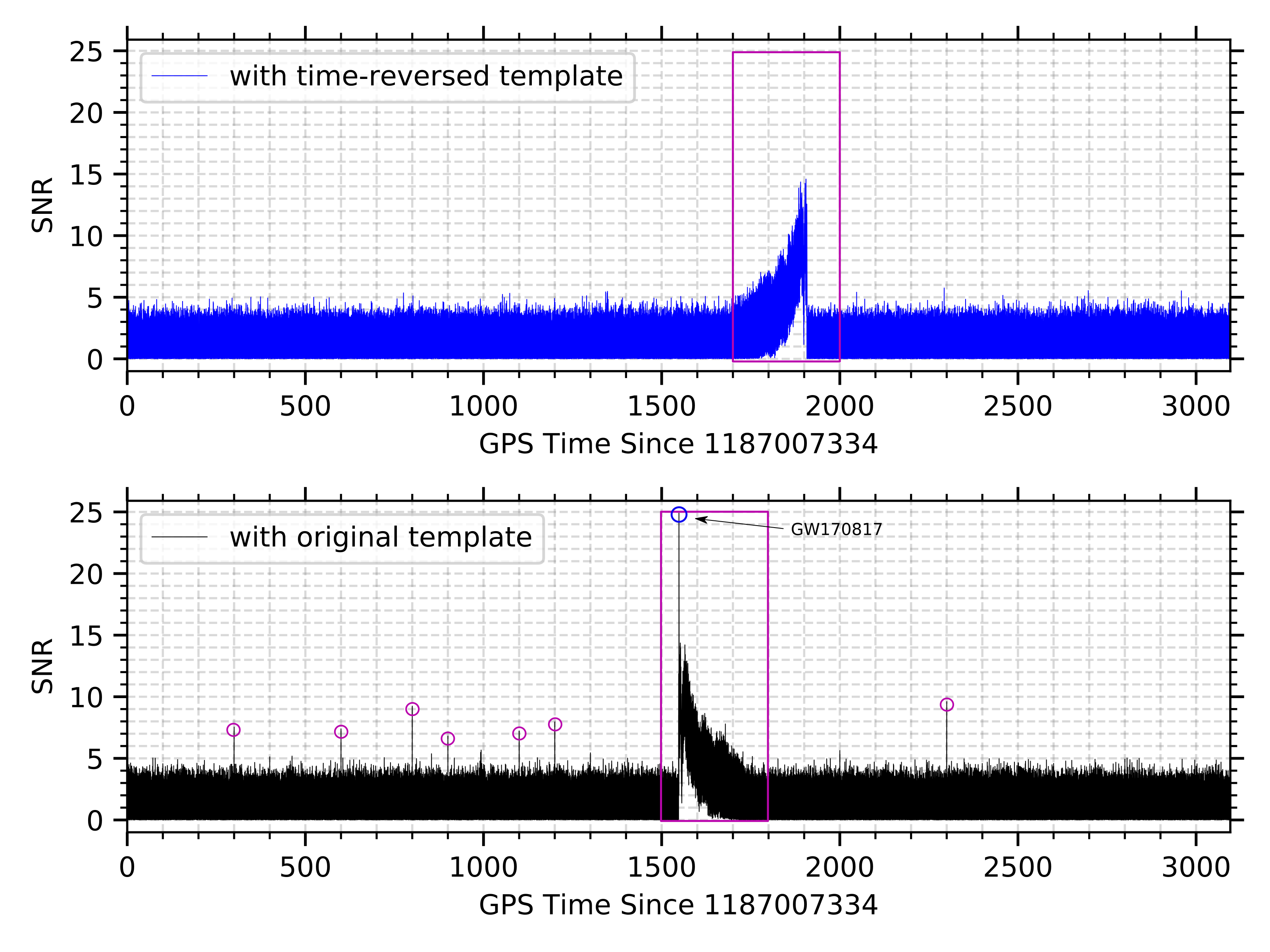
Figure 1: The matched-filter output using the time-reversed template (upper row) and the original template (bottom row). The “peaks” marked by the pink circles represent the injected signals that are identified with visually prominent SNR; the blue circle represents the event GW170817. The region marked by the pink boxes is the matched-filtering response of a time-symmetric glitch. It persists in the matched-filitering outputs of both original and time-reversed template, but occurs in different time and is time-reversed.

II.3 Responses to Noise

To show the matched-filter’s response against noise, we histogrammed the previous result and normalized it by the total counts. Figure 2 shows the statistical distribution of SNRs produced by the original and time-reversed templates. Although the data is injected with simulated signals, the SNRs contributed by the simulations are the minorities when comparing to the SNRs produced by the noise component of the data. Thus, the SNR contributed by the simulations is small compared to the SNR contributed by noise.

From the histogram, we note the distribution of SNRs of the original and time-reversed template agrees well with each other. This ensures that the time-reversed templates preserve the SNR distribution for noise, and it should not negatively impact the evaluation of likelihood ratio and FAP and/or FAR .

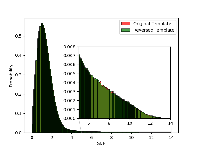
Figure 2: The histogram of SNRs with a uniform binning of size 0.1 for both original template and time-reversed template. The SNR produced by the time-reversed template agrees well with the one produced by the original template.

III Tests

III.1 Experimental Setup

The matched-filter’s responses to signals and noise for the time-reversed template have presented evidence that it is insensitive to the GW signals and able to remain the noise statistic for one template. We would like extend it to a complete GstLAL inspiral offline search and examine the performance of modeling background using a time-reversed template bank.

The background collection infrastructure was slightly modified to allow the collection of background during the times when only one detector is online (single-detector times). The modification is intended to show that the current technique should not collect background samples during single-detector times as it is impossible to form coincidences with single detector. Nevertheless, the improved technique using a time-reversed template bank should possess the ability to use the data during single-detector times even if signals are present.

III.1.1 Template Bank

Banks of search templates are generated from the TaylorF2 post-Newtonian waveform family Buonanno et al. (2009) and SEOBNRv4_ROM Bohé et al. (2017). For binaries with chirp mass $0.0M_{\odot}\leq\mathcal{M}\leq 1.73M_{\odot}$, the templates are generated with TaylorF2. For binaries with chirp mass $1.73M_{\odot}<\mathcal{M}\leq 1000.0M_{\odot}$, the templates are instead generated with SEOBNRv4_ROM. The template bank is comprised of 69781 templates covering a wide range of masses, including the BNS range. The time-reversed template bank is constructed from the same search template bank.

Mass 1 ($\text{M}_{\odot}$)	Mass 2 ($\text{M}_{\odot}$)	Spin 1	Spin 2	Detector	GPS Time	Distance (Mpc)
$1.4096$	$1.4036$	$0$	$0$	H1	1176297508	170.6
$1.4031$	$1.4078$	$0$	$0$	H1	1176457885	26.9
$1.3987$	$1.4063$	$0$	$0$	L1	1176587931	103.4
$1.3978$	$1.4127$	$0$	$0$	H1	1176739231	54.2

Table 1: The four BNS injections in the injection set B. The first fours columns are the masses and spins of the injections, and the last two columns are the times where the injections were added and the distances from Earth. The column “Detector” represents which detector was on for detection during the injection time.

III.1.2 Gravitational Wave Data

We use a week of strain data from Hanford (H1) and Livingston (L1) in the second observing run, beginning on April 14 21:25:00 GMT 2017 and ending on April 21 21:25:00 GMT 2017 et al. (LIGO Scientific Collaboration and Collaboration). This chunk of data is found to contain no significant events by the GstLAL inspiral pipeline using the search template bank mentioned in III.1.1, so a collection of software simulated GW signals from BNS will be added to the data to mimic the presence of actual GW signals; these injections are generated from the TaylorT4ThreePointFivePN waveform model. There are two injection sets prepared for the analysis, each serving a different purpose.

III.1.3 Injection Set A

Injection set A contains 30240 spinless binary sources with typical neutron star (about 1.4 $\text{M}_{\odot}$) located uniformly in distance and ranged from 20 Mpc to 200 Mpc. The masses of these injections were generated from a Gaussian distribution with a mean of 1.4 $\text{M}_{\odot}$ and a standard deviation of 0.1 $\text{M}_{\odot}$. Injections were added every 20s without considering detector duty cycles. Due to detector downtime, only 20592 injections occur at times the detectors were observing. The amount of injections over a week of data is unrealistic, but it can serve as a test for the robustness of the background estimation technique with time-reversed template bank (henceforth referred to as the improved technique).

III.1.4 Injection Set B

Injection set B contains only 4 spinless BNS sources having the parameters listed in Table 1. These injections were specifically added to the strain data during single-detectors times. The improved technique should be able to use the triggers during the single-detector times to model the background without contaminating it with signal-like triggers. Therefore, injection set B serves as a test to determine whether or not the improved technique can achieve that goal. The rate of the GW signals in this test (4 BNS injections in a week of data) is realistic when considering the mean rate of events detected by GstLAL during the third observing run. So the test can be used to demonstrate the usefulness of the improved technique in a practical situation.

III.1.5 Searches

For the following searches, we define the original technique as the background estimation technique with original templates and the improved technique as the background estimation technique with time-reversed templates.

IV Search Results and Discussion

IV.1 The Search with Severe Signal Contamination

To test the robustness of the improved technique, injection set A was added to the original data for the analysis. In this subsection, we will first show the result of the search using the original technique. Then, the result of the same search using the improved technique will be shown for comparison.

IV.1.1 Searches with Original Technique

As a reference, we first conducted the search using the original technique. The result of the search is summarized in the plot of the event counts versus $\text{ln}\mathcal{L}$ threshold (Figure 3 : top). From the figure, we note that the curve of the observed event count starts to deviate from the noise model prediction at around $\text{ln}\mathcal{L}=-4$, suggesting that there are more events observed with a $\text{ln}\mathcal{L}$ above that threshold than the prediction by the noise model. Since the observed events could be thought of as the sum of signal and noise events, the extra events will be the signal-like events. To properly define the meaning of a true GW event, we can require that all true GW events to have a FAR $\leq 3.858\times 10^{-7}$ (1 false alarm per 30 days). With this threshold, we found that 2191 events were below the threshold, meaning that only about $10.6\%$ injections were recovered by the original search pipeline.

IV.1.2 Searches with Improved Technique

Next, we performed the search again but using the improved technique. The event count versus $\text{ln}\mathcal{L}$ threshold plot (Figure 3 : bottom) shows more injections were recovered and with higher $\text{ln}\mathcal{L}$. If we set the same FAR threshold for the events to be true GW events, then there were 6990 events below the threshold, which means $33.9\%$ injections are recovered. Therefore, the improved technique is able to find more injections than the original technique.

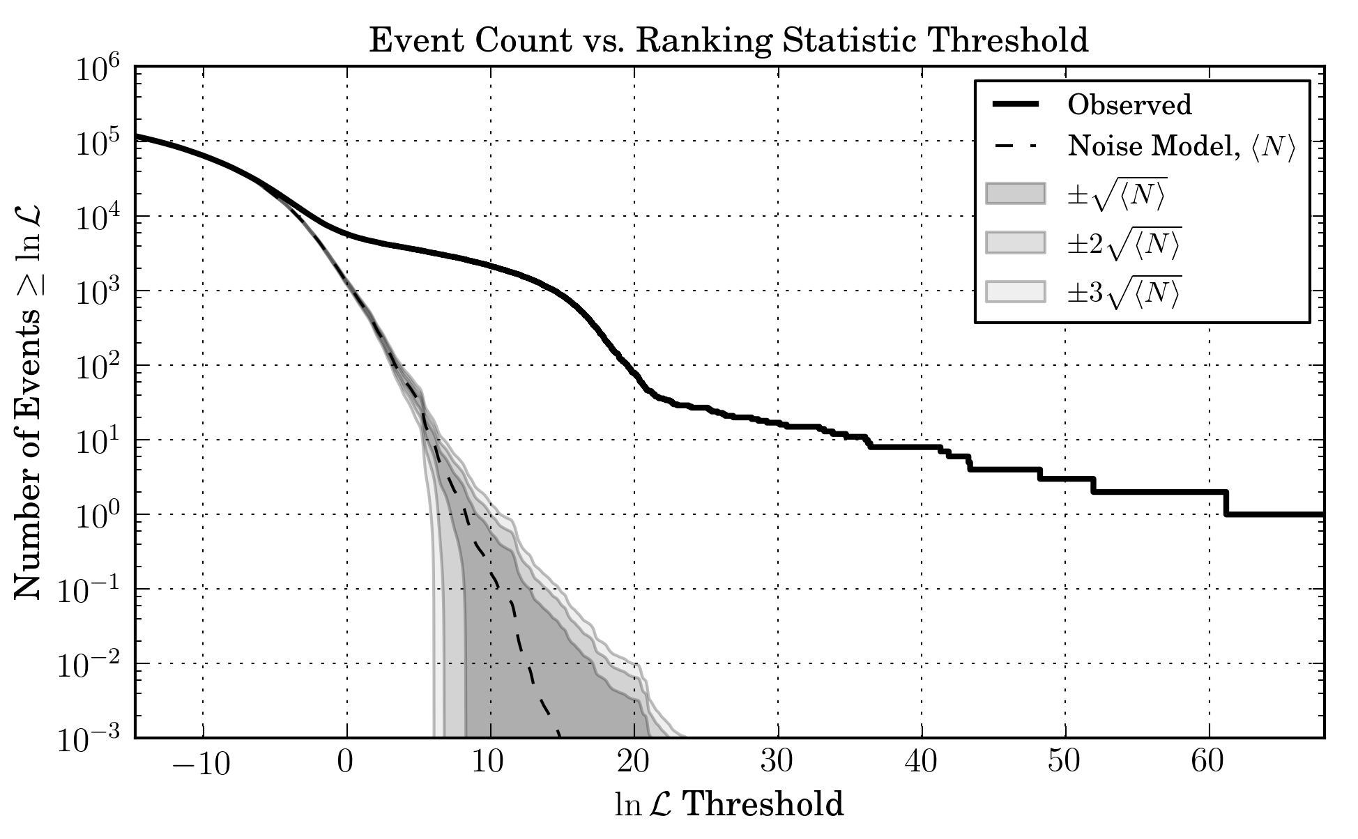
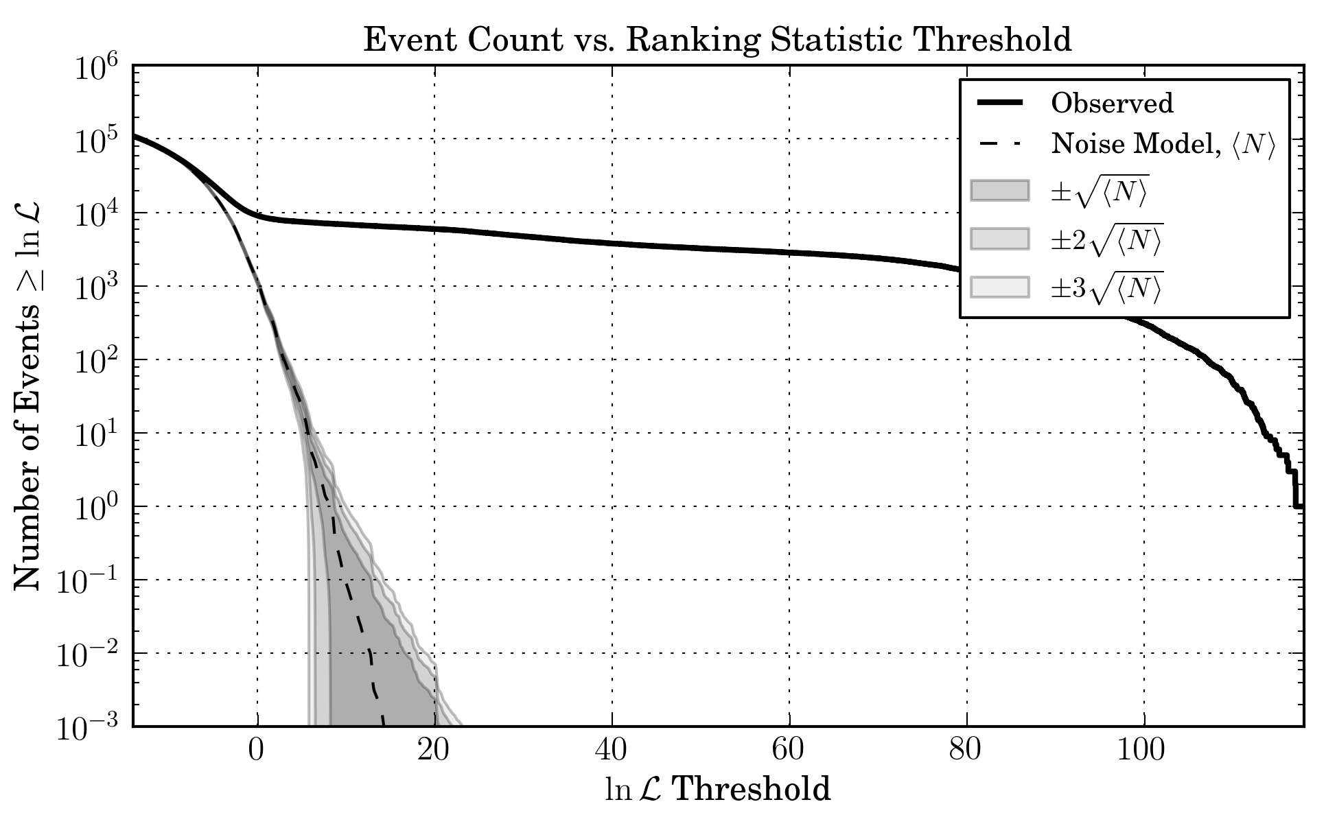
Figure 3: The plots of the event count vs. ranking statistic threshold for the injection analysis using the original technique (top) and improved technique (bottom). There are more injections identified with the improved technique compared to the original technique.

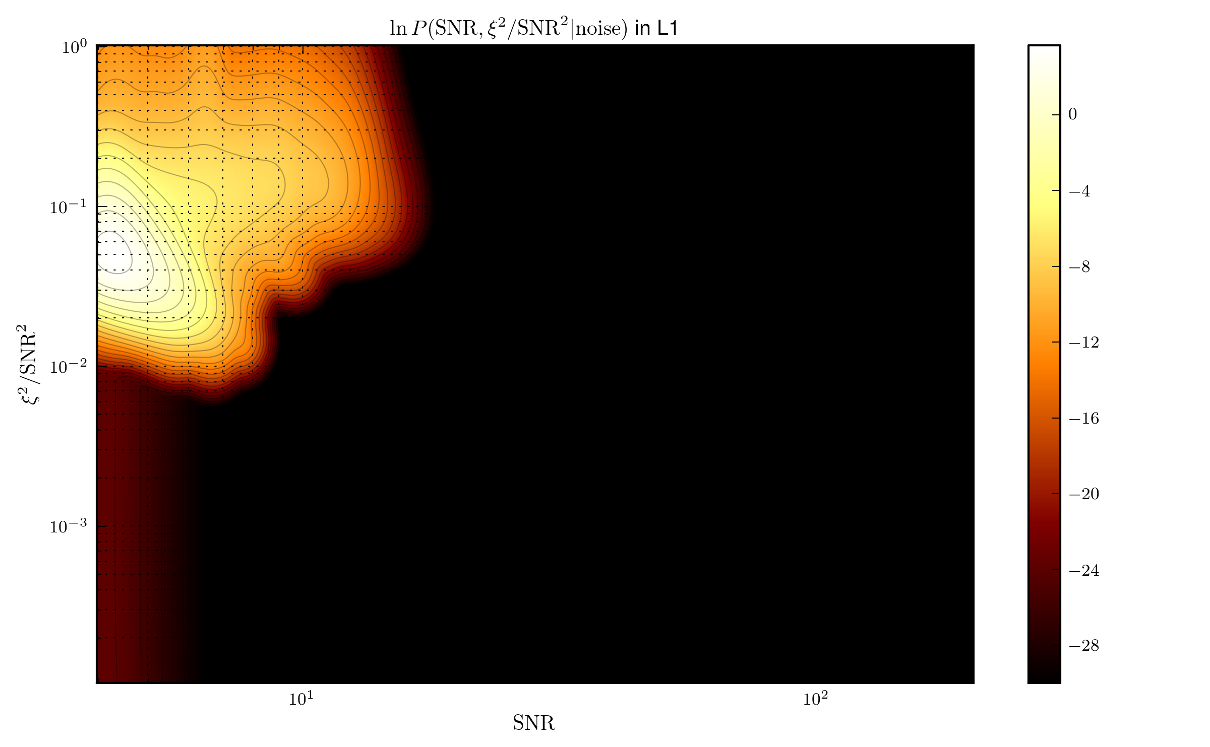
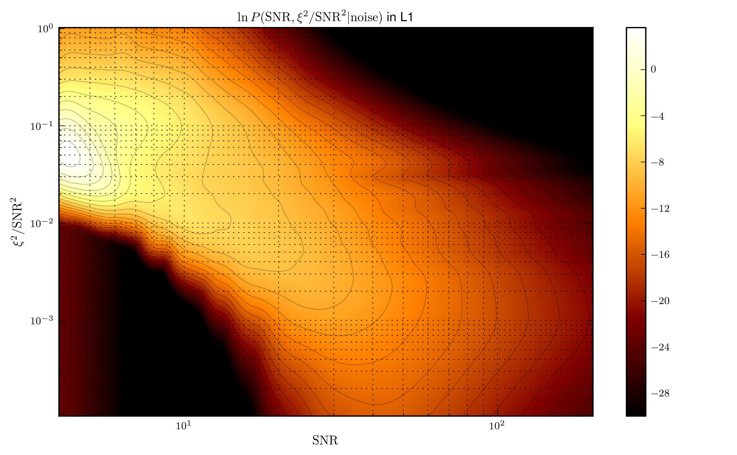
Figure 4: The background PDFs for the same template bank bin using different techniques. Top: the cleanest background PDF we could obtain from the GstLAL inspiral pipeline using original technique since there no injections in the data when estimating the PDF. Middle: the background PDFs obtained from the data with injections using the original technique. Bottom: the background PDFs obtained from the data with injections using improved technique. There is an extended island, which is characteristic of signal-like triggers, filling up the middle figure, but it is not found on the top and bottom figures. This suggests that the characteristic of signal-like triggers is removed by the improved technique and the “true” background is sufficiently restored.

IV.1.3 Discussion

To understand why the technique using the time-reversed template banks is able to improve the the search result, we can examine the differences in the background PDFs between the two techniques. Figure 4 shows three background PDFs for the same region of the parameter space using different techniques. We note that the original data contains no GW signals, so the background PDFs obtained from the original data before adding injections is the cleanest background we could obtain from the GstLAL inspiral pipeline using the original technique. We will refer this background as the optimal background and it is shown on the top of Figure 4. The background PDFs estimated from the data with injections using the original and improved techniques are shown on the middle of Figure 4 and the bottom of Figure 4; they are refered to the contaminated background and the recovered background respectively.

From the contaminated background and optimal background, we can see that the background PDF obtained using the original technique is contaminated by the injections. Any true GW trigger with ($\rho$, $\xi^{2}/\rho^{2}$) value falls into the contaminated region will be penalized by the likelihood-ratio ranking statistic, and tends to be classified as a noise-trigger. The consequence of the contamination is the decrease of the number of events at a given $\text{ln}\mathcal{L}$ threshold (compare Figure 3 : top and Figure 3 : bottom). On the other hand, the recovered background resembles the optimal background but different from the contaminated background. This suggests two results: the improved technique using the time-reversed template bank can estimate the “true” background even though the data is full of injections, and the recovered background can be similar to the optimal background.

The plot of the sensitive volume-time versus the combined FAR (Figure 5) gives a comprehensive comparison of the sensitivity of the pipeline among the three different backgrounds at different FAR thresholds. From the sensitivity plot, we see that the analysis using recovered background is uniformly more sensitive than the contaminated background. This implies that the sensitivity of the search pipeline is greatly improved as a result of this improved technique. On the other hand, the optimal sensitivity is consistent with the sensitivity using the improved technique, sugguesting that the improved technique is able to achieve the optimal sensitivity even in the presence of many injections.

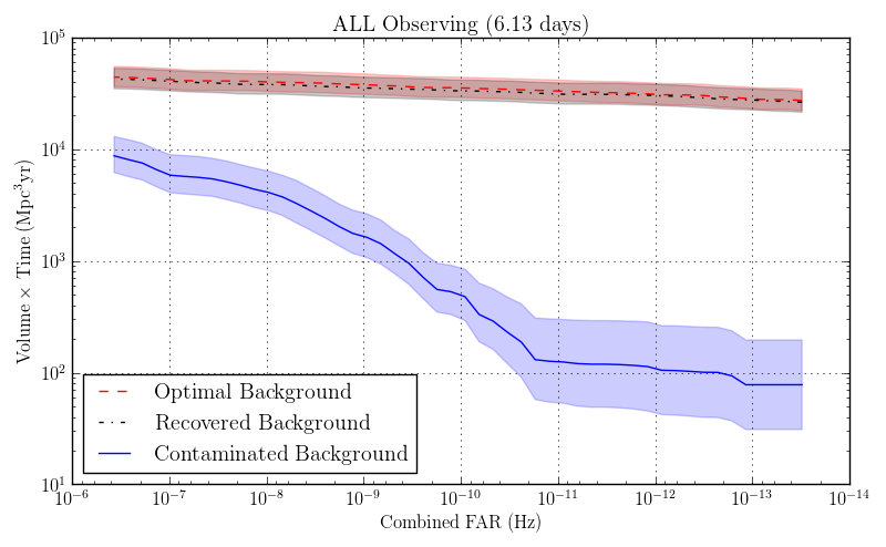
Figure 5: The plot of the sensitive volume-time versus the combined FAR for the three different backgrounds. The sensitivity of the pipeline using the improved technique (with recovered background) is uniformly better than the pipeline using the original technique (with contaminated background). The improved technique is able to achieve the optimal sensitivity in the presence of injections.

IV.2 The Search with Realistic Signals Contamination

The previous results have demonstrated the robustness of the improved background estimation technique in the presence of many signals, we will focus on the performance in the realistic signal contamination in this subsection. In this search, the injection set B (Table 1), which contains three BNS injections in H1 and one BNS injection in L1, were added to the data during the single-detector times. We will continue referring the backgrounds obtained from the original and improved techniques as the contaminated background and recovered background respectively, and the cleanest background that can be obtained by the pipeline is referred to optimal background. They will be used to understand the following search results.

IV.2.1 Search with Optimal Background

Using the optimal background mentioned previously, the search result reveals that Hanford (H1) identified an event occurred roughly at GPS time 1176457885 with $\text{ln}\mathcal{L}=21.7$ and FAR $=4.01\times 10^{-7}$ per second; it is an event that is signficant enough to be considered as recovered. The identification time of this event coincides with one of our injections in H1, which suggests that the pipeline can only recover at most one injection even with the optimal background. The remaining three injections were not identified even in the optimal background because there were not triggers around the injection times, which implies that those injected signals might not be strong enough to be detected or no templates with parameters could match the injections.

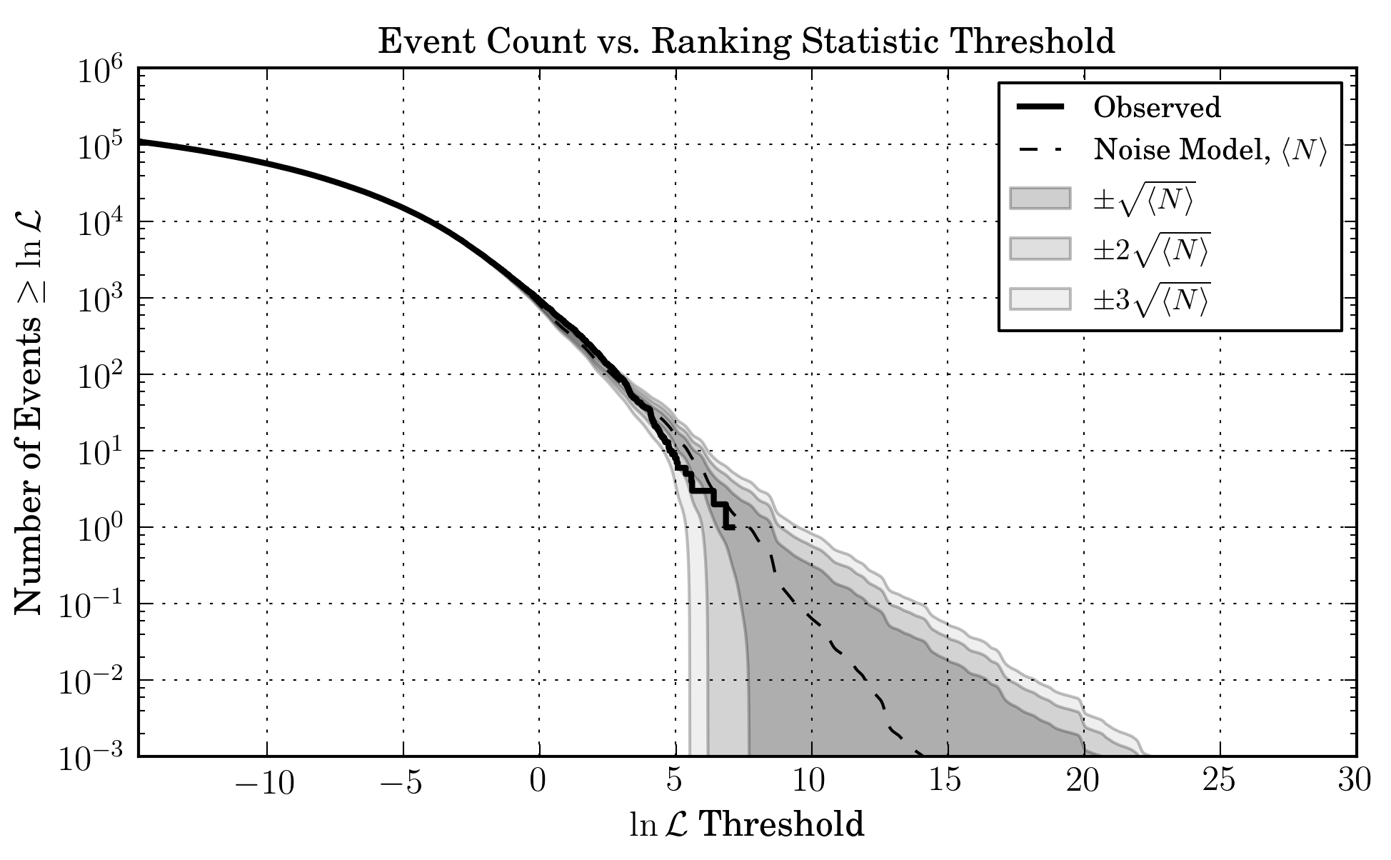
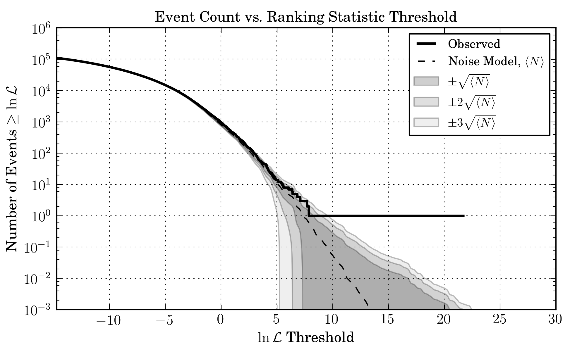
Figure 6: The plots of the event count vs. ranking statistic threshold for the same analysis but using the original technqiue (top) and the improved technique (bottom). There was an injection identified with the improved technique, while there are no injections identified with the original technique.

IV.2.2 Search with Original Background

The search using the contaminated background was not able to identify any event (Figure 6 : top). In particular, the same event is not identified as a significant trigger anymore: it now has $\text{ln}\mathcal{L}=-3.49$ and FAR $=1.00$ per second.

IV.2.3 Search with Improved Background

On the other hand, the search using the recovered background was able to identify the same event with high significance (Figure 6 : bottom). The event is now found with $\text{ln}\mathcal{L}=21.7$ and FAR $=2.62\times 10^{-7}$ per second.

IV.2.4 Discussion

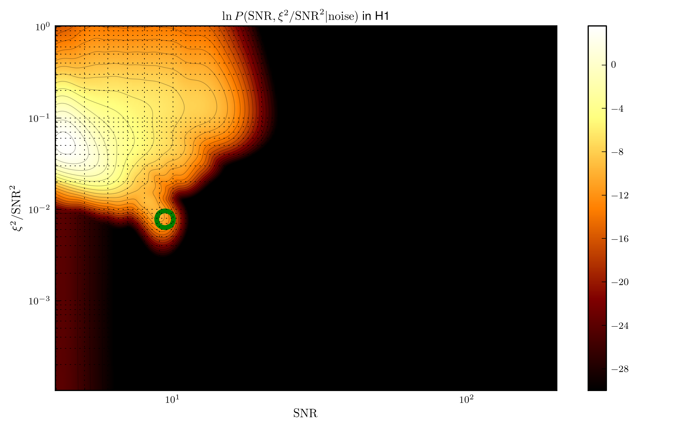
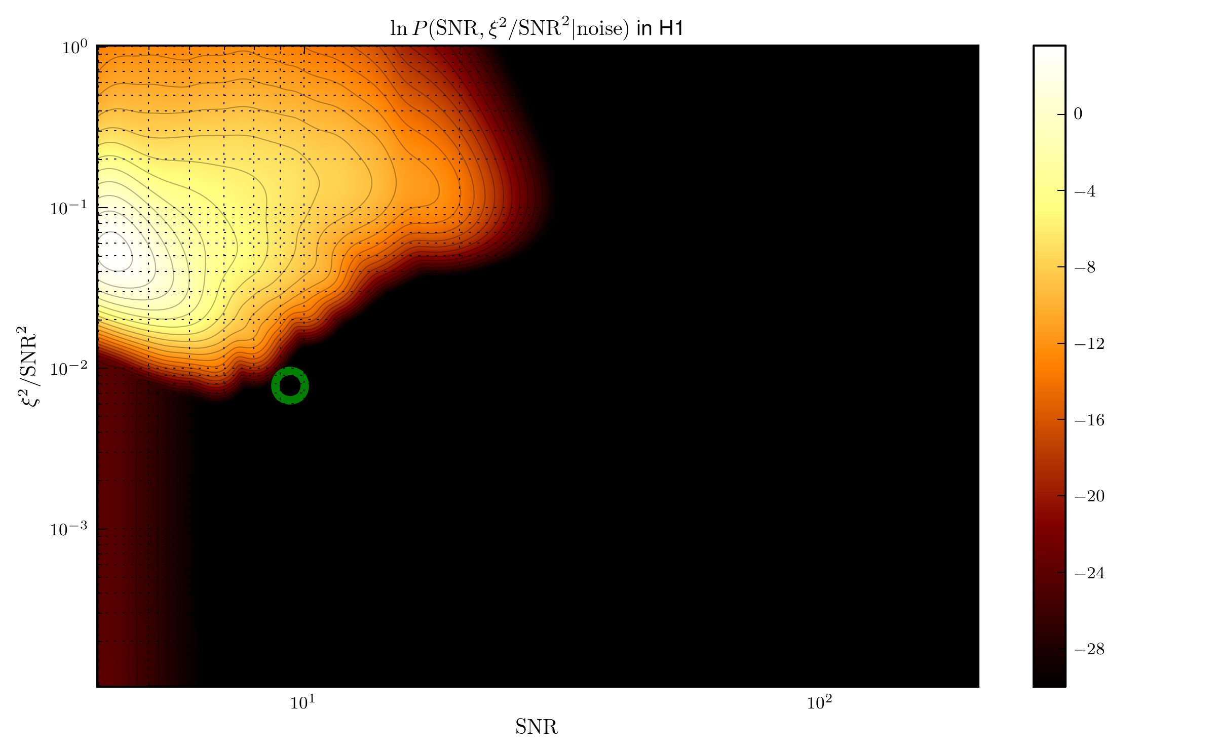
Figure 7: The background PDFs for the same template bank bin using different techniques. The top and bottom figures are the background PDFs obtained from the data with four injections using the original tehcnique and improved technique respectively. There is a small island, which is the contamination due the signal-like triggers, on the top figure, but it is not found on the bottom figure; the green circle is where the location of the identified event on the PDF.

The reason for the original search not being able to identify the event is that the SNR and $\xi^{2}$ values due to that injection were considered as the background samples. This can be seen from the corresponding background ($\rho,\xi^{2}/\rho^{2}$) PDFs: Figure 7. There is an “island” on the top figure (contaminated background PDF) after the 4 injections were added to the data, whereas there was no “island” on the bottom figure (recoverd background PDF).

However, the PDF of the recovered background is extended along SNR axis, suggesting that the statistic of SNR is not properly estimated by the improved method. Nevertheless, for this analysis, it did not show any sign of negative impacts. Finding out the whether the difference will cause any problem for calculating the likelihood ratio, FAP and/or FAR will be left as future works, since the time-reversed template bank has shown its robustness to avoid contamination due to signals.

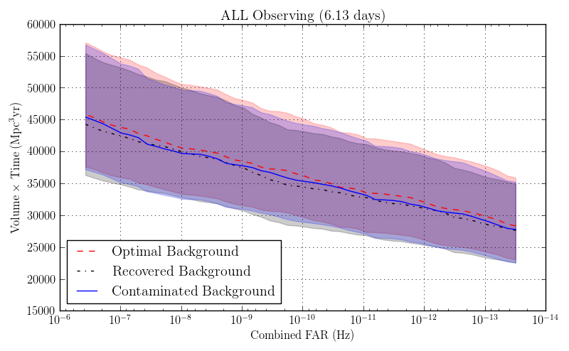
Figure 8: The plot of the sensitive volume-time versus the combined FAR for the three different backgrounds. They are all consistent with each other, suggesting that they are all achieving optimal pipeline sensitivity, suggesting that there are no immediate improvement to the sensitivity in normal signal rate.

The plot of sensitivity is shown on Figure 8. From the figure, there are no significant improvement on the sensitivity and the results from different backgrounds are consistent with each other. This implies that small number of signals cannot deteriorate the sensitivity of the search pipeline (unlike the injection set A). At the present rate of significant triggers observed by GstLAL pipeline (several triggers are recorded into GraceDB with FAR $\leq 3.85\times 10^{-7}$ in a week) gra , the improved background estimation technique might not show immediate improvement to the sensitivity. However, if the background is thought to be contaminated by signals, the improved technique can be used to reveal the uncontaminated background model and assign correct likelihood ratio and FAR.

V Conclusion

We have shown the use of time-reversed template bank to estimate the background model for the searches of GWs from binary neutron star coalescence. We demonstated the improve method with an injection analysis and showed that it can estimate the background model as if it was estimated on the strain data without any signal in presence. However, it is not identically the same, but the search results did not show any sign that they were negatively affected this inaccuracy. Lastly, we demonstrated an application of the new method at a realistic signal rate of one BNS signal per 1.75 days, and showed that it can be used to reveal signals that are originally hidden due to the contamination of background model.