Moment Method for the Boltzmann Equation of Reactive Quaternary Gaseous Mixture

Abstract

We are interested in solving the Boltzmann equation of chemically reacting rarefied gas flows using the Grad’s-14 moment method. We first propose a novel mathematical model that describes the collision dynamics of chemically reacting hard spheres. Using the collision model, we present an algorithm to compute the moments of the Boltzmann collision operator. Our algorithm is general in the sense that it can be used to compute arbitrary order moments of the collision operator and not just the moments included in the Grad’s-14 moment system. For a first-order chemical kinetics, we derive reaction rates for a chemical reaction outside of equilibrium thereby, extending the Arrhenius law that is valid only in equilibrium. We show that the derived reaction rates (i) are consistent in the sense that at equilibrium, we recover the Arrhenius law and (ii) have an explicit dependence on the scalar fourteenth moment, highlighting the importance of considering a fourteen moment system rather than a thirteen one. Through numerical experiments we study the relaxation of the Grad’s-14 moment system to the equilibrium state.

1 Introduction

The Boltzmann equation (BE) accurately models gas flows in all thermodynamic regimes. It governs the evolution of a probability density function that is defined on a seven dimensional space-time-velocity domain. We consider the BE of a gaseous mixture of four mono-atomic gases that react via a chemical reaction given as

$$A_{1}+A_{2}\leftrightarrows A_{3}+A_{4}.$$ (1)

In a concise form, the BE for such a gaseous mixture can be written as

$$d_{t}f_{\alpha}(c_{\alpha},t)=\mathcal{Q}_{\alpha}(f_{1}(c_{1},t),f_{2}(c_{2},t),f_{3}(c_{3},t),f_{4}(c_{4},t)).$$ (2)

Above, $\alpha\in\{1,2,3,4\}$ is an index for the different gases in the mixture, $f_{\alpha}$ represents the probability density function of the $\alpha$-th gas, and $c_{\alpha}\in\mathbb{R}^{3}$ is the molecular velocity. For simplicity, we restrict our study to a spatially homogeneous BE. The collision operator $\mathcal{Q}_{\alpha}$ models the inter-particle interaction and contains contributions from both the chemical and the mechanical interactions. It is noteworthy that a collision between molecules that can undergo a chemical reaction ($A_{1}$ and $A_{2}$, for instance) does not necessarily result in a chemical reaction—the kinetic energy should be large enough to trigger a chemical reaction. Therefore, the part of $\mathcal{Q}_{\alpha}$ that models mechanical collisions contains interactions between all the gas molecules. The explicit form of $\mathcal{Q}_{\alpha}$ discussed later provides further clarification.

We want to solve the above equation using a deterministic method i.e., with a method that does not require Monte-Carlo sampling, which introduces an undesirable stochastic noise in the numerical approximation. We consider a Galerkin type approach where we approximate $f_{\alpha}(\cdot,t)$ in a span of the basis functions $\{\phi_{\alpha,i}\}_{i}$. This provides the approximation

$$f_{\alpha}(\cdot,t)\approx f_{\alpha,N}(\cdot,t)=\sum_{i=0}^{N}\alpha_{i}(t)\phi_{\alpha,i}f_{0}^{\alpha}.$$ (3)

We choose $\phi_{\alpha,i}$ as polynomials in the velocity variable $c_{\alpha}$ and scale them with a Gaussian distribution function $f_{0}^{\alpha}$—the exact form of $\phi_{\alpha,i}$ and $f_{0}^{\alpha}$ is discussed later in section 3. The above approximation was first proposed by Grad [1] and has several desirable properties, it (i) preserves the Galelian invariance of the BE, (ii) results in mass, momentum and energy conservation, (iii) at least in the linearized regime, converges to the BE [2, 3, 4], (iv) results in a hyperbolic moment system under appropriate regularization [5], etc. We refer to the review article [6] and the references therein for an exhaustive discussion.

To compute the approximation $f_{\alpha,N}$, we replace $f_{\alpha}$ by $f_{\alpha,N}$ in the BE, multiply by the test functions $\{\phi_{\alpha,i}\}_{i}$ and integrate over the velocity-domain $\mathbb{R}^{3}$. This results in a time-dependent ordinary-differential-equation (ODE) for the expansion coefficients $\{\alpha_{i}\}_{i}$, or the so-called moment equations. To well-define the moment equations, we need integrals of the form

$$\mathcal{I}_{\alpha}(t):=\int_{\mathbb{R}^{3}}\phi_{\alpha,i}(c_{\alpha},t)\mathcal{Q}_{\alpha}(f_{1}(c_{1},t),f_{2}(c_{2},t),f_{3}(c_{3},t),f_{4}(c_{4},t))dc_{\alpha}.$$ (4)

The main objective of the paper is to compute the above integral. To this end, we study the following three questions related to chemically reactive collisions.

1. Through which molecular potential do the molecules interact?

2. For a given molecular potential and for binary collisions, how to relate the pre and the post collision relative velocities using mass, momentum and energy conservation?

3. For a given relation between the post and the pre collisional relative velocities, how to compute $\mathcal{I}_{\alpha}(t)$?

Note that we only consider the contribution from binary collision in the collision operator $Q_{\alpha}$—a standard assumption in the kinetic gas theory [7]. Furthermore, all the above questions have been extensively studied in the context of mechanical collisions, see [8, 9, 10, 7, 1].

We use the Direction Simulation Monte Carlo (DSMC) method as a motivation to answer the first question and consider a hard sphere interaction potential for both the chemical and the mechanical interactions [11]. Intuitively, the hard sphere potential treats molecules like billiard balls, which interact with each other only when they ”touch” each other. To answer the second question, we assume that the collisions are symmetric that is, the pre collisional relative velocity changes in equal proportions along the normal and the tangential direction of collision. We refer to section 2 for a precise relation between the pre and the post collisional relative velocities. An answer to the third question follows by extending the framework for a mono-atomic binary gas mixture (proposed in [10, 9]) to a mixture of chemically reacting gases.

To the best of our knowledge, only the work in [12] proposes an algorithm to compute the integral $\mathcal{I}_{\alpha}(t)$. It differs from our work in the following sense. Authors in [12] accommodate the chemically reacting molecules at the Maxwell-Boltzmann distribution function corresponding to the thermal equilibrium. This largely simplifies the expression for $\mathcal{I}_{\alpha}(t)$, making the computations simpler. In contrast, we do not make any such assumption. Our framework allows for chemical reactions that occur outside of a thermal equilibrium, which is of particular interest for rarefied gas flows. Here, we emphasis that a thermal equilibrium is different from a chemical equilibrium. In a thermal equilibrium, the probability density function is a Maxwell-Boltzmann distribution function but the number densities do not need to be related by the law of mass action, see [13, 12] or section 4 for details. Furthermore, authors in [12] restrict to a Grad’s-13 approximation i.e., to a particular choice of $N$ in $f_{\alpha,N}$. The framework we propose is not restricted to a particular $N$. However, for demonstration purposes, we focus particularly on the Grad’s-14 approximation.

Let us mention that in DSMC computations, simple scattering models are used to simulate chemically reactive collisions [11]. For instance, see the isotropic variable hard sphere model (VHS) or the anisotropic variable soft sphere model (VSS) [14]. The DSMC literature focuses largely on incorporating effects of preferential dissociation from high-energy internal states into the chemical cross-section models [15]. Moreover, it has been argued that the microscopic details of chemically reactive collisions do not have a significant influence on the flow dynamics [16]. However, to realize/well-define a deterministic method, it is imperative to compute the integral $\mathcal{I}_{\alpha}(t)$, which requires the microscopic details of chemically reactive collisions. Our work proposes one possible way to define these microscopic details.

The BE of chemically reacting gases has not received much attention from a numerical approximation standpoint. Nevertheless, several works in the previous decades have contributed to its theoretical understanding. For the sake of completeness, we briefly recall some of these works. One can show that similar to a single mono-atomic gas, the BE exhibits the H-theorem [17, 18]. Furthermore, the equation has a unique equilibrium that is stable and can be given in terms of the Maxwell-Boltzmann distribution function [18]. Using the Chapman-Enksog expansion, one can also understand the behaviour of the transport coefficients of the gas mixture [19]. Furthermore, with a generalized Chapman–Enksog method, one can provide viscous corrections to the non-equilibrium process rates and study the effect of flow compressibility on the reaction rate coefficients [20, 21].

2 Dynamics of reactive binary collisions

We start with discussing the dynamics of reactive binary collisions. The dynamics of mechanical binary collisions is well studied in the literature [8] and is a special case of reactive collision—details included in remark 2. With $m_{\alpha}$ we denote the mass of the molecule $A_{\alpha}$ and with $\epsilon_{\alpha}$ we denote its energy of formation. We consider chemical reactions of the type $A_{1}+A_{2}\leftrightarrows A_{3}+A_{4}.$ With $\epsilon_{f}$ and $\epsilon_{r}$ we represent the activation energy of the forward and the reverse reaction, respectively. The heat of the reactions is represented by $Q$ and reads

$$Q=\epsilon_{f}-\epsilon_{r}=\left(\epsilon_{3}+\epsilon_{4}\right)-(\epsilon_{1}+\epsilon_{2}).$$

2.1 Mass, momentum and energy conservation

For brevity, we only consider the forward reaction—the relations for the reverse reaction are similar. Throughout the article, we ignore the angular momentum of the molecules. Consider two molecules with masses $m_{1}$ and $m_{2}$ travelling with velocities $c_{1}$ and $c_{2}$, respectively. The molecules collide to form two molecules with masses $m_{3}$ and $m_{4}$, respectively, and with the post collisional velocities $c_{3}$ and $c_{4}$, respectively. We define the pre and the post collisional relative velocities as

$$g_{12}=c_{1}-c_{2},\quad g_{34}=c_{3}-c_{4}.$$ (5)

We assume that $A_{1}$ and $A_{2}$ have enough kinetic energy to trigger a chemical reaction i.e.,

$$\frac{m_{12}g_{12}^{2}}{2}\geq\epsilon_{f},\quad\frac{m_{34}g_{34}^{2}}{2}\geq\epsilon_{r},$$ (6)

where $m_{\alpha\beta}=\frac{m_{\alpha}m_{\beta}}{m_{\alpha}+m_{\beta}}$.

Since mass, momentum and energy are conserved in a binary collision, we find [13]

$$\begin{gathered}m_{1}+m_{2}=m_{3}+m_{4},\quad m_{1}c_{1}+m_{2}c_{2}=m_{3}c_{3}+m_{4}c_{4},\quad\frac{m_{12}|g_{12}|^{2}}{2}=\frac{m_{34}|g_{34}|^{2}}{2}+Q.\end{gathered}$$ (7)

Above, $|\cdot|$ represents the Eucledian norm of a vector. For later convenience, we use the energy balance to derive the following two relations

$$|g_{34}|^{2}=\hat{Q}_{12}g_{12}^{2},\quad|g_{12}|^{2}=\hat{Q}_{34}|g_{34}|^{2},$$ (8)

where

$$\hat{Q}_{12}=\frac{m_{12}}{m_{34}}\left(1-\frac{2Q}{m_{12}g_{12}^{2}}\right),\quad\hat{Q}_{34}=\frac{m_{34}}{m_{12}}\left(1+\frac{2Q}{m_{34}g_{34}^{2}}\right).$$ (9)

Remark 1

The constraint on the kinetic energies to trigger a chemical reaction given in (6) does not take into account the geometry of collision—see [13, 22, 23]. Taking these geometrical effects into account is beyond the scope of the present work and we hope to discuss them in one of our future works.

2.2 Hard sphere interaction potential

With $r_{\alpha\beta}$ we represent the distance between the centres of the two molecules $A_{\alpha}$ and $A_{\beta}$. We assume that these two molecules interact via a molecular potential $\varPsi_{\alpha\beta}\left(r_{\alpha\beta}\right)$ that depends solely on $r_{\alpha\beta}$. We consider a hard sphere interaction potential given as

$$\varPsi_{\alpha\beta}\left(r_{\alpha\beta}\right)=\left\{\begin{array}[]{lr}0&\forall r_{\alpha\beta}>r^{\min}_{\alpha\beta}\\ \infty&\forall r_{\alpha\beta}\leq r^{\min}_{\alpha\beta},\end{array}\right.$$ (12)

where $r_{\alpha\beta}^{\min}$ is the minimum distance between the two molecules. When molecules undergo a mechanical collision, $r_{\alpha\beta}^{\min}$ is the average of the molecular diameters $d_{\alpha}$ and $d_{\beta}$ i.e., $r^{\min}_{\alpha\beta}=\frac{1}{2}\left(d_{\alpha}+d_{\beta}\right).$ For the molecules that undergo a chemical collision, we define $r_{\alpha\beta}^{\min}$ separately for the forward and the reverse reaction as

$$r_{12,f}^{\min}=d_{f},\quad r_{34,r}^{\min}=d_{r}.$$ (13)

Here, $d_{f}$ and $d_{r}$ are the reactive diameters for the forward and the reverse reactions, respectively. Similar to [24], we assume that $d_{f}$ and $d_{r}$ are linearly related to $d_{12}$ and $d_{34}$ in the following way $d_{f}=s_{f}d_{12}$ and $d_{r}=s_{r}d_{34}$, where $s_{f}$ and $s_{r}$ are the so called steric factors—a relation between $s_{f}$ and $s_{r}$ follows from the law of mass action and is given later in (72).

For clarity of the following discussion, we visualize a collision between two hard spheres in Figure 1. The vector $k$ is a unit vector (i.e., $|k|=1$) that passes through the line joining the centres of the two interacting molecules and $b$ is the so-called impact parameter. The angles $\theta$ and $\chi$ are the angle-of-attack and the scattering angle, respectively.

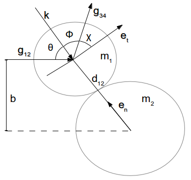
Figure 1: Binary collision for a hard sphere interaction potential. $g_{12}$: relative pre-collisional velocity, $g_{34}$: relative post-collisional velocity, $b$: impact parameter, $k$: a unit vector that passes through the centres of the two colliding spheres, $e_{n}$: normal direction of collision, and $e_{t}$: tangential direction of collision.

2.3 Velocity transformations

The aim of the following discussion is to express the post-collisional velocities $c_{3}$ and $c_{4}$ in terms of the pre-collisional $c_{1}$ and $c_{2}$ ones and vice-versa. We will use these relations later to find the moments of the collision operators given in (2). We start with relating the relative velocity $g_{12}$ to $g_{34}$.

2.3.1 Relating relative velocities: restitution coefficients

Let $e^{n}$ and $e^{t}$ be two orthonormal unit-vectors that define the normal and the tangential direction of collision, respectively. Both of these vectors are shown in Figure 1 and can be related to the vector $k$ via $e^{n}=-k$ and $e^{t}=(-k)_{\bot}$. Let $g_{12}^{n}=\left(g_{12}\cdot e^{n}\right)e^{n}$ and $g_{12}^{t}=\left(g_{12}\cdot e^{t}\right)e^{t}$. Here, $u\cdot v$ represents an Eucledian inner-product between two vectors $u$ and $v$. Similarly, define $g_{34}^{n}$ and $g_{34}^{t}$. Since the span of $e^{n}$ and $e^{t}$ approximates every vector in the collision plan, using the orthogonality of $e^{n}$ and $e_{t}$, we find

$$g_{12}=g_{12}^{n}+g_{12}^{t},\quad g_{34}=g_{34}^{n}+g_{34}^{t}.$$ (14)

Let $\mathcal{E}_{n}$ and $\mathcal{E}_{t}$ be the coefficients of restitution along the normal and the tangential direction, respectively, defined as

$$g^{n}_{34}=\mathcal{E}_{n}g^{n}_{12},\quad g^{t}_{34}=\mathcal{E}_{t}g^{t}_{12}.$$ (15)

We want to find a relation for $\mathcal{E}_{n}$ and $\mathcal{E}_{t}$ in terms of the pre/post collisional velocities $g_{12}/g_{34}$ and the heat of the reaction $Q$. One possibility is to use the Hertzian contact theory of rough inelastic hard spheres [25]. However, involvement of chemical reactions makes the application of Hertzian contact theory complicated and, as yet, it is unclear how to extend this contact theory to chemically reacting molecules. In the present work, we propose to compute $\mathcal{E}_{n}$ and $\mathcal{E}_{t}$ by assuming that the pre-collisional relative velocity $g_{12}$ changes in equal proportions along the normal and the tangential direction of collision. Equivalently,

$$\mathcal{E}_{n}=\mathcal{E}_{t}=\mathcal{E}.$$ (16)

To compute $\mathcal{E}$, we first note that $|g_{34}|^{2}=\mathcal{E}^{2}|g_{12}|^{2}$. Then, the energy balance given in (8) provides

$$\mathcal{E}=\sqrt{\hat{Q}_{12}}.$$ (17)

Note that we have only considered the positive root in the above expression because $\mathcal{E}_{n}$ cannot be negative. Also note that $\hat{Q}_{12}\geq 0$ because of the constraint on the kinetic energy (6).

We elaborate on the above assumption (16). A collision between chemically reactive molecules results in a destruction or a formation of chemical bonds. This results in (i) exchange of reaction heat that is quantified by $Q$, and (ii) a change in mass of the interacting molecules. As per the above assumption, both these effects influence the pre collisional relative velocity $g_{12}$ equally along the normal and the tangential direction of collision. Equivalently, there is no preferred direction of motion along which a chemical reaction changes the pre-collisional relative velocity differently.

A collision between two rough inelastic hard spheres also results in a change in both the tangential and the normal pre-collisional relative velocity. We discuss the differences of our collision model to the collision model of a rough inelastic hard sphere. We refer to [26] for a detailed discussion on a rough inelastic hard sphere.

1. For an inelastic rough hard sphere, two different mechanisms change the pre-collisional relative velocity—friction changes the tangential velocity and the inelasticity changes the normal velocity. Since both these mechanisms are different, usually, $\mathcal{E}_{n}\neq\mathcal{E}_{t}$. In contrast, for a chemically reactive collision, a single mechanism—the chemical reaction—is responsible for a change in both the normal and the tangential pre-collisional velocity, which motivates our assumption $\mathcal{E}_{n}=\mathcal{E}_{t}$.

2. For a rough inelastic hard sphere, if the friction is sufficiently large then $\mathcal{E}_{t}$ can be negative, resulting in a change in both the tangential and the normal pre-collisional velocity. In our model $\mathcal{E}_{t}$ is positive thus, the pre-collisional relative velocity can only change in magnitude.

2.3.2 Relating pre and post collisional velocities

We now express $c_{3}/c_{4}$ in terms of $c_{1}/c_{2}$. We first summarise our results, and devote the rest of the discussion in proving it. The post-collisional velocities $c_{3/4}$ are related to the pre-collisional ones $c_{1/2}$ via

$$c_{3}=c_{1}+g_{12}\left(\mu_{43}\sqrt{\hat{Q}_{12}}-\mu_{21}\right)-2\mu_{43}\sqrt{\hat{Q}_{12}}\left(k\cdot g_{12}\right)k,$$ (18)

$$c_{4}=c_{2}-g_{12}\left(\mu_{34}\sqrt{\hat{Q}_{12}}-\mu_{12}\right)+2\mu_{34}\sqrt{\hat{Q}_{12}}\left(k\cdot g_{12}\right)k.$$ (19)

Above, $k$ is the unit vector shown in Figure 1 and $\hat{Q}_{12}$ is as given in (8). Furthermore, $\mu_{\alpha\beta}$ is the mass fraction defined as

$$\mu_{\alpha\beta}=m_{\alpha}/(m_{\alpha}+m_{\beta}).$$ (20)

Expressions for $c_{1}$ and $c_{2}$ can be derived in a similar fashion and are given as

$$c_{1}=c_{3}+g_{34}\left(\mu_{21}\sqrt{\hat{Q}_{34}}-\mu_{43}\right)+2\mu_{21}\sqrt{\hat{Q}_{34}}\left(k\cdot g_{34}\right)k,$$ (21)

$$c_{2}=c_{4}-g_{34}\left(\mu_{12}\sqrt{\hat{Q}_{34}}-\mu_{34}\right)-2\mu_{12}\sqrt{\hat{Q}_{34}}\left(k\cdot g_{34}\right)k.$$ (22)

We now derive the above relations. First recall that the angles $\theta$, $\phi$ and $\chi$ are as shown in Figure 1. Since we assume that the collision is symmetric (i.e., (16) holds) we find that (i) $\theta=\phi$, (ii) $\chi=\pi-2\theta$, and (iii) $k$ is a vector that bisects $g_{12}$ and $g_{34}$ and is given as

$$k=\frac{\left(\sqrt{\hat{Q}_{12}}g_{12}-g_{34}\right)}{\left|\sqrt{\hat{Q}_{12}}g_{12}-g_{34}\right|}.$$ (23)

Taking a dot product of the above equation with $\sqrt{\hat{Q}_{12}}g_{12}-g_{34}$, we obtain the following relation

$$k\cdot\left(\sqrt{\hat{Q}_{12}}g_{12}-g_{34}\right)=\left|\sqrt{\hat{Q}_{12}}g_{12}-g_{34}\right|$$ (24)

Since $k$ bisects $g_{12}$ and $g_{34}$, we also have

$$k\cdot g_{34}=-|g_{34}|\cos(\phi)=-\sqrt{\hat{Q}_{12}}|g_{12}|\cos(\theta)=-\sqrt{\hat{Q}_{12}}k\cdot g_{12}.$$ (25)

Substituting (25) into (24) we have

$$\left|\sqrt{\hat{Q}_{12}}g_{12}-g_{34}\right|=2\sqrt{\hat{Q}_{12}}k\cdot g_{12}$$ (26)

Substituting the above relation into the definition of $k$ given in (23) we have

$$g_{34}=\sqrt{\hat{Q}_{12}}g_{12}-2\sqrt{\hat{Q}_{12}}\left(k\cdot g_{12}\right)k.$$ (27)

The velocity of the center of mass of the system, namely $h$, is given as

$$h=\mu_{12}c_{1}+\mu_{21}c_{2}=\mu_{34}c_{3}+\mu_{43}c_{4}$$ (28)

Note that the second equality is a result of the momentum conservation given in (7). Using the center of mass velocity $h$ and the post collisional relative velocity $g_{34}$, the post-collisional velocities $c_{3}$ and $c_{4}$ can be written as

$$c_{3}=h+\mu_{43}g_{34}\quad c_{4}=h-\mu_{34}g_{34},$$ (29)

which is equivalent to

$$c_{3}=\mu_{12}c_{1}+\mu_{21}c_{2}+\mu_{43}g_{34},\quad c_{4}=\mu_{12}c_{1}+\mu_{21}c_{2}-\mu_{34}g_{34}.$$ (30)

Finally, using (27) in the above expression, we express $g_{34}$ in terms of $g_{12}$ to find the desired result.

Remark 2

For consistency, we show that the velocity transformations for a single mono-atomic gas and a binary mixture of (chemically neutral) mono-atomic gases follow from the velocity transformations of a chemically reactive gas mixture. For a single gas and for all $\alpha\in\{1,2,3,4\}$, we have $m_{\alpha}=m$ and $Q=0$. As a result, the velocity transformations (18)–(22), change to $c_{3}=c_{1}-\left(k\cdot g_{12}\right)k$ and $c_{4}=c_{2}+\left(k\cdot g_{12}\right)k$. For a binary mixture, we have $m_{1}=m_{3},$ $m_{2}=m_{4},$ and $Q=0$. Using these physical parameters, the velocity transformations change to $c_{3}=c_{1}-2\mu_{21}\left(k\cdot g_{12}\right)k$ and $c_{4}=c_{2}+2\mu_{12}\left(k\cdot g_{12}\right)k$. One can easily check that these relations are the same as those given in [8, 9].

3 Moment Approximation

We present our moment approximation for the BE given in (2). We start with giving the explicit form of the collision operator appearing in the BE (2).

3.1 Collision operator

We split the collision operator $\mathcal{Q}_{\alpha}$ as

$$\mathcal{Q}_{\alpha}(f_{1},f_{2},f_{3},f_{4})=\sum_{\beta=1}^{4}\mathcal{Q}_{M}(f_{\alpha},f_{\beta})+\mathcal{Q}_{\alpha,R}(f_{1},f_{2},f_{3},f_{4}).$$ (31)

Above, $\mathcal{Q}_{M}(f_{\alpha},f_{\beta})$ models the mechanical collisions between $A_{\alpha}$ and $A_{\beta}$, and $\mathcal{Q}_{\alpha,R}$ models the chemically reactive collisions. The expression for $\mathcal{Q}_{M}$ is the same as that for a single gas and reads [8]

$$\mathcal{Q}_{M}(f_{\alpha},f_{\beta})=\int_{\mathbb{R}^{3}}\int^{2\pi}_{0}\int_{0}^{\pi}\left(f_{\alpha}^{{}^{\prime}}f^{{}^{\prime}}_{\beta}-f_{\alpha}f_{\beta}\right)g_{\alpha\beta}\sigma_{\alpha\beta}\sin(\chi)d\chi d\epsilon dc_{\beta},$$ (32)

where $f_{\alpha}^{^{\prime}}$ and $f_{\beta}^{{}^{\prime}}$ represent the phase densities corresponding to the post collisional velocities $c_{\alpha}^{{}^{\prime}}$ and $c_{\beta}^{^{\prime}}$, respectively, $\epsilon$ represents the angle made by the collisional plane, and $\sigma_{\alpha\beta}$ represents the differential cross-section. For a hard sphere interaction potential, $\sigma_{\alpha\beta}$ is given as [8, 10]

$$\sigma_{\alpha\beta}=\frac{1}{4}d^{2}_{\alpha\beta},\quad d_{\alpha\beta}=\frac{1}{2}(d_{\alpha}+d_{\beta}).$$

The operator $\mathcal{Q}_{\alpha,R}$ that accounts for chemical reactions can be given as [11, 13]

$$\mathcal{Q}_{\alpha,R}(f_{1},f_{2},f_{3},f_{4})dc_{\alpha}= \nu_{\alpha}\int_{\mathbb{R}^{3}}\int_{\mathbb{R}^{3}}\int^{2\pi}_{0}\int_{0}^{\pi}f_{1}f_{2}g_{12}\sigma_{12}^{f}\sin(\chi)d\chi d\epsilon dc_{1}dc_{2}$$ (33)

$$-\nu_{\alpha}\int_{\mathbb{R}^{3}}\int_{\mathbb{R}^{3}}\int^{2\pi}_{0}\int_{0}^{\pi}f_{3}f_{4}g_{34}\sigma_{34}^{r}\sin(\chi)d\chi d\epsilon dc_{3}dc_{4},$$

where $\nu_{\alpha}$ is a stoichiometric coefficient given as $-\nu_{1}=-\nu_{2}=\nu_{3}=\nu_{4}=1.$ Furthermore, $\sigma_{12}^{f}$ and $\sigma_{34}^{r}$ are the differential cross-sections corresponding to the forward and the reverse reaction, respectively. For a hard sphere interaction potential, both these cross-sections read

$$\sigma_{12}^{f}= U\left(1-\frac{2\epsilon_{f}}{m_{12}g_{12}^{2}}\right)\frac{d_{f}^{2}}{4}\left(1-\frac{2\epsilon_{f}}{m_{12}g_{12}^{2}}\right),$$ (34)

$$\sigma_{34}^{r}= U\left(1-\frac{2\epsilon_{r}}{m_{34}g_{34}^{2}}\right)\frac{d_{r}^{2}}{4}\left(1-\frac{2\epsilon_{r}}{m_{34}g_{34}^{2}}\right).$$ (35)

Above, $U(x)$ is a unit-step function that is one for $x\geq 0$ and zero otherwise. Furthermore, $d_{f}$ and $d_{r}$ are as given in (13).

3.2 Definition of moments

Let $i\in\mathbb{R}^{N}$ denote a multi-index with each entry being a natural number smaller than the velocity space dimension $d$. Using $i$ and a scalar $a\in\mathbb{N}$, we define a polynomial over $\mathbb{R}^{d}$ as

$$\phi_{a,\langle i_{1}\dots i_{N}\rangle}(y)=|y|^{2a}y_{\langle i_{1}}\dots y_{i_{N}\rangle},\quad y\in\mathbb{R}^{d}.$$ (36)

The tensor $y_{\langle i_{1}}\dots y_{i_{N}\rangle}$ represents the trace free part of $y_{i_{1}}\cdots y_{i_{N}}$ and its explicit form can be found in [7]. For completeness, we give this explicit form for $N=2$

$$B_{\langle i_{1}i_{2}\rangle}=\frac{1}{2}\left(B_{i_{1}i_{2}}+B_{i_{2}i_{1}}\right)-\frac{1}{3}\delta_{i_{1}i_{2}}B_{i_{k}i_{k}},$$ (37)

where $\delta_{i_{1}i_{2}}$ is a Kronecker delta. Throughout the article, we use the Einstein’s summation convention for the tensor notation.

Using $\phi_{a,\langle i_{1}\dots i_{N}\rangle}$, we define a general $(2a+N)$-th order moment of $f_{\alpha}$ as

$$w^{\alpha}_{a,i_{1}\dots i_{N}}(t)=m_{\alpha}\int_{\mathbb{R}^{d}}\phi_{a,\langle i_{1}\dots i_{N}\rangle}(C_{\alpha})f_{\alpha}(c_{\alpha},t)dC_{\alpha}.$$ (38)

Above, $C_{\alpha}$ is the so-called peculiar velocity given as $C_{\alpha}=c_{\alpha}-v$. Here, $v$ is the macroscopic velocity of the gas mixture defined in the following way. Let the density $\rho_{\alpha}$ and the macroscopic velocity $v_{\alpha}$ of gas-$\alpha$ be defined as

$$\rho_{\alpha}=w^{\alpha}_{0,0},\quad\rho_{\alpha}v^{\alpha}_{i_{1}}=w^{\alpha}_{0,i_{1}}.$$ (39)

We define the mixture velocity $v$ and the mixture density $\rho$ as

$$\rho=\sum_{\alpha=1}^{4}\rho_{\alpha},\quad\rho v=\sum_{\alpha=1}^{4}\rho_{\alpha}v_{\alpha}.$$ (40)

The other moments of $f_{\alpha}$ that have a physical relevance are given as

$$\begin{gathered}\frac{3}{2}kT_{\alpha}=\frac{3}{2}\rho_{\alpha}\theta_{\alpha}=\frac{1}{2}w^{\alpha}_{1,0}\quad\sigma_{i_{1}i_{2}}^{\alpha}=w^{\alpha}_{0,i_{1}i_{2}},\quad q^{\alpha}_{i_{1}}=\frac{1}{2}w^{\alpha}_{1,i_{1}}.\end{gathered}$$ (41)

Above, $\theta_{\alpha}=kT_{\alpha}/m_{\alpha}$ is the temperature in energy units with $k$ being the Boltzmann’s constant, $\sigma_{i_{1}i_{2}}^{(\alpha)}$ is the stress-tensor and $q^{(\alpha)}_{i_{1}}$ is the heat flux. For convenience, we further define

$$\Delta_{\alpha}=w^{\alpha}_{2,0}-15\rho_{\alpha}\theta_{\alpha}^{2}.$$

We also define the temperature $\theta$ and the number density $n$ of the gas mixture as

$$kT=\rho\theta=\sum_{i=1}^{4}\rho_{\alpha}\theta_{\alpha},\quad n=\sum_{i=1}^{4}n_{\alpha},$$

where $n_{\alpha}=\rho_{\alpha}/m_{\alpha}$.

Remark 3

Note that due to mass, momentum and energy conservation, the mixture velocity $v$ is constant over time resulting in a time-independent peculiar velocity $C_{\alpha}$.

3.3 The fourteen moment system

We are interested in solving for only the $14$ moments contained in the set

$$w_{\alpha}^{[14]}=\{w^{\alpha}_{0,0},w^{\alpha}_{0,i_{1}},\frac{1}{2}w^{\alpha}_{1,0},w^{\alpha}_{0,i_{1}i_{2}},\frac{1}{2}w^{\alpha}_{1,i_{1}},w^{\alpha}_{2,0}\}.$$

Note that as per the above relations, this set contains one component for $\rho_{\alpha}$, three for $v_{\alpha}$, one for $\theta_{\alpha}$, six for $\sigma_{\alpha}$, three for $q_{\alpha}$ and one for $w^{\alpha}_{2,0}$—thus fourteen in total. Given the moment vector $w_{\alpha}^{[14]}$, we first want to approximate the distribution function $f_{\alpha}$. We consider the Grad’s-14 (G14) moment approximation and approximate $f_{\alpha}$ by [1, 26]

$$f_{\alpha}\approx f_{\alpha|G14}=f_{0}^{\alpha}\left[1+\frac{\Delta_{\alpha}}{8\rho_{\alpha}\theta_{\alpha}^{2}}\left(1-\frac{2}{3}\frac{|C_{\alpha}|^{2}}{\theta_{\alpha}}+\frac{1}{15}\frac{|C_{\alpha}|^{4}}{\theta_{\alpha}^{2}}\right)+\frac{q^{(\alpha)}_{i_{1}}C^{(\alpha)}_{i_{1}}}{5\rho_{\alpha}\theta_{\alpha}^{2}}\left(\frac{|C_{\alpha}|^{2}}{\theta_{\alpha}}-5\right)\right.$$

$$\left.+\frac{\sigma_{i_{1}i_{2}}^{(\alpha)}}{2\rho_{\alpha}\theta_{\alpha}^{2}}C_{i_{1}}^{(\alpha)}C_{i_{2}}^{(\alpha)}+\frac{u^{(\alpha)}_{i_{1}}C^{(\alpha)}_{i_{1}}}{\theta_{\alpha}}\right].$$ (42)

The function $f_{0}^{\alpha}$ is a Gaussian-distribution function defined as

$$f_{0}^{\alpha}=n_{\alpha}\left(\frac{1}{2\pi\theta_{\alpha}}\right)^{\frac{d}{2}}\exp\left(-\frac{|C_{\alpha}|^{2}}{2\theta_{\alpha}}\right).$$ (43)

To derive a governing equation for the moments $w_{\alpha}^{[14]}$, we replace $f_{\alpha}$ by $f_{\alpha|G14}$ in the BE (2), multiply the resulting equation by appropriate functions $\phi_{a,\langle i_{1}\dots i_{N}\rangle}(C_{\alpha})$ and integrate over the velocity domain $\mathbb{R}^{d}$. For all $\alpha\in\{1,2,3,4\}$, this results in the moment equations

$$\begin{gathered}d_{t}n_{\alpha}=\mathcal{P}^{\alpha}_{R,0},\quad d_{t}\left(n_{\alpha}v^{\alpha}_{i_{1}}\right)=\mathcal{P}^{\alpha}_{M,i_{1}}+\mathcal{P}^{\alpha}_{R,i_{1}},\\ \frac{3}{2}d_{t}(n_{\alpha}T_{\alpha})=\mathcal{P}^{\alpha}_{M,1}+\mathcal{P}^{\alpha}_{R,1},\quad d_{t}\sigma^{(\alpha)}_{i_{1}i_{2}}=\mathcal{P}^{\alpha}_{M,i_{1}i_{2}}+\mathcal{P}^{\alpha}_{R,i_{1}i_{2}},\\ d_{t}q^{(\alpha)}_{i_{1}}=\mathcal{P}^{\alpha}_{M,1,i_{1}}+\mathcal{P}^{\alpha}_{R,1,i_{1}},\quad d_{t}u^{2(\alpha)}=\mathcal{P}^{\alpha}_{M,2}+\mathcal{P}^{\alpha}_{R,2}.\end{gathered}$$ (44)

The different $\mathcal{P}^{\alpha}$’s are the moments of the collision operator defined as

$$\mathcal{P}^{\alpha}_{M,a,i_{1}\dots i_{N}}= m_{\alpha}\sum_{\beta=1}^{4}\int_{\mathbb{R}^{d}}\phi_{a,\langle i_{1}\dots i_{N}\rangle}Q_{M}(f_{\alpha|G14},f_{\beta|G14})dC_{\alpha},$$ (45)

$$\mathcal{P}^{\alpha}_{R,a,i_{1}\dots i_{N}}= m_{\alpha}\int_{\mathbb{R}^{d}}\phi_{a,\langle i_{1}\dots i_{N}\rangle}Q_{\alpha,R}(f_{1|G14},f_{2|G14},f_{3|G14},f_{4|G14})dC_{\alpha}.$$

Above, $Q_{M}$ and $Q_{\alpha,R}$ are the mechanical and the chemical parts of the collision operator given in (31). Note that the mechanical collisions do not contribute into the mass balance equation.

Remark 4

Strictly speaking, the Grad’s-14 moment approximation is a special case of the approximation $f_{\alpha|G14}$ given in (42). In $f_{0}^{\alpha}$, if we replace the ”local” gas temperature $\theta_{\alpha}$ by the temperature of the mixture $\theta$, we find the Grad’s-14 moment approximation. We expect $f_{\alpha|G14}$ to be more accurate than a Grad’s-14 moment approximation because it adapts better to the changes in the ”local” temperature of the gas-$\alpha$.

Remark 5

The following two observations motivate our choice of a fourteen moment system rather than a thirteen one. Firstly, out of all the fourteen moments, only the non-equilibrium moment $\Delta_{\alpha}$ (and not the stress tensor and the heat flux) influences the reaction rates, which can result in a better approximation of the reaction rates outside of the equilibrium—see (66) and (67) derived later for explicit reaction rates. We emphasise that for a thirteen moment system, none of the non-equilibrium moments will appear in the reaction rates. Secondly, as discussed earlier, we treat a chemically reacting mixture similar to a granular gas in the sense that we allow both the normal and the tangential pre-collisional velocities to change. Previous works have shown that including $\Delta_{\alpha}$ in the set of moments better captures the cooling rate and the transport coefficients of a granular gas [26, 27]. We expect a similar result to hold true for a chemically reactive mixture. Our numerical experiments corroborate our expectations by demonstrating that non-equilibrium states where $\Delta_{\alpha}$ is initially zero can trigger non-zero perturbations in $\Delta_{\alpha}$, while all the other non-equilibrium moments remain zero.

3.4 Moments of the collision operator

To compute the moments of $\mathcal{Q}_{M}$ we first derive moments of $\mathcal{Q}_{\alpha,R}$ and interpret the mechanical collisions as a special case of the chemical collisions by using the physical parameters given in remark 2. This results in the same moments as those given in [9, 10]. For brevity, we do not discuss these moments here again.

To compute the moments of $\mathcal{Q}_{\alpha,R}$, we restrict ourselves to $\alpha=1$, since computations for all the other gas components are the same. First, we decompose $\mathcal{Q}_{1,R}$ into a gain $\mathcal{Q}^{g}_{1,R}$ and a loss part $\mathcal{Q}^{f}_{1,R}$ as

$$\mathcal{Q}_{1,R}(f_{1|G14},f_{2|G14},f_{3|G14},f_{4|G14})dC_{1}= \underbrace{\int f_{3|G14}f_{4|G14}g_{34}\sigma_{34}^{r}\sin(\chi)d\chi d\epsilon dC_{3}dC_{4}}_{\mathcal{Q}_{g}dC_{1}}$$ (46)

$$\underbrace{-\int f_{1|G14}f_{2|G14}g_{12}\sigma_{12}^{r}\sin(\chi)d\chi d\epsilon dC_{1}dC_{2}}_{=\mathcal{Q}_{l}dC_{1}}.$$

It is easy to conclude that $\mathcal{Q}_{g}$ and $\mathcal{Q}_{l}$ results in a gain and a loss in $f_{1}$, respectively. Note that because $f_{1|G14}$ is expressed in terms of $C_{1}$, we have changed the integration variable from $c_{1}$ to $C_{1}$. To perform the change we have used the relation $dc_{1}=dC_{1}$, which immediately follows from the definition of $C_{1}$.

To simplify the following notations, rather than computing the moments of $\mathcal{Q}_{\alpha,R}$ with respect to the polynomial $\phi_{a,\langle i_{1}\dots i_{N}\rangle}$ given in (36), we compute the moments with respect to the monomial $\phi_{i_{1}\dots i_{N}}$ defined as

$$\phi_{i_{1}\dots i_{N}}(C_{\alpha})=C_{i_{1}}^{\alpha}\dots C_{i_{N}}^{\alpha}.$$ (47)

Using the definition of $C_{\langle i_{1}}\dots\cdot C_{i_{N}\rangle}$ and expressing $|C_{\alpha}|^{2a}$ in terms of the different components of $C_{\alpha}$, one can conclude that for any $a\in\mathbb{N}$, the function $\phi_{a,\langle i_{1}\dots i_{N}\rangle}(C_{\alpha})$ can be recovered via linear combinations of $\phi_{i_{1}\dots i_{N}}(C_{\alpha})$, making it straightforward to express $\int_{\mathbb{R}^{d}}\phi_{a,\langle i_{1}\dots i_{N}\rangle}\mathcal{Q}_{\alpha,R}dC_{\alpha}$ in terms of $\int_{\mathbb{R}^{d}}\phi_{i_{1}\dots i_{N}}\mathcal{Q}_{\alpha,R}dC_{\alpha}$.

We define the moments of $\mathcal{Q}_{g}$ and $\mathcal{Q}_{l}$ with respect to $\phi_{i_{1}\dots i_{N}}(C_{1})$ as

$$\mathcal{P}^{g}_{i_{1}\dots i_{N}}= m_{1}\int\phi_{i_{1}\dots i_{N}}(C_{1})\mathcal{Q}_{g}dC_{1}=m_{1}\int\phi_{i_{1}\dots i_{N}}(C_{1})f_{3|G14}f_{4|G14}g_{34}\sigma_{34}^{r}\sin(\chi)d\chi d\epsilon dC_{3}dC_{4},$$ (48)

$$\mathcal{P}^{l}_{i_{1}\dots i_{N}}= m_{1}\int\phi_{i_{1}\dots i_{N}}(C_{1})\mathcal{Q}_{l}dC_{1}=-m_{1}\int\phi_{i_{1}\dots i_{N}}(C_{1})f_{1|G14}f_{2|G14}g_{12}\sigma_{12}^{f}\sin(\chi)d\chi d\epsilon dC_{1}dC_{2}.$$

Above, for brevity we have represented all the integrals with a single integration symbol. To compute $\mathcal{P}^{g}_{i_{1}\dots i_{N}}$, we follow the steps outlined in algorithm 1—the details of the algorithm are given thereafter. In the first step, we express $\phi_{i_{1}\dots i_{N}}(C_{1})$ in terms of the integration variables $C_{3}$ and $C_{4}$. To compute $\mathcal{P}^{l}_{i_{1}\dots i_{N}}$, this transformation is not needed. All the other steps remain the same as that for $\mathcal{P}^{g}_{i_{1}\dots i_{N}}$ therefore, we only discuss the computation of $\mathcal{P}^{g}_{i_{1}\dots i_{N}}$. Note that the production terms resulting from algorithm 1 are included in the supplementary material.

Algorithm 1 Algorithm to compute $\mathcal{P}^{g}_{i_{1}\dots i_{N}}$

1:  Using the velocity transformations outlined in subsection 2.3, express $\phi_{i_{1}\dots i_{N}}(C_{1})$ in terms of $C_{3}$ and $C_{4}$.

2:  Perform integration over the angles that determine the collision orientation i.e., the angles $\chi$ and $\epsilon$ appearing in (48). This results in an integral over $C_{3}$ and $C_{4}$.

3:  Define new integration variables in terms of $C_{3}$ and $C_{4}$ such that the integral in the previous step can be written in terms of two separate integrals, with each integral expressed solely in terms of a single integration variable.

4:  With a method-of-choice, perform integration over the two separate integrals resulting from the previous step. We use the symbolic integration from mathematica to compute these integrals.

Remark 6

Note that algorithm 1 can be used to compute an arbitrary order moment of the collision operator and not just the fourteen moments. However, for the sake of demonstration, during numerical experiments and in the production terms outlined in the supplementary material, we stick to the Grad’s-14 moment approximation.

3.4.1 Step-1: Transformation of the test function

Let $\varpi_{1}=\mu_{21}\sqrt{\hat{Q}_{34}}$, where $\mu_{21}$ is the mass fraction defined in (20) and $\hat{Q}_{34}$ is as given in (8). We express the velocity transformations given in (21) as

$$C^{(1)}_{i_{r}}=C^{(3)}_{i_{r}}+(\varpi_{1}-\mu_{43})g^{(34)}_{i_{r}}-2\varpi_{1}g_{34}\cos\theta k_{i_{r}}\quad(\because k\cdot g_{12}=|g_{12}|\cos(\theta)).$$ (49)

Let $d=(\varpi_{1}-\mu_{43})g_{34}-2k\varpi_{1}|g_{34}|\cos\theta$. Then, the monomial $\phi_{i_{1}\dots i_{N}}$ given in (47) can be expressed as

$$\phi_{i_{1}\dots i_{N}} =m_{1}(C^{(3)}_{i_{1}}+d_{i_{1}})(C^{(3)}_{i_{2}}+d_{i_{2}})(C^{(3)}_{i_{3}}+d_{i_{3}})\dots(C^{(3)}_{i_{N}}+d_{i_{N}}),$$

$$=m_{1}\sum_{\beta_{1}=0}^{N}{{N}\choose{\beta_{1}}}d_{({i_{1}}}d_{i_{2}}d_{i_{3}}\dots d_{i_{\beta_{1}}}C^{(3)}_{i_{\beta_{1}+1}}\dots C^{(3)}_{{i_{N}})}.$$ (50)

We simplify $d_{{i_{1}}}d_{i_{2}}d_{i_{3}}\dots d_{i_{\beta_{1}}}$ as

$$d_{i_{1}}d_{i_{2}}\dots d_{i_{\beta_{1}}} =((\varpi_{1}-\mu_{43})g^{(34)}_{i_{1}}-2\varpi_{1}g_{34}\cos\theta k_{i_{1}})((\varpi_{1}-\mu_{43})g^{(34)}_{i_{2}}-2\varpi_{1}g_{34}\cos\theta k_{i_{2}})$$

$$\quad\dots((\varpi_{1}-\mu_{43})g^{(34)}_{w_{\beta_{1}}}-2\varpi_{1}g_{34}\cos\theta k_{i_{\beta_{1}}})$$ (51)

$$=\sum_{\beta_{2}=0}^{\beta_{1}}{{\beta_{1}}\choose{\beta_{2}}}(-1)^{\beta_{2}}(2g_{34}\cos\theta)^{\beta_{2}}\varpi_{1}^{\beta_{2}}(\varpi_{1}-\mu_{43})^{\beta_{1}-\beta_{2}}k_{(i_{1}}k_{i_{2}}$$

$$\quad\dots k_{i_{\beta_{2}}}g^{(34)}_{i_{\beta_{2}+1}}\dots g^{(34)}_{i_{\beta_{1}})}.$$ (52)

Above and elsewhere, $B_{(i_{1}\dots i_{r})}$ represents the symmetric part of a tensor $B$. For $r=2$, $B_{(i_{1}\dots i_{2})}=(B_{i_{1}i_{2}}+B_{i_{2}i_{1}})/2$, and for $r>2$, see [7]. Substituting the above simplification (52) into the expression for $\phi_{i_{1}\dots i_{N}}$ (50), we find

$$\phi_{i_{1}\dots i_{N}} =m_{1}\sum_{\beta_{1}=0}^{N}\sum_{\beta_{2}=0}^{\beta_{1}}{{N}\choose{\beta_{2},\beta_{1}-\beta_{2}}}(-1)^{\beta_{2}}(2g_{34}\cos\theta)^{\beta_{2}}\varpi_{1}^{\beta_{2}}$$

$$\quad\times(\varpi_{1}-\mu_{43})^{\beta_{1}-\beta_{2}}k_{(i_{1}}k_{i_{2}}\dots k_{i_{\beta_{2}}}g^{34}_{i_{\beta_{2}+1}}\dots g^{(34)}_{i_{\beta_{1}}}C^{(3)}_{i_{\beta_{1}+1}}\dots C^{(3)}_{{i_{N}})}.$$ (53)

In deriving the above expression, the following trivial property of the tensors has been used $A_{((i_{1}\dots i_{r})}B_{i_{r+1}\dots i_{N})}=A_{(i_{1}\dots i_{r}}B_{i_{r+1}\dots i_{N})}$. With the above expression for $\phi_{i_{1}\dots i_{N}}$, the expression for $\mathcal{P}^{g}_{i_{1}\dots i_{N}}$ transforms to

$$\mathcal{P}^{g}_{i_{1}\dots i_{N}}= 4m_{1}\sum_{\beta_{1}=0}^{N}\sum_{\beta_{2}=0}^{\beta_{1}}{{N}\choose{\beta_{2},\beta_{1}-\beta_{2}}}(-1)^{\beta_{2}}2^{\beta_{2}}$$ (54)

$$\times\int\underline{\left(\int_{0}^{2\pi}\int_{0}^{\frac{\pi}{2}}\sin\theta(\cos\theta)^{{\beta_{2}}+1}k_{(i_{1}}k_{i_{2}}\dots k_{i_{\beta_{2}}}d\theta d\epsilon\right)}$$

$$\times g^{(34)}_{i_{{\beta_{2}}+1}}\dots g^{(34)}_{i_{\beta_{1}}}C^{(3)}_{i_{\beta_{1}+1}}\dots C^{(3)}_{{i_{N}})}f_{3|G14}f_{4|G14}\sigma^{r}_{34}g_{34}^{{\beta_{2}}+1}\varpi_{1}^{\beta_{2}}(\varpi_{1}-\mu_{43})^{\beta_{1}-{\beta_{2}}}dC_{3}dC_{4}.$$

3.4.2 Step-2: Integration over the collision orientations

We first compute the underlined integral appearing above in (54). Since the computation is the same as that discussed in [7], we only discuss the main results. Consider a $\beta_{2}^{th}$ order tensor $F_{i_{1}i_{2}\dots i_{\beta_{2}}}$ such that

$$F_{i_{1}i_{2}\dots i_{\beta_{2}}}=\int_{0}^{2\pi}\int_{0}^{\frac{\pi}{2}}k_{i_{1}}k_{i_{2}}\dots k_{i_{\beta_{2}}}\sin\theta(\cos\theta)^{{\beta_{2}}+1}d\theta d\epsilon$$ (55)

We can express $F$ as [9]

$$F_{i_{1}i_{2}\dots i_{\beta_{2}}}=\sum_{\gamma=0}^{{\beta_{2}}/2}a_{\gamma}^{({\beta_{2}})}\delta_{(i_{1}i_{2}}\dots\delta_{i_{2\gamma-1}i_{2\gamma}}\frac{g^{(34)}_{i_{2\gamma+1}}}{g_{34}}\dots\frac{g^{(34)}_{i_{{\beta_{2}}})}}{g_{34}},$$ (56)

where, for a hard sphere interaction potential, the coefficients $a_{\gamma}^{\beta_{2}}$ depend only on $g_{34}$. Replacing the underlined term in $\mathcal{P}^{g}_{i_{1}\dots i_{N}}$ (54) by the above expression, we find

$$\mathcal{P}^{g}_{i_{1}\dots i_{N}} =4m_{1}\sum_{\beta_{1}=0}^{N}\sum_{\beta_{2}=0}^{\beta_{1}}{{N}\choose{\beta_{2},\beta_{1}-\beta_{2}}}(-1)^{\beta_{2}}2^{\beta_{2}}\sum_{\gamma=0}^{{\beta_{2}}/2}a_{\gamma}^{({\beta_{2}})}\int\delta_{(i_{1}i_{2}}\dots\delta_{i_{2\gamma-1}i_{2\gamma}}g^{(34)}_{i_{2\gamma+1}}\dots g^{(34)}_{i_{{\beta_{2}}}}$$

$$\quad\times g^{(34)}_{i_{{\beta_{2}}+1}}\dots g^{(34)}_{i_{\beta_{1}}}C^{(3)}_{i_{\beta_{1}+1}}\dots C^{(3)}_{{i_{N}})}f_{3|G14}f_{4|G14}\sigma_{34}^{r}g_{34}^{2\gamma+1}\varpi_{1}^{\beta_{2}}(\varpi_{1}-\mu_{43})^{\beta_{1}-{\beta_{2}}}dC_{3}dC_{4}.$$ (57)

With the above expression, to complete our computation of $\mathcal{P}^{g}_{i_{1}\dots i_{N}}$, we only need to perform integrals over $C_{3}$ and $C_{4}$. The following two steps take care of this.

3.4.3 Step-3: Scales for non-dimensionalization

To make the following discussion simpler, we perform non-dimensionalization

$$\begin{gathered}\hat{\sigma}_{12}^{r}=U\left(1-\frac{2\hat{\epsilon}_{f}}{\hat{g}_{12}^{2}}\right)\frac{d_{f}^{2}}{4}\left(1-\frac{2\hat{\epsilon}_{f}}{\hat{g}_{12}^{2}}\right),\hskip 14.22636pt\hat{\sigma}_{34}^{r}=U\left(1-\frac{2\hat{\epsilon}_{r}}{\hat{g}_{34}^{2}}\right)\frac{d_{r}^{2}}{4}\left(1-\frac{2\hat{\epsilon}_{r}}{\hat{g}_{34}^{2}}\right),\\ \hat{f}_{\alpha}=\frac{f_{\alpha}\theta_{\alpha}^{\frac{d}{2}}}{n_{\alpha}},\hskip 14.22636pt\hat{C}_{\alpha}=\frac{C_{\alpha}}{\sqrt{\theta_{\alpha}}},\hskip 14.22636pt\hat{g}_{\alpha\beta}=\frac{g_{\alpha\beta}}{\sqrt{\theta_{\alpha\beta}}},\hskip 14.22636pt\hat{\epsilon}_{r}=\frac{\epsilon_{r}}{m_{34}\theta_{34}},\hskip 14.22636pt\hat{\epsilon}_{f}=\frac{\epsilon_{f}}{m_{12}\theta_{12}}\\ \hat{\varpi}_{1}=\mu_{21}\sqrt{\frac{m_{34}}{m_{12}}\left(1+\frac{2\hat{Q}_{1}}{\hat{g}_{34}^{2}}\right)},\hskip 14.22636pt\hat{Q}_{1}=\frac{Q}{m_{34}\theta_{34}},\end{gathered}$$ (58)

where $\theta_{\alpha\beta}=\left(\theta_{\alpha}+\theta_{\beta}\right)/2$. Using the above scaling, $\mathcal{P}^{g}_{i_{1}\dots i_{N}}$ given in (57) reads

$$\mathcal{P}^{g}_{i_{1}\dots i_{N}} =4m_{1}n_{3}n_{4}\sum_{\beta_{1}=0}^{N}\sum_{\beta_{2}=0}^{\beta_{1}}{{N}\choose{\beta_{2},\beta_{1}-\beta_{2}}}(-1)^{\beta_{2}}2^{\beta_{2}}\sum_{\gamma=0}^{{\beta_{2}}/2}a_{\gamma}^{({\beta_{2}})}\int\delta_{(i_{1}i_{2}}\dots\delta_{i_{2\gamma-1}i_{2\gamma}}\hat{g}^{(34)}_{i_{2\gamma+1}}\dots\hat{g}^{(34)}_{i_{{\beta_{2}}}}$$

$$\quad\times\hat{g}^{(34)}_{i_{{\beta_{2}}+1}}\dots\hat{g}^{(34)}_{i_{\beta_{1}}}\hat{C}^{(3)}_{i_{\beta_{1}+1}}\dots\hat{C}^{(3)}_{{i_{N}})}\hat{f}_{3|G14}\hat{f}_{4|G14}\hat{\sigma}_{34}^{r}\hat{g}_{34}^{2\gamma+1}$$

$$\quad\times\theta_{34}^{\frac{\beta_{1}+1}{2}}\theta_{3}^{\frac{n-\beta_{1}}{2}}\hat{\varpi}_{1}^{\beta_{2}}(\hat{\varpi}_{1}-\mu_{43})^{\beta_{1}-{\beta_{2}}}d\hat{C}_{3}d\hat{C}_{4}.$$

3.4.4 Step-4: Separation of integrals

We want to define new integration variables in terms of $\hat{C}_{3}$ and $\hat{C}_{4}$ such that above integral (3.4.3) can be separated out into two separate integrals. The structure of the Gaussian $f_{0}^{\alpha}$ in (42) motivates the transformation

$$\hat{h}_{34}=\frac{1}{2}\left(\sqrt{\frac{\theta_{4}}{\theta_{34}}}\hat{C}_{3}+\sqrt{\frac{\theta_{3}}{\theta_{34}}}\hat{C}_{4}\right),\quad\hat{g}_{34}=\sqrt{\frac{\theta_{3}}{\theta_{34}}}\hat{C}_{3}-\sqrt{\frac{\theta_{4}}{\theta_{34}}}\hat{C}_{4}.$$ (59)

Note that the above relation provides $\frac{1}{2}(|\hat{C}_{3}|^{2}+|\hat{C}_{4}|^{2})=\left(\frac{1}{4}|\hat{g}_{34}|^{2}+|\hat{h}_{34}|^{2}\right)$. Furthermore, one can show that the determinant of the Jacobian of transformation given as $\det(J)=\left|\det\left(\frac{\partial(\hat{C}_{3},\hat{C}_{4})}{\partial(\hat{h}_{34},\hat{g}_{34})}\right)\right|$, equals one. The above transformation of variables provides

$$\mathcal{P}^{g}_{i_{1}\dots i_{N}}= \sum\limits_{p,q\leq N}\delta^{(p,q)}\underbrace{\int_{\mathbb{R}^{d}}|\hat{h}_{34}|^{n}\hat{h}^{(34)}_{i_{1}}\dots\hat{h}^{(34)}_{i_{p}}\exp\left[-|\hat{h}_{34}|^{2}\right]d\hat{h}_{34}}_{I_{h}}$$ (60)

$$\quad\times\underbrace{\int_{\mathbb{R}^{d}}|\hat{g}_{34}|^{m}\varpi_{1}^{l}\hat{\sigma}^{r}_{34}\hat{g}^{(34)}_{i_{1}}\dots\hat{g}^{(34)}_{i_{q}}\exp\left[-\frac{|\hat{g}_{34}|^{2}}{4}\right]d\hat{g}_{34}}_{I_{g}}.$$

In the above expression, $\delta^{(p,q)}$ is some factor that results from the non-dimensionalization given in (58), its precise form is not important here. From the above expression (60) it is clear that we have separated out the integration over $\hat{h}_{34}$ and $\hat{g}_{34}$. We now discuss the computation of $I_{h}$ and $I_{g}$.

3.4.5 Step-5: Computation of $I_{g}$ and $I_{h}$

Expressing $\hat{h}_{34}$ in terms of spherical harmonics, $I_{h}$ can be given as [9]

$$I_{h}=\frac{1}{2}\Gamma\left(\frac{2N+p+3}{2}\right)\frac{4\pi}{p+1}\delta_{i_{1}\dots i_{p}}$$ (61)

where $\delta_{i_{1}\dots i_{p}}$ is the fully symmetric product of Kronecker deltas and $\Gamma(\cdot)$ denotes a gamma-function. Similarly, transforming $\hat{g}_{34}$ using spherical coordinates, $I_{g}$ can be expressed as

$$I_{g}=\underline{\int_{0}^{2\pi}\int_{0}^{\pi}\tilde{n}_{i_{1}}\dots\tilde{n}_{i_{p}}\sin\nu d\nu d\omega}\int_{0}^{\infty}\varpi_{1}^{l}\hat{\sigma}^{r}_{34}|\hat{g}_{34}|^{2m+q+2}\exp\left[-\frac{|\hat{g}_{34}|^{2}}{4}\right]d|\hat{g}_{34}|,$$ (62)

where $\tilde{n}_{i}=\hat{g}^{(34)}_{i}/\hat{g}_{34}$. Computing the underlined term in the above expression, we find [9]

$$I_{g}=\frac{4\pi}{p+1}\delta_{i_{1}\dots i_{p}}\underline{\int_{0}^{\infty}\varpi_{1}^{l}\hat{\sigma}^{r}_{34}|\hat{g}_{34}|^{2m+p+2}\exp\left[-\frac{|\hat{g}_{34}|^{2}}{4}\right]d|\hat{g}_{34}|}.$$ (63)

Inserting the expression for $\hat{\sigma}_{34}^{r}$ in the above expression, we find that the underlined integral in the above expression is of the form

$$\Omega_{\epsilon_{r}}^{(l,r)}=\int_{0}^{\infty}U\left(1-\frac{2\hat{\epsilon}_{r}}{|\hat{g}_{34}|^{2}}\right)|\hat{g}_{34}|^{r}\hat{\varpi}_{1}^{l}\exp\left[{-\left(\frac{|\hat{g}_{34}|^{2}}{4}\right)}\right]d|\hat{{g}}_{34}|.$$

We first consider the case when $l=0$. The definition of an incomplete Gamma function $\Gamma\left(a,b\right)$ provides $\Omega_{\epsilon_{r}}^{(0,r)}=2^{r}\Gamma\left(\frac{1+r}{2},\frac{\hat{\epsilon}_{r}}{2}\right)$. For $l\neq 0$, we simplify $\Omega_{\epsilon_{r}}^{(l,r)}$ in the following way and compute it explicitly using the symbolic integration in mathematica

$$\Omega_{\epsilon_{r}}^{(l,r)} =\int_{0}^{\infty}U\left(1-\frac{2\hat{\epsilon}_{r}}{|\hat{g}_{12}|^{2}}\right)|\hat{g}_{34}|^{r}\hat{\varpi}_{1}^{l}\exp\left[-\frac{|\hat{g}_{34}|^{2}}{4}\right]d|\hat{{g}}_{34}|$$

$$=\int_{0}^{\infty}U\left(1-\frac{2\hat{\epsilon}_{r}}{|\hat{g}_{12}|^{2}}\right)|\hat{g}_{34}|^{r}\mu_{21}^{l}\left(\frac{m_{3}m_{4}}{m_{1}m_{2}}\left(1+\frac{2(\hat{\epsilon}_{f}-\hat{\epsilon}_{r})}{|\hat{g}_{34}|^{2}}\right)\right)^{\frac{l}{2}}\exp\left[-\frac{|\hat{g}_{34}|^{2}}{4}\right]d|\hat{{g}}_{34}|$$

$$=\int_{0}^{\infty}U\left(1-\frac{2\hat{\epsilon}_{r}}{|\hat{g}_{12}|^{2}}\right)|\hat{g}_{34}|^{(r-l)}\mu_{21}^{l}\left(\frac{m_{3}m_{4}}{m_{1}m_{2}}\left(|\hat{g}_{34}|^{2}+2\left(\hat{\epsilon}_{f}-\hat{\epsilon}_{r}\right)\right)\right)^{\frac{l}{2}}\exp\left[-\frac{|\hat{g}_{34}|^{2}}{4}\right]d|\hat{{g}}_{34}|.$$ (64)

The second equality is a result of energy conservation given in (8). The different $\Omega_{\epsilon_{r}}^{(l,r)}$ integrals used in the present work are given in the supplementary material.

3.5 Non-equilibrium reaction rates

Assuming that the chemical reaction (1) follows first-order chemical kinetics, the forward $k_{f}$ and the backward $k_{r}$ reaction rates can be given as

$$k_{f}=\frac{1}{n_{1}n_{2}}\int f_{1}f_{2}\sigma_{12}^{f}g_{12}\sin\chi d\chi dc_{1}dc_{2},\quad k_{r}=\frac{1}{n_{3}n_{4}}\int f_{3}f_{4}\sigma_{34}^{r}g_{34}\sin\chi d\chi dc_{3}dc_{4}.$$ (65)

Replacing the probability density functions by their Grad’s-14 approximation and using technique outlined in 1, we can compute the approximations $k_{f|G14}$ and $k_{r|G14}$. A concise form of both these rates can be given as

$$k_{f|G14}=2\sqrt{2\pi\left(\theta_{1}+\theta_{2}\right)}\left(d_{12}s_{f}\right)^{2}\exp{\left[-\left(\frac{\epsilon_{f}}{m_{12}\left(\theta_{1}+\theta_{2}\right)}\right)\right]}+\tilde{\Delta}_{f},$$ (66)

$$k_{r|G14}=2\sqrt{2\pi\left(\theta_{3}+\theta_{4}\right)}\left(d_{34}s_{r}\right)^{2}\exp{\left[-\left(\frac{\epsilon_{r}}{m_{34}\left(\theta_{3}+\theta_{4}\right)}\right)\right]}+\tilde{\Delta}_{r},$$ (67)

where $\tilde{\Delta}_{f}$ and $\tilde{\Delta}_{r}$ represent the contribution from the non-equilibrium moment $\Delta_{\alpha}$ and are given as

$$\tilde{\Delta}_{r}= \frac{\beta_{r}\Delta_{3}\theta_{3}^{2}\mu_{12}\left(-\theta_{34}^{2}m_{34}^{2}-2\theta_{34}m_{34}\epsilon_{r}+\epsilon_{r}^{2}\right)}{120m_{1}n_{3}n_{4}}+\frac{\beta_{r}\Delta_{4}\theta_{4}^{2}\mu_{12}\left(-\theta_{34}^{2}m_{34}^{2}-2\theta_{34}m_{34}\epsilon_{r}+\epsilon_{r}^{2}\right)}{120m_{1}n_{3}n_{4}},$$ (68)

$$\tilde{\Delta}_{f}= \frac{\beta_{f}\Delta_{1}\theta_{1}^{2}\mu_{12}\left(-\theta_{12}^{2}m_{12}^{2}-2\theta_{12}m_{12}\epsilon_{f}+\epsilon_{f}^{2}\right)}{120m_{1}n_{1}n_{2}}+\frac{\beta_{f}\Delta_{2}\theta_{2}^{2}\mu_{12}\left(-\theta_{12}^{2}m_{12}^{2}-2\theta_{12}m_{12}\epsilon_{f}+\epsilon_{f}^{2}\right)}{120m_{1}n_{1}n_{2}}.$$

With $M=m_{1}+m_{2}=m_{3}+m_{4}$, the coefficients $\beta_{f}$ and $\beta_{r}$ are given as

$$\beta_{f}=\left(\frac{\sqrt{\pi}d_{12}^{2}Mn_{1}n_{2}s_{f}^{2}}{\theta_{12}^{7/2}m_{12}^{2}}\right)\exp\left[{-\frac{\epsilon_{f}}{2\theta_{12}m_{12}}}\right],\quad\beta_{r}=\left(\frac{\sqrt{\pi}d_{34}^{2}Mn_{3}n_{4}s_{r}^{2}}{\theta_{34}^{7/2}m_{34}^{2}}\right)\exp\left[{-\frac{\epsilon_{r}}{2\theta_{34}m_{34}}}\right].$$ (69)

Furthermore, $s_{f}$ and $s_{r}$ represent the steric factors defined in (13). Note that, out of all the fourteen moments in the set $w_{\alpha}^{[14]}$, $\Delta_{\alpha}$ is the only non-equilibrium moment (i.e., a moment that vanishes in equilibrium) that influences the reaction rates. This highlights the importance of considering a 14-moment system instead of the 13 one. We expect that the presence of $\Delta_{\alpha}$ provides a better approximation to the true reaction rates outside of equilibrium.

Our expressions for $k_{f|G14}$ and $k_{r|G14}$ are consistent in the sense that in equilibrium, we recover the Arrhenius law [24]. The details of the computations are as follows. In a chemical equilibrium, the following two conditions hold (i) all the gases have the same temperature i.e., $T_{1}=T_{2}=T_{3}=T_{4}=T^{eq}$, and (ii) the non-equilibrium moment $\Delta_{\alpha}$ vanishes, providing $\tilde{\Delta}_{f}=\tilde{\Delta}_{r}=0$—see [18, 12] for a detailed study of the equilibrium state. Substituting these two conditions into (66)-(67), we obtain the Arrhenius law [24]

$$k_{f,eq}=\sqrt{\frac{8\pi kT^{eq}}{m_{12}}}d_{f}^{2}\exp\left[-\frac{\epsilon_{f}}{kT^{eq}}\right],\quad k_{r,eq}=\sqrt{\frac{8\pi kT^{eq}}{m_{34}}}d_{r}^{2}\exp\left[-\frac{\epsilon_{r}}{kT^{eq}}\right]$$ (70)

In equilibrium, the reaction rates satisfy the follow law of mass-action [24]

$$\frac{k_{f,eq}}{k_{r,eq}}=\left(\frac{m_{3}m_{4}}{m_{1}m_{2}}\right)^{\frac{3}{2}}\exp\left[-\frac{Q}{kT^{eq}}\right]=\frac{n_{3}n_{4}}{n_{1}n_{2}}$$ (71)

Substituting equilibrium reaction rates (70) into the law of mass action (71), we find a relation between the steric factors [13]

$$s_{f}\sqrt{m_{1}m_{2}}d_{12}=s_{r}\sqrt{m_{3}m_{4}}d_{34}.$$ (72)

Remark 7

Using the law of mass action, we make a distinction between a thermal and a chemical equilibrium. At a thermal equilibrium, the contribution from mechanical collisions vanishes $\mathcal{Q}_{M}=0$, all the mixture components have the same temperature $T_{1}=T_{2}=T_{3}=T_{4}=T^{eq}$ and the probability density function is given by

$$f_{\alpha}=n_{\alpha}\left(\frac{1}{2\pi\theta_{\alpha}}\right)^{\frac{d}{2}}\exp\left(-\frac{m|C_{\alpha}|^{2}}{2kT^{eq}}\right).$$ (73)

In a chemical equilibrium, the contribution from the chemical collisions vanishes $\mathcal{Q}_{\alpha,R}=0$, all the mixture components have the same temperature and the probability density function is given by the above expression. In addition, the number densities satisfy the law of mass action given in (71). Note that a mixture in chemical equilibrium is also in thermal equilibrium but vice-versa does not necessarily holds.

4 Numerical Experiments

Through numerical experiments we study how the Grad’s-14 moment system (given in (44)) relaxes to the equilibrium state. In particular, we study the effect of the following parameters on the relaxation behaviour (i) initial conditions, (ii) steric factors, (iii) activation energies and (iv) the heat of the reaction. To solve the moment system, we use the NDSolve routine from mathematica with the default parameters. For the simplicity of exposition, we first non-dimensionalize the moment system. We use the same technique as that proposed in [10].

4.1 Non-dimensionalization

We non-dimensionalize the moment system (44) using the following scales

$$\begin{gathered}\hat{x}_{i}=\frac{x_{i}}{L},\hskip 14.22636pt\hat{t}=\frac{v_{o}}{L}t,\hskip 14.22636pt\hat{v}_{i}=\frac{v_{i}}{v_{o}},\hskip 14.22636pt\hat{n}_{\alpha}=\frac{n_{\alpha}}{n_{\alpha}^{o}},\hskip 14.22636pt\hat{T}_{\alpha}=\frac{T_{\alpha}}{T_{o}},\hskip 14.22636pt\hat{u}^{(\alpha)}_{i}=\frac{u^{(\alpha)}_{i}}{\sqrt{\theta_{\alpha}^{o}}}\\ \hat{\sigma}^{(\alpha)}_{ij}=\frac{\sigma^{(\alpha)}_{ij}}{\rho_{\alpha}^{o}\theta_{\alpha}^{o}},\hskip 14.22636pt\hat{q}^{(\alpha)}_{i}=\frac{q^{(\alpha)}_{i}}{\rho^{o}_{\alpha}(\theta_{\alpha}^{o})^{\frac{3}{2}}},\hskip 14.22636pt\hat{\Delta}_{\alpha}=\frac{\Delta_{\alpha}}{\rho_{\alpha}^{o}(\theta_{\alpha}^{o})^{2}},\hskip 14.22636pt\hat{\epsilon}_{f}=\frac{\epsilon_{f}}{kT_{o}},\hskip 14.22636pt\hat{\epsilon}_{r}=\frac{\epsilon_{r}}{kT_{o}}\end{gathered}$$ (74)

where all the quantities with an ’o’ represent the reference scale. In the following discussion, a hat over any quantity will denote its non-dimensionalized counterpart. Defining the total relative number density as $n^{o}=\sum_{\alpha=1}^{4}n^{o}_{\alpha}$, we define the mole-fraction of gas-$\alpha$ as $F_{\alpha}=n^{o}_{\alpha}/n^{o}$. Using the mole fraction, an averaged mass of the mixture and the velocity scale can be defined as $m=\sum_{\alpha=1}^{4}F_{\alpha}m_{\alpha}$ and $v_{o}=\sqrt{\frac{kT_{o}}{m}}$, respectively. We define the Knudsen number of the mixture as

$$\mathrm{Kn}=\frac{5}{16\sqrt{\pi}n^{o}L\tilde{\Omega}}$$ (75)

where $L$ is the macroscopic length scale and the factor $\tilde{\Omega}$ can be looked upon as an average cross-section for the mixture. For a hard-sphere interaction potential, an explicit expression for $\tilde{\Omega}$ can be given as $\tilde{\Omega}=\sum_{\alpha=1}^{4}(F_{\alpha}d_{\alpha}^{2})$. Defining the Knudsen number as given in (75) introduces a factor $\Omega_{\alpha\beta}=\frac{\tilde{\Omega}}{d_{\alpha\beta}^{2}}$ in the dimensionless production terms. This factor can be looked upon as a scaled cross-section for every component in the mixture.

4.2 Physical parameters

For all the test cases, we consider the physical parameters given in Table 1. The parameters do not necessarily correspond to a realistic physical system and have been chosen only for demonstration purposes. Note that all the molecules are of the same size i.e., $\Omega_{\alpha\beta}=1$, and that all the components of the mixture are equally diluted i.e., $F_{\alpha}=0.25$.

parameters	$m_{1}$	$m_{2}$	$m_{3}$	$m_{4}$	Kn	$\Omega_{\alpha\beta}$	$F_{\alpha}$
values	11.7	3.6	8	7.3	0.1	1	0.25

Table 1: Physical parameters used in all the experiments.

4.3 Equilibrium state

For all the coming experiments, we determine the equilibrium state as follows. We represent the initial number density by $\hat{n}_{\alpha,0}$, the initial temperature by $\hat{T}_{\alpha,0}$, and we start from a fluid at rest. The initial temperature of the mixture is denoted by $T_{0}$. In chemical equilibrium, all the gases have the same temperature $T^{eq}$. Furthermore, the density of gas-$\alpha$ at equilibrium is given as $\hat{n}_{\alpha,0}+x$. The value of $x$ and that of $T^{eq}$ follows by solving the equation [18]

$$\left(\frac{m_{3}m_{4}}{m_{1}m_{2}}\right)^{\frac{3}{2}}(n_{10}+x)(n_{20}+x)\exp\left(-1/\left[\frac{kT_{0}}{Q}+\frac{2x}{3n}\right]\right)=(n_{30}-x)(n_{40}-x),$$ (76)

where $x=\frac{3}{2}nk(T^{(eq)}-T_{0})/Q$. Recall that $n$ is the number density of the mixture and that it remains constant over time due to total mass conservation.

Remark 8

For all the test cases, we initialize the flow velocity $\hat{u}_{i}^{(\alpha)}$, the stress tensor $\hat{\sigma}_{ij}^{(\alpha)}$, the heat-flux $\hat{q}_{i}^{(\alpha)}$ and $\hat{\Delta}_{\alpha}$ with zero. For such an initialization, using the moment system (44), it can be shown that $\hat{u}^{(\alpha)}_{i}$, $\hat{q}^{(\alpha)}_{i}$ and $\hat{\sigma}_{ij}^{(\alpha)}$ remain zero for all time instances therefore, we do not discuss them further. Note that $\hat{\Delta}_{\alpha}$ is influenced by mass and energy production and is therefore, perturbed by the gas mixture being outside of equilibrium. The following experiments study the perturbations in $\hat{\Delta}_{\alpha}$ in detail.

4.4 Influence of initial conditions

4.4.1 Case-1: Exothermic Reaction

The initial conditions and the physical parameters corresponding to this test case are given in Table 2 and Table 3, respectively. Furthermore, the equilibrium state computed using (76) is given in Table 2.

The time variation of $\hat{n}_{\alpha}$, $\hat{T}_{\alpha}$ and $\hat{T}$ is shown in 2(a), 2(b) and 2(c), respectively. Clearly, the Grad-14 moment system relaxes to the correct equilibrium state. Furthermore, due to an exothermic nature of the reaction, the mixture temperature increases—see 2(c). In 2(b) and 2(d), the zoomed in plot shows the initial layer. The initial layer is a result of the initial temperature difference between the different gases, which results in a deviation from an equilibrium. 2(d) shows the time evolution of $\hat{\Delta}_{\alpha}$. Even though we start with a zero value of $\hat{\Delta}_{\alpha}$, it is perturbed to a non-zero value. It is noteworthy that all the different $\hat{\Delta}_{\alpha}$’s relax to zero at the same time scale as the number densities and the mixture temperatures.

One can identify the two time-scales from the temperature profile shown in 2(b). At one time scale, which is much shorter than the other, the temperature of all the mixture components equalize to some value, say $\tilde{T}$. At the other time scale, the value $\tilde{T}$ increases and approaches the equilibrium temperature $T^{eq}$. These two distinct time-scales can also be identified in $\hat{\Delta}_{\alpha}$’s profile shown in 2(d) where in the first time-scale, $\hat{\Delta}_{\alpha}$ is pushed towards its equilibrium value of zero and in the second time-scale, $\hat{\Delta}_{\alpha}$ first increases and then approaches its equilibrium value of zero. Following is a possible explanation for the observance of these two time-scales. Initially, since the temperature of any mixture component is not sufficiently high, mechanical interactions dominate. These interactions try to push for a mechanical equilibrium where all the temperatures are equal and $\hat{\Delta}_{\alpha}$ is zero. This results in the first time-scale. The second time-scale is triggered by chemically reactive interactions that increase the mixture temperature and push $\hat{\Delta}_{\alpha}$ away from its equilibrium value of zero. The system eventually reaches equilibrium where all the components have the same temperature, the number densities satisfy the law of mass action (71) and $\hat{\Delta}_{\alpha}=0$.

Initial conditions
moments	Component-1	Component-2	Component-3	Component-4
number density($\hat{n}_{\alpha}$)	2	5	3	4
Temperature($\hat{T}_{\alpha}$)	1.5	2	3	1
Equilibrium values
moments	Component-1	Component-2	Component-3	Component-4
number density($\hat{n}_{\alpha}$)	4.8	7.8	0.19	1.19
Temperature($\hat{T}_{\alpha}$)	7.2	7.2	7.2	7.2

Table 2: Initial data and the corresponding equilibrium state for the exothermic reaction test case.

Parameters	Forward Reaction	Reverse Reaction
$s_{f},s_{r}$	0.18	0.5
$\epsilon_{f},\epsilon_{r}$	50	10

Table 3: Activation energies and steric factors for the exothermic reaction test case.

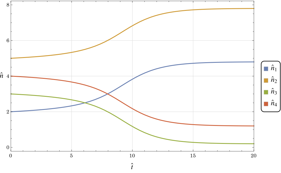
(a) number density $\hat{n}_{\alpha}$

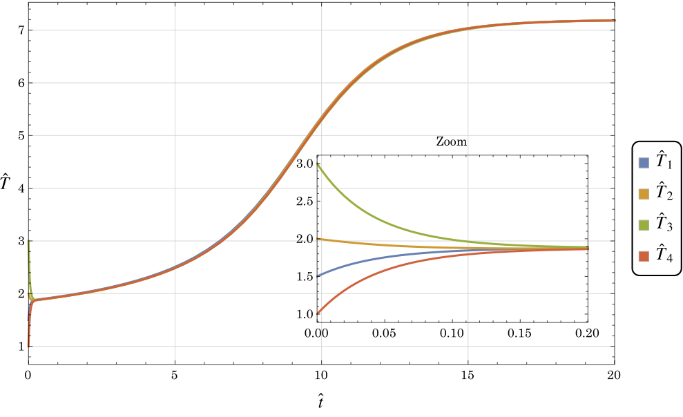
(b) Temperature $\hat{T}_{\alpha}$

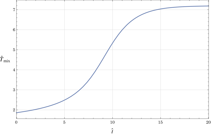
(c) Mixture temperature $\hat{T}_{mix}$

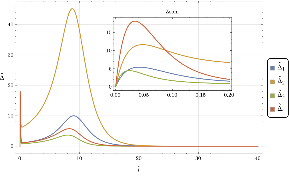
(d) The scalar moment $\hat{\Delta}_{\alpha}$

Figure 2: Relaxation to equilibrium of the different moments.

4.4.2 Case-2: Initial conditions in thermal equilibrium

We consider initial conditions that are in thermal equilibrium but not in chemical equilibrium. The initial conditions and the corresponding equilibrium states are given in Table 4. Since all the mixture components have the same temperature, the mixture is in thermal equilibrium. However, the mixture is not in chemical equilibrium since the law of mass action (71) is not satisfied. We refer to remark 7 for a distinction between a thermal and a chemical equilibrium.

Fig 3(a) shows the time variation of the different temperatures $\hat{T}_{\alpha}$. Even though we start from the same temperatures, due to a chemical non-equilibrium, the values of the different temperatures initially deviate from each other as the time progresses. Similar to the previous test case, $\hat{\Delta}_{\alpha}$ is perturbed from its initial value and we observe an initial layer which, due to a different initial data, is not as strong as the previous test case.

Initial conditions
variable	Component-1	Component-2	Component-3	Component-4
number density($\hat{n}_{\alpha}$)	2	5	3	4
Temperature($\hat{T}_{\alpha}$)	2	2	2	2
Equilibrium values
variable	Component-1	Component-2	Component-3	Component-4
number density($\hat{n}_{\alpha}$)	4.7	7.7	0.21	1.21
Temperature($\hat{T}_{\alpha}$)	7.3	7.3	7.3	7.3

Table 4: Initial conditions in thermal equilibrium and the corresponding equilibrium state.

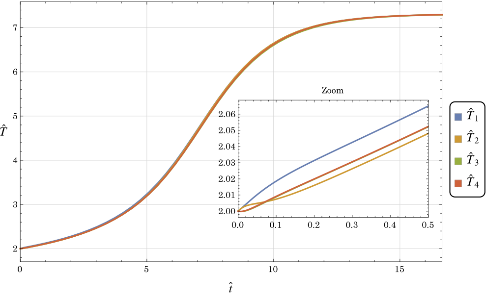
(a) Temperature $\hat{T}^{(\alpha)}$

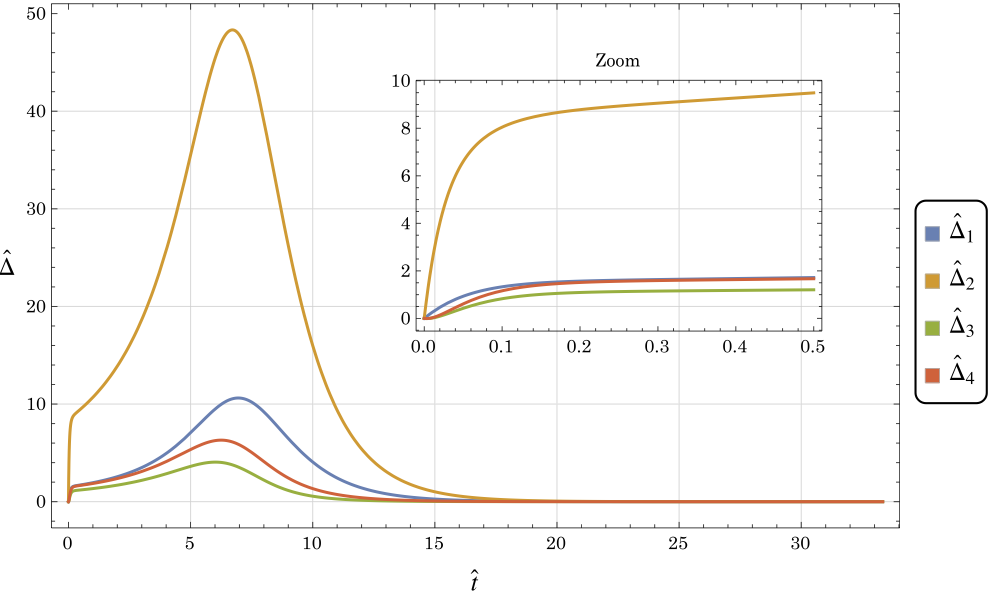
(b) The scalar moment $\hat{\Delta}^{(\alpha)}$

Figure 3: Relaxation to equilibrium of the temperature and the scalar fourteenth moment $\hat{\Delta}_{\alpha}$.

4.5 Influence of the steric factor

Table 2 shows the initial data and the corresponding equilibrium state. The activation energies and the steric factors are given in Table 3 and Table 5, respectively. Note that we only specify $s_{r}$, the value of $s_{f}$ follows from the relation in (72).

As is clear from (76), the final equilibrium state is independent of the steric factors. However, the time-scale at which the system relaxes to the equilibrium decreases as the steric factor increases—see Figure 4 that shows the variation of $\hat{T}$ for different steric factors. Following is a possible explanation for this behaviour. From (34) and (35) we conclude that increasing $s_{f}$, which also increases $s_{r}$ due to (72), the chemical collision cross-section increases, resulting in an increased number of chemical collisions. Increase in the number of collisions results in a faster relaxation of the moment system.

parameters	Forward Reaction	Reverse Reaction
$s_{f},s_{r}$	0.185	0.5
$s_{f},s_{r}$	0.22	0.6
$s_{f},s_{r}$	0.26	0.7
$s_{f},s_{r}$	0.3	0.8
$\epsilon_{f},\epsilon_{r}$	50	10

Table 5: Activation energies and the different steric factors.

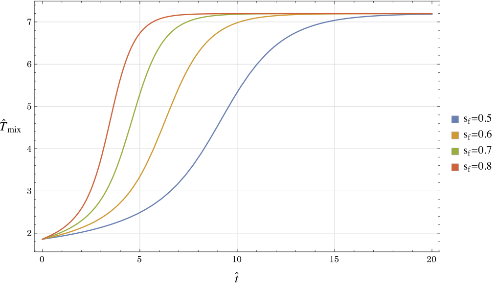
Figure 4: Mixture temperature for different steric factors.

4.6 Influence of the reaction heat ($Q$)

The initial conditions and the equilibrium states are shown in Table 2 and Table 6, respectively. Note that, unlike the steric factor, the equilibrium state changes with the heat of the reaction. We fix the steric factor to $s_{f}=0.5$.

Figure 5 shows the variation of the mixture temperature $\hat{T}$ for different values of the heat of the reaction. Since all the cases are exothermic, the equilibrium mixture temperature increases as the forward activation energy ($\epsilon_{f}$) increases. Furthermore, increasing the heat of the reaction results in a faster increase in the mixture’s temperature, leading to a faster relaxation of the moment system to the equilibrium.

Cases	$\epsilon_{f}$	$\epsilon_{r}$	$Q$	$\mathrm{T}^{(eq)}$
1	30	10	20	4.2
2	40	10	30	5.8
3	50	10	40	7.2
4	60	10	50	8.7

Table 6: Activation energies and the equilibrium values for temperatures.

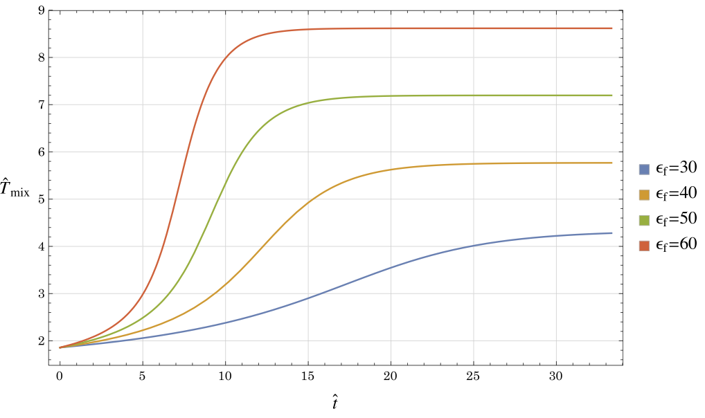
Figure 5: Mixture temperature for different reaction heats.

5 Conclusion

We derived the Grad’s–14 moment equations for a chemically reactive quaternary gaseous mixture. The main contribution was an algorithm to compute the moments of the Boltzmann’s collision operator. The algorithm relied on a novel mathematical model that describes the microscopic details of a chemically reactive collision. To develop the model, we assumed that chemical reactions affect the tangential and the normal pre-collisional relative velocity equally, leading to a symmetric collision. Using the collision model, we derived relations between the pre and the post collisional velocities. These relations helped us extend the framework for the computation of the moments of a single-gas collision operator to a reactive gas mixture. For first-order chemical kinetics, we derived reaction rates for chemical reactions outside of equilibrium and extended the Arhenius law. The reaction rates were found to have an explicit dependence on the scalar fourteenth moment, highlighting the importance of considering a fourteen moment system rather than a thirteen one. Our numerical experiments showcased that the 14-moment system can correctly reproduce the equilibrium states under different initializations and physical parameters.

6 Supplementary material: Omega Integrals

6.1 Omega integrals for the reverse reaction

$$\Omega^{(3,2)}_{\epsilon_{r}} =\frac{4m_{2}^{2}\left(2\theta_{34}m_{34}\Gamma\left(2,\frac{\epsilon_{r}}{2\theta_{34}m_{34}}\right)+Q\Gamma\left(1,\frac{\epsilon_{r}}{2\text{$\theta_{34}$}m_{34}}\right)\right)}{\text{$\theta_{34}$}M^{2}m_{12}}$$ (77)

$$\Omega^{(5,2)}_{\epsilon_{r}} =\frac{16m_{2}^{2}\left(2\theta_{34}m_{34}\Gamma\left(3,\frac{\epsilon_{r}}{2\theta_{34}m_{34}}\right)+Q\Gamma\left(2,\frac{\epsilon_{r}}{2\theta_{34}m_{34}}\right)\right)}{\theta_{34}M^{2}m_{12}}$$ (78)

$$\Omega^{(5,4)}_{\epsilon_{r}} =\frac{8m_{2}^{4}\left(Q^{2}\Gamma\left(1,\frac{\epsilon_{r}}{2\theta_{34}m_{34}}\right)+4\theta_{34}m_{34}\left(\theta_{34}m_{34}\Gamma\left(3,\frac{\epsilon_{r}}{2\theta_{34}m_{34}}\right)+Q\Gamma\left(2,\frac{\epsilon_{r}}{2\theta_{34}m_{34}}\right)\right)\right)}{\theta_{34}^{2}M^{4}m_{12}^{2}}$$ (79)

$$\Omega^{(7,2)}_{\epsilon_{r}} =\frac{64m_{2}^{2}\left(2\theta_{34}m_{34}\Gamma\left(4,\frac{\epsilon_{r}}{2\theta_{34}m_{34}}\right)+Q\Gamma\left(3,\frac{\epsilon_{r}}{2\theta_{34}m_{34}}\right)\right)}{\theta_{34}M^{2}m_{12}}$$ (80)

$$\Omega^{(9,2)}_{\epsilon_{r}} =\frac{256m_{2}^{2}\left(2\theta_{34}m_{34}\Gamma\left(5,\frac{\epsilon_{r}}{2\theta_{34}m_{34}}\right)+Q\Gamma\left(4,\frac{\epsilon_{r}}{2\theta_{34}m_{34}}\right)\right)}{\theta_{34}M^{2}m_{12}}$$ (81)

$$\Omega^{(7,4)}_{\epsilon_{r}} =\frac{32m_{2}^{4}\left(Q^{2}\Gamma\left(2,\frac{\epsilon_{r}}{2\theta_{34}m_{34}}\right)+4\theta_{34}m_{34}\left(\theta_{34}m_{34}\Gamma\left(4,\frac{\epsilon_{r}}{2\theta_{34}m_{34}}\right)+Q\Gamma\left(3,\frac{\epsilon_{r}}{2\theta_{34}m_{34}}\right)\right)\right)}{\theta_{34}^{2}M^{4}m_{12}^{2}}$$ (82)

$$\Omega^{(9,4)}_{\epsilon_{r}} =\frac{128m_{2}^{4}\left(Q^{2}\Gamma\left(3,\frac{\epsilon_{r}}{2\theta_{34}m_{34}}\right)+4\theta_{34}m_{34}\left(\theta_{34}m_{34}\Gamma\left(5,\frac{\epsilon_{r}}{2\theta_{34}m_{34}}\right)+Q\Gamma\left(4,\frac{\epsilon_{r}}{2\theta_{34}m_{34}}\right)\right)\right)}{\theta_{34}^{2}M^{4}m_{12}^{2}}$$ (83)

$$\Omega^{(11,2)}_{\epsilon_{r}} =\frac{1024m_{2}^{2}\left(2\theta_{34}m_{34}\Gamma\left(6,\frac{\epsilon_{r}}{2\theta_{34}m_{34}}\right)+Q\Gamma\left(5,\frac{\epsilon_{r}}{2\theta_{34}m_{34}}\right)\right)}{\theta_{34}M^{2}m_{12}}$$ (84)

$$\Omega^{(11,4)}_{\epsilon_{r}} =\frac{512m_{2}^{4}\left(Q^{2}\Gamma\left(4,\frac{\epsilon_{r}}{2\theta_{34}m_{34}}\right)+4\theta_{34}m_{34}\left(\theta_{34}m_{34}\Gamma\left(6,\frac{\epsilon_{r}}{2\theta_{34}m_{34}}\right)+Q\Gamma\left(5,\frac{\epsilon_{r}}{2\theta_{34}m_{34}}\right)\right)\right)}{\theta_{34}^{2}M^{4}m_{12}^{2}}$$ (85)

6.2 Omega integrals for the forward reaction

$$\Omega^{(3,2)}_{\epsilon_{f}} =\frac{4m_{4}^{2}\left(2\theta_{12}m_{12}\Gamma\left(2,\frac{\epsilon_{f}}{2\theta_{12}m_{12}}\right)-Q\Gamma\left(1,\frac{\epsilon_{f}}{2\theta_{12}m_{12}}\right)\right)}{\theta_{12}M^{2}m_{34}}$$ (86)

$$\Omega^{(5,2)}_{\epsilon_{f}} =\frac{16m_{4}^{2}\left(2\theta_{12}m_{12}\Gamma\left(3,\frac{\epsilon_{f}}{2\theta_{12}m_{12}}\right)-Q\Gamma\left(2,\frac{\epsilon_{f}}{2\theta_{12}m_{12}}\right)\right)}{\theta_{12}M^{2}m_{34}}$$ (87)

$$\Omega^{(5,4)}_{\epsilon_{f}} =\frac{8m_{4}^{4}\left(Q^{2}\Gamma\left(1,\frac{\epsilon_{f}}{2\theta_{12}m_{12}}\right)+4\theta_{12}m_{12}\left(\theta_{12}m_{12}\Gamma\left(3,\frac{\epsilon_{f}}{2\theta_{12}m_{12}}\right)-Q\Gamma\left(2,\frac{\epsilon_{f}}{2\theta_{12}m_{12}}\right)\right)\right)}{\theta_{12}^{2}M^{4}m_{34}^{2}}$$ (88)

$$\Omega^{(7,2)}_{\epsilon_{f}} =\frac{64m_{4}^{2}\left(2\theta_{12}m_{12}\Gamma\left(4,\frac{\epsilon_{f}}{2\theta_{12}m_{12}}\right)-Q\Gamma\left(3,\frac{\epsilon_{f}}{2\theta_{12}m_{12}}\right)\right)}{\theta_{12}M^{2}m_{34}}$$ (89)

$$\Omega^{(9,2)}_{\epsilon_{f}} =\frac{256m_{4}^{2}\left(2\theta_{12}m_{12}\Gamma\left(5,\frac{\epsilon_{f}}{2\theta_{12}m_{12}}\right)-Q\Gamma\left(4,\frac{\epsilon_{f}}{2\theta_{12}m_{12}}\right)\right)}{\theta_{12}M^{2}m_{34}}$$ (90)

$$\Omega^{(7,4)}_{\epsilon_{f}} =\frac{32m_{4}^{4}\left(Q^{2}\Gamma\left(2,\frac{\epsilon_{f}}{2\theta_{12}m_{12}}\right)+4\theta_{12}m_{12}\left(\theta_{12}m_{12}\Gamma\left(4,\frac{\epsilon_{f}}{2\theta_{12}m_{12}}\right)-Q\Gamma\left(3,\frac{\epsilon_{f}}{2\theta_{12}m_{12}}\right)\right)\right)}{\theta_{12}^{2}M^{4}m_{34}^{2}}$$ (91)

$$\Omega^{(9,4)}_{\epsilon_{f}} =\frac{128m_{4}^{4}\left(Q^{2}\Gamma\left(3,\frac{\epsilon_{f}}{2\theta_{12}m_{12}}\right)+4\theta_{12}m_{12}\left(\theta_{12}m_{12}\Gamma\left(5,\frac{\epsilon_{f}}{2\theta_{12}m_{12}}\right)-Q\Gamma\left(4,\frac{\epsilon_{f}}{2\theta_{12}m_{12}}\right)\right)\right)}{\theta_{12}^{2}M^{4}m_{34}^{2}}$$ (92)

$$\Omega^{(11,2)}_{\epsilon_{f}} =\frac{1024m_{4}^{2}\left(2\theta_{12}m_{12}\Gamma\left(6,\frac{\epsilon_{f}}{2\theta_{12}m_{12}}\right)-Q\Gamma\left(5,\frac{\epsilon_{f}}{2\theta_{12}m_{12}}\right)\right)}{\theta_{12}M^{2}m_{34}}$$ (93)

$$\Omega^{(11,4)}_{\epsilon_{f}} =\frac{512m_{4}^{4}\left(Q^{2}\Gamma\left(4,\frac{\epsilon_{f}}{2\theta_{12}m_{12}}\right)+4\theta_{12}m_{12}\left(\theta_{12}m_{12}\Gamma\left(6,\frac{\epsilon_{f}}{2\theta_{12}m_{12}}\right)-Q\Gamma\left(5,\frac{\epsilon_{f}}{2\theta_{12}m_{12}}\right)\right)\right)}{\theta_{12}^{2}M^{4}m_{34}^{2}}$$ (94)

where $M=m_{1}+m_{2}=m_{3}+m_{4}$.

7 Supplementary material: Chemical production terms

7.1 Mass Balance

• Mass Balance

  $$\mathcal{P}^{\alpha=1}_{R,0}=d_{r}^{2}\tilde{n}_{34}\mu_{12}\exp\left[{-\frac{\epsilon_{r}}{2\theta_{34}m_{34}}}\right]-d_{f}^{2}\tilde{n}_{12}\mu_{12}\exp\left[{-\frac{\epsilon_{f}}{2\theta_{12}m_{12}}}\right]+\Delta^{r(1)0}$$ (95)

  $$\mathcal{P}^{\alpha=2}_{R,0}=d_{r}^{2}\tilde{n}_{34}\mu_{21}\exp\left[{-\frac{\epsilon_{r}}{2\theta_{34}m_{34}}}\right]-d_{f}^{2}\tilde{n}_{12}\mu_{21}\exp\left[{-\frac{\epsilon_{f}}{2\theta_{12}m_{12}}}\right]+\Delta^{r(2)0}$$ (96)

  $$\mathcal{P}^{\alpha=3}_{R,0}=d_{f}^{2}\tilde{n}_{12}\mu_{34}\exp\left[{-\frac{\epsilon_{f}}{2\theta_{12}m_{12}}}\right]-d_{r}^{2}\tilde{n}_{34}\mu_{34}\exp\left[{-\frac{\epsilon_{r}}{2\theta_{34}m_{34}}}\right]+\Delta^{r(3)0}$$ (97)

  $$\mathcal{P}^{\alpha=4}_{R,0}=d_{f}^{2}\tilde{n}_{12}\mu_{43}\exp\left[{-\frac{\epsilon_{f}}{2\theta_{12}m_{12}}}\right]-d_{r}^{2}\tilde{n}_{34}\mu_{43}\exp\left[{-\frac{\epsilon_{r}}{2\theta_{34}m_{34}}}\right]+\Delta^{r(4)0}$$ (98)

where $\tilde{n}_{34}=4\sqrt{\pi}\sqrt{\theta_{34}}Mn_{3}n_{4}$, $\tilde{n}_{12}=4\sqrt{\pi}\sqrt{\theta_{12}}Mn_{1}n_{2}$ and $\Delta^{r(\alpha)0}$ is the contribution from $\Delta_{\alpha}$. Explicit expressions for $\Delta^{r(\alpha)0}$ have been given in subsection 8.2 and subsection 8.1.

7.2 Momentum Balance

The generic form of the momentum production can be given as

$$\mathcal{P}^{\alpha}_{R,i}=\sum_{\gamma=1}^{4}\left(\tau^{\alpha}_{\gamma}u^{(\gamma)}_{i}+\omega^{\alpha}_{\gamma}q^{(\gamma)}_{i}\right)$$ (99)

The coefficients $\tau^{\alpha}_{\gamma}$ and $\omega^{\alpha}_{\gamma}$ can now be given as

7.2.1 Component-1

$$\tau^{(1)}_{1}=\frac{1}{6}\beta_{f}\sqrt{\theta_{1}}\mu_{12}\left(\theta_{12}^{2}m_{12}^{2}\left(24\theta_{1}^{2}+8\theta_{1}(5\theta_{2}-7\theta_{12})+3\theta_{2}(5\theta_{2}-14\theta_{12})\right)+2\theta_{1}\theta_{12}m_{12}\epsilon_{f}(4\theta_{1}-7\theta_{12}+5\theta_{2})+\theta_{1}^{2}\epsilon_{f}^{2}\right)\\ \\$$

$$\tau^{(1)}_{2}=-\frac{1}{6}\beta_{f}\theta_{1}\sqrt{\theta_{2}}\mu_{12}\left(\theta_{2}\left(4\theta_{12}^{2}m_{12}^{2}+3\theta_{12}m_{12}\epsilon_{f}+\epsilon_{f}^{2}\right)+\theta_{12}m_{12}(5\theta_{1}-14\theta_{12})(\theta_{12}m_{12}+\epsilon_{f})\right)\\ \\$$

$$\tau^{(1)}_{3}=\frac{1}{6}\beta_{r}\sqrt{\theta_{3}}\mu_{12}\left(\theta_{34}^{2}m_{34}^{2}\left(-24\theta_{3}^{2}+4\mu_{34}(2\theta_{34})(6\theta_{3}-14\theta_{34}+5\theta_{4})+56\theta_{3}\theta_{34}-40\theta_{3}\theta_{4}+42\theta_{34}\theta_{4}-15\theta_{4}^{2}\right)+\theta_{34}m_{34}\epsilon_{r}(\mu_{34}(2\theta_{34})(8\theta_{3}-14\theta_{34}+5\theta_{4})-2\theta_{3}(4\theta_{3}-7\theta_{34}+5\theta_{4}))+\theta_{3}\epsilon_{r}^{2}(\theta_{3}(\mu_{34}-1)+\theta_{4}\mu_{34})\right)\\ \\$$

$$\tau^{(1)}_{4}=-\frac{1}{6}\beta_{r}\sqrt{\theta_{4}}\mu_{12}\left(\mu_{34}(2\theta_{34})\left(\theta_{4}\left(24\theta_{34}^{2}m_{34}^{2}+8\theta_{34}m_{34}\epsilon_{r}+\epsilon_{r}^{2}\right)+\theta_{34}m_{34}(5\theta_{3}-14\theta_{34})(4\theta_{34}m_{34}+\epsilon_{r})\right)-\theta_{3}\theta_{4}\left(4\theta_{34}^{2}m_{34}^{2}+3\theta_{34}m_{34}\epsilon_{r}+\epsilon_{r}^{2}\right)+\theta_{3}\theta_{34}(-m_{34})(5\theta_{3}-14\theta_{34})(\theta_{34}m_{34}+\epsilon_{r})\right)\\ \\$$

$$\omega^{(1)}_{1}=-\frac{1}{15}\beta_{f}\sqrt{\theta_{1}}\mu_{12}\left(\theta_{12}^{2}m_{12}^{2}\left(24\theta_{1}^{2}+40\theta_{1}(\theta_{2}-\theta_{12})+15\theta_{2}(\theta_{2}-2\theta_{12})\right)+2\theta_{1}\theta_{12}m_{12}\epsilon_{f}(4\theta_{1}-5\theta_{12}+5\theta_{2})+\theta_{1}^{2}\epsilon_{f}^{2}\right)\\ \\$$

$$\omega^{(1)}_{2}=\frac{1}{15}\beta_{f}\theta_{1}\sqrt{\theta_{2}}\mu_{12}\left(\theta_{2}\left(4\theta_{12}^{2}m_{12}^{2}+3\theta_{12}m_{12}\epsilon_{f}+\epsilon_{f}^{2}\right)+5\theta_{12}m_{12}(\theta_{1}-2\theta_{12})(\theta_{12}m_{12}+\epsilon_{f})\right)\\ \\$$

$$\omega^{(1)}_{3}=-\frac{1}{15}\beta_{r}\sqrt{\theta_{3}}\mu_{12}\left(\theta_{34}^{2}m_{34}^{2}\left(-24\theta_{3}^{2}+4\mu_{34}(2\theta_{34})(6\theta_{3}+5(\theta_{4}-2\theta_{34}))+40\theta_{3}\theta_{34}-40\theta_{3}\theta_{4}+30\theta_{34}\theta_{4}-15\theta_{4}^{2}\right)+\theta_{34}m_{34}\epsilon_{r}(\mu_{34}(2\theta_{34})(8\theta_{3}+5(\theta_{4}-2\theta_{34}))-2\theta_{3}(4\theta_{3}-5\theta_{34}+5\theta_{4}))+\theta_{3}\epsilon_{r}^{2}(\theta_{3}(\mu_{34}-1)+\theta_{4}\mu_{34})\right)\\ \\$$

$$\omega^{(1)}_{4}=\frac{1}{15}\beta_{r}\sqrt{\theta_{4}}\mu_{12}\left(\mu_{34}(2\theta_{34})\left(\theta_{4}\left(24\theta_{34}^{2}m_{34}^{2}+8\theta_{34}m_{34}\epsilon_{r}+\epsilon_{r}^{2}\right)+5\theta_{34}m_{34}(\theta_{3}-2\theta_{34})(4\theta_{34}m_{34}+\epsilon_{r})\right)-\theta_{3}\theta_{4}\left(4\theta_{34}^{2}m_{34}^{2}+3\theta_{34}m_{34}\epsilon_{r}+\epsilon_{r}^{2}\right)-5\theta_{3}\theta_{34}m_{34}(\theta_{3}-2\theta_{34})(\theta_{34}m_{34}+\epsilon_{r})\right)\\ \\$$

7.2.2 Component-2

$$\tau^{(2)}_{1}=-\frac{1}{6}\beta_{f}\sqrt{\theta_{1}}\theta_{2}\mu_{21}\left(\theta_{12}^{2}m_{12}^{2}(4\theta_{1}-14\theta_{12}+5\theta_{2})+\theta_{12}m_{12}\epsilon_{f}(3\theta_{1}-14\theta_{12}+5\theta_{2})+\theta_{1}\epsilon_{f}^{2}\right)\\ \\$$

$$\tau^{(2)}_{2}=\frac{1}{6}\beta_{f}\sqrt{\theta_{2}}\mu_{21}\left(3\theta_{1}\theta_{12}^{2}m_{12}^{2}(5\theta_{1}-14\theta_{12})+\theta_{2}^{2}\left(24\theta_{12}^{2}m_{12}^{2}+8\theta_{12}m_{12}\epsilon_{f}+\epsilon_{f}^{2}\right)+2\theta_{12}\theta_{2}m_{12}(5\theta_{1}-7\theta_{12})(4\theta_{12}m_{12}+\epsilon_{f})\right)\\ \\$$

$$\tau^{(2)}_{3}=-\frac{1}{6}\beta_{r}\sqrt{\theta_{3}}\mu_{21}\left(\theta_{34}^{2}m_{34}^{2}(4\mu_{34}(2\theta_{34})(6\theta_{3}-14\theta_{34}+5\theta_{4})+\theta_{4}(-4\theta_{3}+14\theta_{34}-5\theta_{4}))+\theta_{34}m_{34}\epsilon_{r}(\mu_{34}(2\theta_{34})(8\theta_{3}-14\theta_{34}+5\theta_{4})+\theta_{4}(-3\theta_{3}+14\theta_{34}-5\theta_{4}))+\theta_{3}\epsilon_{r}^{2}(\theta_{3}\mu_{34}+\theta_{4}(\mu_{34}-1))\right)\\ \\$$

$$\tau^{(2)}_{4}=\frac{1}{6}\beta_{r}\sqrt{\theta_{4}}\mu_{21}\left(\theta_{34}^{2}m_{34}^{2}\left(-15\theta_{3}^{2}+4\mu_{34}(2\theta_{34})(5\theta_{3}-14\theta_{34}+6\theta_{4})+42\theta_{3}\theta_{34}-40\theta_{3}\theta_{4}+56\theta_{34}\theta_{4}-24\theta_{4}^{2}\right)+\theta_{34}m_{34}\epsilon_{r}(\mu_{34}(2\theta_{34})(5\theta_{3}-14\theta_{34}+8\theta_{4})-2\theta_{4}(5\theta_{3}-7\theta_{34}+4\theta_{4}))+\theta_{4}\epsilon_{r}^{2}(\theta_{3}\mu_{34}+\theta_{4}(\mu_{34}-1))\right)\\ \\$$

$$\omega^{(2)}_{1}=\frac{1}{15}\beta_{f}\sqrt{\theta_{1}}\theta_{2}\mu_{21}\left(\theta_{12}^{2}m_{12}^{2}(4\theta_{1}+5(\theta_{2}-2\theta_{12}))+\theta_{12}m_{12}\epsilon_{f}(3\theta_{1}+5(\theta_{2}-2\theta_{12}))+\theta_{1}\epsilon_{f}^{2}\right)\\ \\$$

$$\omega^{(2)}_{2}=-\frac{1}{15}\beta_{f}\sqrt{\theta_{2}}\mu_{21}\left(15\theta_{1}\theta_{12}^{2}m_{12}^{2}(\theta_{1}-2\theta_{12})+\theta_{2}^{2}\left(24\theta_{12}^{2}m_{12}^{2}+8\theta_{12}m_{12}\epsilon_{f}+\epsilon_{f}^{2}\right)+10\theta_{12}\theta_{2}m_{12}(\theta_{1}-\theta_{12})(4\theta_{12}m_{12}+\epsilon_{f})\right)\\ \\$$

$$\omega^{(2)}_{3}=\frac{1}{15}\beta_{r}\sqrt{\theta_{3}}\mu_{21}\left(\theta_{34}^{2}m_{34}^{2}(4\mu_{34}(2\theta_{34})(6\theta_{3}+5(\theta_{4}-2\theta_{34}))+\theta_{4}(-4\theta_{3}+10\theta_{34}-5\theta_{4}))+\theta_{34}m_{34}\epsilon_{r}(\mu_{34}(2\theta_{34})(8\theta_{3}+5(\theta_{4}-2\theta_{34}))+\theta_{4}(-3\theta_{3}+10\theta_{34}-5\theta_{4}))+\theta_{3}\epsilon_{r}^{2}(\theta_{3}\mu_{34}+\theta_{4}(\mu_{34}-1))\right)\\ \\$$

$$\omega^{(2)}_{4}=-\frac{1}{15}\beta_{r}\sqrt{\theta_{4}}\mu_{21}\left(\theta_{34}^{2}m_{34}^{2}\left(-15\theta_{3}^{2}+4\mu_{34}(2\theta_{34})(5\theta_{3}-10\theta_{34}+6\theta_{4})+30\theta_{3}\theta_{34}-40\theta_{3}\theta_{4}+40\theta_{34}\theta_{4}-24\theta_{4}^{2}\right)+\theta_{34}m_{34}\epsilon_{r}(\mu_{34}(2\theta_{34})(5\theta_{3}-10\theta_{34}+8\theta_{4})-2\theta_{4}(5\theta_{3}-5\theta_{34}+4\theta_{4}))+\theta_{4}\epsilon_{r}^{2}(\theta_{3}\mu_{34}+\theta_{4}(\mu_{34}-1))\right)\\ \\$$

7.2.3 Component-3

$$\tau^{(3)}_{1}=\frac{1}{6}\beta_{f}\sqrt{\theta_{1}}\mu_{34}\left(\theta_{12}^{2}m_{12}^{2}\left(-24\theta_{1}^{2}+4\mu_{21}(2\theta_{12})(6\theta_{1}-14\theta_{12}+5\theta_{2})+56\theta_{1}\theta_{12}-40\theta_{1}\theta_{2}+42\theta_{12}\theta_{2}-15\theta_{2}^{2}\right)+\theta_{12}m_{12}\epsilon_{f}(\mu_{21}(2\theta_{12})(8\theta_{1}-14\theta_{12}+5\theta_{2})-2\theta_{1}(4\theta_{1}-7\theta_{12}+5\theta_{2}))+\theta_{1}\epsilon_{f}^{2}(\theta_{1}(\mu_{21}-1)+\theta_{2}\mu_{21})\right)\\ \\$$

$$\tau^{(3)}_{2}=-\frac{1}{6}\beta_{f}\sqrt{\theta_{2}}\mu_{34}\left(\mu_{21}(2\theta_{12})\left(\theta_{2}\left(24\theta_{12}^{2}m_{12}^{2}+8\theta_{12}m_{12}\epsilon_{f}+\epsilon_{f}^{2}\right)+\theta_{12}m_{12}(5\theta_{1}-14\theta_{12})(4\theta_{12}m_{12}+\epsilon_{f})\right)-\theta_{1}\theta_{2}\left(4\theta_{12}^{2}m_{12}^{2}+3\theta_{12}m_{12}\epsilon_{f}+\epsilon_{f}^{2}\right)+\theta_{1}\theta_{12}(-m_{12})(5\theta_{1}-14\theta_{12})(\theta_{12}m_{12}+\epsilon_{f})\right)\\ \\$$

$$\tau^{(3)}_{3}=\frac{1}{6}\beta_{r}\sqrt{\theta_{3}}\mu_{34}\left(\theta_{34}^{2}m_{34}^{2}\left(24\theta_{3}^{2}+8\theta_{3}(5\theta_{4}-7\theta_{34})+3\theta_{4}(5\theta_{4}-14\theta_{34})\right)+2\theta_{3}\theta_{34}m_{34}\epsilon_{r}(4\theta_{3}-7\theta_{34}+5\theta_{4})+\theta_{3}^{2}\epsilon_{r}^{2}\right)\\ \\$$

$$\tau^{(3)}_{4}=-\frac{1}{6}\beta_{r}\theta_{3}\sqrt{\theta_{4}}\mu_{34}\left(\theta_{4}\left(4\theta_{34}^{2}m_{34}^{2}+3\theta_{34}m_{34}\epsilon_{r}+\epsilon_{r}^{2}\right)+\theta_{34}m_{34}(5\theta_{3}-14\theta_{34})(\theta_{34}m_{34}+\epsilon_{r})\right)\\ \\$$

$$\omega^{(3)}_{1}=-\frac{1}{15}\beta_{f}\sqrt{\theta_{1}}\mu_{34}\left(\theta_{12}^{2}m_{12}^{2}\left(-24\theta_{1}^{2}+4\mu_{21}(2\theta_{12})(6\theta_{1}+5(\theta_{2}-2\theta_{12}))+40\theta_{1}\theta_{12}-40\theta_{1}\theta_{2}+30\theta_{12}\theta_{2}-15\theta_{2}^{2}\right)+\theta_{12}m_{12}\epsilon_{f}(\mu_{21}(2\theta_{12})(8\theta_{1}+5(\theta_{2}-2\theta_{12}))-2\theta_{1}(4\theta_{1}-5\theta_{12}+5\theta_{2}))+\theta_{1}\epsilon_{f}^{2}(\theta_{1}(\mu_{21}-1)+\theta_{2}\mu_{21})\right)\\ \\$$

$$\omega^{(3)}_{2}=\frac{1}{15}\beta_{f}\sqrt{\theta_{2}}\mu_{34}\left(\mu_{21}(2\theta_{12})\left(\theta_{2}\left(24\theta_{12}^{2}m_{12}^{2}+8\theta_{12}m_{12}\epsilon_{f}+\epsilon_{f}^{2}\right)+5\theta_{12}m_{12}(\theta_{1}-2\theta_{12})(4\theta_{12}m_{12}+\epsilon_{f})\right)-\theta_{1}\theta_{2}\left(4\theta_{12}^{2}m_{12}^{2}+3\theta_{12}m_{12}\epsilon_{f}+\epsilon_{f}^{2}\right)-5\theta_{1}\theta_{12}m_{12}(\theta_{1}-2\theta_{12})(\theta_{12}m_{12}+\epsilon_{f})\right)\\ \\$$

$$\omega^{(3)}_{3}=-\frac{1}{15}\beta_{r}\sqrt{\theta_{3}}\mu_{34}\left(\theta_{34}^{2}m_{34}^{2}\left(24\theta_{3}^{2}+40\theta_{3}(\theta_{4}-\theta_{34})+15\theta_{4}(\theta_{4}-2\theta_{34})\right)+2\theta_{3}\theta_{34}m_{34}\epsilon_{r}(4\theta_{3}-5\theta_{34}+5\theta_{4})+\theta_{3}^{2}\epsilon_{r}^{2}\right)\\ \\$$

$$\omega^{(3)}_{4}=\frac{1}{15}\beta_{r}\theta_{3}\sqrt{\theta_{4}}\mu_{34}\left(\theta_{4}\left(4\theta_{34}^{2}m_{34}^{2}+3\theta_{34}m_{34}\epsilon_{r}+\epsilon_{r}^{2}\right)+5\theta_{34}m_{34}(\theta_{3}-2\theta_{34})(\theta_{34}m_{34}+\epsilon_{r})\right)\\ \\$$

7.2.4 Component-4

$$\tau^{(4)}_{1}=-\frac{1}{6}\beta_{f}\sqrt{\theta_{1}}\mu_{43}\left(\theta_{12}^{2}m_{12}^{2}(4\mu_{12}(2\theta_{12})(6\theta_{1}-14\theta_{12}+5\theta_{2})+\theta_{2}(-4\theta_{1}+14\theta_{12}-5\theta_{2}))+\theta_{12}m_{12}\epsilon_{f}(\mu_{12}(2\theta_{12})(8\theta_{1}-14\theta_{12}+5\theta_{2})+\theta_{2}(-3\theta_{1}+14\theta_{12}-5\theta_{2}))+\theta_{1}\epsilon_{f}^{2}(\theta_{1}\mu_{12}+\theta_{2}(\mu_{12}-1))\right)\\ \\$$

$$\tau^{(4)}_{2}=\frac{1}{6}\beta_{f}\sqrt{\theta_{2}}\mu_{43}\left(\theta_{12}^{2}m_{12}^{2}\left(-15\theta_{1}^{2}+4\mu_{12}(2\theta_{12})(5\theta_{1}-14\theta_{12}+6\theta_{2})+42\theta_{1}\theta_{12}-40\theta_{1}\theta_{2}+56\theta_{12}\theta_{2}-24\theta_{2}^{2}\right)+\theta_{12}m_{12}\epsilon_{f}(\mu_{12}(2\theta_{12})(5\theta_{1}-14\theta_{12}+8\theta_{2})-2\theta_{2}(5\theta_{1}-7\theta_{12}+4\theta_{2}))+\theta_{2}\epsilon_{f}^{2}(\theta_{1}\mu_{12}+\theta_{2}(\mu_{12}-1))\right)\\ \\$$

$$\tau^{(4)}_{3}=-\frac{1}{6}\beta_{r}\sqrt{\theta_{3}}\theta_{4}\mu_{43}\left(\theta_{34}^{2}m_{34}^{2}(4\theta_{3}-14\theta_{34}+5\theta_{4})+\theta_{34}m_{34}\epsilon_{r}(3\theta_{3}-14\theta_{34}+5\theta_{4})+\theta_{3}\epsilon_{r}^{2}\right)\\ \\$$

$$\tau^{(4)}_{4}=\frac{1}{6}\beta_{r}\sqrt{\theta_{4}}\mu_{43}\left(3\theta_{3}\theta_{34}^{2}m_{34}^{2}(5\theta_{3}-14\theta_{34})+\theta_{4}^{2}\left(24\theta_{34}^{2}m_{34}^{2}+8\theta_{34}m_{34}\epsilon_{r}+\epsilon_{r}^{2}\right)+2\theta_{34}\theta_{4}m_{34}(5\theta_{3}-7\theta_{34})(4\theta_{34}m_{34}+\epsilon_{r})\right)\\ \\$$

$$\omega^{(4)}_{1}=\frac{1}{15}\beta_{f}\sqrt{\theta_{1}}\mu_{43}\left(\theta_{12}^{2}m_{12}^{2}(4\mu_{12}(2\theta_{12})(6\theta_{1}+5(\theta_{2}-2\theta_{12}))+\theta_{2}(-4\theta_{1}+10\theta_{12}-5\theta_{2}))+\theta_{12}m_{12}\epsilon_{f}(\mu_{12}(2\theta_{12})(8\theta_{1}+5(\theta_{2}-2\theta_{12}))+\theta_{2}(-3\theta_{1}+10\theta_{12}-5\theta_{2}))+\theta_{1}\epsilon_{f}^{2}(\theta_{1}\mu_{12}+\theta_{2}(\mu_{12}-1))\right)\\ \\$$

$$\omega^{(4)}_{2}=-\frac{1}{15}\beta_{f}\sqrt{\theta_{2}}\mu_{43}\left(\theta_{12}^{2}m_{12}^{2}\left(-15\theta_{1}^{2}+4\mu_{12}(2\theta_{12})(5\theta_{1}-10\theta_{12}+6\theta_{2})+30\theta_{1}\theta_{12}-40\theta_{1}\theta_{2}+40\theta_{12}\theta_{2}-24\theta_{2}^{2}\right)+\theta_{12}m_{12}\epsilon_{f}(\mu_{12}(2\theta_{12})(5\theta_{1}-10\theta_{12}+8\theta_{2})-2\theta_{2}(5\theta_{1}-5\theta_{12}+4\theta_{2}))+\theta_{2}\epsilon_{f}^{2}(\theta_{1}\mu_{12}+\theta_{2}(\mu_{12}-1))\right)\\ \\$$

$$\omega^{(4)}_{3}=\frac{1}{15}\beta_{r}\sqrt{\theta_{3}}\theta_{4}\mu_{43}\left(\theta_{34}^{2}m_{34}^{2}(4\theta_{3}+5(\theta_{4}-2\theta_{34}))+\theta_{34}m_{34}\epsilon_{r}(3\theta_{3}+5(\theta_{4}-2\theta_{34}))+\theta_{3}\epsilon_{r}^{2}\right)\\ \\$$

$$\omega^{(4)}_{4}=-\frac{1}{15}\beta_{r}\sqrt{\theta_{4}}\mu_{43}\left(15\theta_{3}\theta_{34}^{2}m_{34}^{2}(\theta_{3}-2\theta_{34})+\theta_{4}^{2}\left(24\theta_{34}^{2}m_{34}^{2}+8\theta_{34}m_{34}\epsilon_{r}+\epsilon_{r}^{2}\right)+10\theta_{34}\theta_{4}m_{34}(\theta_{3}-\theta_{34})(4\theta_{34}m_{34}+\epsilon_{r})\right)\\ \\$$

$$\beta_{f}=\left(\frac{\sqrt{\pi}d_{12}^{2}Mn_{1}n_{2}s_{f}^{2}}{\theta_{12}^{7/2}m_{12}^{2}}\right)\exp\left[{-\frac{\epsilon_{f}}{2\theta_{12}m_{12}}}\right],\quad\beta_{r}=\left(\frac{\sqrt{\pi}d_{34}^{2}Mn_{3}n_{4}s_{r}^{2}}{\theta_{34}^{7/2}m_{34}^{2}}\right)\exp\left[{-\frac{\epsilon_{r}}{2\theta_{34}m_{34}}}\right]$$ (100)

7.3 Energy Balance

The following are the production terms corresponding to energy balance for all the components present in the mixture.

7.3.1 Component-1

$$\mathcal{P}^{\alpha}_{R,1}=\frac{1}{8}\beta_{r}\theta_{34}^{2}\mu_{12}\left(\theta_{34}(2\theta_{34})e^{\frac{\epsilon_{r}}{2\theta_{34}m_{34}}}(\theta_{34}m_{34}\Omega^{(5,2)}_{\epsilon_{r}}-2\epsilon_{r}\Omega^{(3,2)}_{\epsilon_{r}})+8\left(2\theta_{34}\mu_{34}^{2}(2\theta_{34})(4\theta_{34}m_{34}+\epsilon_{r})-2\theta_{3}\mu_{34}(2\theta_{34})(4\theta_{34}m_{34}+\epsilon_{r})+\theta_{3}(\theta_{34}m_{34}(4\theta_{3}+3\theta_{4})+\theta_{3}\epsilon_{r})\right)\right)-\beta_{f}\theta_{1}\theta_{12}^{2}\mu_{12}(\theta_{12}m_{12}(4\theta_{1}+3\theta_{2})+\theta_{1}\epsilon_{f})+\Delta^{r(1)1}\\ \\$$

7.3.2 Component-2

$$\mathcal{P}^{\alpha}_{R,1}=\frac{\beta_{r}\theta_{34}^{2}}{8\mu_{21}}\left(\theta_{34}\mu_{12}^{2}(2\theta_{34})e^{\frac{\epsilon_{r}}{2\theta_{34}m_{34}}}(\theta_{34}m_{34}\Omega^{(5,2)}_{\epsilon_{r}}-2\epsilon_{r}\Omega^{(3,2)}_{\epsilon_{r}})+8\mu_{21}^{2}\left(2\theta_{34}\mu_{34}^{2}(2\theta_{34})(4\theta_{34}m_{34}+\epsilon_{r})-2\theta_{4}\mu_{34}(2\theta_{34})(4\theta_{34}m_{34}+\epsilon_{r})+\theta_{4}(\theta_{34}m_{34}(3\theta_{3}+4\theta_{4})+\theta_{4}\epsilon_{r})\right)\right)-\beta_{f}\theta_{12}^{2}\theta_{2}\mu_{21}(\theta_{12}m_{12}(3\theta_{1}+4\theta_{2})+\theta_{2}\epsilon_{f})+\Delta^{r(2)1}\\ \\$$

7.3.3 Component-3

$$\mathcal{P}^{\alpha}_{R,1}=\frac{1}{8}\beta_{f}\theta_{12}^{2}\mu_{34}\left(\theta_{12}(2\theta_{12})e^{\frac{\epsilon_{f}}{2\theta_{12}m_{12}}}(\theta_{12}m_{12}\Omega^{(5,2)}_{\epsilon_{f}}-2\epsilon_{f}\Omega^{(3,2)}_{\epsilon_{f}})+8\left(2\theta_{12}\mu_{21}^{2}(2\theta_{12})(4\theta_{12}m_{12}+\epsilon_{f})-2\theta_{1}\mu_{21}(2\theta_{12})(4\theta_{12}m_{12}+\epsilon_{f})+\theta_{1}(\theta_{12}m_{12}(4\theta_{1}+3\theta_{2})+\theta_{1}\epsilon_{f})\right)\right)-\beta_{r}\theta_{3}\theta_{34}^{2}\mu_{34}(\theta_{34}m_{34}(4\theta_{3}+3\theta_{4})+\theta_{3}\epsilon_{r})+\Delta^{r(3)1}\\ \\$$

7.3.4 Component-4

$$\mathcal{P}^{\alpha}_{R,1}=\frac{\beta_{f}\theta_{12}^{2}}{8\mu_{43}}\left(\theta_{12}\mu_{34}^{2}(2\theta_{12})e^{\frac{\epsilon_{f}}{2\theta_{12}m_{12}}}(\theta_{12}m_{12}\Omega^{(5,2)}_{\epsilon_{f}}-2\epsilon_{f}\Omega^{(3,2)}_{\epsilon_{f}})+8\mu_{43}^{2}\left(2\theta_{12}\mu_{12}^{2}(2\theta_{12})(4\theta_{12}m_{12}+\epsilon_{f})-2\theta_{2}\mu_{12}(2\theta_{12})(4\theta_{12}m_{12}+\epsilon_{f})+\theta_{2}(\theta_{12}m_{12}(3\theta_{1}+4\theta_{2})+\theta_{2}\epsilon_{f})\right)\right)-\beta_{r}\theta_{34}^{2}\theta_{4}\mu_{43}(\theta_{34}m_{34}(3\theta_{3}+4\theta_{4})+\theta_{4}\epsilon_{r})+\Delta^{r(4)1}\\ \\$$

7.4 Stress Production

The production term for the stress tensor can be given in a generic form as

$$\mathcal{P}^{\alpha}_{R,ij}=\sum_{\gamma=1}^{4}\left(\xi^{(\alpha)}_{\gamma}\sigma^{(\alpha)}_{ij}\right)$$ (101)

The coefficients $\xi^{(\alpha)}_{\gamma}$ can now be given as

7.4.1 Component-1

$$\xi^{(1)}_{1}=-\frac{1}{15}\beta_{f}\theta_{1}\mu_{12}\left(\theta_{12}^{2}m_{12}^{2}\left(24\theta_{1}^{2}+40\theta_{1}\theta_{2}+15\theta_{2}^{2}\right)+2\theta_{1}\theta_{12}m_{12}\epsilon_{f}(4\theta_{1}+5\theta_{2})+\theta_{1}^{2}\epsilon_{f}^{2}\right)$$

$$\xi^{(1)}_{2}=\frac{1}{15}\beta_{f}\theta_{1}^{2}\theta_{2}\mu_{12}\left(\theta_{12}^{2}m_{12}^{2}+2\theta_{12}m_{12}\epsilon_{f}-\epsilon_{f}^{2}\right)$$

$$\xi^{(1)}_{3}=\frac{1}{15}\beta_{r}\theta_{3}\mu_{12}\left(\theta_{34}^{2}m_{34}^{2}\left(24\theta_{3}^{2}+48\theta_{34}\mu_{34}^{2}(2\theta_{34})-8\mu_{34}(2\theta_{34})(6\theta_{3}+5\theta_{4})+40\theta_{3}\theta_{4}+15\theta_{4}^{2}\right)+2\theta_{34}m_{34}\epsilon_{r}\left(8\theta_{34}\mu_{34}^{2}(2\theta_{34})-\mu_{34}(2\theta_{34})(8\theta_{3}+5\theta_{4})+\theta_{3}(4\theta_{3}+5\theta_{4})\right)+\epsilon_{r}^{2}\left(\theta_{3}^{2}+2\theta_{34}\mu_{34}^{2}(2\theta_{34})-2\theta_{3}\mu_{34}(2\theta_{34})\right)\right)\\ \\$$

$$\xi^{(1)}_{4}=\frac{1}{15}\beta_{r}\theta_{4}\mu_{12}\left(\theta_{3}^{2}\left(-\theta_{34}^{2}m_{34}^{2}-2\theta_{34}m_{34}\epsilon_{r}+\epsilon_{r}^{2}\right)+2\theta_{34}\mu_{34}^{2}(2\theta_{34})\left(24\theta_{34}^{2}m_{34}^{2}+8\theta_{34}m_{34}\epsilon_{r}+\epsilon_{r}^{2}\right)-2\theta_{3}\mu_{34}(2\theta_{34})\left(4\theta_{34}^{2}m_{34}^{2}+3\theta_{34}m_{34}\epsilon_{r}+\epsilon_{r}^{2}\right)\right)\\ \\$$

7.4.2 Component-2

$$\xi^{(2)}_{1}=\frac{1}{15}\beta_{f}\theta_{1}\theta_{2}^{2}\mu_{21}\left(\theta_{12}^{2}m_{12}^{2}+2\theta_{12}m_{12}\epsilon_{f}-\epsilon_{f}^{2}\right)\\ \\$$

$$\xi^{(2)}_{2}=-\frac{1}{15}\beta_{f}\theta_{2}\mu_{21}\left(\theta_{12}^{2}m_{12}^{2}\left(15\theta_{1}^{2}+40\theta_{1}\theta_{2}+24\theta_{2}^{2}\right)+2\theta_{12}\theta_{2}m_{12}\epsilon_{f}(5\theta_{1}+4\theta_{2})+\theta_{2}^{2}\epsilon_{f}^{2}\right)\\ \\$$

$$\xi^{(2)}_{3}=\frac{1}{15}\beta_{r}\theta_{3}\mu_{21}\left(2\theta_{34}\mu_{34}^{2}(2\theta_{34})\left(24\theta_{34}^{2}m_{34}^{2}+8\theta_{34}m_{34}\epsilon_{r}+\epsilon_{r}^{2}\right)-2\theta_{4}\mu_{34}(2\theta_{34})\left(4\theta_{34}^{2}m_{34}^{2}+3\theta_{34}m_{34}\epsilon_{r}+\epsilon_{r}^{2}\right)+\theta_{4}^{2}\left(-\theta_{34}^{2}m_{34}^{2}-2\theta_{34}m_{34}\epsilon_{r}+\epsilon_{r}^{2}\right)\right)\\ \\$$

$$\xi^{(2)}_{4}=\frac{1}{15}\beta_{r}\theta_{4}\mu_{21}\left(\theta_{34}^{2}m_{34}^{2}\left(15\theta_{3}^{2}+48\theta_{34}\mu_{34}^{2}(2\theta_{34})-8\mu_{34}(2\theta_{34})(5\theta_{3}+6\theta_{4})+40\theta_{3}\theta_{4}+24\theta_{4}^{2}\right)+2\theta_{34}m_{34}\epsilon_{r}\left(8\theta_{34}\mu_{34}^{2}(2\theta_{34})-\mu_{34}(2\theta_{34})(5\theta_{3}+8\theta_{4})+\theta_{4}(5\theta_{3}+4\theta_{4})\right)+\epsilon_{r}^{2}\left(2\theta_{34}\mu_{34}^{2}(2\theta_{34})-2\theta_{4}\mu_{34}(2\theta_{34})+\theta_{4}^{2}\right)\right)\\ \\$$

7.4.3 Component-3

$$\xi^{(3)}_{1}=\frac{1}{15}\beta_{f}\theta_{1}\mu_{34}\left(\theta_{12}^{2}m_{12}^{2}\left(24\theta_{1}^{2}+48\theta_{12}\mu_{21}^{2}(2\theta_{12})-8\mu_{21}(2\theta_{12})(6\theta_{1}+5\theta_{2})+40\theta_{1}\theta_{2}+15\theta_{2}^{2}\right)+2\theta_{12}m_{12}\epsilon_{f}\left(8\theta_{12}\mu_{21}^{2}(2\theta_{12})-\mu_{21}(2\theta_{12})(8\theta_{1}+5\theta_{2})+\theta_{1}(4\theta_{1}+5\theta_{2})\right)+\epsilon_{f}^{2}\left(\theta_{1}^{2}+2\theta_{12}\mu_{21}^{2}(2\theta_{12})-2\theta_{1}\mu_{21}(2\theta_{12})\right)\right)\\ \\$$

$$\xi^{(3)}_{2}=\frac{1}{15}\beta_{f}\theta_{2}\mu_{34}\left(\theta_{1}^{2}\left(-\theta_{12}^{2}m_{12}^{2}-2\theta_{12}m_{12}\epsilon_{f}+\epsilon_{f}^{2}\right)+2\theta_{12}\mu_{21}^{2}(2\theta_{12})\left(24\theta_{12}^{2}m_{12}^{2}+8\theta_{12}m_{12}\epsilon_{f}+\epsilon_{f}^{2}\right)-2\theta_{1}\mu_{21}(2\theta_{12})\left(4\theta_{12}^{2}m_{12}^{2}+3\theta_{12}m_{12}\epsilon_{f}+\epsilon_{f}^{2}\right)\right)\\ \\$$

$$\xi^{(3)}_{3}=-\frac{1}{15}\beta_{r}\theta_{3}\mu_{34}\left(\theta_{34}^{2}m_{34}^{2}\left(24\theta_{3}^{2}+40\theta_{3}\theta_{4}+15\theta_{4}^{2}\right)+2\theta_{3}\theta_{34}m_{34}\epsilon_{r}(4\theta_{3}+5\theta_{4})+\theta_{3}^{2}\epsilon_{r}^{2}\right)\\ \\$$

$$\xi^{(3)}_{4}=\frac{1}{15}\beta_{r}\theta_{3}^{2}\theta_{4}\mu_{34}\left(\theta_{34}^{2}m_{34}^{2}+2\theta_{34}m_{34}\epsilon_{r}-\epsilon_{r}^{2}\right)\\ \\$$

7.4.4 Component-4

$$\xi^{(4)}_{1}=\frac{1}{15}\beta_{f}\theta_{1}\mu_{43}\left(2\theta_{12}\mu_{12}^{2}(2\theta_{12})\left(24\theta_{12}^{2}m_{12}^{2}+8\theta_{12}m_{12}\epsilon_{f}+\epsilon_{f}^{2}\right)-2\theta_{2}\mu_{12}(2\theta_{12})\left(4\theta_{12}^{2}m_{12}^{2}+3\theta_{12}m_{12}\epsilon_{f}+\epsilon_{f}^{2}\right)+\theta_{2}^{2}\left(-\theta_{12}^{2}m_{12}^{2}-2\theta_{12}m_{12}\epsilon_{f}+\epsilon_{f}^{2}\right)\right)\\ \\$$

$$\xi^{(4)}_{2}=\frac{1}{15}\beta_{f}\theta_{2}\mu_{43}\left(\theta_{12}^{2}m_{12}^{2}\left(15\theta_{1}^{2}+48\theta_{12}\mu_{12}^{2}(2\theta_{12})-8\mu_{12}(2\theta_{12})(5\theta_{1}+6\theta_{2})+40\theta_{1}\theta_{2}+24\theta_{2}^{2}\right)+2\theta_{12}m_{12}\epsilon_{f}\left(8\theta_{12}\mu_{12}^{2}(2\theta_{12})-\mu_{12}(2\theta_{12})(5\theta_{1}+8\theta_{2})+\theta_{2}(5\theta_{1}+4\theta_{2})\right)+\epsilon_{f}^{2}\left(2\theta_{12}\mu_{12}^{2}(2\theta_{12})-2\theta_{2}\mu_{12}(2\theta_{12})+\theta_{2}^{2}\right)\right)\\ \\$$

$$\xi^{(4)}_{3}=\frac{1}{15}\beta_{r}\theta_{3}\theta_{4}^{2}\mu_{43}\left(\theta_{34}^{2}m_{34}^{2}+2\theta_{34}m_{34}\epsilon_{r}-\epsilon_{r}^{2}\right)\\ \\$$

$$\xi^{(4)}_{4}=-\frac{1}{15}\beta_{r}\theta_{4}\mu_{43}\left(\theta_{34}^{2}m_{34}^{2}\left(15\theta_{3}^{2}+40\theta_{3}\theta_{4}+24\theta_{4}^{2}\right)+2\theta_{34}\theta_{4}m_{34}\epsilon_{r}(5\theta_{3}+4\theta_{4})+\theta_{4}^{2}\epsilon_{r}^{2}\right)\\ \\$$

7.5 Heat Production

The production term for the heat flux can be given in a generic form as

$$\mathcal{P}^{\alpha}_{R,1,i}=\sum_{\gamma=1}^{N}\left(\kappa^{(\alpha)}_{\gamma}u^{(\alpha)}_{i}+\varsigma^{(\alpha)}_{\gamma}q^{(\alpha)}_{i}\right)$$ (102)

The coefficients $\kappa^{(\alpha)}_{\gamma}$ and $\varsigma^{(\alpha)}_{\gamma}$ can now be given as

7.5.1 Component-1

$$\kappa^{(1)}_{1}=$$

$$\frac{1}{24}\beta^{(2)}_{f}\theta_{1}^{3/2}\left(\theta_{12}^{3}m_{12}^{3}\left(192\theta_{1}^{3}+168\theta_{1}^{2}(3\theta_{2}-2\theta_{12})+140\theta_{1}\theta_{2}(3\theta_{2}-4\theta_{12})+105\theta_{2}^{2}(\theta_{2}-2\theta_{12})\right)+\theta_{1}\theta_{12}^{2}m_{12}^{2}\epsilon_{f}\left(72\theta_{1}^{2}+56\theta_{1}(3\theta_{2}-2\theta_{12})+35\theta_{2}(3\theta_{2}-4\theta_{12})\right)+\theta_{1}^{2}\theta_{12}m_{12}\epsilon_{f}^{2}(12\theta_{1}-14\theta_{12}+21\theta_{2})+\theta_{1}^{3}\epsilon_{f}^{3}\right)\\ \\$$

$$\kappa^{(1)}_{2}=$$

$$-\frac{1}{24}\beta^{(2)}_{f}\theta_{1}^{2}\sqrt{\theta_{2}}\left(\theta_{1}\theta_{12}m_{12}(5\theta_{1}-14\theta_{12})\left(4\theta_{12}^{2}m_{12}^{2}+3\theta_{12}m_{12}\epsilon_{f}+\epsilon_{f}^{2}\right)+5\theta_{12}\theta_{2}^{2}m_{12}\left(4\theta_{12}^{2}m_{12}^{2}+3\theta_{12}m_{12}\epsilon_{f}+\epsilon_{f}^{2}\right)+\theta_{2}\left(\theta_{12}^{3}m_{12}^{3}(43\theta_{1}-70\theta_{12})+\theta_{12}^{2}m_{12}^{2}\epsilon_{f}(39\theta_{1}-70\theta_{12})+\theta_{1}\theta_{12}m_{12}\epsilon_{f}^{2}+\theta_{1}\epsilon_{f}^{3}\right)\right)\\ \\$$

$$\kappa^{(1)}_{3}=$$

$$\frac{\beta^{(2)}_{r}\sqrt{\theta_{3}}}{2304}\bigg{(}10\theta_{34}^{4}m_{34}^{2}e^{\frac{\epsilon_{r}}{2\theta_{34}m_{34}}}(4\Omega^{(5,2)}_{\epsilon_{r}}(3\theta_{34}\theta_{4}m_{34}(14\theta_{34}-5\theta_{4})+2\theta_{3}\epsilon_{r}(5\theta_{4}-7\theta_{34})+2\theta_{34}\mu_{34}\epsilon_{r}(14\theta_{34}-5\theta_{4}))-2\Omega^{(7,2)}_{\epsilon_{r}}(2\theta_{34}\mu_{34}(\theta_{34}m_{34}(14\theta_{34}-5\theta_{4})+\theta_{3}\epsilon_{r})-\theta_{3}(2\theta_{34}m_{34}(7\theta_{34}-5\theta_{4})+\theta_{3}\epsilon_{r}))+\theta_{3}\theta_{34}m_{34}\Omega^{(9,2)}_{\epsilon_{r}}(\theta_{3}(\mu_{34}-1)+\theta_{4}\mu_{34})+24\theta_{4}\epsilon_{r}(5\theta_{4}-14\theta_{34})\Omega^{(3,2)}_{\epsilon_{r}})+96\left(\theta_{34}^{3}m_{34}^{3}\left(16\theta_{34}^{2}\mu_{34}^{2}\left(-144\theta_{3}^{2}+252\theta_{3}\theta_{34}-156\theta_{3}\theta_{4}+70\theta_{34}\theta_{4}-25\theta_{4}^{2}\right)+\theta_{3}\left(48\theta_{3}^{2}(7\theta_{34}-4\theta_{3})+210\theta_{4}^{2}(\theta_{34}-2\theta_{3})+56\theta_{3}\theta_{4}(10\theta_{34}-9\ theta_{3})-105\theta_{4}^{3}\right)+24\theta_{3}\theta_{34}\mu_{34}\left(48\theta_{3}^{2}+84\theta_{3}(\theta_{4}-\theta_{34})+35\theta_{4}(\theta_{4}-2\theta_{34})\right)+192\theta_{34}^{3}\mu_{34}^{3}(8\theta_{3}-14\theta_{34}+5\theta_{4})\right)+\theta_{34}^{2}m_{34}^{2}\epsilon_{r}\left(4\theta_{34}^{2}\mu_{34}^{2}\left(-216\theta_{3}^{2}+336\theta_{3}\theta_{34}-208\theta_{3}\theta_{4}+70\theta_{34}\theta_{4}-25\theta_{4}^{2}\right)+6\theta_{3}\theta_{34}\mu_{34}\left(72\theta_{3}^{2}+112\theta_{3}(\theta_{4}-\theta_{34})+35\theta_{4}(\theta_{4}-2\theta_{34})\right)+\theta_{3}^{2}\left(-72\theta_{3}^{2}+56\theta_{3}(2\theta_{34}-3\theta_{4})+35\theta_{4}(4\theta_{34}-3\theta_{4})\right)+64\theta_{34}^{3}\mu_{34}^{3}(9\theta_{3}-14\theta_{34}+5\theta_{4})\right)+\theta_{34}m_{34}\epsilon_{r}^{2}\left(\theta_{3}^{3}(-12\theta_{3}+14\theta_{34}-21\theta_{4})+12\theta_{3}^{2}\theta_{34}\mu_{34}(6\theta_{3}-7\theta_{34}+7\theta_{4})+8\theta_{34}^{3}\mu_{34}^{3}(12\theta_{3}-14\theta_{34}+5\theta_{4})-8\theta_{3}\theta_{34}^{2}\mu_{34}^{2}(18\theta_{3}-21\theta_{34}+13\theta_{4})\right)+\theta_{3}\epsilon_{r}^{3}\left(-\theta_{3}^{3}+6\theta_{3}^{2}\theta_{34}\mu_{34}-12\theta_{3}\theta_{34}^{2}\mu_{34}^{2}+8\theta_{34}^{3}\mu_{34}^{3}\right)\right)\bigg{)}\\ \\$$

$$\kappa^{(1)}_{4}=$$

$$\frac{\beta^{(2)}_{r}\sqrt{\theta_{4}}}{2304}\bigg{(}5\theta_{34}^{3}m_{34}^{2}(2\theta_{34})e^{\frac{\epsilon_{r}}{2\theta_{34}m_{34}}}(4\Omega^{(5,2)}_{\epsilon_{r}}(\theta_{3}(14\theta_{34}-5\theta_{3})(3\theta_{34}m_{34}+\epsilon_{r})+\mu_{34}\epsilon_{r}(5\theta_{3}-14\theta_{34})(2\theta_{34})+5\theta_{3}\theta_{4}\epsilon_{r})-2\Omega^{(7,2)}_{\epsilon_{r}}(\mu_{34}(2\theta_{34})(\theta_{34}m_{34}(5\theta_{3}-14\theta_{34})-\theta_{4}\epsilon_{r})+\theta_{3}(\theta_{34}m_{34}(-5\theta_{3}+14\theta_{34}+5\theta_{4})+\theta_{4}\epsilon_{r}))+\theta_{34}\theta_{4}m_{34}\Omega^{(9,2)}_{\epsilon_{r}}(\theta_{3}-\mu_{34}(2\theta_{34}))+24\theta_{3}\epsilon_{r}(5\theta_{3}-14\theta_{34})\Omega^{(3,2)}_{\epsilon_{r}})+96\left(\theta_{34}^{3}m_{34}^{3}\left(-4\theta_{3}\mu_{34}(2\theta_{34})\left(40\theta_{3}^{2}-112\theta_{3}\theta_{34}+67\theta_{3}\theta_{4}-70\theta_{34}\theta_{4}+30\theta_{4}^{2}\right)+\theta_{3}^{2}\left(20\theta_{3}^{2}-56\theta_{3}\theta_{34}+43\theta_{3}\theta_{4}-70\theta_{34}\theta_{4}+20\theta_{4}^{2}\right)+48\theta_{34}\mu_{34}^{3}(2\theta_{34})^{2}(-5\theta_{3}+14\theta_{34}-8\theta_{4})+104\theta_{3}\theta_{34}\mu_{34}^{2}(2\theta_{34})(5\theta_{3}-14\theta_{34}+6\theta_{4})\right)+\theta_{34}^{2}m_{34}^{2}\epsilon_{r}\left(-\theta_{3}\mu_{34}(2\theta_{34})\left(70\theta_{3}^{2}-196\theta_{3}\theta_{34}+95\theta_{3}\theta_{4}-70\theta_{34}\theta_{4}+40\theta_{4}^{2}\right)+\theta_{3}^{2}\left(15\theta_{3}^{2}-42\theta_{3}\theta_{34}+39\theta_{3}\theta_{4}-70\theta_{34}\theta_{4}+15\theta_{4}^{2}\right)+16\theta_{34}\mu_{34}^{3}(2\theta_{34})^{2}(-5\theta_{3}+14\theta_{34}-9\theta_{4})+2\theta_{3}\theta_{34}\mu_{34}^{2}(2\theta_{34})(95\theta_{3}-266\theta_{34}+128\theta_{4})\right)+\theta_{34}m_{34}\epsilon_{r}^{2}\left(-\theta_{3}\mu_{34}(2\theta_{34})\left(15\theta_{3}^{2}+14\theta_{3}(\theta_{4}-3\theta_{34})+5\theta_{4}^{2}\right)+\theta_{3}^{2}\left(5\theta_{3}^{2}+\theta_{3}(\theta_{4}-14\theta_{34})+5\theta_{4}^{2}\right)+2\theta_{34}\mu_{34}^{3}(2\theta_{34})^{2}(-5\theta_{3}+14\theta_{34}-12\theta_{4})+2\theta_{3}\theta_{34}\mu_{34}^{2}(2\ theta_{34})(15\theta_{3}-42\theta_{34}+25\theta_{4})\right)+\theta_{4}\epsilon_{r}^{3}\left(\theta_{3}^{3}-3\theta_{3}^{2}\mu_{34}(2\theta_{34})-2\theta_{34}\mu_{34}^{3}(2\theta_{34})^{2}+6\theta_{3}\theta_{34}\mu_{34}^{2}(2\theta_{34})\right)\right)\bigg{)}\\ \\$$

$$\varsigma^{(1)}_{1}=$$

$$-\frac{1}{60}\beta^{(2)}_{f}\theta_{1}^{3/2}\left(\theta_{12}^{3}m_{12}^{3}\left(48\theta_{1}^{2}(4\theta_{1}-5\theta_{12})+30\theta_{2}^{2}(14\theta_{1}-5\theta_{12})+8\theta_{1}\theta_{2}(63\theta_{1}-50\theta_{12})+105\theta_{2}^{3}\right)+\theta_{1}\theta_{12}^{2}m_{12}^{2}\epsilon_{f}\left(72\theta_{1}^{2}+\theta_{1}(168\theta_{2}-80\theta_{12})+5\theta_{2}(21\theta_{2}-20\theta_{12})\right)+\theta_{1}^{2}\theta_{12}m_{12}\epsilon_{f}^{2}(12\theta_{1}-10\theta_{12}+21\theta_{2})+\theta_{1}^{3}\epsilon_{f}^{3}\right)\\ \\$$

$$\varsigma^{(1)}_{2}=$$

$$\frac{1}{60}\beta^{(2)}_{f}\theta_{1}^{2}\sqrt{\theta_{2}}\left(5\theta_{1}\theta_{12}m_{12}(\theta_{1}-2\theta_{12})\left(4\theta_{12}^{2}m_{12}^{2}+3\theta_{12}m_{12}\epsilon_{f}+\epsilon_{f}^{2}\right)+5\theta_{12}\theta_{2}^{2}m_{12}\left(4\theta_{12}^{2}m_{12}^{2}+3\theta_{12}m_{12}\epsilon_{f}+\epsilon_{f}^{2}\right)+\theta_{2}\left(\theta_{12}^{3}m_{12}^{3}(43\theta_{1}-50\theta_{12})+\theta_{12}^{2}m_{12}^{2}\epsilon_{f}(39\theta_{1}-50\theta_{12})+\theta_{1}\theta_{12}m_{12}\epsilon_{f}^{2}+\theta_{1}\epsilon_{f}^{3}\right)\right)\\ \\$$

$$\varsigma^{(1)}_{3}=$$

$$-\frac{\beta^{(2)}_{r}\sqrt{\theta_{3}}}{5760}\bigg{(}5\theta_{34}^{3}m_{34}^{2}(2\theta_{34})e^{\frac{\epsilon_{r}}{2\theta_{34}m_{34}}}(20\Omega^{(5,2)}_{\epsilon_{r}}(3\theta_{34}\theta_{4}m_{34}(2\theta_{34}-\theta_{4})+\mu_{34}\epsilon_{r}(2\theta_{34})(2\theta_{34}-\theta_{4})+2\theta_{3}\epsilon_{r}(\theta_{4}-\theta_{34}))-2\Omega^{(7,2)}_{\epsilon_{r}}(5\theta_{34}m_{34}(2\theta_{3}(\theta_{4}-\theta_{34})-\mu_{34}(2\theta_{34})(\theta_{4}-2\theta_{34}))+\theta_{3}\epsilon_{r}(\mu_{34}(2\theta_{34})-\theta_{3}))+\theta_{3}\theta_{34}m_{34}\Omega^{(9,2)}_{\epsilon_{r}}(\theta_{3}(\mu_{34}-1)+\theta_{4}\mu_{34})+120\theta_{4}\epsilon_{r}(\theta_{4}-2\theta_{34})\Omega^{(3,2)}_{\epsilon_{r}})+96\left(\theta_{34}^{3}m_{34}^{3}\left(8\theta_{34}\mu_{34}^{2}(2\theta_{34})\left(-144\theta_{3}^{2}+180\theta_{3}\theta_{34}-156\theta_{3}\theta_{4}+50\theta_{34}\theta_{4}-25\theta_{4}^{2}\right)+12\theta_{3}\mu_{34}(2\ theta_{34})\left(48\theta_{3}^{2}-60\theta_{3}\theta_{34}+84\theta_{3}\theta_{4}-50\theta_{34}\theta_{4}+35\theta_{4}^{2}\right)+\theta_{3}\left(48\theta_{3}^{2}(5\theta_{34}-4\theta_{3})+30\theta_{4}^{2}(5\theta_{34}-14\theta_{3})+8\theta_{3}\theta_{4}(50\theta_{34}-63\theta_{3})-105\theta_{4}^{3}\right)+48\theta_{34}\mu_{34}^{3}(2\theta_{34})^{2}(8\theta_{3}+5(\theta_{4}-2\theta_{34}))\right)+\theta_{34}^{2}m_{34}^{2}\epsilon_{r}\left(2\theta_{34}\mu_{34}^{2}(2\theta_{34})\left(-216\theta_{3}^{2}+240\theta_{3}\theta_{34}-208\theta_{3}\theta_{4}+50\theta_{34}\theta_{4}-25\theta_{4}^{2}\right)+3\theta_{3}\mu_{34}(2\theta_{34})\left(72\theta_{3}^{2}+16\theta_{3}(7\theta_{4}-5\theta_{34})+5\theta_{4}(7\theta_{4}-10\theta_{34})\right)+\theta_{3}^{2}\left(-72\theta_{3}^{2}+8\theta_{3}(10\theta_{34}-21\theta_{4})+5\theta_{4}(20\theta_{34}-21\theta_{4})\right)+16\theta_{34}\mu_{34}^{3}(2\theta_{34})^{2}(9\theta_{3}+5(\theta_{4}-2\theta_{34}))\right)+\theta_{34}m_{34}\epsilon_{r}^{2}\left(\theta_{3}^{3}(-12\theta_{3}+10\theta_{34}-21\theta_{4})+6\theta_{3}^{2}\mu_{34}(2\theta_{34})(6\theta_{3}-5\theta_{34}+7\theta_{4})+2\theta_{34}\mu_{34}^{3}(2\theta_{34})^{2}(12\theta_{3}+5(\theta_{4}-2\theta_{34}))-4\theta_{3}\theta_{34}\mu_{34}^{2}(2\theta_{34})(18\theta_{3}-15\theta_{34}+13\theta_{4})\right)+\theta_{3}\epsilon_{r}^{3}\left(-\theta_{3}^{3}+3\theta_{3}^{2}\mu_{34}(2\theta_{34})+2\theta_{34}\mu_{34}^{3}(2\theta_{34})^{2}-6\theta_{3}\theta_{34}\mu_{34}^{2}(2\theta_{34})\right)\right)\bigg{)}\\ \\$$

$$\varsigma^{(1)}_{4}=$$

$$\frac{\beta^{(2)}_{r}\sqrt{\theta_{4}}}{5760}\bigg{(}5\theta_{34}^{3}m_{34}^{2}(2\theta_{34})e^{\frac{\epsilon_{r}}{2\theta_{34}m_{34}}}(-20\Omega^{(5,2)}_{\epsilon_{r}}(-\theta_{3}(\theta_{3}-2\theta_{34})(3\theta_{34}m_{34}+\epsilon_{r})+\mu_{34}\epsilon_{r}(\theta_{3}-2\theta_{34})(2\theta_{34})+\theta_{3}\theta_{4}\epsilon_{r})+2\Omega^{(7,2)}_{\epsilon_{r}}(5\theta_{34}m_{34}(\mu_{34}(\theta_{3}-2\theta_{34})(2\theta_{34})+\theta_{3}(-\theta_{3}+2\theta_{34}+\theta_{4}))+\theta_{4}\epsilon_{r}(\theta_{3}-\mu_{34}(2\theta_{34})))+\theta_{34}\theta_{4}m_{34}\Omega^{(9,2)}_{\epsilon_{r}}(\theta_{3}(\mu_{34}-1)+\theta_{4}\mu_{34})-120\theta_{3}\epsilon_{r}(\theta_{3}-2\theta_{34})\Omega^{(3,2)}_{\epsilon_{r}})+96\left(\theta_{34}^{3}m_{34}^{3}\left(\theta_{3}^{2}\left(-20\theta_{3}^{2}+40\theta_{3}\theta_{34}-43\theta_{3}\theta_{4}+50\theta_{34}\theta_{4}-20\theta_{4}^{2}\right)+4\theta_{3}\mu_{34}(2\theta_{34})\ left(\theta_{4}(67\theta_{3}-50\theta_{34})+40\theta_{3}(\theta_{3}-2\theta_{34})+30\theta_{4}^{2}\right)+48\theta_{34}\mu_{34}^{3}(2\theta_{34})^{2}(5\theta_{3}-10\theta_{34}+8\theta_{4})-104\theta_{3}\theta_{34}\mu_{34}^{2}(2\theta_{34})(5\theta_{3}-10\theta_{34}+6\theta_{4})\right)+\theta_{34}^{2}m_{34}^{2}\epsilon_{r}\left(\theta_{3}^{2}\left(-15\theta_{3}^{2}+30\theta_{3}\theta_{34}-39\theta_{3}\theta_{4}+50\theta_{34}\theta_{4}-15\theta_{4}^{2}\right)+5\theta_{3}\mu_{34}(2\theta_{34})\left(\theta_{4}(19\theta_{3}-10\theta_{34})+14\theta_{3}(\theta_{3}-2\theta_{34})+8\theta_{4}^{2}\right)+16\theta_{34}\mu_{34}^{3}(2\theta_{34})^{2}(5\theta_{3}-10\theta_{34}+9\theta_{4})-2\theta_{3}\theta_{34}\mu_{34}^{2}(2\theta_{34})(95(\theta_{3}-2\theta_{34})+128\theta_{4})\right)+\theta_{34}m_{34}\epsilon_{r}^{2}\left(-\theta_{3}^{2}\left(5\theta_{3}(\theta_{3}-2\theta_{34})+\theta_{3}\theta_{4}+5\theta_{4}^{2}\right)+\theta_{3}\mu_{34}(2\theta_{34})\left(15\theta_{3}(\theta_{3}-2\theta_{34})+14\theta_{3}\theta_{4}+5\theta_{4}^{2})+2\theta_{34}\mu_{34}^{3}(2\theta_{34})^{2}(5\theta_{3}-10\theta_{34}+12\theta_{4})-10\theta_{3}\theta_{34}\mu_{34}^{2}(2\theta_{34})(3\theta_{3}-6\theta_{34}+5\theta_{4})\right)+\theta_{4}\epsilon_{r}^{3}\left(-\theta_{3}^{3}+3\theta_{3}^{2}\mu_{34}(2\theta_{34})+2\theta_{34}\mu_{34}^{3}(2\theta_{34})^{2}-6\theta_{3}\theta_{34}\mu_{34}^{2}(2\theta_{34})\right)\right)\bigg{)}\\ \\$$

7.5.2 Component-2

$$\kappa^{(2)}_{1}=$$

$$-\frac{\mu_{21}\beta^{(2)}_{f}\sqrt{\theta_{1}}\theta_{2}^{2}}{24\mu_{12}}\bigg{(}\theta_{12}^{3}m_{12}^{3}\left(20\theta_{1}^{2}-70\theta_{1}\theta_{12}+43\theta_{1}\theta_{2}-56\theta_{12}\theta_{2}+20\theta_{2}^{2}\right)+\theta_{12}^{2}m_{12}^{2}\epsilon_{f}\left(15\theta_{1}^{2}-70\theta_{1}\theta_{12}+39\theta_{1}\theta_{2}-42\theta_{12}\theta_{2}+15\theta_{2}^{2}\right)+\theta_{12}m_{12}\epsilon_{f}^{2}\left(5\theta_{1}^{2}+\theta_{1}\theta_{2}+\theta_{2}(5\theta_{2}-14\theta_{12})\right)+\theta_{1}\theta_{2}\epsilon_{f}^{3}\bigg{)}\theta_{34}\\ \\$$

$$\kappa^{(2)}_{2}=$$

$$\frac{\mu_{21}\beta^{(2)}_{f}\theta_{2}^{3/2}}{24\mu_{12}}\bigg{(}105\theta_{1}^{2}\theta_{12}^{3}m_{12}^{3}(\theta_{1}-2\theta_{12})+7\theta_{12}\theta_{2}^{2}m_{12}(3\theta_{1}-2\theta_{12})\left(24\theta_{12}^{2}m_{12}^{2}+8\theta_{12}m_{12}\epsilon_{f}+\epsilon_{f}^{2}\right)+35\theta_{1}\theta_{12}^{2}\theta_{2}m_{12}^{2}(3\theta_{1}-4\theta_{12})(4\theta_{12}m_{12}+\epsilon_{f})+\theta_{2}^{3}\left(192\theta_{12}^{3}m_{12}^{3}+72\theta_{12}^{2}m_{12}^{2}\epsilon_{f}+12\theta_{12}m_{12}\epsilon_{f}^{2}+\epsilon_{f}^{3}\right)\bigg{)}\\ \\$$

$$\kappa^{(2)}_{3}=$$

$$-\frac{\beta^{(2)}_{r}\sqrt{\theta_{3}}}{2304\mu_{12}\mu_{21}}\bigg{(}10\theta_{34}^{4}\mu_{12}^{2}m_{34}^{2}e^{\frac{\epsilon_{r}}{2\theta_{34}m_{34}}}(-4\Omega^{(5,2)}_{\epsilon_{r}}(3\theta_{34}\theta_{4}m_{34}(14\theta_{34}-5\theta_{4})+\theta_{4}\epsilon_{r}(5\theta_{3}+14\theta_{34}-5\theta_{4})+2\theta_{34}\mu_{34}\epsilon_{r}(5\theta_{4}-14\theta_{34}))-2\Omega^{(7,2)}_{\epsilon_{r}}(2\theta_{34}\mu_{34}(\theta_{34}m_{34}(14\theta_{34}-5\theta_{4})+\theta_{3}\epsilon_{r})-\theta_{4}(\theta_{34}m_{34}(5\theta_{3}+14\theta_{34}-5\theta_{4})+\theta_{3}\epsilon_{r}))+\theta_{3}\theta_{34}m_{34}\Omega^{(9,2)}_{\epsilon_{r}}(\theta_{3}\mu_{34}+\theta_{4}(\mu_{34}-1))+24\theta_{4}\epsilon_{r}(14\theta_{34}-5\theta_{4})\Omega^{(3,2)}_{\epsilon_{r}})+96\mu_{21}^{2}\left(\theta_{34}^{3}m_{34}^{3}\left(\theta_{4}^{2}\left(-20\theta_{3}^{2}+70\theta_{3}\theta_{34}-43\theta_{3}\theta_{4}+56\theta_{34}\theta_{4}-20\theta_{4}^{2}\right)+8\theta_{34}\theta_{4}\mu_{34}\left(30\theta_{3}^{2}+\theta_{3}(67\theta_{4}-70\theta_{34})+8\theta_{4}(5\theta_{4}-14\theta_{34})\right)+192\theta_{34}^{3}\mu_{34}^{3}(8\theta_{3}-14\theta_{34}+5\theta_{4})+208\theta_{34}^{2}\theta_{4}\mu_{34}^{2}(-6\theta_{3}+14\theta_{34}-5\theta_{4})\right)+\theta_{34}^{2}m_{34}^{2}\epsilon_{r}\left(2\theta_{34}\theta_{4}\mu_{34}\left(40\theta_{3}^{2}-70\theta_{3}\theta_{34}+95\theta_{3}\theta_{4}-196\theta_{34}\theta_{4}+70\theta_{4}^{2}\right)+\theta_{4}^{2}\left(-15\theta_{3}^{2}+70\theta_{3}\theta_{34}-39\theta_{3}\theta_{4}+42\theta_{34}\theta_{4}-15\theta_{4}^{2}\right)+64\theta_{34}^{3}\mu_{34}^{3}(9\theta_{3}-14\theta_{34}+5\theta_{4})+4\theta_{34}^{2}\theta_{4}\mu_{34}^{2}(-128\theta_{3}+266\theta_{34}-95\theta_{4})\right)+\theta_{34}m_{34}\epsilon_{r}^{2}\left(2\theta_{34}\theta_{4}\mu_{34}\left(5\theta_{3}^{2}+14\theta_{4}(\theta_{3}-3\theta_{34})+15\theta_{4}^{2}\right)-\theta_{4}^{2}\left(5\theta_{3}^{2}+\theta_{3}\theta_{4}+\theta_{4}(5\theta_{4}-14\theta_{34})\right)+8\theta_{34}^{3}\mu_{34}^{3}(12\theta_{3}-14\theta_{34}+5\theta_{4})+4\theta_{34}^{2}\theta_{4}\mu_{34}^{2}(-25\theta_{3}+42\theta_{34}-15\theta_{4})\right)+\theta_{3}\epsilon_{r}^{3}\left(8\theta_{34}^{3}\mu_{34}^{3}-12\theta_{34}^{2}\theta_{4}\mu_{34}^{2}+6\theta_{34}\theta_{4}^{2}\mu_{34}-\theta_{4}^{3}\right)\right)\bigg{)}\\ \\$$

$$\kappa^{(2)}_{4}=$$

$$\frac{\beta^{(2)}_{r}\sqrt{\mu}_{21}{\theta_{4}}}{2304\mu_{12}\mu_{21}}\bigg{(}10\theta_{34}^{4}\mu_{12}^{2}m_{34}^{2}e^{\frac{\epsilon_{r}}{2\theta_{34}m_{34}}}(4\Omega^{(5,2)}_{\epsilon_{r}}(3\theta_{3}\theta_{34}m_{34}(14\theta_{34}-5\theta_{3})+2\theta_{4}\epsilon_{r}(5\theta_{3}-7\theta_{34})-2\theta_{34}\mu_{34}\epsilon_{r}(5\theta_{3}-14\theta_{34}))+2\Omega^{(7,2)}_{\epsilon_{r}}(\theta_{34}m_{34}(2\theta_{4}(7\theta_{34}-5\theta_{3})+2\theta_{34}\mu_{34}(5\theta_{3}-14\theta_{34}))+\theta_{4}\epsilon_{r}(\theta_{4}-2\theta_{34}\mu_{34}))+\theta_{34}\theta_{4}m_{34}\Omega^{(9,2)}_{\epsilon_{r}}(\theta_{3}\mu_{34}+\theta_{4}(\mu_{34}-1))+24\theta_{3}\epsilon_{r}(5\theta_{3}-14\theta_{34})\Omega^{(3,2)}_{\epsilon_{r}})+96\mu_{21}^{2}\left(\theta_{34}^{3}m_{34}^{3}\left(16\theta_{34}^{2}\mu_{34}^{2}\left(-25\theta_{3}^{2}+2\theta_{3}(35\theta_{34}-78\theta_{4})+36\theta_{4}(7\theta_{34}-4\theta_{4})\right)+\ \theta_{4}\left(-105\theta_{3}^{3}+210\theta_{3}^{2}(\theta_{34}-2\theta_{4})+56\theta_{3}\theta_{4}(10\theta_{34}-9\theta_{4})+48\theta_{4}^{2}(7\theta_{34}-4\theta_{4})\right)+192\theta_{34}^{3}\mu_{34}^{3}(5\theta_{3}-14\theta_{34}+8\theta_{4})+24\theta_{34}\theta_{4}\mu_{34}\left(84\theta_{4}(\theta_{3}-\theta_{34})+35\theta_{3}(\theta_{3}-2\theta_{34})+48\theta_{4}^{2}\right)\right)+\theta_{34}^{2}m_{34}^{2}\epsilon_{r}\left(4\theta_{34}^{2}\mu_{34}^{2}\left(-25\theta_{3}^{2}+\theta_{3}(70\theta_{34}-208\theta_{4})+24\theta_{4}(14\theta_{34}-9\theta_{4})\right)+64\theta_{34}^{3}\mu_{34}^{3}(5\theta_{3}-14\theta_{34}+9\theta_{4})+6\theta_{34}\theta_{4}\mu_{34}\left(112\theta_{4}(\theta_{3}-\theta_{34})+35\theta_{3}(\theta_{3}-2\theta_{34})+72\theta_{4}^{2}\right)+\theta_{4}^{2}\left(56\theta_{4}(2\theta_{34}-3\theta_{3})+35\theta_{3}(4\theta_{34}-3\theta_{3})-72\theta_{4}^{2}\right)\right)+\theta_{34}m_{34}\epsilon_{r}^{2}\left(8\theta_{34}^{3}\mu_{34}^{3}(5\theta_{3}-14\theta_{34}+12\theta_{4})+8\theta_{34}^{2}\theta_{4}\mu_{34}^{2}(-13\theta_{3}+21\theta_{34}-18\theta_{4})+\theta_{4}^{3}(-21\theta_{3}+14\theta_{34}-12\theta_{4})+12\theta_{34}\theta_{4}^{2}\mu_{34}(7\theta_{3}-7\theta_{34}+6\theta_{4})\right)+\theta_{4}\epsilon_{r}^{3}\left(8\theta_{34}^{3}\mu_{34}^{3}-12\theta_{34}^{2}\theta_{4}\mu_{34}^{2}+6\theta_{34}\theta_{4}^{2}\mu_{34}-\theta_{4}^{3}\right)\right)\bigg{)}\\ \\$$

The coefficients $\beta^{(2)}_{r}$ and $\beta^{(2)}_{f}$ appearing the above expressions are given as

$$\beta^{(2)}_{f}=\left(\frac{\mu_{12}\sqrt{\pi}d_{12}^{2}Mn_{1}n_{2}s_{f}^{2}}{\theta_{12}^{11/2}m_{12}^{3}}\right)\exp\left[{-\frac{\epsilon_{f}}{2\theta_{12}m_{12}}}\right],\quad\beta^{(2)}_{r}=\left(\frac{\mu_{12}\sqrt{\pi}d_{34}^{2}Mn_{3}n_{4}s_{r}^{2}}{\theta_{34}^{11/2}m_{34}^{3}}\right)\exp\left[{-\frac{\epsilon_{r}}{2\theta_{34}m_{34}}}\right]$$ (103)

8 Supplementary material: Contribution from $\Delta_{\alpha}$

We can now look into the contribution arising from $\Delta_{\alpha}$ into the production terms mentioned above. Since $\Delta_{\alpha}$ is a non-equilibrium quantity and in the present work we are only dealing with linearised production terms so the production terms corresponding to $u_{i}^{(\alpha)}$, $q_{i}^{(\alpha)}$ and $\sigma_{ij}^{(\alpha)}$ will not see any contribution from $\Delta_{\alpha}$. Only the reactions rates, the mass balance and the energy balance will be influenced by $\Delta_{\alpha}$.

8.1 Mass balance

The generic form of the contribution from $\Delta_{\alpha}$ into the mass production is given as:

$$\Delta^{r(\alpha)0}=\sum_{\gamma=1}^{4}\left(\phi^{(\alpha)}_{\gamma}\Delta_{\gamma}\right)$$ (104)

8.1.1 Component-1

$$\phi^{(1)}_{1}=\frac{\mu_{12}\beta_{f}\theta_{1}^{2}}{120}\bigg{(}\theta_{12}^{2}m_{12}^{2}+2\theta_{12}m_{12}\epsilon_{f}-\epsilon_{f}^{2}\bigg{)},\quad\phi^{(1)}_{2}=\frac{\theta_{2}^{2}\mu_{12}\beta_{f}}{120}\bigg{(}\theta_{12}^{2}m_{12}^{2}+2\theta_{12}m_{12}\epsilon_{f}-\epsilon_{f}^{2}\bigg{)}$$

$$\phi^{(1)}_{3}=\frac{\mu_{12}\beta_{r}\theta_{3}^{2}}{120}\bigg{(}-\theta_{34}^{2}m_{34}^{2}-2\theta_{34}m_{34}\epsilon_{r}+\epsilon_{r}^{2}\bigg{)},\quad\phi^{(1)}_{4}=\frac{\theta_{4}^{2}\mu_{12}\beta_{r}}{120}\bigg{(}-\theta_{34}^{2}m_{34}^{2}-2\theta_{34}m_{34}\epsilon_{r}+\epsilon_{r}^{2}\bigg{)}$$

8.1.2 Component-2

$$\phi^{(2)}_{1}=\frac{\mu_{21}\beta_{f}\theta_{1}^{2}}{120}\bigg{(}\theta_{12}^{2}m_{12}^{2}+2\theta_{12}m_{12}\epsilon_{f}-\epsilon_{f}^{2}\bigg{)},\quad\phi^{(2)}_{2}=\frac{\theta_{2}^{2}\mu_{21}\beta_{f}}{120}\bigg{(}\theta_{12}^{2}m_{12}^{2}+2\theta_{12}m_{12}\epsilon_{f}-\epsilon_{f}^{2}\bigg{)}$$

$$\phi^{(2)}_{3}=\frac{\mu_{21}\beta_{r}\theta_{3}^{2}}{120}\bigg{(}-\theta_{34}^{2}m_{34}^{2}-2\theta_{34}m_{34}\epsilon_{r}+\epsilon_{r}^{2}\bigg{)},\quad\phi^{(2)}_{4}=\frac{\theta_{4}^{2}\mu_{21}\beta_{r}}{120}\bigg{(}-\theta_{34}^{2}m_{34}^{2}-2\theta_{34}m_{34}\epsilon_{r}+\epsilon_{r}^{2}\bigg{)}$$

8.1.3 Component-3

$$\phi^{(3)}_{1}=\frac{1}{120}\beta_{f}\theta_{1}^{2}\mu_{34}\left(-\theta_{12}^{2}m_{12}^{2}-2\theta_{12}m_{12}\epsilon_{f}+\epsilon_{f}^{2}\right),\quad\phi^{(3)}_{2}=\frac{1}{120}\beta_{f}\theta_{2}^{2}\mu_{34}\left(-\theta_{12}^{2}m_{12}^{2}-2\theta_{12}m_{12}\epsilon_{f}+\epsilon_{f}^{2}\right)$$

$$\phi^{(3)}_{3}=\frac{1}{120}\beta_{r}\theta_{3}^{2}\mu_{34}\left(\theta_{34}^{2}m_{34}^{2}+2\theta_{34}m_{34}\epsilon_{r}-\epsilon_{r}^{2}\right),\quad\phi^{(3)}_{4}=\frac{1}{120}\beta_{r}\theta_{4}^{2}\mu_{34}\left(\theta_{34}^{2}m_{34}^{2}+2\theta_{34}m_{34}\epsilon_{r}-\epsilon_{r}^{2}\right)$$

8.1.4 Component-4

$$\phi^{(4)}_{1}=\frac{1}{120}\beta_{f}\theta_{1}^{2}\mu_{43}\left(-\theta_{12}^{2}m_{12}^{2}-2\theta_{12}m_{12}\epsilon_{f}+\epsilon_{f}^{2}\right),\quad\phi^{(4)}_{2}=\frac{1}{120}\beta_{f}\theta_{2}^{2}\mu_{43}\left(-\theta_{12}^{2}m_{12}^{2}-2\theta_{12}m_{12}\epsilon_{f}+\epsilon_{f}^{2}\right)$$

$$\phi^{(4)}_{3}=\frac{1}{120}\beta_{r}\theta_{3}^{2}\mu_{43}\left(\theta_{34}^{2}m_{34}^{2}+2\theta_{34}m_{34}\epsilon_{r}-\epsilon_{r}^{2}\right),\quad\phi^{(4)}_{4}=\frac{1}{120}\beta_{r}\theta_{4}^{2}\mu_{43}\left(\theta_{34}^{2}m_{34}^{2}+2\theta_{34}m_{34}\epsilon_{r}-\epsilon_{r}^{2}\right)$$

8.2 Energy Balance

The contribution from the $\nth{14}$-moment into the energy production rate, given by $\Delta^{r(\alpha)1}$ in the above sections, can be written in a generic form as

$$\Delta^{r(\alpha)1}=\sum_{\gamma=1}^{4}\left(\psi^{(\alpha)}_{\gamma}\Delta_{\gamma}\right)$$ (105)

8.2.1 Component-1

$$\psi^{(1)}_{1}=$$

$$-\frac{\mu_{12}\beta_{f}\theta_{1}^{2}}{480\theta_{12}^{2}m_{12}}\bigg{(}\theta_{12}^{3}m_{12}^{3}\left(12\theta_{1}^{2}+29\theta_{1}\theta_{2}+20\theta_{2}^{2}\right)+\theta_{12}^{2}m_{12}^{2}\epsilon_{f}\left(7\theta_{1}^{2}+18\theta_{1}\theta_{2}+20\theta_{2}^{2}\right)+\theta_{1}\theta_{12}m_{12}\epsilon_{f}^{2}(2\theta_{1}+11\theta_{2})+\theta_{1}^{2}\epsilon_{f}^{3}\bigg{)}\\ \\$$

$$\psi^{(1)}_{2}=$$

$$\frac{\mu_{12}\beta_{f}\theta_{1}\theta_{2}^{2}}{480\theta_{12}^{2}m_{12}}\bigg{(}3\theta_{12}^{3}\theta_{2}m_{12}^{3}-3\theta_{12}^{2}m_{12}^{2}\epsilon_{f}(\theta_{1}-2\theta_{2})+3\theta_{12}m_{12}\epsilon_{f}^{2}(2\theta_{1}-\theta_{2})-\theta_{1}\epsilon_{f}^{3}\bigg{)}\\ \\$$

$$\psi^{(1)}_{3}=$$

$$\frac{\beta_{r}\theta_{3}^{2}\mu_{12}}{30720\theta_{34}^{2}m_{12}}\bigg{(}4\theta_{34}^{4}m_{34}^{2}e^{\frac{\epsilon_{r}}{2\theta_{34}m_{34}}}(20\Omega^{(5,2)}_{\epsilon_{r}}(3\theta_{34}m_{34}+2\epsilon_{r})-2\Omega^{(7,2)}_{\epsilon_{r}}(10\theta_{34}m_{34}+\epsilon_{r})+\theta_{34}m_{34}\Omega^{(9,2)}_{\epsilon_{r}}-120\epsilon_{r}\Omega^{(3,2)}_{\epsilon_{r}})+64\left(\theta_{34}^{3}m_{34}^{3}\left(12\theta_{3}^{2}(\mu_{34}-1)^{2}+\theta_{3}\theta_{4}(8\mu_{34}(3\mu_{34}-7)+29)+4\theta_{4}^{2}(\mu_{34}-1)(3\mu_{34}-5)\right)+\theta_{34}^{2}m_{34}^{2}\epsilon_{r}\left(7\theta_{3}^{2}(\mu_{34}-1)^{2}+2\theta_{3}\theta_{4}(\mu_{34}(7\mu_{34}-19)+9)+\theta_{4}^{2}(\mu_{34}-2)(7\mu_{34}-10)\right)+\theta_{34}m_{34}\epsilon_{r}^{2}\left(-8\theta_{34}\mu_{34}(\theta_{3}+2\theta_{4})+\theta_{3}(2\theta_{3}+11\theta_{4})+8\theta_{34}^{2}\mu_{34}^{2}\right)+\epsilon_{r}^{3}(\theta_{3}(\mu_{34}-1)+\theta_{4}\mu_{34})^{2}\right)\bigg{)}\\ \\$$

$$\psi^{(1)}_{4}=$$

$$\frac{\beta_{r}\theta_{4}^{2}\mu_{12}}{30720\theta_{34}^{2}m_{12}}\bigg{(}4\theta_{34}^{4}m_{34}^{2}e^{\frac{\epsilon_{r}}{2\theta_{34}m_{34}}}(20\Omega^{(5,2)}_{\epsilon_{r}}(3\theta_{34}m_{34}+2\epsilon_{r})-2\Omega^{(7,2)}_{\epsilon_{r}}(10\theta_{34}m_{34}+\epsilon_{r})+\theta_{34}m_{34}\Omega^{(9,2)}_{\epsilon_{r}}-120\epsilon_{r}\Omega^{(3,2)}_{\epsilon_{r}})+64\left(\theta_{34}^{3}m_{34}^{3}\left(16\theta_{3}\theta_{34}\mu_{34}-3\theta_{3}\theta_{4}+48\theta_{34}^{2}\mu_{34}^{2}\right)+\theta_{34}^{2}m_{34}^{2}\epsilon_{r}\left(20\theta_{3}\theta_{34}\mu_{34}+3\theta_{3}(\theta_{3}-2\theta_{4})+28\theta_{34}^{2}\mu_{34}^{2}\right)+\theta_{34}m_{34}\epsilon_{r}^{2}\left(8\theta_{3}\theta_{34}\mu_{34}+3\theta_{3}(\theta_{4}-2\theta_{3})+8\theta_{34}^{2}\mu_{34}^{2}\right)+\epsilon_{r}^{3}(\theta_{3}(\mu_{34}-1)+\theta_{4}\mu_{34})^{2}\right)\bigg{)}\\ \\$$

8.2.2 Component-2

$$\psi^{(2)}_{1}=$$

$$\frac{\beta_{f}\theta_{1}^{2}\theta_{2}\mu_{21}\left(3\theta_{1}\theta_{12}^{3}m_{12}^{3}+3\theta_{12}^{2}m_{12}^{2}\epsilon_{f}(2\theta_{1}-\theta_{2})-3\theta_{12}m_{12}\epsilon_{f}^{2}(\theta_{1}-2\theta_{2})-\theta_{2}\epsilon_{f}^{3}\right)}{480\theta_{12}^{2}m_{12}}\\ \\$$

$$\psi^{(2)}_{2}=$$

$$-\frac{\mu_{21}\beta_{f}\theta_{2}^{2}}{480\theta_{12}^{2}m_{12}}\bigg{(}\theta_{12}^{3}m_{12}^{3}\left(20\theta_{1}^{2}+29\theta_{1}\theta_{2}+12\theta_{2}^{2}\right)+\theta_{12}^{2}m_{12}^{2}\epsilon_{f}\left(20\theta_{1}^{2}+18\theta_{1}\theta_{2}+7\theta_{2}^{2}\right)+\theta_{12}\theta_{2}m_{12}\epsilon_{f}^{2}(11\theta_{1}+2\theta_{2})+\theta_{2}^{2}\epsilon_{f}^{3}\bigg{)}\\ \\$$

$$\psi^{(2)}_{3}=$$

$$\frac{\beta_{r}\theta_{3}^{2}}{30720\theta_{34}^{2}\mu_{21}m_{12}}\bigg{(}4\theta_{34}^{4}\mu_{12}^{2}m_{34}^{2}e^{\frac{\epsilon_{r}}{2\theta_{34}m_{34}}}(20\Omega^{(5,2)}_{\epsilon_{r}}(3\theta_{34}m_{34}+2\epsilon_{r})-2\Omega^{(7,2)}_{\epsilon_{r}}(10\theta_{34}m_{34}+\epsilon_{r})+\theta_{34}m_{34}\Omega^{(9,2)}_{\epsilon_{r}}-120\epsilon_{r}\Omega^{(3,2)}_{\epsilon_{r}})+64\mu_{21}^{2}\left(\theta_{34}^{3}m_{34}^{3}\left(-3\theta_{3}\theta_{4}+48\theta_{34}^{2}\mu_{34}^{2}+16\theta_{34}\theta_{4}\mu_{34}\right)+\theta_{34}^{2}m_{34}^{2}\epsilon_{r}\left(3\theta_{4}(\theta_{4}-2\theta_{3})+28\theta_{34}^{2}\mu_{34}^{2}+20\theta_{34}\theta_{4}\mu_{34}\right)+\theta_{34}m_{34}\epsilon_{r}^{2}\left(3\theta_{4}(\theta_{3}-2\theta_{4})+8\theta_{34}^{2}\mu_{34}^{2}+8\theta_{34}\theta_{4}\mu_{34}\right)+\epsilon_{r}^{3}(\theta_{3}\mu_{34}+\theta_{4}(\mu_{34}-1))^{2}\right)\bigg{)}\\ \\$$

$$\psi^{(2)}_{4}=$$

$$\frac{\beta_{r}\theta_{4}^{2}}{30720\theta_{34}^{2}\mu_{21}m_{12}}\bigg{(}4\theta_{34}^{4}\mu_{12}^{2}m_{34}^{2}e^{\frac{\epsilon_{r}}{2\theta_{34}m_{34}}}(20\Omega^{(5,2)}_{\epsilon_{r}}(3\theta_{34}m_{34}+2\epsilon_{r})-2\Omega^{(7,2)}_{\epsilon_{r}}(10\theta_{34}m_{34}+\epsilon_{r})+\theta_{34}m_{34}\Omega^{(9,2)}_{\epsilon_{r}}-120\epsilon_{r}\Omega^{(3,2)}_{\epsilon_{r}})+64\mu_{21}^{2}\left(\theta_{34}^{3}m_{34}^{3}\left(4\theta_{3}^{2}(\mu_{34}-1)(3\mu_{34}-5)+\theta_{3}\theta_{4}(8\mu_{34}(3\mu_{34}-7)+29)+12\theta_{4}^{2}(\mu_{34}-1)^{2}\right)+\theta_{34}^{2}m_{34}^{2}\epsilon_{r}\left(\theta_{3}^{2}(\mu_{34}-2)(7\mu_{34}-10)+2\theta_{3}\theta_{4}(\mu_{34}(7\mu_{34}-19)+9)+7\theta_{4}^{2}(\mu_{34}-1)^{2}\right)+\theta_{34}m_{34}\epsilon_{r}^{2}\left(-8\theta_{34}\mu_{34}(2\theta_{3}+\theta_{4})+\theta_{4}(11\theta_{3}+2\theta_{4})+8\theta_{34}^{2}\mu_{34}^{2}\right)+\epsilon_{r}^{3}(\theta_{3}\mu_{34}+\theta_{4}(\mu_{34}-1))^{2}\right)\bigg{)}\\ \\$$

8.2.3 Component-3

$$\psi^{(3)}_{1}=$$

$$\frac{\beta_{f}\theta_{1}^{2}\mu_{34}}{30720\theta_{12}^{2}m_{12}}\bigg{(}4\theta_{12}^{4}m_{12}^{2}e^{\frac{\epsilon_{f}}{2\theta_{12}m_{12}}}(20\Omega^{(5,2)}_{\epsilon_{f}}(3\theta_{12}m_{12}+2\epsilon_{f})-2\Omega^{(7,2)}_{\epsilon_{f}}(10\theta_{12}m_{12}+\epsilon_{f})+\theta_{12}m_{12}\Omega^{(9,2)}_{\epsilon_{f}}-120\epsilon_{f}\Omega^{(3,2)}_{\epsilon_{f}})+64\left(\theta_{12}^{3}m_{12}^{3}\left(12\theta_{1}^{2}(\mu_{21}-1)^{2}+\theta_{1}\theta_{2}(8\mu_{21}(3\mu_{21}-7)+29)+4\theta_{2}^{2}(\mu_{21}-1)(3\mu_{21}-5)\right)+\theta_{12}^{2}m_{12}^{2}\epsilon_{f}\left(7\theta_{1}^{2}(\mu_{21}-1)^{2}+2\theta_{1}\theta_{2}(\mu_{21}(7\mu_{21}-19)+9)+\theta_{2}^{2}(\mu_{21}-2)(7\mu_{21}-10)\right)+\theta_{12}m_{12}\epsilon_{f}^{2}\left(-8\theta_{12}\mu_{21}(\theta_{1}+2\theta_{2})+\theta_{1}(2\theta_{1}+11\theta_{2})+8\theta_{12}^{2}\mu_{21}^{2}\right)+\epsilon_{f}^{3}(\theta_{1}(\mu_{21}-1)+\theta_{2}\mu_{21})^{2}\right)\bigg{)}\\ \\$$

$$\psi^{(3)}_{2}=$$

$$\frac{\beta_{f}\theta_{2}^{2}\mu_{34}}{30720\theta_{12}^{2}m_{12}}\bigg{(}4\theta_{12}^{4}m_{12}^{2}e^{\frac{\epsilon_{f}}{2\theta_{12}m_{12}}}(20\Omega^{(5,2)}_{\epsilon_{f}}(3\theta_{12}m_{12}+2\epsilon_{f})-2\Omega^{(7,2)}_{\epsilon_{f}}(10\theta_{12}m_{12}+\epsilon_{f})+\theta_{12}m_{12}\Omega^{(9,2)}_{\epsilon_{f}}-120\epsilon_{f}\Omega^{(3,2)}_{\epsilon_{f}})+64\left(\theta_{12}^{3}m_{12}^{3}\left(16\theta_{1}\theta_{12}\mu_{21}-3\theta_{1}\theta_{2}+48\theta_{12}^{2}\mu_{21}^{2}\right)+\theta_{12}^{2}m_{12}^{2}\epsilon_{f}\left(20\theta_{1}\theta_{12}\mu_{21}+3\theta_{1}(\theta_{1}-2\theta_{2})+28\theta_{12}^{2}\mu_{21}^{2}\right)+\theta_{12}m_{12}\epsilon_{f}^{2}\left(8\theta_{1}\theta_{12}\mu_{21}+3\theta_{1}(\theta_{2}-2\theta_{1})+8\theta_{12}^{2}\mu_{21}^{2}\right)+\epsilon_{f}^{3}(\theta_{1}(\mu_{21}-1)+\theta_{2}\mu_{21})^{2}\right)\bigg{)}\\ \\$$

$$\psi^{(3)}_{3}=$$

$$-\frac{\mu_{34}\beta_{r}\theta_{3}^{2}}{480\theta_{34}^{2}m_{12}}\bigg{(}\theta_{34}^{3}m_{34}^{3}\left(12\theta_{3}^{2}+29\theta_{3}\theta_{4}+20\theta_{4}^{2}\right)+\theta_{34}^{2}m_{34}^{2}\epsilon_{r}\left(7\theta_{3}^{2}+18\theta_{3}\theta_{4}+20\theta_{4}^{2}\right)+\theta_{3}\theta_{34}m_{34}\epsilon_{r}^{2}(2\theta_{3}+11\theta_{4})+\theta_{3}^{2}\epsilon_{r}^{3}\bigg{)}$$

$$\psi^{(3)}_{4}=$$

$$\frac{\mu_{34}\beta_{r}\theta_{3}\theta_{4}^{2}}{480\theta_{34}^{2}m_{12}}\bigg{(}3\theta_{34}^{3}\theta_{4}m_{34}^{3}-3\theta_{34}^{2}m_{34}^{2}\epsilon_{r}(\theta_{3}-2\theta_{4})+3\theta_{34}m_{34}\epsilon_{r}^{2}(2\theta_{3}-\theta_{4})-\theta_{3}\epsilon_{r}^{3}\bigg{)}\\ \\$$

8.2.4 Component-4

$$\psi^{(4)}_{1}=$$

$$\frac{\beta_{f}\theta_{1}^{2}}{30720\theta_{12}^{2}\mu_{43}m_{12}}\bigg{(}4\theta_{12}^{4}\mu_{34}^{2}m_{12}^{2}e^{\frac{\epsilon_{f}}{2\theta_{12}m_{12}}}(20\Omega^{(5,2)}_{\epsilon_{f}}(3\theta_{12}m_{12}+2\epsilon_{f})-2\Omega^{(7,2)}_{\epsilon_{f}}(10\theta_{12}m_{12}+\epsilon_{f})+\theta_{12}m_{12}\Omega^{(9,2)}_{\epsilon_{f}}-120\epsilon_{f}\Omega^{(3,2)}_{\epsilon_{f}})+64\mu_{43}^{2}\left(\theta_{12}^{3}m_{12}^{3}\left(-3\theta_{1}\theta_{2}+48\theta_{12}^{2}\mu_{12}^{2}+16\theta_{12}\theta_{2}\mu_{12}\right)+\theta_{12}^{2}m_{12}^{2}\epsilon_{f}\left(3\theta_{2}(\theta_{2}-2\theta_{1})+28\theta_{12}^{2}\mu_{12}^{2}+20\theta_{12}\theta_{2}\mu_{12}\right)+\theta_{12}m_{12}\epsilon_{f}^{2}\left(3\theta_{2}(\theta_{1}-2\theta_{2})+8\theta_{12}^{2}\mu_{12}^{2}+8\theta_{12}\theta_{2}\mu_{12}\right)+\epsilon_{f}^{3}(\theta_{1}\mu_{12}+\theta_{2}(\mu_{12}-1))^{2}\right)\bigg{)}\\ \\$$

$$\psi^{(4)}_{2}=$$

$$\frac{\beta_{f}\theta_{2}^{2}}{30720\theta_{12}^{2}\mu_{43}m_{12}}\bigg{(}4\theta_{12}^{4}\mu_{34}^{2}m_{12}^{2}e^{\frac{\epsilon_{f}}{2\theta_{12}m_{12}}}(20\Omega^{(5,2)}_{\epsilon_{f}}(3\theta_{12}m_{12}+2\epsilon_{f})-2\Omega^{(7,2)}_{\epsilon_{f}}(10\theta_{12}m_{12}+\epsilon_{f})+\theta_{12}m_{12}\Omega^{(9,2)}_{\epsilon_{f}}-120\epsilon_{f}\Omega^{(3,2)}_{\epsilon_{f}})+64\mu_{43}^{2}\left(\theta_{12}^{3}m_{12}^{3}\left(4\theta_{1}^{2}(\mu_{12}-1)(3\mu_{12}-5)+\theta_{1}\theta_{2}(8\mu_{12}(3\mu_{12}-7)+29)+12\theta_{2}^{2}(\mu_{12}-1)^{2}\right)+\theta_{12}^{2}m_{12}^{2}\epsilon_{f}\left(\theta_{1}^{2}(\mu_{12}-2)(7\mu_{12}-10)+2\theta_{1}\theta_{2}(\mu_{12}(7\mu_{12}-19)+9)+7\theta_{2}^{2}(\mu_{12}-1)^{2}\right)+\theta_{12}m_{12}\epsilon_{f}^{2}\left(-8\theta_{12}\mu_{12}(2\theta_{1}+\theta_{2})+\theta_{2}(11\theta_{1}+2\theta_{2})+8\theta_{12}^{2}\mu_{12}^{2}\right)+\epsilon_{f}^{3}(\theta_{1}\mu_{12}+\theta_{2}(\mu_{12}-1))^{2}\right)\bigg{)}\\ \\$$

$$\psi^{(4)}_{3}=$$

$$\frac{\mu_{43}\beta_{r}\theta_{3}^{2}\theta_{4}}{480\theta_{34}^{2}m_{12}}\bigg{(}3\theta_{3}\theta_{34}^{3}m_{34}^{3}+3\theta_{34}^{2}m_{34}^{2}\epsilon_{r}(2\theta_{3}-\theta_{4})-3\theta_{34}m_{34}\epsilon_{r}^{2}(\theta_{3}-2\theta_{4})-\theta_{4}\epsilon_{r}^{3}\bigg{)}\\ \\$$

$$\psi^{(4)}_{4}=$$

$$-\frac{\mu_{43}\beta_{r}\theta_{4}^{2}}{480\theta_{34}^{2}m_{12}}\bigg{(}\theta_{34}^{3}m_{34}^{3}\left(20\theta_{3}^{2}+29\theta_{3}\theta_{4}+12\theta_{4}^{2}\right)+\theta_{34}^{2}m_{34}^{2}\epsilon_{r}\left(20\theta_{3}^{2}+18\theta_{3}\theta_{4}+7\theta_{4}^{2}\right)+\theta_{34}\theta_{4}m_{34}\epsilon_{r}^{2}(11\theta_{3}+2\theta_{4})+\theta_{4}^{2}\epsilon_{r}^{3}\bigg{)}\\ \\$$

8.3 $u^{2}_{\alpha}$ Production(Elastic)

The generic form of this production term is given as:

$$P^{e(\alpha)1}=\displaystyle\sum_{\beta=1}^{N}\bar{\nu}_{\alpha\beta}\left(\lambda_{\alpha\beta}+\varsigma_{\alpha}\Delta_{\alpha}+\varsigma_{\beta}\Delta_{\beta}\right)$$ (106)

The coefficients $\lambda_{\alpha\beta}$ and $\varsigma_{\gamma}$ can now be given as

$$\lambda_{\alpha\beta}=$$

$$-\frac{5\sqrt{2}}{\sqrt{2\theta_{\alpha\beta}}}\bigg{(}\theta_{\alpha}\theta_{\beta}^{2}\mu_{\beta}\left(-5\mu_{\alpha}^{2}+6\mu_{\alpha}\mu_{\beta}-13\mu_{\beta}^{2}\right)-8\theta_{\beta}^{3}\mu_{\beta}^{3}+2\theta_{\alpha}^{3}\mu_{\alpha}\left(3\mu_{\alpha}^{2}+2\mu_{\alpha}\mu_{\beta}+3\mu_{\beta}^{2}\right)+\theta_{\alpha}^{2}\theta_{\beta}\left(5\mu_{\alpha}^{3}-4\mu_{\alpha}^{2}\mu_{\beta}+9\mu_{\alpha}\mu_{\beta}^{2}-6\mu_{\beta}^{3}\right)\bigg{)}\\ \\$$

$$\varsigma_{\alpha}=$$

$$-\frac{\theta_{\alpha}^{2}}{12\sqrt{2}(2\theta_{\alpha\beta})^{5/2}}\bigg{(}30\theta_{\alpha}^{3}\mu_{\alpha}\left(3\mu_{\alpha}^{2}+2\mu_{\alpha}\mu_{\beta}+3\mu_{\beta}^{2}\right)+\theta_{\alpha}\theta_{\beta}^{2}\left(184\mu_{\alpha}^{3}+69\mu_{\alpha}^{2}\mu_{\beta}+210\mu_{\alpha}\mu_{\beta}^{2}-35\mu_{\beta}^{3}\right)+3\theta_{\alpha}^{2}\theta_{\beta}\left(77\mu_{\alpha}^{3}+44\mu_{\alpha}^{2}\mu_{\beta}+81\mu_{\alpha}\mu_{\beta}^{2}-6\mu_{\beta}^{3}\right)+4\theta_{\beta}^{3}\left(10\mu_{\alpha}^{3}-3\mu_{\alpha}^{2}\mu_{\beta}+12\mu_{\alpha}\mu_{\beta}^{2}-5\mu_{\beta}^{3}\right)\bigg{)}\\ \\$$

$$\varsigma_{\beta}=$$

$$\frac{\theta_{\beta}^{2}}{12\sqrt{2}(2\theta_{\alpha\beta})^{5/2}}\bigg{(}3\theta_{\alpha}\theta_{\beta}^{2}\mu_{\beta}\left(5\mu_{\alpha}^{2}-6\mu_{\alpha}\mu_{\beta}+109\mu_{\beta}^{2}\right)+120\theta_{\beta}^{3}\mu_{\beta}^{3}+2\theta_{\alpha}^{3}\left(\mu_{\alpha}^{3}+6\mu_{\alpha}^{2}\mu_{\beta}-15\mu_{\alpha}\mu_{\beta}^{2}+40\mu_{\beta}^{3}\right)+\theta_{\alpha}^{2}\theta_{\beta}\left(5\mu_{\alpha}^{3}+36\mu_{\alpha}^{2}\mu_{\beta}-39\mu_{\alpha}\mu_{\beta}^{2}+290\mu_{\beta}^{3}\right)\bigg{)}\\ \\$$

8.4 $u^{2}_{\alpha}$ Production(Chemical)

The generic form of the production term of the fourteenth moment can be given as

$$P^{r(\alpha)2}=\sum_{\gamma=1}^{4}\left(\varepsilon^{(\alpha)}_{\gamma}\Delta_{\alpha}\right)+\chi^{(\alpha)}$$ (107)

The coefficients $\varepsilon^{(\alpha)}_{\gamma}$ and $\chi^{(\alpha)}$ can now be given as

8.4.1 Component-1

$$\chi^{(1)}=$$

$$\frac{\beta_{r}\mu_{12}}{24}\bigg{(}\theta_{34}^{2}m_{34}2\theta_{34}e^{\frac{\epsilon_{r}}{2\theta_{34}m_{34}}}\left(10\Omega^{(5,2)}_{\epsilon_{r}}\left(3\theta_{3}\theta_{34}\theta_{4}m_{34}+\epsilon_{r}\left(-\theta_{3}^{2}-2\theta_{34}\mu_{34}^{2}2\theta_{34}+2\theta_{3}\mu_{34}2\theta_{34}\right)\right)+\theta_{34}\left(5m_{34}\Omega^{(7,2)}_{\epsilon_{r}}\left(\theta_{3}^{2}+2\theta_{34}\mu_{34}^{2}2\theta_{34}-2\theta_{3}\mu_{34}2\theta_{34}\right)+3\theta_{34}m_{34}2\theta_{34}\Omega^{(7,4)}_{\epsilon_{r}}-6\epsilon_{r}2\theta_{34}\Omega^{(5,4)}_{\epsilon_{r}}\right)-60\theta_{3}\theta_{4}\epsilon_{r}\Omega^{(3,2)}_{\epsilon_{r}}\right)+24\left(\theta_{3}^{2}\left(\theta_{34}^{2}m_{34}^{2}\left(24\theta_{3}^{2}+40\theta_{3}\theta_{4}+15\theta_{4}^{2}\right)+2\theta_{3}\theta_{34}m_{34}\epsilon_{r}(4\theta_{3}+5\theta_{4})+\theta_{3}^{2}\epsilon_{r}^{2}\right)-4\theta_{3}^{2}\mu_{34}2\theta_{34}\left(4\theta_{34}^{2}m_{34}^{2}(6\theta_{3}+5\theta_{4})+\theta_{34}m_{34}\epsilon_{r}(8\ theta_{3}+5\theta_{4})+\theta_{3}\epsilon_{r}^{2}\right)+4\theta_{34}^{2}\mu_{34}^{4}2\theta_{34}^{2}\left(24\theta_{34}^{2}m_{34}^{2}+8\theta_{34}m_{34}\epsilon_{r}+\epsilon_{r}^{2}\right)-8\theta_{3}\theta_{34}\mu_{34}^{3}2\theta_{34}^{2}\left(24\theta_{34}^{2}m_{34}^{2}+8\theta_{34}m_{34}\epsilon_{r}+\epsilon_{r}^{2}\right)+4\theta_{3}\theta_{34}\mu_{34}^{2}2\theta_{34}\left(3\theta_{3}\left(24\theta_{34}^{2}m_{34}^{2}+8\theta_{34}m_{34}\epsilon_{r}+\epsilon_{r}^{2}\right)+5\theta_{34}\theta_{4}m_{34}(4\theta_{34}m_{34}+\epsilon_{r})\right)\right)\bigg{)}$$

$$-\beta_{f}\theta_{1}^{2}\mu_{12}\left(\theta_{12}^{2}m_{12}^{2}\left(24\theta_{1}^{2}+40\theta_{1}\theta_{2}+15\theta_{2}^{2}\right)+2\theta_{1}\theta_{12}m_{12}\epsilon_{f}(4\theta_{1}+5\theta_{2})+\theta_{1}^{2}\epsilon_{f}^{2}\right)\\ \\$$

$$\varepsilon^{(1)}_{1}=$$

$$-\frac{1}{480}\beta^{(3)}_{f}\theta_{1}^{2}\mu_{12}\left(3\theta_{12}^{4}m_{12}^{4}\left(120\theta_{1}^{4}+424\theta_{1}^{3}\theta_{2}+539\theta_{1}^{2}\theta_{2}^{2}+280\theta_{1}\theta_{2}^{3}+40\theta_{2}^{4}\right)+6\theta_{1}\theta_{12}^{3}m_{12}^{3}\epsilon_{f}(7\theta_{1}+12\theta_{2})\left(4\theta_{1}^{2}+7\theta_{1}\theta_{2}+5\theta_{2}^{2}\right)+3\theta_{1}^{2}\theta_{12}^{2}m_{12}^{2}\epsilon_{f}^{2}\left(13\theta_{1}^{2}+44\theta_{1}\theta_{2}+61\theta_{2}^{2}\right)+2\theta_{1}^{3}\theta_{12}m_{12}\epsilon_{f}^{3}(3\theta_{1}+13\theta_{2})+\theta_{1}^{4}\epsilon_{f}^{4}\right)\\ \\$$

$$\varepsilon^{(1)}_{2}=$$

$$-\frac{1}{480}\beta^{(3)}_{f}\theta_{1}^{2}\theta_{2}^{2}\mu_{12}\left(-15\theta_{12}^{4}\theta_{2}^{2}m_{12}^{4}+30\theta_{12}^{3}\theta_{2}m_{12}^{3}\epsilon_{f}(\theta_{1}-\theta_{2})+15\theta_{12}^{2}m_{12}^{2}\epsilon_{f}^{2}\left(\theta_{1}^{2}-4\theta_{1}\theta_{2}+\theta_{2}^{2}\right)+10\theta_{1}\theta_{12}m_{12}\epsilon_{f}^{3}(\theta_{2}-\theta_{1})+\theta_{1}^{2}\epsilon_{f}^{4}\right)\\ \\$$

$$\varepsilon^{(1)}_{3}=$$

$$\frac{\beta^{(3)}_{r}\theta_{3}^{2}\mu_{12}}{184320}\bigg{(}384\left(\theta_{34}^{4}m_{34}^{4}\left(360\theta_{3}^{4}(\mu_{34}-1)^{4}+24\theta_{3}^{3}\theta_{4}(\mu_{34}-1)^{2}(12\mu_{34}(5\mu_{34}-9)+53)+\theta_{3}^{2}\theta_{4}^{2}(16\mu_{34}(\mu_{34}(27\mu_{34}(5\mu_{34}-18)+664)-415)+1617)+8\theta_{3}\theta_{4}^{3}(\mu_{34}-1)(\mu_{34}(36\mu_{34}(5\mu_{34}-12)+343)-105)+8\theta_{4}^{4}(\mu_{34}-1)(\mu_{34}(9\mu_{34}(5\mu_{34}-11)+65)-15)\right)+2\theta_{34}^{3}m_{34}^{3}\epsilon_{r}\left(4\theta_{34}^{2}\mu_{34}^{2}\left(504\theta_{3}^{2}+803\theta_{3}\theta_{4}+252\theta_{4}^{2}\right)+3\theta_{3}(7\theta_{3}+12\theta_{4})\left(4\theta_{3}^{2}+7\theta_{3}\theta_{4}+5\theta_{4}^{2}\right)-4\theta_{34}\mu_{34}\left(168\theta_{3}^{3}+419\theta_{3}^{2}\theta_{4}+312\theta_{3}\theta_{4}^{2}+40\theta_{4}^{3}\right)-128\theta_{34}^{3}\mu_{34}^{3}(21\theta_{3}+16\theta_{4})+1344\theta_{34}^{4}\mu_{34}^{4}\right)+\theta_{34}^{2}m_{34}^{2}\epsilon_{r}^{2}\left(8\theta_{34}^{2}\mu_{34}^{2}\left(117\ theta_{3}^{2}+178\theta_{3}\theta_{4}+44\theta_{4}^{2}\right)-8\theta_{3}\theta_{34}\mu_{34}\left(39\theta_{3}^{2}+94\theta_{3}\theta_{4}+64\theta_{4}^{2}\right)+3\theta_{3}^{2}\left(13\theta_{3}^{2}+44\theta_{3}\theta_{4}+61\theta_{4}^{2}\right)-32\theta_{34}^{3}\mu_{34}^{3}(39\theta_{3}+28\theta_{4})+624\theta_{34}^{4}\mu_{34}^{4}\right)+2\theta_{34}m_{34}\epsilon_{r}^{3}(\theta_{3}(\mu_{34}-1)+\theta_{4}\mu_{34})^{2}\left(-4\theta_{34}\mu_{34}(3\theta_{3}+4\theta_{4})+\theta_{3}(3\theta_{3}+13\theta_{4})+12\theta_{34}^{2}\mu_{34}^{2}\right)+(\theta_{3}\epsilon_{r}-2\theta_{34}\mu_{34}\epsilon_{r})^{4}\right)$$

$$+4\theta_{34}^{5}m_{34}^{3}e^{\frac{\epsilon_{r}}{2\theta_{34}m_{34}}}\left(-400\Omega^{(5,2)}_{\epsilon_{r}}\left(3\theta_{34}\theta_{4}m_{34}(4\theta_{4}-3\theta_{3})+\epsilon_{r}\left(3\theta_{3}^{2}(\mu_{34}-1)^{2}+2\theta_{3}\theta_{4}\left(3\mu_{34}^{2}+\mu_{34}-7\right)+\theta_{4}^{2}(\mu_{34}+2)(3\mu_{34}+2)\right)\right)+600\theta_{3}^{2}\theta_{34}\mu_{34}^{2}m_{34}\Omega^{(7,2)}_{\epsilon_{r}}-200\theta_{3}^{2}\theta_{34}\mu_{34}^{2}m_{34}\Omega^{(9,2)}_{\epsilon_{r}}+10\theta_{3}^{2}\theta_{34}\mu_{34}^{2}m_{34}\Omega^{(11,2)}_{\epsilon_{r}}-1200\theta_{3}^{2}\theta_{34}\mu_{34}m_{34}\Omega^{(7,2)}_{\epsilon_{r}}+400\theta_{3}^{2}\theta_{34}\mu_{34}m_{34}\Omega^{(9,2)}_{\epsilon_{r}}-20\theta_{3}^{2}\theta_{34}\mu_{34}m_{34}\Omega^{(11,2)}_{\epsilon_{r}}+600\theta_{3}^{2}\theta_{34}m_{34}\Omega^{(7,2)}_{\epsilon_{r}}+180\theta_{3}^{2}\theta_{34}m_{34}\Omega^{(7,4)}_{\epsilon_{r}}-200\theta_{3}^{2}\theta_{34}m_{34}\Omega^{(9,2)}_{\epsilon_{r}}-60\theta_{3}^{2}\theta_{34}m_{34}\Omega^{(9,4)}_{\epsilon_{r}}+10\theta_{3}^{2}\theta_{34}m_{34}\Omega^{(11,2)}_{\epsilon_{r}}+1200\theta_{3}\theta_{34}\theta_{4}\mu_{34}^{2}m_{34}\Omega^{(7,2)}_{\epsilon_{r}}-400\theta_{3}\theta_{34}\theta_{4}\mu_{34}^{2}m_{34}\Omega^{(9,2)}_{\epsilon_{r}}+20\theta_{3}\theta_{34}\theta_{4}\mu_{34}^{2}m_{34}\Omega^{(11,2)}_{\epsilon_{r}}+400\theta_{3}\theta_{34}\theta_{4}\mu_{34}m_{34}\Omega^{(7,2)}_{\epsilon_{r}}+240\theta_{3}\theta_{34}\theta_{4}\mu_{34}m_{34}\Omega^{(9,2)}_{\epsilon_{r}}-20\theta_{3}\theta_{34}\theta_{4}\mu_{34}m_{34}\Omega^{(11,2)}_{\epsilon_{r}}-2800\theta_{3}\theta_{34}\theta_{4}m_{34}\Omega^{(7,2)}_{\epsilon_{r}}+360\theta_{3}\theta_{34}\theta_{4}m_{34}\Omega^{(7,4)}_{\epsilon_{r}}+220\theta_{3}\theta_{34}\theta_{4}m_{34}\Omega^{(9,2)}_{\epsilon_{r}}-120\theta_{3}\theta_{34}\theta_{4}m_{34}\Omega^{(9,4)}_{\epsilon_{r}}+12\theta_{34}^{3}m_{34}\Omega^{(11,4)}_{\epsilon_{r}}+600\theta_{34}\theta_{4}^{2}\mu_{34}^{2}m_{34}\Omega^{(7,2)}_{\epsilon_{r}}-200\theta_{34}\theta_{4}^{2}\mu_{34}^{2}m_{34}\Omega^{(9,2)}_{\epsilon_{r}}+10\theta_{34}\theta_{4}^{2}\mu_{34}^{2}m_{34}\Omega^{(11,2)}_{\epsilon_{r}}+1600\theta_{34}\theta_{4}^{2}\mu_{34}m_{34}\Omega^{(7,2)}_{\epsilon_{r}}-160\theta_{34}\theta_{4}^{2}\mu_{34}m_{34}\Omega^{(9,2)}_{\epsilon_{r}}+800\theta_{34}\theta_{4}^{2}m_{34}\Omega^{(7,2)}_{\epsilon_{r}}+180\theta_{34}\theta_{4}^{2}m_{34}\Omega^{(7,4)}_{\epsilon_{r}}-60\theta_{34}\theta_{4}^{2}m_{34}\Omega^{(9,4)}_{\epsilon_{r}}+400\theta_{3}^{2}\mu_{34}^{2}\epsilon_{r}\Omega^{(7,2)}_{\epsilon_{r}}-20\theta_{3}^{2}\mu_{34}^{2}\epsilon_{r}\Omega^{(9,2)}_{\epsilon_{r}}-800\theta_{3}^{2}\mu_{34}\epsilon_{r}\Omega^{(7,2)}_{\epsilon_{r}}+40\theta_{3}^{2}\mu_{34}\epsilon_{r}\Omega^{(9,2)}_{\epsilon_{r}}-360\theta_{3}^{2}\epsilon_{r}\Omega^{(5,4)}_{\epsilon_{r}}+400\theta_{3}^{2}\epsilon_{r}\Omega^{(7,2)}_{\epsilon_{r}}+120\theta_{3}^{2}\epsilon_{r}\Omega^{(7,4)}_{\epsilon_{r}}-20\theta_{3}^{2}\epsilon_{r}\Omega^{(9,2)}_{\epsilon_{r}}-6\theta_{3}^{2}\epsilon_{r}\Omega^{(9,4)}_{\epsilon_{r}}+800\theta_{3}\ theta_{4}\mu_{34}^{2}\epsilon_{r}\Omega^{(7,2)}_{\epsilon_{r}}-40\theta_{3}\theta_{4}\mu_{34}^{2}\epsilon_{r}\Omega^{(9,2)}_{\epsilon_{r}}-480\theta_{3}\theta_{4}\mu_{34}\epsilon_{r}\Omega^{(7,2)}_{\epsilon_{r}}+40\theta_{3}\theta_{4}\mu_{34}\epsilon_{r}\Omega^{(9,2)}_{\epsilon_{r}}+2400\theta_{4}\epsilon_{r}(4\theta_{4}-3\theta_{3})\Omega^{(3,2)}_{\epsilon_{r}}-720\theta_{3}\theta_{4}\epsilon_{r}\Omega^{(5,4)}_{\epsilon_{r}}-440\theta_{3}\theta_{4}\epsilon_{r}\Omega^{(7,2)}_{\epsilon_{r}}+240\theta_{3}\theta_{4}\epsilon_{r}\Omega^{(7,4)}_{\epsilon_{r}}-12\theta_{3}\theta_{4}\epsilon_{r}\Omega^{(9,4)}_{\epsilon_{r}}+400\theta_{4}^{2}\mu_{34}^{2}\epsilon_{r}\Omega^{(7,2)}_{\epsilon_{r}}-20\theta_{4}^{2}\mu_{34}^{2}\epsilon_{r}\Omega^{(9,2)}_{\epsilon_{r}}+320\theta_{4}^{2}\mu_{34}\epsilon_{r}\Omega^{(7,2)}_{\epsilon_{r}}-360\theta_{4}^{2}\epsilon_{r}\Omega^{(5,4)}_{\epsilon_{r}}+120\theta_{4}^{2}\epsilon_{r}\Omega^{(7,4)}_{\epsilon_{r}}-6\theta_{4}^{2}\epsilon_{r}\Omega^{(9,4)}_{\epsilon_{r}}\right)\bigg{)}\\ \\$$

$$\varepsilon^{(1)}_{4}=$$

$$\frac{\beta^{(3)}_{r}\theta_{4}^{2}\mu_{12}}{184320}\bigg{(}384\left(\theta_{34}^{4}m_{34}^{4}\left(32\theta_{3}^{2}\theta_{34}\mu_{34}(2\theta_{3}+5\theta_{4})-15\theta_{3}^{2}\theta_{4}^{2}-2304\theta_{3}\theta_{34}^{3}\mu_{34}^{3}+32\theta_{3}\theta_{34}^{2}\mu_{34}^{2}(2\theta_{3}+15\theta_{4})+5760\theta_{34}^{4}\mu_{34}^{4}\right)+2\theta_{34}^{3}m_{34}^{3}\epsilon_{r}\left(4\theta_{3}^{2}\theta_{34}\mu_{34}(4\theta_{3}+25\theta_{4})+15\theta_{3}^{2}\theta_{4}(\theta_{3}-\theta_{4})-640\theta_{3}\theta_{34}^{3}\mu_{34}^{3}-4\theta_{3}\theta_{34}^{2}\mu_{34}^{2}(12\theta_{3}-35\theta_{4})+1344\theta_{34}^{4}\mu_{34}^{4}\right)+\theta_{34}^{2}m_{34}^{2}\epsilon_{r}^{2}\left(8\theta_{3}^{2}\theta_{34}\mu_{34}(\theta_{3}+10\theta_{4})+15\theta_{3}^{2}\left(\theta_{3}^{2}-4\theta_{3}\theta_{4}+\theta_{4}^{2}\right)-352\theta_{3}\theta_{34}^{3}\mu_{34}^{3}-8\theta_{3}\theta_{34}^{2}\mu_{34}^{2}(7\theta_{3}-10\theta_{4})+624\theta_{34}^{4}\mu_{34}^{4}\right)+2\theta_{34}m_{34}\epsilon_{r}^{3}(\theta_{3}(\mu_{34}-1)+\theta_{4}\mu_{34})^{2}\left(4\theta_{3}\theta_{34}\mu_{34}+5\theta_{3}(\theta_{4}-\theta_{3})+12\theta_{34}^{2}\mu_{34}^{2}\right)+(\theta_{3}\epsilon_{r}-2\theta_{34}\mu_{34}\epsilon_{r})^{4}\right)$$

$$+4\theta_{34}^{5}m_{34}^{3}e^{\frac{\epsilon_{r}}{2\theta_{34}m_{34}}}\left(600\theta_{3}^{2}\theta_{34}\mu_{34}^{2}m_{34}\Omega^{(7,2)}_{\epsilon_{r}}-200\theta_{3}^{2}\theta_{34}\mu_{34}^{2}m_{34}\Omega^{(9,2)}_{\epsilon_{r}}+10\theta_{3}^{2}\theta_{34}\mu_{34}^{2}m_{34}\Omega^{(11,2)}_{\epsilon_{r}}-2800\theta_{3}^{2}\theta_{34}\mu_{34}m_{34}\Omega^{(7,2)}_{\epsilon_{r}}+560\theta_{3}^{2}\theta_{34}\mu_{34}m_{34}\Omega^{(9,2)}_{\epsilon_{r}}-20\theta_{3}^{2}\theta_{34}\mu_{34}m_{34}\Omega^{(11,2)}_{\epsilon_{r}}+3000\theta_{3}^{2}\theta_{34}m_{34}\Omega^{(7,2)}_{\epsilon_{r}}+180\theta_{3}^{2}\theta_{34}m_{34}\Omega^{(7,4)}_{\epsilon_{r}}-360\theta_{3}^{2}\theta_{34}m_{34}\Omega^{(9,2)}_{\epsilon_{r}}-60\theta_{3}^{2}\theta_{34}m_{34}\Omega^{(9,4)}_{\epsilon_{r}}+10\theta_{3}^{2}\theta_{34}m_{34}\Omega^{(11,2)}_{\epsilon_{r}}-400\Omega^{(5,2)}_{\epsilon_{r}}\left(3\theta_{3}(4\theta_{3}\theta_{34}m_{34}-3\theta_{34}\theta_{4}m_{34}+5\theta_{3}\epsilon_{r}-2\theta_{4}\epsilon_{r})-28\theta_{3}\theta_{34}\mu_{34}\epsilon_{r}+12\theta_{34}^{2}\mu_{34}^{2}\epsilon_{r}\right)+1200\theta_{3}\theta_{34}\theta_{4}\mu_{34}^{2}m_{34}\Omega^{(7,2)}_{\epsilon_{r}}-400\theta_{3}\theta_{34}\theta_{4}\mu_{34}^{2}m_{34}\Omega^{(9,2)}_{\epsilon_{r}}+20\theta_{3}\theta_{34}\theta_{4}\mu_{34}^{2}m_{34}\Omega^{(11,2)}_{\epsilon_{r}}-2800\theta_{3}\theta_{34}\theta_{4}\mu_{34}m_{34}\Omega^{(7,2)}_{\epsilon_{r}}+560\theta_{3}\theta_{34}\theta_{4}\mu_{34}m_{34}\Omega^{(9,2)}_{\epsilon_{r}}-20\theta_{3}\theta_{34}\theta_{4}\mu_{34}m_{34}\Omega^{(11,2)}_{\epsilon_{r}}-1200\theta_{3}\theta_{34}\theta_{4}m_{34}\Omega^{(7,2)}_{\epsilon_{r}}+360\theta_{3}\theta_{34}\theta_{4}m_{34}\Omega^{(7,4)}_{\epsilon_{r}}+60\theta_{3}\theta_{34}\theta_{4}m_{34}\Omega^{(9,2)}_{\epsilon_{r}}-120\theta_{3}\theta_{34}\theta_{4}m_{34}\Omega^{(9,4)}_{\epsilon_{r}}+12\theta_{34}^{3}m_{34}\Omega^{(11,4)}_{\epsilon_{r}}+600\theta_{34}\theta_{4}^{2}\mu_{34}^{2}m_{34}\Omega^{(7,2)}_{\epsilon_{r}}-200\theta_{34}\theta_{4}^{2}\mu_{34}^{2}m_{34}\Omega^{(9,2)}_{\epsilon_{r}}+10\theta_{34}\theta_{4}^{2}\mu_{34}^{2}m_{34}\Omega^{(11,2)}_{\epsilon_{r}}+180\theta_{34}\theta_{4}^{2}m_{34}\Omega^{(7,4)}_{\epsilon_{r}}-60\theta_{34}\theta_{4}^{2}m_{34}\Omega^{(9,4)}_{\epsilon_{r}}+400\theta_{3}^{2}\mu_{34}^{2}\epsilon_{r}\Omega^{(7,2)}_{\epsilon_{r}}-20\theta_{3}^{2}\mu_{34}^{2}\epsilon_{r}\Omega^{(9,2)}_{\epsilon_{r}}-1120\theta_{3}^{2}\mu_{34}\epsilon_{r}\Omega^{(7,2)}_{\epsilon_{r}}+40\theta_{3}^{2}\mu_{34}\epsilon_{r}\Omega^{(9,2)}_{\epsilon_{r}}-360\theta_{3}^{2}\epsilon_{r}\Omega^{(5,4)}_{\epsilon_{r}}+720\theta_{3}^{2}\epsilon_{r}\Omega^{(7,2)}_{\epsilon_{r}}+120\theta_{3}^{2}\epsilon_{r}\Omega^{(7,4)}_{\epsilon_{r}}-20\theta_{3}^{2}\epsilon_{r}\Omega^{(9,2)}_{\epsilon_{r}}-6\theta_{3}^{2}\epsilon_{r}\Omega^{(9,4)}_{\epsilon_{r}}+800\theta_{3}\theta_{4}\mu_{34}^{2}\epsilon_{r}\Omega^{(7,2)}_{\epsilon_{r}}-40\theta_{3}\theta_{4}\mu_{34}^{2}\epsilon_{r}\Omega^{(9,2)}_{\epsilon_{r}}-1120\theta_{3}\theta_{4}\mu_{34}\epsilon_{r}\Omega^{(7,2)}_{\epsilon_{r}}+40\ theta_{3}\theta_{4}\mu_{34}\epsilon_{r}\Omega^{(9,2)}_{\epsilon_{r}}+2400\theta_{3}\epsilon_{r}(4\theta_{3}-3\theta_{4})\Omega^{(3,2)}_{\epsilon_{r}}-720\theta_{3}\theta_{4}\epsilon_{r}\Omega^{(5,4)}_{\epsilon_{r}}-120\theta_{3}\theta_{4}\epsilon_{r}\Omega^{(7,2)}_{\epsilon_{r}}+240\theta_{3}\theta_{4}\epsilon_{r}\Omega^{(7,4)}_{\epsilon_{r}}-12\theta_{3}\theta_{4}\epsilon_{r}\Omega^{(9,4)}_{\epsilon_{r}}+400\theta_{4}^{2}\mu_{34}^{2}\epsilon_{r}\Omega^{(7,2)}_{\epsilon_{r}}-20\theta_{4}^{2}\mu_{34}^{2}\epsilon_{r}\Omega^{(9,2)}_{\epsilon_{r}}-360\theta_{4}^{2}\epsilon_{r}\Omega^{(5,4)}_{\epsilon_{r}}+120\theta_{4}^{2}\epsilon_{r}\Omega^{(7,4)}_{\epsilon_{r}}-6\theta_{4}^{2}\epsilon_{r}\Omega^{(9,4)}_{\epsilon_{r}}\right)\bigg{)}\\ \\$$

8.4.2 Component-2

$$\chi^{(2)}=$$

$$-\beta_{f}\theta_{2}^{2}\mu_{21}\left(\theta_{12}^{2}m_{12}^{2}\left(15\theta_{1}^{2}+40\theta_{1}\theta_{2}+24\theta_{2}^{2}\right)+2\theta_{12}\theta_{2}m_{12}\epsilon_{f}(5\theta_{1}+4\theta_{2})+\theta_{2}^{2}\epsilon_{f}^{2}\right)$$

$$+\frac{\beta_{r}}{96\mu_{21}^{3}}\bigg{(}4\theta_{34}^{3}\mu_{12}^{2}m_{34}e^{\frac{\epsilon_{r}}{2\theta_{34}m_{34}}}\left(20\mu_{21}^{2}\Omega^{(5,2)}_{\epsilon_{r}}\left(3\theta_{3}\theta_{34}\theta_{4}m_{34}-\epsilon_{r}(\theta_{4}-2\theta_{34}\mu_{34})^{2}\right)+12\theta_{34}^{3}\mu_{12}^{2}m_{34}\Omega^{(7,4)}_{\epsilon_{r}}+10\theta_{34}\mu_{21}^{2}m_{34}\Omega^{(7,2)}_{\epsilon_{r}}(\theta_{4}-2\theta_{34}\mu_{34})^{2}-120\theta_{3}\theta_{4}\mu_{21}^{2}\epsilon_{r}\Omega^{(3,2)}_{\epsilon_{r}}-24\theta_{34}^{2}\mu_{12}^{2}\epsilon_{r}\Omega^{(5,4)}_{\epsilon_{r}}\right)+96\mu_{21}^{4}\left(\theta_{34}^{2}m_{34}^{2}\left(\theta_{4}^{2}\left(15\theta_{3}^{2}+40\theta_{3}\theta_{4}+24\theta_{4}^{2}\right)+32\theta_{34}^{2}\theta_{4}\mu_{34}^{2}(5\theta_{3}+18\theta_{4})-32\theta_{34}\theta_{4}^{2}\mu_{34}(5\theta_{3}+6\theta_{4})+384\theta_{34}^{4}\mu_{34}^{4}-768\theta_{34}^{3}\theta_{4}\mu_{34}^{3}\right)+2\theta_{34}m_{34}\epsilon_{r}(\theta_{3}\mu_{34}+\theta_{4}(\mu_{34}-1))^{2}\left(\theta_{4}(5\ theta_{3}+4\theta_{4})+16\theta_{34}^{2}\mu_{34}^{2}-16\theta_{34}\theta_{4}\mu_{34}\right)+\epsilon_{r}^{2}(\theta_{3}\mu_{34}+\theta_{4}(\mu_{34}-1))^{4}\right)\bigg{)}\\ \\$$

$$\varepsilon^{(2)}_{1}=$$

$$-\frac{\mu_{21}}{480}\beta^{(3)}_{f}\theta_{1}^{2}\theta_{2}^{2}\bigg{(}-15\theta_{1}^{2}\theta_{12}^{4}m_{12}^{4}+30\theta_{1}\theta_{12}^{3}m_{12}^{3}\epsilon_{f}(\theta_{2}-\theta_{1})+15\theta_{12}^{2}m_{12}^{2}\epsilon_{f}^{2}\left(\theta_{1}^{2}-4\theta_{1}\theta_{2}+\theta_{2}^{2}\right)+10\theta_{12}\theta_{2}m_{12}\epsilon_{f}^{3}(\theta_{1}-\theta_{2})+\theta_{2}^{2}\epsilon_{f}^{4}\bigg{)}\\ \\$$

$$\varepsilon^{(2)}_{2}=$$

$$-\frac{\mu_{21}\beta^{(3)}_{f}\theta_{2}^{2}}{480}\bigg{(}3\theta_{12}^{4}m_{12}^{4}\left(40\theta_{1}^{4}+280\theta_{1}^{3}\theta_{2}+539\theta_{1}^{2}\theta_{2}^{2}+424\theta_{1}\theta_{2}^{3}+120\theta_{2}^{4}\right)+6\theta_{12}^{3}\theta_{2}m_{12}^{3}\epsilon_{f}(12\theta_{1}+7\theta_{2})\left(5\theta_{1}^{2}+7\theta_{1}\theta_{2}+4\theta_{2}^{2}\right)+3\theta_{12}^{2}\theta_{2}^{2}m_{12}^{2}\epsilon_{f}^{2}\left(61\theta_{1}^{2}+44\theta_{1}\theta_{2}+13\theta_{2}^{2}\right)+2\theta_{12}\theta_{2}^{3}m_{12}\epsilon_{f}^{3}(13\theta_{1}+3\theta_{2})+\theta_{2}^{4}\epsilon_{f}^{4}\bigg{)}\\ \\$$

$$\varepsilon^{(2)}_{3}=$$

$$\frac{\beta^{(3)}_{r}\theta_{3}^{2}}{184320\mu_{21}^{3}}\bigg{(}384\mu_{21}^{4}\left(\theta_{34}^{4}m_{34}^{4}\left(-15\theta_{3}^{2}\theta_{4}^{2}+32\theta_{34}^{2}\theta_{4}\mu_{34}^{2}(15\theta_{3}+2\theta_{4})+32\theta_{34}\theta_{4}^{2}\mu_{34}(5\theta_{3}+2\theta_{4})+5760\theta_{34}^{4}\mu_{34}^{4}-2304\theta_{34}^{3}\theta_{4}\mu_{34}^{3}\right)+2\theta_{34}^{3}m_{34}^{3}\epsilon_{r}\left(4\theta_{34}^{2}\theta_{4}\mu_{34}^{2}(35\theta_{3}-12\theta_{4})+4\theta_{34}\theta_{4}^{2}\mu_{34}(25\theta_{3}+4\theta_{4})+15\theta_{3}\theta_{4}^{2}(\theta_{4}-\theta_{3})+1344\theta_{34}^{4}\mu_{34}^{4}-640\theta_{34}^{3}\theta_{4}\mu_{34}^{3}\right)+\theta_{34}^{2}m_{34}^{2}\epsilon_{r}^{2}\left(15\theta_{4}^{2}\left(\theta_{3}^{2}-4\theta_{3}\theta_{4}+\theta_{4}^{2}\right)+8\theta_{34}^{2}\theta_{4}\mu_{34}^{2}(10\theta_{3}-7\theta_{4})+8\theta_{34}\theta_{4}^{2}\mu_{34}(10\theta_{3}+\theta_{4})+624\theta_{34}^{4}\mu_{34}^{4}-352\theta_{34}^{3}\theta_{4}\mu_{34}^{3}\right)+2\theta_{34}m_{34}\epsilon_{r}^{3}(\theta_{4}-2\theta_{34}\mu_{34})^{2}\left(5\theta_{4}(\theta_{3}-\theta_{4})+12\theta_{34}^{2}\mu_{34}^{2}+4\theta_{34}\theta_{4}\mu_{34}\right)+\epsilon_{r}^{4}(\theta_{4}-2\theta_{34}\mu_{34})^{4}\right)$$

$$4\theta_{34}^{5}\mu_{12}^{2}m_{34}^{3}e^{\frac{\epsilon_{r}}{2\theta_{34}m_{34}}}\left(180\theta_{3}^{2}\theta_{34}\mu_{12}^{2}m_{34}\Omega^{(7,4)}_{\epsilon_{r}}-60\theta_{3}^{2}\theta_{34}\mu_{12}^{2}m_{34}\Omega^{(9,4)}_{\epsilon_{r}}-200\theta_{3}^{2}\theta_{34}\mu_{21}^{2}\mu_{34}^{2}m_{34}\Omega^{(9,2)}_{\epsilon_{r}}+10\theta_{3}^{2}\theta_{34}\mu_{21}^{2}\mu_{34}^{2}m_{34}\Omega^{(11,2)}_{\epsilon_{r}}+40\mu_{21}^{2}\Omega^{(7,2)}_{\epsilon_{r}}\left(3\theta_{4}(-10\theta_{3}\theta_{34}m_{34}+25\theta_{34}\theta_{4}m_{34}+\theta_{3}(-\epsilon_{r})+6\theta_{4}\epsilon_{r})+20\theta_{34}^{2}\mu_{34}^{2}(3\theta_{34}m_{34}+2\epsilon_{r})-28\theta_{34}\theta_{4}\mu_{34}(5\theta_{34}m_{34}+2\epsilon_{r})\right)+360\theta_{3}\theta_{34}\theta_{4}\mu_{12}^{2}m_{34}\Omega^{(7,4)}_{\epsilon_{r}}-120\theta_{3}\theta_{34}\theta_{4}\mu_{12}^{2}m_{34}\Omega^{(9,4)}_{\epsilon_{r}}-400\theta_{3}\theta_{34}\theta_{4}\mu_{21}^{2}\mu_{34}^{2}m_{34}\Omega^{(9,2)}_{\epsilon_{r}}+20\theta_{3}\theta_{34}\ theta_{4}\mu_{21}^{2}\mu_{34}^{2}m_{34}\Omega^{(11,2)}_{\epsilon_{r}}+560\theta_{3}\theta_{34}\theta_{4}\mu_{21}^{2}\mu_{34}m_{34}\Omega^{(9,2)}_{\epsilon_{r}}-20\theta_{3}\theta_{34}\theta_{4}\mu_{21}^{2}\mu_{34}m_{34}\Omega^{(11,2)}_{\epsilon_{r}}+60\theta_{3}\theta_{34}\theta_{4}\mu_{21}^{2}m_{34}\Omega^{(9,2)}_{\epsilon_{r}}+12\theta_{34}^{3}\mu_{12}^{2}m_{34}\Omega^{(11,4)}_{\epsilon_{r}}+180\theta_{34}\theta_{4}^{2}\mu_{12}^{2}m_{34}\Omega^{(7,4)}_{\epsilon_{r}}-60\theta_{34}\theta_{4}^{2}\mu_{12}^{2}m_{34}\Omega^{(9,4)}_{\epsilon_{r}}-200\theta_{34}\theta_{4}^{2}\mu_{21}^{2}\mu_{34}^{2}m_{34}\Omega^{(9,2)}_{\epsilon_{r}}+10\theta_{34}\theta_{4}^{2}\mu_{21}^{2}\mu_{34}^{2}m_{34}\Omega^{(11,2)}_{\epsilon_{r}}+560\theta_{34}\theta_{4}^{2}\mu_{21}^{2}\mu_{34}m_{34}\Omega^{(9,2)}_{\epsilon_{r}}-20\theta_{34}\theta_{4}^{2}\mu_{21}^{2}\mu_{34}m_{34}\Omega^{(11,2)}_{\epsilon_{r}}-360\theta_{34}\theta_{4}^{2}\mu_{21}^{2}m_{34}\Omega^{(9,2)}_{\epsilon_{r}}+10\theta_{34}\theta_{4}^{2}\mu_{21}^{2}m_{34}\Omega^{(11,2)}_{\epsilon_{r}}+120\theta_{3}^{2}\mu_{12}^{2}\epsilon_{r}\Omega^{(7,4)}_{\epsilon_{r}}-6\theta_{3}^{2}\mu_{12}^{2}\epsilon_{r}\Omega^{(9,4)}_{\epsilon_{r}}-20\theta_{3}^{2}\mu_{21}^{2}\mu_{34}^{2}\epsilon_{r}\Omega^{(9,2)}_{\epsilon_{r}}+240\theta_{3}\theta_{4}\mu_{12}^{2}\epsilon_{r}\Omega^{(7,4)}_{\epsilon_{r}}-12\theta_{3}\theta_{4}\mu_{12}^{2}\epsilon_{r}\Omega^{(9,4)}_{\epsilon_{r}}-40\theta_{3}\theta_{4}\mu_{21}^{2}\mu_{34}^{2}\epsilon_{r}\Omega^{(9,2)}_{\epsilon_{r}}+40\theta_{3}\theta_{4}\mu_{21}^{2}\mu_{34}\epsilon_{r}\Omega^{(9,2)}_{\epsilon_{r}}-1440\theta_{34}^{2}\mu_{12}^{2}\epsilon_{r}\Omega^{(5,4)}_{\epsilon_{r}}+120\theta_{4}^{2}\mu_{12}^{2}\epsilon_{r}\Omega^{(7,4)}_{\epsilon_{r}}-6\theta_{4}^{2}\mu_{12}^{2}\epsilon_{r}\Omega^{(9,4)}_{\epsilon_{r}}-20\theta_{4}^{2}\mu_{21}^{2}\mu_{34}^{2}\epsilon_{r}\Omega^{(9,2)}_{\epsilon_{r}}+40\theta_{4}^{2}\mu_{21}^{2}\mu_{34}\epsilon_{r}\Omega^{(9,2)}_{\epsilon_{r}}-20\theta_{4}^{2}\mu_{21}^{2}\epsilon_{r}\Omega^{(9,2)}_{\epsilon_{r}}\right)-9600\theta_{34}^{5}\theta_{4}\mu_{12}^{2}\mu_{21}^{2}m_{34}^{3}\epsilon_{r}(3\theta_{3}-4\theta_{4})\Omega^{(3,2)}_{\epsilon_{r}}e^{\frac{\epsilon_{r}}{2\theta_{34}m_{34}}}+1600\theta_{34}^{5}\mu_{12}^{2}\mu_{21}^{2}m_{34}^{3}\Omega^{(5,2)}_{\epsilon_{r}}e^{\frac{\epsilon_{r}}{2\theta_{34}m_{34}}}\left(3\theta_{4}(3\theta_{3}\theta_{34}m_{34}-4\theta_{34}\theta_{4}m_{34}+2\theta_{3}\epsilon_{r}-5\theta_{4}\epsilon_{r})-12\theta_{34}^{2}\mu_{34}^{2}\epsilon_{r}+28\theta_{34}\theta_{4}\mu_{34}\epsilon_{r}\right)\bigg{)}$$

$$\varepsilon^{(2)}_{4}=$$

$$\frac{\beta^{(3)}_{r}\theta_{4}^{2}}{184320\mu_{21}^{3}}\bigg{(}384\mu_{21}^{4}\left(\theta_{34}^{4}m_{34}^{4}\left(8\theta_{3}^{4}(\mu_{34}-1)(\mu_{34}(9\mu_{34}(5\mu_{34}-11)+65)-15)+8\theta_{3}^{3}\theta_{4}(\mu_{34}-1)(\mu_{34}(36\mu_{34}(5\mu_{34}-12)+343)-105)+\theta_{3}^{2}\theta_{4}^{2}(16\mu_{34}(\mu_{34}(27\mu_{34}(5\mu_{34}-18)+664)-415)+1617)+24\theta_{3}\theta_{4}^{3}(\mu_{34}-1)^{2}(12\mu_{34}(5\mu_{34}-9)+53)+360\theta_{4}^{4}(\mu_{34}-1)^{4}\right)+2\theta_{34}^{3}m_{34}^{3}\epsilon_{r}\left(4\theta_{34}^{2}\mu_{34}^{2}\left(252\theta_{3}^{2}+803\theta_{3}\theta_{4}+504\theta_{4}^{2}\right)+3\theta_{4}(12\theta_{3}+7\theta_{4})\left(5\theta_{3}^{2}+7\theta_{3}\theta_{4}+4\theta_{4}^{2}\right)-4\theta_{34}\mu_{34}\left(40\theta_{3}^{3}+312\theta_{3}^{2}\theta_{4}+419\theta_{3}\theta_{4}^{2}+168\theta_{4}^{3}\right)-128\theta_{34}^{3}\mu_{34}^{3}(16\theta_{3}+21\theta_{4})+1344\theta_{34}^{4}\mu_{34}^{4}\right)+\theta_{34}^{2}m_{34}^{2}\epsilon_{r}^{2}\left(8\theta_{34}^{2}\mu_{34}^{2}\ \left(44\theta_{3}^{2}+178\theta_{3}\theta_{4}+117\theta_{4}^{2}\right)-8\theta_{34}\theta_{4}\mu_{34}\left(64\theta_{3}^{2}+94\theta_{3}\theta_{4}+39\theta_{4}^{2}\right)+3\theta_{4}^{2}\left(61\theta_{3}^{2}+44\theta_{3}\theta_{4}+13\theta_{4}^{2}\right)-32\theta_{34}^{3}\mu_{34}^{3}(28\theta_{3}+39\theta_{4})+624\theta_{34}^{4}\mu_{34}^{4}\right)+2\theta_{34}m_{34}\epsilon_{r}^{3}(\theta_{4}-2\theta_{34}\mu_{34})^{2}\left(-4\theta_{34}\mu_{34}(4\theta_{3}+3\theta_{4})+\theta_{4}(13\theta_{3}+3\theta_{4})+12\theta_{34}^{2}\mu_{34}^{2}\right)+\epsilon_{r}^{4}(\theta_{4}-2\theta_{34}\mu_{34})^{4}\right)$$

$$-1600\theta_{34}^{5}\mu_{12}^{2}\mu_{21}^{2}m_{34}^{3}\Omega^{(5,2)}_{\epsilon_{r}}e^{\frac{\epsilon_{r}}{2\theta_{34}m_{34}}}\left(3\theta_{3}\theta_{34}m_{34}(4\theta_{3}-3\theta_{4})+\epsilon_{r}\left(\theta_{3}^{2}(\mu_{34}+2)(3\mu_{34}+2)+2\theta_{3}\theta_{4}\left(3\mu_{34}^{2}+\mu_{34}-7\right)+3\theta_{4}^{2}(\mu_{34}-1)^{2}\right)\right)+4\theta_{34}^{5}\mu_{12}^{2}m_{34}^{3}e^{\frac{\epsilon_{r}}{2\theta_{34}m_{34}}}\left(40\mu_{21}^{2}\Omega^{(7,2)}_{\epsilon_{r}}\left(5\theta_{34}m_{34}\left(\theta_{3}^{2}(\mu_{34}+2)(3\mu_{34}+2)+2\theta_{3}\theta_{4}\left(3\mu_{34}^{2}+\mu_{34}-7\right)+3\theta_{4}^{2}(\mu_{34}-1)^{2}\right)+\epsilon_{r}\left(8\theta_{34}\mu_{34}(2\theta_{3}-5\theta_{4})+\theta_{4}(10\theta_{4}-11\theta_{3})+40\theta_{34}^{2}\mu_{34}^{2}\right)\right)+180\theta_{3}^{2}\theta_{34}\mu_{12}^{2}m_{34}\Omega^{(7,4)}_{\epsilon_{r}}-60\theta_{3}^{2}\theta_{34}\mu_{12}^{2}m_{34}\Omega^{(9,4)}_{\epsilon_{r}}-200\theta_{3}^{2}\theta_{34}\mu_{21}^{2}\mu_{34}^{2}m_{34}\Omega^{(9,2)}_{\epsilon_{r}}+10\theta_{3}^{2}\theta_{34}\mu_{21}^{2}\mu_{34}^{2}m_{34}\Omega^{(11,2)}_{\epsilon_{r}}-160\theta_{3}^{2}\theta_{34}\mu_{21}^{2}\mu_{34}m_{34}\Omega^{(9,2)}_{\epsilon_{r}}+360\theta_{3}\theta_{34}\theta_{4}\mu_{12}^{2}m_{34}\Omega^{(7,4)}_{\epsilon_{r}}-120\theta_{3}\theta_{34}\theta_{4}\mu_{12}^{2}m_{34}\Omega^{(9,4)}_{\epsilon_{r}}-400\theta_{3}\theta_{34}\theta_{4}\mu_{21}^{2}\mu_{34}^{2}m_{34}\Omega^{(9,2)}_{\epsilon_{r}}+20\theta_{3}\theta_{34}\theta_{4}\mu_{21}^{2}\mu_{34}^{2}m_{34}\Omega^{(11,2)}_{\epsilon_{r}}+240\theta_{3}\theta_{34}\theta_{4}\mu_{21}^{2}\mu_{34}m_{34}\Omega^{(9,2)}_{\epsilon_{r}}-20\theta_{3}\theta_{34}\theta_{4}\mu_{21}^{2}\mu_{34}m_{34}\Omega^{(11,2)}_{\epsilon_{r}}+220\theta_{3}\theta_{34}\theta_{4}\mu_{21}^{2}m_{34}\Omega^{(9,2)}_{\epsilon_{r}}+12\theta_{34}^{3}\mu_{12}^{2}m_{34}\Omega^{(11,4)}_{\epsilon_{r}}+180\theta_{34}\theta_{4}^{2}\mu_{12}^{2}m_{34}\Omega^{(7,4)}_{\epsilon_{r}}-60\theta_{34}\theta_{4}^{2}\mu_{12}^{2}m_{34}\Omega^{(9,4)}_{\ epsilon_{r}}-200\theta_{34}\theta_{4}^{2}\mu_{21}^{2}\mu_{34}^{2}m_{34}\Omega^{(9,2)}_{\epsilon_{r}}+10\theta_{34}\theta_{4}^{2}\mu_{21}^{2}\mu_{34}^{2}m_{34}\Omega^{(11,2)}_{\epsilon_{r}}+400\theta_{34}\theta_{4}^{2}\mu_{21}^{2}\mu_{34}m_{34}\Omega^{(9,2)}_{\epsilon_{r}}-20\theta_{34}\theta_{4}^{2}\mu_{21}^{2}\mu_{34}m_{34}\Omega^{(11,2)}_{\epsilon_{r}}-200\theta_{34}\theta_{4}^{2}\mu_{21}^{2}m_{34}\Omega^{(9,2)}_{\epsilon_{r}}+10\theta_{34}\theta_{4}^{2}\mu_{21}^{2}m_{34}\Omega^{(11,2)}_{\epsilon_{r}}+120\theta_{3}^{2}\mu_{12}^{2}\epsilon_{r}\Omega^{(7,4)}_{\epsilon_{r}}-6\theta_{3}^{2}\mu_{12}^{2}\epsilon_{r}\Omega^{(9,4)}_{\epsilon_{r}}-20\theta_{3}^{2}\mu_{21}^{2}\mu_{34}^{2}\epsilon_{r}\Omega^{(9,2)}_{\epsilon_{r}}+240\theta_{3}\theta_{4}\mu_{12}^{2}\epsilon_{r}\Omega^{(7,4)}_{\epsilon_{r}}-12\theta_{3}\theta_{4}\mu_{12}^{2}\epsilon_{r}\Omega^{(9,4)}_{\epsilon_{r}}-40\theta_{3}\theta_{4}\mu_{21}^{2}\mu_{34}^{2}\epsilon_{r}\Omega^{(9,2)}_{\epsilon_{r}}+40\theta_{3}\theta_{4}\mu_{21}^{2}\mu_{34}\epsilon_{r}\Omega^{(9,2)}_{\ epsilon_{r}}-1440\theta_{34}^{2}\mu_{12}^{2}\epsilon_{r}\Omega^{(5,4)}_{\epsilon_{r}}+120\theta_{4}^{2}\mu_{12}^{2}\epsilon_{r}\Omega^{(7,4)}_{\epsilon_{r}}-6\theta_{4}^{2}\mu_{12}^{2}\epsilon_{r}\Omega^{(9,4)}_{\epsilon_{r}}-20\theta_{4}^{2}\mu_{21}^{2}\mu_{34}^{2}\epsilon_{r}\Omega^{(9,2)}_{\epsilon_{r}}+40\theta_{4}^{2}\mu_{21}^{2}\mu_{34}\epsilon_{r}\Omega^{(9,2)}_{\epsilon_{r}}-20\theta_{4}^{2}\mu_{21}^{2}\epsilon_{r}\Omega^{(9,2)}_{\epsilon_{r}}\right)++9600\theta_{3}\theta_{34}^{5}\mu_{12}^{2}\mu_{21}^{2}m_{34}^{3}\epsilon_{r}(4\theta_{3}-3\theta_{4})\Omega^{(3,2)}_{\epsilon_{r}}e^{\frac{\epsilon_{r}}{2\theta_{34}m_{34}}}\bigg{)}\\ \\ \$$

8.4.3 Component-3

$$\chi^{(3)}=$$

$$-\beta_{r}\theta_{3}^{2}\mu_{34}\left(\theta_{34}^{2}m_{34}^{2}\left(24\theta_{3}^{2}+40\theta_{3}\theta_{4}+15\theta_{4}^{2}\right)+2\theta_{3}\theta_{34}m_{34}\epsilon_{r}(4\theta_{3}+5\theta_{4})+\theta_{3}^{2}\epsilon_{r}^{2}\right)$$

$$+\frac{\beta_{f}\mu_{34}}{96}\bigg{(}4\theta_{12}^{3}m_{12}e^{\frac{\epsilon_{f}}{2\theta_{12}m_{12}}}\left(10\theta_{12}m_{12}\Omega^{(7,2)}_{\epsilon_{f}}(\theta_{1}(\mu_{21}-1)+\theta_{2}\mu_{21})^{2}-20\Omega^{(5,2)}_{\epsilon_{f}}\left(\epsilon_{f}(\theta_{1}-2\theta_{12}\mu_{21})^{2}-3\theta_{1}\theta_{12}\theta_{2}m_{12}\right)+12\theta_{12}^{3}m_{12}\Omega^{(7,4)}_{\epsilon_{f}}-120\theta_{1}\theta_{2}\epsilon_{f}\Omega^{(3,2)}_{\epsilon_{f}}-24\theta_{12}^{2}\epsilon_{f}\Omega^{(5,4)}_{\epsilon_{f}}\right)+96\left(\theta_{12}^{2}m_{12}^{2}\left(-32\theta_{1}^{2}\theta_{12}\mu_{21}(6\theta_{1}+5\theta_{2})+\theta_{1}^{2}\left(24\theta_{1}^{2}+40\theta_{1}\theta_{2}+15\theta_{2}^{2}\right)-768\theta_{1}\theta_{12}^{3}\mu_{21}^{3}+32\theta_{1}\theta_{12}^{2}\mu_{21}^{2}(18\theta_{1}+5\theta_{2})+384\theta_{12}^{4}\mu_{21}^{4}\right)+2\theta_{12}m_{12}\epsilon_{f}(\theta_{1}(\mu_{21}-1)+\theta_{2}\mu_{21})^{2}\left(-16\theta_{1}\theta_{12}\mu_{21}+\theta_{1}(4\theta_{1}+5\theta_{2})+16\ theta_{12}^{2}\mu_{21}^{2}\right)+\epsilon_{f}^{2}(\theta_{1}(\mu_{21}-1)+\theta_{2}\mu_{21})^{4}\right)\bigg{)}\\ \\$$

$$\varepsilon^{(3)}_{1}=$$

$$\frac{\beta^{(3)}_{f}\theta_{1}^{2}\mu_{34}}{184320}\bigg{(}384\left(\theta_{12}^{4}m_{12}^{4}\left(360\theta_{1}^{4}(\mu_{21}-1)^{4}+24\theta_{1}^{3}\theta_{2}(\mu_{21}-1)^{2}(12\mu_{21}(5\mu_{21}-9)+53)+\theta_{1}^{2}\theta_{2}^{2}(16\mu_{21}(\mu_{21}(27\mu_{21}(5\mu_{21}-18)+664)-415)+1617)+8\theta_{1}\theta_{2}^{3}(\mu_{21}-1)(\mu_{21}(36\mu_{21}(5\mu_{21}-12)+343)-105)+8\theta_{2}^{4}(\mu_{21}-1)(\mu_{21}(9\mu_{21}(5\mu_{21}-11)+65)-15)\right)+2\theta_{12}^{3}m_{12}^{3}\epsilon_{f}\left(4\theta_{12}^{2}\mu_{21}^{2}\left(504\theta_{1}^{2}+803\theta_{1}\theta_{2}+252\theta_{2}^{2}\right)+3\theta_{1}(7\theta_{1}+12\theta_{2})\left(4\theta_{1}^{2}+7\theta_{1}\theta_{2}+5\theta_{2}^{2}\right)-4\theta_{12}\mu_{21}\left(168\theta_{1}^{3}+419\theta_{1}^{2}\theta_{2}+312\theta_{1}\theta_{2}^{2}+40\theta_{2}^{3}\right)-128\theta_{12}^{3}\mu_{21}^{3}(21\theta_{1}+16\theta_{2})+1344\theta_{12}^{4}\mu_{21}^{4}\right)+\theta_{12}^{2}m_{12}^{2}\epsilon_{f}^{2}\left(8\theta_{12}^{2}\mu_{21}^{2}\left(117\ theta_{1}^{2}+178\theta_{1}\theta_{2}+44\theta_{2}^{2}\right)-8\theta_{1}\theta_{12}\mu_{21}\left(39\theta_{1}^{2}+94\theta_{1}\theta_{2}+64\theta_{2}^{2}\right)+3\theta_{1}^{2}\left(13\theta_{1}^{2}+44\theta_{1}\theta_{2}+61\theta_{2}^{2}\right)-32\theta_{12}^{3}\mu_{21}^{3}(39\theta_{1}+28\theta_{2})+624\theta_{12}^{4}\mu_{21}^{4}\right)+2\theta_{12}m_{12}\epsilon_{f}^{3}(\theta_{1}(\mu_{21}-1)+\theta_{2}\mu_{21})^{2}\left(-4\theta_{12}\mu_{21}(3\theta_{1}+4\theta_{2})+\theta_{1}(3\theta_{1}+13\theta_{2})+12\theta_{12}^{2}\mu_{21}^{2}\right)+(\theta_{1}\epsilon_{f}-2\theta_{12}\mu_{21}\epsilon_{f})^{4}\right)$$

$$+4\theta_{12}^{5}m_{12}^{3}e^{\frac{\epsilon_{f}}{2\theta_{12}m_{12}}}\left(-400\Omega^{(5,2)}_{\epsilon_{f}}\left(3\theta_{12}\theta_{2}m_{12}(4\theta_{2}-3\theta_{1})+\epsilon_{f}\left(3\theta_{1}^{2}(\mu_{21}-1)^{2}+2\theta_{1}\theta_{2}\left(3\mu_{21}^{2}+\mu_{21}-7\right)+\theta_{2}^{2}(\mu_{21}+2)(3\mu_{21}+2)\right)\right)+600\theta_{1}^{2}\theta_{12}\mu_{21}^{2}m_{12}\Omega^{(7,2)}_{\epsilon_{f}}-200\theta_{1}^{2}\theta_{12}\mu_{21}^{2}m_{12}\Omega^{(9,2)}_{\epsilon_{f}}+10\theta_{1}^{2}\theta_{12}\mu_{21}^{2}m_{12}\Omega^{(11,2)}_{\epsilon_{f}}-1200\theta_{1}^{2}\theta_{12}\mu_{21}m_{12}\Omega^{(7,2)}_{\epsilon_{f}}+400\theta_{1}^{2}\theta_{12}\mu_{21}m_{12}\Omega^{(9,2)}_{\epsilon_{f}}-20\theta_{1}^{2}\theta_{12}\mu_{21}m_{12}\Omega^{(11,2)}_{\epsilon_{f}}+600\theta_{1}^{2}\theta_{12}m_{12}\Omega^{(7,2)}_{\epsilon_{f}}+180\theta_{1}^{2}\theta_{12}m_{12}\Omega^{(7,4)}_{\epsilon_{f}}-200\theta_{1}^{2}\theta_{12}m_{12}\Omega^{(9,2)}_{\epsilon_{f}}-60\theta_{1}^{2}\theta_{12}m_{12}\Omega^{(9,4)}_{\epsilon_{f}}+10\theta_{1}^{2}\theta_{12}m_{12}\Omega^{(11,2)}_{\epsilon_{f}}+1200\theta_{1}\theta_{12}\theta_{2}\mu_{21}^{2}m_{12}\Omega^{(7,2)}_{\epsilon_{f}}-400\theta_{1}\theta_{12}\theta_{2}\mu_{21}^{2}m_{12}\Omega^{(9,2)}_{\epsilon_{f}}+20\theta_{1}\theta_{12}\theta_{2}\mu_{21}^{2}m_{12}\Omega^{(11,2)}_{\epsilon_{f}}+400\theta_{1}\theta_{12}\theta_{2}\mu_{21}m_{12}\Omega^{(7,2)}_{\epsilon_{f}}+240\theta_{1}\theta_{12}\theta_{2}\mu_{21}m_{12}\Omega^{(9,2)}_{\epsilon_{f}}-20\theta_{1}\theta_{12}\theta_{2}\mu_{21}m_{12}\Omega^{(11,2)}_{\epsilon_{f}}-2800\theta_{1}\theta_{12}\theta_{2}m_{12}\Omega^{(7,2)}_{\epsilon_{f}}+360\theta_{1}\theta_{12}\theta_{2}m_{12}\Omega^{(7,4)}_{\epsilon_{f}}+220\theta_{1}\theta_{12}\theta_{2}m_{12}\Omega^{(9,2)}_{\epsilon_{f}}-120\theta_{1}\theta_{12}\theta_{2}m_{12}\Omega^{(9,4)}_{\epsilon_{f}}+12\theta_{12}^{3}m_{12}\Omega^{(11,4)}_{\epsilon_{f}}+600\theta_{12}\theta_{2}^{2}\mu_{21}^{2}m_{12}\Omega^{(7,2)}_{\epsilon_{f}}-200\theta_{12}\theta_{2}^{2}\mu_{21}^{2}m_{12}\Omega^{(9,2)}_{\epsilon_{f}}+10\theta_{12}\theta_{2}^{2}\mu_{21}^{2}m_{12}\Omega^{(11,2)}_{\epsilon_{f}}+1600\theta_{12}\theta_{2}^{2}\mu_{21}m_{12}\Omega^{(7,2)}_{\epsilon_{f}}-160\theta_{12}\theta_{2}^{2}\mu_{21}m_{12}\Omega^{(9,2)}_{\epsilon_{f}}+800\theta_{12}\theta_{2}^{2}m_{12}\Omega^{(7,2)}_{\epsilon_{f}}+180\theta_{12}\theta_{2}^{2}m_{12}\Omega^{(7,4)}_{\epsilon_{f}}-60\theta_{12}\theta_{2}^{2}m_{12}\Omega^{(9,4)}_{\epsilon_{f}}+400\theta_{1}^{2}\mu_{21}^{2}\epsilon_{f}\Omega^{(7,2)}_{\epsilon_{f}}-20\theta_{1}^{2}\mu_{21}^{2}\epsilon_{f}\Omega^{(9,2)}_{\epsilon_{f}}-800\theta_{1}^{2}\mu_{21}\epsilon_{f}\Omega^{(7,2)}_{\epsilon_{f}}+40\theta_{1}^{2}\mu_{21}\epsilon_{f}\Omega^{(9,2)}_{\epsilon_{f}}-360\theta_{1}^{2}\epsilon_{f}\Omega^{(5,4)}_{\epsilon_{f}}+400\theta_{1}^{2}\epsilon_{f}\Omega^{(7,2)}_{\epsilon_{f}}+120\theta_{1}^{2}\epsilon_{f}\Omega^{(7,4)}_{\epsilon_{f}}-20\theta_{1}^{2}\epsilon_{f}\Omega^{(9,2)}_{\epsilon_{f}}-6\theta_{1}^{2}\epsilon_{f}\Omega^{(9,4)}_{\epsilon_{f}}+800\theta_{1}\ theta_{2}\mu_{21}^{2}\epsilon_{f}\Omega^{(7,2)}_{\epsilon_{f}}-40\theta_{1}\theta_{2}\mu_{21}^{2}\epsilon_{f}\Omega^{(9,2)}_{\epsilon_{f}}-480\theta_{1}\theta_{2}\mu_{21}\epsilon_{f}\Omega^{(7,2)}_{\epsilon_{f}}+40\theta_{1}\theta_{2}\mu_{21}\epsilon_{f}\Omega^{(9,2)}_{\epsilon_{f}}+2400\theta_{2}\epsilon_{f}(4\theta_{2}-3\theta_{1})\Omega^{(3,2)}_{\epsilon_{f}}-720\theta_{1}\theta_{2}\epsilon_{f}\Omega^{(5,4)}_{\epsilon_{f}}-440\theta_{1}\theta_{2}\epsilon_{f}\Omega^{(7,2)}_{\epsilon_{f}}+240\theta_{1}\theta_{2}\epsilon_{f}\Omega^{(7,4)}_{\epsilon_{f}}-12\theta_{1}\theta_{2}\epsilon_{f}\Omega^{(9,4)}_{\epsilon_{f}}+400\theta_{2}^{2}\mu_{21}^{2}\epsilon_{f}\Omega^{(7,2)}_{\epsilon_{f}}-20\theta_{2}^{2}\mu_{21}^{2}\epsilon_{f}\Omega^{(9,2)}_{\epsilon_{f}}+320\theta_{2}^{2}\mu_{21}\epsilon_{f}\Omega^{(7,2)}_{\epsilon_{f}}-360\theta_{2}^{2}\epsilon_{f}\Omega^{(5,4)}_{\epsilon_{f}}+120\theta_{2}^{2}\epsilon_{f}\Omega^{(7,4)}_{\epsilon_{f}}-6\theta_{2}^{2}\epsilon_{f}\Omega^{(9,4)}_{\epsilon_{f}}\right)\bigg{)}\\ \\$$

$$\varepsilon^{(3)}_{2}=$$

$$\frac{\beta^{(3)}_{f}\theta_{2}^{2}\mu_{34}}{184320}\bigg{(}384\left(\theta_{12}^{4}m_{12}^{4}\left(32\theta_{1}^{2}\theta_{12}\mu_{21}(2\theta_{1}+5\theta_{2})-15\theta_{1}^{2}\theta_{2}^{2}-2304\theta_{1}\theta_{12}^{3}\mu_{21}^{3}+32\theta_{1}\theta_{12}^{2}\mu_{21}^{2}(2\theta_{1}+15\theta_{2})+5760\theta_{12}^{4}\mu_{21}^{4}\right)+2\theta_{12}^{3}m_{12}^{3}\epsilon_{f}\left(4\theta_{1}^{2}\theta_{12}\mu_{21}(4\theta_{1}+25\theta_{2})+15\theta_{1}^{2}\theta_{2}(\theta_{1}-\theta_{2})-640\theta_{1}\theta_{12}^{3}\mu_{21}^{3}-4\theta_{1}\theta_{12}^{2}\mu_{21}^{2}(12\theta_{1}-35\theta_{2})+1344\theta_{12}^{4}\mu_{21}^{4}\right)+\theta_{12}^{2}m_{12}^{2}\epsilon_{f}^{2}\left(8\theta_{1}^{2}\theta_{12}\mu_{21}(\theta_{1}+10\theta_{2})+15\theta_{1}^{2}\left(\theta_{1}^{2}-4\theta_{1}\theta_{2}+\theta_{2}^{2}\right)-352\theta_{1}\theta_{12}^{3}\mu_{21}^{3}-8\theta_{1}\theta_{12}^{2}\mu_{21}^{2}(7\theta_{1}-10\theta_{2})+624\theta_{12}^{4}\mu_{21}^{4}\right)+2\theta_{12}m_{12}\epsilon_{f}^{3}(\theta_{1}(\mu_{21}-1)+\theta_{2}\mu_{21})^{2}\left(4\theta_{1}\theta_{12}\mu_{21}+5\theta_{1}(\theta_{2}-\theta_{1})+12\theta_{12}^{2}\mu_{21}^{2}\right)+(\theta_{1}\epsilon_{f}-2\theta_{12}\mu_{21}\epsilon_{f})^{4}\right)$$

$$+4\theta_{12}^{5}m_{12}^{3}e^{\frac{\epsilon_{f}}{2\theta_{12}m_{12}}}\left(600\theta_{1}^{2}\theta_{12}\mu_{21}^{2}m_{12}\Omega^{(7,2)}_{\epsilon_{f}}-200\theta_{1}^{2}\theta_{12}\mu_{21}^{2}m_{12}\Omega^{(9,2)}_{\epsilon_{f}}+10\theta_{1}^{2}\theta_{12}\mu_{21}^{2}m_{12}\Omega^{(11,2)}_{\epsilon_{f}}-2800\theta_{1}^{2}\theta_{12}\mu_{21}m_{12}\Omega^{(7,2)}_{\epsilon_{f}}+560\theta_{1}^{2}\theta_{12}\mu_{21}m_{12}\Omega^{(9,2)}_{\epsilon_{f}}-20\theta_{1}^{2}\theta_{12}\mu_{21}m_{12}\Omega^{(11,2)}_{\epsilon_{f}}+3000\theta_{1}^{2}\theta_{12}m_{12}\Omega^{(7,2)}_{\epsilon_{f}}+180\theta_{1}^{2}\theta_{12}m_{12}\Omega^{(7,4)}_{\epsilon_{f}}-360\theta_{1}^{2}\theta_{12}m_{12}\Omega^{(9,2)}_{\epsilon_{f}}-60\theta_{1}^{2}\theta_{12}m_{12}\Omega^{(9,4)}_{\epsilon_{f}}+10\theta_{1}^{2}\theta_{12}m_{12}\Omega^{(11,2)}_{\epsilon_{f}}-400\Omega^{(5,2)}_{\epsilon_{f}}\left(3\theta_{1}(4\theta_{1}\theta_{12}m_{12}-3\theta_{12}\theta_{2}m_{12}+5\theta_{1}\epsilon_{f}-2\theta_{2}\epsilon_{f})-28\theta_{1}\ theta_{12}\mu_{21}\epsilon_{f}+12\theta_{12}^{2}\mu_{21}^{2}\epsilon_{f}\right)+1200\theta_{1}\theta_{12}\theta_{2}\mu_{21}^{2}m_{12}\Omega^{(7,2)}_{\epsilon_{f}}-400\theta_{1}\theta_{12}\theta_{2}\mu_{21}^{2}m_{12}\Omega^{(9,2)}_{\epsilon_{f}}+20\theta_{1}\theta_{12}\theta_{2}\mu_{21}^{2}m_{12}\Omega^{(11,2)}_{\epsilon_{f}}-2800\theta_{1}\theta_{12}\theta_{2}\mu_{21}m_{12}\Omega^{(7,2)}_{\epsilon_{f}}+560\theta_{1}\theta_{12}\theta_{2}\mu_{21}m_{12}\Omega^{(9,2)}_{\epsilon_{f}}-20\theta_{1}\theta_{12}\theta_{2}\mu_{21}m_{12}\Omega^{(11,2)}_{\epsilon_{f}}-1200\theta_{1}\theta_{12}\theta_{2}m_{12}\Omega^{(7,2)}_{\epsilon_{f}}+360\theta_{1}\theta_{12}\theta_{2}m_{12}\Omega^{(7,4)}_{\epsilon_{f}}+60\theta_{1}\theta_{12}\theta_{2}m_{12}\Omega^{(9,2)}_{\epsilon_{f}}-120\theta_{1}\theta_{12}\theta_{2}m_{12}\Omega^{(9,4)}_{\epsilon_{f}}+12\theta_{12}^{3}m_{12}\Omega^{(11,4)}_{\epsilon_{f}}+600\theta_{12}\theta_{2}^{2}\mu_{21}^{2}m_{12}\Omega^{(7,2)}_{\epsilon_{f}}-200\theta_{12}\theta_{2}^{2}\mu_{21}^{2}m_{12}\Omega^{(9,2)}_{\epsilon_{f}}+10\theta_{12}\theta_{2}^{2}\mu_{21}^{2}m_{12}\Omega^{(11,2)}_{\epsilon_{f}}+180\theta_{12}\theta_{2}^{2}m_{12}\Omega^{(7,4)}_{\epsilon_{f}}-60\theta_{12}\theta_{2}^{2}m_{12}\Omega^{(9,4)}_{\epsilon_{f}}+400\theta_{1}^{2}\mu_{21}^{2}\epsilon_{f}\Omega^{(7,2)}_{\epsilon_{f}}-20\theta_{1}^{2}\mu_{21}^{2}\epsilon_{f}\Omega^{(9,2)}_{\epsilon_{f}}-1120\theta_{1}^{2}\mu_{21}\epsilon_{f}\Omega^{(7,2)}_{\epsilon_{f}}+40\theta_{1}^{2}\mu_{21}\epsilon_{f}\Omega^{(9,2)}_{\epsilon_{f}}-360\theta_{1}^{2}\epsilon_{f}\Omega^{(5,4)}_{\epsilon_{f}}+720\theta_{1}^{2}\epsilon_{f}\Omega^{(7,2)}_{\epsilon_{f}}+120\theta_{1}^{2}\epsilon_{f}\Omega^{(7,4)}_{\epsilon_{f}}-20\theta_{1}^{2}\epsilon_{f}\Omega^{(9,2)}_{\epsilon_{f}}-6\theta_{1}^{2}\epsilon_{f}\Omega^{(9,4)}_{\epsilon_{f}}+800\theta_{1}\theta_{2}\mu_{21}^{2}\epsilon_{f}\Omega^{(7,2)}_{\epsilon_{f}}-40\theta_{1}\theta_{2}\mu_{21}^{2}\epsilon_{f}\Omega^{(9,2)}_{\epsilon_{f}}-1120\theta_{1}\theta_{2}\mu_{21}\epsilon_{f}\Omega^{(7,2)}_{\epsilon_{f}}+40\ theta_{1}\theta_{2}\mu_{21}\epsilon_{f}\Omega^{(9,2)}_{\epsilon_{f}}+2400\theta_{1}\epsilon_{f}(4\theta_{1}-3\theta_{2})\Omega^{(3,2)}_{\epsilon_{f}}-720\theta_{1}\theta_{2}\epsilon_{f}\Omega^{(5,4)}_{\epsilon_{f}}-120\theta_{1}\theta_{2}\epsilon_{f}\Omega^{(7,2)}_{\epsilon_{f}}+240\theta_{1}\theta_{2}\epsilon_{f}\Omega^{(7,4)}_{\epsilon_{f}}-12\theta_{1}\theta_{2}\epsilon_{f}\Omega^{(9,4)}_{\epsilon_{f}}+400\theta_{2}^{2}\mu_{21}^{2}\epsilon_{f}\Omega^{(7,2)}_{\epsilon_{f}}-20\theta_{2}^{2}\mu_{21}^{2}\epsilon_{f}\Omega^{(9,2)}_{\epsilon_{f}}-360\theta_{2}^{2}\epsilon_{f}\Omega^{(5,4)}_{\epsilon_{f}}+120\theta_{2}^{2}\epsilon_{f}\Omega^{(7,4)}_{\epsilon_{f}}-6\theta_{2}^{2}\epsilon_{f}\Omega^{(9,4)}_{\epsilon_{f}}\right)\bigg{)}\\ \\$$

$$\varepsilon^{(3)}_{3}=$$

$$-\frac{\mu_{34}\beta^{(3)}_{r}\theta_{3}^{2}}{480}\bigg{(}3\theta_{34}^{4}m_{34}^{4}\left(120\theta_{3}^{4}+424\theta_{3}^{3}\theta_{4}+539\theta_{3}^{2}\theta_{4}^{2}+280\theta_{3}\theta_{4}^{3}+40\theta_{4}^{4}\right)+6\theta_{3}\theta_{34}^{3}m_{34}^{3}\epsilon_{r}(7\theta_{3}+12\theta_{4})\left(4\theta_{3}^{2}+7\theta_{3}\theta_{4}+5\theta_{4}^{2}\right)+3\theta_{3}^{2}\theta_{34}^{2}m_{34}^{2}\epsilon_{r}^{2}\left(13\theta_{3}^{2}+44\theta_{3}\theta_{4}+61\theta_{4}^{2}\right)+2\theta_{3}^{3}\theta_{34}m_{34}\epsilon_{r}^{3}(3\theta_{3}+13\theta_{4})+\theta_{3}^{4}\epsilon_{r}^{4}\bigg{)}\\ \\$$

$$\varepsilon^{(3)}_{4}=$$

$$-\frac{\mu_{34}}{480}\beta^{(3)}_{r}\theta_{3}^{2}\theta_{4}^{2}\bigg{(}-15\theta_{34}^{4}\theta_{4}^{2}m_{34}^{4}+30\theta_{34}^{3}\theta_{4}m_{34}^{3}\epsilon_{r}(\theta_{3}-\theta_{4})+15\theta_{34}^{2}m_{34}^{2}\epsilon_{r}^{2}\left(\theta_{3}^{2}-4\theta_{3}\theta_{4}+\theta_{4}^{2}\right)+10\theta_{3}\theta_{34}m_{34}\epsilon_{r}^{3}(\theta_{4}-\theta_{3})+\theta_{3}^{2}\epsilon_{r}^{4}\bigg{)}\\ \\$$

8.4.4 Component-4

$$\chi^{(4)}=$$

$$\frac{\beta_{f}}{96\mu_{43}^{3}}\bigg{(}4\theta_{12}^{3}\mu_{34}^{2}m_{12}e^{\frac{\epsilon_{f}}{2\theta_{12}m_{12}}}\left(20\mu_{43}^{2}\Omega^{(5,2)}_{\epsilon_{f}}\left(3\theta_{1}\theta_{12}\theta_{2}m_{12}-\epsilon_{f}(\theta_{2}-2\theta_{12}\mu_{12})^{2}\right)+12\theta_{12}^{3}\mu_{34}^{2}m_{12}\Omega^{(7,4)}_{\epsilon_{f}}+10\theta_{12}\mu_{43}^{2}m_{12}\Omega^{(7,2)}_{\epsilon_{f}}(\theta_{2}-2\theta_{12}\mu_{12})^{2}-120\theta_{1}\theta_{2}\mu_{43}^{2}\epsilon_{f}\Omega^{(3,2)}_{\epsilon_{f}}-24\theta_{12}^{2}\mu_{34}^{2}\epsilon_{f}\Omega^{(5,4)}_{\epsilon_{f}}\right)+96\mu_{43}^{4}\left(\theta_{12}^{2}m_{12}^{2}\left(\theta_{2}^{2}\left(15\theta_{1}^{2}+40\theta_{1}\theta_{2}+24\theta_{2}^{2}\right)+32\theta_{12}^{2}\theta_{2}\mu_{12}^{2}(5\theta_{1}+18\theta_{2})-32\theta_{12}\theta_{2}^{2}\mu_{12}(5\theta_{1}+6\theta_{2})+384\theta_{12}^{4}\mu_{12}^{4}-768\theta_{12}^{3}\theta_{2}\mu_{12}^{3}\right)+2\theta_{12}m_{12}\epsilon_{f}(\theta_{1}\mu_{12}+\theta_{2}(\mu_{12}-1))^{2}\left(\theta_{2}(5\ theta_{1}+4\theta_{2})+16\theta_{12}^{2}\mu_{12}^{2}-16\theta_{12}\theta_{2}\mu_{12}\right)+\epsilon_{f}^{2}(\theta_{1}\mu_{12}+\theta_{2}(\mu_{12}-1))^{4}\right)\bigg{)}$$

$$-\beta_{r}\theta_{4}^{2}\mu_{43}\left(\theta_{34}^{2}m_{34}^{2}\left(15\theta_{3}^{2}+40\theta_{3}\theta_{4}+24\theta_{4}^{2}\right)+2\theta_{34}\theta_{4}m_{34}\epsilon_{r}(5\theta_{3}+4\theta_{4})+\theta_{4}^{2}\epsilon_{r}^{2}\right)\\ \\$$

$$\varepsilon^{(4)}_{1}=$$

$$\frac{\beta^{(3)}_{f}\theta_{1}^{2}}{184320\mu_{43}^{3}}\bigg{(}384\mu_{43}^{4}\left(\theta_{12}^{4}m_{12}^{4}\left(-15\theta_{1}^{2}\theta_{2}^{2}+32\theta_{12}^{2}\theta_{2}\mu_{12}^{2}(15\theta_{1}+2\theta_{2})+32\theta_{12}\theta_{2}^{2}\mu_{12}(5\theta_{1}+2\theta_{2})+5760\theta_{12}^{4}\mu_{12}^{4}-2304\theta_{12}^{3}\theta_{2}\mu_{12}^{3}\right)+2\theta_{12}^{3}m_{12}^{3}\epsilon_{f}\left(4\theta_{12}^{2}\theta_{2}\mu_{12}^{2}(35\theta_{1}-12\theta_{2})+4\theta_{12}\theta_{2}^{2}\mu_{12}(25\theta_{1}+4\theta_{2})+15\theta_{1}\theta_{2}^{2}(\theta_{2}-\theta_{1})+1344\theta_{12}^{4}\mu_{12}^{4}-640\theta_{12}^{3}\theta_{2}\mu_{12}^{3}\right)+\theta_{12}^{2}m_{12}^{2}\epsilon_{f}^{2}\left(15\theta_{2}^{2}\left(\theta_{1}^{2}-4\theta_{1}\theta_{2}+\theta_{2}^{2}\right)+8\theta_{12}^{2}\theta_{2}\mu_{12}^{2}(10\theta_{1}-7\theta_{2})+8\theta_{12}\theta_{2}^{2}\mu_{12}(10\theta_{1}+\theta_{2})+624\theta_{12}^{4}\mu_{12}^{4}-352\theta_{12}^{3}\theta_{2}\mu_{12}^{3}\right)+2\theta_{12}m_{12}\epsilon_{f}^{3}(\ theta_{2}-2\theta_{12}\mu_{12})^{2}\left(5\theta_{2}(\theta_{1}-\theta_{2})+12\theta_{12}^{2}\mu_{12}^{2}+4\theta_{12}\theta_{2}\mu_{12}\right)+\epsilon_{f}^{4}(\theta_{2}-2\theta_{12}\mu_{12})^{4}\right)$$

$$+4\theta_{12}^{5}\mu_{34}^{2}m_{12}^{3}e^{\frac{\epsilon_{f}}{2\theta_{12}m_{12}}}\left(-200\theta_{1}^{2}\theta_{12}\mu_{12}^{2}\mu_{43}^{2}m_{12}\Omega^{(9,2)}_{\epsilon_{f}}+10\theta_{1}^{2}\theta_{12}\mu_{12}^{2}\mu_{43}^{2}m_{12}\Omega^{(11,2)}_{\epsilon_{f}}+180\theta_{1}^{2}\theta_{12}\mu_{34}^{2}m_{12}\Omega^{(7,4)}_{\epsilon_{f}}-60\theta_{1}^{2}\theta_{12}\mu_{34}^{2}m_{12}\Omega^{(9,4)}_{\epsilon_{f}}+40\mu_{43}^{2}\Omega^{(7,2)}_{\epsilon_{f}}\left(3\theta_{2}(-10\theta_{1}\theta_{12}m_{12}+25\theta_{12}\theta_{2}m_{12}+\theta_{1}(-\epsilon_{f})+6\theta_{2}\epsilon_{f})+20\theta_{12}^{2}\mu_{12}^{2}(3\theta_{12}m_{12}+2\epsilon_{f})-28\theta_{12}\theta_{2}\mu_{12}(5\theta_{12}m_{12}+2\epsilon_{f})\right)-400\theta_{1}\theta_{12}\theta_{2}\mu_{12}^{2}\mu_{43}^{2}m_{12}\Omega^{(9,2)}_{\epsilon_{f}}+20\theta_{1}\theta_{12}\theta_{2}\mu_{12}^{2}\mu_{43}^{2}m_{12}\Omega^{(11,2)}_{\epsilon_{f}}+560\theta_{1}\theta_{12}\theta_{2}\mu_{12}\mu_{43}^{2}m_{12}\Omega^{(9,2)}_{\epsilon_{f}}-20\ theta_{1}\theta_{12}\theta_{2}\mu_{12}\mu_{43}^{2}m_{12}\Omega^{(11,2)}_{\epsilon_{f}}+360\theta_{1}\theta_{12}\theta_{2}\mu_{34}^{2}m_{12}\Omega^{(7,4)}_{\epsilon_{f}}-120\theta_{1}\theta_{12}\theta_{2}\mu_{34}^{2}m_{12}\Omega^{(9,4)}_{\epsilon_{f}}+60\theta_{1}\theta_{12}\theta_{2}\mu_{43}^{2}m_{12}\Omega^{(9,2)}_{\epsilon_{f}}+12\theta_{12}^{3}\mu_{34}^{2}m_{12}\Omega^{(11,4)}_{\epsilon_{f}}-200\theta_{12}\theta_{2}^{2}\mu_{12}^{2}\mu_{43}^{2}m_{12}\Omega^{(9,2)}_{\epsilon_{f}}+10\theta_{12}\theta_{2}^{2}\mu_{12}^{2}\mu_{43}^{2}m_{12}\Omega^{(11,2)}_{\epsilon_{f}}+560\theta_{12}\theta_{2}^{2}\mu_{12}\mu_{43}^{2}m_{12}\Omega^{(9,2)}_{\epsilon_{f}}-20\theta_{12}\theta_{2}^{2}\mu_{12}\mu_{43}^{2}m_{12}\Omega^{(11,2)}_{\epsilon_{f}}+180\theta_{12}\theta_{2}^{2}\mu_{34}^{2}m_{12}\Omega^{(7,4)}_{\epsilon_{f}}-60\theta_{12}\theta_{2}^{2}\mu_{34}^{2}m_{12}\Omega^{(9,4)}_{\epsilon_{f}}-360\theta_{12}\theta_{2}^{2}\mu_{43}^{2}m_{12}\Omega^{(9,2)}_{\epsilon_{f}}+10\theta_{12}\theta_{2}^{2}\mu_{43}^{2}m_{12}\Omega^{(11,2)}_{\epsilon_{f}}-20\theta_{1}^{2}\mu_{12}^{2}\mu_{43}^{2}\epsilon_{f}\Omega^{(9,2)}_{\epsilon_{f}}+120\theta_{1}^{2}\mu_{34}^{2}\epsilon_{f}\Omega^{(7,4)}_{\epsilon_{f}}-6\theta_{1}^{2}\mu_{34}^{2}\epsilon_{f}\Omega^{(9,4)}_{\epsilon_{f}}-40\theta_{1}\theta_{2}\mu_{12}^{2}\mu_{43}^{2}\epsilon_{f}\Omega^{(9,2)}_{\epsilon_{f}}+40\theta_{1}\theta_{2}\mu_{12}\mu_{43}^{2}\epsilon_{f}\Omega^{(9,2)}_{\epsilon_{f}}+240\theta_{1}\theta_{2}\mu_{34}^{2}\epsilon_{f}\Omega^{(7,4)}_{\epsilon_{f}}-12\theta_{1}\theta_{2}\mu_{34}^{2}\epsilon_{f}\Omega^{(9,4)}_{\epsilon_{f}}-1440\theta_{12}^{2}\mu_{34}^{2}\epsilon_{f}\Omega^{(5,4)}_{\epsilon_{f}}-20\theta_{2}^{2}\mu_{12}^{2}\mu_{43}^{2}\epsilon_{f}\Omega^{(9,2)}_{\epsilon_{f}}+40\theta_{2}^{2}\mu_{12}\mu_{43}^{2}\epsilon_{f}\Omega^{(9,2)}_{\epsilon_{f}}+120\theta_{2}^{2}\mu_{34}^{2}\epsilon_{f}\Omega^{(7,4)}_{\epsilon_{f}}-6\theta_{2}^{2}\mu_{34}^{2}\epsilon_{f}\Omega^{(9,4)}_{\epsilon_{f}}-20\theta_{2}^{2}\mu_{43}^{2}\epsilon_{f}\Omega^{(9,2)}_{\epsilon_{f}}\right)-9600\theta_{12}^{5}\theta_{2}\mu_{34}^{2}\mu_{43}^{2}m_{12}^{3}\epsilon_{f}(3\theta_{1}-4\theta_{2})\Omega^{(3,2)}_{\epsilon_{f}}e^{\frac{\epsilon_{f}}{2\theta_{12}m_{12}}}+1600\theta_{12}^{5}\mu_{34}^{2}\mu_{43}^{2}m_{12}^{3}\Omega^{(5,2)}_{\epsilon_{f}}e^{\frac{\epsilon_{f}}{2\theta_{12}m_{12}}}\left(3\theta_{2}(3\theta_{1}\theta_{12}m_{12}-4\theta_{12}\theta_{2}m_{12}+2\theta_{1}\epsilon_{f}-5\theta_{2}\epsilon_{f})-12\theta_{12}^{2}\mu_{12}^{2}\epsilon_{f}+28\theta_{12}\theta_{2}\mu_{12}\epsilon_{f}\right)\bigg{)}\\ \\$$

$$\varepsilon^{(4)}_{2}=$$

$$\frac{\beta^{(3)}_{f}\theta_{2}^{2}}{184320\mu_{43}^{3}}\bigg{(}384\mu_{43}^{4}\left(\theta_{12}^{4}m_{12}^{4}\left(8\theta_{1}^{4}(\mu_{12}-1)(\mu_{12}(9\mu_{12}(5\mu_{12}-11)+65)-15)+8\theta_{1}^{3}\theta_{2}(\mu_{12}-1)(\mu_{12}(36\mu_{12}(5\mu_{12}-12)+343)-105)+\theta_{1}^{2}\theta_{2}^{2}(16\mu_{12}(\mu_{12}(27\mu_{12}(5\mu_{12}-18)+664)-415)+1617)+24\theta_{1}\theta_{2}^{3}(\mu_{12}-1)^{2}(12\mu_{12}(5\mu_{12}-9)+53)+360\theta_{2}^{4}(\mu_{12}-1)^{4}\right)+2\theta_{12}^{3}m_{12}^{3}\epsilon_{f}\left(4\theta_{12}^{2}\mu_{12}^{2}\left(252\theta_{1}^{2}+803\theta_{1}\theta_{2}+504\theta_{2}^{2}\right)+3\theta_{2}(12\theta_{1}+7\theta_{2})\left(5\theta_{1}^{2}+7\theta_{1}\theta_{2}+4\theta_{2}^{2}\right)-4\theta_{12}\mu_{12}\left(40\theta_{1}^{3}+312\theta_{1}^{2}\theta_{2}+419\theta_{1}\theta_{2}^{2}+168\theta_{2}^{3}\right)-128\theta_{12}^{3}\mu_{12}^{3}(16\theta_{1}+21\theta_{2})+1344\theta_{12}^{4}\mu_{12}^{4}\right)+\theta_{12}^{2}m_{12}^{2}\epsilon_{f}^{2}\left(8\theta_{12}^{2}\mu_{12}^{2}\ \left(44\theta_{1}^{2}+178\theta_{1}\theta_{2}+117\theta_{2}^{2}\right)-8\theta_{12}\theta_{2}\mu_{12}\left(64\theta_{1}^{2}+94\theta_{1}\theta_{2}+39\theta_{2}^{2}\right)+3\theta_{2}^{2}\left(61\theta_{1}^{2}+44\theta_{1}\theta_{2}+13\theta_{2}^{2}\right)-32\theta_{12}^{3}\mu_{12}^{3}(28\theta_{1}+39\theta_{2})+624\theta_{12}^{4}\mu_{12}^{4}\right)+2\theta_{12}m_{12}\epsilon_{f}^{3}(\theta_{2}-2\theta_{12}\mu_{12})^{2}\left(-4\theta_{12}\mu_{12}(4\theta_{1}+3\theta_{2})+\theta_{2}(13\theta_{1}+3\theta_{2})+12\theta_{12}^{2}\mu_{12}^{2}\right)+\epsilon_{f}^{4}(\theta_{2}-2\theta_{12}\mu_{12})^{4}\right)$$

$$-1600\theta_{12}^{5}\mu_{34}^{2}\mu_{43}^{2}m_{12}^{3}\Omega^{(5,2)}_{\epsilon_{f}}e^{\frac{\epsilon_{f}}{2\theta_{12}m_{12}}}\left(3\theta_{1}\theta_{12}m_{12}(4\theta_{1}-3\theta_{2})+\epsilon_{f}\left(\theta_{1}^{2}(\mu_{12}+2)(3\mu_{12}+2)+2\theta_{1}\theta_{2}\left(3\mu_{12}^{2}+\mu_{12}-7\right)+3\theta_{2}^{2}(\mu_{12}-1)^{2}\right)\right)+4\theta_{12}^{5}\mu_{34}^{2}m_{12}^{3}e^{\frac{\epsilon_{f}}{2\theta_{12}m_{12}}}\left(40\mu_{43}^{2}\Omega^{(7,2)}_{\epsilon_{f}}\left(5\theta_{12}m_{12}\left(\theta_{1}^{2}(\mu_{12}+2)(3\mu_{12}+2)+2\theta_{1}\theta_{2}\left(3\mu_{12}^{2}+\mu_{12}-7\right)+3\theta_{2}^{2}(\mu_{12}-1)^{2}\right)+\epsilon_{f}\left(8\theta_{12}\mu_{12}(2\theta_{1}-5\theta_{2})+\theta_{2}(10\theta_{2}-11\theta_{1})+40\theta_{12}^{2}\mu_{12}^{2}\right)\right)-200\theta_{1}^{2}\theta_{12}\mu_{12}^{2}\mu_{43}^{2}m_{12}\Omega^{(9,2)}_{\epsilon_{f}}+10\theta_{1}^{2}\theta_{12}\mu_{12}^{2}\mu_{43}^{2}m_{12}\Omega^{(11,2)}_{\epsilon_{f}}-160\theta_{1}^{2}\theta_{12}\mu_{12}\mu_{43}^{2}m_{12}\Omega^{(9,2)}_{\epsilon_{f}}+180\theta_{1}^{2}\theta_{12}\mu_{34}^{2}m_{12}\Omega^{(7,4)}_{\epsilon_{f}}-60\theta_{1}^{2}\theta_{12}\mu_{34}^{2}m_{12}\Omega^{(9,4)}_{\epsilon_{f}}-400\theta_{1}\theta_{12}\theta_{2}\mu_{12}^{2}\mu_{43}^{2}m_{12}\Omega^{(9,2)}_{\epsilon_{f}}+20\theta_{1}\theta_{12}\theta_{2}\mu_{12}^{2}\mu_{43}^{2}m_{12}\Omega^{(11,2)}_{\epsilon_{f}}+240\theta_{1}\theta_{12}\theta_{2}\mu_{12}\mu_{43}^{2}m_{12}\Omega^{(9,2)}_{\epsilon_{f}}-20\theta_{1}\theta_{12}\theta_{2}\mu_{12}\mu_{43}^{2}m_{12}\Omega^{(11,2)}_{\epsilon_{f}}+360\theta_{1}\theta_{12}\theta_{2}\mu_{34}^{2}m_{12}\Omega^{(7,4)}_{\epsilon_{f}}-120\theta_{1}\theta_{12}\theta_{2}\mu_{34}^{2}m_{12}\Omega^{(9,4)}_{\epsilon_{f}}+220\theta_{1}\theta_{12}\theta_{2}\mu_{43}^{2}m_{12}\Omega^{(9,2)}_{\epsilon_{f}}+12\theta_{12}^{3}\mu_{34}^{2}m_{12}\Omega^{(11,4)}_{\epsilon_{f}}-200\theta_{12}\theta_{2}^{2}\mu_{12}^{2}\mu_{43}^{2}m_{12}\Omega^{(9,2)}_{\epsilon_{f}}+10\theta_{12}\theta_{2}^{2}\mu_{12}^{2}\mu_{43}^{2}m_{12}\ Omega^{(11,2)}_{\epsilon_{f}}+400\theta_{12}\theta_{2}^{2}\mu_{12}\mu_{43}^{2}m_{12}\Omega^{(9,2)}_{\epsilon_{f}}-20\theta_{12}\theta_{2}^{2}\mu_{12}\mu_{43}^{2}m_{12}\Omega^{(11,2)}_{\epsilon_{f}}+180\theta_{12}\theta_{2}^{2}\mu_{34}^{2}m_{12}\Omega^{(7,4)}_{\epsilon_{f}}-60\theta_{12}\theta_{2}^{2}\mu_{34}^{2}m_{12}\Omega^{(9,4)}_{\epsilon_{f}}-200\theta_{12}\theta_{2}^{2}\mu_{43}^{2}m_{12}\Omega^{(9,2)}_{\epsilon_{f}}+10\theta_{12}\theta_{2}^{2}\mu_{43}^{2}m_{12}\Omega^{(11,2)}_{\epsilon_{f}}-20\theta_{1}^{2}\mu_{12}^{2}\mu_{43}^{2}\epsilon_{f}\Omega^{(9,2)}_{\epsilon_{f}}+120\theta_{1}^{2}\mu_{34}^{2}\epsilon_{f}\Omega^{(7,4)}_{\epsilon_{f}}-6\theta_{1}^{2}\mu_{34}^{2}\epsilon_{f}\Omega^{(9,4)}_{\epsilon_{f}}-40\theta_{1}\theta_{2}\mu_{12}^{2}\mu_{43}^{2}\epsilon_{f}\Omega^{(9,2)}_{\epsilon_{f}}+40\theta_{1}\theta_{2}\mu_{12}\mu_{43}^{2}\epsilon_{f}\Omega^{(9,2)}_{\epsilon_{f}}+240\theta_{1}\theta_{2}\mu_{34}^{2}\epsilon_{f}\Omega^{(7,4)}_{\epsilon_{f}}-12\theta_{1}\theta_{2}\mu_{34}^{2}\epsilon_{f}\Omega^{(9,4)}_{\epsilon_{f}}-1440\theta_{12}^{2}\mu_{34}^{2}\epsilon_{f}\Omega^{(5,4)}_{\epsilon_{f}}-20\theta_{2}^{2}\mu_{12}^{2}\mu_{43}^{2}\epsilon_{f}\Omega^{(9,2)}_{\epsilon_{f}}+40\theta_{2}^{2}\mu_{12}\mu_{43}^{2}\epsilon_{f}\Omega^{(9,2)}_{\epsilon_{f}}+120\theta_{2}^{2}\mu_{34}^{2}\epsilon_{f}\Omega^{(7,4)}_{\epsilon_{f}}-6\theta_{2}^{2}\mu_{34}^{2}\epsilon_{f}\Omega^{(9,4)}_{\epsilon_{f}}-20\theta_{2}^{2}\mu_{43}^{2}\epsilon_{f}\Omega^{(9,2)}_{\epsilon_{f}}\right)++9600\theta_{1}\theta_{12}^{5}\mu_{34}^{2}\mu_{43}^{2}m_{12}^{3}\epsilon_{f}(4\theta_{1}-3\theta_{2})\Omega^{(3,2)}_{\epsilon_{f}}e^{\frac{\epsilon_{f}}{2\theta_{12}m_{12}}}\bigg{)}\\ \\$$

$$\varepsilon^{(4)}_{3}=$$

$$-\frac{\mu_{43}}{480}\beta^{(3)}_{r}\theta_{3}^{2}\theta_{4}^{2}\big{(}-15\theta_{3}^{2}\theta_{34}^{4}m_{34}^{4}+30\theta_{3}\theta_{34}^{3}m_{34}^{3}\epsilon_{r}(\theta_{4}-\theta_{3})+15\theta_{34}^{2}m_{34}^{2}\epsilon_{r}^{2}\left(\theta_{3}^{2}-4\theta_{3}\theta_{4}+\theta_{4}^{2}\right)+10\theta_{34}\theta_{4}m_{34}\epsilon_{r}^{3}(\theta_{3}-\theta_{4})+\theta_{4}^{2}\epsilon_{r}^{4}\bigg{)}\\ \\$$

$$\varepsilon^{(4)}_{4}=$$

$$-\frac{\mu_{43}\beta^{(3)}_{r}\theta_{4}^{2}}{480}\bigg{(}3\theta_{34}^{4}m_{34}^{4}\left(40\theta_{3}^{4}+280\theta_{3}^{3}\theta_{4}+539\theta_{3}^{2}\theta_{4}^{2}+424\theta_{3}\theta_{4}^{3}+120\theta_{4}^{4}\right)+6\theta_{34}^{3}\theta_{4}m_{34}^{3}\epsilon_{r}(12\theta_{3}+7\theta_{4})\left(5\theta_{3}^{2}+7\theta_{3}\theta_{4}+4\theta_{4}^{2}\right)+3\theta_{34}^{2}\theta_{4}^{2}m_{34}^{2}\epsilon_{r}^{2}\left(61\theta_{3}^{2}+44\theta_{3}\theta_{4}+13\theta_{4}^{2}\right)+2\theta_{34}\theta_{4}^{3}m_{34}\epsilon_{r}^{3}(13\theta_{3}+3\theta_{4})+\theta_{4}^{4}\epsilon_{r}^{4}\bigg{)}\\ \\$$

The coefficients $\beta^{(3)}_{f}$ and $\beta^{(3)}_{r}$ are given as:

$$\beta^{(3)}_{f}=\left(\frac{\sqrt{\pi}d_{12}^{2}Mn_{1}n_{2}\text{sf}^{2}}{\theta_{12}^{15/2}m_{12}^{4}}\right)\exp\left[{-\frac{\epsilon_{f}}{2\theta_{12}m_{12}}}\right],\quad\beta^{(3)}_{r}=\left(\frac{\sqrt{\pi}d_{34}^{2}Mn_{3}n_{4}\text{sr}^{2}}{\theta_{34}^{15/2}m_{34}^{4}}\right)\exp\left[{-\frac{\epsilon_{r}}{2\theta_{34}m_{34}}}\right]$$

References

- [1] Harold Grad. On the kinetic theory of rarefied gases. Communications on Pure and Applied Mathematics, 2(4):331–407, 1949.
- [2] Neeraj Sarna, Jan Giesselmann, and Manuel Torrilhon. Convergence analysis of Grad’s hermite expansion for linear kinetic equations. SIAM Journal on Numerical Analysis, 58(2):1164–1194, 2020.
- [3] Christian Schmeiser and Alexander Zwirchmayr. Convergence of moment methods for linear kinetic equations. SIAM Journal on Numerical Analysis, 36(1):74–88, 1998.
- [4] Manuel Torrilhon. Convergence study of moment approximations for boundary value problems of the Boltzmann-BGK equation. Communications in Computational Physics, 18:529–557, 2015.
- [5] Zhenning Cai, Yuwei Fan, and Ruo Li. Globally hyperbolic regularization of Grad’s moment system. Communications on Pure and Applied Mathematics, 67(3):464–518, 2014.
- [6] Manuel Torrilhon. Modeling nonequilibrium gas flow based on moment equations. Annual Review of Fluid Mechanics, 48(1):429–458, 2016.
- [7] Henning Struchtrup. Macroscopic Transport Equations for Rarefied Gas Flows. Springer Ltd, 2010.
- [8] S. Chapman and T. G. Cowling. The Mathematical Theory of Non-uniform Gases, volume 45. Cambridge University Press, 1941.
- [9] Vinay Kumar Gupta and Manuel Torrilhon. Automated Boltzmann collision integrals for moment equations. In AIP Conference Proceedings-American Institute of Physics, volume 1501, page 67, 2012.
- [10] Vinay Kumar Gupta and Manuel Torrilhon. Higher order moment equations for rarefied gas mixtures. Proceedings of the Royal Society A: Mathematical, Physical and Engineering Sciences, 471:20140754, 2015.
- [11] Iain D Boyd and Thomas E Schwartzentruber. Nonequilibrium Gas Dynamics and Molecular Simulation, volume 42. Cambridge University Press, 2017.
- [12] Marzia Bisi, Maria Groppi, and Giampiero Spiga. Grad’s distribution functions in the kinetic equations for a chemical reaction. Continuum Mechanics and Thermodynamics, 14(2):207–222, 2002.
- [13] Gilberto Kremer. An Introduction to the Boltzmann Equation and Transport Processes in Gases. Springer Ltd, 2010.
- [14] G. A Bird. Molecular gas dynamics and the direct simulation of gas flows. Oxford : Clarendon Press, 1995.
- [15] Sergey F Gimelshein and Ingrid J Wysong. Bird’s total collision energy model: 4 decades and going strong. Physics of Fluids, 31(7):076101, 2019.
- [16] Charles R Lilley and Michael N Macrossan. A macroscopic chemistry method for the direct simulation of gas flows. Physics of Fluids, 16(6):2054–2066, 2004.
- [17] VA Rykov. Kinetic equations for chemically reacting gas mixtures. Fluid Dynamics, 7(4):648–655, 1972.
- [18] A. Rossani and G. Spiga. A note on the kinetic theory of chemically reacting gases. Physica A Statistical Mechanics and its Applications, 272:563–573, 1999.
- [19] Adriano W. Silva, Giselle M. Alves, and Gilberto M. Kremer. Transport phenomena in a reactive quaternary gas mixture. Physica A: Statistical Mechanics and its Applications, 374(2):533–548, 2007.
- [20] Elena V Kustova and Gilberto M Kremer. Chemical reaction rates and non-equilibrium pressure of reacting gas mixtures in the state-to-state approach. Chemical Physics, 445:82–94, 2014.
- [21] Elene V Kustova and Georgii P Oblapenko. Mutual effect of vibrational relaxation and chemical reactions in viscous multitemperature flows. Physical Review E, 93(3):033127, 2016.
- [22] John C. Light, John Ross, and Kurt E. Shuler. Kinetic Processes in Gases and Plasmas. Elsevier, 1969.
- [23] R.D. Present. Note on the simple theory of bimolecular reactions. Proc. Natl. Acad. Sci. USA 41, (1):415–417, 1955.
- [24] P.W Atkins. Physical Chemistry, volume 45. Oxford University Press, Oxford, 1997.
- [25] Nikolai V. Brilliantov, Frank Spahn, Jan-Martin Hertzsch, and Thorsten Pöschel. Model for collisions in granular gases. Physical Review E, 53(5):5382–5392, 1996.
- [26] Gilberto Kremer and Wilson Marques Jr. Fourteen moment theory for granular gases. Kinetic and Related Models, 4(1):317–331, 2011.
- [27] Dino Risso and Patricio Cordero. Dynamics of rarefied granular gases. Phys. Rev. E, 65:021304, 2002.