Toward Model Parallelism for Deep Neural Network based on Gradient-free ADMM Framework

Abstract

Alternating Direction Method of Multipliers (ADMM) has recently been proposed as a potential alternative optimizer to the Stochastic Gradient Descent(SGD) for deep learning problems. This is because ADMM can solve gradient vanishing and poor conditioning problems. Moreover, it has shown good scalability in many large-scale deep learning applications. However, there still lacks a parallel ADMM computational framework for deep neural networks because of layer dependency among variables. In this paper, we propose a novel parallel deep learning ADMM framework (pdADMM) to achieve layer parallelism: parameters in each layer of neural networks can be updated independently in parallel. The convergence of the proposed pdADMM to a critical point is theoretically proven under mild conditions. The convergence rate of the pdADMM is proven to be $o(1/k)$ where $k$ is the number of iterations. Extensive experiments on six benchmark datasets demonstrated that our proposed pdADMM can lead to more than 10 times speedup for training large-scale deep neural networks, and outperformed most of the comparison methods. Our code is available at: https://github.com/xianggebenben/pdADMM.

I Introduction

Due to wide applications and significant success in various applications, the training of deep neural network models has gained ever-increasing attention from the machine learning community. Gradient-based methods such as Stochastic Gradient Descent (SGD) and its variants have been considered as the state-of-the-art since the 1980s, mainly due to its superior performance. Despite the popularity, in recent years, the constant improvement of DNNs’ performance is accompanied by a fast increase in models’ complexity and size, which indicates a clear trend toward larger and deeper networks. Such a trend leads to severe challenges for large models to be fit into a single computing unit (e.g., GPU), and raises urgent demands for partitioning the model into different computing devices to parallelize training. However, the inherent bottleneck from backpropagation which prevents the gradients of different layers being calculated in parallel. This is because in backpropagation the gradient calculations of one layer tightly depend on and have to wait for the calculated results of all the previous layers, which prevents the gradients of different layers being calculated in parallel.
To work around the drawback from gradient-based methods, gradient-free methods have caught fast increasing attention in recent years, which aims to address the drawbacks such as strong dependency among layers, gradient vanishing (i.e. the error signal diminishes as the gradient is backpropagated), and poor conditioning (i.e. a small input can change the gradient dramatically). For example, Talyor et al. and Wang et al. presented an Alternating Direction Method of Multipliers (ADMM) algorithm to train neural network models [1, 2]. Moreover, extensive experiments have revealed that the ADMM outperformed most of SGD-related methods [2]. Amongst the gradient-free methods for deep learning optimization, ADMM-based methods are deemed to have great potential of parallelism of deep neural network training, due to its inherent nature, which can break an objective into multiple subproblems, each of which can be solved in parallel [3].
Despite the potential, a parallel algorithm based on ADMM for deep neural network training has rarely been explored, developed, and evaluated until now, due to the layer dependency among subproblems of ADMM. Even though the ADMM reduces the layer dependency compared with SGD, one subproblem of ADMM is dependent on its previous subproblem. Therefore, existing ADMM-based optimizers still update parameters sequentially.
To handle the difficulties of layer dependency, in this paper we propose a novel parallel deep learning Alternating Direction Method of Multipliers (pdADMM) optimization framework to train large-scale neural networks. Our contributions in this paper include:

• We propose a novel reformulation of the feed-forward neural network problem, which splits a neural network into independent layer partitions and allows for ADMM to achieve model parallelism.

• We present a model-parallelism version of the ADMM algorithm to train a feed-forward deep neural network. All parameters in each layer can be updated in parallel to speed up the training process significantly. All subproblems generated by the pdADMM algorithm are discussed in detail.

• We investigated the convergence properties of parallel ADMM in the common nonlinear activation functions such as the Rectified linear unit (Relu), and we prove that the pdADMM converges to a state-of-the-art critical point with a sublinear convergence rate $o(1/k)$.

• We conduct extensive experiments on six benchmark datasets to show the massive speedup of the proposed pdADMM as well as its competitive performance with state-of-the-art optimizers.

The organization of this paper is shown as follows: In Section II, we summarize recent related research work to this paper. In Section III, we formulate the novel pdADMM algorithm to train a feed-forward neural network. In Section IV, the convergence guarantee of pdADMM to a critical point is provided. Extensive experiments on benchmark datasets to demonstrate the convergence, speedup and comparable performance of pdADMM are shown in Section V, and Section VI concludes this work.

II Related Work

Distributed ADMM ADMM is one of the commonly applied techniques in distributed optimization. Overall, the previous works on distributed ADMM can be classified into two categories: synchronous problems and asynchronous problems. Synchronous problems usually require workers to optimize parameters in time before the master update the consensus variable, while asynchronous problems allow some workers to delay parameter updates. Most literature focused on the application of the distributed ADMM on synchronous problems. For example, Mota et al. utilized the distributed ADMM for the congestion control problem [4]; Makhdoumi and Ozdaglar studied the convergence properties of the distributed ADMM on the network communication problem. For more work, please refer to [5, 6, 7, 8, 9]. On the other hand, a handful of papers investigated how asynchronous problems can be addressed by distributed ADMM. For instance, Zhang et al., Wei et al., Chang et al and Hong proved the convergence of the distributed ADMM on asynchronous problems [10, 11, 12, 13, 14]. Kumar et al. discussed the application of the ADMM on multi-agent problems over heterogeneous networks [15]. However, there still lacks a general framework for ADMM to train deep neural networks in the distributed fashion.
Convergence analysis of nonconvex ADMM: Despite the outstanding performance of the nonconvex ADMM, its convergence theory is not well established due to the complexity of both coupled objectives and various (inequality and equality) constraints. Specifically, Magnusson et al. provided new convergence conditions of ADMM for a class of nonconvex structured optimization problems [16]; Li and Pong investigated the properties of the nonconvex ADMM on the composite optimization problem [17]; Wang et al. presented mild convergence conditions of the nonconvex ADMM where the objective function can be coupled and nonsmooth [18]; Hong et al. proved that the classic ADMM converges to stationary points provided that the penalty parameter is sufficiently large [19]; Wang et al. proved the convergence of multi-convex ADMM with inequality constraints [20]; Liu et al. proved the convergence properties of a parallel and linearized ADMM [21]. Wang and Zhao studied the convergence conditions of the nonconvex ADMM in the nonlinearly constrained equality problems [22]; Xie et al. proposed a deep-learning-based ADMM algorithm to study the constrained optimization problems [23]. Wang et al. gave the first convergence proof of ADMM in the nonconvex deep learning problems [2, 24]. For more work, please refer to [25, 26, 27, 28, 29, 30].
Distributed Deep Learning With the increased volume of data and layers of neural networks, there is a need to design distributed systems to train a deep neural network for large-scale applications. Most recent papers have proposed gradient-based distributed systems to train neural networks: For example, Wen et al. proposed Terngrad to accelerate distributed deep learning in data parallelism [31]; Sergeev et al. presented an open-source library Horovod to reduce communication overhead [32]. Other systems include SINGA [33] Mxnet[34], TicTac [35] and Poseidon [36].
Data and Model Parallelism Data parallelism focuses on distributing data across different processors, which can be implemented in parallel. Scaling SGD is one of the most common ways to reach data parallelism [37]. For example, the distributed architecture, Poseidon, is achieved by scaling SGD through overlapping communication and computation over networks. The recently proposed ADMM [1, 2] is another way of data parallelism: each subproblem generated by ADMM can be solved in parallel. However, data parallelism suffers from the bottleneck of a neural network: for SGD, the gradient should be transmitted through all processors; for ADMM, the parameters in one layer are subject to these in its previous layer. As a result, this leads to heavy communication cost and time delay. Model parallelism, however, can solve this challenge because model parallelism splits a neural network to many independent partitions. In this way, each partition can be optimized in parallel and hence reduce time delay. For instance, Parpas and Muir proposed a parallel-in-time method from the perspective of dynamic systems [38]; Huo et al. introduced a feature replay algorithm to achieve model parallelism [39]. Zhuang et al. broke layer dependency by introducing the delayed gradient [40]. However, to the best of our knowledge, there still lacks an exploration on how to achieve model parallelism via ADMM.

III pdADMM Algorithm

We propose the pdADMM algorithm in this section. Specifically, Section III-A introduces the existing deep learning ADMM method, and reformulates the problem and presents the pdADMM algorithm in detail. Section III-B discusses all subproblems generated by pdADMM and the strategy to train a large-scale deep neural network via pdADMM.

III-A Background

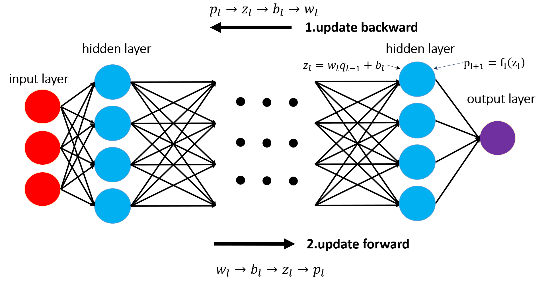
Figure 1: The overview of existing dlADMM algorithm: parameters are updated in a sequential fashion.

Notations	Descriptions
$L$	Number of layers.
$W_{l}$	The weight matrix for the $l$-th layer.
$b_{l}$	The intercept vector for the $l$-th layer.
$z_{l}$	The auxiliary variable of the linear mapping for the $l$-th layer.
$f_{l}(z_{l})$	The nonlinear activation function for the $l$-th layer.
$p_{l}$	The input for the $l$-th layer.
$q_{l}$	The output for the $l$-th layer.
$x$	The input matrix of the neural network.
$y$	The predefined label vector.
$R(z_{L},y)$	The risk function for the $l$-th layer.
$n_{l}$	The number of neurons for the $l$-th layer.

TABLE I: Important Notations

In this section, we introduce the formulation of the feed-forward neural network training problem and an existing deep learning ADMM method. The important notations of this paper are detailed in Table I.

The feed-forward neural network is formulated as follows [2]:

Problem 1.

$$\min\nolimits_{W_{l},b_{l},z_{l},p_{l}}R(z_{L};y)$$

$$s.t.\ z_{l}=W_{l}p_{l}+b_{l},\ p_{l+1}=f_{l}(z_{l})(l=1,\cdots,L-1)$$

where $p_{1}=x\in\mathbb{R}^{n_{0}}$ is the input of the deep neural network where $n_{0}$ is the number of feature dimensions, and $y$ is a predefined label vector. $p_{l}$ is the input for the $l$-th layer, also the output for the $(l-1)$-th layer. $R(z_{L};y)$ is a risk function for the $L$-th layer, which is convex, continuous and proper. $z_{l}=W_{l}p_{l}+b_{l}$ and $p_{l+1}=f_{l}(z_{l})$ are linear and nonlinear mappings for the $l$-th layer, respectively.
Problem 1 has been addressed by deep learning Alternating Direction Method of Multipliers (dlADMM) [2]. As shown in Figure 1, the dlADMM algorithm updates parameters from the final layer, and moves backward to the first layer, then updates parameters forward from the first layer to the final layer, in order to exchange information efficiently. However, parameters in one layer are dependent on its neighboring layers, and hence can not achieve parallelism. For example, the update of $p_{l+1}$ on the $l+1$-th layer needs to wait before $z_{l}$ on the $l$-th layer is updated. In order to address layer dependency, we relax Problem 1 to Problem 2 as follows:

Problem 2.

$$\min\nolimits_{\textbf{p},\textbf{W},\textbf{b},\textbf{z},\textbf{q}}F(\textbf{p},\textbf{W},\textbf{b},\textbf{z},\textbf{q})=R(z_{L};y)$$

$$+(\nu/2)(\sum\nolimits_{l=1}^{L}\|z_{l}-W_{l}p_{l}-b_{l}\|^{2}_{2}+\sum\nolimits_{l=1}^{L-1}\|q_{l}-f_{l}(z_{l})\|^{2}_{2})$$

$$s.t.\ p_{l+1}=q_{l}$$

where $\textbf{p}=\{p_{l}\}_{l=1}^{L}$, $\textbf{W}=\{W_{l}\}_{l=1}^{L}$, $\textbf{b}=\{b_{l}\}_{l=1}^{L}$, $\textbf{z}=\{z_{l}\}_{l=1}^{L}$, $\textbf{q}=\{q_{l}\}_{l=1}^{L-1}$, and $\nu>0$ is a tuning parameter. As $\nu\rightarrow\infty$, Problem 2 approaches Problem 1. We reduce layer dependency by splitting the output of the $l$-th layer and the input of the $l+1$-th layer into two variables $p_{l+1}$ and $q_{l}$, respectively.

The high-level overview of the pdADMM algorithm is shown in Figure 2. Specifically, by breaking the whole neural network into multiple layers, each of which can be optimized by an independent worker. Therefore, the layerwise training can be implemented in parallel. Moreover, the gradient vanishing problem can be avoided in this way. This is because the accumulate gradient calculated by the backpropagation algorithm is split into layerwise components.
Now we follow the ADMM routine to solve Problem 2, the augmented Lagrangian function is formulated mathematically as follows:

$$L_{\rho}(\textbf{p},\textbf{W},\textbf{b},\textbf{z},\textbf{q},\textbf{u})$$

$$=F(\textbf{p},\textbf{W},\textbf{b},\textbf{z},\textbf{q})+\sum\nolimits_{l\!=\!1}^{L\!-\!1}(u_{l}^{T}(p_{l\!+\!1}\!-\!q_{l})\!+\!(\rho/2)\|p_{l+1}-q_{l}\|^{2}_{2})$$

$$=\!R(z_{L};y)\!+\!\phi(p_{1},W_{1},b_{1},z_{1})\!+\!\sum\nolimits_{l\!=\!2}^{L}\!\phi(p_{l},W_{l},b_{l},z_{l},q_{l-1},u_{l\!-\!1})\!$$

$$+\!(\nu/2)\sum\nolimits_{l\!=\!1}^{L-1}\|q_{l}\!-\!f_{l}(z_{l})\|^{2}_{2}$$

where $\phi(p_{1},W_{1},b_{1},z_{1})=(\nu/2)\|z_{1}-W_{1}p_{1}-b_{1}\|^{2}_{2}$, $\phi(p_{l},W_{l},b_{l},z_{l},q_{l-1},u_{l-1})=(\nu/2)\|z_{l}-W_{l}p_{l}-b_{l}\|^{2}_{2}+u^{T}_{l-1}(p_{l}-q_{l-1})+(\rho/2)\|p_{l}-q_{l-1}\|^{2}_{2}$, $u_{l}(l=1,\cdots,L-1)$ are dual variables, $\rho>0$ is a parameter, and $\textbf{u}=\{u_{l}\}_{l=1}^{L-1}$. The detail of the pdADMM is shown in Algorithm 1. Specifically, Lines 5-9 update primal variables p, W, b, z and q, respectively, while Line 11 updates the dual variable u. the discussion on how to solve subproblems generated by pdADMM is detailed in the next section.

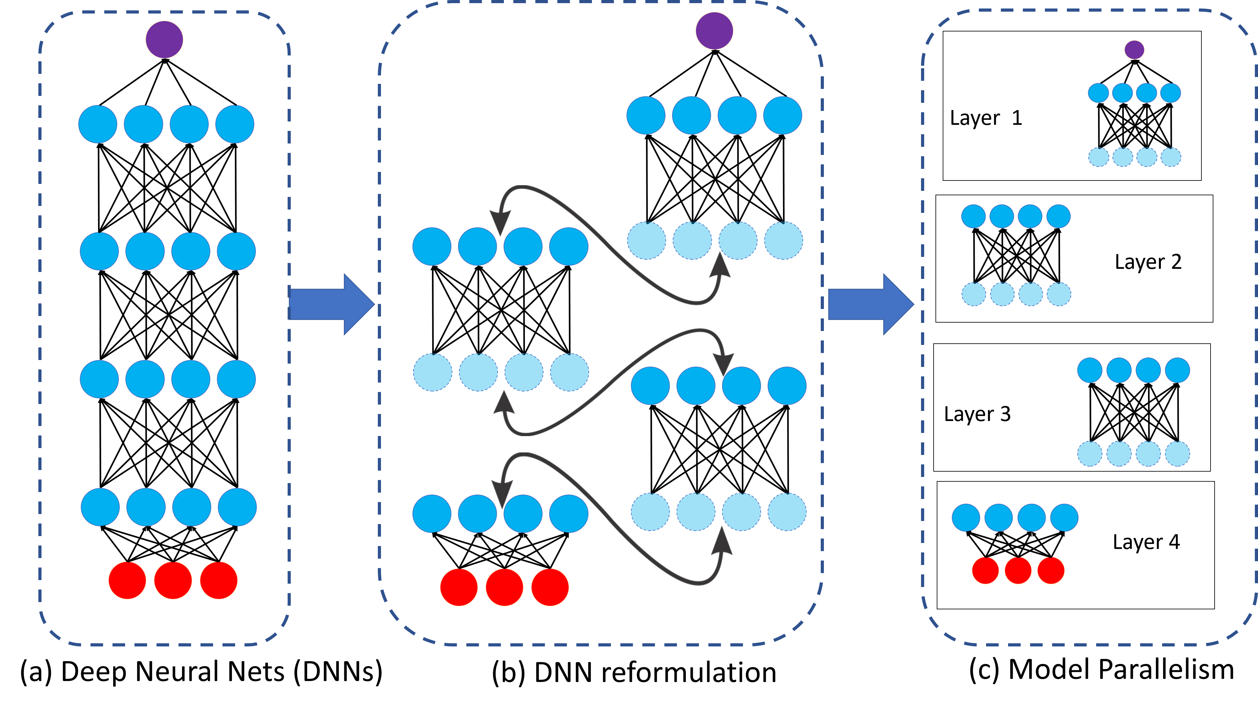
Figure 2: The pdADMM optimization framework: an overview

Algorithm 1 the pdADMM Algorithm

0:  $y$, $p_{1}=x$, $\rho$, $\nu$.

0:  $\textbf{p},\textbf{W},\textbf{b},\textbf{z},\textbf{q}$.

  Initialize $k=0$.

  while $\textbf{p}^{k},\textbf{W}^{k},\textbf{b}^{k},\textbf{z}^{k},\textbf{q}^{k}$ not converged do

     Update $p_{l}^{k+1}$ of different $l$ by Equation (1) in parallel.

     Update $W_{l}^{k+1}$ of different $l$ by Equation (2) in parallel.

     Update $b_{l}^{k+1}$ of different $l$ by Equation (3) in parallel.

     Update $z_{l}^{k+1}$ of different $l$ by Equations (4) and (5) in parallel.

     Update $q_{l}^{k+1}$ of different $l$ by Equation (6) in parallel.

     $r^{k}_{l}\leftarrow p^{k+1}_{l+1}-q^{k+1}_{l}(l=1,\cdots,L)$ in parallel # Compute residuals.

     Update $u_{l}^{k+1}$ of different $l$ by Equation (7) in parallel.

     $k\leftarrow k+1$.

  end while

  Output $\textbf{p},\textbf{W},\textbf{b},\textbf{z},\textbf{q}$.

III-B Solutions to All Subproblems

In this section, we discuss how to solve all subproblems generated by pdADMM in detail.
1. Update $\textbf{p}^{k+1}$
The variable $\textbf{p}^{k+1}$ is updated as follows:

$$p^{k+1}_{l} \leftarrow\arg\min\nolimits_{p_{l}}L_{\rho}(\textbf{p},\textbf{W}^{k},\textbf{b}^{k},\textbf{z}^{k},\textbf{q}^{k},\textbf{u}^{k})$$

$$=\phi(p_{l},W^{k}_{l},b^{k}_{l},z^{k}_{l},q^{k}_{l-1},u^{k}_{l-1})$$

Because $W_{l}$ and $p_{l}$ are coupled in $\phi$, solving $p_{l}$ should require the time-consuming operation of matrix inversion of $W_{l}$. To handle this, we apply similar quadratic approximation techniques as used in dlADMM [2] as follows:

$$p_{l}^{k+1} \leftarrow\arg\min_{p_{l}}U_{l}(p_{l};\tau_{l}^{k+1})$$ (1)

where $U_{l}(p_{l};\tau^{k+1}_{l})=\phi(p^{k}_{l},W^{k}_{l},b^{k}_{l},z^{k}_{l},q^{k}_{l-1},u^{k}_{l-1})+(\nabla_{p^{k}_{l}}\phi(p^{k}_{l},W^{k}_{l},b^{k}_{l},z^{k}_{l},q^{k}_{l-1},u^{k}_{l-1})(p_{l}-p^{k}_{l})+({\tau}^{k+1}_{l}/2)\|p_{l}-p^{k}_{l}\|^{2}_{2}$, and $\tau^{k+1}_{l}>0$ is a parameter. $\tau_{l}^{k+1}$ should satisfy $\phi(p^{k+1}_{l},W^{k}_{l},b^{k}_{l},z^{k}_{l},q^{k}_{l-1},u^{k}_{l-1})\leq U_{l}(p^{k+1}_{l};\tau^{k+1}_{l})$. The solution to Equation (1) is: ${p}^{k+1}_{l}\leftarrow p^{k}_{l}-\nabla_{p^{k}_{l}}\phi(p^{k}_{l},W^{k}_{l},b^{k}_{l},z^{k}_{l},q^{k}_{l-1},u^{k}_{l-1})/{\tau}^{k+1}_{l}$.
2. Update $\textbf{W}^{k+1}$
The variable $\textbf{W}^{k+1}$ is updated as follows:

$$W^{k+1}_{l} \leftarrow\arg\min\nolimits_{W_{l}}L_{\rho}(\textbf{p}^{k+1},\textbf{W},\textbf{b}^{k},\textbf{z}^{k},\textbf{q}^{k},\textbf{u}^{k})$$

$$=\arg\min\nolimits_{W_{l}}\begin{cases}\phi(p^{k+1}_{1},W_{1},b^{k}_{1},z^{k}_{1})&l=1\\ \phi(p^{k\!+\!1}_{l},W_{l},b^{k}_{l},z^{k}_{l},q^{k}_{l\!-\!1},u^{k}_{l\!-\!1})&1<\!l\!\leq\!L\end{cases}$$

Similar to updating $p_{l}$, the following subproblem should be solved instead:

$$W_{l}^{k+1} \leftarrow\arg\min\nolimits_{W_{l}}V_{l}(W_{l};\theta_{l}^{k+1})$$ (2)

where

$$V_{1}(W_{1};\theta^{k+1}_{1})=\phi(p^{k+1}_{1},W^{k}_{1},b^{k}_{1},z^{k}_{1})$$

$$+\!\nabla_{W^{k}_{1}}\phi^{T}(p^{k+1}_{1},W^{k}_{1},b^{k}_{1},z^{k}_{1})(W_{1}\!-\!W^{k}_{1})$$

$$+({\theta}^{k+1}_{l}/2)\|W_{1}-W^{k}_{1}\|^{2}_{2}$$

$$V_{l}(W_{l};\theta^{k+1}_{l})=\phi(p^{k+1}_{l},W^{k}_{l},b^{k}_{l},z^{k}_{l},q^{k}_{l-1},u^{k}_{l-1})$$

$$+\nabla_{W^{k}_{l}}\phi^{T}(p^{k+1}_{l},W^{k}_{l},b^{k}_{l},z^{k}_{l},q^{k}_{l-1},u^{k}_{l-1})(W_{l}-W^{k}_{l})$$

$$+({\theta}^{k+1}_{l}/2)\|W_{l}-W^{k}_{l}\|^{2}_{2}$$

and $\theta^{k+1}_{l}$ is a parameter, which should satisfy $\phi(p^{k+1}_{1},W^{k+1}_{1},b^{k}_{1},z^{k}_{1})\leq V(W^{k+1}_{1};\theta^{k+1}_{1})$ and $\phi(p^{k+1}_{l},W^{k+1}_{l},b^{k}_{l},z^{k}_{l},q^{k}_{l-1},u^{k}_{l-1})\leq V(W^{k+1}_{l};\theta^{k+1}_{l})(1<l<L)$. The solution to Equation (2) is shown as follows:

$${W}^{k\!+\!1}_{l}\!\leftarrow\!W^{k}_{l}\!-\!\begin{cases}\nabla_{W^{k}_{1}}\phi(p^{k+1}_{1}\!,\!W^{k}_{1}\!,\!b^{k}_{1}\!,\!z^{k}_{1})/\theta^{k+1}_{l}&l=1\\ \nabla_{W^{k}_{l}}\phi(p^{k\!+\!1}_{l}\!,\!W^{k}_{l}\!,\!b^{k}_{l}\!,\!z^{k}_{l}\!,\!q^{k}_{l\!-\!1}\!,\!u^{k}_{l\!-\!1})/\theta^{k\!+\!1}_{l}&1\!<l\!\leq\!L\end{cases}$$

3. Update $\textbf{b}^{k+1}$
The variable $\textbf{b}^{k+1}$ is updated as follows:

$$b^{k+1}_{l} \leftarrow\arg\min\nolimits_{b_{l}}L_{\rho}(\textbf{p}^{k+1},\textbf{W}^{k+1},\textbf{b},\textbf{z}^{k},\textbf{q}^{k},\textbf{u}^{k})$$

$$=\arg\min\nolimits_{b_{l}}\begin{cases}\phi(p^{k+1}_{1},W^{k+1}_{1},b_{1},z^{k}_{1})&l\!=\!1\\ \phi(p^{k+1}_{l},W^{k\!+\!1}_{l},b_{l},z^{k}_{l},q^{k}_{l\!-\!1},u^{k}_{l\!-\!1})&1<\!l\!\leq L\end{cases}.$$

Similarly, we solve the following subproblems instead:

$$b^{k+1}_{1}\leftarrow\arg\min\nolimits_{b_{1}}\phi(p^{k+1}_{1},W^{k+1}_{1},b^{k}_{1},z^{k}_{1})$$

$$+\nabla_{b^{k}_{1}}\phi^{T}(p^{k+1}_{1},W^{k+1}_{1},b^{k}_{1},z^{k}_{1})(b_{l}-b^{k}_{l})+(\nu/2)\|b_{l}-b^{k}_{l}\|^{2}_{2}$$

$$b^{k+1}_{l}\leftarrow\arg\min\nolimits_{b_{l}}\phi(p^{k+1}_{l},W^{k+1}_{l},b^{k}_{l},z^{k}_{l},q^{k}_{l-1},u^{k}_{l-1})$$

$$+\nabla_{b^{k}_{l}}\phi^{T}(p^{k+1}_{l},W^{k+1}_{l},b^{k}_{l},z^{k}_{l},q^{k}_{l-1},u^{k}_{l-1})(b_{l}-b^{k}_{l})$$

$$+(\nu/2)\|b_{l}-b^{k}_{l}\|^{2}_{2}(1<l\leq L)$$ (3)

The solution to Equation (3) is:

$${b}^{k\!+\!1}_{l}\leftarrow b^{k}_{l}\!-\!\begin{cases}\nabla_{b^{k}_{1}}\phi(p^{k\!+\!1}_{1},W^{k\!+\!1}_{1},b^{k}_{1},z^{k}_{1})/\nu&l=1\\ \nabla_{b^{k}_{l}}\phi(p^{k\!+\!1}_{l},W^{k\!+\!1}_{l},b^{k}_{l},z^{k}_{l},q^{k}_{l\!-\!1},u^{k}_{l\!-\!1})/\nu&1\!<\!l\!\leq L\end{cases}$$

4. Update $\textbf{z}^{k+1}$
The variable $\textbf{z}^{k+1}$ is updated as follows:

$$z^{k\!+\!1}_{l}\!\leftarrow\!\arg\min\nolimits_{z_{l}}(\nu/2)\|z_{l}\!-\!W^{k\!+\!1}_{l}\!p^{k\!+\!1}_{l}\!-\!b^{k\!+\!1}_{l}\|^{2}_{2}$$

$$+\!(\nu/2)\|q^{k}_{l}\!-\!f_{l}(z_{l})\|^{2}_{2}\!+\!(\nu/2)\|z_{l}\!-\!z^{k}_{l}\|^{2}_{2}(l\!<\!L)$$ (4)

$$z^{k\!+\!1}_{L}\!\leftarrow\!\arg\min\nolimits_{z_{l}}\!R(z_{L};y)\!+\!(\nu/2)\!\|z_{L}\!-\!W^{k\!+\!1}_{L}p^{k\!+\!1}_{L}\!-\!b^{k\!+\!1}_{L}\|^{2}_{2}\!$$ (5)

where a quadratic term $(\nu/2)\|z_{l}-z^{k}_{l}\|^{2}_{2}$ is added in Equation (4) to control $z^{k+1}_{l}$ to close to $z^{k}_{l}$. Equation (5) is convex, which can be solved by Fast Iterative Soft Thresholding Algorithm (FISTA) [41].
For Equation (4), nonsmooth activations usually lead to closed-form solutions [2, 22]. For example, for Relu $f_{l}(z_{l})=\max(z_{l},0)$, the solution to Equation (4) is shown as follows:

$$z^{k+1}_{l}=\begin{cases}\min((W^{k\!+\!1}_{l}p^{k\!+\!1}_{l}\!+\!b^{k+1}_{l}\!+\!z^{k}_{l})/2,0)&z^{k\!+\!1}_{l}\leq 0\\ \max((W^{k\!+\!1}_{l}p^{k\!+\!1}_{l}\!+\!b^{k\!+\!1}_{l}\!+\!q^{k}_{l}\!+\!z^{k}_{l})/3,0)&z^{k+1}_{l}\geq 0\\ \end{cases}$$

For smooth activations such as tanh and sigmoid, a lookup-table is recommended [2].
5. Update $\textbf{q}^{k+1}$
The variable $\textbf{q}^{k+1}$ is updated as follows:

$$q^{k+1}_{l} \leftarrow\arg\min\nolimits_{q_{l}}L_{\rho}(\textbf{p}^{k+1},\textbf{W}^{k+1},\textbf{b}^{k+1},\textbf{z}^{k+1},\textbf{q},\textbf{u}^{k})$$

$$=\arg\min\nolimits_{q_{l}}\phi(p^{k+1}_{l+1},W^{k+1}_{l+1},b^{k+1}_{l+1},z^{k+1}_{l+1},q_{l},u^{k}_{l}).$$ (6)

Equation (6) has a closed-form solution as follows:

$$q^{k+1}_{l}\leftarrow(\rho p_{l+1}^{k+1}+u^{k}_{l}+\nu f_{l}(z^{k+1}_{l}))/(\rho+\nu)$$

6. Update $\textbf{u}^{k+1}$
The variable $\textbf{u}^{k+1}$ is updated as follows:

$$u^{k+1}_{l} \leftarrow u^{k}_{l}+\rho(p^{k+1}_{l+1}-q^{k+1}_{l})$$ (7)

Finally, Our proposed pdADMM can be efficient for training a deep feed-forward neural network. To achieve this, we begin from training a swallow neural network with the first few layers of the deep neural network, then more layers are added for training step by step until finally all layers are involved in the training process. The pdADMM can achieve good performance as well as reduce training cost by this strategy.

IV Convergence Analysis

In this section, the theoretical convergence of the proposed pdADMM algorithm. Firstly, the Lipschitz continuity and coercivity are defined as follows:

Definition 1.

(Lipschitz Continuity) A function $g(x)$ is Lipschitz continuous if there exists a constant $D>0$ such that $\forall x_{1},x_{2}$, the following holds

$$\|g(x_{1})-g(x_{2})\|\leq D\|x_{1}-x_{2}\|.$$

Definition 2.

(Coercivity) A function $h(x)$ is coerce over the feasible set $\mathscr{F}$ means that $h(x)\rightarrow\infty$ if $x\in\mathscr{F}$ and $\|x\|\rightarrow\infty$.

Then the following assumption is required for convergence analysis.

Assumption 1.

$f_{l}(z_{l})$ is Lipschitz continuous with coefficient $S>0$, and $F(\textbf{p},\textbf{W},\textbf{b},\textbf{z},\textbf{q})$ is coercive. Moreover, $\partial f_{l}(z_{l})$ is bounded, i.e. there exists $M>0$ such that $\|\partial f_{l}(z_{l})\|\leq M$.

Assumption 1 is mild to satisfy: most common activation functions such as Relu and leaky Relu satisfy Assumption 1. No assumption is needed on the risk function $R(z_{l};y)$, which shows that the convergence condition of our proposed pdADMM is milder than that of the dlADMM, which requires $R(z_{l};y)$ to be Lipschitz differentiable [2]. Due to space limit, the detailed proofs are provided in the Appendix. The technical proofs follow the similar routine as dlADMM [2]. The difference consists in the fact that the dual variable $u_{l}$ is controlled by $q_{l}$ and $z_{l}$ (Lemma 6 in the Appendix), which holds under Assumption 1, while $u_{l}$ can be controlled only by $z_{l}$ in the convergence proof of dlADMM. The first lemma shows that the objective keeps decreasing when $\rho$ is sufficently large.

Lemma 1 (Decreasing Objective).

If $\rho>\max(4\nu S^{2},(\sqrt{17}+1)\nu/2)$, there exist $C_{1}=\nu/2-2\nu^{2}S^{2}/\rho>0$ and $C_{2}=\rho/2-2\nu^{2}/\rho-\nu/2>0$ such that it holds for any $k\in\mathbb{N}$ that

$$L_{\rho}(\textbf{p}^{k},\textbf{W}^{k},\textbf{b}^{k},\textbf{z}^{k},\textbf{q}^{k},\textbf{u}^{k})\!-\!L_{\rho}(\textbf{p}^{k\!+\!1},\textbf{W}^{k\!+\!1},\textbf{b}^{k\!+\!1},\textbf{z}^{k\!+\!1},\textbf{q}^{k\!+\!1},\textbf{u}^{k\!+\!1})$$

$$\geq\sum\nolimits_{l\!=\!2}^{L}(\tau^{k\!+\!1}_{l}/2)\|p^{k+1}_{l}\!-\!p^{k}_{l}\|^{2}_{2}\!+\!\sum\nolimits_{l\!=\!1}^{L}(\theta^{k\!+\!1}_{l}/2)\|W^{k\!+\!1}_{l}\!-\!W^{k}_{l}\|^{2}_{2}\!$$

$$+\!\sum\nolimits_{l\!=\!1}^{L}(\nu/2)\|b^{k\!+\!1}_{l}\!-\!b^{k}_{l}\|^{2}_{2}\!+\!\sum\nolimits_{l\!=\!1}^{L\!-\!1}C_{1}\|z^{k+1}_{l}\!-\!z^{k}_{l}\|^{2}_{2}$$

$$\!+\!(\nu/2)\|z^{k+1}_{L}-z^{k}_{L}\|^{2}_{2}+\sum\nolimits_{l=1}^{L-1}C_{2}\|q^{k+1}_{l}-q^{k}_{l}\|^{2}_{2}$$ (8)

The second Lemma illustrates that the objective is bounded from below when $\rho$ is large enough, and all variables are bounded.

Lemma 2 (Bounded Objective).

If $\rho>\nu$, then $L_{\rho}(\textbf{p}^{k},\textbf{W}^{k},\textbf{b}^{k},\textbf{z}^{k},\textbf{q}^{k},\textbf{u}^{k})$ is lower bounded. Moreover, $\textbf{p}^{k},\textbf{W}^{k},\textbf{b}^{k},\textbf{z}^{k},\textbf{q}^{k}$,and $\textbf{u}^{k}$ are bounded, i.e. there exist $\mathbb{N}_{\textbf{p}}$, $\mathbb{N}_{\textbf{W}}$, $\mathbb{N}_{\textbf{b}}$, $\mathbb{N}_{\textbf{z}}$, $\mathbb{N}_{\textbf{q}}$, and $\mathbb{N}_{\textbf{u}}>0$, such that $\|\textbf{p}^{k}\|\leq\mathbb{N}_{\textbf{p}}$, $\|\textbf{W}^{k}\|\leq\mathbb{N}_{\textbf{W}}$, $\|\textbf{b}^{k}\|\leq\mathbb{N}_{\textbf{b}}$, $\|\textbf{z}^{k}\|\leq\mathbb{N}_{\textbf{z}}$, $\|\textbf{q}^{k}\|\leq\mathbb{N}_{\textbf{q}}$, and $\|\textbf{u}^{k}\|\leq\mathbb{N}_{\textbf{u}}$.

Based on Lemmas 1 and 2, the following theorem ensures that the objective is convergent.

Theorem 1 (Convergent Objective).

If $\rho>\max(4\nu S^{2},(\sqrt{17}+1)\nu/2)$, then $L_{\rho}(\textbf{p}^{k},\textbf{W}^{k},\textbf{b}^{k},\textbf{z}^{k},\textbf{q}^{k},\textbf{u}^{k})$ is convergent. Moreover, $\lim_{k\rightarrow\infty}\|\textbf{p}^{k+1}-\textbf{p}^{k}\|^{2}_{2}=0$, $\lim_{k\rightarrow\infty}\|\textbf{W}^{k+1}-\textbf{W}^{k}\|^{2}_{2}=0$, $\lim_{k\rightarrow\infty}\|\textbf{b}^{k+1}-\textbf{b}^{k}\|^{2}_{2}=0$, $\lim_{k\rightarrow\infty}\|\textbf{z}^{k+1}-\textbf{z}^{k}\|^{2}_{2}=0$, $\lim_{k\rightarrow\infty}\|\textbf{q}^{k+1}-\textbf{q}^{k}\|^{2}_{2}=0$, $\lim_{k\rightarrow\infty}\|\textbf{u}^{k+1}-\textbf{u}^{k}\|^{2}_{2}=0$.

Proof.

From Lemmas 1 and 2, we know that $L_{\rho}(\textbf{p}^{k},\textbf{W}^{k},\textbf{b}^{k},\textbf{z}^{k},\textbf{q}^{k},\textbf{u}^{k})$ is convergent because a monotone bounded sequence converges. Moreover, we take the limit on the both sides of Inequality (8) to obtain

$$0=\lim\nolimits_{k\rightarrow\infty}L_{\rho}(\textbf{p}^{k},\textbf{W}^{k},\textbf{b}^{k},\textbf{z}^{k},\textbf{q}^{k},\textbf{u}^{k})$$

$$-\lim\nolimits_{k\rightarrow\infty}L_{\rho}(\textbf{p}^{k+1},\textbf{W}^{k+1},\textbf{b}^{k+1},\textbf{z}^{k+1},\textbf{q}^{k+1},\textbf{u}^{k+1})$$

$$\geq\lim\nolimits_{k\rightarrow\infty}(\sum\nolimits_{l=2}^{L}(\tau^{k+1}_{l}/2)\|p^{k+1}_{l}\!-\!p^{k}_{l}\|^{2}_{2}$$

$$+\sum\nolimits_{l\!=\!1}^{L}(\theta^{k\!+\!1}_{l}/2)\|W^{k\!+\!1}_{l}\!-\!W^{k}_{l}\|^{2}_{2}+\sum\nolimits_{l\!=\!1}^{L}(\nu/2)\|b^{k\!+\!1}_{l}\!-\!b^{k}_{l}\|^{2}_{2}$$

$$+\sum\nolimits_{l=1}^{L-1}C_{1}\|z^{k+1}_{l}-z^{k}_{l}\|^{2}_{2}+(\nu/2)\|z^{k+1}_{L}-z^{k}_{L}\|^{2}_{2}$$

$$+\sum\nolimits_{l=1}^{L-1}C_{2}\|q^{k+1}_{l}-q^{k}_{l}\|^{2}_{2})\geq 0$$

Because $L_{\rho}(\textbf{p}^{k},\textbf{W}^{k},\textbf{b}^{k},\textbf{z}^{k},\textbf{q}^{k},\textbf{u}^{k})$ is convergent, then $\lim_{k\rightarrow\infty}\|\textbf{p}^{k+1}-\textbf{p}^{k}\|^{2}_{2}=0$, $\lim_{k\rightarrow\infty}\|\textbf{W}^{k+1}-\textbf{W}^{k}\|^{2}_{2}=0$, $\lim_{k\rightarrow\infty}\|\textbf{b}^{k+1}-\textbf{b}^{k}\|^{2}_{2}=0$, $\lim_{k\rightarrow\infty}\|\textbf{z}^{k+1}-\textbf{z}^{k}\|^{2}_{2}=0$, and $\lim_{k\rightarrow\infty}\|\textbf{q}^{k+1}-\textbf{q}^{k}\|^{2}_{2}=0$. $\lim_{k\rightarrow\infty}\|\textbf{u}^{k+1}-\textbf{u}^{k}\|^{2}_{2}=0$ is derived from Lemma 6 in the Appendix. ∎

The third lemma guarantees that the subgradient of the objective is upper bounded, which is stated as follows:

Lemma 3 (Bounded Subgradient).

There exists a constant $C>0$ and $g^{k+1}\in\partial L_{\rho}(\textbf{p}^{k+1},\textbf{W}^{k+1},\textbf{b}^{k+1},\textbf{z}^{k+1},\textbf{q}^{k+1},\textbf{u}^{k+1})$ such that

$$\|g^{k+1}\|\leq C(\|\textbf{p}^{k+1}-\textbf{p}^{k}\|+\|\textbf{W}^{k+1}-\textbf{W}^{k}\|+\|\textbf{b}^{k+1}-\textbf{b}^{k}\|$$

$$+\|\textbf{z}^{k+1}-\textbf{z}^{k}\|+\|\textbf{q}^{k+1}-\textbf{q}^{k}\|+\|\textbf{u}^{k+1}-\textbf{u}^{k}\|)$$

Now based on Theorem 1, and Lemma 3, the convergence of the pdADMM algorithm to a critical point is presented in the following theorem.

Theorem 2 (Convergence to a Critical Point).

If $\rho>\max(4\nu S^{2},(\sqrt{17}+1)\nu/2)$, then for the variables $(\textbf{p},\textbf{W},\textbf{b},\textbf{z},\textbf{q},\textbf{u})$ in Problem 2, starting from any $(\textbf{p}^{0},\textbf{W}^{0},\textbf{b}^{0},\textbf{z}^{0},\textbf{q}^{0},\textbf{u}^{0})$, $(\textbf{p}^{k},\textbf{W}^{k},\textbf{b}^{k},\textbf{z}^{k},\textbf{q}^{k},\textbf{u}^{k})$ has at least a limit point $(\textbf{p}^{*},\textbf{W}^{*},\textbf{b}^{*},\textbf{z}^{*},\textbf{q}^{*},\textbf{u}^{*})$, and any limit point is a critical point of Problem 2. That is, $0\in\partial L_{\rho}(\textbf{p}^{*},\textbf{W}^{*},\textbf{b}^{*},\textbf{z}^{*},\textbf{q}^{*},\textbf{u}^{*})$. In other words,

$$p^{*}_{l+1}=q^{*}_{l},\ \nabla_{\textbf{p}^{*}}L_{\rho}(\textbf{p}^{*},\textbf{W}^{*},\textbf{b}^{*},\textbf{z}^{*},\textbf{q}^{*},\textbf{u}^{*})=0,$$

$$\ \nabla_{\textbf{W}^{*}}L_{\rho}(\textbf{p}^{*},\textbf{W}^{*},\textbf{b}^{*},\textbf{z}^{*},\textbf{q}^{*},\textbf{u}^{*})=0,$$

$$\nabla_{\textbf{b}^{*}}L_{\rho}(\textbf{p}^{*},\textbf{W}^{*},\textbf{b}^{*},\textbf{z}^{*},\textbf{q}^{*},\textbf{u}^{*})=0,$$

$$0\in\partial_{\textbf{z}^{*}}L_{\rho}(\textbf{p}^{*},\textbf{W}^{*},\textbf{b}^{*},\textbf{z}^{*},\textbf{q}^{*},\textbf{u}^{*}),$$

$$\nabla_{\textbf{q}^{*}}L_{\rho}(\textbf{p}^{*},\textbf{W}^{*},\textbf{b}^{*},\textbf{z}^{*},\textbf{q}^{*},\textbf{u}^{*})=0.$$

Proof.

From Lemma 2, $(\textbf{p}^{k},\textbf{W}^{k},\textbf{b}^{k},\textbf{z}^{k},\textbf{q}^{k},\textbf{u}^{k})$ has at least a limit point $(\textbf{p}^{*},\textbf{W}^{*},\textbf{b}^{*},\textbf{z}^{*},\textbf{q}^{*},\textbf{u}^{*})$ because a bounded sequence has at least a limit point. From Lemma 3 and Theorem 1, $\|g^{k+1}\|\rightarrow 0$ as $k\rightarrow\infty$. According to the definition of general subgradient (Defintion 8.3 in [42]), we have $0\in\partial L_{\rho}(\textbf{p}^{*},\textbf{W}^{*},\textbf{b}^{*},\textbf{z}^{*},\textbf{q}^{*},\textbf{u}^{*})$. In other words, every limit point $(\textbf{p}^{*},\textbf{W}^{*},\textbf{b}^{*},\textbf{z}^{*},\textbf{q}^{*},\textbf{u}^{*})$ is a critical point. ∎

Theorem 2 shows that our proposed pdADMM algorithm converges for sufficiently large $\rho$, which is consistent with previous literature [2]. Next, the following theorem ensures the sublinear convergence rate $o(1/k)$ of the proposed pdADMM algorithm, whose proof is at the end of this paper.

Theorem 3 (Convergence Rate).

For a sequence $(\textbf{p}^{k},\textbf{W}^{k},\textbf{b}^{k},\textbf{z}^{k},\textbf{q}^{k},\textbf{u}^{k})$, define $c_{k}=\min\nolimits_{0\leq i\leq k}(\sum\nolimits_{l=2}^{L}(\tau^{i+1}_{l}/2)\|p^{i+1}_{l}\!-\!p^{i}_{l}\|^{2}_{2}+\sum\nolimits_{l\!=\!1}^{L}(\theta^{i\!+\!1}_{l}/2)\|W^{i\!+\!1}_{l}\!-\!W^{i}_{l}\|^{2}_{2}+\sum\nolimits_{l\!=\!1}^{L}(\nu/2)\|b^{i\!+\!1}_{l}\!-\!b^{i}_{l}\|^{2}_{2}+\sum\nolimits_{l=1}^{L-1}C_{1}\|z^{i+1}_{l}-z^{i}_{l}\|^{2}_{2}+(\nu/2)\|z^{i+1}_{L}-z^{i}_{L}\|^{2}_{2}+\sum\nolimits_{l=1}^{L-1}C_{2}\|q^{i+1}_{l}-q^{i}_{l}\|^{2}_{2})$ where $C_{1}=\nu/2-2\nu^{2}S^{2}/\rho>0$ and $C_{2}=\rho/2-2\nu^{2}/\rho-\nu/2>0$, then the convergence rate of $c_{k}$ is $o(1/k)$.

V Experiments

In this section, we evaluate the performance of the proposed pdADMM using six benchmark datasets. Speedup, convergence and accuracy performance are compared with several state-of-the-art optimizers. All experiments were conducted on 64-bit machine with Intel Xeon(R) silver 4114 Processor and 48GB RAM.

V-A Datasets

In this experiment, six benchmark datasets were used for performance evaluation:
1. MNIST [43]. The MNIST dataset has ten classes of handwritten-digit images, which was firstly introduced by Lecun et al. in 1998 [43]. It contains 55,000 training samples and 10,000 test samples with 196 features each, which is provided by the Keras library [44].
2. Fashion MNIST [45]. The Fashion MNIST dataset has ten classes of assortment images on the website of Zalando, which is Europe’s largest online fashion platform [45]. The Fashion-MNIST dataset consists of 60,000 training samples and 10,000 test samples with 196 features each.
3. kMNIST(Kuzushiji-MNIST) [46]. The kMNIST dataset has ten classes, each of which is a character to represent each of the 10 rows of Hiragana. The kMNIST dataset consists of 60,000 training samples and 10,000 test samples with 196 features each.
4. SVHN (Street View House Numbers) [47]. The SVHN dataset is obtained from house numbers in Google Street View images. It consists of ten classes of digits. In our experiments, we use three classes ’0’, ’1’ and ’2’. The number of training data and test data are 24,446 and 9,248, respectively, with 768 features each.
5. CIFAR10 [48]. CIFAR10 is a collection of color images with 10 different classes. In our experiments, we use two classes ’0’ and ’6’. The number of training data and test data are 12,000 and 2,000, respectively, with 768 features each.
6. CIFAR100 [48]. CIFAR100 is similar to CIFAR10 except that CIFAR100 has 100 classes. In our experiments, we use two classes ’0’ and ’2’. The number of training data and test data are 5,000 and 1,000, respectively, with 768 features each.

V-B Speedup

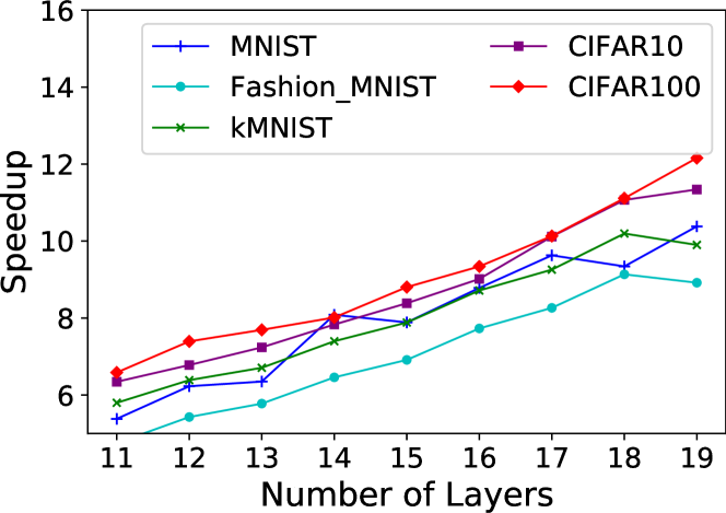
Figure 3: The relationship between speedup and the number of layers: the speedup increases linearly with the number of layers.

MNIST dataset
Neurons$\#$	Serial pdADMM (sec)	pdADMM(sec)	Speedup
1500	237.66	26.78	8.87
1600	348.70	31.78	10.97
1700	390.51	35.79	10.91
1800	475.60	41.37	11.50
1900	465.57	45.87	10.15
2000	570.90	50.70	11.26
2000	570.9	50.7	11.26
2100	570	54.91	10.38
2200	678.83	63.59	10.68
2300	710.3	70.36	10.10
2400	766.82	62.5	12.27
Fashion MNIST dataset
Neurons$\#$	Serial pdADMM (sec)	pdADMM(sec)	Speedup
1500	358.68	32.65	10.99
1600	407.71	37.90	10.76
1700	476.79	44.75	10.65
1800	539.51	50.50	10.68
1900	599.42	53.88	11.13
2000	645.87	58.68	11.01
2100	740.39	67.91	10.90
2200	818.58	74.17	11.03
kMNIST dataset
Neurons$\#$	Serial pdADMM (sec)	pdADMM(sec)	Speedup
1500	354.85	32.65	10.87
1600	407.73	37.11	10.99
1700	472.4648	42.58	11.10
1800	539.52	48.78	11.06
1900	596.84	55.56	10.74
2000	660.58	56.10	11.78
2100	737.78	66.95	11.02
2200	806.74	76.16	10.59
CIFAR10 dataset
Neurons$\#$	Serial pdADMM (sec)	pdADMM(sec)	Speedup
1500	326.62	25.00	13.06
1600	374.82	28.96	12.94
1700	433.46	33.99	12.75
1800	485.86	38.66	12.57
1900	544.11	43.10	12.62
2000	572.33	46.90	12.20
2100	602.65	55.25	10.91
2200	732.79	59.27	12.36
2300	784.87	56.26	13.95
2400	854.47	63.1	13.54
CIFAR100 dataset
Neurons$\#$	Serial pdADMM (sec)	pdADMM(sec)	Speedup
1500	334.55	25.39	13.18
1600	382.24	29.3	13.05
1700	445.23	34	13.09
1800	500.00	38.38	13.03
1900	549.77	43.25	12.71
2000	576.10	42.47	13.56
2100	666.06	47.43	14.04
2200	735.63	52.41	14.04
2300	793.03	56.73	13.98
2400	857.41	62.3	13.76

TABLE II: The relation between speedup and number of neurons on the MNIST, Fashion MNIST datasets, kMNIST, CIFAR10 and CIFAR100 datasets: the pdADMM runs 10 times faster than its serial version.

In this experiment, we investigate the speedup of the proposed pdADMM algorithm concerning the number of layers and the number of neurons on the large-scale deep neural networks. The activation function was set to the Rectified linear unit (Relu). The loss function was the cross-entropy loss. The running time per epoch was the average of 10 epochs. $\rho$ and $\nu$ were both set to $10^{-4}$.
Firstly, we investigated the relationship between speedup and the number of layers. We set up a feed-forward neural network with different number of hidden layers, which ranges from 11 to 19. The number of neurons in each layer was fixed to 2,400. The SVHN dataset was not tried due to memory issues. Figure 3 shows that the speedup increases linearly with the number of layers. Specifically, the speedup reached 11 when 19 hidden layers were trained. This indicates that the deeper a neural network is, the more speedup our proposed pdADMM can gain.
Secondly, the relationship between speedup and the number of neurons was studied. Specifically, we test our proposed pdADMM algorithm on a feed-forward neural network with 19 hidden layers. The number of neurons in each layer ranges from 1,500 to 2,400. The speedup was shown in Table II on the MNIST and Fashion MNIST datasets. Specifically, the speedup remains stable around $10$ no matter how many neurons were trained. This concludes that the speedup of the proposed pdADMM is independent of the number of neurons.

V-C Convergence

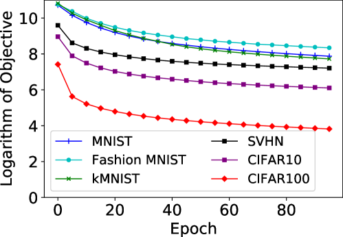
(a). Objective versus epoch

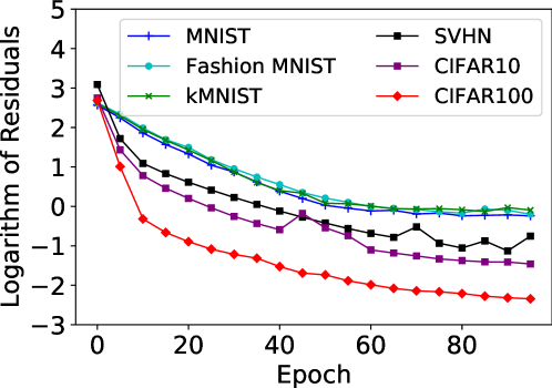
(b). Residual versus epoch

Figure 4: The convergence of the proposed pdADMM: the objective decreases monotonously, and the residual converges to 0.

To validate the convergence of the proposed pdADMM, we set up a feed-forward neural network with 9 hidden layers, each of which has 500 neurons. The Rectified linear unit (ReLU) was used for the activation function for both network structures. The loss function was set as the cross-entropy loss. The number of epoch was set to $100$. $\nu$ and $\rho$ were both set to $0.1$. As shown in Figure 4, the objective keeps decreasing monotonically on all six datasets, and the residual converges sublinearly to 0, which are consistent with Theorems 2 and 3.

V-D Accuracy

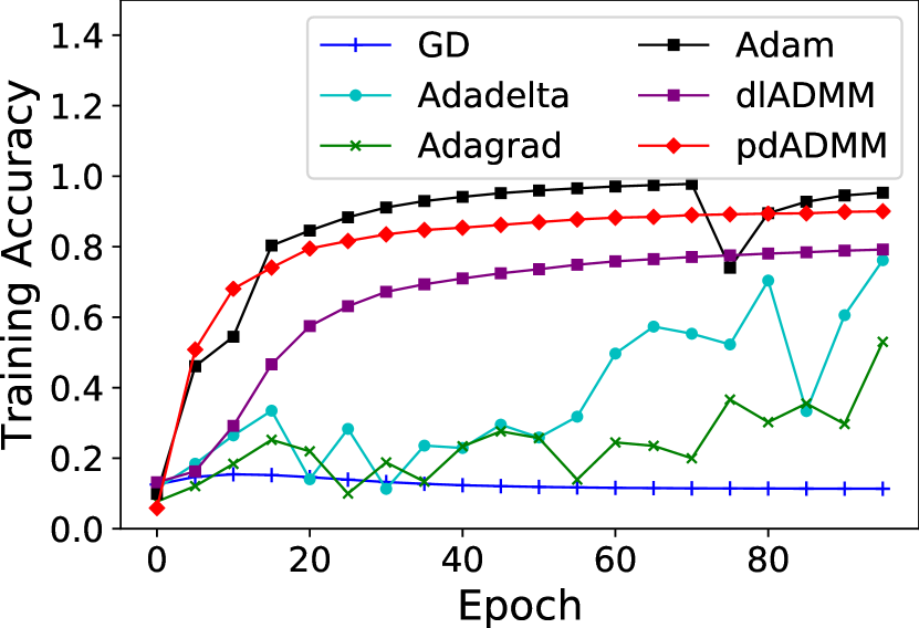
(a). MNIST

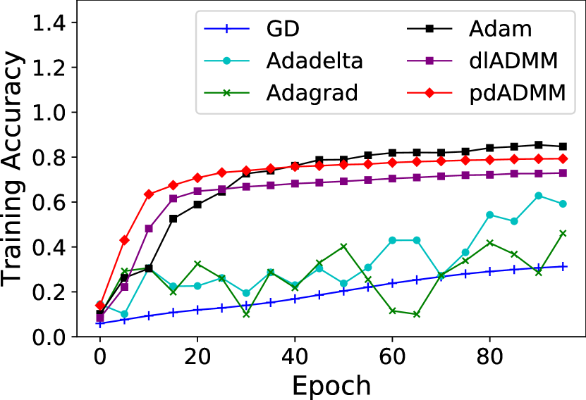
(b). Fashion MNIST

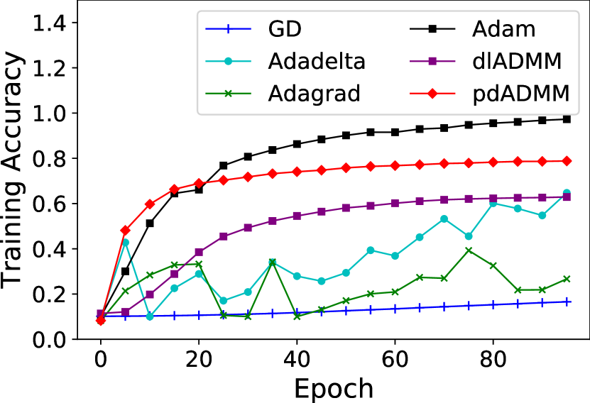
(c). kMNIST

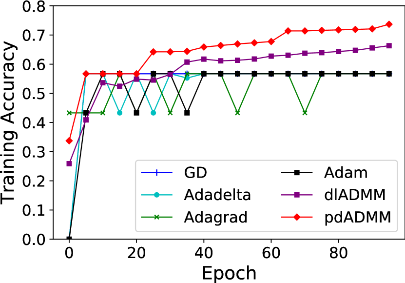
(d). SVHN

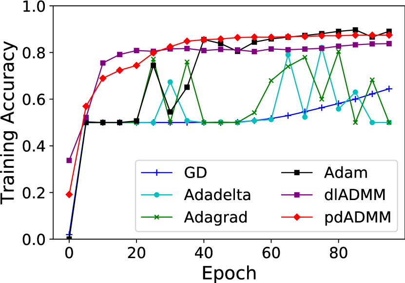
(e). CIFAR10

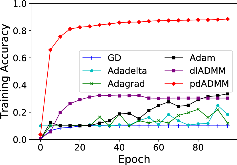
(f). CIFAR100

Figure 5: Training Accuracy of all methods: pdADMM outperformed most comparison methods; SGD-type methods suffer from gradient vanishing problems.

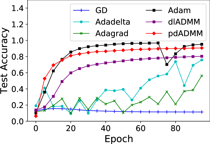
(a). MNIST

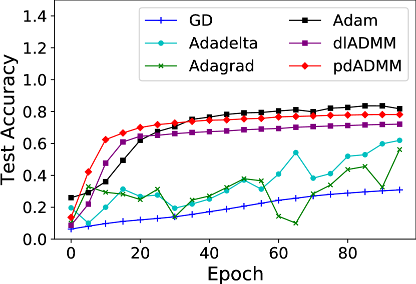
(b). Fashion MNIST

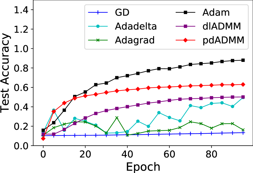
(c). kMNIST

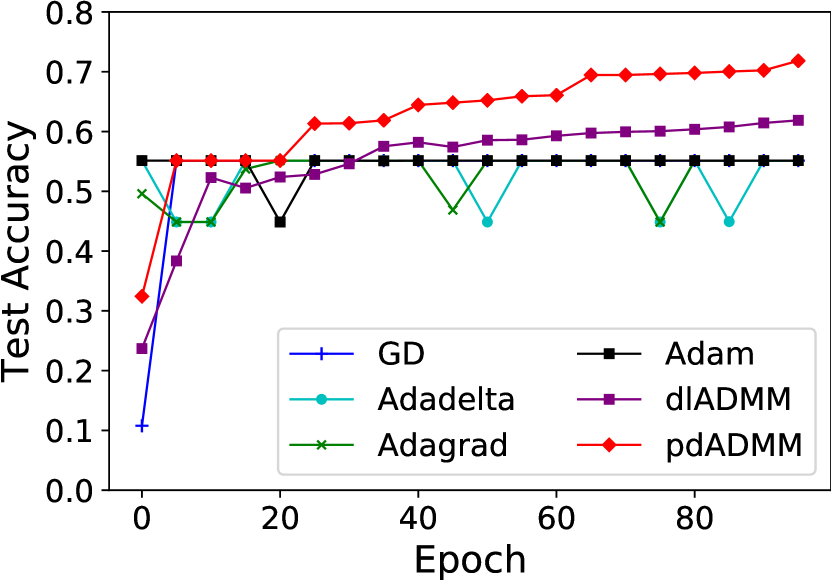
(d). SVHN

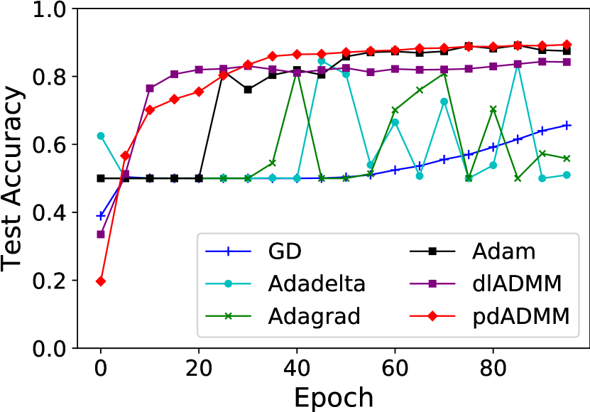
(e). CIFAR10

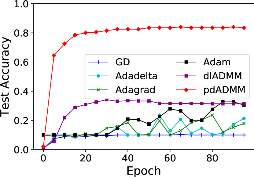
(f). CIFAR100

Figure 6: Test Accuracy of all methods: pdADMM outperformed most comparison methods.

V-D1 Experimental Settings

In order to evaluate accuracy, we used the same architecture as the previous section. $\nu$ and $\rho$ were set to $10^{-4}$ in order to maximize the performance of training data. The number of epoch was set to $100$. In this experiment, the full batch was used for training. As suggested by the training strategy in Section III-B, we firstly trained a feed-forward neural network with five hidden layers, and then all layers were involved in training.

V-D2 Comparison Methods

SGD and its variants are state-of-the-art methods and hence were served as comparison methods. For SGD-based methods, the full batch dataset is used for training models. All parameters were chosen by maximizing the accuracy of training datasets. The baselines are described as follows:
1. Gradient Descent (GD) [49]. The GD and its variants are the most popular deep learning optimizers, whose convergence has been studied extensively in the literature. The learning rate of GD was set to $0.01$.
2. Adaptive learning rate method (Adadelta) [50]. The Adadelta is proposed to overcome the sensitivity to hyperparameter selection. The learning rate of Adadelta was set to $1$.
3. Adaptive gradient algorithm (Adagrad) [51]. Adagrad is an improved version of SGD: rather than fixing the learning rate during training, it adapts the learning rate to the hyperparameter. The learning rate of Adagrad was set to $0.1$.
4. Adaptive momentum estimation (Adam) [52]. Adam is the most popular optimization method for deep learning models. It estimates the first and second momentum to correct the biased gradient and thus makes convergence fast. The learning rate of Adam was set to $0.001$.
5. Deep learning Alternaing Direction Method of Multipliers (dlADMM) [2]. The dlADMM is an improvement of the previous ADMM implementation [1]. It is guaranteed to converge to a critical point with a rate of $o(1/k)$. $\rho$ and $\nu$ were both set to $10^{-6}$.

V-D3 Performance

In this section, the performance of the proposed pdADMM is analyzed against comparison methods. Figures 5 and 6 show the training and test accuracy of the proposed pdADMM against comparison methods on six datasets, respectively. X-axis and Y-axis represent epoch and training accuracy, respectively. Overall, the pdADMM outperformed most of comparison methods: it performed the best on the SVHN, CIFAR10 and CIFAR100 datasets, while was only secondary to Adam on the MNIST, Fashion MNIST and kMNIST datasets. The performance gap is particularly obvious on the CIFAR100 dataset. Most SGD-type methods suffered from gradient vanishing in the deep neural network, and struggled to find an optimum: for example, GD can only reach $10\%$ training accuracy on the MNIST dataset; Adagrad and Adadelta performed better then GD, but took many epochs to escape saddle points. The dlADMM can avoid gradient vanishing problem, however, it performed worse than the proposed pdADMM on all datasets. Adam performed the best on three MNIST-like datasets, but performed worse than the proposed pdADMM on three other datasets, which are hard to train with high accuracy than three MNIST-like datasets. This indicates that the proposed pdADMM may be more suitable for training hard datasets than Adam.

VI Conclusion

Alternating Direction Method of Multipliers (ADMM) is considered to be a good alternative to Stochastic gradient descent (SGD) for training deep neural networks. In this paper, we propose a novel parallel deep learning Alternating Direction Method of Multipliers (pdADMM) to achieve layer parallelism. The proposed pdADMM is guaranteed to converge to a critical solution under mild conditions. Experiments on benchmark datasets demonstrate that our proposed pdADMM can lead to a huge speedup when training a deep feed-forward neural network, it also outperformed others on six benchmark datasets.

Proof of Theorem 3

Proof.

To prove this theorem, we will first show that $c_{k}$ satisfies two conditions: (1). $c_{k}\geq c_{k+1}$. (2). $\sum\nolimits_{k=0}^{\infty}c_{k}$ is bounded. Specifically, first, we have

$$c_{k} \!=\!\min\nolimits_{0\leq i\leq k}\!(\sum\nolimits_{l=2}^{L}(\tau^{i+1}_{l}/2)\|p^{i+1}_{l}\!-\!p^{i}_{l}\|^{2}_{2}$$

$$+\sum\nolimits_{l\!=\!1}^{L}(\theta^{i\!+\!1}_{l}/2)\|W^{i\!+\!1}_{l}\!-\!W^{i}_{l}\|^{2}_{2}+\sum\nolimits_{l\!=\!1}^{L}(\nu/2)\|b^{i\!+\!1}_{l}\!-\!b^{i}_{l}\|^{2}_{2}$$

$$+\sum\nolimits_{l=1}^{L-1}C_{1}\|z^{i+1}_{l}-z^{i}_{l}\|^{2}_{2}+(\nu/2)\|z^{i+1}_{L}-z^{i}_{L}\|^{2}_{2}$$

$$+\sum\nolimits_{l=1}^{L-1}C_{2}\|q^{i+1}_{l}-q^{i}_{l}\|^{2}_{2})$$

$$\geq\!\min\nolimits_{0\leq i\leq k+1}\!(\sum\nolimits_{l=2}^{L}(\tau^{i+1}_{l}/2)\|p^{i+1}_{l}\!-\!p^{i}_{l}\|^{2}_{2}$$

$$+\sum\nolimits_{l\!=\!1}^{L}(\theta^{i\!+\!1}_{l}/2)\|W^{i\!+\!1}_{l}\!-\!W^{i}_{l}\|^{2}_{2}+\sum\nolimits_{l\!=\!1}^{L}(\nu/2)\|b^{i\!+\!1}_{l}\!-\!b^{i}_{l}\|^{2}_{2}$$

$$+\sum\nolimits_{l=1}^{L-1}C_{1}\|z^{i+1}_{l}-z^{i}_{l}\|^{2}_{2}+(\nu/2)\|z^{i+1}_{L}-z^{i}_{L}\|^{2}_{2}$$

$$+\sum\nolimits_{l=1}^{L-1}C_{2}\|q^{i+1}_{l}-q^{i}_{l}\|^{2}_{2})$$

$$=c_{k+1}$$

Therefore $c_{k}$ satisfies the first condition. Second,

$$\sum\nolimits_{k\!=\!0}^{\infty}c_{k}=\sum\nolimits_{k=0}^{\infty}\min\nolimits_{0\leq i\leq k}\!(\sum\nolimits_{l=2}^{L}(\tau^{i+1}_{l}/2)\|p^{i+1}_{l}\!-\!p^{i}_{l}\|^{2}_{2}$$

$$+\sum\nolimits_{l\!=\!1}^{L}(\theta^{i\!+\!1}_{l}/2)\|W^{i\!+\!1}_{l}\!-\!W^{i}_{l}\|^{2}_{2}+\sum\nolimits_{l\!=\!1}^{L}(\nu/2)\|b^{i\!+\!1}_{l}\!-\!b^{i}_{l}\|^{2}_{2}$$

$$+\sum\nolimits_{l=1}^{L-1}C_{1}\|z^{i+1}_{l}-z^{i}_{l}\|^{2}_{2}+(\nu/2)\|z^{i+1}_{L}-z^{i}_{L}\|^{2}_{2}$$

$$+\sum\nolimits_{l=1}^{L-1}C_{2}\|q^{i+1}_{l}-q^{i}_{l}\|^{2}_{2})$$

$$\leq\sum\nolimits_{k=0}^{\infty}(\sum\nolimits_{l=2}^{L}(\tau^{k+1}_{l}/2)\|p^{k+1}_{l}\!-\!p^{k}_{l}\|^{2}_{2}$$

$$+\sum\nolimits_{l\!=\!1}^{L}(\theta^{k\!+\!1}_{l}/2)\|W^{k\!+\!1}_{l}\!-\!W^{k}_{l}\|^{2}_{2}+\sum\nolimits_{l\!=\!1}^{L}(\nu/2)\|b^{k\!+\!1}_{l}\!-\!b^{k}_{l}\|^{2}_{2}$$

$$+\sum\nolimits_{l=1}^{L-1}C_{1}\|z^{k+1}_{l}-z^{k}_{l}\|^{2}_{2}+(\nu/2)\|z^{k+1}_{L}-z^{k}_{L}\|^{2}_{2}$$

$$+\sum\nolimits_{l=1}^{L-1}C_{2}\|q^{k+1}_{l}-q^{k}_{l}\|^{2}_{2})$$

$$\leq L_{\rho}(\textbf{p}^{0},\textbf{W}^{0},\textbf{b}^{0},\textbf{z}^{0},\textbf{q}^{0},\textbf{u}^{0})-L_{\rho}(\textbf{p}^{*},\textbf{W}^{*},\textbf{b}^{*},\textbf{z}^{*},\textbf{q}^{*},\textbf{u}^{*})$$

(Lemma 1)

So $c_{k}$ satisfies the second condition. Finally, since we have proved the first two conditions and the third one $c_{k}\geq 0$ is obvious, the convergence rate of $o(1/k)$ is proven (Lemma 1.2 in [53]). ∎

Preliminary Results

Lemma 4.

It holds for every $k\in\mathbb{N}$ and $l=1,\cdots,L-1$ that

$$u^{k}_{l}=\nu(q^{k}_{l}-f_{l}(z^{k}_{l}))$$

Proof.

This follows directly from the optimality condition of $q^{k}_{l}$ and Equation (7). ∎

Lemma 5.

It holds for every $k\in\mathbb{N}$ and $l=1,\cdots,L-1$ that

$$\|u^{k+1}_{l}-u^{k}_{l}\|\leq\nu\|q^{k+1}_{l}-q^{k}_{l}\|+\nu S\|z^{k+1}_{l}-z^{k}_{l}\|$$

Proof.

$$\|u^{k+1}_{l}-u^{k}_{l}\|$$

$$=\|\nu(q^{k+1}_{l}-f_{l}(z^{k+1}_{l}))-\nu(q^{k}_{l}-f_{l}(z^{k}_{l}))\|\text{(Lemma \ref{lemma: q_opt})}$$

$$\leq\nu\|q^{k+1}_{l}-q^{k}_{l}\|+\nu\|f_{l}(z^{k+1}_{l})-f_{l}(z^{k}_{l})\|\text{(triangle inequality)}$$

$$\leq\nu\|q^{k+1}_{l}-q^{k}_{l}\|+\nu S\|z^{k+1}_{l}-z^{k}_{l}\|\text{(Assumption \ref{ass:lipschitz continuous})}$$

∎

Lemma 6.

It holds for every $k\in\mathbb{N}$ and $l=1,\cdots,L-1$ that

$$\|u^{k+1}_{l}-u^{k}_{l}\|^{2}_{2}\leq 2\nu^{2}(\|q^{k+1}_{l}-q^{k}_{l}\|^{2}_{2}+S^{2}\|z^{k+1}_{l}-z^{k}_{l}\|^{2}_{2})$$

Proof.

$$\|u^{k+1}_{l}-u^{k}_{l}\|^{2}_{2} =\nu^{2}\|q^{k+1}_{l}-f_{l}(z^{k+1}_{l})-q^{k}_{l}+f_{l}(z^{k}_{l})\|^{2}_{2}\text{(Lemma \ref{lemma: q_opt})}$$

$$\leq 2\nu^{2}(\|q^{k+1}_{l}-q^{k}_{l}\|^{2}_{2}+\|f_{l}(z^{k+1}_{l})-f_{l}(z^{k}_{l})\|^{2}_{2})\text{(mean inequality)}$$

$$\leq 2\nu^{2}(\|q^{k+1}_{l}-q^{k}_{l}\|^{2}_{2}+S^{2}\|z^{k+1}_{l}-z^{k}_{l}\|^{2}_{2})\text{(Assumption \ref{ass:lipschitz continuous})}$$

∎

Lemma 7.

For every $k\in\mathbb{N}$, it holds that

$$L_{\rho}(\textbf{p}^{k},\textbf{W}^{k},\textbf{b}^{k},\textbf{z}^{k},\textbf{q}^{k},\textbf{u}^{k})\!-\!L_{\rho}(\textbf{p}^{k+1},\textbf{W}^{k},\textbf{b}^{k},\textbf{z}^{k},\textbf{q}^{k},\textbf{u}^{k})\geq\sum\nolimits_{l=2}^{L}(\tau^{k+1}_{l}/2)\|p^{k+1}_{l}-p^{k}_{l}\|^{2}_{2}$$ (9)

$$L_{\rho}(\textbf{p}^{k\!+\!1},\textbf{W}^{k},\textbf{b}^{k},\textbf{z}^{k},\textbf{q}^{k},\textbf{u}^{k})\!-\!L_{\rho}(\textbf{p}^{k\!+\!1},\textbf{W}^{k\!+\!1},\textbf{b}^{k},\textbf{z}^{k},\textbf{q}^{k},\textbf{u}^{k})\!\geq\!\sum\nolimits_{l\!=\!1}^{L}(\theta^{k\!+\!1}_{l}/2)\|W^{k\!+\!1}_{l}\!-\!W^{k}_{l}\|^{2}_{2}$$ (10)

$$L_{\rho}(\textbf{p}^{k\!+\!1},\textbf{W}^{k\!+\!1},\textbf{b}^{k},\textbf{z}^{k},\textbf{q}^{k},\textbf{u}^{k})\!-\!L_{\rho}(\textbf{p}^{k\!+\!1},\textbf{W}^{k\!+\!1},\textbf{b}^{k\!+\!1},\textbf{z}^{k},\textbf{q}^{k},\textbf{u}^{k})\geq(\nu/2)\sum\nolimits_{l\!=\!1}^{L}\|b^{k\!+\!1}_{l}\!-\!b^{k}_{l}\|^{2}_{2}$$ (11)

$$L_{\rho}(\textbf{p}^{k\!+\!1},\textbf{W}^{k\!+\!1},\textbf{b}^{k\!+\!1},\textbf{z}^{k},\textbf{q}^{k},\textbf{u}^{k})\!-\!L_{\rho}(\textbf{p}^{k\!+\!1},\textbf{W}^{k\!+\!1},\textbf{b}^{k\!+\!1},\textbf{z}^{k\!+\!1},\textbf{q}^{k},\textbf{u}^{k})\geq(\nu/2)\sum\nolimits_{l\!=\!1}^{L}\|z^{k\!+\!1}_{l}\!-\!z^{k}_{l}\|^{2}_{2}$$ (12)

Proof.

Generally, all inequalities can be obtained by applying optimality conditions of updating p, W, b and z, respectively. We only prove Inequalities (9), (11) and (12).This is because Inequality (10) follows the same routine of Inequality (9).
Firstly, we focus on Inequality (9). The choice of $\tau^{k+1}_{l}$ requires

$$\phi(p^{k+1}_{l},W^{k}_{l},b^{k}_{l},z^{k}_{l},q^{k}_{l-1},u^{k}_{l-1})\leq U_{l}(p^{k+1}_{l};\tau^{k+1}_{l})$$ (13)

Moreover, the optimality condition of Equation (1) leads to

$$\nabla_{p^{k}_{l}}\phi(p^{k}_{l},W^{k}_{l},b^{k}_{l},z^{k}_{l},q^{k}_{l-1},u^{k}_{l-1})+\tau^{k+1}_{l}(p^{k+1}_{l}-p^{k}_{l})=0$$ (14)

Therefore

$$L_{\rho}(\textbf{p}^{k},\textbf{W}^{k},\textbf{b}^{k},\textbf{z}^{k},\textbf{q}^{k},\textbf{u}^{k})\!-\!L_{\rho}(\textbf{p}^{k+1},\textbf{W}^{k},\textbf{b}^{k},\textbf{z}^{k},\textbf{q}^{k},\textbf{u}^{k})$$

$$=\sum\nolimits_{l=2}^{L}(\phi(p^{k}_{l},W^{k}_{l},b^{k}_{l},z^{k}_{l},q^{k}_{l-1},u^{k}_{l-1})-\phi(p^{k+1}_{l},W^{k}_{l},b^{k}_{l},z^{k}_{l},q^{k}_{l-1},u^{k}_{l-1}))$$

$$\geq\sum\nolimits_{l=2}^{L}(\phi(p^{k}_{l},W^{k}_{l},b^{k}_{l},z^{k}_{l},q^{k}_{l-1},u^{k}_{l-1})-U_{l}(p^{k+1}_{l};\tau^{k+1}_{l}))\text{(Inequality \eqref{eq:stop condition})}$$

$$=\sum\nolimits_{l=2}^{L}(-\nabla_{p^{k}_{l}}\phi^{T}(p^{k}_{l},W^{k}_{l},b^{k}_{l},z^{k}_{l},q^{k}_{l-1},u^{k}_{l-1})(p^{k+1}_{l}-p^{k}_{l})-({\tau}^{k+1}_{l}/2)\|p^{k+1}_{l}-p^{k}_{l}\|^{2}_{2})$$

$$=\sum\nolimits_{l=2}^{L}(\tau^{k+1}_{l}/2)\|p^{k+1}_{l}-p^{k}_{l}\|^{2}_{2}\text{(Equation \eqref{eq:p optimality condition})}$$

Next, we prove Inequality (11). Because $\nabla_{{b}_{1}}\phi({p}_{1},{W}_{1},{b}_{1},{z}_{1})$ and $\nabla_{{b}_{l}}\phi({p}_{l},{W}_{l},{b}_{l},{z}_{l},{q}_{l},{u}_{l})$ are Lipschitz continuous with coefficient $\nu$. According to Lemma 2.1 in [41], we have

$$\phi({p}^{k\!+\!1}_{1},{W}^{k+1}_{1},{b}^{k+1}_{1},{z}^{k}_{1}) \leq\phi({p}^{k\!+\!1}_{1},{W}^{k+1}_{1},{b}^{k}_{1},{z}^{k}_{1})+\nabla_{{b}^{k}_{1}}\phi^{T}({p}^{k\!+\!1}_{1},{W}^{k+1}_{1},{b}^{k}_{1},{z}^{k}_{1})(b^{k+1}_{1}-b^{k}_{1})$$

$$+(\nu/2)\|b_{1}^{k+1}-b_{1}^{k}\|^{2}_{2}$$ (15)

$$\phi({p}^{k\!+\!1}_{l},{W}^{k+1}_{l},{b}^{k+1}_{l},{z}^{k}_{l},{q}^{k}_{l-1},{u}^{k}_{l-1}) \leq\phi({p}^{k\!+\!1}_{l},{W}^{k+1}_{l},{b}^{k}_{l},{z}^{k}_{l},{q}^{k}_{l-1},{u}^{k}_{l-1})$$

$$+\nabla_{{b}^{k}_{l}}\phi^{T}({p}^{k\!+\!1}_{l},{W}^{k+1}_{l},{b}^{k}_{l},{z}^{k}_{l},{q}^{k}_{l-1},{u}^{k}_{l-1})(b^{k+1}_{l}-b^{k}_{l})$$

$$+(\nu/2)\|b_{l}^{k+1}-b_{l}^{k}\|^{2}_{2}$$ (16)

Moreover, the optimality condition of Equation (3) leads to

$$\nabla_{b^{k}_{1}}\phi(p^{k}_{1},W^{k}_{1},b^{k}_{1},z^{k}_{1})+\nu(b^{k+1}_{1}-b^{k}_{1})=0$$ (17)

$$\nabla_{b^{k}_{l}}\phi(p^{k}_{l},W^{k}_{l},b^{k}_{l},z^{k}_{l},q^{k}_{l-1},u^{k}_{l-1})+\nu(b^{k+1}_{l}-b^{k}_{l})=0$$ (18)

Therefore, we have

$$L_{\rho}(\textbf{p}^{k\!+\!1},\textbf{W}^{k+1},\textbf{b}^{k},\textbf{z}^{k},\textbf{q}^{k},\textbf{u}^{k})\!-\!L_{\rho}(\textbf{p}^{k\!+\!1},\textbf{W}^{k\!+\!1},\textbf{b}^{k+1},\textbf{z}^{k},\textbf{q}^{k},\textbf{u}^{k})$$

$$=\phi({p}^{k\!+\!1}_{1},{W}^{k+1}_{1},{b}^{k}_{1},{z}^{k}_{1})-\phi({p}^{k\!+\!1}_{1},{W}^{k+1}_{1},{b}^{k+1}_{1},{z}^{k}_{1})$$

$$+\sum\nolimits_{l=2}^{L}(\phi({p}^{k\!+\!1}_{l},{W}^{k+1}_{l},{b}^{k}_{l},{z}^{k}_{l},q^{k}_{l-1},u^{k}_{l-1})-\phi({p}^{k\!+\!1}_{l},{W}^{k+1}_{l},{b}^{k+1}_{l},{z}^{k}_{l},q^{k}_{l-1},u^{k}_{l-1}))$$

$$\geq-\nabla_{{b}^{k}_{1}}\phi^{T}({p}^{k\!+\!1}_{1},{W}^{k+1}_{1},{b}^{k}_{1},{z}^{k}_{1})(b^{k+1}_{1}-b^{k}_{1})-(\nu/2)\|b_{1}^{k+1}-b_{1}^{k}\|^{2}_{2}$$

$$+\sum\nolimits_{l=2}^{L}(-\nabla_{{b}^{k}_{l}}\phi^{T}({p}^{k\!+\!1}_{l},{W}^{k+1}_{l},{b}^{k}_{l},{z}^{k}_{l},{q}^{k}_{l-1},{u}^{k}_{l-1})(b^{k+1}_{l}-b^{k}_{l})-(\nu/2)\|b_{l}^{k+1}-b_{l}^{k}\|^{2}_{2})$$

(Inequalities (15) and (16))

$$=(\nu/2)\sum\nolimits_{l=1}^{L}\|b^{k+1}_{l}-b^{k}_{l}\|^{2}_{2}\text{(Equations \eqref{eq:b1 optimality condition} and \eqref{eq:b optimality condition})}$$

Finally, we prove Inequality (12). Because $z^{k+1}_{l}$ minimizes Equation (4), we have

$$(\nu/2)\|z^{k+1}_{l}-W^{k+1}_{l}p^{k+1}_{l}-b^{k+1}_{l}\|^{2}_{2}+(\nu/2)\|q^{k}_{l}-f_{l}(z^{k+1}_{l})\|^{2}_{2}+(\nu/2)\|z^{k+1}_{l}-z^{k}_{l}\|^{2}_{2}$$

$$\leq(\nu/2)\|z^{k}_{l}-W^{k+1}_{l}p^{k+1}_{l}-b^{k+1}_{l}\|^{2}_{2}+(\nu/2)\|q^{k}_{l}-f_{l}(z^{k}_{l})\|^{2}_{2}$$ (19)

And

$$R(z^{k}_{L};y)\!+(\nu/2)\!\|z^{k}_{L}\!-\!W^{k\!+\!1}_{L}p^{k\!+\!1}_{L}\!-\!b^{k\!+\!1}_{L}\|^{2}_{2}-R(z^{k+1}_{L};y)\!-(\nu/2)\!\|z^{k+1}_{L}\!-\!W^{k\!+\!1}_{L}p^{k\!+\!1}_{L}\!-\!b^{k\!+\!1}_{L}\|^{2}_{2}$$

$$=R(z^{k}_{L};y)-R(z^{k+1}_{L};y)+(\nu/2)\|z^{k}_{L}-z^{k+1}_{L}\|^{2}_{2}+\nu(z^{k+1}_{L}-W^{k+1}_{L}p^{k+1}_{L}-b^{k+1}_{L})^{T}(z^{k}_{L}-z_{L}^{k+1})$$

($$\|a-b\|^{2}_{2}-\|a-c\|^{2}_{2}=\|b-c\|^{2}_{2}+2(c-a)^{T}(b-c) a=W^{k+1}_{L}p^{k+1}_{L}+b^{k+1}_{L} b=z^{k}_{L} c=z^{k+1}_{L}$$ where , , and )

$$\geq s^{T}(z^{k}_{L}-z^{k+1}_{L})+(\nu/2)\|z^{k}_{L}-z^{k+1}_{L}\|^{2}_{2}+\nu(z^{k+1}_{L}-W^{k+1}_{L}p^{k+1}_{L}-b^{k+1}_{L})^{T}(z^{k}_{L}-z_{L}^{k+1})$$

($$s\in\partial R(z^{k+1}_{L};y) R(z^{k+1}_{L};y)$$ is a subgradient of )

$$=(\nu/2)\|z^{k+1}_{L}-z^{k}_{L}\|^{2}_{2}$$ (20)

($$0\in s+\nu(z^{k+1}_{L}-W^{k+1}_{L}p^{k+1}_{L}-b^{k+1}_{L})$$ by the optimality condition of Equation (5))

Therefore

$$L_{\rho}(\textbf{p}^{k\!+\!1},\textbf{W}^{k\!+\!1},\textbf{b}^{k\!+\!1},\textbf{z}^{k},\textbf{q}^{k},\textbf{u}^{k})\!-\!L_{\rho}(\textbf{p}^{k\!+\!1},\textbf{W}^{k\!+\!1},\textbf{b}^{k\!+\!1},\textbf{z}^{k\!+\!1},\textbf{q}^{k},\textbf{u}^{k})$$

$$=\sum\nolimits_{i=1}^{L-1}((\nu/2)\|z^{k}_{l}-W^{k+1}_{l}p^{k+1}_{l}-b^{k+1}_{l}\|^{2}_{2}+(\nu/2)\|q^{k}_{l}-f_{l}(z^{k}_{l})\|^{2}_{2}$$

$$-(\nu/2)\|z^{k+1}_{l}-W^{k+1}_{l}p^{k+1}_{l}-b^{k+1}_{l}\|^{2}_{2}-(\nu/2)\|q^{k}_{l}-f_{l}(z^{k+1}_{l})\|^{2}_{2})$$

$$+R(z^{k}_{L};y)\!+(\nu/2)\!\|z^{k}_{L}\!-\!W^{k\!+\!1}_{L}p^{k\!+\!1}_{L}\!-\!b^{k\!+\!1}_{L}\|^{2}_{2}-R(z^{k+1}_{L};y)\!-(\nu/2)\!\|z^{k+1}_{L}\!-\!W^{k\!+\!1}_{L}p^{k\!+\!1}_{L}\!-\!b^{k\!+\!1}_{L}\|^{2}_{2}$$

$$\geq(\nu/2)\sum\nolimits_{l=1}^{L}\|z^{k+1}_{l}-z^{k}_{l}\|^{2}_{2}\text{(Inequalities \eqref{eq:z minimize} and \eqref{eq:zl minimize})}$$

∎

Lemma 8.

For every $k\in N$, it holds that

$$L_{\rho}(\textbf{p}^{k\!+\!1},\textbf{W}^{k\!+\!1},\textbf{b}^{k\!+\!1},\textbf{z}^{k+1},\textbf{q}^{k},\textbf{u}^{k})\!-\!L_{\rho}(\textbf{p}^{k\!+\!1},\textbf{W}^{k\!+\!1},\textbf{b}^{k\!+\!1},\textbf{z}^{k\!+\!1},\textbf{q}^{k+1},\textbf{u}^{k+1})$$

$$\geq\sum\nolimits_{l=1}^{L-1}((\rho/2-2\nu^{2}/\rho-\nu/2)\|q^{k+1}_{l}-q^{k}_{l}\|^{2}_{2}-(2\nu^{2}S^{2}/\rho)\|z^{k+1}_{l}-z^{k}_{l}\|^{2}_{2})$$ (21)

Proof.

$$L_{\rho}(\textbf{p}^{k\!+\!1},\textbf{W}^{k\!+\!1},\textbf{b}^{k\!+\!1},\textbf{z}^{k+1},\textbf{q}^{k},\textbf{u}^{k})\!-\!L_{\rho}(\textbf{p}^{k\!+\!1},\textbf{W}^{k\!+\!1},\textbf{b}^{k\!+\!1},\textbf{z}^{k\!+\!1},\textbf{q}^{k+1},\textbf{u}^{k+1})$$

$$=\sum\nolimits_{l=1}^{L-1}((\nu/2)\|f_{l}(z^{k+1}_{l})-q^{k}_{l}\|^{2}_{2}-(\nu/2)\|f_{l}(z^{k+1}_{l})-q^{k+1}_{l}\|^{2}_{2}-(u^{k+1}_{l})^{T}(q^{k}_{l}-q^{k+1}_{l})$$

$$+(\rho/2)\|q^{k+1}_{l}-q^{k}_{l}\|^{2}_{2}-(1/\rho)\|u^{k+1}_{l}-u^{k}_{l}\|^{2}_{2})$$

$$=\sum\nolimits_{l=1}^{L-1}((\nu/2)\|f_{l}(z^{k+1}_{l})-q^{k}_{l}\|^{2}_{2}-(\nu/2)\|f_{l}(z^{k+1}_{l})-q^{k+1}_{l}\|^{2}_{2}-\nu(q^{k+1}_{l}-f_{l}(z^{k+1}_{l}))^{T}(q^{k}_{l}-q^{k+1}_{l})$$

$$+(\rho/2)\|q^{k+1}_{l}-q^{k}_{l}\|^{2}_{2}-(1/\rho)\|u^{k+1}_{l}-u^{k}_{l}\|^{2}_{2})\text{(Lemma \ref{lemma: q_opt})}$$

$$\geq\sum\nolimits_{l=1}^{L-1}(-(\nu/2)\|q^{k+1}_{l}-q^{k}_{l}\|^{2}_{2}+(\rho/2)\|q^{k+1}_{l}-q^{k}_{l}\|^{2}_{2}-(1/\rho)\|u^{k+1}_{l}-u^{k}_{l}\|^{2}_{2})$$

($$-\nu(q_{l}-f_{l}(z^{k+1}_{l}))=-(\nu/2)\nabla_{q_{l}}\|q_{l}-f_{l}(z^{k+1}_{l})\|^{2}_{2} q_{l}$$ is lipschitz continuous with regard to and Lemma 2.1 in [41])

$$\geq\sum\nolimits_{l=1}^{L-1}(-(\nu/2)\|q^{k+1}_{l}-q^{k}_{l}\|^{2}_{2}+(\rho/2)\|q^{k+1}_{l}-q^{k}_{l}\|^{2}_{2}-(2\nu^{2}/\rho)\|q^{k+1}_{l}-q^{k}_{l}\|^{2}_{2}-(2\nu^{2}S^{2}/\rho)\|z^{k+1}_{l}-z^{k}_{l}\|^{2}_{2})$$

(Lemma 6)

$$=\sum\nolimits_{l=1}^{L-1}((\rho/2-2\nu^{2}/\rho-\nu/2)\|q^{k+1}_{l}-q^{k}_{l}\|^{2}_{2}-(2\nu^{2}S^{2}/\rho)\|z^{k+1}_{l}-z^{k}_{l}\|^{2}_{2})$$

∎

Proof of Lemma 1

Proof.

We sum up Inequalities (9), (10), (11), (12), and (21) to obtain Inequality (8). ∎

Proof of Lemma 2

Proof.

There exists $\textbf{q}^{{}^{\prime}}$ such that $p^{k}_{l+1}=q^{{}^{\prime}}_{l}$ and

$$F(\textbf{p}^{k},\textbf{W}^{k},\textbf{b}^{k},\textbf{z}^{k},\textbf{q}^{{}^{\prime}})\geq\min\nolimits_{\textbf{p},\textbf{W},\textbf{b},\textbf{z},\textbf{q}}\{F(\textbf{p},\textbf{W},\textbf{b},\textbf{z},\textbf{q})|p_{l+1}=q_{l}\}>-\infty$$

Therefore, we have

$$L_{\rho}(\textbf{p}^{k},\textbf{W}^{k},\textbf{b}^{k},\textbf{z}^{k},\textbf{q}^{k},\textbf{u}^{k})=F(\textbf{p}^{k},\textbf{W}^{k},\textbf{b}^{k},\textbf{z}^{k},\textbf{q}^{k})+\sum\nolimits_{l=1}^{L}(u^{k}_{l})^{T}(p^{k}_{l+1}-q^{k}_{l})+(\rho/2)\|p^{k}_{l+1}-q^{k}_{l}\|^{2}_{2}$$

$$=R(z^{k}_{L};y)+(\nu/2)(\sum\nolimits_{l=1}^{L}\|z^{k}_{l}-W^{k}_{l}p^{k}_{l}-b^{k}_{l}\|^{2}_{2}+\sum\nolimits_{l=1}^{L-1}\|q^{k}_{l}-f_{l}(z^{k}_{l})\|^{2}_{2})$$

$$+\sum\nolimits_{l=1}^{L-1}((u^{k}_{l})^{T}(p^{k}_{l+1}-q^{k}_{l})+(\rho/2)\|p^{k}_{l+1}-q^{k}_{l}\|^{2}_{2})$$

$$=R(z^{k}_{L};y)+(\nu/2)(\sum\nolimits_{l=1}^{L}\|z^{k}_{l}-W^{k}_{l}p^{k}_{l}-b^{k}_{l}\|^{2}_{2}+\sum\nolimits_{l=1}^{L-1}\|q^{k}_{l}-f_{l}(z^{k}_{l})\|^{2}_{2})$$

$$+\sum\nolimits_{l=1}^{L-1}(\nu(q^{k}_{l}-f_{l}(z^{k}_{l}))^{T}(q^{{}^{\prime}}_{l}-q^{k}_{l})+(\rho/2)\|p^{k}_{l+1}-q^{k}_{l}\|^{2}_{2})$$

($$p^{k}_{l+1}=q^{{}^{\prime}}_{l}$$ and Lemma 4)

$$\geq R(z^{k}_{L};y)+(\nu/2)(\sum\nolimits_{l=1}^{L}\|z^{k}_{l}-W^{k}_{l}p^{k}_{l}-b^{k}_{l}\|^{2}_{2}+\sum\nolimits_{l=1}^{L-1}\|q^{{}^{\prime}}_{l}-f_{l}(z^{k}_{l})\|^{2}_{2})$$

$$-\sum\nolimits_{l=1}^{L-1}(\nu/2)\|q^{{}^{\prime}}_{l}-q^{k}_{l}\|^{2}_{2}+\sum\nolimits_{l=1}^{L-1}(\rho/2)\|p^{k}_{l+1}-q^{k}_{l}\|^{2}_{2})$$

($$\nu(q_{l}-f_{l}(z^{k+1}_{l}))=(\nu/2)\nabla_{q_{l}}\|q_{l}-f_{l}(z^{k+1}_{l})\|^{2}_{2} q_{l}$$ is lipschitz continuous with regard to and Lemma 2.1 in [41])

$$=F(\textbf{p}^{k},\textbf{W}^{k},\textbf{b}^{k},\textbf{z}^{k},\textbf{q}^{{}^{\prime}})+(\rho-\nu)/2\|p^{k}_{l+1}-q^{k}_{l}\|^{2}_{2}>-\infty$$

Therefore, $F(\textbf{p}^{k},\textbf{W}^{k},\textbf{b}^{k},\textbf{z}^{k},\textbf{q}^{{}^{\prime}})$ and $(\rho-\nu)/2\|p^{k}_{l+1}-q^{k}_{l}\|^{2}_{2}$ are upper bounded by $L_{\rho}(\textbf{p}^{k},\textbf{W}^{k},\textbf{b}^{k},\textbf{z}^{k},\textbf{q}^{k},\textbf{u}^{k})$ and hence $L_{\rho}(\textbf{p}^{0},\textbf{W}^{0},\textbf{b}^{0},\textbf{z}^{0},\textbf{q}^{0},\textbf{u}^{0})$ (Lemma 1). From Assumption 1, $(\textbf{p}^{k},\textbf{W}^{k},\textbf{b}^{k},\textbf{z}^{k})$ is bounded. $\textbf{q}^{k}$ is also bounded because $(\rho-\nu)/2\|p^{k}_{l+1}-q^{k}_{l}\|^{2}_{2}$ is upper bounded. $\textbf{u}^{k}$ is bounded because of Lemma 4. ∎

Proof of Lemma 3

Proof.

We know that $\partial L_{\rho}(\textbf{p}^{k+1},\textbf{W}^{k+1},\textbf{b}^{k+1},\textbf{z}^{k+1},\textbf{q}^{k+1},\textbf{u}^{k+1})=\{\nabla_{\text{p}^{k+1}}L_{\rho},\nabla_{\text{W}^{k+1}}L_{\rho},\nabla_{\text{b}^{k+1}}L_{\rho},\partial_{\text{z}^{k+1}}L_{\rho},\nabla_{\text{q}^{k+1}}L_{\rho},\nabla_{\text{u}^{k+1}}L_{\rho}\}$ [2]. Specifically, we prove that $\|g\|$ is upper bounded by the linear combination of $\|\textbf{p}^{k+1}-\textbf{p}^{k}\|$,$\|\textbf{W}^{k+1}-\textbf{W}^{k}\|$, $\|\textbf{b}^{k+1}-\textbf{b}^{k}\|$, $\|\textbf{z}^{k+1}-\textbf{z}^{k}\|$, $\|\textbf{q}^{k+1}-\textbf{q}^{k}\|$, and $\|\textbf{u}^{k+1}-\textbf{u}^{k}\|$.
For $p^{k+1}_{l}$,

$$\nabla_{p^{k+1}_{l}}L_{\rho}(\textbf{p}^{k+1},\textbf{W}^{k+1},\textbf{b}^{k+1},\textbf{z}^{k+1},\textbf{q}^{k+1},\textbf{u}^{k+1})$$

$$=\nabla_{p^{k+1}_{l}}\phi({p}^{k+1}_{l},{W}^{k+1}_{l},{b}^{k+1}_{l},{z}^{k+1}_{l},q^{k+1}_{l-1},u^{k+1}_{l-1})$$

$$=\nabla_{p^{k}_{l}}\phi({p}^{k}_{l},{W}^{k}_{l},{b}^{k}_{l},{z}^{k}_{l},q^{k}_{l-1},u^{k}_{l-1})+\tau^{k+1}_{l}(p^{k+1}_{l}-p^{k}_{l})-\tau^{k+1}_{l}(p^{k+1}_{l}-p^{k}_{l})$$

$$+\nu(W^{k+1}_{l})^{T}W^{k+1}_{l}p^{k+1}_{l}-\nu(W^{k}_{l})^{T}W^{k}_{l}p^{k}_{l}+\nu(W^{k+1}_{l})^{T}b^{k+1}_{l}-\nu(W^{k}_{l})^{T}b^{k}_{l}-\nu(W^{k+1}_{l})^{T}z^{k+1}_{l}+\nu(W^{k}_{l})^{T}z^{k}_{l}$$

$$+(u^{k+1}_{l-1}-u^{k}_{l-1})+\rho(p^{k+1}_{l}-p^{k}_{l})-\rho(q^{k+1}_{l-1}-q^{k}_{l-1})$$

$$=-\tau^{k+1}_{l}(p^{k+1}_{l}-p^{k}_{l})+\nu(W^{k+1}_{l})^{T}W^{k+1}_{l}p^{k+1}_{l}-\nu(W^{k}_{l})^{T}W^{k}_{l}p^{k}_{l}+\nu(W^{k+1}_{l})^{T}b^{k+1}_{l}-\nu(W^{k}_{l})^{T}b^{k}_{l}$$

$$-\nu(W^{k+1}_{l})^{T}z^{k+1}_{l}+\nu(W^{k}_{l})^{T}z^{k}_{l}+(u^{k+1}_{l-1}-u^{k}_{l-1})+\rho(p^{k+1}_{l}-p^{k}_{l})-\rho(q^{k+1}_{l-1}-q^{k}_{l-1})$$

So

$$\|\nabla_{p^{k+1}_{l}}L_{\rho}(\textbf{p}^{k+1},\textbf{W}^{k+1},\textbf{b}^{k+1},\textbf{z}^{k+1},\textbf{q}^{k+1},\textbf{u}^{k+1})\|$$

$$=\|\tau^{k+1}_{l}(p^{k+1}_{l}-p^{k}_{l})+\nu(W^{k+1}_{l})^{T}W^{k+1}_{l}p^{k+1}_{l}-\nu(W^{k}_{l})^{T}W^{k}_{l}p^{k}_{l}+\nu(W^{k+1}_{l})^{T}b^{k+1}_{l}-\nu(W^{k}_{l})^{T}b^{k}_{l}$$

$$-\nu(W^{k+1}_{l})^{T}z^{k+1}_{l}+\nu(W^{k}_{l})^{T}z^{k}_{l}+(u^{k+1}_{l-1}-u^{k}_{l-1})+\rho(p^{k+1}_{l}-p^{k}_{l})-\rho(q^{k+1}_{l-1}-q^{k}_{l-1})\|$$

$$\leq\tau^{k+1}_{l}\|p^{k+1}_{l}-p^{k}_{l}\|+\nu\|(W^{k+1}_{l})^{T}W^{k+1}_{l}p^{k+1}_{l}-(W^{k}_{l})^{T}W^{k}_{l}p^{k}_{l}\|+\nu\|(W^{k+1}_{l})^{T}b^{k+1}_{l}-(W^{k}_{l})^{T}b^{k}_{l}\|$$

$$+\nu\|(W^{k+1}_{l})^{T}z^{k+1}_{l}-(W^{k}_{l})^{T}z^{k}_{l}\|+\|u^{k+1}_{l-1}-u^{k}_{l-1}\|+\rho\|p^{k+1}_{l}-p^{k}_{l}\|+\rho\|q^{k+1}_{l-1}-q^{k}_{l-1}\|\ \text{(triangle inequality)}$$

$$=\tau^{k+1}_{l}\|p^{k+1}_{l}-p^{k}_{l}\|+\nu\|(W^{k+1}_{l})^{T}W^{k+1}_{l}(p^{k+1}_{l}-p^{k}_{l})+(W^{k+1}_{l})^{T}(W^{k+1}_{l}-W^{k}_{l})p^{k}_{l}+(W^{k+1}_{l}-W^{k}_{l})^{T}W^{k}_{l}p^{k}_{l}\|$$

$$+\nu\|(W^{k+1}_{l})^{T}(b^{k+1}_{l}-b^{k}_{l})+(W^{k+1}_{l}-W^{k}_{l})^{T}b^{k}_{l}\|+\nu\|(W^{k+1}_{l})^{T}(z^{k+1}_{l}-z^{k}_{l})+(W^{k+1}_{l}-W^{k}_{l})^{T}z^{k}_{l}\|$$

$$+\|u^{k+1}_{l-1}-u^{k}_{l-1}\|+\rho\|p^{k+1}_{l}-p^{k}_{l}\|+\rho\|q^{k+1}_{l-1}-q^{k}_{l-1}\|$$

$$\leq\tau^{k+1}_{l}\|p^{k+1}_{l}-p^{k}_{l}\|+\nu\|W^{k+1}_{l}\|^{2}\|p^{k+1}_{l}-p^{k}_{l}\|+\nu\|W^{k+1}_{l}\|\|W^{k+1}_{l}-W^{k}_{l}\|\|p^{k}_{l}\|+\nu\|W^{k+1}_{l}-W^{k}_{l}\|\|W^{k}_{l}\|\|p^{k}_{l}\|$$

$$+\nu\|W^{k+1}_{l}\|\|b^{k+1}_{l}-b^{k}_{l}\|+\nu\|W^{k+1}_{l}-W^{k}_{l}\|\|b^{k}_{l}\|+\nu\|W^{k+1}_{l}\|\|z^{k+1}_{l}-z^{k}_{l}\|+\nu\|W^{k+1}_{l}-W^{k}_{l}\|\|z^{k}_{l}\|$$

$$+\nu(\|q^{k+1}_{l-1}-q^{k}_{l-1}\|+S\|z^{k+1}_{l-1}-z^{k}_{l-1}\|)+\rho\|p^{k+1}_{l}-p^{k}_{l}\|+\rho\|q^{k+1}_{l-1}-q^{k}_{l-1}\|$$

(triangle inequality, Cauthy-Schwartz inequality and Lemma 5)

$$\leq\tau^{k+1}_{l}\|p^{k+1}_{l}-p^{k}_{l}\|+\nu\mathbb{N}^{2}_{\textbf{W}}\|p^{k+1}_{l}-p^{k}_{l}\|+2\nu\mathbb{N}_{\textbf{W}}\mathbb{N}_{\textbf{p}}\|W^{k+1}_{l}-W^{k}_{l}\|+\nu\mathbb{N}_{\textbf{W}}\|b^{k+1}_{l}-b^{k}_{l}\|+\nu\mathbb{N}_{\textbf{b}}\|W^{k+1}_{l}-W^{k}_{l}\|$$

$$+\nu\mathbb{N}_{\textbf{W}}\|z^{k+1}_{l}-z^{k}_{l}\|+\nu\mathbb{N}_{\textbf{z}}\|W^{k+1}_{l}-W^{k}_{l}\|+2\nu^{2}(\|q^{k+1}_{l-1}-q^{k}_{l-1}\|^{2}_{2}+S^{2}\|z^{k+1}_{l-1}-z^{k}_{l-1}\|^{2}_{2})+\rho\|p^{k+1}_{l}-p^{k}_{l}\|+\rho\|q^{k+1}_{l-1}-q^{k}_{l-1}\|$$

(Lemma 2)

For $W^{k+1}_{1}$,

$$\nabla_{W^{k+1}_{1}}L_{\rho}(\textbf{p}^{k+1},\textbf{W}^{k+1},\textbf{b}^{k+1},\textbf{z}^{k+1},\textbf{q}^{k+1},\textbf{u}^{k+1})$$

$$=\nabla_{W^{k+1}_{1}}\phi({p}^{k+1}_{1},{W}^{k+1}_{1},{b}^{k+1}_{1},{z}^{k+1}_{1})$$

$$=\nabla_{W^{k}_{1}}\phi({p}^{k+1}_{1},{W}^{k}_{1},{b}^{k}_{1},{z}^{k}_{1})+\theta^{k+1}_{1}(W^{k+1}_{1}-W^{k}_{1})+\nu(W^{k+1}_{1}-W^{k}_{1})p^{k+1}_{1}(p^{k+1}_{1})^{T}+\nu(b^{k+1}_{1}-b^{k}_{1})(p^{k+1}_{1})^{T}$$

$$-\nu(z^{k+1}_{1}-z^{k}_{1})(p^{k+1}_{1})^{T}-\theta^{k+1}_{1}(W^{k+1}_{1}-W^{k}_{1})$$

$$=\nu(W^{k+1}_{1}-W^{k}_{1})p^{k+1}_{1}(p^{k+1}_{1})^{T}+\nu(b^{k+1}_{1}-b^{k}_{1})(p^{k+1}_{1})^{T}-\nu(z^{k+1}_{1}-z^{k}_{1})(p^{k+1}_{1})^{T}-\theta^{k+1}_{1}(W^{k+1}_{1}-W^{k}_{1})$$

(The optimality condition of Equation (2))

So

$$\|\nabla_{W^{k+1}_{1}}L_{\rho}(\textbf{p}^{k+1},\textbf{W}^{k+1},\textbf{b}^{k+1},\textbf{z}^{k+1},\textbf{q}^{k+1},\textbf{u}^{k+1})\|$$

$$=\|\nu(W^{k+1}_{1}-W^{k}_{1})p^{k+1}_{1}(p^{k+1}_{1})^{T}+\nu(b^{k+1}_{1}-b^{k}_{1})(p^{k+1}_{1})^{T}-\nu(z^{k+1}_{1}-z^{k}_{1})(p^{k+1}_{1})^{T}-\theta^{k+1}_{1}(W^{k+1}_{1}-W^{k}_{1})\|$$

$$\leq\nu\|W^{k+1}_{1}-W^{k}_{1}\|\|p^{k+1}_{1}\|^{2}+\nu\|b^{k+1}_{1}-b^{k}_{1}\|\|p^{k+1}_{1}\|+\nu\|z^{k+1}_{1}-z^{k}_{1}\|\|p^{k+1}_{1}\|+\theta^{k+1}_{1}\|W^{k+1}_{1}-W^{k}_{1}\|$$

(triangle inequality and Cauthy-Schwartz inequality)

$$\leq\nu\|W^{k+1}_{1}-W^{k}_{1}\|\mathbb{N}_{\textbf{p}}^{2}+\nu\|b^{k+1}_{1}-b^{k}_{1}\|\mathbb{N}_{\textbf{p}}+\nu\|z^{k+1}_{1}-z^{k}_{1}\|\mathbb{N}_{\textbf{p}}+\theta^{k+1}_{1}\|W^{k+1}_{1}-W^{k}_{1}\|\ \text{(Theorem \ref{theo:convergent variable})}$$

For $W^{k+1}_{l}(1<l\leq L)$,

$$\nabla_{W^{k+1}_{l}}L_{\rho}(\textbf{p}^{k+1},\textbf{W}^{k+1},\textbf{b}^{k+1},\textbf{z}^{k+1},\textbf{q}^{k+1},\textbf{u}^{k+1})$$

$$=\nabla_{W^{k+1}_{l}}\phi({p}^{k+1}_{l},{W}^{k+1}_{l},{b}^{k+1}_{l},{z}^{k+1}_{l},p^{k+1}_{l-1},u^{k+1}_{l-1})$$

$$=\nabla_{W^{k}_{l}}\phi({p}^{k+1}_{l},{W}^{k}_{l},{b}^{k}_{l},{z}^{k}_{l},p^{k}_{l-1},u^{k}_{l-1})+\theta^{k+1}_{l}(W^{k+1}_{l}-W^{k}_{1})+\nu(W^{k+1}_{l}-W^{k}_{l})p^{k+1}_{l}(p^{k+1}_{l})^{T}$$

$$+\nu(b^{k+1}_{l}-b^{k}_{l})(p^{k+1}_{l})^{T}-\nu(z^{k+1}_{l}-z^{k}_{l})(p^{k+1}_{l})^{T}-\theta^{k+1}_{l}(W^{k+1}_{l}-W^{k}_{l})$$

$$=\nu(W^{k+1}_{l}-W^{k}_{l})p^{k+1}_{l}(p^{k+1}_{l})^{T}+\nu(b^{k+1}_{l}-b^{k}_{l})(p^{k+1}_{l})^{T}-\nu(z^{k+1}_{l}-z^{k}_{l})(p^{k+1}_{l})^{T}-\theta^{k+1}_{l}(W^{k+1}_{l}-W^{k}_{l})$$

(The optimality condition of Equation (2))

So

$$\|\nabla_{W^{k+1}_{l}}L_{\rho}(\textbf{p}^{k+1},\textbf{W}^{k+1},\textbf{b}^{k+1},\textbf{z}^{k+1},\textbf{q}^{k+1},\textbf{u}^{k+1})\|$$

$$=\|\nu(W^{k+1}_{l}-W^{k}_{l})p^{k+1}_{l}(p^{k+1}_{l})^{T}+\nu(b^{k+1}_{l}-b^{k}_{l})(p^{k+1}_{l})^{T}-\nu(z^{k+1}_{l}-z^{k}_{l})(p^{k+1}_{l})^{T}-\theta^{k+1}_{l}(W^{k+1}_{l}-W^{k}_{l})\|$$

$$\leq\nu\|W^{k+1}_{l}-W^{k}_{l}\|\|p^{k+1}_{l}\|^{2}+\nu\|b^{k+1}_{l}-b^{k}_{l}\|\|p^{k+1}_{l}\|+\nu\|z^{k+1}_{l}-z^{k}_{l}\|\|p^{k+1}_{l}\|+\theta^{k+1}_{l}\|W^{k+1}_{l}-W^{k}_{l}\|$$

(triangle inequality and Cauthy-Schwartz inequality)

$$\leq\nu\|W^{k+1}_{l}-W^{k}_{l}\|\mathbb{N}_{\textbf{p}}^{2}+\nu\|b^{k+1}_{l}-b^{k}_{l}\|\mathbb{N}_{\textbf{p}}+\nu\|z^{k+1}_{l}-z^{k}_{l}\|\mathbb{N}_{\textbf{p}}+\theta^{k+1}_{l}\|W^{k+1}_{l}-W^{k}_{l}\|\ \text{(Theorem \ref{theo:convergent variable})}$$

For $b^{k+1}_{1}$,

$$\nabla_{b^{k+1}_{1}}L_{\rho}(\textbf{p}^{k+1},\textbf{W}^{k+1},\textbf{b}^{k+1},\textbf{z}^{k+1},\textbf{q}^{k+1},\textbf{u}^{k+1})$$

$$=\nabla_{b^{k+1}_{1}}\phi(p^{k+1}_{1},W^{k+1}_{1},b^{k+1}_{1},z^{k+1}_{1})$$

$$=\nabla_{b^{k}_{1}}\phi(p^{k+1}_{1},W^{k+1}_{1},b^{k}_{1},z^{k}_{1})+\nu(b^{k+1}_{1}-b^{k}_{1})+\nu(z^{k}_{1}-z^{k+1}_{1})$$

$$=\nu(z^{k}_{1}-z^{k+1}_{1})\ \text{(The optimality condition of Equation \eqref{eq:update b})}$$

So $\|\nabla_{b^{k+1}_{1}}L_{\rho}(\textbf{p}^{k+1},\textbf{W}^{k+1},\textbf{b}^{k+1},\textbf{z}^{k+1},\textbf{q}^{k+1},\textbf{u}^{k+1})\|=\nu\|z^{k+1}_{1}-z^{k}_{1}\|$.
For $b^{k+1}_{l}(1<l\leq L)$,

$$\nabla_{b^{k+1}_{l}}L_{\rho}(\textbf{p}^{k+1},\textbf{W}^{k+1},\textbf{b}^{k+1},\textbf{z}^{k+1},\textbf{q}^{k+1},\textbf{u}^{k+1})$$

$$=\nabla_{b^{k+1}_{l}}\phi(p^{k+1}_{l},W^{k+1}_{l},b^{k+1}_{l},z^{k+1}_{l},q^{k}_{l-1},u^{k}_{l-1})$$

$$=\nabla_{b^{k}_{l}}\phi(p^{k+1}_{l},W^{k+1}_{l},b^{k}_{l},z^{k}_{l},q^{k}_{l-1},u^{k}_{l-1})+\nu(b^{k+1}_{l}-b^{k}_{l})+\nu(z^{k}_{l}-z^{k+1}_{l})$$

$$=\nu(z^{k}_{l}-z^{k+1}_{l})\ \text{(The optimality condition of Equation \eqref{eq:update b})}$$

So $\|\nabla_{b^{k+1}_{l}}L_{\rho}(\textbf{p}^{k+1},\textbf{W}^{k+1},\textbf{b}^{k+1},\textbf{z}^{k+1},\textbf{q}^{k+1},\textbf{u}^{k+1})\|=\nu\|z^{k+1}_{l}-z^{k}_{l}\|$.
For $z^{k+1}_{l}(l<L)$,

$$\partial_{z^{k+1}_{l}}L_{\rho}(\textbf{p}^{k+1},\textbf{W}^{k+1},\textbf{b}^{k+1},\textbf{z}^{k+1},\textbf{q}^{k+1},\textbf{u}^{k+1})$$

$$=\partial_{z^{k+1}_{l}}L_{\rho}(\textbf{p}^{k+1},\textbf{W}^{k+1},\textbf{b}^{k+1},\textbf{z}^{k+1},\textbf{q}^{k},\textbf{u}^{k})+\nu(z_{l}^{k+1}-z_{l}^{k})-\nu(z_{l}^{k+1}-z_{l}^{k})-\nu\partial f_{l}(z^{k+1}_{l})\circ(q^{k+1}_{l}-q^{k}_{l})\text{($\circ$ is Hadamard product)}$$

$$=-\nu(z_{l}^{k+1}-z_{l}^{k})-\nu\partial f_{l}(z^{k+1}_{l})\circ(q^{k+1}_{l}-q^{k}_{l})\ \text{($0\in\partial_{z^{k+1}_{l}}L_{\rho}(\textbf{p}^{k+1},\textbf{W}^{k+1},\textbf{b}^{k+1},\textbf{z}^{k+1},\textbf{q}^{k},\textbf{u}^{k})+\nu(z_{l}^{k+1}-z_{l}^{k})$)}$$

So

$$\|\partial_{z^{k+1}_{l}}L_{\rho}(\textbf{p}^{k+1},\textbf{W}^{k+1},\textbf{b}^{k+1},\textbf{z}^{k+1},\textbf{q}^{k+1},\textbf{u}^{k+1})\|$$

$$=\|-\nu(z_{l}^{k+1}-z_{l}^{k})-\nu\partial f_{l}(z^{k+1}_{l})\circ(q^{k+1}_{l}-q^{k}_{l})\|$$

$$\leq\nu\|z^{k+1}_{l}-z^{k}_{l}\|+\nu\|\partial f_{l}(z^{k+1}_{l})\|\|q_{l}^{k+1}-q_{l}^{k}\|\text{(Cauthy-Schwartz inequality and triangle inequality)}$$

$$\leq\nu\|z^{k+1}_{l}-z^{k}_{l}\|+\nu M\|q_{l}^{k+1}-q_{l}^{k}\|(\text{$\|\partial f_{l}(z^{k+1}_{l})\|\leq M$})$$

For $z^{k+1}_{L}$, $\partial_{z^{k+1}_{L}}L_{\rho}(\textbf{p}^{k+1},\textbf{W}^{k+1},\textbf{b}^{k+1},\textbf{z}^{k+1},\textbf{q}^{k+1},\textbf{u}^{k+1})=0$ by the optimality condition of Equation (5).
For $q^{k+1}_{l}$,

$$\nabla_{q^{k+1}_{l}}L_{\rho}(\textbf{p}^{k+1},\textbf{W}^{k+1},\textbf{b}^{k+1},\textbf{z}^{k+1},\textbf{q}^{k+1},\textbf{u}^{k+1})$$

$$=\nabla_{q^{k+1}_{l}}L_{\rho}(\textbf{p}^{k+1},\textbf{W}^{k+1},\textbf{b}^{k+1},\textbf{z}^{k+1},\textbf{q}^{k+1},\textbf{u}^{k})+u^{k+1}_{l}-u^{k}_{l}$$

$$=u^{k+1}_{l}-u^{k}_{l}\ \text{($\nabla_{q^{k+1}_{l}}L_{\rho}(\textbf{p}^{k+1},\textbf{W}^{k+1},\textbf{b}^{k+1},\textbf{z}^{k+1},\textbf{q}^{k+1},\textbf{u}^{k})=0$ by the optiamlity condition of Equation \eqref{eq:update q})}$$

So $\|\nabla_{q^{k+1}_{l}}L_{\rho}(\textbf{p}^{k+1},\textbf{W}^{k+1},\textbf{b}^{k+1},\textbf{z}^{k+1},\textbf{q}^{k+1},\textbf{u}^{k+1})\|=\|u^{k+1}_{l}-u^{k}_{l}\|$.
For $u^{k+1}_{l}$,

$$\nabla_{u^{k+1}_{l}}L_{\rho}(\textbf{p}^{k+1},\textbf{W}^{k+1},\textbf{b}^{k+1},\textbf{z}^{k+1},\textbf{q}^{k+1},\textbf{u}^{k+1})=(p^{k+1}_{l+1}-q^{k+1}_{l})=(u^{k+1}_{l}-u^{k}_{l})/\rho$$

So $\|\nabla_{u^{k+1}_{l}}L_{\rho}(\textbf{p}^{k+1},\textbf{W}^{k+1},\textbf{b}^{k+1},\textbf{z}^{k+1},\textbf{q}^{k+1},\textbf{u}^{k+1})\|=\|u^{k+1}_{l}-u^{k}_{l}\|/\rho$.
In summary, we prove that $\nabla_{\text{p}^{k+1}}L_{\rho},\nabla_{\text{W}^{k+1}}L_{\rho},\nabla_{\text{b}^{k+1}}L_{\rho},\partial_{\text{z}^{k+1}}L_{\rho},\nabla_{\text{q}^{k+1}}L_{\rho},\nabla_{\text{u}^{k+1}}L_{\rho}$ are upper bounded by the linear combination of $\|\textbf{p}^{k+1}-\textbf{p}^{k}\|$,$\|\textbf{W}^{k+1}-\textbf{W}^{k}\|$, $\|\textbf{b}^{k+1}-\textbf{b}^{k}\|$, $\|\textbf{z}^{k+1}-\textbf{z}^{k}\|$, $\|\textbf{q}^{k+1}-\textbf{q}^{k}\|$, and $\|\textbf{u}^{k+1}-\textbf{u}^{k}\|$. ∎

References

- [1] G. Taylor, R. Burmeister, Z. Xu, B. Singh, A. Patel, and T. Goldstein, “Training neural networks without gradients: A scalable admm approach,” in International conference on machine learning, 2016, pp. 2722–2731.
- [2] J. Wang, F. Yu, X. Chen, and L. Zhao, “Admm for efficient deep learning with global convergence,” in Proceedings of the 25th ACM SIGKDD International Conference on Knowledge Discovery & Data Mining, 2019, pp. 111–119.
- [3] S. Boyd, N. Parikh, E. Chu, B. Peleato, J. Eckstein et al., “Distributed optimization and statistical learning via the alternating direction method of multipliers,” Foundations and Trends® in Machine learning, vol. 3, no. 1, pp. 1–122, 2011.
- [4] J. F. Mota, J. M. Xavier, P. M. Aguiar, and M. Püschel, “Distributed admm for model predictive control and congestion control,” in 2012 IEEE 51st IEEE Conference on Decision and Control (CDC). IEEE, 2012, pp. 5110–5115.
- [5] T.-H. Chang, “A proximal dual consensus admm method for multi-agent constrained optimization,” IEEE Transactions on Signal Processing, vol. 64, no. 14, pp. 3719–3734, 2016.
- [6] T.-H. Chang, M. Hong, and X. Wang, “Multi-agent distributed optimization via inexact consensus admm,” IEEE Transactions on Signal Processing, vol. 63, no. 2, pp. 482–497, 2014.
- [7] W. Shi, Q. Ling, K. Yuan, G. Wu, and W. Yin, “On the linear convergence of the admm in decentralized consensus optimization,” IEEE Transactions on Signal Processing, vol. 62, no. 7, pp. 1750–1761, 2014.
- [8] Z. Xu, G. Taylor, H. Li, M. A. Figueiredo, X. Yuan, and T. Goldstein, “Adaptive consensus admm for distributed optimization,” in Proceedings of the 34th International Conference on Machine Learning-Volume 70. JMLR. org, 2017, pp. 3841–3850.
- [9] S. Zhu, M. Hong, and B. Chen, “Quantized consensus admm for multi-agent distributed optimization,” in 2016 IEEE International Conference on Acoustics, Speech and Signal Processing (ICASSP). IEEE, 2016, pp. 4134–4138.
- [10] R. Zhang and J. Kwok, “Asynchronous distributed admm for consensus optimization,” in International Conference on Machine Learning, 2014, pp. 1701–1709.
- [11] E. Wei and A. Ozdaglar, “Distributed alternating direction method of multipliers,” in 2012 IEEE 51st IEEE Conference on Decision and Control (CDC). IEEE, 2012, pp. 5445–5450.
- [12] T.-H. Chang, M. Hong, W.-C. Liao, and X. Wang, “Asynchronous distributed admm for large-scale optimization—part i: Algorithm and convergence analysis,” IEEE Transactions on Signal Processing, vol. 64, no. 12, pp. 3118–3130, 2016.
- [13] T.-H. Chang, W.-C. Liao, M. Hong, and X. Wang, “Asynchronous distributed admm for large-scale optimization—part ii: Linear convergence analysis and numerical performance,” IEEE Transactions on Signal Processing, vol. 64, no. 12, pp. 3131–3144, 2016.
- [14] M. Hong, “A distributed, asynchronous, and incremental algorithm for nonconvex optimization: an admm approach,” IEEE Transactions on Control of Network Systems, vol. 5, no. 3, pp. 935–945, 2017.
- [15] S. Kumar, R. Jain, and K. Rajawat, “Asynchronous optimization over heterogeneous networks via consensus admm,” IEEE Transactions on Signal and Information Processing over Networks, vol. 3, no. 1, pp. 114–129, 2016.
- [16] S. Magnússon, P. C. Weeraddana, M. G. Rabbat, and C. Fischione, “On the convergence of alternating direction lagrangian methods for nonconvex structured optimization problems,” IEEE Transactions on Control of Network Systems, vol. 3, no. 3, pp. 296–309, 2015.
- [17] G. Li and T. K. Pong, “Global convergence of splitting methods for nonconvex composite optimization,” SIAM Journal on Optimization, vol. 25, no. 4, pp. 2434–2460, 2015.
- [18] Y. Wang, W. Yin, and J. Zeng, “Global convergence of admm in nonconvex nonsmooth optimization,” Journal of Scientific Computing, pp. 1–35, 2015.
- [19] M. Hong, Z.-Q. Luo, and M. Razaviyayn, “Convergence analysis of alternating direction method of multipliers for a family of nonconvex problems,” SIAM Journal on Optimization, vol. 26, no. 1, pp. 337–364, 2016.
- [20] J. Wang, L. Zhao, and L. Wu, “Multi-convex inequality-constrained alternating direction method of multipliers,” arXiv preprint arXiv:1902.10882, 2019.
- [21] Q. Liu, X. Shen, and Y. Gu, “Linearized admm for nonconvex nonsmooth optimization with convergence analysis,” IEEE Access, vol. 7, pp. 76 131–76 144, 2019.
- [22] J. Wang and L. Zhao, “Nonconvex generalization of admm for nonlinear equality constrained problems,” arXiv preprint arXiv:1705.03412, 2017.
- [23] X. Xie, J. Wu, G. Liu, Z. Zhong, and Z. Lin, “Differentiable linearized admm,” in International Conference on Machine Learning, 2019, pp. 6902–6911.
- [24] J. Wang, F. Yu, X. Chen, and L. Zhao, “Accelerated gradient-free neural network training by multi-convex alternating optimization,” 2019.
- [25] R. Chartrand and B. Wohlberg, “A nonconvex admm algorithm for group sparsity with sparse groups,” in Acoustics, Speech and Signal Processing (ICASSP), 2013 IEEE International Conference on. IEEE, 2013, pp. 6009–6013.
- [26] D. Hajinezhad and M. Hong, “Nonconvex alternating direction method of multipliers for distributed sparse principal component analysis,” in 2015 IEEE Global Conference on Signal and Information Processing (GlobalSIP). IEEE, 2015, pp. 255–259.
- [27] K. Guo, D. Han, D. Z. Wang, and T. Wu, “Convergence of admm for multi-block nonconvex separable optimization models,” Frontiers of Mathematics in China, vol. 12, no. 5, pp. 1139–1162, 2017.
- [28] A. Themelis and P. Patrinos, “Douglas–rachford splitting and admm for nonconvex optimization: Tight convergence results,” SIAM Journal on Optimization, vol. 30, no. 1, pp. 149–181, 2020.
- [29] J. Wang, Z. Chai, Y. Chen, and L. Zhao, “Tunable subnetwork splitting for model-parallelism of neural network training,” in ICML 2020 Workshop: Beyond First Order Methods in Machine Learning, 2020.
- [30] J. Wang and L. Zhao, “The application of multi-block admm on isotonic regression problems,” arXiv preprint arXiv:1903.01054, 2019.
- [31] W. Wen, C. Xu, F. Yan, C. Wu, Y. Wang, Y. Chen, and H. Li, “Terngrad: Ternary gradients to reduce communication in distributed deep learning,” in Advances in neural information processing systems, 2017, pp. 1509–1519.
- [32] A. Sergeev and M. Del Balso, “Horovod: fast and easy distributed deep learning in tensorflow,” 2018.
- [33] B. C. Ooi, K.-L. Tan, S. Wang, W. Wang, Q. Cai, G. Chen, J. Gao, Z. Luo, A. K. Tung, Y. Wang et al., “Singa: A distributed deep learning platform,” in Proceedings of the 23rd ACM international conference on Multimedia. ACM, 2015, pp. 685–688.
- [34] T. Chen, M. Li, Y. Li, M. Lin, N. Wang, M. Wang, T. Xiao, B. Xu, C. Zhang, and Z. Zhang, “Mxnet: A flexible and efficient machine learning library for heterogeneous distributed systems,” 2015.
- [35] S. H. Hashemi, S. A. Jyothi, and R. H. Campbell, “Tictac: Accelerating distributed deep learning with communication scheduling,” in Proceedings of the 2nd SysML Conference, 2019.
- [36] H. Zhang, Z. Zheng, S. Xu, W. Dai, Q. Ho, X. Liang, Z. Hu, J. Wei, P. Xie, and E. P. Xing, “Poseidon: An efficient communication architecture for distributed deep learning on GPU clusters,” in 2017 USENIX Annual Technical Conference (USENIXATC 17), 2017, pp. 181–193.
- [37] M. Zinkevich, M. Weimer, L. Li, and A. J. Smola, “Parallelized stochastic gradient descent,” in Advances in neural information processing systems, 2010, pp. 2595–2603.
- [38] P. Parpas and C. Muir, “Predict globally, correct locally: Parallel-in-time optimal control of neural networks,” 2019.
- [39] Z. Huo, B. Gu, and H. Huang, “Training neural networks using features replay,” in Advances in Neural Information Processing Systems, 2018, pp. 6659–6668.
- [40] H. Zhuang, Y. Wang, Q. Liu, and Z. Lin, “Fully decoupled neural network learning using delayed gradients,” 2019.
- [41] A. Beck and M. Teboulle, “A fast iterative shrinkage-thresholding algorithm for linear inverse problems,” SIAM journal on imaging sciences, vol. 2, no. 1, pp. 183–202, 2009.
- [42] R. T. Rockafellar and R. J.-B. Wets, Variational analysis. Springer Science & Business Media, 2009, vol. 317.
- [43] Y. LeCun, L. Bottou, Y. Bengio, P. Haffner et al., “Gradient-based learning applied to document recognition,” Proceedings of the IEEE, vol. 86, no. 11, pp. 2278–2324, 1998.
- [44] F. Chollet et al., “Keras,” https://keras.io, 2015.
- [45] H. Xiao, K. Rasul, and R. Vollgraf, “Fashion-mnist: a novel image dataset for benchmarking machine learning algorithms,” 2017.
- [46] T. Clanuwat, M. Bober-Irizar, A. Kitamoto, A. Lamb, K. Yamamoto, and D. Ha, “Deep learning for classical japanese literature,” in NeurIPS 2018 Workshop on Machine Learning for Creativity and Design, 2018.
- [47] Y. Netzer, T. Wang, A. Coates, A. Bissacco, B. Wu, and A. Y. Ng, “Reading digits in natural images with unsupervised feature learning,” in NIPS Workshop on Deep Learning and Unsupervised Feature Learning 2011, 2011.
- [48] A. Krizhevsky et al., “Learning multiple layers of features from tiny images,” Citeseer, Tech. Rep., 2009.
- [49] L. Bottou, “Large-scale machine learning with stochastic gradient descent,” in Proceedings of COMPSTAT’2010. Springer, 2010, pp. 177–186.
- [50] M. D. Zeiler, “Adadelta: an adaptive learning rate method,” 2012.
- [51] J. Duchi, E. Hazan, and Y. Singer, “Adaptive subgradient methods for online learning and stochastic optimization,” Journal of Machine Learning Research, vol. 12, no. Jul, pp. 2121–2159, 2011.
- [52] D. P. Kingma and J. Ba, “Adam: A method for stochastic optimization,” in 3rd International Conference on Learning Representations, ICLR 2015, San Diego, CA, USA, May 7-9, 2015, Conference Track Proceedings, Y. Bengio and Y. LeCun, Eds., 2015.
- [53] W. Deng, M.-J. Lai, Z. Peng, and W. Yin, “Parallel multi-block admm with o (1/k) convergence,” Journal of Scientific Computing, vol. 71, no. 2, pp. 712–736, 2017.