Landau quantization of a circular Quantum Dot using the BenDaniel-Duke boundary condition

Abstract

We derive the energy levels of a circular Quantum Dot (QD) under a transverse magnetic field, incorporating the Ben-Daniel Duke boundary condition (BDD). The parameters in our model are the confinement barrier height, the size of the QD, the magnetic field strength, and a mass ratio highlighting the effect of using BDD. Charge densities, transition energies, and the dependence of energies on magnetic field has been calculated to show the strong influence of BDD. We find that our numerical calculations agree well with experimental results on the GaAs-InGaAs Quantum Dot and can be used further. We also provide an insightful analytical approximation to our numerical results, which converges well for larger values of size and confinement.

The energy levels of a circular Quantum Dot (QD) under a transverse magnetic field, incorporating the Ben-Daniel Duke boundary condition (BDD) are derived and calculated numerically.

Theoretical findings were compared with the previously published experimental results on the GaAs-InGaAs Quantum Dot and found to be in agreement.

An insightful asymptotic approximation is provided, which converges with numerical results for larger values of size and confinement.

1 INTRODUCTION

Low dimensional quantum systems constitute an active area of research with widespread applications in technology. The non-abelian anyon, for instance, is a two dimensional (2D) quasiparticle proposed as an option for fault-tolerant quantum computation [1, 2]. Quantum Dots (QDs), also known as artificial atoms [3], are nanostructures that tightly confine electrons in quantum wells, resulting in bound states. Owing to their tunability, QDs have several applications, including quantum information processing [4, 5], and QD based light emitting devices [6, 7]. A recent experiment also probed the energy levels of a QD in Bilayer Graphene [8]. Accurate level schemes of QDs are relevant in the present context as technology inches towards quantum computing.

Quantum Dots are fabricated by forming heterojunctions between dissimilar semiconductors [9]. It may be noted that the core and shell materials of a heterojunction QD can have very similar properties if not for their bandgaps. Depending on the alignment of the valence and conduction band edges across the interface, QDs are classified as Type-I or Type-II [10]. The nature of band edge alignment results in a confinement potential whose profile is usually approximated as a parabola or a finite hard-wall for simplicity of theoretical modeling. Although a parabolic profile is less idealized than a finite hard-wall, the latter allows us to develop a phenomenology accounting for finite size and barrier height.

Additionally, models must employ Effective Mass Theory (EMT) accurately, so as to account for a spatially varying carrier effective mass created by the confinement potential. Hamiltonians must be modified to maintain hermiticity. In the case of hard-wall confinement, there is a discontinuous change in effective mass across the barrier. The corrected Hamiltonian thus leads to a modified boundary condition on the derivative of the wavefunction, called the BenDaniel Duke boundary condition (BDD) [12]. In this regard, we define a dimensionless mass ratio $\beta=m_{i}/m_{o}$, where $m_{i}$ and $m_{o}$ are the effective masses of the electron inside and outside the well respectively.

The goal of this paper is to analytically develop the complete set of spin-degenerate Landau levels of a single-electron, hard-wall confined, circular QD placed in a perpendicular magnetic field using BDD and examining the effect of imposing BDD. There have been extensive studies on QDs in the past three decades. However, only few of these models include and examine the effect of imposing BDD [13, 14, 15, 16, 17]. A recent theoretical work modelled CdSe/CdS core-shell QDs using BDD [18]. The general approach of our theory can be used to understand data obtained in experiments such as Gated Transport Spectroscopy (GTS) and Single Electron Capacitance Spectroscopy (SECS) of Quantum Dots with electrostatic confinement and magnetic fields [3].

The system we consider is a single electron trapped in a finite, radially symmetric potential well in 2D, and placed in a perpendicular magnetic field. We have accomodated the possibility of different magnetic fields inside and outside the QD, although we use a uniform magnetic field in numerical calculations. The confinement potential approximates a thin InGaAs quantum disk sandwiched between two layers of GaAs, as experimentally probed by Drexler et. al. [21]. A hard-wall confinement model was soon proposed by Peeters et. al. [22], however, they used a two-electron model without BDD to fit a transition gap with experimental data. It is known in practice that the transition gaps of a QD are effectively independent of electron-electron interactions [23, 24]. Hence, we propose a single-electron model in conjunction with BDD to find agreement with the same data. We would like to mention that the ground state of our system was studied, including the effect of BDD, by Asnani et. al. [25]. We extend the study using Landau quantization to obtain a complete electronic structure from the Schrodinger equation, and test the effect of imposing BDD on multiple Landau levels created by a homogeneous magnetic field.

QDs are also of interest from a fundamental physics point of view, particularly in understanding non-local phenomena such as the Aharanov-Bohm effect, where charges can be influenced by electromagnetic potentials even in the absence of electromagnetic fields [26, 27, 28]. In the following analysis, although we consider an inhomogeneous magnetic field only to keep the formalism general, there is an interesting phenomenon of magnetic edge states, where there is additional quantization in terms of "missing flux quanta" [29]. It would be interesting to explore these phenomena in the context of BDD in future work.

The paper is organized as follows. In Sec. II, we present our mathematical model of the system in interest. This involves setting up the Hamiltonian, solving for the wavefunction, and applying boundary conditions. In Sec. III, we develop an asymptotic approximation to the energy levels of the QD. In Sec. IV, we discussion the results we obtained, including experimental agreement and the validity of our approximation, followed by concluding remarks.

2 Model

The QD is modeled as an electron trapped in a cylindrical potential well of radius R and barrier height $V_{0}$ in a 2D plane. In cylindrical polar coordinates $(r,\phi,z)$, the lateral confinement potential used is given by

$$V(r)=\begin{cases}~{}0&r\leq R\\ ~{}V_{o}&r>R\end{cases}$$ (1)

In a realistic setting, the QD is also confined along the z-axis due to a cylindrical or lens shape. However, the energy associated with vertical confinement is much larger, and is decoupled from lateral confinement for transition gap measurements in the experiment we are interested in [21]. Note that Equation (1) represents an idealized hard-wall electrostatic confinement, but is better than a parabolic profile as it accounts for the finite lateral size and barrier height of the QD. The QD is placed in a perpendicular magnetic field, which takes a uniform value $B_{i}$ inside the QD, and $B_{o}$ outside the QD respectively.

$$\vec{B}(r)=\begin{cases}~{}B_{i}~{}\hat{z}&~{}~{}r\leq R\\ ~{}B_{o}~{}\hat{z}&~{}~{}r>R\end{cases}$$ (2)

Note that we consider an inhomogeneous magnetic field only to keep the analysis general for potential future work. Calculations based on the model presented in Section 4 assume a homogeneous magnetic field: $B_{i}=B_{o}=B$. The magnetic field profile corresponds to a continuous magnetic vector potential $\vec{A}(r)$ given by

$$\vec{A}_{p}(r)=\left[\frac{B_{p}r}{2}+\frac{\Phi_{p}}{r}\right]\hat{\phi},~{}~{}~{}~{}{p=i~{}\text{or}~{}o}$$ (3)

The subscript ’$p$’ can be either ’$i$’(inside) or ’$o$’(outside), and is helpful in generalizing the analysis inside and outside the QD. In Equation (3), $\Phi_{p}$ is an intermediate variable with the dimensions of magnetic flux, defined as

$$\Phi_{p}=\begin{cases}~{}0&~{}~{}\text{p~{}=~{}i}\\ ~{}\frac{(B_{i}-B_{o})R^{2}}{2}&~{}~{}\text{p~{}=~{}o}\end{cases}$$ (4)

The Hamiltonian of the system is that of an electron placed in an electromagnetic field [30]

$$\widehat{H}=\frac{1}{2m_{p}}\left[\hat{p}+e\vec{A}\right]^{2}+V(r)$$ (5)

The Hamiltonian commutes with $\partial/\partial\phi$, and hence the wavefunction is separable as $\psi(r,\phi)=e^{il\phi}g(r)$ where $l$ is an integer (0, ±1, ±2 …) The radial part $g(r)$ of the time independent Schrodinger equation $\hat{H}\psi=E\psi$ is hence found to be

$$-K_{p,l}^{2}=\frac{1}{g}\left(g^{\prime\prime}+\frac{g^{\prime}}{r}\right)-\frac{l^{2}}{r^{2}}-\frac{e^{2}}{\hbar^{2}}|\vec{A}(r)|^{2}-\frac{2le}{r\hbar}|\vec{A}(r)|$$ (6)

where we define a wave vector $K_{p}$ as

$$K_{p,l}^{2}=\begin{cases}~{}\dfrac{2m_{i}E}{\hbar^{2}}&\text{inside}\\ ~{}\dfrac{2m_{o}}{\hbar^{2}}(E-V_{o})&\text{outside}\end{cases}$$ (7)

The solution of Eq. (6) leads to an exact solution in terms of Kummer functions [31]. We find, however, that the solution can be well approximated in terms of Bessel functions in a regime defined by constraints on the size and barrier height of the QD,

$$R\ll\sqrt{\frac{2\hbar}{eB}}=\sqrt{2}L_{m}$$ (8)

$$V_{o}\gg\frac{\hbar^{2}}{2m_{o}R^{2}}$$ (9)

Here $L_{m}=\sqrt{{\hbar}/{eB}}$ is the magnetic length scale and is also called the Landau length. For $B=1$ T, we require $R\ll 36$ nm. This is reasonable since the radii involved in the experiments of Drexler et. al. was $10$ nm. Further, if $R=10$ nm we require $V_{o}\gg 5.7$ meV (using $m_{o}=0.067m_{e}$), which is a modest lower bound when we use barrier heights of the order of several hundreds of meV or a few eV (around 100 meV in case of the InGaAs-GaAs QD).

Under the regime defined by Eq. (8) and Eq. (9), we find that the radial wavefunction can be approximated as

$$g^{l}_{i}(r)=A\exp\left(-\frac{eB_{i}r^{2}}{4\hbar}\right)J_{l}(k_{i}r)$$ (10)

$$g^{l}_{o}(r)=B\exp\left(-\frac{eB_{o}r^{2}}{4\hbar}\right)\frac{\exp(-k_{o}r)}{\sqrt{r}}$$ (11)

Here $J_{l}$ is the $l^{th}$ Bessel function of the first kind. We have also defined wave vectors $k_{i}$ and $k_{o}$ as

$$k_{i,l}^{2}=\frac{2m_{i}E}{\hbar^{2}}-(2l+1)\frac{eB_{i}}{\hbar}$$ (12)

$$k_{o,l}^{2}=\frac{2m_{o}}{\hbar^{2}}(V_{o}-E)+(2l+1)\frac{eB_{o}}{\hbar}+\frac{e^{2}R^{2}}{\hbar^{2}}B_{o}(B_{i}-B_{o})$$ (13)

Note the last term in Eq. (13). If $B_{i}=B_{o}$, the two expressions (Eqs. (12) and (13)) are the same given the shift in energy $E$ to $V_{o}-E$.

We now apply boundary conditions to our solution (Eq. (10) and Eq.(11)) to obtain quantized energy levels. Although the wavefunction is continuous at $r=R$, its derivative is discontinuous.

$$g^{l}_{i}(R)=g^{l}_{o}(R)$$ (14)

$$\frac{dg_{i}^{l}}{dr}\bigg{|}_{r=R}=\beta\ \frac{dg_{o}^{l}}{dr}\bigg{|}_{r=R}$$ (15)

Equation (15) is the Ben-Daniel Duke boundary condition for our system. As mentioned earlier, $\beta=m_{i}/m_{o}$ is the ratio of effective masses inside and outside the well. Eliminating normalization constants, we obtain a non-linear equation for the quantized energy levels of the system.

$$\frac{\beta}{2}~{}+~{}\beta k_{o}R~{}+~{}\frac{eR^{2}}{2\hbar}(\beta B_{o}-B_{i})~{}+~{}k_{i}R\frac{J^{\prime}_{l}(k_{i}R)}{J_{l}(k_{i}R)}~{}=~{}0$$ (16)

Equation (16) cannot be solved analytically to obtain energy eigenvalues $E$. However, one can obtain a simple asymptotic approximation for the energy levels, which is the subject of our next section.

3 ASYMPTOTICS

Consider Eq. (16) for $g_{i}(r)$, the radial wavefunction inside the QD. For a sufficiently large barrier height, we expect $g_{i}(r)$ to be close to zero at $r=R$. Equivalently, we expect the argument of $J_{l}$ to be close to one of its nodes.

$$k_{i}R=z_{nl}-\varepsilon$$ (17)

Here $z_{nl}$ is the $n^{th}$ node of $J_{l}$ and $|\varepsilon|\ll 1$. We can then Taylor approximate $J_{l}(k_{i}R)$ as

$$J_{l}(k_{i}R)=J_{l}(z_{nl}-\varepsilon)\approx-\varepsilon J^{\prime}_{l}(z_{nl})$$ (18)

Hence we have

$$\frac{J^{\prime}_{l}(k_{i}R)}{J_{l}(k_{i}R)}\approx-\frac{1}{\varepsilon}$$ (19)

Using this result in Eq. (16), we obtain an expression for $\varepsilon$,

$$\varepsilon=\frac{z_{nl}}{1+\frac{\beta}{2}+\beta k_{o}R+\frac{eR^{2}}{2\hbar}(\beta B_{o}-B_{i})}=\frac{z_{nl}}{\sqrt{\sigma}}$$ (20)

For large $V_{o}$ ($\beta k_{o}R\gg 1$), the largest term in the denominator of Eq. (20) is $\beta k_{o}R$, where $k_{o}\approx\sqrt{\frac{2m_{o}V_{o}}{\hbar^{2}}}$. Therefore $\sigma$, as defined in Eq. (20) is approximately given by

$$\sigma\approx\frac{2m_{o}}{\hbar^{2}}(\beta^{2}R^{2}V_{o})$$ (21)

Using Eq. (17) and Eq. (20) in conjunction with Eq. (12) for $k_{i}$, we have an asymptotic approximation for the energy levels as

$$E_{n,l}=\frac{\hbar^{2}z_{nl}^{2}}{2\beta m_{o}R^{2}}\left(1-\frac{1}{\sqrt{\sigma}}\right)^{2}+\left(l+\frac{1}{2}\right)\frac{\hbar eB_{i}}{\beta m_{o}}$$ (22)

Equation (22) has an elegant physical meaning. Suppose we had an electron trapped in cylindrical potential well with radius $(R+\delta)$, where $\delta=\frac{R}{\sqrt{\sigma}}$, without an external magnetic field. The first term of Eq. (22) represents quantized energy levels of the aforementioned system. If we now switch on a perpendicular magnetic field $B_{i}$ inside the well, additional Landau levels are observed whose splitting energy is described by the second term of Eq. (22). $\delta$ can thus be interpreted as a penetration depth of the wavefunction due to lateral confinement.

The levels are hence classified by quantum numbers $(n,l)$. The ground state of the QD is (1,0), while the next five states are (1,-1), (1,1), (1,-2), (1,2) and (2,0). The series is generated from the relative locations of $z_{nl}$, the $n^{th}$ root of the Bessel $J_{l}(x)$, which displays the following trend: $z_{10}<z_{11}<z_{12}<z_{20}$. In the presence of a perpendicular magnetic field, the states $(n,l)$ and $(n,-l)$ lose their degeneracy, resulting in Landau level splitting with a gap $\Delta E=2l\hbar\omega_{i}$ where $\omega_{i}=eB_{i}/m_{i}$. We also expect an additional but smaller, $g\mu_{B}B$ splitting between spin-up and spin-down electron states, well known as Zeeman splitting. We however ignore Zeeman splitting, and only consider the effect of BDD on spin-degenerate Landau levels.

For $V_{0}=100$ meV, $m_{o}=0.067m_{e}$, $\beta=0.7$, $R=11$ nm, homogeneous magnetic field $B_{i}=B_{o}=B$, and considering the states $n=1$, $l=\pm 1$, the asymptotic approximation reads

$$E_{1,l=\pm 1}=\left[60.16\left(1-\frac{B}{717}\right)^{2}+\left(l+\frac{1}{2}\right)2.47B\right]~{}meV$$ (23)

where $B$ is in Tesla. Notice that the quadratic dependence on $B$ is negligibly small for the range of magnetic field we are interested in and even beyond. This is why we do not see a curvature in the Landau levels (Figure 3) even for high magnetic fields. For $R=10$ nm, the Bessel approximation (Equation (10)) is applicable only when $B\ll 13$T. We expect the Bessel approximation to gradually break down for $B>5$T. For higher magnetic fields, the experimentally expected curvature in the Landau levels can only be observed by deriving the energy eigenvalues using the general solution to Equation (6) in terms of Kummer functions, which are notorious to deal with. For the purpose of this work, we limit ourselves to the effect of BDD on these approximately linear levels.

4 RESULTS

4.1 CHARGE DENSITY PROFILE

The radial charge density of the QD is given by $\widetilde{\rho}(r)=e2\pi rg^{2}(r)$ so that $\int\widetilde{\rho}(r)dr=e$. We investigated the scaled charge density profile $\rho(r)=rg^{2}(r)$ of a QD with radius 10 nm, confined with $V_{o}$ = 1 eV, and under a magnetic field of 1 T.

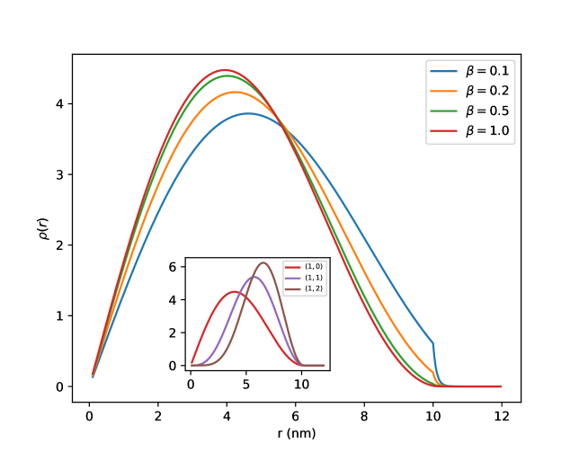
Figure 1: Scaled radial charge density ($rg^{2}(r)$) profile of a QD with R = 10 nm, B = 1 T, and $V_{o}$ = 1 eV. The main plot shows the effect of $\beta$ on the ground state charge density profile. The inset shows the charge density profile of levels (1,0), (1,1) and (1,2) for $\beta$=1. ($m_{o}=m_{e}$, $m_{i}=\beta m_{o}$)

In Fig. 1, we examine the effect of $\beta$ on the ground state charge density profile. We observe that charge spreads out closer to the boundary as $\beta$ is decreased. Further, a small amount of charge leaks out of the QD for small $\beta$ and this is enhanced as $\beta$ is decreased. This is an interesting observation, and can be explained by the fact that the tunnelling probability at the boundary of the QD decays exponentially with the difference $(V_{o}-E)$. As $\beta$ decreases, energy levels rise and the tunnelling probability increases. One can also see the discontinuity in the derivative of $\rho(r)$ at the boundary for small $\beta$, which results from imposing BDD.

The inset in Fig. 1 shows the charge density profile of states (1,0), (1,1) and (1,2). The states $(n,l)$ and $(n,-l)$ have the same charge density since they only differ by an overall phase ($e^{i2l\phi}$). We note that higher energy levels are associated with more spreading of charge towards the boundary. The peak charge density is larger, and is closer to the boundary as we consider higher levels.

4.2 DEPENDENCE OF TRANSITION ENERGIES ON SIZE

Energy difference is the object of study in absorption and emission spectra. Hence, in Fig. (2) we investigate the effect of size, $\beta$, and the magnetic field on the transition energies $(E_{1}-E_{0})$ and $(E_{2}-E_{1})$ (Fig. 2). We observe that $(E_{1}-E_{0})$ decreases with increasing size, while $(E_{2}-E_{1})$ has almost no dependence on size. We fit $(E_{1}-E_{0})\propto 1/R^{\gamma}$ using Levenberg-Marquardt fit. The values of the exponent are found to be $\gamma=1.76$ for $\beta=0.1$ and $\gamma=2.11$ for $\beta=1$. This lateral size confinement effect be explained well by the asymptotic expression we developed in Sec. III. From Eq. (22), we note that the transition energies of interest are determined to be

$$(E_{1}-E_{0})\approx\frac{8.9\hbar^{2}}{2\beta m_{o}R^{2}}\left(1-\frac{1}{\sqrt{\sigma}}\right)^{2}-\frac{\hbar eB_{i}}{\beta m_{o}}$$ (24)

$$(E_{2}-E_{1})\approx\frac{2\hbar eB_{i}}{\beta m_{o}}$$ (25)

From Eq. (23) and Eq. (24), we note that $(E_{1}-E_{0})$ has a $1/R^{2}$ dependence on size, while $(E_{2}-E_{1})$ has no dependence on size. We also examined the effect of $\beta$ on these transition energies. The transition energies have a strong dependence on the magnitude of $\beta$. As evident from Fig. 2, both transition energies increase sharply as $\beta$ is decreased. This is expected from the $1/\beta$ dependence predicted by Eq. (23) and Eq. (24). Transition energy $E_{2}-E_{1}$ increases two times when magnetic field is increased ten times. However, the same transition energy has stronger dependence on BDD condition. Energy $(E_{2}-E_{1})$ is increased seven times on decreasing $\beta$ ten times.

4.3 DEPENDENCE OF ENERGY LEVELS ON MAGNETIC FIELD

Figure 3 shows the energy levels of our system as a function of the applied magnetic field. Interestingly the plots are linear in $B$. This can be understood on the basis of our asymptotic analysis (Eq. (22)). Cyclotron energy ($\hbar\omega_{i}/2$) is manifestly linear in $B$. Additionally a detailed analysis revealed that the first term in Eq. (22) ($1/{\sqrt{\sigma}}$) is also linear in $B$. Thus the exact results also indicate a linear trend of energy on magnetic field.

We observe clear Landau level splitting as the magnetic field is increased. The effect of imposing BDD is again evident from the sharp fall in the energy levels for $\beta=1$. We also find further support for our asymptotic approximation (represented by dashed lines), which converges well with our numerical results for large magnetic field strengths. Asymptotic equation (Eqs. (20) and (22)) points out an important fact. Changing the magnetic field outside does not radically affect the energy of the QD. This can be explained by the fact that probability of finding an electron in the outer region of the dot is very low. If $B_{o}={B_{i}}/{\beta}$ the effect of magnetic field in $\sqrt{\sigma}$ is zero . Which brings out the fact that we can use $B_{o}$ as factor to make $B$ affect $E$ only in terms of the Landau energies. We carried a fit to energy of the form

$$E=\frac{C}{R^{\gamma}}$$ (26)

Table (1) lists the values of the exponent $\gamma$. Interestingly we find that BDD effect reduces $\gamma$. The magnetic field also tends to reduce $\gamma$ but marginally so. This can perhaps be understood as follows: increasing $B$ reduces the cyclotron radius of the electron and hence the electron density at the dot boundary is inconsequential.

$B$ (T)	$\beta$	$\gamma$
0	0.1	1.46
	1.0	1.91
1	0.1	1.56
	1.0	1.91
10	0.1	1.22
	1.0	1.81

Table 1: Investigating the dependence of $E$ on $R$ as $E=C/R^{\gamma}$. Table gives the values of $\gamma$ for various values of $\beta$ and $B$.

4.4 COMPARISON WITH EXPERIMENT

Drexler et. al. [21], in their experiment, used an In_0.5Ga_0.5As-GaAs QD ($m_{i}=0.047m_{e}$ and $m_{o}=0.067m_{e}$, so $\beta\approx 0.7$) with a radius of $(10\pm 1)$ nm. They measured the transition gap $(E_{2}-E_{0})$ as a function of an applied perpendicular magnetic field, and found their data to agree with a parabolic confinement model using $m^{*}=0.07m_{o}$ and $\hbar\omega_{o}=41$ meV. Also, their dots are lens-shaped along the z-axis. However, they mention that their measured transition gap data from IR spectroscopy is decoupled from the high energy z-confinement, and is only due to lateral confinement. The bandgap difference between In_0.5Ga_0.5As and GaAs is about $360$ meV. But this is further split between valence and conduction band offsets, so a realistic value of the barrier height is closer to $100$ meV. In the present work, we have developed a single-electron hard-wall confinement model including BDD within the effective mass framework. It is also important to note that our model is best applicable in a strong confinement regime described by Equations (8) and (9). Using $V_{0}=100$ meV and $\beta=0.7$, we find good agreement with their experimental data for a QD radius of $11$ nm (Figure 4).

In conclusion, we presented a hard-wall confinement based model for a circular Quantum Dot placed in a perpendicular magnetic field. Most importantly, we demonstrated the strong influence of using the BenDaniel-Duke boundary condition on the set of spin-degenerate Landau levels of the system. We also developed a simple asymptotic approximation (Eq. (22)) to the energy levels, which is in fair agreement with numerical results. The agreement is enhanced for larger size and confinement potential. Finally, we also observed that a particular transition gap in our model agrees well with experiments performed on the In_0.5Ga_0.5As-GaAs Quantum Dot [21].

5 ACKNOWLEDGEMENTS

We are extremely thankful to our mentor Praveen Pathak (HBCSE-TIFR) for regular discussions and guidance. We also also thank Vijay Singh (HBCSE-TIFR) for useful discussions. We acknowledge the support of the Govt. Of India, Department of Atomic Energy, under the National Initiative on Undergraduate Science (NIUS) of HBCSE-TIFR (Project No. 12-R&D-TFR-6.04-0600).

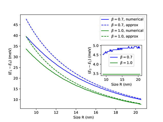
Figure 2: Transition energies as a function of the radius of the QD ($m_{o}$ = 0.067$m_{e}$, $V_{o}$ = 100 meV, B = 1 T) in the range of 10 nm to 20 nm. The main plot shows the effect of size and $\beta$ on the transition gap $(E_{1}-E_{0})$. The inset shows the same for the transition gap $(E_{2}-E_{1})$. The dashed lines in the main plot represent the asymptotic approximation (Eq. (22)). The case of $\beta=0.7$ corresponds to the InGaAs-GaAs QD ($m_{i}$ = 0.047$m_{e}$, $m_{o}$ = 0.067$m_{e}$).

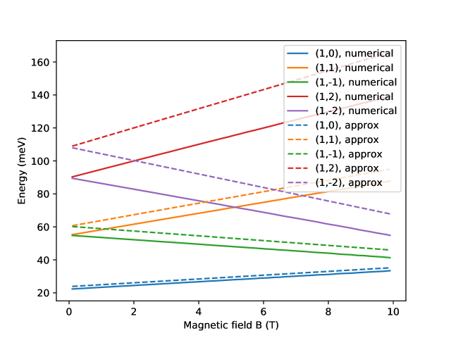
Figure 3: Energy levels of the InGaAs-GaAs QD (R = 11 nm, $V_{o}$ = 100 meV, $m_{o}$ = 0.067$m_{e}$, $\beta$ = 0.7) as a function of an applied magnetic field. The solid lines depict the lowest five levels as obtained from numerical computation. The dashed lines depict the same five levels as expected from our asymptotic approximation (Eq. (22))

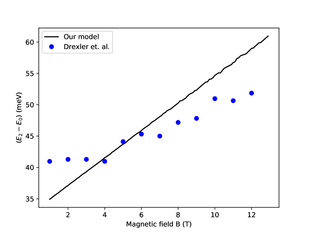
Figure 4: The full line (black) depicts transition energy $(E_{2}-E_{0})$ of the QD ($V_{o}$ = 100 meV, $\beta$ = 0.7, R = 11 nm) as a function of the applied magnetic field. The blue circles are experimental data [21] on the same transition energy for a GaAs-InGaAs QD with R = (10±1) nm. ($m_{i}=0.047m_{e}$, $m_{o}=0.067m_{e}$)

References

- [1] X.-G. Wen, Non-abelian statistics in the fractional quantum hall states, Phy. Rev. Lett. 66 (6) (1991) 802.
- [2] C. Nayak, S. H. Simon, A. Stern, M. Freedman, S. D. Sarma, Non-abelian anyons and topological quantum computation, Rev. Mod. Phy. 80 (3) (2008) 1083.
- [3] R. Ashoori, Electrons in artificial atoms, Nature 379 (6564) (1996) 413.
- [4] M. Veldhorst, J. Hwang, C. Yang, A. Leenstra, B. de Ronde, J. Dehollain, J. Muhonen, F. Hudson, K. M. Itoh, A. Morello, et al., An addressable quantum dot qubit with fault-tolerant control-fidelity, Nature Nanotechnology 9 (12) (2014) 981.
-
[5]
D. Loss, D. P. DiVincenzo,
Quantum computation
with quantum dots, Phys. Rev. A 57 (1998) 120–126.
doi:10.1103/PhysRevA.57.120.
URL https://link.aps.org/doi/10.1103/PhysRevA.57.120 - [6] P. O. Anikeeva, J. E. Halpert, M. G. Bawendi, V. Bulovic, Quantum dot light-emitting devices with electroluminescence tunable over the entire visible spectrum, Nano letters 9 (7) (2009) 2532–2536.
- [7] B. S. Mashford, M. Stevenson, Z. Popovic, C. Hamilton, Z. Zhou, C. Breen, J. Steckel, V. Bulovic, M. Bawendi, S. Coe-Sullivan, et al., High-efficiency quantum-dot light-emitting devices with enhanced charge injection, Nature Photonics 7 (5) (2013) 407.
-
[8]
A. Kurzmann, M. Eich, H. Overweg, M. Mangold, F. Herman, P. Rickhaus,
R. Pisoni, Y. Lee, R. Garreis, C. Tong, K. Watanabe, T. Taniguchi,
K. Ensslin, T. Ihn,
Excited states
in bilayer graphene quantum dots, Phys. Rev. Lett. 123 (2019) 026803.
doi:10.1103/PhysRevLett.123.026803.
URL https://link.aps.org/doi/10.1103/PhysRevLett.123.026803 - [9] P. Harrison, A. Valavanis, Quantum wells, wires and dots: theoretical and computational physics of semiconductor nanostructures, John Wiley & Sons, 2016.
-
[10]
Ivanov et. al,
Type-II core/shell CdS/ZnSe nanocrystals: Synthesis, electronic structures, and spectroscopic properties, J. Am. Chem. Soc. 2007, 129, 38, 11708–11719
doi:10.1021/ja068351m
URL https://pubs.acs.org/doi/abs/10.1021/ja068351m -
[11]
M. Tkach, J. Seti, O. Voitsekhivska,
Spectrum
of electron in quantum well within the linearly-dependent effective mass
model with the exact solution, Superlattices and Microstructures 109 (2017)
905 – 914.
doi:https://doi.org/10.1016/j.spmi.2017.06.013.
URL http://www.sciencedirect.com/science/article/pii/S0749603617311941 -
[12]
D. J. BenDaniel, C. B. Duke,
Space-charge effects
on electron tunneling, Phys. Rev. 152 (1966) 683–692.
doi:10.1103/PhysRev.152.683.
URL https://link.aps.org/doi/10.1103/PhysRev.152.683 - [13] M. Singh, V. Ranjan, V. A. Singh, The role of the carrier mass in semiconductor quantum dots, Int. J. of Mod. Phy. B 14 (17) (2000) 1753–1765.
- [14] V. A. Singh, L. Kumar, Revisiting elementary quantum mechanics with the bendaniel-duke boundary condition, Am. J. Phy. 74 (5) (2006) 412–418.
- [15] S. Singh, P. Pathak, V. A. Singh, Approximate approaches to the one-dimensional finite potential well, Eur. J. Phy. 32 (6) (2011) 1701.
-
[16]
F. Koc, K. Koksal,