Exact solution of the Boltzmann equation for low-temperature transport coefficients in metals II: Scattering by ferromagnons

Abstract

In a previous paper (Paper I) we developed a technique for exactly solving the linearized Boltzmann equation for the electrical and thermal transport coefficients in metals in the low-temperature limit. Here we adapt this technique to determine the magnon contribution to the electrical and thermal conductivities, and to the thermopower, in metallic ferromagnets. For the electrical resistivity $\rho$ at asymptotically low temperatures we find $\rho\propto\exp{(-T_{\text{min}}/T)}$, with $T_{\text{min}}$ an energy scale that results from the exchange gap and a temperature independent prefactor of the exponential. The corresponding result for the heat conductivity is $\sigma_{h}\propto T^{3}\,\exp{(T_{\text{min}}/T)}$, and thermopower is $S\propto T$. All of these results are exact, including the prefactors.

I Introduction

The scattering of conduction electron in metals by soft excitations, and the resulting temperature dependence of the transport coefficients in the low-temperature ($T\to 0$) limit is an old problem. The best known example is Bloch’s $T^{5}$ law for the electrical resistivity due to the scattering by acoustic phonons.Bloch (1930); Ziman (1960) In magnetic metals, the magnetic Goldstone modes also contribute to the scattering. Magnons in antiferromagnets yield a $T^{5}$ contribution as phonons do,Yamada and Takada (1974); Ueda (1977) whereas the corresponding result for helimagnets is $T^{5/2}$.Belitz et al. (2006)

Within magnetic systems, ferromagnets are a special case in that only electron scattering between different sub-bands of the exchange-split conduction band is possible. This leads to a lower limit $T_{\text{min}}$ on the energy transfer, with the temperature scale $T_{\text{min}}$ determined by the exchange splitting and the spin-stiffness coefficient. For temperatures large compared to $T_{\text{min}}$, Ueda and MoriyaUeda and Moriya (1975) found that scattering by ferromagnons yield a $T^{2}$ contribution to the electrical resistivity. For $T\ll T_{\text{min}}$ the electrical resistivity $\rho$ is exponentially small and has the formBharadwaj et al. (2014)

$$\rho=\frac{m}{ne^{2}}\,T_{1}\,r(T)\,e^{-T_{\text{min}}/T}\ .$$ (1a)

Here $$m n e T_{1} r r(T)\propto(T/T_{1})^{2}$$, , and are the electron mass, number density, and charge, respectively. is the magnetic Debye temperature, and the dimensionless function is a power-law function of its argument. By evaluating the Kubo formula in a conserving approximation, Ref. Bharadwaj et al., 2014 found .

All of the above results were obtained by solving either the linearized Boltzmann equation, or an equivalent integral equation derived from the Kubo formula, in an uncontrolled approximation that replaces various energy-dependent relaxation rates by constants, see Ref. Mahan, 2000 for the electron-phonon case. Only very recently has it been shown that a mathematically rigorous solution of the integral equation does indeed yield the Bloch $T^{5}$ law for the case of electron-phonon scattering.Amarel et al. (2020) In a previous paperPap (to be referred to as Paper I) we have simplified and extended the method of Ref. Amarel et al., 2020. We have shown that the heat conductivity and the thermopower can also be determined exactly, and we have applied the method to electron scattering by antiferromagnons and helimagnons in addition to phonons. In all of these cases, it turned out that the uncontrolled approximation affected the prefactor of the temperature dependence of the transport coefficients, but the functional form of the various $T$-dependence was exact. It is the purpose of the present paper to show that in ferromagnets the situation is different: an exact solution of the integral equation yields a prefactor $r$ in Eq. (1a) that is constant in the limit $T\to 0$,

$$r(T)=8g_{0}\,\frac{T_{0}^{3}}{T_{1}\lambda}\left[1+O(T\lambda/T_{0}^{2})\right]\ .$$ (1b)

Here $T_{0}$ is a temperature scale that is closely related to $T_{\text{min}}$, $\lambda$ is the exchange splitting, and $g_{0}$ is a dimensionless coupling constant that depends on the magnetization. The corresponding result for the thermopower $S$ is

$$S(T\to 0)=\frac{-\pi^{2}}{6e}\,\frac{T}{\epsilon_{\text{F}}}\ ,$$ (2)

which is the same as for scattering by phonons, antiferromagnons, or helimagnons. The prefactors in Eqs. (1b) and (2) are exact. The result for the heat conductivity is

$$\sigma_{h}(T\to 0)\propto(T^{3}/T_{0}^{3})\,e^{T_{\text{min}}/T}\ ,$$ (3)

but the numerical prefactor cannot be determined in closed form.

This paper is organized as follows. In Sec. II we recall the linearized Boltzmann equations for the magnon scattering contributions to the electrical and thermal resistivities, as well as for the thermopower. In Sec. III we adapt the method from Paper I to solve the Boltzmann equation exactly in the limit of asymptotically low temperature. We conclude in Sec. IV with a summary and a discussion of our results. Appendix A summarizes the derivation of the effective scattering potential, and the derivation of the linearized Boltzmann equations from the Kubo formulas. Appendix B lists various relaxation rates, and Appendix C contains some technical details regarding the spectral analysis of the collision operator.

II Kinetic equations for transport coefficients in ferromagnets

II.1 Energy scales, and transport coefficients

We start by recalling some well known aspects of metallic ferromagnets. Their origins have been discussed in detail in Ref. Bharadwaj et al., 2014, and we will just state the results.

In a ferromagnet, the magnetic order splits the conduction band into two sub-bands that are separated by the exchange splitting $\lambda$ and can be indexed by the spin projection index $\sigma=\pm 1$. Let $\mu$ be the chemical potential, $\mu(T=0)=\epsilon_{\text{F}}$ the Fermi energy, $k_{\text{F}}$ the Fermi wave number in the non-magnetic state, and $m$ the electron effective mass. Then the Fermi wave numbers of the sub-bands are $k_{\text{F}}^{\sigma}=k_{\text{F}}\sqrt{1+\sigma\lambda/\mu}$ and the corresponding densities of states are $N_{\text{F}}^{\sigma}=k_{\text{F}}^{\sigma}m/2\pi^{2}$. The Goldstone mode associated with the magnetic order is the ferromagnon, with a frequency-momentum relation

$$\omega_{\bm{k}}=D{\bm{k}}^{2}\ ,$$ (4)

with $D$ the spin-wave stiffness coefficient.mag There are two relevant energy scales in addition to the Fermi energy. One is the magnetic Debye temperature

$$T_{1}=Dk_{\text{F}}^{2}\ .$$ (5)

The other one is a temperature scale $T_{0}$ that is related to the minimum momentum transfer in scattering processes between the two sub-bands that are mediated by ferromagnons,

$$T_{0}=\frac{1}{4}\,D(k_{\text{F}}^{+}-k_{\text{F}}^{-})^{2}=\frac{1}{4}\,T_{1}(\lambda/\epsilon_{\text{F}})^{2}$$ (6)

A crucial feature of the coupling of ferromagnons to conduction electrons is that the magnons couple only electrons in different sub-bands (‘interband coupling’). This is in contrast to antiferromagnets and helimagnets, where the Goldstone modes can couple electrons in the same sub-band (‘intraband coupling’), see Paper I. As a result, the energy scale $T_{0}$ plays an important role for transport processes: For temperatures $T<T_{0}$ the magnon-induced scattering processes get frozen out, and all transport coefficients will show an exponential temperature dependence with the temperature scale set by $T_{0}$.

To define the transport coefficients we consider a mass current ${\bm{J}}$ and a heat current ${\bm{J}}_{h}$ driven by gradients of the electrochemical potential $\bar{\mu}=\mu+eV$ and the temperature $T$, respectively. Here $e$ is the electron charge, and $V$ is the electric potential. To linear order in the potential gradients the currents are determined by three independent transport coefficients (see, e.g., Ref. Mahan, 2000),

$${\bm{J}}=-\frac{1}{T}\,L_{11}\bm{\nabla}\bar{\mu}-\frac{1}{T^{2}}\,L_{12}\,\bm{\nabla}T\ ,$$ (7a)

$${\bm{J}}_{h}=-\frac{1}{T}\,L_{12}\bm{\nabla}\bar{\mu}-\frac{1}{T^{2}}\,L_{22}\,\bm{\nabla}T\ .$$ (7b)

An Onsager relation ensures that the same coefficient $L_{12}$ appears in both Eq. (7a) and (7b). The electrical conductivity $\sigma$ is defined for the case of constant temperature and constant chemical potential, via $e{\bm{J}}=-\sigma\bm{\nabla}V$. Analogously, the heat conductivity $\sigma_{h}$ for a constant electrochemical potential is defined via ${\bm{J}}_{h}=-\sigma_{h}\bm{\nabla}T$. We therefore have

$$\sigma=\frac{e^{2}}{T}\,L_{11}\quad,\quad\sigma_{h}=\frac{1}{T^{2}}\,L_{22}\ .$$ (8a)

The thermopower or Seebeck coefficient $$S \bm{\nabla}V=S\,\bm{\nabla}T$$ is defined in the absence of a mass current via , and hence

$$-eS=\frac{1}{T}\,\frac{L_{12}}{L_{11}}\ .$$ (8b)

What is usually measured, rather than $$\sigma_{h} \kappa$$, is the heat conductivity in the absence of a mass current. It is given by

$$\kappa = \frac{1}{T^{2}}\left(L_{22}-(L_{12})^{2}/L_{11}\right)$$ (8c)

$$= \sigma_{h}-T\,S^{2}\,\sigma\ .$$

The three transport coefficients can all be expressed in terms of energy and spin dependent relaxation functions $\varphi_{0}$ and $\varphi_{1}$,

$$\sigma = \frac{e^{2}}{2m}\sum_{\sigma}n_{\sigma}\,\frac{1}{T}\int d\epsilon\,w(\epsilon)\,\varphi_{0}^{\sigma}(\epsilon)\ ,\hskip 30.0pt$$ (9a)

$$-ST\sigma/e = \frac{1}{2m}\sum_{\sigma}n_{\sigma}\,\frac{1}{T}\int d\epsilon\,w(\epsilon)\,\varphi_{1}^{\sigma}(\epsilon)\ ,$$ (9b)

$$T\sigma_{h} = \frac{1}{2m}\sum_{\sigma}n_{\sigma}\,\frac{1}{T}\int d\epsilon\,w(\epsilon)\,\epsilon\,\varphi_{1}^{\sigma}(\epsilon)\ .$$ (9c)

Here $n_{\sigma}$ is the electron density for spin projection $\sigma$. Here, and throughout this paper, we denote by $\int d\epsilon$ a definite integral over all real values of $\epsilon$. The weight function $w$ is given in terms of the Fermi function $f_{0}(x)=1/(e^{x}+1)$, i.e., the equilibrium distribution function of the electrons,

$$w(\epsilon)=f_{0}(\epsilon/T)\left[1-f_{0}(\epsilon/T)\right]=\frac{1}{\cosh^{2}(\epsilon/T)}$$ (10a)

with a normalization

$$\int d\epsilon\,w(\epsilon)=T\ .$$ (10b)

$\varphi_{0}$ is dimensionally an inverse energy, and physically a relaxation time. $\varphi_{1}$ is dimensionless. $\varphi_{0}$ and $\varphi_{1}$ are determined as the solutions of kinetic equations that we discuss next.

II.2 Kinetic equations

The integrals on the right-hand sides of Eqs. (9) can be written as Kubo expressions for the particle-number current – particle-number current, particle-number current – heat current, and heat current – heat current correlations, respectively.Kubo (1957); Mahan (2000) The Kubo formulas give the exact linear response of the system, and are very hard to evaluate. They are usually analyzed by means of a conserving approximation that is equivalent to the linearized Boltzmann equation,Mahan (2000) and the non-equilibrium aspects of the bosons (in our case, the ferromagnons) are ignored for simplicity. Even this procedure leads to singular integral equations of Fredholm type that are hard to solve. The relevant integral equation for the function $\varphi_{0}$ that determines the electrical conductivity was derived in Ref. Bharadwaj et al., 2014; the main steps of that derivation are summarized in Appendix A. The analogous equations for $\varphi_{1}$ is obtained via the same procedure by replacing the number current with the heat current. The result can be written in the form

$$\Lambda^{\sigma}(\epsilon)\,\varphi_{0}^{\sigma}(\epsilon) = -1\ ,$$ (11a)

$$\Lambda^{\sigma}(\epsilon)\,\varphi_{1}^{\sigma}(\epsilon) = -\epsilon\ .$$ (11b)

Here $\Lambda^{\sigma}(\epsilon)$ is a collision operator that is defined as

$$\Lambda^{\sigma}(\epsilon)=\int du\sum_{\sigma^{\prime}}\left[K^{\sigma\sigma^{\prime}}(\epsilon,u)\,R_{\epsilon\to u}^{\sigma\to\sigma^{\prime}}-K_{0}^{\sigma\sigma^{\prime}}(\epsilon,u)\right]\ ,$$ (12)

with

$$R_{\epsilon\to u}^{\sigma\to\sigma^{\prime}}f^{\sigma}(\epsilon)=f^{\sigma^{\prime}}(u)$$ (13)

for any spin-dependent function $f^{\sigma}(\epsilon)$. The kernel $K$ has five contributions:Bharadwaj et al. (2014); K (34); mag

$$K^{\sigma\sigma^{\prime}}(\epsilon,u) = K_{0}^{\sigma\sigma^{\prime}}(\epsilon,u)+K_{1}^{\sigma\sigma^{\prime}}(\epsilon,u)+K_{2}^{\sigma\sigma^{\prime}}(\epsilon,u)$$ (14)

$$+K_{3}^{\sigma\sigma^{\prime}}(\epsilon,u)+K_{4}^{\sigma\sigma^{\prime}}(\epsilon,u)\ ,$$

from which one can construct relaxation rates

$$\Gamma_{n}^{\sigma}(\epsilon)=\int du\sum_{\sigma^{\prime}}K_{n}^{\sigma\sigma^{\prime}}(\epsilon,u)\quad(n=0,1,2,3,4)\ ,$$ (15)

The basic ingredient of the kernel is $K_{0}$, all other parts can be expressed in terms of it. It can be writtenBharadwaj et al. (2014)

$$K_{0}^{\sigma\sigma^{\prime}}(\epsilon,u)=N_{\text{F}}^{\sigma^{\prime}}\left[n_{0}\left(\frac{u-\epsilon}{T}\right)+f_{0}\left(\frac{u}{T}\right)\right]V_{\sigma\sigma^{\prime}}(u-\epsilon)\ ,$$ (16a)

where $$n_{0}(x)=1/(e^{x}-1) V$$ is the Bose distribution function. The effective potential reads

$$V_{\sigma\sigma^{\prime}}(u) = -\sigma(1-\delta_{\sigma\sigma^{\prime}})\,\frac{g_{0}}{N_{\text{F}}}\,\Theta(-\sigma u)$$ (16b)

$$\times\Theta(|u|-T_{\text{min}})\,\Theta(T_{1}-|u|)\ .\qquad$$

The spin structure of this expression shows explicitly that the potential couples only electrons in different sub-bands of the split conduction band. The lower energy cutoff $T_{\text{min}}$ is a result of this structure, and it will obviously be closely related to $T_{0}$ as defined in Eq. (6). For $T_{1}\approx\lambda\ll\epsilon_{\text{F}}$, which is always true in metals, one finds

$$T_{\text{min}}=T_{0}\left[1+T_{0}\left(\frac{1}{T_{1}}+\frac{1}{\lambda}\right)\right]+O\left(\frac{T_{0}^{3}}{T_{1}},\frac{T_{0}^{3}}{T_{1}\lambda},\frac{T_{0}^{3}}{\lambda^{2}}\right)\ .$$ (17)

Here we ignore a spin dependence of the lower frequency cutoff that becomes relevant only at unrealizably low temperatures. The final step function in Eq. (16b) reflects the upper energy cutoff provided by the magnetic Debye temperature $T_{1}$, and $g_{0}$ is a dimensionless coupling constant that is proportional to the residue of the ferromagnon pole, which in turn is related to the magnetization.g0_

The kernels $K_{1}$ through $K_{4}$ are related to $K_{0}$ via

$$K_{1}^{\sigma\sigma^{\prime}}(\epsilon,u) = \frac{-2\sqrt{T_{0}/T_{1}}}{1-4T_{0}/T_{1}}\,\sigma\,K_{0}^{\sigma\sigma^{\prime}}(\epsilon,u)$$ (18a)

$$K_{2}^{\sigma\sigma^{\prime}}(\epsilon,u) = \frac{-2}{1-4T_{0}/T_{1}}\left(\frac{|u-\epsilon|}{T_{1}}-\frac{2T_{0}}{T_{1}}\right)\,$$

$$\hskip 80.0pt\times K_{0}^{\sigma\sigma^{\prime}}(\epsilon,u)\ ,$$

$$K_{3}^{\sigma\sigma^{\prime}}(\epsilon,u) = \frac{\sqrt{T_{0}/T_{1}}}{1-4T_{0}/T_{1}}\left(\frac{u-\epsilon}{\lambda}+\frac{4|u-\epsilon|}{T_{1}}\,\sigma\right)\,$$

$$\hskip 80.0pt\times K_{0}^{\sigma\sigma^{\prime}}(\epsilon,u)\ ,$$

$$K_{4}^{\sigma\sigma^{\prime}}(\epsilon,u) = \frac{-2T_{0}/T_{1}}{1-4T_{0}/T_{1}}\,\frac{u-\epsilon}{\lambda}\,\sigma\,K_{0}^{\sigma\sigma^{\prime}}(\epsilon,u).\$$ (18d)

They give rise to five separate parts of the collision operator defined by

$$\Lambda_{0}^{\sigma}(\epsilon) = \int du\sum_{\sigma^{\prime}}\left[K_{0}^{\sigma\sigma^{\prime}}(\epsilon,u)\,R_{\epsilon\to u}^{\sigma\to\sigma^{\prime}}-K_{0}^{\sigma\sigma^{\prime}}(\epsilon,u)\right]\ ,$$

$$\Lambda_{i}^{\sigma}(\epsilon) = \int du\sum_{\sigma^{\prime}}K_{i}^{\sigma\sigma^{\prime}}(\epsilon,u)\,R_{\epsilon\to u}^{\sigma\to\sigma^{\prime}}\quad(i=1,2,3,4)\ ,$$

and the full collision operator is given by

$$\Lambda=\Lambda_{0}+\Lambda_{1}+\Lambda_{2}+\Lambda_{3}+\Lambda_{4}\ .$$ (19c)

We have written the integral equations (11) in a form that is standard in kinetic theory.Dorfman et al. (2021) Their derivation from the Kubo formulas, and their relation to the form usually used in many-body theory, is explained in Appendix A.

II.3 Properties of the collision operator

In order to consider the symmetry properties of the kernels $K_{i}$ we define a spin-dependent weight function

$$w_{\sigma}(\epsilon)=w(\epsilon)\,w_{\sigma}$$ (20a)

with $$w(\epsilon)$$ from Eq. (10a) and

$$w_{\sigma}=\frac{1}{\nu}\,\left(k_{\text{F}}^{\sigma}/k_{\text{F}}\right)=\frac{1}{\nu}\,(1+\sigma\lambda/\epsilon_{\text{F}})^{1/2}$$ (20b)

where

$$\nu=\sum_{\sigma}(1+\sigma\lambda/\epsilon_{\text{F}})^{1/2}$$ (20c)

so that

$$\int d\epsilon\sum_{\sigma}w_{\sigma}(\epsilon)=T\ .$$ (20d)

The kernels then obey

$$w_{\sigma}(\epsilon)\,K_{0,2,4}^{\sigma\sigma^{\prime}}(\epsilon,u) = w_{\sigma^{\prime}}(u)\,K_{0,2,4}^{\sigma^{\prime}\sigma}(u,\epsilon)\ ,$$ (21a)

$$w_{\sigma}(\epsilon)\,K_{1,3}^{\sigma\sigma^{\prime}}(\epsilon,u) = -w_{\sigma^{\prime}}(u)\,K_{1,3}^{\sigma^{\prime}\sigma}(u,\epsilon)\ ,\quad$$ (21b)

We further define a scalar product in the space of real-valued functions by

$$\langle\psi|\varphi\rangle=\int d\epsilon\sum_{\sigma}w_{\sigma}(\epsilon)\,\psi^{\sigma}(\epsilon)\,\varphi^{\sigma}(\epsilon)\ ,$$ (22)

Equations (21) then imply that the collision operators $\Lambda_{0,2,4}$ are self-adjoint with respect to this scalar product, whereas $\Lambda_{1,3}$ are skew-adjoint. It is further useful to define averages with respect to the weight function $w_{\sigma}$ by

$$\langle\varphi\rangle_{w_{\sigma}}=\frac{1}{T}\int d\epsilon\,w_{\sigma}(\epsilon)\,\varphi_{\sigma}(\epsilon)=\langle 1|\varphi\rangle/\langle 1|1\rangle\ .$$ (23)

The integral equations (11) can now be written

$$\Lambda|\varphi_{0}\rangle = -|1\rangle\ ,$$ (24a)

$$\Lambda|\varphi_{1}\rangle = -|\epsilon\rangle\ ,$$ (24b)

where $|1\rangle$ represents the constant function that is identically equal to one, and $|\epsilon\rangle$ represents the linear function $f(\epsilon)=\epsilon$. In particular, the normalization of the weight function, Eq. (20d), now takes the form

$$\langle 1|1\rangle=T\ ,$$ (25)

and the transport coefficients from Eqs. (19) can be written

$$\sigma = \frac{ne^{2}}{mT}\,\langle\varphi_{0}|1\rangle\ ,$$ (26a)

$$-ST\sigma/e = \frac{n}{mT}\,\langle\varphi_{1}|1\rangle\ ,$$ (26b)

$$T\sigma_{h} = \frac{n}{mT}\,\langle\varphi_{1}|\epsilon\rangle\ .$$ (26c)

$\Lambda_{0}$ has a zero eigenvalue with the constant function as the eigenfunction. This is true by construction: From Eq. (LABEL:eq:2.16a) we immediately obtain

$$\Lambda_{0}|1\rangle=0\ .$$ (27)

The physical meaning of this zero eigenvalue is the approximate conservation law for the electron momentum in the limit $T\to 0$, where the momentum transfer due to magnons is frozen out. The zero eigenvalue has multiplicity one, and all other eigenvalues are negative. The proof of these statements is exactly analogous to the proof given in Sec. II.B.3 of Paper I for the electron-phonon case.

All of the above is an obvious generalization of the formalism developed in Paper I. Also following Paper I, we assume that the collision operator $\Lambda$ has a spectral representation

$$\Lambda=\sum_{n}\mu_{n}\,\frac{|e_{n}\rangle\langle e_{n}|}{\langle e_{n}|e_{n}\rangle}$$ (28)

with eigenvalues $\mu_{n}$ and a complete orthogonal set of right eigenvectors $|e_{n}\rangle$ and left eigenvectors $\langle e_{n}|$,LR_ so the unit operator is represented by

$$\mathbbm{1}=\sum_{n}\frac{|e_{n}\rangle\langle e_{n}|}{\langle e_{n}|e_{n}\rangle}\ .$$ (29)

In the following section we will use this spectral representation to construct exact solutions of the integral equations (24). As in Paper I, we will need to distinguish between the ‘hydrodynamic’ part of the function $\varphi_{1}$, which is related to the perturbed zero eigenvalue of the collision operator, and the ‘non-hydrodynamic’ or ‘kinetic’ part that is unrelated to the zero eigenvalue. To lowest order in our expansion, the kinetic part is given by $|h\rangle$, which is the solution of

$$\Lambda_{0}|h\rangle=-|\epsilon\rangle\ .$$ (30)

This equation has a solution since the inhomogeneity is orthogonal to the zero eigenvector, $\langle\epsilon|1\rangle=0$.

III Solutions of the kinetic equations

In this section we construct formally exact solutions of the kinetic equations (11). Our technique for doing so is modeled after the analysis of the electron-phonon scattering problem in Paper I, which in turn is based on a mathematically rigorous treatment that was given in Ref. Amarel et al., 2020. What makes the exact solution possible is the zero eigenvalue of the collision operator $\Lambda_{0}$, see Eq. (27). The other parts of the collision operator in Eq. (19c) perturb the zero eigenvalue. If $T$ and $T_{0}$ are both small compared to the magnetic Debye temperature $T_{1}$, these perturbations are small and allow for a controlled determination of the smallest eigenvalue, which dominates the transport coefficients. A complication compared to Paper I arises from the fact that the potential that governs the effective electron-electron interaction, $V$ in Eq. (16b), is gapped, and care must be taken to distinguish between powers of $T$ and powers of $T_{\text{min}}\approx T_{0}$.

III.1 Solutions of the integral equations

III.1.1 Scaling considerations

We are interested in the behavior in the low-temperature regime defined by $T\ll T_{0}$. Accordingly, we introduce a small parameter $\alpha$ that scales as $\alpha\sim\sqrt{T/T_{1}}\ll 1$ that counts powers of temperature. Only even powers of $\alpha$ will occur in the low-temperature expansion. In addition, we assume that $\lambda/\epsilon_{\text{F}}\approx T_{1}/\epsilon_{\text{F}}\ll 1$, and associate another small counting parameter $\beta\sim T_{1}/\epsilon_{\text{F}}\sim\sqrt{T_{0}/T_{1}}$ with this energy ratio. (This is true in metals, but not necessarily in, e.g., magnetic semiconductors.) $\lambda$ and $T_{1}$ are physically different energy scales, but their values are usually of the same order and we will not distinguish between them for scaling purposes. An inspection of the kernels, Eqs. (16 - 18), shows that the collision operators $\Lambda_{n}$ scale, to leading order, as $\Lambda_{n}\sim\beta^{n+2}$. Futhermore, matrix elements that involve the vector $|\epsilon\rangle$ scale as $\langle\epsilon|\Lambda_{n}|\epsilon\rangle/T\sim\beta^{n+2}$, since only the $\epsilon$-integration measure scales as the temperature, which gets canceled by the normalization factor $1/T$. Corrections to the leading scaling behavior involve powers of $\alpha\sim\sqrt{T/T_{1}}$, which for $T\ll T_{0}$ are small compared to $\beta\sim\sqrt{T_{0}/T_{1}}$ to the same power. As a simple example, consider the average of the rate $\Gamma_{0}$, Eq. (15), that is calculated in Appendix A. The result is

$$\langle\Gamma_{0}\rangle_{w_{\sigma}}\propto(T_{\text{min}}+T)e^{-T_{\text{min}}/T}\ ,$$ (31a)

and the leading scaling behavior thus is

$$\langle\Gamma_{0}\rangle_{w_{\sigma}}\sim\beta^{2}+\alpha^{2}\ .$$ (31b)

In general, for temperatures $T\ll T_{0}$ the $T_{0}$-scaling will dominate, and the only temperature dependence of observables, other than the leading exponential one, will result from factors such as $\langle\epsilon^{2}\rangle_{w{\sigma}}\propto T^{2}$ that do not involve the collision operator. There is, however, one exception to this conclusion: Suppose an observable $\cal O$ scales as $\beta^{2n}$ plus corrections, but the leading term has a zero prefactor:

$${\cal O}\sim 0\times\beta^{2n}+\beta^{2n-2}\alpha^{2}+\beta^{2n+2}+O(\beta^{2n-4}\alpha^{4},\beta^{2n}\alpha^{2})\ .$$ (32)

Then $\alpha^{2}$ competes with $\beta^{4}$ rather than $\beta^{2}$, and thus the leading $\alpha$-correction dominates over the leading nonzero $\beta$-scaling for temperatures $T_{0}^{2}/T_{1}<T<T_{0}$, and has to be kept. As we will see, this does indeed happen. In all cases where the coefficient of the leading $\beta$-scaling term is nonzero, on the other hand, we can neglect all temperature corrections.

We now write the collision operator as

$$\Lambda=\beta^{2}\Lambda_{0}+\beta^{3}\Lambda_{1}+\beta^{4}\Lambda_{2}+\beta^{5}\Lambda_{3}+\beta^{6}\Lambda_{4}\ ,$$ (33)

where powers $\beta^{n}$ imply that the corresponding part of the collision operator scales at least as $(T_{1}/\epsilon_{\text{F}})^{n}\sim(\lambda/\epsilon_{\text{F}})^{n}$, or $(T_{0}/T_{1})^{n/2}$. Forming matrix elements with these collision operators will lead to $\alpha$-corrections to the leading scaling behavior, which we will keep as needed. These scaling behaviors all pertain to the prefactor of the exponential $\exp(-T_{\text{min}}/T)$. In the end, we will put $\beta=1$.

III.1.2 The inverse collision operator

We now proceed in analogy to Paper I. That is, we expand the lowest eigenvalue $\mu_{0}$ and the corresponding eigenvector $|e_{0}\rangle$ in power series in $\beta$,

$$\mu_{0}=\beta^{2}\mu_{0}^{(0)}+\beta^{3}\mu_{0}^{(1)}+\beta^{4}\mu_{0}^{(2)}+O(\beta^{5})\ ,$$ (34a)

$$|e_{0}\rangle=|e_{0}^{(0)}\rangle+\beta|e_{0}^{(1)}\rangle+\beta^{2}|e_{0}^{(2)}\rangle+O(\beta^{3})$$ (34b)

and solve the eigenproblem

$$\Lambda|e_{0}\rangle=\mu_{0}|e_{0}\rangle$$ (35)

order by order in $\beta$. This will allow us to construct the leading behavior of the inverse collision operator, $\Lambda^{-1}$, which in turn will yield the leading contributions to the solutions of the integral equations (24). As mentioned above, the various parts of the collision operator, and hence the eigenvalues and eigenvectors, contain powers of $\sqrt{T_{0}/T_{1}}$ equal to or higher than the one indicated by the power of $\beta$ in Eqs. (33) and (34). Rather than keeping explicit powers of $\beta$ everywhere, we will therefore use $\beta$ interchangeably with $\sqrt{T_{0}/T_{1}}$, and $\alpha$ with $\sqrt{T/T_{1}}$, mostly to indicate leading scaling behavior, and higher-order corrections. At all times we will maintain a systematic double expansion in powers of $\beta\sim\sqrt{T_{0}/T_{1}}$ and $\alpha\sim\sqrt{T/T_{1}}$.

Identities that will be useful in this context are

$$\Lambda_{0}|1\rangle = 0\ ,$$ (36a)

$$\Lambda_{1}|1\rangle = \frac{\sqrt{T_{0}/T_{1}}}{1-4T_{0}/T_{1}}\,\Lambda_{0}|\sigma\rangle$$ (36b)

$$\Lambda_{1}|\sigma\rangle = \frac{-\sqrt{T_{0}/T_{1}}}{1-4T_{0}/T_{1}}\,\sigma\Lambda_{0}|\sigma\rangle$$ (36c)

$$\Lambda_{2}|1\rangle = \frac{2/T_{1}}{1-4T_{0}/T_{1}}\,\sigma\Lambda_{0}|\epsilon\rangle-\frac{2T_{0}/T_{1}}{1-4T_{0}/T_{1}}\,\sigma\Lambda_{0}|\sigma\rangle$$

$$\Lambda_{2}|\sigma\rangle = \frac{-2/T_{1}}{1-4T_{0}/T_{1}}\,\Lambda_{0}|\epsilon\rangle+\frac{2T_{0}/T_{1}}{1-4T_{0}/T_{1}}\,\Lambda_{0}|\sigma\rangle$$

$$\Lambda_{3}|1\rangle = \frac{\sqrt{T_{0}/T_{1}}}{1-4T_{0}/T_{1}}\left(\frac{1}{\lambda}-\frac{4}{T_{1}}\right)\Lambda_{0}|\epsilon\rangle\ .$$ (36f)

Here $|\sigma\rangle$ represents the function $f^{\sigma}(\epsilon)=\sigma$, and $\sigma\Lambda_{0}$ denotes the collision operator constructed from the kernel $\sigma K_{0}^{\sigma\sigma^{\prime}}(\epsilon,u)$.

To lowest (i.e., quadratic) order in $\beta$ we have, by construction,

$$\mu_{0}^{(0)} = 0\ ,$$ (37a)

$$|e_{0}^{(0)}\rangle = |1\rangle\quad,\quad\langle e_{0}^{(0)}|=\langle 1|\ .$$ (37b)

This is the zero eigenvalue that was mentioned in Sec. II.3.

To next-leading order the eigenequation reads

$$\Lambda_{0}|e_{0}^{(1)}\rangle+\Lambda_{1}|1\rangle=\mu_{0}^{(1)}|1\rangle\ .$$ (38)

Multiplying from the left with $\langle 1|$ yields

$$\mu_{0}^{(1)}=0\ .$$ (39a)

To find the corresponding eigenvector we use Eq. (36b), which implies

$$|e_{0}^{(1)}\rangle = \frac{-\sqrt{T_{0}/T_{1}}}{1-4T_{0}/T_{1}}\,|\sigma\rangle+\frac{1}{2}\,\frac{1-\sqrt{1-4T_{0}/T_{1}}}{1-4T_{0}/T_{1}}\,|1\rangle\ .$$

$$= -\left(\frac{T_{0}}{T_{1}}\right)^{1/2}\left[1+O(\beta^{2}\right)]|\sigma\rangle+\frac{T_{0}}{T_{1}}\left[1+O(\beta^{2})\right]|1\rangle\ .$$

Note that an arbitrary multiple of the zero eigenfunction $|1\rangle$ can be added to $|e_{0}^{(1)}\rangle$; Eq. (LABEL:eq:3.9b) reflects the fact that $|e_{0}^{(1)}\rangle$ should be orthogonal to $|1\rangle$. We use the same notation for the right and left eigenfunctions as in Sec. II.3, and it comes with the same caveats.LR_ Accordingly, the left even eigenvectors $\langle e_{0}^{(2n)}|$ represent the same functions as the corresponding right eigenvectors $|e_{0}^{(2n)}\rangle$, whereas the left odd eigenvectors $\langle e_{0}^{(2n+1)}|$ represent minus the functions represented by the $|e_{0}^{(2n+1)}\rangle$. This is a consequence of the skew-adjointness of the operators $\Lambda_{2n+1}$.

To order $\beta^{4}$, the equation

$$\Lambda_{0}|e_{0}^{(2)}\rangle+\Lambda_{1}|e_{0}^{(1)}\rangle+\Lambda_{2}|1\rangle=\mu_{0}^{(2)}|1\rangle$$ (40)

yields, for the eigenvalue,

$$\mu_{0}^{(2)}=\langle\Gamma_{2}\rangle_{w_{\sigma}}-\frac{2T_{0}/T_{1}}{(1-4T_{0}/T_{1})^{2}}\langle\Gamma_{0}\rangle_{w_{\sigma}}\ .$$ (41a)

A calculation of the average rates, see Appendix A, shows that the leading contributions, i.e., the ones that scale as $$\beta^{4}\sim(T_{0}/T_{1})^{2} K_{2} K_{0} |u-\epsilon| K_{2} T_{0}/T_{1} \beta^{2}\alpha^{2}\sim T_{0}T/T_{1}^{2}$$, cancel between the two terms. This is also obvious from the relation (80a) (see also Eq. (LABEL:eq:2.15b)) between the kernels and , since the factor in turns into to leading order. However, the leading corrections, which scale as , do not cancel, and we have

$$\mu_{0}^{(2)}=8g_{0}\,T_{0}\left[\frac{T}{T_{1}}+O(\beta^{4})\right]e^{-T_{\text{min}}/T}\ .$$ (41b)

The full eigenvector $$|e_{0}^{(2)}\rangle |\epsilon\rangle$$ is not needed, but we do need its overlap with , which vanishes, see Appendix C,

$$\langle\epsilon|e_{0}^{(2)}\rangle=0\ .$$ (41c)

The cancellation of the leading terms in $\mu_{0}^{(2)}$ gives rise to the competition mechanism explain in conjunction with Eq. (32) and forces us to go to higher order. At $O(\beta^{5})$ we have

$$\Lambda_{0}|e_{0}^{(3)}\rangle+\Lambda_{1}|e_{0}^{(2)}\rangle+\Lambda_{2}|e_{0}^{(1)}\rangle+\Lambda_{3}|1\rangle=\mu_{0}^{(2)}|e_{0}^{(1)}\rangle+\mu_{0}^{(3)}|1\rangle\ .$$ (42)

Multiplying from the left with $\langle 1|$, and using Eqs. (38) and (40), we can eliminate the matrix element that involves the unknown eigenvector $|e_{0}^{(2)}\rangle$. Using the skew-adjointness of $\Lambda_{1}$ and $\Lambda_{3}$ we then find

$$\mu_{0}^{(3)}=0\ .$$ (43a)

For the corresponding eigenvector we will again need only its overlap with $$|\epsilon\rangle$$. We find, see Appendix C,

$$\langle\epsilon|e_{0}^{(3)}\rangle=-b\langle\epsilon|\epsilon\rangle+O(T^{4})\ ,$$ (43b)

where

$$b=\frac{1}{\lambda}\,\left(\frac{T_{0}}{T_{1}}\right)^{1/2}+O(\beta^{2})=\frac{1}{2\epsilon_{\text{F}}}+O(\beta^{2})\ .$$ (43c)

For the purpose of calculating the overlap $$\langle\epsilon|e_{0}\rangle$$, the right and left eigenvectors at cubic order are thus adequately represented by

$$|e_{0}^{(3)}\rangle \approx -b|\epsilon\rangle\ ,$$ (43d)

$$\langle e_{0}^{(3)}| \approx b\langle\epsilon|\ .$$ (43e)

Finally, at order $\beta^{6}$ the integral equation

$$\Lambda_{0}|e_{0}^{(4)}\rangle+\Lambda_{1}|e_{0}^{(3)}\rangle+\Lambda_{2}|e_{0}^{(2)}\rangle+\Lambda_{3}|e_{0}^{(1)}\rangle+\Lambda_{4}|1\rangle=\mu_{0}^{(2)}|e_{0}^{(2)}\rangle+\mu_{0}^{(4)}|1\rangle$$ (44)

yields

$$\mu_{0}^{(4)}\langle 1|1\rangle = \langle 1|\Lambda_{1}|e_{0}^{(3)}\rangle+\langle 1|\Lambda_{2}|e_{0}^{(2)}\rangle+\langle 1|\Lambda_{3}|e_{0}^{(1)}\rangle+\langle 1|\Lambda_{4}|1\rangle$$ (45)

$$= \langle e_{0}^{(2)}|\Lambda_{1}|e_{0}^{(1)}\rangle+\langle e_{0}^{(2)}|\Lambda_{2}|1\rangle+\langle e_{0}^{(1)}|\Lambda_{2}|e_{0}^{(1)}\rangle+2\langle e_{0}^{(1)}|\Lambda_{3}|1\rangle+\langle 1|\Lambda_{4}|1\rangle\ .$$

Here we have used Eq. (42) to write all matrix elements in terms of the eigenvector up to second order only. We again observe that, upon doing the integrals, and to leading order in our expansion in powers of $\beta$, the term $|u-\epsilon|/T_{1}$ in the definition of $K_{2}$, Eq. (LABEL:eq:2.15b), turns into $T_{0}/T_{1}$. As a result, the sum of the first two terms on the right-hand side in the second line of Eq. (45) is at least of $O(\beta^{8})$ and can be discarded. To evaluate the remaining three matrix elements we note the identity

$$\langle e_{0}^{(1)}|\Lambda_{3}=-\frac{1}{2}\langle 1|\Lambda_{4}+2\,\frac{T_{0}}{T_{1}}\,\langle 1|\Lambda_{2}+O(T_{0}^{4}/T_{1}^{3})\ .$$ (46)

This yields

$$\mu_{0}^{(4)}\langle 1|1\rangle=4\,\frac{T_{0}}{T_{1}}\,\langle 1|\Lambda_{2}|1\rangle+\langle e_{0}^{(1)}|\Lambda_{2}|e_{0}^{(1)}\rangle+O(\beta^{8})$$ (47)

To leading order we further have $K_{2}\approx 2(T_{0}/T_{1})K_{0}$ and thus we can express $\mu_{0}^{(4)}$ to leading order entirely in terms of the average value of $\Gamma_{0}$, Eq. (76a). We find

$$\mu_{0}^{(4)}=10(T_{0}/T_{1})^{2}\langle\Gamma_{0}\rangle_{w_{\sigma}}+O(\beta^{8})\ .$$ (48)

We will not need the eigenvector to this order.

Combining Eqs. (41a) and (48) we obtain the lowest eigenvalue as

$$\mu_{0}=-8\,g_{0}\,\frac{T_{0}^{3}}{T_{1}\lambda}\left[1+\frac{T\lambda}{T_{0}^{2}}+O\left(\frac{T_{0}}{T_{1}},\frac{T_{0}\lambda}{T_{1}^{2}},\frac{T\lambda}{T_{0}T_{1}}\right)\right]e^{-T_{\text{min}}/T}.$$ (49)

Here we see the mechanism discussed in connection with Eq. (32): At asymptotically low temperatures, $T\ll T_{0}^{2}/\lambda$, the prefactor of the exponential is temperature independent, but in the regime $T_{0}^{2}/\lambda\ll T\ll T_{0}$ the $T_{0}T/T_{1}$ contribution from $\mu_{0}^{(2)}$ dominates.

The right zero eigenvector is

$$|e_{0}\rangle=|1\rangle+|e_{0}^{(1)}\rangle+|e_{0}^{(2)}\rangle+|e_{0}^{(3)}\rangle+O(\beta^{4})$$ (50)

with $|e_{0}^{(1)}\rangle$ from Eq. (LABEL:eq:3.9b). $|e_{0}^{(2)}\rangle$ and $|e_{0}^{(3)}\rangle$ we have not determined explicitly, but we know the overlap of $|e_{0}\rangle$ with $|\epsilon\rangle$ to lowest order, which is given by Eq. (43b).

We can now construct the leading part of the inverse collision operator. For the matrix elements that determine the transport coefficients of interest, Eqs. (26), we need to keep only those parts of $\Lambda^{-1}$ that are constructed from vectors that have an overlap with either $|1\rangle$ or $|\epsilon\rangle$. The latter carries a factor of $\alpha^{2}$ in our power-counting scheme, and the leading scaling behavior of $\Lambda^{-1}$ thus is

$$\Lambda^{-1} \sim \frac{1}{\beta^{2}\alpha^{2}+\beta^{6}}\Bigl{[}|1\rangle\langle 1|+\beta\alpha^{2}|1\rangle\langle\epsilon|+\beta\alpha^{2}|\epsilon\rangle\langle 1|$$ (51a)

$$\hskip 60.0pt+\beta^{2}\alpha^{4}|\epsilon\rangle\langle\epsilon|\Bigr{]}\,\frac{1}{\langle 1|1\rangle}\ .$$

Explicitly, we have

$$\Lambda^{-1}=\frac{1}{\mu_{0}}\,\frac{1}{\langle 1|1\rangle}\Bigl{[}|1\rangle\langle 1|+b\bigl{(}|1\rangle\langle\epsilon|-|\epsilon\rangle\langle 1|\bigr{)}-b^{2}|\epsilon\rangle\langle\epsilon|\Bigr{]}\ .$$ (51b)

Here $\mu_{0}$ is the eigenvalue from Eq. (49), we have kept only terms that do not vanish upon multiplying from either side with $|1\rangle$ or $|\epsilon\rangle$, and we have replaced $e_{0}^{(3)}$ by the effective expressions from Eqs. (43d, 43e). As a result, this expression for the inverse collision operator is adequate only for solving the integral equations (24) to lowest order in our expansion in powers of $T_{0}$ and $T$.

III.1.3 Solutions of the integral equations

We are now in a position to determine the functions $\varphi_{0}$ and $\varphi_{1}$ from Eqs. (24). For $\varphi_{0}$ we have

$$|\varphi_{0}\rangle=-\Lambda^{-1}|1\rangle=\frac{-1+O(\beta^{2})}{\mu_{0}}\,|1\rangle$$ (52)

For the hydrodynamic contribution to $\varphi_{1}$ we have

$$|\varphi_{1}\rangle^{\text{hyd}}=-\Lambda^{-1}|\epsilon\rangle=\frac{-\langle\epsilon^{2}\rangle_{w_{\sigma}}}{\mu_{0}}\,\left[b\,|1\rangle-b^{2}\,|\epsilon\rangle\right]$$ (53a)

with $$b$$ from Eq. (43c). In addition, there is the kinetic contribution

$$|\varphi_{1}\rangle^{\text{kin}}=|h\rangle$$ (53b)

with $|h\rangle$ the solution of Eq. (30).

$|h\rangle$ is hard to determine explicitly, but we can investigate its scaling behavior in order to compare with the hydrodynamic part. $h$ must be odd in $\epsilon$, and an obvious lowest-order variational ansatz is $h_{\sigma}(\epsilon)=h_{1}\epsilon$, with $h_{1}$ a spin-independent constant. Eq. (30) then yields (we note again that we do not distinguish between $T_{1}$ and $\lambda$ for scaling purposes)

$$h_{1} = \frac{-\langle\epsilon|\epsilon\rangle}{\langle\epsilon|\Lambda_{0}|\epsilon\rangle}\sim\frac{\sqrt{T_{0}/T_{1}}}{T_{1}}\,\frac{\langle\epsilon|\epsilon\rangle}{\langle\epsilon|\Lambda_{3}|1\rangle}$$ (54)

$$\sim \frac{\sqrt{T_{0}/T_{1}}}{T_{1}}\,\frac{\langle\epsilon^{2}\rangle_{w_{\sigma}}}{\langle\epsilon\Gamma_{3}\rangle_{w_{\sigma}}}\ .$$

where we have used Eq. (36f) and $\Gamma_{3}$ is one of the relaxation rates defined in Eq. (15). With the help of Eq. (77) we have

$$\frac{1}{T}\langle\epsilon|\varphi_{1}\rangle^{\text{kin}}\sim\frac{T^{4}}{T_{0}^{3}}\,e^{T_{\text{min}}/T}$$ (55a)

This competes with

$$\frac{1}{T}\langle\epsilon|\varphi_{1}\rangle^{\text{hyd}}\sim\frac{T^{4}}{T_{1}T_{0}^{2}}\,e^{T_{\text{min}}/T}$$ (55b)

We see that the kinetic and hydrodynamic contributions have the same temperature scaling, but the latter is smaller then the former by a factor of $T_{0}/T_{1}=\lambda^{2}/4\epsilon_{\text{F}}^{2}\sim T_{1}^{2}/\epsilon_{\text{F}}^{2}$. Furthermore, an inspection shows that $\langle\epsilon|\varphi_{1}\rangle^{\text{kin}}$ is negative, and thus gives a positive contribution to the heat conductivity, whereas $\langle\epsilon|\varphi_{1}\rangle^{\text{hyd}}$ is positive. This is exactly the same behavior as in the case of intraband (e.g., phonon) scattering, see Eqs. (3.39) in Paper I.

III.2 The transport coefficients

We now can determine the leading contributions to the transport coefficients. Equations (26a), (52), and (49) yield, for the electrical conductivity,

$$\sigma = \frac{ne^{2}}{m}\,\frac{-1}{\mu_{0}}$$

$$= \frac{ne^{2}}{m}\,\frac{T_{1}\lambda}{8g_{0}T_{0}^{3}}\frac{e^{T_{\text{min}}/T}}{1+\frac{T\lambda}{T_{0}^{2}}+O\left(\frac{T_{0}}{T_{1}},\frac{T_{0}\lambda}{T_{1}^{2}},\frac{T\lambda}{T_{0}T_{1}}\right)}\ .$$

We see that for temperatures $T\ll T_{0}^{2}/\lambda$ the prefactor of the exponential is temperature independent and proportional to $T_{1}\lambda/T_{0}^{3}$, but for $T_{0}^{2}/\lambda\ll T\ll T_{0}$ it is proportional to $T_{1}/T_{0}T$. The prefactor is exact to the order indicated.

For the thermopower, Eqs. (26b), (53a), and (43c) yield

$$-e\,S=\frac{\pi^{2}}{6}\,\frac{T}{\epsilon_{\text{F}}}\ .$$ (57)

This is the same result we obtained for intraband scattering (phonons, antiferromagnons, helimagnons) in Paper I. The prefactor is again exact. Note that $\langle h|1\rangle=0$, so the kinetic part of $\varphi_{1}$ does not contribute to the thermopower.

For the heat conductivity, we find from Eqs. (26b), (53a), and (43c)

$$\sigma_{h}=\frac{n}{mT}\left(\frac{1}{T}\langle h|\epsilon\rangle+\frac{b^{2}\langle\epsilon^{2}\rangle_{w_{\sigma}}}{\mu_{0}}\right)$$ (58)

The result for the heat conductivity is often given as an expression for $\sigma_{h}/T$, which is proportional to the heat diffusivity (assuming a specific heat that is linear in $T$) and which dimensionally is an inverse rate, as is the electrical conductivity. From Eq. (58) we find

$$\sigma_{h}/T=\frac{n}{m}\,\frac{1}{g_{0}}\left(\eta-\frac{\pi^{4}}{72}\,\frac{T_{0}}{\lambda}\right)\,\frac{T^{2}}{T_{0}^{3}}\,e^{T_{\text{min}}/T}$$ (59a)

where

$$\eta=g_{0}\,\frac{T_{0}^{3}}{T^{5}}\,e^{-T_{\text{min}}/T}\langle h|\epsilon\rangle$$ (59b)

is a number independent of $T$ and $g_{0}$. An explicit determination of $\eta$ requires solving the integral equation (30). This is the same situation as in the intraband case, see Eq. (3.39a) in Paper I: The hydrodynamic contribution to the heat conductivity can be found exactly in closed form, but the kinetic part involves a number given as an integral over a scaling function that we have been unable to determine explicitly.

IV Summary, and Discussion

In summary, we have provided an exact solution of the electron-ferromagnon scattering problem at low temperatures at the level of the linearized Boltzmann equation or the equivalent conserving approximation of the Kubo formula, in analogy to the exact solution of the electron-phonon problem in Paper I. While it is physically obvious that the magnon contributions to the electrical and heat conductivities are exponentially large, determining the temperature dependence of the prefactor of the exponential proved to be a hard problem. The result is a $T$-independent prefactor for the electrical conductivity, Eq. (LABEL:eq:3.26), and a $T^{3}$ behavior for the heat conductivity, Eqs. (59). The thermopower is linear in $T$, Eq. (57). Our method also yields the exact numerical prefactors. In conclusion, we discuss several aspects of our method and our results.

IV.1 Technical aspects

It is worth emphasizing the generality of our method. It relies solely on the existence of a perturbed zero eigenvalue of the collision operator,Dorfman et al. (2021) which in turn relies only on the asymptotic conservation of the electron momentum in the limit $T\to 0$. The low-temperature limit thus provides perturbative control that is not available in classical kinetic theory. As a result, the transport coefficients can be determined exactly, provided the leading hydrodynamic contribution to the spectrum of the collision operator (i.e., the one related to the perturbed zero eigenvalue) dominates the leading kinetic contribution. This is the case for the electrical conductivity and the thermopower. In the case of the heat conductivity, the hydrodynamic and kinetic contributions both contribute to the leading term, and an explicit determination of the kinetic contribution to the numerical prefactor ($\eta$ in Eqs. (59) requires the solution of an integral equation that is not amenable to perturbative techniques. These aspects are all qualitatively the same as in the electron-phonon problem, see Paper I. This illustrates that the technique is independent of the origin and the nature of excitations that mediate the electron scattering. In particular, it works equally well for particle-like excitations and for continuum excitations that are not characterized by weakly damped poles in the effective potential.

These structural similarities notwithstanding, the ferromagnon problem is harder to solve than the phonon problem for two reasons: First, the leading temperature dependence of the conductivities is exponential, and the prefactor is a subleading term. Second, the gap in the effective potential introduces a new energy scale $T_{0}$, and it is difficult to distinguish between powers of $T$ and powers of $T_{0}$. We solved this problem by means of a double expansion in powers of $T/T_{1}$ and $T_{0}/T_{1}$, with $T_{1}$ the magnetic Debye temperature. The first problem is aggravated by the fact that the leading contributions to the perturbed zero eigenvalue cancel, see Eqs. (41), which forces one to go to higher order in the double expansion.

Our exact result for the electrical conductivity differs from the one obtained in Ref. Bharadwaj et al., 2014, which found a $1/T^{2}$ dependence of the prefactor of the exponential, rather than the correct $T$-independent result. This discrepancy can be traced to the common approximation for solving the Boltzmann equation that was used in this reference, which replaces all relaxation rates by their on-shell values to turn the integral equation in to an algebraic one.Mahan (2000) In the electron-phonon case, this gives the qualitatively correct answer, as was demonstrated in Paper I. In the ferromagnon case is does not, since it mistakes powers of $T$ for powers of $T_{0}$. If one replaces the relaxation rates by their energy averages with the appropriate weight function ($w$ in Eq. (10a)), then the algebraic equation gives the qualitatively correct answer, but this statement requires knowledge of the exact solution.

In the context of the electron-phonon problem it is sometimes stated that the heat conductivity has the same temperature dependence as the inverse single-particle relaxation rate, the reason being that energy relaxation is more isotropic than momentum relaxation and hence not suppressed by the dominance of backscattering events.Ziman (1960) As pointed out in Paper I, such statements are misleading, and this is particularly obvious in the ferromagnon scattering problem we have discussed: The heat diffusivity scales as $\sigma_{h}/T\sim(T^{2}/T_{0}^{3})e^{T_{\text{min}}/T}$, see Eq. (59a), whereas the inverse single-particle rate scales as $1/\langle\Gamma_{0}\rangle\sim(1/T_{0})e^{T_{\text{min}}/T}$, see Eq. (76a).

In the context of the heat conductivity it is illustrative to return to the first point in the current subsection. In order for our method to be controlled, it is crucial that the hydrodynamic eigenvalue of the collision operator is the smallest one. This notion is indeed consistent with the result for the heat conductivity. Consider the operator

$$\Lambda_{0\perp}=P_{\perp}\Lambda_{0}P_{\perp}$$ (60a)

where

$$P_{\perp}=\mathbbm{1}-\frac{|1\rangle\langle 1|}{\langle 1|1\rangle}$$ (60b)

is a projection operator that projects out the subspace spanned by the zero eigenvector of $\Lambda_{0}$ (see Sec. III.A in Paper I). $\Lambda_{0\perp}$ has a low-energy representation

$$\Lambda_{0\perp}\approx\lambda_{0}\,\frac{|\epsilon\rangle\langle\epsilon|}{\langle\epsilon|\epsilon\rangle}$$ (61)

with $\lambda_{0}$ the smallest kinetic eigenvalue. This yields

$$\lambda_{0}\approx\frac{\langle\epsilon|\Lambda_{0\perp}|\epsilon\rangle}{\langle\epsilon|\epsilon\rangle}=\frac{1}{h_{1}}\sim\frac{T_{0}^{3}}{T^{2}}\,e^{-T_{\text{min}}/T}$$ (62)

This needs to be compared with the hydrodynamic eigenvalue $\mu_{0}$, which scales as (see Eq. (49))

$$\mu_{0}\sim\frac{T_{0}^{3}}{T_{1}^{2}}\,e^{-T_{\text{min}}/T}\ .$$ (63)

We see that for $T\to 0$ we do indeed have $\lambda_{0}\gg\mu_{0}$, which is crucial for our method to work. We also note that $\lambda_{0}$ still vanishes as $T\to 0$, just not as fast as $\mu_{0}$.

IV.2 Observational aspects

A semi-quantitative discussion of the observable consequences of electron-ferromagnon scattering has been given in Ref. Bharadwaj et al., 2014, and here we restrict ourselves to a few remarks.

First of all, it is important to remember that there are many contributions to the transport coefficients from scattering by excitations that are not subject to the interband restriction characteristic of ferromagnons. These lead to power-law contributions that dominate at low temperatures and will have to be subtracted in order to extract the magnon contribution from any transport data. Second, the asymptotic temperature regime $T\ll T_{0}$ where our solution is valid is quite low in most materials. Estimates for $T_{0}$ in Ref. Bharadwaj et al., 2014 range from about 30 K in Fe to about 10 mK in Ni₃Al. Finally, we mention that we have, strictly speaking, not considered the true asymptotic low-temperature regime. A more detailed analysis of the temperature scale $T_{\text{min}}$ in Eq. (17) shows that $T_{\text{min}}$ is spin dependent, and the difference between the two scales in on the order of $T_{\text{min}}^{+}-T_{\text{min}}^{-}\propto T_{0}^{2}/\epsilon_{\text{F}}$. Typical values of the ratio $T_{0}/\epsilon_{\text{F}}$ in metals are on the order of $10^{-7}$,Bharadwaj et al. (2014) which makes this effect unobservably small.

Appendix A The effective potential, and the structure of the kinetic equations

A.1 The effective potential

In this Appendix we explain the origin of the effective potential given in Eq. (16b), and the structure of the integral equations (11).

In a ferromagnet, the split Fermi surface is defined by

$$\xi_{\sigma}({\bm{k}})\equiv\epsilon_{\bm{k}}-\mu+\sigma\lambda=0\ ,$$ (64)

where $\epsilon_{\bm{k}}$ is the single-electron energy, $\lambda$ is the exchange splitting, $\mu$ is the chemical potential, and $\sigma=\pm$ is the spin index. The effective potential for the electron-electron interaction mediated by magnon exchange was derived in Ref. Bharadwaj et al., 2014 (see also Appendix A in Paper I). It is spin dependent, and proportional to the magnon susceptibility,

$$V_{\sigma\sigma^{\prime}}({\bm{k}},z)\propto(1-\delta_{\sigma\sigma^{\prime}})\chi_{\sigma^{\prime}}({\bm{k}},z)\ ,$$ (65a)

where $$z$$ is the complex frequency. The susceptibility has the form

$$\chi_{\pm}({\bm{k}},z)\propto\frac{1}{\omega_{\bm{k}}\pm z}$$ (65b)

with $\omega_{\bm{k}}$ the magnon resonance frequency from Eq. (4). The potential $V_{\sigma\sigma^{\prime}}(u)$ given in Eq. (16b) is obtained by averaging the spectrum $V^{\prime\prime}$ of $V_{\sigma\sigma^{\prime}}({\bm{k}},z)$ over the split Fermi surface,

$$V_{\sigma\sigma^{\prime}}(u) = \frac{1}{N_{\text{F}}^{\sigma}N_{\text{F}}^{\sigma^{\prime}}V^{2}}\sum_{{\bm{k}},{\bm{p}}}\delta(\xi_{\sigma}({\bm{k}})-\epsilon)\delta(\xi_{\sigma^{\prime}}({\bm{p}})-\epsilon-u)\,$$ (66)

$$\hskip 80.0pt\times V^{\prime\prime}_{\sigma\sigma^{\prime}}({\bm{k}}-{\bm{p}},u)\ .$$

Performing the integrals yields Eq. (16b) with the lower frequency cutoff given by Eq. (17).

A.2 The structure of the kinetic equations

The electrical conductivity as a function of the imaginary frequency $i\Omega$ is given by the Kubo formulaKubo (1957); Mahan (2000)

$$\sigma_{ij}(i\Omega)=\frac{i}{i\Omega}[\pi_{ij}(i\Omega)-\pi_{ij}(i\Omega=0)]\ ,$$ (67a)

where the tensor

$$\pi_{ij}(i\Omega) = \frac{-e^{2}\,T}{m^{2}}\sum_{i\omega,i\omega^{\prime}}\frac{1}{V}\sum_{{\bm{k}},{\bm{p}}}k_{i}\,p_{j}\sum_{\sigma,\sigma^{\prime}}$$

$$\hskip-50.0pt\times\left\langle{\bar{\psi}}_{\sigma}({\bm{k}},i\omega)\,\psi_{\sigma}({\bm{k}},i\omega+i\Omega)\,{\bar{\psi}}_{\sigma^{\prime}}({\bm{p}},i\omega^{\prime})\,\psi_{\sigma^{\prime}}({\bm{p}},i\omega^{\prime}-i\Omega)\right\rangle.$$

is the current-current susceptibility or polarization function. Here $\psi$ and $\bar{\psi}$ denote fermionic fields, $\omega$ and $\Omega$ are fermionic and bosonic Matsubara frequencies, respectively, and the average is to be taken with respect to an action of electrons that interact via the effective dynamical potential given in Eqs. (65). The four-fermion correlation function in Eq. (LABEL:eq:A.4b) is conveniently expressed in terms of the single-particle Green function

$$G_{\sigma}({\bm{k}},i\omega)=1/(i\omega-\xi_{\sigma}({\bm{k}})-\Sigma_{\sigma}({\bm{k}},i\omega))$$ (68)

and a vector vertex function ${\bm{\Gamma}}_{\sigma}$ with components $\Gamma_{\sigma}^{i}$:

$$\pi_{ij}(i\Omega) = -ie^{2}T\sum_{i\omega}\frac{1}{V}\sum_{{\bm{p}},\sigma}\frac{p^{i}}{m}G_{\sigma}({\bm{p}},i\omega)G_{\sigma}({\bm{p}},i\omega-i\Omega)$$ (69)

$$\hskip 70.0pt\times\Gamma^{j}_{\sigma}({\bm{p}};i\omega,i\omega-i\Omega)\ .$$

It is important to calculate the vertex function ${\bm{\Gamma}}$ and the self energy $\Sigma$ in mutually consistent approximations.Kadanoff and Baym (1962) We use the familiar procedure that consists of a self-consistent Born approximation for the self energy, and a ladder approximation for the vertex function,

$${\bm{\Gamma}}_{\sigma}({\bm{p}};i\omega,i\omega-i\Omega) = i\frac{{\bm{p}}}{m}+\frac{T}{V}\sum_{{\bm{k}},i\Omega^{\prime}}\sum_{\sigma^{\prime}}V_{\sigma\sigma^{\prime}}({\bm{k}}-{\bm{p}},i\Omega^{\prime})$$ (70)

$$\hskip-60.0pt\times G_{\sigma^{\prime}}({\bm{k}},i\omega+i\Omega^{\prime})\,G_{\sigma^{\prime}}({\bm{k}},i\omega-i\Omega+i\Omega^{\prime})$$

$$\hskip-40.0pt\times{\bm{\Gamma}}_{\sigma^{\prime}}({\bm{k}};i\omega+i\Omega^{\prime},i\omega-i\Omega+i\Omega^{\prime})\ .$$

These approximations are graphically represented in Fig. 1.

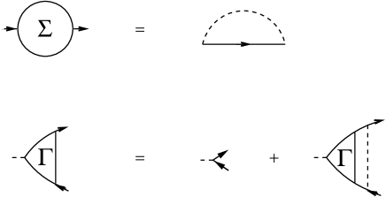
Figure 1: Conserving approximation for the self energy $\Sigma$ and the vertex function ${\bm{\Gamma}}$. Directed solid lines denote the Green function $G$, and dashed lines denote the effective potential $V$.

It is convenient to define a scalar vertex function $\gamma$ by ${\bm{\Gamma}}({\bm{p}};i\omega,i\omega^{\prime})=i({\bm{p}}/m)\,\gamma({\bm{p}});i\omega,i\omega^{\prime})$. $\gamma$ then obeys

$$\gamma_{\sigma}({\bm{p}};i\omega,i\omega-i\Omega) = 1+\frac{T}{V}\sum_{{\bm{k}},i\Omega^{\prime}}\sum_{\sigma^{\prime}}\,V_{\sigma\sigma^{\prime}}({\bm{p}}-{\bm{k}},i\Omega^{\prime})$$ (71)

$$\hskip-80.0pt\times\frac{{\bm{p}}\cdot{\bm{k}}}{{\bm{p}}^{2}}\,G_{\sigma^{\prime}}({\bm{k}},i\omega+i\Omega^{\prime})\,G_{\sigma^{\prime}}({\bm{k}},i\omega-i\Omega+i\Omega^{\prime})$$

$$\hskip-40.0pt\times\gamma_{\sigma^{\prime}}({\bm{k}};i\omega-i\Omega^{\prime},i\omega-i\Omega-i\Omega^{\prime})\ .$$

The polarization and conductivity tensors are diagonal, $\sigma_{ij}(i\Omega)=\delta_{ij}\,\sigma(i\Omega)$, and the sum over Matsubara frequencies in Eq. (69) can be transformed into an integral along the real axis. In the limit of low temperature, the imaginary part of the self energy goes to zero, and the real part just renormalizes the Fermi energy. The relevant limit is thus the one of a vanishing self energy, and in this limit the leading contributions to the integral come from terms where the frequency arguments of the two Green functions lie on different sides of the real axis. In the static limit, the Kubo formula for the conductivity $\sigma=\lim_{\Omega\to 0}{\text{Re}}\,\sigma(i\Omega\to\Omega+i0)$, thus becomes

$$\sigma = \frac{e^{2}}{3\pi m^{2}}\int_{-\infty}^{\infty}\frac{d\epsilon}{4T}\frac{1}{\cosh^{2}(\epsilon/2T)}\frac{1}{V}\sum_{{\bm{p}}}{\bm{p}}^{2}$$ (72)

$$\times\sum_{\sigma}|{\cal G}_{\sigma}({\bm{p}},\epsilon+i0)|^{2}\gamma_{\sigma}({\bm{p}};\epsilon+i0,\epsilon-i0)\ .\qquad$$

The pole of the Green function ensures that the dominant contribution to the momentum integral comes from the momenta that obey $\xi_{\sigma}({\bm{p}})=\epsilon$. Furthermore, since $\epsilon$ scales as $T$, for the leading $T$-dependence we can neglect all $\epsilon$-dependencies that do not occur in the form $\epsilon/T$. Equation (72) then reduces to Eq. (9a), with the relaxation rate $\varphi_{0}$ the solution of

$$\varphi_{0}^{\sigma}(\epsilon)\,\Gamma_{0}^{\sigma}(\epsilon)=1-\int du\sum_{\sigma^{\prime}}K^{\sigma\sigma^{\prime}}(\epsilon,u)\,\varphi_{0}^{\sigma^{\prime}}(u)$$ (73)

with $K$ as defined in Sec. II.2 and $\Gamma_{0}$ from Eq. (15). Here we have used the fact that the Green functions in Eq. (71) pin the wave vectors ${\bm{k}}$ and ${\bm{p}}$ to energy shells at distances $\epsilon\approx 0$ and $\epsilon+u\approx u$, respectively, from the Fermi surface, see Eq. (66). As a result, the factor ${\bm{p}}\cdot{\bm{k}}/{\bm{p}}^{2}$ in the integrand of Eq. (71) effectively becomes

$$\frac{{\bm{p}}\cdot{\bm{k}}}{{\bm{p}}^{2}}=1-\frac{{\bm{p}}\cdot({\bm{p}}-{\bm{k}})}{{\bm{p}}^{2}}\to 1-\frac{1}{2{\bm{p}}^{2}}({\bm{p}}-{\bm{k}})^{2}+\frac{mu}{{\bm{p}}^{2}}\ .$$ (74)

The second term on the far right-hand side is what is often called the “backscattering factor” in transport theory. It gives rise to the kernel $K_{2}$. The last term gives rise to the kernel $K_{3}$. $K_{1}$, the second contribution to $K_{3}$, and $K_{4}$ arise from the spin dependence of the density of states.

Equation (73) has the structure of the kinetic equation discussed in Ref. Bharadwaj et al., 2014. It can obviously be rewritten in the form of Eq. (11a). Note that Ref. Bharadwaj et al., 2014 ignored $K_{4}$ and the first contribution to $K_{3}$, an approximation that cannot be justfied a priori.K (34)

The equation for the relaxation function $\varphi_{1}$ is obtained by the same procedure, with the number current ${\bm{p}}/m$ in Eqs. (69) and (70) replaced by the heat current ${\bm{p}}\,\xi_{\sigma}({\bm{p}})/m$. This leads to Eq. (73) with the $1$ on the right-hand side replaced by $\epsilon$, and hence to Eq. (11b).

Appendix B Relaxation rates

The lowest eigenvalue of the collision operator calculated in Sec. III depends on the relaxation rates $\Gamma_{n}$, Eq. (15), averaged according to Eq. (23). In order to calculate the averages it is advantageous to do the $\epsilon$ integration first, making use of the integral

$$\frac{1}{T}\int d\epsilon\,w(\epsilon)\,f_{0}(x\mp\epsilon/T)=\frac{-1}{e^{x}-1}+\frac{x\,e^{x}}{(e^{x}-1)^{2}}$$ (75)

which is independent of the sign in the argument of the Fermi function $f_{0}$. We obtain

$$\langle\Gamma_{0}\rangle_{w_{\sigma}} = {\tilde{g}}_{0}(T_{\text{min}}+T)e^{-T_{\text{min}}/T}\ ,$$ (76a)

$$\langle\Gamma_{2}\rangle_{w_{\sigma}} = \frac{{\tilde{g}}_{0}}{1-4T_{0}/T_{1}}\left[-2\left(\frac{T_{\text{min}}^{2}}{T_{1}}+2\,\frac{T_{\text{min}}T}{T_{1}}+2\,\frac{T^{2}}{T_{1}}\right)\right.$$ (76b)

$$\hskip 35.0pt\left.+\frac{4T_{0}}{T_{1}}\left(T_{\text{min}}+T\right)\right]\,e^{-T_{\text{min}}/T}\ ,$$

$$\langle\Gamma_{4}\rangle_{w_{\sigma}} = \frac{2{\tilde{g}}_{0}\,T_{0}/\lambda}{1-4T_{0}/T_{1}}\left(\frac{T_{\text{min}}^{2}}{T_{1}}+2\,\frac{T_{\text{min}}T}{T_{1}}+2\,\frac{T^{2}}{T_{1}}\right)$$ (76c)

$$\hskip 80.0pt\times\,e^{-T_{\text{min}}/T}$$

Here ${\tilde{g}}_{0}=g_{0}8k_{\text{F}}^{+}k_{\text{F}}^{-}/k_{\text{F}}^{2}\nu$ with $\nu$ from Eq. (20c). The averages of $\Gamma_{1}$ and $\Gamma_{3}$ vanish by symmetry. Also useful is the average

$$\langle\epsilon\,\Gamma_{3}\rangle_{w_{\sigma}}={\tilde{g}}_{0}\left(\frac{4}{T_{1}}-\frac{1}{\lambda}\right)T_{0}^{3}\sqrt{\frac{T_{0}}{T_{1}}}\left[1+O(T_{0}/T_{1})\right]e^{-T_{\text{min}}/T}\ .$$ (77)

Appendix C Properties of the zero eigenvector

In this appendix we determine the overlap of the zero eigenvector $|e_{0}\rangle$ with $|\epsilon\rangle$ to lowest order in $\beta\sim\sqrt{T_{0}/T_{1}}$. In order to prove Eqs. (41c) and (43b) it is advantageous to rewrite the eigenproblem (35) by expanding the collision operator strictly in powers of $\beta\sim\sqrt{T_{0}/T_{1}}$. We define a collision operator

$$\tilde{\Lambda}_{0}^{\sigma}(\epsilon)=\int du\sum_{\sigma^{\prime}}\left[{\tilde{K}}_{0}^{\sigma\sigma^{\prime}}(\epsilon,u)\,R_{\epsilon\to u}^{\sigma\to\sigma^{\prime}}-{\tilde{K}}_{0}^{\sigma\sigma^{\prime}}(\epsilon,u)\right]\ .$$ (78a)

in terms of a kernel

$${\tilde{K}}_{0}^{\sigma\sigma^{\prime}}(\epsilon,u)=(N_{\text{F}}/N_{\text{F}}^{\sigma^{\prime}})K_{0}^{\sigma\sigma^{\prime}}(\epsilon,u)\ ,$$ (78b)

with $K_{0}$ from Eq. (16a). Similarly, we define

$$\tilde{\Lambda}_{1}^{\sigma}(\epsilon)=-2\left(\frac{T_{0}}{T_{1}}\right)^{1/2}\sigma\,\tilde{\Lambda}_{0}^{\sigma}(\epsilon)$$ (79a)

and

$$\tilde{\Lambda}_{2}^{\sigma}(\epsilon) = \int du\sum_{\sigma^{\prime}}{\tilde{K}}_{2}^{\sigma\sigma^{\prime}}(\epsilon,u)\,R_{\epsilon\to u}^{\sigma\to\sigma^{\prime}}+2\,\frac{T_{0}}{T_{1}}\,\tilde{\Lambda}_{0}^{\sigma}(\epsilon)$$

(79b)

$$\tilde{\Lambda}_{3}^{\sigma}(\epsilon) = \int du\sum_{\sigma^{\prime}}{\tilde{K}}_{3}^{\sigma\sigma^{\prime}}(\epsilon,u)\,R_{\epsilon\to u}^{\sigma\to\sigma^{\prime}}$$ (79c)

$$\hskip 50.0pt-4\left(\frac{T_{0}}{T_{1}}\right)^{3/2}\sigma\,\tilde{\Lambda}_{0}^{\sigma}(\epsilon)$$

where

$${\tilde{K}}_{2}^{\sigma\sigma^{\prime}}(\epsilon,u) = -2\left(\frac{|u-\epsilon|}{T_{1}}-\frac{T_{0}}{T_{1}}\right){\tilde{K}}_{0}^{\sigma\sigma^{\prime}}(\epsilon,u)$$ (80a)

$${\tilde{K}}_{3}^{\sigma\sigma^{\prime}}(\epsilon,u) = \left(\frac{T_{0}}{T_{1}}\right)^{1/2}\left(\frac{u-\epsilon}{\lambda}+4\,\frac{|u-\epsilon|}{T_{1}}\,\sigma-4\,\frac{T_{0}}{T_{1}}\,\sigma\right)$$ (80b)

$$\hskip 80.0pt\times{\tilde{K}}_{0}^{\sigma\sigma^{\prime}}(\epsilon,u)$$

The right eigenproblem (35) can then be rewritten as

$$\tilde{\Lambda}^{\sigma}(\epsilon)\,{\tilde{e}}_{0}^{\sigma}(\epsilon)=\mu_{0}\,{\tilde{e}}_{0}^{\sigma}(\epsilon)\,N_{\text{F}}/N_{\text{F}}^{\sigma}\ .$$ (81a)

where

$$\tilde{\Lambda}=\tilde{\Lambda}_{0}+\tilde{\Lambda}_{1}+\tilde{\Lambda}_{2}+\tilde{\Lambda}_{3}+O(\beta^{4})$$ (81b)

and

$${\tilde{e}}_{0}^{\sigma}(\epsilon)=(N_{\text{F}}^{\sigma}/N_{\text{F}})\,e^{\sigma}(\epsilon)\ .$$ (81c)

We further define a weight function

$${\tilde{w}}_{\sigma}(\epsilon)=\frac{1}{2}\,w(\epsilon)$$ (82a)

with $$w(\epsilon)$$ from Eq. (10a) and an associated scalar product

$$(\psi|\varphi)=\int d\epsilon\sum_{\sigma}{\tilde{w}}_{\sigma}(\epsilon)\,\psi^{\sigma}(\epsilon)\,\varphi^{\sigma}(\epsilon)$$ (82b)

in analogy to Eq. (22).

The advantage of this formulation is that various functions associated with $\tilde{\Lambda}_{0}$ have simple symmetry properties. For instance, the relaxation rates

$$\tilde{\Gamma}_{n}^{\sigma}(\epsilon)=\int du\sum_{\sigma^{\prime}}{\tilde{K}}_{n}^{\sigma\sigma^{\prime}}(\epsilon,u)\qquad(n=0,2)$$ (83a)

defined in analogy to Eq. (15) obey

$$\tilde{\Gamma}_{n}^{-}(-\epsilon)=\tilde{\Gamma}_{n}^{+}(\epsilon)\qquad(n=0,2)$$ (83b)

Similarly, the function ${\tilde{h}}$ defined in analogy to Eq. (30),

$$\tilde{\Lambda}_{0}|{\tilde{h}}\rangle=-|\epsilon\rangle$$ (84a)

obeys

$${\tilde{h}}^{-}(-\epsilon)=-{\tilde{h}}^{+}(\epsilon)$$ (84b)

A disadvantage is the resulting adjoint properties: $\tilde{\Lambda}_{0}$ and $\tilde{\Lambda}_{2}$ are self-adjoint with respect to the scalar product defined in Eq. (82b), but $\tilde{\Lambda}_{1}$ and $\tilde{\Lambda}_{3}$ are neither self-adjoint nor skew-adjoint. For our current purposes, this is irrelevant, but the symmetry properties expressed in Eqs. (83b) and (84b) are crucial.

We now solve the eigenproblem order by order in $\beta$ as in Sec. III.1.2. The eigenvalues are the same, as they must be. For the eigenvectors we obtain

$$|{\tilde{e}}_{0}^{(1)}\rangle=0\ ,$$ (85)

This is consistent with Eq. (LABEL:eq:3.9b), as can be seen by using Eq. (81c). The equation for $|{\tilde{e}}_{0}^{(2)}\rangle$ reads

$$\tilde{\Lambda}_{0}|{\tilde{e}}_{0}^{(2)}\rangle=-|\tilde{\Gamma}_{2}\rangle+\langle\tilde{\Gamma}_{2}\rangle_{\tilde{w}}\,|1\rangle\ .$$ (86a)

By multiplying from the left with $$\langle{\tilde{h}}|$$ and using Eqs. (83b) and (84b) we find

$$\langle\epsilon|{\tilde{e}}_{0}^{(2)}\rangle=0\ .$$ (86b)

Using Eq. (81c) yields Eq. (41c).

At the next order, analogous arguments yield

$$\langle\epsilon|{\tilde{e}}^{(3)}\rangle=\frac{-1}{\lambda}\left(\frac{T_{0}}{T_{1}}\right)^{1/2}\langle\epsilon|\epsilon\rangle\ .$$ (87)

Here we have used the fact that $\mu_{0}^{(2)}$ is exponentially small and can be neglected. The lowest component of $|e_{0}\rangle$ that has a nonzero overlap with $|\epsilon\rangle$ is thus $|e_{0}^{(3)}\rangle$, and to leading order $\langle\epsilon|e_{0}^{(3)}\rangle=\langle\epsilon|{\tilde{e}}_{0}^{(3)}\rangle$. We thus have

$$\langle\epsilon|e_{0}\rangle = -\left(\frac{T_{0}}{T_{1}}\right)^{1/2}\frac{1}{\lambda}\,\langle\epsilon|\epsilon\rangle\ ,$$ (88a)

$$\langle e_{0}|\epsilon\rangle = \left(\frac{T_{0}}{T_{1}}\right)^{1/2}\frac{1}{\lambda}\,\langle\epsilon|\epsilon\rangle\ .$$ (88b)

Note that the left and right eigenvectors are equal and opposite since $\Lambda_{3}$ (as opposed to $\tilde{\Lambda}_{3}$) is skew-adjoint. This is the result we have used in Eqs. (43).

References

- Bloch (1930) F. Bloch, Z. Phys. 59, 208 (1930).
- Ziman (1960) J. M. Ziman, Electrons and Phonons (Clarendon Press, Oxford, 1960).
- Yamada and Takada (1974) H. Yamada and S. Takada, Prog. Theor. Phys. 52, 1077 (1974).
- Ueda (1977) K. Ueda, J. Phys. Soc. Japan 43, 1497 (1977).
- Belitz et al. (2006) D. Belitz, T. R. Kirkpatrick, and A. Rosch, Phys. Rev. B 74, 024409 (2006), A description in terms of quasiparticles that simplifies the calculation of the transport properties is given in Refs. Kirkpatrick et al., 2008a and Kirkpatrick et al., 2008b.
- Ueda and Moriya (1975) K. Ueda and T. Moriya, J. Phys. Soc. Jpn. 39, 605 (1975).
- Bharadwaj et al. (2014) S. Bharadwaj, D. Belitz, and T. R. Kirkpatrick, Phys. Rev. B 89, 134401 (2014).
- Mahan (2000) G. D. Mahan, Many-Particle Physics (Kluwer, New York, 2000), 3rd ed.
- Amarel et al. (2020) J. Amarel, D. Belitz, and T. R. Kirkpatrick (2020), arXiv:2001.01148.
- (10) J. Amarel, D. Belitz, and T. R. Kirkpatrick, preceding paper (Paper I).
- (11) We consider a purely quadratic magnon dispersion relation for simplicity. Higher powers of in will lead to additional kernels that contribute to the collision operator in Sec. II. These kernels are of higher order in our power-counting scheme and can easily be taken into account, if desirable, within the framework of our solution scheme.
- Kubo (1957) R. Kubo, J. Phys. Soc. Jpn. 12, 570 (1957).
- K (34) An approximation in Ref. Bharadwaj et al., 2014 amounted to neglecting and the first term in . Our calculation will show that the contributions of these terms to the leading behavior of the transport coefficients cancel, which justifies this approximation a posteriori.
- (14) is proportional to the magnetization coefficient in Ref. Bharadwaj et al., 2014, or to the ferromagnon amplitude in Eq. (A.8a) of Paper I.
- Dorfman et al. (2021) J. R. Dorfman, H. van Beijeren, and T. R. Kirkpatrick, Contemporary Kinetic Theory of Matter (Cambridge University Press, to be published, 2021).
- (16) In order to avoid cumbersome notation we always denote right eigenvectors by and left eigenvectors by . It is important to remember that these two vectors represent different functions. In particular, for a given function . A more precise, if more complicated, notation would be to denote the right eigenfunctions by , and the left ones by , in which case .
- Kadanoff and Baym (1962) L. P. Kadanoff and G. Baym, Quantum Statistical Mechanics (W.A. Benjamin, New York, 1962).
- Kirkpatrick et al. (2008a) T. R. Kirkpatrick, D. Belitz, and R. Saha, Phys. Rev. B 78, 094407 (2008a).
- Kirkpatrick et al. (2008b) T. R. Kirkpatrick, D. Belitz, and R. Saha, Phys. Rev. B 78, 094408 (2008b).