Quantum coherence as a signature of chaos

Abstract

We establish a rigorous connection between quantum coherence and quantum chaos by employing coherence measures originating from the resource theory framework as a diagnostic tool for quantum chaos. We quantify this connection at two different levels: quantum states and quantum channels. At the level of states, we show how several well-studied quantifiers of chaos are, in fact, quantum coherence measures in disguise (or closely related to them). We further this connection for all quantum coherence measures by using tools from majorization theory. Then, we numerically study the coherence of chaotic-vs-integrable eigenstates and find excellent agreement with random matrix theory in the bulk of the spectrum. At the level of channels, we show that the coherence-generating power (CGP) — a measure of how much coherence a dynamical process generates on average — emerges as a subpart of the out-of-time-ordered correlator (OTOC), a measure of information scrambling in many-body systems. Via numerical simulations of the (nonintegrable) transverse-field Ising model, we show that the OTOC and CGP capture quantum recurrences in quantitatively the same way. Moreover, using random matrix theory, we analytically characterize the OTOC-CGP connection for the Haar and Gaussian ensembles. In closing, we remark on how our coherence-based signatures of chaos relate to other diagnostics, namely the Loschmidt echo, OTOC, and the Spectral Form Factor.

I Introduction

Quantum coherence and quantum entanglement are arguably the two cardinal attributes of quantum theory, originating from the superposition principle and the tensor product structure (TPS), respectively Nielsen and Chuang (2010); Streltsov et al. (2017); Horodecki et al. (2009). While entanglement as a signature of quantum chaos has been well-studied in both the few- and many-body case Wang et al. (2004); Vidmar and Rigol (2017); Kumari and Ghose (2019); Chaudhury et al. (2009); Neill et al. (2016), a rigorous connection between quantum coherence and quantum chaos still remains elusive. Here, we clarify in a quantitative way the role that quantum coherence plays in the study of chaotic quantum systems. Apart from the foundational role that the superposition principle plays in “everything quantum,” there are (at least) two distinct ways in which quantum coherence enters the study of quantum chaotic systems. The first, and perhaps the more conceptual one, is the Eigenstate Thermalization Hypothesis (ETH) Srednicki (1994); Deutsch (1991); Rigol et al. (2008) and the diagonal ensemble associated with it. The notion of quantum coherence is a basis-dependent one and the diagonal ensemble reveals the Hamiltonian eigenbasis as the relevant physical basis, especially when studying thermalization, ergodicity, and other temporal characteristics. Moreover, an initial state’s overlap with sufficiently many energy-levels — which is related to coherence in the energy-eigenbasis — is a sufficient condition for equilibration (under some additional assumptions) Reimann (2008); Linden et al. (2009); Short (2011). Second, the out-of-time-ordered correlator (OTOC) Larkin and Ovchinnikov (1969); Kitaev (2015) a quantifier of quantum chaos  and information scrambling, is usually studied via the input of two local unitaries and grows when they start noncommuting as one of them spreads under the Heisenberg time evolution. The locality of the observables in the OTOC “probes” the entanglement structure and its growth Lashkari et al. (2013); Kitaev (2015). At the same time, it is natural to ask, what does the strength of the noncommutativity probe (without reference to any TPS)? We argue that this is precisely a measure of quantum coherence (more specifically, the incompatibility of the bases associated to the unitaries Styliaris and Zanardi (2019)). For example, given two (non-degenerate) observables $A,B$ and the associated eigenbases $\mathbb{B}_{A},\mathbb{B}_{B}$, we can ask, how coherent are the eigenstates of $A$ when expressed in the (eigen)basis $\mathbb{B}_{B}$. Clearly, if $\left[A,B\right]=0$ then the eigenstates of $A$ are incoherent in $\mathbb{B}_{B}$. On the other hand, if $\mathbb{B}_{A}$ and $\mathbb{B}_{B}$ are mutually unbiased, then the eigenstates of $A$ are maximally coherent in $\mathbb{B}_{B}$, and various measures of incompatibility are maximized Styliaris and Zanardi (2019). Following this intuition, we will show that the OTOC is intimately related to a measure of incompatibility called the coherence-generating power (CGP), as exemplified by our 3.

Quantifying chaos.— Signatures of quantum chaos can be broadly classified into three categories: (i) spectral properties, such as level-spacing distribution Bohigas et al. (1984); Haake (2010), level number variance Guhr et al. (1998), etc., (ii) eigenstate structure, such as eigenstate entanglement (defined as the average entanglement entropy over all eigenstates) and the associated area and volume laws Eisert et al. (2010), and (iii) dynamical quantities such as Loschmidt echo Peres (1984); Jalabert and Pastawski (2001); Goussev et al. (2012); Gorin et al. (2006), entangling power Zanardi et al. (2000); Zanardi (2001); Wang et al. (2004); Scott and Caves (2003); Lakshminarayan (2001), quantum discord Madhok et al. (2015), OTOCs, etc. (see also Ref. Haake (2010) for other examples), which, in general are a property of both the eigenvalues and eigenvectors of the Hamiltonian. In this paper, we connect quantum chaos and quantum coherence in the sense of (ii) and (iii), by examining the coherence structure of chaotic-vs-integrable eigenstates, and by studying the coherence-generating power of chaotic dynamics.

Outline.—  This paper is organized as follows. In Section II, we review the resource theory of quantum coherence and the coherence measures that will be used throughout this paper. In Section III.1, we discuss connections between coherence measures and delocalization measures, first via examples, and then via the mathematical formalism of majorization. We also discuss the connection between coherence and entanglement and how their interplay affects coherence measures’ ability to diagnose quantum chaos. In Section III.2, we numerically examine the coherence structure of integrable-vs-chaotic eigenstates and introduce new tools inspired from majorization theory to study quantum chaos. In Section IV, we establish the connection between OTOC and CGP and, in particular, show how the CGP emerges as a subpart of the OTOC. Then, in Section IV.2, using tools from random matrix theory, we analytically perform averages over the CGP of random Hamiltonians and unveil a connection between CGP and the spectral form factor. We also study the short-time growth of the CGP and remark on its connection with quantum fluctuations and the resource theory of incompatibility. Furthermore, in Section IV.3, we numerically vindicate our OTOC-CGP connection by studying the integrable and chaotic regimes in a transverse-field Ising model. Finally, in Section V, we make some closing remarks and discuss our results. Our main results are stated as Theorems and all proofs can be found in the Appendix A3.

II Preliminaries.

Resource theory of quantum coherence.— Despite the fundamental role that quantum coherence plays in quantum theory, a rigorous quantification of coherence as a physical resource was only initiated in recent years Baumgratz et al. (2014); Aberg (2006); Streltsov et al. (2017). We briefly review the resource theory of coherence and the quantification tools it provides. Let $\mathcal{H}\cong\mathbb{C}^{d}$ be the Hilbert space associated to a $d$-dimensional quantum system and $S(\mathcal{H})$ the set of all quantum states. Quantum coherence of states is quantified with respect to a preferred orthonormal basis for the Hilbert space, $\mathbb{B}=\{|j\rangle\}_{j=1}^{d}$. All states that are diagonal in the basis $\mathbb{B}$ are deemed incoherent (that is, devoid of any resource) while others coherent. That is, incoherent states have the form, $\rho=\sum\nolimits_{j=1}^{d}p_{j}\Pi_{j}$, where $\Pi_{j}\equiv|j\rangle\langle j|$ is the rank-$1$ projector associated to the basis state $|j\rangle$ and $p_{j}\geq 0,\sum\nolimits_{j=1}^{d}p_{j}=1$ is a probability distribution. The collection of all incoherent states forms a convex set, $\mathcal{I}_{\mathbb{B}}$ (usually called the “free states” of the resource theory) . A common quantifier of the amount of resource in a state $\sigma$ is to measure its (minimum) distance from the set $\mathcal{I}_{\mathbb{B}}$, using appropriately chosen distance measures, say $\mathcal{R}_{\mathbf{d}}(\sigma)\coloneqq\min_{\delta\in\mathcal{I}_{\mathbb{B}}}\mathbf{d}(\sigma,\delta)$. where $\mathbf{d}(\cdot,\cdot)$ is a distance measure on the state space and $\mathcal{R}_{\mathtt{d}}$ its associated resource quantifier (usually called the “resource measures” of the resource theory). The coherence quantifiers that we will be working with in this paper are the $l_{2}$-norm of coherence  (hereafter $2$-coherence) and the relative entropy of coherence, defined as Baumgratz et al. (2014),

$$\mathtt{c}^{(\text{2})}_{\mathbb{B}}(\rho)\coloneqq\min_{\sigma\in\mathcal{I}_{\mathbb{B}}}\left\|\rho-\sigma\right\|_{l_{2}}^{2}=\left\|\rho-\mathcal{D}_{\mathbb{B}}(\rho)\right\|_{l_{2}}^{2},$$ (1)

$$\mathtt{c}^{(\text{rel})}_{\mathbb{B}}(\rho)\coloneqq\min_{\sigma\in\mathcal{I}_{\mathbb{B}}}S^{(\text{rel})}(\rho||\sigma)=S(\mathcal{D}_{\mathbb{B}}(\rho))-S(\rho),$$ (2)

where, $\mathcal{D}_{\mathbb{B}}(X)\coloneqq\sum_{j=1}^{d}\Pi_{j}X\Pi_{j}$ is the dephasing superoperator, $S^{(\text{rel})}(\rho||\sigma)$ is the quantum relative entropy, and $S(\rho)$ is the von Neumann entropy Baumgratz et al. (2014). The $2$-coherence  has been identified as the escape probability, a key figure of merit for few- and many-body localization Styliaris et al. (2019), while the relative entropy of coherence has several operational interpretations, prominent amongst which are its role as the distillable coherence Winter and Yang (2016) and as a measure of deviations from thermal equilibrium Rodríguez-Rosario et al. (2013).

A final but key ingredient of quantum resource theories are the so-called “free operations,” transformations that do not generate any resource, but may consume it. For the resource theory of coherence, we will focus on the class of incoherent operations (IO): completely-positive (CP) maps such that there exists at least one Kraus representation which satisfies $K_{j}\rho K_{j}^{\dagger}/\operatorname{Tr}\left(K_{j}\rho K_{j}^{\dagger}\right)\in\mathcal{I}_{\mathbb{B}}\leavevmode\nobreak\ \leavevmode\nobreak\ \forall\rho\in\mathcal{I}_{\mathbb{B}},\leavevmode\nobreak\ \leavevmode\nobreak\ \forall j$ . Resource measures that are non-increasing under the action of free operations are called resource monotones.

III At the level of states

III.1 Why study quantum coherence?

The sudden delocalization of chaotic systems following a quench has been well-studied for both classical and quantum systems, see Refs. D’Alessio et al. (2016); Borgonovi et al. (2016) and the references therein. Various quantifiers of this delocalization have been introduced in the quantum chaos literature to characterize integrable and chaotic quantum systems. Here, we argue that many of these delocalization measures are nothing but quantum coherence measures in disguise. We argue this in two ways: first, we consider some paradigmatic measures of delocalization such as Shannon entropy, participation ratio, etc., Kota (2014) and connect them with measures of quantum coherence studied in the resource theories framework. Moreover, this also reveals that the notion of delocalization in the available phase space, energy space, etc., is precisely the notion of quantum coherence in an appropriate basis. Second, we show that the notion of when one state is more delocalized than the other (and measures to quantify them) is captured in a very general way by the mathematical formalism of majorization. This further allows us to make a precise connection to the resource theory of coherence since state transformation under incoherent operations is completely characterized in terms of majorization. Finally, using the majorization result from the resource theoretic framework of coherence, we argue that quantum coherence measures capture precisely what delocalization measures set out to quantify: how “localized” or “uniformly spread” a quantum state is across a basis. Along the way we also remark on coherence measures’ ability to probe entanglement measures, which have long been used as quantifiers of chaos.

Connection with delocalization measures.—  Let us start with a simple example: Given a state $|\psi\rangle$ expressed in some basis $\mathbb{B}=\{|j\rangle\}$, $|\psi\rangle=\sum\nolimits_{j=1}^{d}c_{j}|j\rangle$, one can consider various ways to quantify how uniformly spread the probability distribution generated from $\{\left|c_{j}\right|^{2}\}$ is. For instance, an incoherent state $|j\rangle$ corresponds to the (extremely) nonuniform probability distribution $\mathbf{p}_{|j\rangle}=\{1,0,\cdots,0\}$, that is, it is the most “localized” state; while a highly coherent state  of the form $|\psi\rangle=\frac{1}{\sqrt{d}}\sum\limits_{j=1}^{d}e^{-i\theta_{j}}|j\rangle$ corresponds to the uniform probability distribution $\mathbf{p}_{|\psi\rangle}=\{\frac{1}{d},\frac{1}{d},\cdots,\frac{1}{d}\}$, that is, it is maximally “delocalized”. Therefore, if we quantify the uniformity of the associated probability distributions by evaluating, for example, their Shannon entropy, we see that the incoherent state corresponds to the minimum entropy $S(\{\left|c_{\alpha}\right|^{2}\})=0$, while the highly coherent state maximizes the Shannon entropy, $S(\{\left|c_{\alpha}\right|^{2}\})=\log\left(d\right)$. This uniformity is precisely what coherence measures and delocalization measures quantify.

We now discuss some examples where there is a precise connection between them. We consider the same notation as above, a pure state $|\psi\rangle$, a basis $\mathbb{B}=\{|j\rangle\}$, and $\{p_{j}\}_{j=1}^{d}$, where $p_{j}\equiv\left|\left\langle k|\psi\right\rangle\right|^{2}$ is the associated probability distribution.

1. The Shannon entropy (also known as the informational entropy in the quantum chaos literature) of the probability distribution $\{p_{j}\}_{j=1}^{d}$ has been used as a measure of delocalization Kota (2014); D’Alessio et al. (2016); Borgonovi et al. (2016). We note that for pure states, this is equal to the relative entropy of coherence. That is,

$$\mathtt{c}^{(\text{rel})}_{\mathbb{B}}(\rho)=S(\{p_{j}\})$$ (3)

This follows from the definition in Eq. 1 and the fact that the Shannon entropy of pure states is zero, that is, $S(|\psi\rangle\langle\psi|)=0$. It is worth noting that the Shannon entropy is the first Rényi entropy Rényi et al. (1961), a family of entropies which provide powerful connections with majorization theory and state transformation in resource theories Chitambar and Gour (2019).

2. The second participation ratio (also known as the number of principal components) Kota (2014); D’Alessio et al. (2016); Borgonovi et al. (2016), defined as

$$\mathrm{PR}_{2,\mathbb{B}}(|\psi\rangle)\coloneqq\sum_{j}|\langle j|\psi\rangle|^{4}.$$ (4)

Note that for pure states and any given basis $\mathbb{B}$, the $\mathrm{PR}_{2,\mathbb{B}}$ is equal to one minus the $2$-coherence, that is ,

$$\mathrm{PR}_{2,\mathbb{B}}(|\psi\rangle)=1-\mathtt{c}^{(2)}_{\mathbb{B}}(|\psi\rangle\langle\psi|).$$ (5)

Moreover, the negative logarithm of $\mathrm{PR}_{2}$ is equal to the second Rényi entropy Rényi et al. (1961) of the probability distribution $\{p_{j}\}$. And both the first and second Rényi entropies are measures of quantum coherence Streltsov et al. (2017).

3. We now review three quantities, the Loschmidt echo, the escape probability and the effective dimension, which find a multitude of applications in quantum chaos, thermalization, and localization. The Loschmidt echo is defined as the overlap between the initial state $\ket{\psi}$ and the state after time $t$ Peres (1984); Jalabert and Pastawski (2001); Gorin et al. (2006),

$$\mathcal{L}_{t}(|\psi\rangle)\coloneqq\left|\langle\psi|e^{-iHt}|\psi\rangle\right|^{2}.$$ (6)

The effective dimension of a quantum state is defined as its inverse purity Reimann (2008); Linden et al. (2009),

$$d^{\mathrm{eff}}(\rho)=\frac{1}{\mathrm{Tr}[\rho^{2}]},$$ (7)

which intuitively corresponds to the number of pure states that contribute to the (in general) mixed state $\rho$. In Refs. Reimann (2008); Linden et al. (2009), $d^{\mathrm{eff}}(\rho)$ was used to provide a sufficient condition for equilibration in closed quantum systems. And finally, we recall that the infinite-time average of a quantity $A$ is defined as

$$\overline{A}\coloneqq\lim_{T\rightarrow\infty}\frac{1}{T}\int\limits_{0}^{T}A(t)dt.$$ (8)

Infinite-time averaging connects these various quantities as follows (with $\rho=|\psi\rangle\langle\psi|$)

$$\overline{\mathcal{L}_{t}(|\psi\rangle)}=\textnormal{PR}_{2,\mathbb{B}_{\mathrm{H}}}(\rho)=\frac{1}{d^{\mathrm{eff}}(\overline{\rho})}=1-\mathcal{P}_{\psi},$$ (9)

where $\mathbb{B}_{\mathrm{H}}$ is the Hamiltonian eigenbasis and $\mathcal{P}_{\psi}:=1-\overline{\left|\left\langle\psi\left|e^{-iHt}\right|\psi\right\rangle\right|^{2}}$ is the escape probability of the state $|\psi\rangle$; which using Proposition 4 of Ref. Styliaris and Zanardi (2019) is also equal to the $2$-coherence in the Hamiltonian eigenbasis.

Note that, the proof of Proposition 4 in Ref. Styliaris and Zanardi (2019) can potentially reveal many more connections since there it was observed that the infinite time-average of the time evolution operator (for a non-degenerate Hamiltonian) $\mathcal{U}_{t}\coloneqq U(\cdot)U^{\dagger}$ is equivalent to dephasing in the Hamiltonian eigenbasis, that is, $\overline{\mathcal{U}_{t}}=\mathcal{D}_{\mathbb{B}_{\mathrm{H}}}$. The action of $\mathcal{D}_{\mathbb{B}_{\mathrm{H}}}$ reveals the “diagonal ensemble,” fundamental to the study of thermalization in closed quantum systems Rigol et al. (2008).

Arbitrary coherence measures and majorization.—  Given two vectors $\vec{v},\vec{w}\in\mathbb{R}^{n}$, we say that “$\vec{v}$ is majorized by $\vec{w}$,” (equivalently $\vec{w}$ majorizes $\vec{v}$) written as $\vec{v}\prec\vec{w}$, if Marshall et al. (2011)

$$\begin{aligned} \sum_{j=1}^{k}v_{[j]}&\leq\sum_{j=1}^{k}w_{[j]},\forall k=1,\cdots,n-1\\ \sum_{j=1}^{n}v_{[j]}&=\sum_{j=1}^{n}w_{[j]},\end{aligned}$$ (10)

where $v_{[j]}$ is the $j$th element of $\vec{v}$ when sorted in a nonincreasing order. Majorization induces a preorder  on the vectors in $\mathbb{R}^{n}$ and it is natural to ask what functions preserve this preorder? All functions $f:\mathbb{R}^{n}\rightarrow\mathbb{R}$ such that $\vec{v}\prec\vec{w}\implies f(\vec{v})\leq f(\vec{w})$ are called Schur-convex (equivalently, Schur-concave if $\vec{v}\prec\vec{w}\implies f(\vec{v})\geq f(\vec{w})$). Many functionals employed in the study of quantum chaos like Shannon entropy, the family of Rényi entropies, and others, are an example of Schur-concave functions that preserve the ordering imposed from majorization. Using a theorem of Hardy-Littlewood-Polya Marshall et al. (2011), we have the following

$$\vec{v}\prec\vec{w}\iff\sum_{j=1}^{n}g\left(v_{j}\right)\leq\sum_{j=1}^{n}g\left(w_{j}\right),$$ (11)

for all continuous convex functions $g:\mathbb{R}\rightarrow\mathbb{R}$.

That is, studying majorization is equivalent to studying the ordering induced from all continuous convex functions obeying an ordering. It is in this specific sense that majorization allows us to go beyond any specific quantum coherence measure and allows us to discuss the behavior of all coherence measures.

To make the connection to quantum coherence, we note that given two states $\rho,\sigma$ and a coherence measure $\mathtt{c}_{\mathbb{B}}(\cdot)$, if $\mathtt{c}_{\mathbb{B}}(\rho)>\mathtt{c}_{\mathbb{B}}(\sigma)$ then $\sigma$ cannot be transformed into $\rho$ via incoherent operations (since IO can only nonincrease the amount of coherence in a state). On the other hand, $\mathtt{c}_{\mathbb{B}}(\rho)\leq\mathtt{c}_{\mathbb{B}}(\sigma)$ provides a necessary (but not sufficient) condition on the state transformation $\sigma\mapsto\rho$ using IO. A necessary and sufficient condition was obtained in Ref. Du et al. (2015) in terms of majorization (the theorem has been rephrased for simplicity). In the following, $\mathcal{D}_{\mathbb{B}}$ is the dephasing superoperator in the basis $\mathbb{B}$; and the notion of matrix majorization has been used, with $A\prec B\iff\mathrm{spec}(A)\prec\mathrm{spec}(B)$, where $\mathrm{spec}(A)$ is the vector of eigenvalues of $A$.

Theorem 1 (Du et al. (2015)).

A quantum state $|\psi\rangle$ can be transformed to another state $|\phi\rangle$ via incoherent operations if and only if $\mathcal{D}_{\mathbb{B}}\left(|\psi\rangle\langle\psi|\right)\prec\mathcal{D}_{\mathbb{B}}\left(|\phi\rangle\langle\phi|\right)$.

Remark: First, note that $\mathcal{D}_{\mathbb{B}}\left(|\psi\rangle\langle\psi|\right)\equiv\mathbf{p}_{\psi}$ is isomorphic to the probability vector obtained from the state $|\psi\rangle$ expressed in the basis $\mathbb{B}$. Therefore, the condition $\mathcal{D}_{\mathbb{B}}\left(|\psi\rangle\langle\psi|\right)\prec\mathcal{D}_{\mathbb{B}}\left(|\phi\rangle\langle\phi|\right)=\mathbf{p}_{\psi}\prec\mathbf{p}_{\phi}$, that is, it is equivalent to the state $|\psi\rangle$ being more uniformly spread in the basis $\mathbb{B}$ than the state $|\phi\rangle$, in the sense of majorization. Now, since the majorization condition is equivalent  to transforming $|\psi\rangle\mapsto|\phi\rangle$ via an incoherent operation, the amount of coherence in $|\psi\rangle$ is greater than or equal to the amount of coherence in $|\phi\rangle$, for every quantum coherence measure. Formally, $\mathcal{R}_{c}\left(|\psi\rangle\langle\psi|\right)\geq\mathcal{R}_{c}\left(|\phi\rangle\langle\phi|\right)$, for every coherence monotone $\mathcal{R}_{c}:\mathcal{S}(\mathcal{H})\rightarrow\mathbb{R}_{0}^{+}$. Therefore, quantum coherence measures capture in a precise sense what traditional delocalization measures set out to quantify: how uniformly spread is a quantum state with respect to a basis $\mathbb{B}$; in fact, the above theorem quantitatively shows that these two notions are equivalent.

Having established a web of connections between several key quantities used in the study of quantum chaos and equilibration, we now discuss how quantum coherence measures can inherit their ability to diagnose quantum chaos from their interplay with entanglement measures.

(a)

(b)

Figure 1: Relative entropy of coherence for eigenstates of the Hamiltonian defined in Eq. 13 as a function of their energy, normalized with the GOE prediction using Eq. 14, $\left\langle\mathtt{c}^{(\text{rel})}_{\mathbb{B}}\right\rangle_{\mathrm{GOE}}\approx 10.49$. Results are reported for $L=15$ with $5$ spins up and $\omega=0$, $\epsilon_{\delta}=0.5$, $J_{xy}=1$, $J_{z}=0.5$. The plot markers $1,3,5,7$ correspond to the various choices of the defect site, with $\delta=1$ and $\delta=7$ corresponding to the integrable and chaotic limits, respectively. Figures (a) and (b) correspond to the two different bases, the site-basis and mean-field basis, respectively.

Coherence and its interplay with entanglement.— The study of quantum coherence per se, makes no reference to the locality (or TPS) of a quantum system. However, many-body systems are often endowed with a natural TPS and to study the interplay between coherence and entanglement, it is often convenient to choose incoherent states that are compatible with the TPS, namely, the incoherent states are also product states Streltsov et al. (2015); Chitambar and Hsieh (2016). Consider, for example, a two-qubit system, $\mathcal{H}\cong\mathbb{C}^{2}\otimes\mathbb{C}^{2}$, with an incoherent basis $\mathbb{B}=\{|00\rangle,|01\rangle,|10\rangle,|11\rangle\}$ that is also separable . Then, notice that any entangled state is automatically coherent, since $|\Psi_{AB}\rangle$ is entangled if and only if $|\Psi_{AB}\rangle\neq|\phi\rangle_{A}\otimes|\phi\rangle_{B}$ for any $|\phi\rangle_{A(B)}\in\mathcal{H}_{A(B)}$. Therefore, when expressed as a linear combination of the basis elements in $\mathbb{B}$, we note that, for every entangled state, $|\Psi_{AB}\rangle=\sum\nolimits_{j,k=0}^{1}c_{jk}|j\rangle_{A}|k\rangle_{B}$, we have at least two non-zero coefficients $c_{jk}$ — that is, they are coherent as well. Clearly, not every coherent state is entangled, for example, consider the state $|0\rangle\otimes|+\rangle$. This construction can be generalized to the (simplest) multipartite  case as follows: Let $\mathcal{H}\cong\mathcal{H}_{1}\otimes\mathcal{H}_{2}\otimes\cdots\mathcal{H}_{n}$ be a $n$-partite Hilbert space with $\mathcal{F}_{e}$ being the set of fully separable states (that is, they are convex combinations of states that factorize over any tensor factor) and $\mathcal{F}_{c}$ being the set of incoherent states that are also fully separable. Then, it is easy to see that $\mathcal{F}_{c}\subset\mathcal{F}_{e}$ (since the $\mathcal{F}_{c}$ is compatible with the TPS). As an immediate consequence, note that, if $\mathcal{R}(\cdot,\cdot):\mathcal{S}(\mathcal{H})\rightarrow\mathbb{R}_{0}^{+}$ is a contractive distance (under the associated free operations, that leave the set of free states invariant), then, one can define a “distance-based measure,” $\mathcal{R}_{\alpha}(\rho)\coloneqq\min_{\sigma\in\mathcal{F}_{\alpha}}\mathcal{R}(\rho,\sigma)$, where $\alpha=\{c,e\}$. Then, using the set inclusion of $\mathcal{F}_{c},\mathcal{F}_{e}$, we have, $\leavevmode\nobreak\ \leavevmode\nobreak\ \forall\rho,\mathcal{R}_{c}(\rho)\geq\mathcal{R}_{e}(\rho)$, that is, the amount of coherence is lower-bounded by the entanglement; or, the amount of coherence is an upper bound on the amount of entanglement .

In light of the above observation, it is worth noting that there is a semantical issue in calling these functionals delocalization measures since there is, per se, no locality in their definition. At this point, it is more appropriate to think of them as quantifying the coherence of a state in some basis, $\mathbb{B}$; in fact, their definition reveals that this is precisely what they do. To connect quantum coherence with entanglement in a quantitative way (apart from the bounds realized from the discussion above), as a first step, one needs to define a quantity that removes the basis-dependence of coherence (since entanglement is basis-independent), which can be obtained by optimizing over various choices of bases. Here, we prove one such result by minimizing the amount of coherence over all local bases: Given pure states in $\mathcal{H}\cong\mathcal{H}_{a}\otimes\mathcal{H}_{b}$, we have,

Theorem 2.

$$\min_{\mathbb{B}_{a},\mathbb{B}_{b}}\mathtt{c}^{(\text{2})}_{\mathbb{B}_{a}\otimes\mathbb{B}_{b}}(|\Psi\rangle\langle\Psi|)=1-\left\|\rho_{a}\right\|_{2}^{2}=:S_{\mathrm{lin}}(\rho_{a}),$$ (12)

where $\rho_{a}=\operatorname{Tr}_{b}\left(|\Psi\rangle\langle\Psi|\right)$ is the reduced density matrix and $S_{\mathrm{lin}}(\cdot)$ is the linear entropy, a quantifier of entanglement.

That is, by minimizing the amount of coherence over all local bases, we can (indirectly) compute a measure of entanglement. Another quantitative connection was obtained in Ref. Streltsov et al. (2018), where, by maximizing the amount of coherence over all bases, the amount of coherence in a state was connected with its purity. In summary, quantum coherence measures provide both upper bounds and in some cases precise connections with entanglement measures. Since entanglement measures have been widely used to detect quantum chaos, we now turn to studying quantum coherence in chaotic systems.

III.2 Coherence of many-body eigenstates: XXZ spin-chain with defect

(a)

(b)

Figure 2: $2$-coherence for eigenstates of the Hamiltonian defined in Eq. 13 as a function of their energy, normalized with the GOE prediction obtained numerically, $\left\langle\mathtt{c}^{(2)}_{\mathbb{B}}\right\rangle_{\mathrm{GOE}}\approx 0.9991$. Results are reported for $L=15$ with $5$ spins up and $\omega=0$, $\epsilon_{\delta}=0.5$, $J_{xy}=1$, $J_{z}=0.5$. The plot markers $1,3,5,7$ correspond to the various choices of the defect site, with $\delta=1$ and $\delta=7$ corresponding to the integrable and chaotic limits, respectively. Figures (a) and (b) correspond to the two different bases, the site-basis and mean-field basis, respectively.

The entanglement structure of excited states has been shown to be a successful diagnostic of quantum chaos Garrison and Grover (2018); Deutsch (2010); Huang (2019). Here, we numerically study the coherence structure of Hamiltonian eigenstates, using an open XXZ spin-chain with an onsite defect , described via a Hamiltonian of the form Santos (2004); Gubin and F. Santos (2012)

$$\begin{aligned} H&=\underbrace{\frac{1}{4}\sum\limits_{j=1}^{L-1}\left(J_{xy}\left(\sigma^{x}_{j}\sigma^{x}_{j+1}+\sigma^{y}_{j}\sigma^{y}_{j+1}\right)+J_{z}\sigma^{z}_{j}\sigma^{z}_{j+1}\right)}_{H_{\mathrm{XXZ}}}\\ &+\underbrace{\frac{1}{2}\left(\sum\limits_{j=1}^{L}\omega\sigma^{z}_{j}+\epsilon_{\delta}\sigma^{z}_{\delta}\right)}_{H_{z}},\end{aligned}$$ (13)

where $\delta\in\{1,2,\cdots,L\}$ is the label for the defect site. We set $\hbar=1$ and all sites have the same energy splitting, except the site $\delta$, which has a splitting of $\omega+\epsilon_{\delta}$ (the defect corresponds to a different value of the Zeeman splitting). We assume open boundary conditions and set the various parameters to the following values: $\omega=0,\epsilon_{\delta}=0.5,J_{xy}=1,J_{z}=0.5$; for a detailed discussion of the physics surrounding the choice of parameters and how this leads to the onset of chaos, see Sec. II of Ref. Santos (2004); Gubin and F. Santos (2012). It is easy to see that the total spin in $z$-direction is conserved, that is, $\left[H,\sigma^{z}_{\mathrm{total}}\right]$, where $\sigma_{\mathrm{total}}^{z}\equiv\sum\nolimits_{j=1}^{L}\sigma_{j}^{z}$. The Hamiltonian in Eq. 13 is integrable when the defect is on the edges of the chain, that is, $\delta=1$ or $L$, while it is non-integrable for the defect in the middle of the chain $\delta=\left\lfloor{L/2}\right\rfloor$ Santos (2004); Gubin and F. Santos (2012). One way to observe this transition to non-integrability is via the level-spacing distribution of the Hamiltonian, as studied in Ref. Santos (2004); Gubin and F. Santos (2012) and reproduced independently in Fig. 5. The level-spacing distribution transitions from a Poisson to a (universal) Wigner-Dyson form, a common signature of quantum chaos. Note that, in general, to obtain a Wigner-Dyson level-spacing distribution for chaotic systems, one needs to make sure that all the symmetries have been removed, that is, we are working in a specific symmetry sector of the system. For the system in Eq. 13, we consider the spin subspace corresponding to $\left\lfloor\frac{L}{3}\right\rfloor$ spins up; once we are in this subspace, there are no degeneracies in the Hamiltonian, see Refs. Santos (2004); Gubin and F. Santos (2012) for more details. Moreover, for the XXZ model with defect, Refs. Torres-Herrera and Santos (2014); Torres-Herrera et al. (2015); Torres-Herrera and Santos (2017) verified other signatures of quantum chaos such as local observables satisfying diagonal ETH D’Alessio et al. (2016); Borgonovi et al. (2016), and the long-time dynamics developing spectral correlations. Furthermore, in recent years, this model has also been employed in the study of many-body chaos Pandey et al. (2020), thermalization Brenes et al. (2020); Richter et al. (2020), and quantum transport Žnidarič (2020).

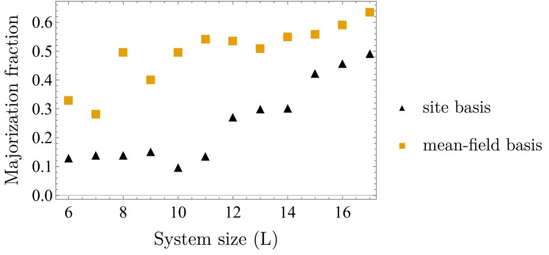
(a)

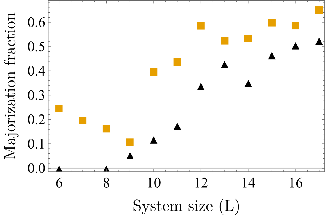
(b)

Figure 3: Fraction of integrable eigenstates that majorize chaotic eigenstates for the Hamiltonian defined in Eq. 13 system size $L$. Here, $\delta=1$ for integrable eigenstates, and $\delta=\lfloor{L/2}\rfloor$ for chaotic eigenstates. The plot markers correspond to the two different bases, the site-basis and mean-field basis, respectively. Figures (a) and (b) correspond to the full spectrum and 20% of eigenvectors in the middle of the spectrum, respectively.

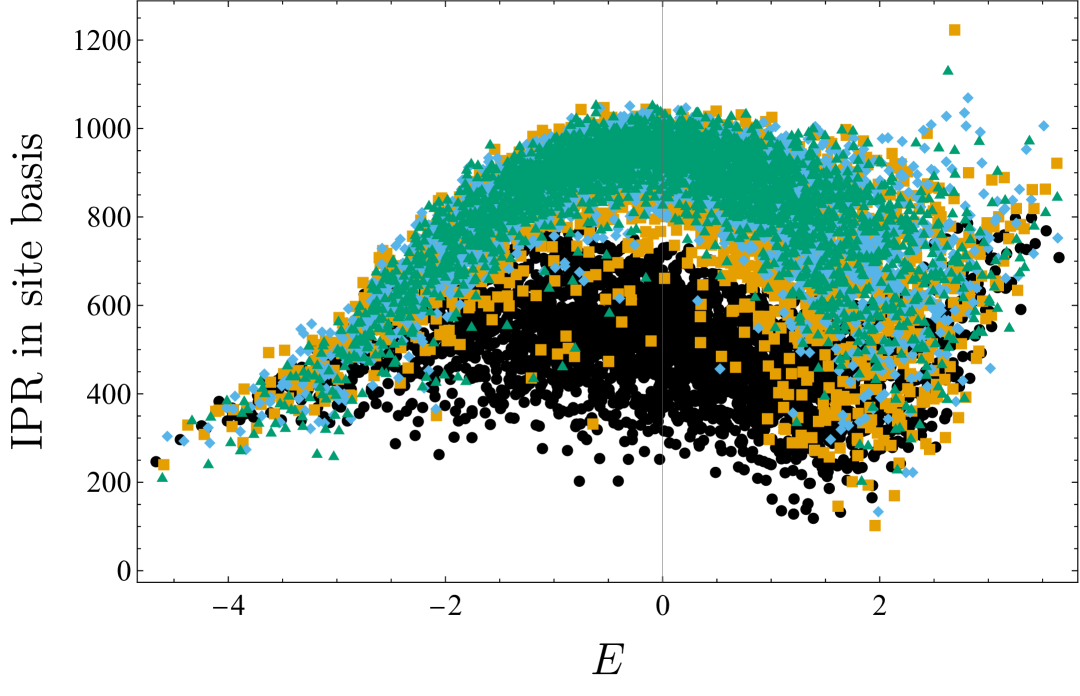
(a)

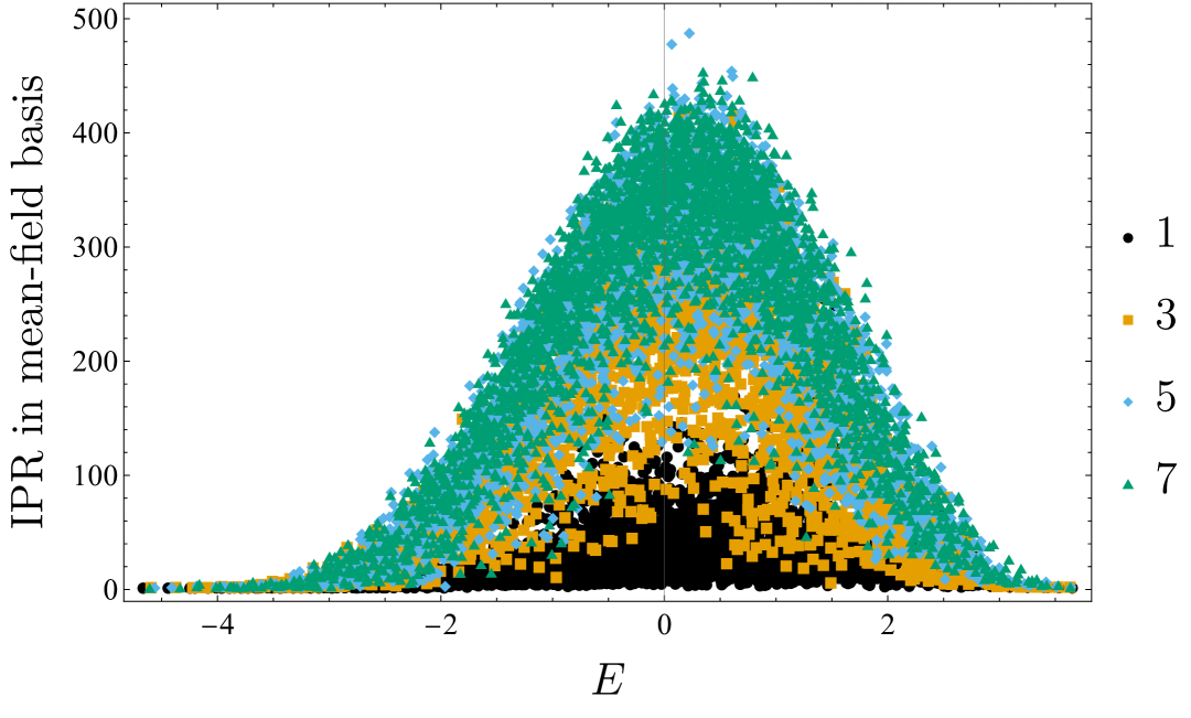
(b)

Figure 6: Inverse participation ratio for eigenstates of the Hamiltonian defined in Eq. 13 as a function of their energy. Results are reported for $L=15$ with $5$ spins up and $\omega=0,\epsilon_{\delta}=0.5,J_{xy}=1,J_{z}=0.5$. The plot markers $1,3,5,7$ correspond to the various choices of the defect site, with $\delta=1,7$ corresponding to the integrable and chaotic limits, respectively. Figures (a) and (b) correspond to the two different bases, the site-basis and the mean-field basis, respectively. Similar results were obtained for $L=18$ and $\delta=1,9$ in Ref. Gubin and F. Santos (2012) (but not for intermediate positions of the defect site).

In Ref. Santos and Rigol (2010), the participation ratio as an indicator of chaos was studied and results similar to Fig. 6 were obtained. Using the relative entropy of coherence, $2$-coherence, inverse participation ratio (IPR), and $1$-norm coherence, we study the onset of chaos, as the defect site is moved to the middle of the chain. We study coherence in two different bases, the “site basis” and the “mean-field basis”. The site basis is simply the local $\sigma^{z}$ basis at each site and coherence in this basis is a measure of how uniformly spread is the eigenstate with respect to the local subsystems. To define the mean-field basis, we start by expressing the total Hamiltonian as $H_{\mathrm{total}}=H_{0}+V$, where $H_{0}$ is the Hamiltonian of noninteracting particles (or, more generally, degrees of freedom) and $V$ the interaction between them Santos et al. (2012); Zelevinsky et al. (1996). The mean-field basis is then the eigenbasis of the “mean-field Hamiltonian,” $H_{0}$. This is, in fact, quite similar to the mean-field approach used in atomic and nuclear physics (and hence the terminology). It is immediately apparent that such a decomposition of the total Hamiltonian is not unique, however, in many physical scenarios, there is a natural choice of the mean-field basis. The intuition here is that as the interaction strength increases, the eigenstates of the total Hamiltonian will become more uniformly spread when expressed in the mean-field basis. Following Refs. Santos (2004); Gubin and F. Santos (2012), we take the mean-field Hamiltonian to be $J_{xy}\neq 0,\epsilon_{\delta}\neq 0,J_{z}=0$. Notice that this is not the same as the integrable limit above.

Random matrix theory.— Before going into the details of our numerical studies, let us briefly recall some key ideas from random matrix theory (RMT) and its predictions for quantum chaotic systems. First introduced by Wigner Wigner (1955, 1957, 1958) and later developed by Dyson Dyson (1962), RMT has been widely used to study complex systems and in particular, quantum chaotic systems (see Refs. D’Alessio et al. (2016); Borgonovi et al. (2016) for a pedagogical review). Many of the originally introduced measures (like level-spacing distribution) were purely spectral properties, but in recent years, there has been more interest in going beyond the spectral properties to understand the eigenstate structure of chaotic systems D’Alessio et al. (2016); Borgonovi et al. (2016). For instance, if quantum chaotic systems can be well-described by RMT, then their eigenstate properties are expected to resemble those of random vectors in the Hilbert space (namely, the eigenvectors of RMT Hamiltonians). However, this is not the complete picture. Many of the traditional Gaussian ensembles like the Gaussian Orthogonal Ensemble (GOE), Gaussian Unitary Ensemble (GUE), etc. are ensembles of many-body interactions and not $2$- and $3$-body interactions (reminiscent of physical Hamiltonians), and the properties of few-body Hamiltonians can be modelled more accurately by the use of the so-called embedded ensembles Kota (2014). Moreover, numerical studies have revealed that generically, only eigenstates in the middle of the spectrum correspond well to the (usual) RMT prediction (as will also be relevant for our numerical studies) Santos and Rigol (2010); Santos et al. (2012); Kota (2014).

We also note that using the connection between Shannon entropy and relative entropy of coherence as discussed in Section III.1, we can infer analytically the ensemble averaged relative entropy of coherence for GOE eigenstates (see Sec. 2.3.2 of Ref. Kota (2014))

$$\left\langle\mathtt{c}^{(\text{rel})}_{\mathbb{B}}\right\rangle_{\mathrm{GOE}}=\ln\left(0.48d\right)+O\left(\frac{1}{d}\right),$$ (14)

where $d$ is the Hilbert space dimension. Since GOE eigenvectors are (Haar) uniformly distributed, the basis $\mathbb{B}$ is a generic basis, that is, the estimate for the ensemble average holds true for any basis D’Alessio et al. (2016); Borgonovi et al. (2016). We use this analytical expression for normalizing the quantities studied in Figs. 2 and 1.

The Hamiltonian in Eq. 13 is real and symmetric and belongs to the Gaussian Orthogonal Ensemble (GOE) universality class. In Figs. 6, 2, 1 and 7, we study the aforementioned coherence measures normalized by the GOE prediction and find that, in the middle of the spectrum, the chaotic model does reproduce the GOE prediction; which is consistent with previously known results (that the eigenstates of systems with few-body interactions delocalize in the middle of the spectrum) Kota (2014); Santos (2004); Gubin and F. Santos (2012); Santos and Rigol (2010); Santos et al. (2012). Thus, this vindicates the various coherence measures as a signature of the transition to chaos.

What about other quantum coherence measures?— Apart from the specific quantum coherence measures studied above, what, if anything, can be said about an arbitrary coherence measures’ ability to probe quantum chaos in a similar way? To answer this question, we turn to the powerful mathematical formalism of majorization theory Marshall et al. (2011) as discussed in Section III.1. We numerically study the majorization condition in 1 for the integrable and chaotic eigenstates of the XXZ spin-chain in Eq. 13 and analyze the extent to which the induced preorder order holds true. Specifically, for a given system size $L$, we consider the set of integrable and chaotic eigenstates ordered respectively by the energies of the corresponding Hamiltonians. Then, we numerically check for the majorization condition in 1 between the $k$th chaotic eigenstate and the $k$th integrable eigenstate (where the index $k$ is ordered with respect to the energy). We find that the majorization condition does not hold for all pairs of eigenstates (ordered by energy). For this reason, we introduce a weaker notion of “majorization fraction,” which is the fraction of eigenstates for which the majorization condition is true. Let $\eta$ be the number of chaotic eigenstates that are majorized by the corresponding integrable eigenstates and $d$ the total number of eigenstates, then, the majorization fraction is simply the ratio $\frac{\eta}{d}$. In Fig. 3, we plot the majorization fraction as a function of the system size $L$, for both the site-basis and the mean-field basis. We see that, for larger system sizes, a chaotic eigenstate picked at random (uniformly) is, with relatively high probability, majorized by its integrable counterpart and thus will have a larger value for any coherence measure; for example, as displayed by the relative entropy of coherence and the $2$-coherence in Figs. 1 and 2. Since physical eigenstates resemble random vectors in the middle of the spectrum, we further consider the majorization fraction for $20\%$ of eigenstates in the middle of the spectrum, and find a similar increase with system size (and a non-monotonicity at small sizes).

IV At the level of channels

Having demonstrated the ability of quantum coherence measures to distinguish chaotic-vs-integrable eigenstates and a flurry of connections with delocalization measures, we now turn to chaos at the level of quantum dynamics (or more generally quantum channels ). In particular, the ability of chaotic dynamics to generate quantum correlations has proven to be a rich framework Wang et al. (2004); Scott and Caves (2003); Madhok et al. (2015) and here we establish rigorous connections with their ability to generate quantum coherence.

IV.1 The OTOC, quantum chaos, and its connection with CGP

In recent years, the out-of-time-ordered correlator (OTOC) has emerged as a prominent diagnostic for quantum chaos at the level of dynamics Larkin and Ovchinnikov (1969); Kitaev (2015); Maldacena et al. (2016); Roberts and Stanford (2015); Polchinski and Rosenhaus (2016); Mezei and Stanford (2017); Roberts and Yoshida (2017). The precise role that the OTOC plays in characterizing quantum chaos via its short-time exponential growth is better understood in systems with either a semiclassical limit or systems with a large number of local degrees of freedom Kitaev (2015); Maldacena et al. (2016). On the other hand, the short-time growth does not seem to play any role for quantum chaos in finite systems such as spin-chains (without a semiclassical analog) Pappalardi et al. (2018); Hummel et al. (2019); Luitz and Lev (2017); Pilatowsky-Cameo et al. (2020); Xu et al. (2020); Hashimoto et al. (2020). However, the long-time limit of OTOCs may be expected to play a more clear role, see Refs. García-Mata et al. (2018); Fortes et al. (2019). Moreover, to further our understanding of the OTOC, several works have tried to establish a connection to well-studied signatures of chaos such as Loschmidt echo Yan et al. (2020) and entangling power Styliaris et al. (2021), which suggest that an information-theoretic investigation of the OTOC’s properties might provide a fruitful direction.

The OTOC quantifies the rapid delocalization of quantum information initialized in local subsystems, which has been termed “information scrambling”. One way to quantify this spread is to consider the growth of local operators under Heisenberg time evolution, captured by the following quantity (hereafter referred to as the “squared commutator” for brevity)

$$\begin{aligned} C_{V,W}^{(\beta)}(t)&\coloneqq\operatorname{Tr}\left(\left[V,W(t)\right]^{\dagger}\left[V,W(t)\right]\rho_{\beta}\right)\\ &=\left\|\left[V,W(t)\right]\right\|^{2}_{\beta},\end{aligned}$$ (15)

where $W(t)=\mathcal{U}^{\dagger}_{t}(W)$ is the Heisenberg-evolved operator, $\rho_{\beta}\equiv e^{-\beta H}/\operatorname{Tr}\left[e^{-\beta H}\right]$ is the Gibbs state at inverse temperature $\beta$, and $\left\|\cdot\right\|_{\beta}$ be the norm induced from the inner product $\langle X,Y\rangle_{\beta}\coloneqq\operatorname{Tr}\left(X^{\dagger}Y\rho_{\beta}\right)$. Re-expressing $C_{V,W}^{(\beta)}(t)$ in the commutator form resembles a (state-dependent) variant of the Lieb-Robinson construction, which in turn imposes fundamental limits on the speed of information propagation in non-relativistic systems Lieb and Robinson (1972a); Hastings and Koma (2006); Lashkari et al. (2013); Roberts and Swingle (2016). In this way, $C_{V,W}^{(\beta)}(t)$ captures the spread of information through nonlocal degrees of freedom of a system.

The connection between the squared commutator and the OTOC is revealed when we choose $V,W$ to be unitary Larkin and Ovchinnikov (1969); Kitaev (2015)

$$\begin{aligned} &C_{V,W}^{(\beta)}(t)=2\left(1-\mathfrak{Re}\left\{F_{V,W}^{(\beta)}(t)\right\}\right),\\ &\text{ where, }F_{V,W}^{(\beta)}(t)\equiv\operatorname{Tr}\left(W(t)^{\dagger}V^{\dagger}W(t)V\rho_{\beta}\right),\end{aligned}$$ (16)

is a four-point function (with unusual time-ordering) called the OTOC. Since the squared commutator above and the OTOC are related via a simple affine function, we will focus here on the squared commutator and refer to it interchangeably as the OTOC (the distinction should be clear from the context). In this paper, we will focus on the infinite-temperature ($\beta=0$) case, that is, $\rho_{\beta}=\frac{\mathbb{I}}{d}$. Hereafter, we define, $C_{V,W}^{(\beta=0)}(t)\equiv C_{V,W}(t)$ and $F_{V,W}^{(\beta=0)}(t)\equiv F_{V,W}(t)$. In the following, we will connect the out-of-time-ordered correlator with the coherence-generating power, which we are now ready to introduce.

Coherence-generating power.—  How much coherence does an evolution generate on average? Motivated from the resource theory of coherence, several meaningful quantifiers for this were obtained in Refs. Zanardi et al. (2017a, b); Zanardi and Campos Venuti (2018). Here, we will consider the “extremal CGP,” defined as Styliaris et al. (2019)

$$\mathfrak{C}_{\mathbb{B}}\left(\mathcal{U}\right)=\frac{1}{d}\sum\limits_{j=1}^{d}\mathtt{c}_{\mathbb{B}}(\mathcal{U}(\Pi_{j})),$$ (17)

where $\mathcal{U}(\cdot)=U(\cdot)U^{\dagger}$ is a unitary channel, $\mathtt{c}_{\mathbb{B}}(\cdot)$ is a coherence measure, and $\mathbb{B}=\{\Pi_{j}\}_{j=1}^{d}$ is an orthonormal basis for the $d$-dimensional Hilbert space (see the Section II for more details). The CGP measures the average coherence generated under time evolution $\mathcal{U}$ by its action on the pure states in $\mathbb{B}$. For the rest of the paper we choose $\mathtt{c}^{(\mathrm{2})}_{\mathbb{B}}(\cdot)$ in the above equation, that is, $\mathfrak{C}_{\mathbb{B}}\left(\mathcal{U}\right)=\frac{1}{d}\sum\limits_{j=1}^{d}\mathtt{c}^{(\mathrm{2})}_{\mathbb{B}}(\mathcal{U}(\Pi_{j}))$, which has a closed form expression as Styliaris et al. (2019)

$$\begin{aligned} \mathfrak{C}_{\mathbb{B}}\left(\mathcal{U}\right)=1-\frac{1}{d}\operatorname{Tr}\left(X_{\mathcal{U}}^{T}X_{\mathcal{U}}\right),\\ \text{ where }\left[X_{\mathcal{U}}\right]_{j,k}=\operatorname{Tr}\left(\Pi_{j}\mathcal{U}(\Pi_{k})\right).\end{aligned}$$ (18)

Hereafter, we will refer to the above quantity simply as CGP for brevity. It is worth mentioning that the formalism introduced in Refs. Zanardi et al. (2017a, b); Zanardi and Campos Venuti (2018); Styliaris et al. (2019) is much more general than the definition Eq. 17. In particular, one can consider various choices of coherence measures and distributions over incoherent states.

The CGP defined above has many interesting properties, some of which we review now. First, in the context of Anderson localization and many-body localization, it was shown that the CGP acts as an “order parameter” for the ergodic-to-localization transition Styliaris et al. (2019). Second, in the resource-theoretic study of incompatibility of quantum measurements, the CGP arises naturally as an incompatibility measure Styliaris and Zanardi (2019). And third, the CGP lends itself to a power geometric connection: the $\mathfrak{C}_{\mathbb{B}}\left(\mathcal{U}\right)$ is proportional to the (square of the) Grasmmannian distance between two maximally abelian subalgebras, the one generated by all bounded observables diagonal in $\mathbb{B}$ and those diagonal in $\mathcal{U}(\mathbb{B})$ Zanardi and Campos Venuti (2018). Using this connection, a closed form expression for CGP in a commutator form can be obtained as follows 

$$\begin{aligned} \mathfrak{C}_{\mathbb{B}}(\mathcal{U})&=\frac{1}{2d}\sum_{j,k=1}^{d}\left\|\left[\Pi_{j},\mathcal{U}(\Pi_{k})\right]\right\|_{2}^{2}\\ &=\frac{1}{2d}\sum_{j,k=1}^{d}\operatorname{Tr}\left(\left[\Pi_{j},\mathcal{U}(\Pi_{k})\right]^{\dagger}\left[\Pi_{j},\mathcal{U}(\Pi_{k})\right]\right).\end{aligned}$$ (19)

With the CGP expressed in the commutator form in Eq. 19, we are now ready to introduce its connection to the OTOC $C_{V,W}(t)$. In anticipation of the theorem below, we define the following: Let $V,W$ be two nondegenerate unitaries with a spectral decomposition $V=\sum\limits_{j=1}^{d}v_{j}\Pi_{j},W=\sum\limits_{j=1}^{d}w_{j}\widetilde{\Pi}_{j}$. Let $\mathbb{B}_{V}=\{\Pi_{j}\},\mathbb{B}_{W}=\{\widetilde{\Pi}_{j}\}$ be the corresponding eigenbases, then, $\mathcal{V}_{\mathbb{B}_{V}\rightarrow\mathbb{B}_{W}}$ is a unitary intertwiner connecting $\mathbb{B}_{V}$ to $\mathbb{B}_{W}$, whose action is $\mathcal{V}_{\mathbb{B}_{V}\rightarrow\mathbb{B}_{W}}\left(\Pi_{j}\right)=\widetilde{\Pi}_{j}\leavevmode\nobreak\ \leavevmode\nobreak\ \forall j\in\{1,2,\cdots,d\}$.

Theorem 3.

Given a unitary evolution operator $\mathcal{U}_{t}$, and two nondegenerate unitary operators $V$ and $W$, the infinite-temperature out-of-time-ordered correlator ($C_{V,W}(t)$) and the CGP ($\mathfrak{C}_{\mathbb{B}}\left(\cdot\right)$) are related as

$$C_{V,W}(t)=2\mathfrak{C}_{\mathbb{B}_{V}}\left(\mathcal{U}_{t}\circ\mathcal{V}_{\mathbb{B}_{V}\rightarrow\mathbb{B}_{W}}\right)-\frac{2}{d}\mathfrak{Re}\left\{\sum\limits_{j\neq l,k\neq m}v_{j}^{*}w_{k}^{*}v_{l}w_{m}\mathrm{Tr}\left(\widetilde{\Pi}_{k}(t)\Pi_{j}\widetilde{\Pi}_{m}(t)\Pi_{l}\right)\right\}.$$ (20)

Remarks.—  (a) While quantum coherence (and hence the CGP) is a basis-dependent quantity, the above theorem relates the OTOC to a CGP naturally. Intuitively, the OTOC measures the growth of the noncommutativity between the operators $W(t)$ and $V$, and this intuition is made precise by the CGP $\mathfrak{C}_{\mathbb{B}_{V}}\left(\mathcal{U}_{t}\right)$, which measures the incompatibility Styliaris and Zanardi (2019) between the bases $\mathbb{B}_{V}$ and $\mathbb{B}_{\mathcal{U}_{t}}$.

(b) In 3 it is important to emphasize that the CGP emerges as a subpart of the OTOC. By plugging in the spectral decomposition of the operators $V$ and $W$, we obtain a summation over four indices and by considering a subset of these terms, we obain the CGP. The “extra” term is of the form $\mathrm{Tr}\left(\widetilde{\Pi}_{k}(t)\Pi_{j}\widetilde{\Pi}_{m}(t)\Pi_{l}\right)$ (which is the second term on the RHS of Eq. 20) and we refer to this as the “off-diagonal” term. That is, the CGP is “contained” in the OTOC. We refer the reader to the proof in the Appendix for more details.

(c) To help understand 3, let us consider a simple case: assume that the two operators commute at time $t=0$, that is, $\left[V,W\right]=0$. This is a common assumption when studying the OTOC’s dynamical features, for example, by choosing local operators on different sites (or, if they are on the same site, by choosing them to be the same operator), then, $\mathcal{V}_{\mathbb{B}_{V}\rightarrow\mathbb{B}_{W}}=\mathcal{I}$, that is, the intertwiner can be chosen to be the (trivial) identity superoperator. To fulfill the nondegeneracy criteria (which we assumed initially), we can choose $V$ and $W$ to be quasilocal. Now, since $\left[V,W\right]=0$, the first term becomes equal to $2\mathfrak{C}_{\mathbb{B}}(\mathcal{U}_{t})$, with $\mathbb{B}_{V}=\mathbb{B}_{W}\equiv\mathbb{B}$. That is, simply (twice) the CGP of the time evolution unitary when measured in the basis of the operators $V$ and $W$. Using the forthcoming discussion, see Equation 26, let the eigenvalues of $V$ and $W$ be uniformly distributed over $[0,2\pi)$, then we have, $\left\langle C_{V,W}(t)\right\rangle_{V,W}=2\mathfrak{C}_{\mathbb{B}}(\mathcal{U}_{t})$, where $\left\langle\cdots\right\rangle_{V,W}$ denotes averaging over $V,W$. That is, the “extra term” vanishes and the averaged OTOC is exactly equal to twice the CGP.

Projection OTOCs.—  Here we establish another connection between the OTOC and the CGP by choosing $V$ and $W$ to be projection operators in the OTOC. Similar constructions have been considered before, for example, in Ref. Borgonovi et al. (2019), the authors used “projection OTOCs” to connect with the participation ratio. In particular, similar a quantity known as “fidelity OTOCs” was proposed in Ref. Lewis-Swan et al. (2019) as an experimentally promising approach to measure OTOCs and, in turn, to the study of scrambling and thermalization. Let $\mathbb{B}_{V}=\{\Pi_{\alpha}\}$ and $\mathbb{B}_{W}=\{\widetilde{\Pi}_{\beta}\}$, we start by plugging in $V=\Pi_{\alpha},W=\widetilde{\Pi}_{\beta}$ into the OTOC to obtain $C_{\Pi_{\alpha},\widetilde{\Pi}_{\beta}}(t)=\frac{1}{d}\left\|\left[\Pi_{\alpha},\widetilde{\Pi}_{\beta}(t)\right]\right\|_{2}^{2}$. Then, by summing over $\alpha$, we have,

$$\sum\limits_{\alpha=1}^{d}C_{\Pi_{\alpha},\widetilde{\Pi}_{\beta}}(t)=\frac{1}{d}\sum\limits_{\alpha=1}^{d}\left\|\left[\Pi_{\alpha},\widetilde{\Pi}_{\beta}(t)\right]\right\|_{2}^{2}=\frac{2}{d}\mathtt{c}^{(2)}_{\mathbb{B}_{V}}(\widetilde{\Pi}_{\beta}(t)),$$ (21)

where $\mathtt{c}^{(2)}_{\mathbb{B}_{V}}(\cdot)$ is the $2$-norm coherence. Then, if we sum over $\beta$,we have,

$$\begin{aligned} \sum\limits_{\alpha=1,\beta=1}^{d}C_{\Pi_{\alpha},\widetilde{\Pi}_{\beta}}(t)&=\frac{2}{d}\sum\limits_{\beta=1}^{d}\mathtt{c}^{(2)}_{\mathbb{B}_{V}}(\widetilde{\Pi}_{\beta}(t))\\ &=2\mathfrak{C}_{\mathbb{B}_{V}}\left(\mathcal{U}_{t}\circ\mathcal{V}_{\mathbb{B}_{V}\rightarrow\mathbb{B}_{W}}\right).\end{aligned}$$ (22)

Therefore, given two bases, $\mathbb{B}_{V},\mathbb{B}_{W}$, we have that the OTOC “averaged” over these bases is equal to (twice) the coherence-generating power of the unitary evolution (and the intertwiner connecting the bases). Moreover, if $\mathbb{B}_{V}=\mathbb{B}_{W}$, we have,

$$\sum\limits_{\alpha,\beta}^{d}C_{\Pi_{\alpha},\Pi_{\beta}}(t)=2\mathfrak{C}_{\mathbb{B}_{V}}\left(\mathcal{U}_{t}\right).$$ (23)

That is, the OTOC averaged over various projectors is equal to the CGP of the time evolution unitary. Note that for a non-degenerate Hamiltonian, the CGP is equal to the average escape probability Styliaris and Zanardi (2019), which is intimately connected to quantities like the Loschmidt echo, participation ratio, and others, as discussed in Section III.1.

Average OTOC, coherence, and geometry.—  In the following we establish a connection between the average OTOC and the geometry of the set of maximally abelian subalgebras of the operator space (associated to the quantum system). For this, let us briefly introduce the geometric results obtained in Ref. Zanardi and Campos Venuti (2018) concerning CGP and $2$-coherence. Given a basis $\mathbb{B}$, let $\mathcal{A}_{\mathbb{B}}$ be the abelian algebra generated by its elements. Then, $\mathcal{A}_{\mathbb{B}}$ is a subspace of the operator algebra $\mathcal{B}(\mathcal{H})$ viewed as a Hilbert space $\mathcal{H}_{\mathrm{HS}}$, endowed with the Hilbert-Schmidt inner product, $\left\langle A,B\right\rangle_{\mathrm{HS}}\coloneqq\operatorname{Tr}\left(A^{\dagger}B\right)$, which induces the norm, $\left\|A\right\|_{\mathrm{HS}}=\sqrt{\left\langle A,A\right\rangle}_{\mathrm{HS}}=\sqrt{\operatorname{Tr}\left(A^{\dagger}A\right)}$. If $\mathbb{B}$ is obtained via a maximal orthogonal resolution of the identity in $\mathcal{B}(\mathcal{H})$, then, $\mathcal{A}_{\mathbb{B}}$ is a maximal abelian subalgebra (MASA) Griffiths and Harris (1978); Zanardi and Campos Venuti (2018). The set of all MASAs is a topologically nontrivial subset of the Grassmannian of $d$-dimensional subspaces of $\mathcal{H}_{\mathrm{HS}}$ and we can define a distance between two MASAs, $\mathcal{A}_{\mathbb{B}}$ and $\mathcal{A}_{\widetilde{\mathbb{B}}}$ as Zanardi and Campos Venuti (2018),

$$D\left(\mathcal{A}_{\mathbb{B}},\mathcal{A}_{\mathbb{\widetilde{B}}}\right):=\left\|\mathcal{D}_{\mathbb{B}}-\mathcal{D}_{\mathbb{\widetilde{B}}}\right\|_{\mathrm{HS}},$$ (24)

where for superoperators, we have, $\operatorname{Tr}_{\mathrm{HS}}\left(\mathcal{E}\right):=\sum_{j,k=1}^{d}\left\langle|j\rangle\langle k|,\mathcal{E}\left(|j\rangle\langle k|\right)\right\rangle$. In fact, the CGP turns out to be proportional to the (squared) distance between the algebras $\mathcal{A}_{\mathbb{B}}$ and $\mathcal{U}(\mathcal{A}_{\mathbb{B}})$, that is Zanardi and Campos Venuti (2018),

$$\mathfrak{C}_{\mathbb{B}}\left(\mathcal{U}\right)=\frac{1}{2d}D^{2}\left(\mathcal{A}_{\mathbb{B}},\mathcal{U}\left(\mathcal{A}_{\mathbb{B}}\right)\right).$$ (25)

We are now ready to introduce the main result of this section, the detailed proofs of which can be found in Appendix A3. Let $\mathbb{B}_{V}=\{\Pi_{\alpha}\}$ and $\mathbb{B}_{W}=\{\widetilde{\Pi}_{\beta}\}$ be two bases. Consider unitaries diagonal in the respective bases, $V=\sum\limits_{\alpha}e^{i\theta_{\alpha}}\Pi_{\alpha}$ and $W=\sum\limits_{\beta}e^{i\widetilde{\theta}_{\beta}}\widetilde{\Pi}_{\beta}$, with $\{\theta_{\alpha}\}$ and $\{\widetilde{\theta}_{\beta}\}$ independent and identically distributed uniformly on the interval $\left[0,2\pi\right)$. Then,

$$\left\langle\left\|\left[V,W(t)\right]\right\|_{2}^{2}\right\rangle_{\theta}=2d\mathfrak{C}_{\mathbb{B}_{V}}\left(\mathcal{U}_{t}\circ\mathcal{V}_{\mathbb{B}_{V}\rightarrow\mathbb{B}_{W}}\right).$$ (26)

That is, the OTOC averaged over diagonal unitaries with phases distributed uniformly reveals the CGP of the dynamics. Moreover, if $\mathbb{B}_{V}=\mathbb{B}_{W}$, then, the relation simplifies to, $\left\langle\left\|\left[V,W(t)\right]\right\|_{2}^{2}\right\rangle_{\theta}=2d\mathfrak{C}_{\mathbb{B}_{V}}\left(\mathcal{U}_{t}\right).$ Using the connection with distance in the Grassmannian, we have,

$$\left\langle\left\|\left[V,W(t)\right]\right\|_{2}^{2}\right\rangle_{\theta}=D^{2}\left(\mathcal{A}_{\mathbb{B}_{V}},\mathcal{U}_{t}\left(\mathcal{A}_{\mathbb{B}_{V}}\right)\right).$$ (27)

Therefore, this average OTOC quantifies exactly the distance (squared) in the Grassmannian between MASAs $\mathcal{A}_{\mathbb{B}_{V}}$ and $\mathcal{U}_{t}\left(\mathcal{A}_{\mathbb{B}_{V}}\right)$. This is yet another way to understand the OTOC as measuring the incompatibility between the operators $V$ and $U_{t}$ and the bases associated to them.

Furthermore, we can also use average OTOCs to estimate the coherence of a state. For this, we first prove the following result: given a state $\rho$ and a unitary $V$, we have

$$\left\langle\left\|\left[\mathcal{D}_{\mathbb{B}}(V),\rho\right]\right\|_{2}^{2}\right\rangle_{V\in\mathrm{Haar}}=\frac{2}{d}\mathtt{c}^{(\mathrm{2})}_{\mathbb{B}}(\rho).$$ (28)

Then, as a corollary, we consider the following open system OTOC, $\left\langle\left\|\left[\mathcal{E}_{t}(V),\rho\right]\right\|_{2}^{2}\right\rangle_{V\in\mathrm{Haar}}$, where $\{\mathcal{E}_{t}\}_{t}$ is a family of quantum channels Rivas and Huelga (2012). If $\{\mathcal{E}_{t}\}_{t}$ is such that $\mathcal{E}_{t}\overset{t\rightarrow\infty}{\longrightarrow}\mathcal{D}_{\mathbb{B}}$, that is, in the long-time limit, $\mathcal{E}_{t}$ converges to the dephasing channel in the basis $\mathbb{B}$ Rivas and Huelga (2012), then, the equilibration value of this averaged OTOC reveals the $2$-coherence of the state $\rho$. That is,

$$\left\langle\left\|\left[\mathcal{E}_{t}(V),\rho\right]\right\|_{2}^{2}\right\rangle_{V\in\mathrm{Haar}}\overset{t\rightarrow\infty}{\longrightarrow}\frac{2}{d}\mathtt{c}^{(\mathrm{2})}_{\mathbb{B}}(\rho).$$ (29)

One can also consider instead of the quantum channel $\mathcal{E}_{t}$, unitary dynamics under a (time-independent) non-degenerate Hamiltonian. However, in this case, the limit $\lim\limits_{t\rightarrow\infty}\mathcal{U}_{t}$ does not exist (as opposed to $\lim\limits_{t\rightarrow\infty}\mathcal{E}_{t}$, which does), and so we consider the infinite-time averaged value of the OTOC, which can be used to extract equilibration values of physical quantities for unitary dynamics that does equilibrate Reimann (2008); Linden et al. (2009).

The above result can also be generalized to the following scenario: consider two unitaries $V,W$ and two bases $\mathbb{B},\widetilde{\mathbb{B}}$. Then, the following Haar-averaged OTOC is proportional to the (squared) distance in the Grassmannian between the MASAs associated to the bases $\mathbb{B},\mathbb{\widetilde{B}}$. That is,

$$\left\langle\left\|\left[\mathcal{D}_{\mathbb{B}}(V),\mathcal{D}_{\widetilde{\mathbb{B}}}(W)\right]\right\|_{2}^{2}\right\rangle_{V,W\in\mathrm{Haar}}=\frac{1}{d^{2}}D^{2}(\mathcal{A}_{\mathbb{B}},\mathcal{A}_{\widetilde{\mathbb{B}}})$$ (30)

Following a similar corollary as above, consider two channels $\mathcal{E}_{t}$ and $\mathcal{N}_{\tau}$, whose long-time limit are the dephasing channels $\mathcal{D}_{\mathbb{B}}$ and $\mathcal{D}_{\widetilde{\mathbb{B}}}$, respectively. Then, the equilibration value of the following OTOC reveals the Grassmannian distance (squared) between the MASAs $\mathcal{A}_{\mathbb{B}}$ and $\mathcal{A}_{\widetilde{\mathbb{B}}}$,

$$\left\langle\left\|\left[\mathcal{E}_{t}(V),\mathcal{N}_{\tau}(W)\right]\right\|_{2}^{2}\right\rangle_{V,W\in\mathrm{Haar}}\overset{t,\tau\rightarrow\infty}{\longrightarrow}\frac{1}{d^{2}}D^{2}(\mathcal{A}_{\mathbb{B}},\mathcal{A}_{\widetilde{\mathbb{B}}})$$ (31)

That is, average OTOCs of the above form can be used to probe geometrical distance in the Grassmannian between the two MASAs above.

Note that the Haar averages discussed above consist of a single adjoint action of $V$ (or $W$) and therefore, the same estimate can be obtained by simply averaging over elements of a $1$-design instead DiVincenzo et al. (2002); Renes et al. (2004); Scott (2006); Gross et al. (2007). For qubit systems, Pauli matrices form a $1$-design and so these averages can be accessed in a relatively simpler way. The same also holds true for the Haar-averaged $4$-point OTOCs as they do not probe the full Haar randomness either, which would (generally) require considering even higher-point functions Cotler et al. (2017). In summary, suitably averaged OTOCs can probe $2$-coherence of a state, the CGP of the dynamics, and the Grassmannian distance (squared) between MASAs; and in this sense quantitatively connect with the notion of coherence and incompatibility. And finally, it is worth emphasizing that although the CGP is related to quantities such as the Loschmidt echo (or survival probability) and effective dimension; see the discussion in Ref. Styliaris et al. (2019), it remains unclear if the OTOC-CGP connection has any direct implications for characterizing quantum chaos.

IV.2 CGP, random matrices, and short-time growth

The unusual effectiveness of RMT in predicting the physics of quantum chaotic systems is quite astonishing, especially since physical Hamiltonians (and their eigenstates) are far from random. In Section III.1 we saw that the coherence of eigenstates in the middle of the spectrum is close to the ensemble averages obtained from RMT. We now turn to dynamical features which are relevant for experimental systems such as cold atoms and ion traps Chaudhury et al. (2009); Gardiner et al. (1997) which focus on time evolution; as opposed to spectral features, useful in other setups such as nuclear scattering experiments Wigner (1955, 1957). Here, we provide an analytical upper bound on the CGP averaged over GUE Hamiltonians and unravel a connection with the Spectral Form Factor (SFF) Berry (1985); Kota (2014); Haake (2010); Liu (2018); Cotler et al. (2017), a prominent measure of spectral correlations for quantum chaos. We begin by recalling that the GUE is defined via the following probability distribution over $d\times d$ Hermitian matrices,

$$P(H)\propto\exp\left(-\frac{d}{2}\operatorname{Tr}\left(H^{2}\right)\right).$$ (32)

It is easy to see that transformations of the form $H\mapsto UHU^{\dagger}$ leave the ensemble invariant (that is, it is unitarily invariant). The probability measure can also be written in terms of the eigenvalues $\{\lambda_{j}\}_{j=1}^{d}$ as the following joint probability distribution

$$P\left(\lambda_{1},\lambda_{2}\ldots,\lambda_{d}\right)=\exp\left(-\frac{d}{2}\sum_{i}\lambda_{i}^{2}\right)\prod_{i<j}\left(\lambda_{i}-\lambda_{j}\right)^{2}.$$ (33)

Then, defining the joint probability distribution of $n$ eigenvalues, that is, the spectral $n$-point correlation function (for $n<d$) as

$$\rho^{(n)}\left(\lambda_{1},\ldots,\lambda_{n}\right)=\int d\lambda_{n+1}\ldots d\lambda_{d}P\left(\lambda_{1},\ldots,\lambda_{d}\right),$$ (34)

where we integrate all eigenvalues from $n+1$ to $d$. We are now ready to define the SFF, which is the Fourier transform of the $n$-point correlation function, Kota (2014); Haake (2010); Liu (2018); Cotler et al. (2017)

$$\begin{aligned} \mathcal{R}_{2k}(t)=\sum\limits_{\begin{subarray}{c}i_{1},i_{2},\cdots,i_{k}\\ j_{1},j_{2},\cdots,j_{k}\end{subarray}}&\int d\lambda\rho^{(2k)}\left(\lambda_{1},\ldots,\lambda_{2k}\right)\\ &e^{i\left(\lambda_{i_{1}}+\cdots+\lambda_{i_{k}}-\lambda_{j_{1}}-\cdots-\lambda_{j_{k}}\right)t},\end{aligned}$$ (35)

where $k$ is any positive integer. In particular, the four-point SFF is

$$\begin{aligned} \mathcal{R}_{4}(t)=\sum_{k,l,m,n}&\int d\lambda\rho^{(4)}\left(\lambda_{k},\lambda_{l},\lambda_{m},\lambda_{n}\right)\\ &e^{-i\left(\lambda_{k}+\lambda_{l}-\lambda_{m}-\lambda_{n}\right)t}.\end{aligned}$$ (36)

By considering the Hamiltonian in the CGP $\mathfrak{C}_{\mathbb{B}}\left(e^{-iHt}\right)$ as a random variable over the GUE, we provide an analytical upper bound on its average value in terms of the four-point SFF.

Theorem 4.

The coherence-generating power averaged over the Gaussian Unitary Ensemble (GUE) is upper bounded by the four-point spectral form factor as

$$\left\langle\mathfrak{C}_{\mathbb{B}}\left(e^{-iHt}\right)\right\rangle_{\mathrm{GUE}}\leq 1-\frac{1}{d(d+1)(d+2)(d+3)}\underbrace{\sum\limits_{k,l,m,n}\int d\lambda\rho^{(4)}\left(\lambda_{k},\lambda_{l},\lambda_{m},\lambda_{n}\right)e^{-i\left(\lambda_{k}+\lambda_{l}-\lambda_{m}-\lambda_{n}\right)t}}_{\mathcal{R}_{4}}.$$ (37)

Moreover, the bound is tight for short times.

3 and 4 establish a three-way connection between CGP, OTOCs, and SFF; with the CGP a subpart of the OTOC and its GUE average upper bounded by the SFF. The SFF as a function of time has a characteristic qualitative features for quantum chaotic systems resembling a slope, dip, ramp, and plateau Cotler et al. (2017, 2017). As a future work, it would be interesting to see whether the CGP — which is connected to the SFF via 4 — can capture similar features, and in turn be used to detect associated quantum signatures of chaos.

In a similar spirit to the RMT average above, one can treat the time evolution unitary $U$ itself as a random variable. This allows us to address an important question: How well can chaotic dynamics be approximated by random unitaries? The pursuit of this question has revealed many physical insights into the nature of strongly-interacting systems, from condensed matter systems to black holes and has inspired a multitude of quantitative connections between chaos and random unitaries; see for example Refs. Hosur et al. (2016); Cotler et al. (2017, 2017). To establish similar connections, we now compute the Haar average of the OTOC-CGP relation using 3.

Proposition 5.

The Haar-averaged OTOC is given by

$$\left\langle C_{V,W}\right\rangle_{U\sim\mathrm{Haar}}=\frac{2(d-1)}{(d+1)}+\frac{2}{d^{2}(d^{2}-1)}\mathfrak{Re}\left\{\sum\limits_{j\neq l\text{ and }k\neq m}v_{j}^{*}w_{k}^{*}v_{l}w_{m}\right\}-\frac{2}{d(d+1)}\mathfrak{Re}\left\{\sum\limits_{j\neq l}v_{j}^{*}v_{l}+\sum\limits_{k\neq m}w_{k}^{*}w_{m}\right\},$$ (38)

where $U\sim\mathrm{Haar}$ represents Haar-averaging over the time-evolution unitary.

The first term in this expression is obtained from the Haar-average of the $2$-CGP, while the other two terms originate from the off-diagonal contribution. We briefly remark that since the function $C_{V,W}(t)$ is Lipschitz continuous, using tools from measure concentration and Levy’s lemma Ledoux (2005), we have that the probability of a random instance of $C_{V,W}(t)$ deviating from its Haar average $\left\langle C_{V,W}\right\rangle_{U\sim\mathrm{Haar}}$ is exponentially suppressed. That is, the Haar-average is representative of almost all instances of the OTOC. Furthermore, similar to the discussion following 3, that is, using the result of Equation 26, we note that averaging over commuting unitaries with their phases distributed uniformly on $[0,2\pi)$, the extra terms vanish for the averaged OTOCs. Moreover, for generic operators $V$ and $W$, the main contribution comes from the Haar-average of the CGP, which gets exponentially close to $2$ in the dimension (if $d$ scales as $2^{n}$ for $n$ qubits). Therefore, the typical OTOC for Haar-random evolutions is exponentially well-approximated by the CGP value.

Short-time growth.—  To further establish dynamical features of the CGP, we focus on its short-time behavior. While the OTOC’s short-time growth has been used as a diagnostic of chaos for systems with a semiclassical or large-$N$ limits, its behavior for general many-body systems with local interactions and finite degrees of freedom can simply be understood via Lieb-Robinson bounds Lieb and Robinson (1972b); Vershynina and Lieb (2013); Luitz and Lev (2017); Kukuljan et al. (2017) and does not necessarily characterize chaos von Keyserlingk et al. (2018); Nahum et al. (2018); Khemani et al. (2018); Rakovszky et al. (2018); Pappalardi et al. (2018); Hummel et al. (2019); Luitz and Lev (2017); Pilatowsky-Cameo et al. (2020); Xu et al. (2020); Hashimoto et al. (2020); Wang et al. (2020). To provide information-theoretic meaning to a subpart of the OTOC (that is, the CGP), we connect it to the notion of quantum fluctuations and incompatibility. Incompatibility of observables in quantum theory is perhaps most commonly understood in terms of a non-vanishing commutator (for example, the canonical $[\hat{x},\hat{p}]$ commutator) and the related Heisenberg uncertainty relations. In recent years, however, entropic uncertainty relations have emerged as a generalized and more robust way to quantify the incompatibility of observables Coles et al. (2017). In Ref. Styliaris and Zanardi (2019), the authors introduced a formalism that encompasses both and quantified the notion of incompatibility between bases $\mathbb{B}_{0}$ and $\mathbb{B}_{1}$ (and not just observables). Among many interesting connections, it was shown how this incompatibility manifests itself as the coherence of states $|\psi\rangle\in\mathbb{B}_{0}$ when expressed as a linear combination of elements from $\mathbb{B}_{1}$. Moreover, using tools from matrix majorization, a partial order on bases was unveiled, with the order quantifying incompatibility. In particular, the CGP was established as a measure of incompatibility between different bases and its connection to entropic uncertainty relations was discussed. In the theorem below, we find that the short-time growth of the CGP captures incompatibility between the basis $\mathbb{B}$ in which we measure coherence and the basis of the Hamiltonian $\mathbb{B}_{H}$.

Proposition 6.

The short-time growth of the CGP is connected to the variance of the Hamiltonian as

$$\frac{1}{2}\frac{d^{2}\mathfrak{C}_{\mathbb{B}}(\mathcal{U}_{t})}{d{t^{2}}}\bigg{\rvert}_{t=0}=\frac{1}{d}\sum\limits_{j=1}^{d}\mathrm{var}_{j}\left(H\right),$$ (39)

where $\text{var}_{j}(H)\equiv\langle H^{2}\rangle_{\Pi_{j}}-\langle H\rangle_{\Pi_{j}}^{2}$ is the variance of the Hamiltonian in the basis state $\Pi_{j}$. Moreover, the following bounds hold:

$$\begin{aligned} \frac{1}{d}\sum\limits_{j=1}^{d}\mathrm{var}_{j}\left(H\right)&\leq\frac{\left\|H\right\|_{2}^{2}}{d}\left\|1-X^{T}(\mathbb{B},\mathbb{B}_{H})X(\mathbb{B},\mathbb{B}_{H})\right\|_{\infty}\\ &\leq\left\|H\right\|^{2}_{\infty}q(\mathbb{B},\mathbb{B}_{H})\end{aligned}$$ (40)

where, $\left[X(\mathbb{B},\mathbb{B}_{H})\right]_{j,k}\equiv\operatorname{Tr}\left(\Pi_{j}P_{k}\right)$ and $q(\mathbb{B}_{H},\mathbb{B}_{0})\equiv\left\|1-X^{T}(\mathbb{B},\mathbb{B}_{H})X(\mathbb{B},\mathbb{B}_{H})\right\|_{\infty}$.

To understand the upper bound, $\frac{1}{2}\frac{d^{2}\mathfrak{C}_{\mathbb{B}}(\mathcal{U}_{t})}{d{t^{2}}}\bigg{\rvert}_{t=0}\leq\left\|H\right\|^{2}_{\infty}q(\mathbb{B},\mathbb{B}_{H})$, first note that the matrix $X(\mathbb{B},\mathbb{B}_{H})$ is bistochastic. And, so is $X^{T}(\mathbb{B},\mathbb{B}_{H})X(\mathbb{B},\mathbb{B}_{H})$, using the fact that the set of bistochastic matrices is closed under transposition and multiplication Marshall et al. (2011). Using this, it is easy to see that $q(\mathbb{B},\mathbb{B}_{H})\leq 1$, therefore, we have the following bound $\frac{1}{\left\|H_{a}\right\|^{2}_{\infty}}\frac{1}{2}\frac{d^{2}\mathfrak{C}_{\mathbb{B}}(\mathcal{U}_{t})}{d{t^{2}}}\bigg{\rvert}_{t=0}\leq 1$. Note that this quantity also provides a physically meaningful normalization on the short-time growth of the CGP: when comparing the timescales generated by Hamiltonian dynamics, $U_{t}=e^{-iHt}$, one can increase/decrease the associated timescales by scaling the Hamiltonian $H\mapsto\alpha H$. To fix this arbitrariness, when comparing two different dynamics, it makes sense to normalize the norm of various Hamiltonians, which, in this case happens naturally via the operator norm.

To further elucidate the theorem above and the associated bounds, we introduce a family of commuting $k$-local Hamiltonians of the form,

$$H^{(k)}:=\sum\limits_{j=1}^{L-(k-1)}\left(\sigma^{x}_{j}\otimes\sigma^{x}_{j+1}\otimes\cdots\otimes\sigma^{x}_{j+(k-1)}\right).$$ (41)

Recall that a Hamiltonian is called $k$-local ($k\leq L$) if it can be written as a sum over terms which act on at most $k$ subsystems Kitaev et al. (2002). Let $\mathbb{B}$ be the computational basis (that is, the local $\sigma^{z}$ basis), then, we prove the following,

$$\left.\frac{1}{\left\|H^{(k)}\right\|_{\infty}^{2}}\frac{1}{2}\frac{d^{2}\mathfrak{C}_{\mathbb{B}}\left(\mathcal{U}_{t}\right)}{dt^{2}}\right|_{t=0}=\frac{1}{L-(k-1)}.$$ (42)

We provide a brief sketch of the proof in Appendix A3. For $k=1$ this generates a $1$-local Hamiltonian, that is, composed of purely local interactions, $H^{(1)}=\sum\limits_{j=1}^{L}\sigma^{x}_{j}$, which does not generate entanglement or correlations. And, for $k=L$, we have, a highly nonlocal Hamiltonian, $H^{(L)}=\otimes^{L}_{j=1}\sigma^{x}_{j}$, which can generate an $L$-qubit Greenberger–Horne–Zeilinger (GHZ) state starting from product states  Nielsen and Chuang (2010); Greenberger et al. (2007). Using the general result above, we notice that if $k=O(1)$, then, the normalized short-time growth, $\left.\frac{1}{\left\|H^{(k=O(1))}\right\|_{\infty}^{2}}\frac{1}{2}\frac{d^{2}\mathfrak{C}_{\mathbb{B}}\left(\mathcal{U}_{t}\right)}{dt^{2}}\right|_{t=0}\sim O(1/L)$ to leading order, while it is saturated for the nonlocal Hamiltonian $\left.\frac{1}{\left\|H^{(k=L)}\right\|_{\infty}^{2}}\frac{1}{2}\frac{d^{2}\mathfrak{C}_{\mathbb{B}}\left(\mathcal{U}_{t}\right)}{dt^{2}}\right|_{t=0}=1$. Finally, we note that the variance of the Hamiltonian that shows up in the theorem above is intimately related to (i) quantum speed limits and the resource theory of asymmetry (see Marvian et al. (2016); Marvian and Spekkens (2016) and the references therein) and (ii) the “strength function,” widely used in quantum chaos literature (see Sec. 3 of Ref. Borgonovi et al. (2016) for more details). It would be an interesting future direction to quantitatively establish these connections further.

IV.3 Quantifying chaos with recurrences: numerical simulations

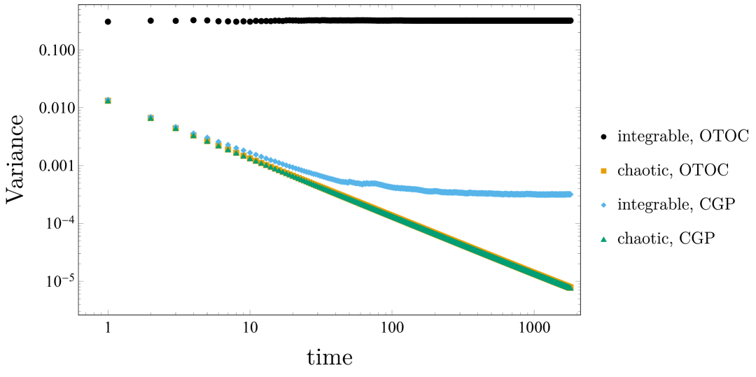
(a)

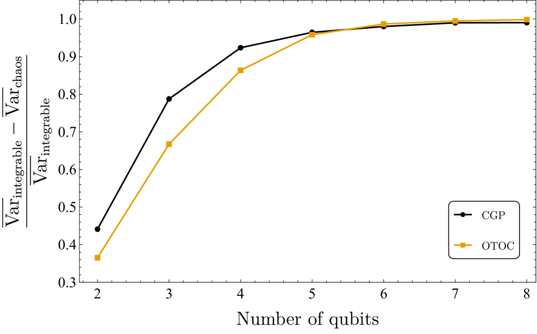
(b)

Figure 4: (a) Log-Log plot of the variance of CGP and OTOC for $n=9$ qubits. We study the dynamics of the Hamiltonian given by Eq. 43 with $g=1,h=0$ as the integrable limit and $g=-1.05,h=0.5$ as the chaotic one. We set, $V=\sigma_{1}^{z},W=\sigma^{z}_{9}$ for the OTOC and CGP in Eq. 20. (b) Fraction of the long-time average of the variance of chaotic and integrable OTOC, CGP, that is, $\frac{\overline{\mathrm{Var}}_{\mathrm{integrable}}-\overline{\mathrm{Var}}_{\mathrm{chaos}}}{\overline{\mathrm{Var}}_{\mathrm{integrable}}}$ for the Hamiltonian given by Eq. 43 with $g=1,h=0$ as the integrable limit and $g=-1.05,h=0.5$ as the chaotic one. We set, $V=\sigma_{1}^{z},W=\sigma^{z}_{9}$ for the OTOC and CGP in Eq. 20.

OTOCs capture the scrambling of quantum information. As localized information spreads through the nonlocal degrees of freedom of a system, it becomes inaccessible to local observables and their expectation values reveal an equilibration of the subsystem state. This apparent irreversible loss of information under unitary dynamics (which is reversible) has been termed scrambling. Signatures of scrambling can be observed in the long-time averages of both simple physical quantities like local expectation values and in “complex” quantities such as the OTOC and CGP. However, in finite systems, such long-time averages do not converge in the limit $t\rightarrow\infty$, instead they typically oscillate around some equilibrium value. This equilibrium value can be obtained from the infinite-time average, $\overline{A}\coloneqq\lim_{T\rightarrow\infty}\frac{1}{T}\int\limits_{0}^{T}A(t)dt$. In Ref. Styliaris et al. (2020), the infinite-time average of the averaged OTOC (with a bipartition in the system Hilbert space) was studied for both integrable and chaotic models and its equilibration value was used to successfully distinguish the two phases; see also related work studying the long-time limit of OTOCs for the integrability-to-chaos transition García-Mata et al. (2018); Fortes et al. (2019). Along the way, connections with entropy production, operator entanglement, and channel distinguishability were also discussed.

It was previously shown that in the long-time limit, the strength of recurrences can distinguish chaotic and integrable systems Campos Venuti (2015); Fishman et al. (1982). Let $n$ be the number of qubits (or more generally, the system size), then integrable systems typically have a quantum recurrence time that is a polynomial in $n$, while chaotic systems typically have recurrence times that are doubly exponential in $n$, that is, $O(e^{e^{n}})$. Therefore, when studying recurrences in the expectation values of observables for a finite (but large) time, one expects integrable systems to show larger recurrences than chaotic systems. Building on the work of Refs. Hosur et al. (2016); Cotler et al. (2017), we show that by considering the OTOC and the CGP as “complex observables” and quantifying their recurrences via their temporal variance, one can distinguish integrable and chaotic regimes. We also argue that for the purposes of distinguishing these two phases via the strength of their recurrences, the OTOC and CGP capture effectively the same behavior, vindicating our 3.

The physical system we use to study this temporal variance is the paradigmatic transverse-field Ising model with open boundary conditions,

$$H_{\mathrm{TFIM}}=-\left(\sum\limits_{j=1}^{L-1}\sigma^{z}_{j}\sigma^{z}_{j+1}+\sum\limits_{j=1}^{L}g\sigma^{x}_{j}+h\sigma^{z}_{j}\right).$$ (43)

The system has an integrable limit for $h=0$, where the Hamiltonian can be mapped onto free fermions; we set $g=1,h=0$ as the integrable point. The system is quantum chaotic for the parameter choices $g=-1.05,h=0.5$ which can be seen, for example, by studying the level spacing distribution. In Ref. Hosur et al. (2016), the OTOC averaged over local observables was used to distinguish the two phases and it was observed that in the chaotic limit, the system quickly asymptotes to just below the Haar-averaged value, while in the integrable regime, the systems displays large recurrences and does not show any features of scrambling. A similar behavior was observed for the mutual information between different subsystems. Here, we compare the dynamical behavior of the OTOC and the CGP for $V=\sigma^{z}_{1},W=\sigma_{L}^{z}$ for an $L$-site system. Notice that our numerical simulations use exact dynamics but are limited to timescales far below the expected recurrence time for the chaotic limit. However, we are able to observe and quantify recurrences for the integrable case in a way that is sufficient to distinguish the two phases.

For systems satisfying the ETH Ansatz Srednicki (1994); Deutsch (1991); Rigol et al. (2008), fluctuations around the long-time averages of expectation values of observables will be exponentially small in the system size D’Alessio et al. (2016); Borgonovi et al. (2016). While the CGP and OTOC are “complex” quantities, their behavior can be expected to resemble that of simpler observables, especially for finite systems and simple local operators such as Pauli matrices. Since quantum chaotic systems typically obey the ETH Ansatz (after removing trivial symmetries), the fluctuations in the OTOC and CGP around their long-time average may be expected to become exponentially small in the system size. Our numerical findings summarized in Fig. 4 vindicate this intuition: we consider the long-time average of the OTOC and the CGP in the integrable and chaotic regimes. In the chaotic regime the variance of the CGP and the OTOC are equal up to numerical error ($\approx 10^{-10}$ in dimensionless units), while in the integrable regime the variance seems to asymptote to different values for the CGP and the OTOC – which is simply a consequence of the different timescales of recurrences in these two quantities. A more meaningful comparison can be obtained by computing the relative fluctuations in the integrable and chaotic regimes, for which we compute the ratio

$$\frac{\overline{\mathrm{Var}}_{\mathrm{integrable}}-\overline{\mathrm{Var}}_{\mathrm{chaos}}}{\overline{\mathrm{Var}}_{\mathrm{integrable}}},$$

where $\overline{\mathrm{Var}}_{\mathrm{integrable}}$ is the long-time average of the temporal variance of the CGP/OTOC in the integrable regime, performed numerically. We find that for both the OTOC and CGP, this quantity becomes exponentially close to one as a function of the system size. Therefore, the fluctuations around the average in the chaotic regime are exponentially smaller than that in the integrable case, as expected, and both the OTOC and its subpart, the CGP can diagnose chaoticity in this way.

V Discussion

While the role of quantum entanglement in characterizing quantum chaos has been widely explored, it remained unclear what precise role quantum coherence plays, if any, in diagnosing quantum chaos. Our work affirmatively answers this question by establishing rigorous connections between measures of quantum coherence and signatures of quantum chaos. Coherence of Hamiltonian eigenstates is shown to be an “order parameter” for the integrable-to-chaotic transition and we numerically demonstrate this by studying quantum chaos in an XXZ spin-chain with defect and find excellent agreement with random matrix theory (RMT) in the bulk of the spectrum, as expected. Furthermore, using the mathematical formalism of majorization theory and fundamental results from the resource theory of coherence, we argue why every quantum coherence measure is a “delocalization” measure — a class of signatures of quantum chaos that quantify spread, in say, the position eigenbasis, energy eigenbasis, and others. Moreover, our 2 shows that for pure states in a bipartite system, the $2$-coherence minimized over product bases is equal to the linear entropy of the reduced state. That is, quantum coherence measures can be used to detect the entanglement in a quantum state, as has also been demonstrated previously Streltsov et al. (2015).

For dynamical signatures of chaos, our 3 establishes the coherence-generating power (CGP) as a subpart of the OTOC, a prominent measure of information scrambling in quantum systems. In particular, the (associated) squared-commutator’s growth signals the increasing incompatibility of the operators under time-evolution. Our theorem paves a way to make this intuition precise as the CGP quantifies incompatibility between the bases associated to the time-evolving operator in the OTOC and the fixed one. Moreover, we analytically show, in many different ways, how the OTOC, suitably averaged, connects with $2$-coherence of a state, the CGP of dynamics, and the geometric distance between the MASAs associated to the bases of the operators in the OTOC. Among a plethora of other reasons, the CGP is particularly well-suited to quantify this incompatibility since it also happens to be a formal measure in the resource theory of measurement incompatibility Styliaris and Zanardi (2019).

Furthermore, using RMT we provide an upper bound on the average CGP for GUE Hamiltonians in terms of the Spectral Form Factor, a well-established measure of quantum chaos. We also find an analytical expression for the Haar-averaged OTOC-CGP relation, which allows us to argue that under certain assumptions, the OTOC is approximated exponentially-well (in the system size) by the CGP.

The short-time behavior of the OTOC has received considerable attention in recent years and so we analyze the short-time growth of the CGP (a subpart of the OTOC) which, to leading order, is characterized by the variance of the Hamiltonian with respect to a basis; for the OTOC this basis is inherited from the choice of the OTOC operators. We remark that this variance of the Hamiltonian (for pure states) is related to quantum speed limits and the resource theory of asymmetry Marvian et al. (2016). And finally, we numerically study the long-time behavior of the OTOC and CGP in a transverse-field Ising model and find that their temporal variances quantify chaos in effectively the same way.

In closing, our results establish quantum coherence as a signature of quantum chaos, both at the level of states and dynamics. As a future work, it would be interesting to see how well suited measures of quantum coherence are to the study few-body chaos, in particular, using paradigmatic systems like the quantum kicked top Wang et al. (2004). Few-body systems provide a powerful experimental testbed for studying signatures of thermalization and scrambling, which are intimately linked with quantum coherence measures. Quantitatively establishing these connections will also be a promising future direction.

VI Acknowledgments

N.A. would like to thank Todd Brun, Bibek Pokharel, and Evangelos Vlachos for many insightful discussions about quantum chaos. Research was funded by the Deutsche Forschungsgemeinschaft (DFG, German Research Foundation) under Germany’s Excellence Strategy – EXC-2111 – 390814868. This research was supported in part by Perimeter Institute for Theoretical Physics. Research at Perimeter Institute is supported in part by the Government of Canada through the Department of Innovation, Science and Economic Development Canada and by the Province of Ontario through the Ministry of Colleges and Universities. P.Z. acknowledges partial support from the NSF award PHY-1819189. This research was (partially) sponsored by the Army Research Office and was accomplished under Grant Number W911NF-20-1-0075. The views and conclusions contained in this document are those of the authors and should not be interpreted as representing the official policies, either expressed or implied, of the Army Research Office or the U.S. Government. The U.S. Government is authorized to reproduce and distribute reprints for Government purposes notwithstanding any copyright notation herein.

Appendices

Appendix A1 Level spacing distribution

(a)

(b)

(c)

(d)

Figure 5: The transition in level-spacing distribution from Poisson to the (universal) Wigner-Dyson distribution for the Hamiltonian described in Eq. 13 as we move the defectsite to the middle of the chain. Figures (a), (b), (c), and (d) correspond to the defect at sites $\delta=1,\delta=3,\delta=5,$ and $\delta=7$, respectively. Results are reported for $L=15$ with $5$ spins up and $\omega=0,\epsilon_{\delta}=0.5,J_{xy}=1,J_{z}=0.5$. Similar results were obtained for $L=15$ and $\delta=1,7$ in Ref. Gubin and F. Santos (2012) (but not for intermediate positions of the defect site).

Appendix A2 Coherence quantifiers for integrable and chaotic eigenstates

(a)

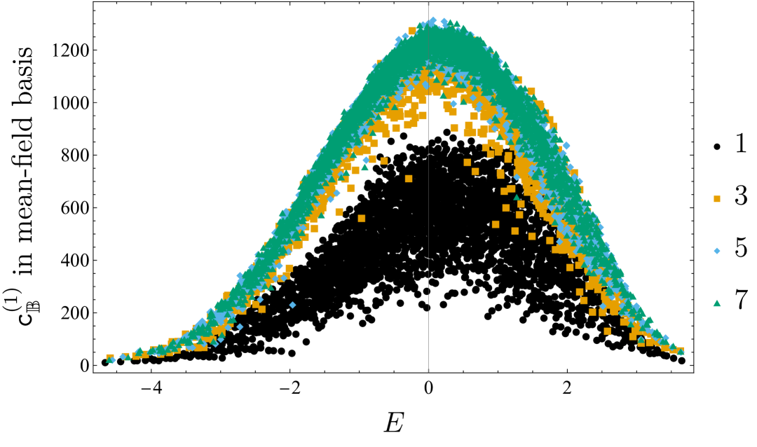
(b)

Figure 7: $1$-coherence for eigenstates of the Hamiltonian defined in Eq. 13 as a function of their energy. Results are reported for $L=15$ with $5$ spins up and $\omega=0,\epsilon_{\delta}=0.5,J_{xy}=1,J_{z}=0.5$. The plot markers $1,3,5,7$ correspond to the various choices of the defect site, with $\delta=1,7$ corresponding to the integrable and chaotic limits, respectively. Figures (a) and (b) correspond to the two different bases, the site-basis and the mean-field basis, respectively.

Appendix A3 Proofs

Here we restate the Propositions, Theorems, as well as other mathematical claims appearing in the main text, and give their proofs.

Proof of 2

See 2

Proof.

We start by collecting a few simple results. First, recall that the $2$-coherence is

$$\mathtt{c}^{(\mathrm{2})}_{\mathbb{B}}(\rho) =\left\|\rho-\mathcal{D}_{\mathbb{B}}(\rho)\right\|_{2}^{2}=\left\langle\rho-\mathcal{D}_{\mathbb{B}}(\rho),\rho-\mathcal{D}_{\mathbb{B}}(\rho)\right\rangle=\left\langle\rho,\rho\right\rangle-\left\langle\rho,\mathcal{D}_{\mathbb{B}}(\rho)\right\rangle-\left\langle\mathcal{D}_{\mathbb{B}}(\rho),\rho\right\rangle+\left\langle\mathcal{D}_{\mathbb{B}}(\rho),\mathcal{D}_{\mathbb{B}}(\rho)\right\rangle$$ (A1)

$$=\left\langle\rho,\rho\right\rangle-\left\langle\rho,\mathcal{D}_{\mathbb{B}}(\rho)\right\rangle,$$ (A2)

where in the second line, we have used $\left\langle\rho,\mathcal{D}_{\mathbb{B}}(\rho)\right\rangle=\left\langle\mathcal{D}_{\mathbb{B}}(\rho),\rho\right\rangle$ since $\mathcal{D}_{\mathbb{B}}$ is a self-adjoint superoperator and $\left\langle\mathcal{D}_{\mathbb{B}}(\rho),\mathcal{D}_{\mathbb{B}}(\rho)\right\rangle=\left\langle\rho,\mathcal{D}_{\mathbb{B}}(\rho)\right\rangle$ since $\mathcal{D}_{\mathbb{B}}$ is a projection superoperator, that is, $(\mathcal{D}_{\mathbb{B}})^{2}=\mathcal{D}_{\mathbb{B}}$.

For pure states, we have, $\left\langle\rho,\rho\right\rangle=1$ and therefore, the $2$-coherence for pure states is equal to $\mathtt{c}^{(\mathrm{2})}_{\mathbb{B}}(\rho)=1-\left\langle\rho,\mathcal{D}_{\mathbb{B}}(\rho)\right\rangle$.

Second, a pure bipartite state, $|\Psi\rangle_{AB}\in\mathcal{H}\cong\mathcal{H}_{A}\otimes\mathcal{H}_{B}$ can be written in the Schmidt form (that is, using Schmidt decomposition theorem) Nielsen and Chuang (2010),

$$|\Psi\rangle_{AB}=\sum\limits_{j=1}^{\mathrm{min}\left\{d_{A},d_{B}\right\}}\lambda_{j}|j\rangle_{A}\otimes|\widetilde{j}\rangle_{B},$$ (A3)

where $\{|j\rangle_{A}\},\{|\widetilde{j}\rangle_{B}\}$ is an orthonormal basis for subsystems A, B, respectively, and $\{\lambda_{j}\}$ are non-negative coefficients satisfying $\sum\limits_{j}\lambda_{j}^{2}=1$. The coefficients $\lambda_{j}^{2}$ are the eigenvalues of the reduced density matrix $\rho_{A}$; recall also that $\rho_{A}$ and $\rho_{B}$ are isospectral. Then, re-expressing the state in this form, we have (dropping the subscripts for the subsytems $A,B$),

$$|\Psi\rangle\langle\Psi|=\sum\limits_{j,k}\lambda_{j}\lambda_{k}|j\rangle\langle k|\otimes|\widetilde{j}\rangle\langle\widetilde{k}|.$$ (A4)

And third, the dephasing superoperator factorizes, that is,

$$\mathcal{D}_{\mathbb{B}_{a}\otimes\mathbb{B}_{b}}=\mathcal{D}_{\mathbb{B}_{a}}\otimes\mathcal{D}_{\mathbb{B}_{b}}.$$ (A5)

To see this, let $\mathbb{B}_{a}=\{\Pi_{j}^{(a)}\}_{j=1}^{d}$ and $\mathbb{B}_{b}=\{\Pi_{k}^{(b)}\}_{k=1}^{d}$, then, the action of $\mathcal{D}_{\mathbb{B}_{a}\otimes\mathbb{B}_{b}}$ is

$$\mathcal{D}_{\mathbb{B}_{a}\otimes\mathbb{B}_{b}}(X)=\sum\limits_{j,k=1}^{d}\left(\Pi_{j}^{(a)}\otimes\Pi_{k}^{(b)}\right)X\left(\Pi_{j}^{(a)}\otimes\Pi_{k}^{(b)}\right)$$ (A6)

and the action of $\mathcal{D}_{\mathbb{B}_{a}}\otimes\mathcal{D}_{\mathbb{B}_{b}}$ is,

$$\mathcal{D}_{\mathbb{B}_{a}}\otimes\mathcal{D}_{\mathbb{B}_{b}}(X) =\mathcal{D}_{\mathbb{B}_{a}}\left(\sum\limits_{k=1}^{d}\left(\mathbb{I}\otimes\Pi_{k}^{(b)}\right)X\left(\mathbb{I}\otimes\Pi_{k}^{(b)}\right)\right)$$ (A7)

$$=\sum\limits_{j,k=1}^{d}\left(\Pi_{j}^{(a)}\otimes\mathbb{I}\right)\left(\mathbb{I}\otimes\Pi_{k}^{(b)}\right)X\left(\mathbb{I}\otimes\Pi_{k}^{(b)}\right)\left(\Pi_{j}^{(a)}\otimes\mathbb{I}\right)$$ (A8)

$$=\sum\limits_{j,k=1}^{d}\left(\Pi_{j}^{(a)}\otimes\Pi_{k}^{(b)}\right)X\left(\Pi_{j}^{(a)}\otimes\Pi_{k}^{(b)}\right)=\mathcal{D}_{\mathbb{B}_{a}\otimes\mathbb{B}_{b}}(X).$$ (A9)

We are now ready to prove the main result.

$$\min_{\mathbb{B}_{a},\mathbb{B}_{b}}\mathtt{c}^{(\text{2})}_{\mathbb{B}_{a}\otimes\mathbb{B}_{b}}(|\Psi\rangle\langle\Psi|)=\min_{\mathbb{B}_{a},\mathbb{B}_{b}}\left\{1-\left\langle|\Psi\rangle\langle\Psi|,\mathcal{D}_{\mathbb{B}_{a}\otimes\mathbb{B}_{b}}\left(|\Psi\rangle\langle\Psi|\right)\right\rangle\right\}=1-\max_{\mathbb{B}_{a},\mathbb{B}_{b}}\left\{\left\langle|\Psi\rangle\langle\Psi|,\mathcal{D}_{\mathbb{B}_{a}\otimes\mathbb{B}_{b}}\left(|\Psi\rangle\langle\Psi|\right)\right\rangle\right\}.$$ (A10)

Let us consider the term inside the maximization, $\left\langle|\Psi\rangle\langle\Psi|,\mathcal{D}_{\mathbb{B}_{a}\otimes\mathbb{B}_{b}}\left(|\Psi\rangle\langle\Psi|\right)\right\rangle$. We use the Schmidt form of $|\Psi\rangle$ and substitute $\mathcal{D}_{\mathbb{B}_{a}\otimes\mathbb{B}_{b}}$ by $\mathcal{D}_{\mathbb{B}_{a}}\otimes\mathcal{D}_{\mathbb{B}_{b}}$ to get

$$\left\langle|\Psi\rangle\langle\Psi|,\mathcal{D}_{\mathbb{B}_{a}\otimes\mathbb{B}_{b}}\left(|\Psi\rangle\langle\Psi|\right)\right\rangle =\sum\limits_{j,k,l,m}^{d}\lambda_{j}\lambda_{k}\lambda_{l}\lambda_{m}\operatorname{Tr}\left(|l\rangle\langle m|\otimes|\widetilde{l}\rangle\langle\widetilde{m}|\mathcal{D}_{\mathbb{B}_{a}}\left(|j\rangle\langle k|\right)\otimes\mathcal{D}_{\mathbb{B}_{b}}\left(|\widetilde{j}\rangle\langle\widetilde{k}|\right)\right)$$ (A11)

$$=\sum\limits_{j,k,l,m}^{d}\lambda_{j}\lambda_{k}\lambda_{l}\lambda_{m}\operatorname{Tr}\left(|l\rangle\langle m|\mathcal{D}_{\mathbb{B}_{a}}\left(|j\rangle\langle k|\right)\right)\operatorname{Tr}\left(|\widetilde{l}\rangle\langle\widetilde{m}|\mathcal{D}_{\mathbb{B}_{b}}\left(|\widetilde{j}\rangle\langle\widetilde{k}|\right)\right).$$ (A12)

It is easy to see that to maximize these inner products, we need to choose the dephasing basis to be the same as the local basis $\{|j\rangle\},\{|\widetilde{j}\rangle\}$, respectively. To see this, let $\mathbb{B}_{a}=\{|\phi_{j}\rangle\langle\phi_{j}|\}$, then, the term $\operatorname{Tr}\left(|l\rangle\langle m|\mathcal{D}_{\mathbb{B}_{a}}\left(|j\rangle\langle k|\right)\right)$ becomes,

$$\sum\limits_{j=1}^{d}\langle\phi_{j}|l\rangle\langle m|\phi_{j}\rangle\langle\phi_{j}|j\rangle\langle k|\phi_{j}\rangle,$$ (A13)

an upper bound on which can be obtained using Cauchy-Schwarz inequality repeatedly to see that it is maximized when $|\phi_{j}\rangle=|j\rangle\leavevmode\nobreak\ \leavevmode\nobreak\ \forall j$. That is, the local basis in the Schmidt decomposition of the state and the dephasing basis are the same. Therefore, $\mathcal{D}_{\mathbb{B}_{a}}\left(|j\rangle\langle k|\right)=|j\rangle\langle k|\delta_{j,k}$ and $\mathcal{D}_{\mathbb{B}_{b}}\left(|\widetilde{j}\rangle\langle\widetilde{k}|\right)=|\widetilde{j}\rangle\langle\widetilde{k}|\delta_{j,k}$. Plugging it back, we have,

$$\max_{\mathbb{B}_{a},\mathbb{B}_{b}}\left\{\left\langle|\Psi\rangle\langle\Psi|,\mathcal{D}_{\mathbb{B}_{a}\otimes\mathbb{B}_{b}}\left(|\Psi\rangle\langle\Psi|\right)\right\rangle\right\}=\sum\limits_{j,k,l,m}^{d}\lambda_{j}\lambda_{k}\lambda_{l}\lambda_{m}\delta_{jk}\delta_{m,j}\delta_{l,j}=\sum\limits_{j=1}^{d}\lambda_{j}^{4}=\left\|\rho_{a}\right\|_{2}^{2}.$$ (A14)

Therefore, putting everything together, we have,

$$\min_{\mathbb{B}_{a},\mathbb{B}_{b}}\mathtt{c}^{(\text{2})}_{\mathbb{B}_{a}\otimes\mathbb{B}_{b}}(|\Psi\rangle\langle\Psi|)=1-\left\|\rho_{a}\right\|_{2}^{2}=:S_{\text{lin}}(\rho_{a}).$$ (A15)

∎

Proof of 3

See 3

Proof.

Consider the infinite-temperature OTOC, $C^{(\beta=0)}_{V,W}(t)=\frac{1}{d}\operatorname{Tr}\left(\left[V,W(t)\right]^{\dagger}\left[V,W(t)\right]\right)$. Then, plugging in the spectral decomposition of $V,W$, that is, $V=\sum\limits_{j}v_{j}\Pi_{j},W(t)=\sum\limits_{j}w_{j}\widetilde{\Pi}_{j}(t)$, we have

$$C_{V,W}(t)=\frac{1}{d}\sum\limits_{j,k,l,m}v_{j}^{*}w_{k}^{*}v_{l}w_{m}\operatorname{Tr}\left(\left[\Pi_{j},\widetilde{\Pi}_{k}(t)\right]^{\dagger}\left[\Pi_{l},\widetilde{\Pi}_{m}(t)\right]\right).$$

Then, extracting the $j=l$ and $k=m$ terms, we have,

$$C_{V,W}(t)=\frac{1}{d}\sum\limits_{j,k}\left|v_{j}\right|^{2}\left|w_{k}\right|^{2}\operatorname{Tr}\left(\left[\Pi_{j},\widetilde{\Pi}_{k}(t)\right]^{\dagger}\left[\Pi_{j},\widetilde{\Pi}_{k}(t)\right]\right)+\frac{1}{d}\sum\limits_{j\neq l,k\neq m}v_{j}^{*}w_{k}^{*}v_{l}w_{m}\operatorname{Tr}\left(\left[\Pi_{j},\widetilde{\Pi}_{k}(t)\right]^{\dagger}\left[\Pi_{l},\widetilde{\Pi}_{m}(t)\right]\right).$$ (A16)

Since, $V,W$ are unitary, we have, $\left|v_{j}\right|^{2}=1=\left|w_{j}\right|^{2}\leavevmode\nobreak\ \leavevmode\nobreak\ \forall j\in\{1,2,\cdots,d\}$. Therefore,

$$C_{V,W}(t)=\frac{1}{d}\sum\limits_{j,k}\operatorname{Tr}\left(\left[\Pi_{j},\widetilde{\Pi}_{k}(t)\right]^{\dagger}\left[\Pi_{j},\widetilde{\Pi}_{k}(t)\right]\right)+\frac{1}{d}\sum\limits_{j\neq l,k\neq m}v_{j}^{*}w_{k}^{*}v_{l}w_{m}\operatorname{Tr}\left(\left[\Pi_{j},\widetilde{\Pi}_{k}(t)\right]^{\dagger}\left[\Pi_{l},\widetilde{\Pi}_{m}(t)\right]\right).$$ (A17)

Then, recalling Eq. 19, we have,

$$C_{V,W}(t)=2\mathfrak{C}_{\mathbb{B}_{V}}\left(\mathcal{U}_{t}\circ\mathcal{V}_{\mathbb{B}_{V}\rightarrow\mathbb{B}_{W}}\right)+\frac{1}{d}\sum\limits_{j\neq l,k\neq m}v_{j}^{*}w_{k}^{*}v_{l}w_{m}\operatorname{Tr}\left(\left[\Pi_{j},\widetilde{\Pi}_{k}(t)\right]^{\dagger}\left[\Pi_{l},\widetilde{\Pi}_{m}(t)\right]\right),$$ (A18)

where $\mathcal{V}_{\mathbb{B}_{V}\rightarrow\mathbb{B}_{W}}$ is the intertwiner connecting the bases $\mathbb{B}_{V}$ to $\mathbb{B}_{W}$ as $\mathcal{V}_{\mathbb{B}_{V}\rightarrow\mathbb{B}_{W}}\left(\Pi_{j}\right)=\widetilde{\Pi}_{j}\leavevmode\nobreak\ \leavevmode\nobreak\ \forall j\in\{1,2,\cdots,d\}$.

Next, we would like to simplify the second term of the summation. For this, note that

$$\operatorname{Tr}\left(\left[\Pi_{j},\widetilde{\Pi}_{k}(t)\right]^{\dagger}\left[\Pi_{l},\widetilde{\Pi}_{m}(t)\right]\right)=\operatorname{Tr}\left(\left\{\widetilde{\Pi}_{k}\Pi_{j}-\Pi_{j}\widetilde{\Pi}_{k}\right\}\left\{\Pi_{l}\widetilde{\Pi}_{m}-\widetilde{\Pi}_{m}\Pi_{l}\right\}\right)$$ (A19)

$$=\operatorname{Tr}\left(\widetilde{\Pi}_{k}\Pi_{j}\Pi_{l}\widetilde{\Pi}_{m}\right)-\operatorname{Tr}\left(\widetilde{\Pi}_{k}\Pi_{j}\widetilde{\Pi}_{m}\Pi_{l}\right)-\operatorname{Tr}\left(\Pi_{j}\widetilde{\Pi}_{k}\Pi_{l}\widetilde{\Pi}_{m}\right)+\operatorname{Tr}\left(\Pi_{j}\widetilde{\Pi}_{k}\widetilde{\Pi}_{m}\Pi_{l}\right)$$ (A20)

$$=\delta_{km}\delta_{jl}\operatorname{Tr}\left(\Pi_{j}\widetilde{\Pi}_{k}\right)-\operatorname{Tr}\left(\widetilde{\Pi}_{k}\Pi_{j}\widetilde{\Pi}_{m}\Pi_{l}\right)-\operatorname{Tr}\left(\Pi_{j}\widetilde{\Pi}_{k}\Pi_{l}\widetilde{\Pi}_{m}\right)+\delta_{jl}\delta_{km}\operatorname{Tr}\left(\Pi_{j}\widetilde{\Pi}_{k}\right)$$ (A21)

$$=2\delta_{km}\delta_{jl}\operatorname{Tr}\left(\Pi_{j}\widetilde{\Pi}_{k}\right)-2\mathfrak{Re}\left\{\operatorname{Tr}\left(\widetilde{\Pi}_{k}\Pi_{j}\widetilde{\Pi}_{m}\Pi_{l}\right)\right\}.$$ (A22)

The summation indices for the second term are $j\neq l$ OR $k\neq m$, which has three possibilities: $j\neq l\text{ and }k\neq m$, $j\neq l\text{ but }k=m$, and finally, $j=l\text{ but }k\neq m$. In each case, the product of delta functions, $\delta_{km}\delta_{jl}$ vanishes and we are left with the second term only. Therefore,

$$C_{V,W}(t)=2\mathfrak{C}_{\mathbb{B}_{V}}\left(\mathcal{U}_{t}\circ\mathcal{V}_{\mathbb{B}_{V}\rightarrow\mathbb{B}_{W}}\right)-\frac{2}{d}\mathfrak{Re}\left\{\sum\limits_{j\neq l,k\neq m}v_{j}^{*}w_{k}^{*}v_{l}w_{m}\operatorname{Tr}\left(\widetilde{\Pi}_{k}(t)\Pi_{j}\widetilde{\Pi}_{m}(t)\Pi_{l}\right)\right\},$$ (A23)

where we emphasize that the indices of the summation have the three possibilities listed above.

The relation between $F_{V,W}(t)$ and $\mathfrak{C}_{\mathbb{B}_{V}}$ is obtained simply by using $C_{V,W}(t)=2\left(1-\mathfrak{Re}\left\{F_{V,W}(t)\right\}\right)$. This completes the proof. ∎

Proof of Equation 26, Equation 28, and Equation 30

Let’s start with Equation 30. We have two unitaries $V,W$ and two bases $\mathbb{B},\widetilde{\mathbb{B}}$. Then, the following Haar-averaged squared commutator is proportional to the (squared) distance in the Grassmannian between the MASAs associated to the bases $\mathbb{B},\mathbb{\widetilde{B}}$. That is,

$$\left\langle\left\|\left[\mathcal{D}_{\mathbb{B}}(V),\mathcal{D}_{\widetilde{\mathbb{B}}}(W)\right]\right\|_{2}^{2}\right\rangle_{V,W\in\mathrm{Haar}}=\frac{1}{d^{2}}D^{2}(\mathcal{A}_{\mathbb{B}},\mathcal{A}_{\widetilde{\mathbb{B}}})$$ (A24)

We start by expanding $\left\|\left[\mathcal{D}_{\mathbb{B}}(V),\mathcal{D}_{\widetilde{\mathbb{B}}}(W)\right]\right\|_{2}^{2}$ with $v_{\alpha}\coloneqq\operatorname{Tr}\left(\Pi_{\alpha}V\right),w_{\beta}\coloneqq\operatorname{Tr}\left(\widetilde{\Pi}_{\beta}W\right)$. Then,

$$\left\|\left[\mathcal{D}_{\mathbb{B}}(V),\mathcal{D}_{\widetilde{\mathbb{B}}}(W)\right]\right\|_{2}^{2}=\left\|\sum\limits_{\alpha,\beta}^{d}v_{\alpha}w_{\beta}\left[\Pi_{\alpha},\widetilde{\Pi}_{\beta}\right]\right\|_{2}^{2}=\sum\limits_{\alpha,\beta,\gamma,\eta}^{d}v_{\alpha}^{*}w_{\beta}^{*}v_{\gamma}w_{\eta}\operatorname{Tr}\left(\left[\Pi_{\alpha},\widetilde{\Pi}_{\beta}\right]^{\dagger}\left[\Pi_{\gamma},\widetilde{\Pi}_{\eta}\right]\right).$$ (A25)

Now, $v_{\alpha}^{*}v_{\gamma}=\operatorname{Tr}\left(\Pi_{\alpha}V^{\dagger}\right)\operatorname{Tr}\left(\Pi_{\gamma}V\right)=\operatorname{Tr}\left(\left(\Pi_{\alpha}\otimes\Pi_{\gamma}\right)\left(V^{\dagger}\otimes V\right)\right)$ and using the lemma,

$$\int_{\mathrm{Haar}}dAA^{\dagger}\otimes A=\frac{S}{d},\text{ where S is the SWAP operator,}$$ (A26)

we have

$$\left\langle v_{\alpha}^{*}v_{\gamma}\right\rangle_{V\in\mathrm{Haar}}=\int_{\mathrm{Haar}}dV\operatorname{Tr}\left(\left(\Pi_{\alpha}\otimes\Pi_{\gamma}\right)\left(V^{\dagger}\otimes V\right)\right)=\frac{1}{d}\operatorname{Tr}\left(\left(\Pi_{\alpha}\otimes\Pi_{\gamma}\right)S\right)=\frac{1}{d}\operatorname{Tr}\left(\Pi_{\alpha}\Pi_{\gamma}\right)=\frac{1}{d}\delta_{\alpha,\gamma}.$$ (A27)

Similarly, for $\left\langle w_{\beta}^{*}w_{\eta}\right\rangle_{W\in\mathrm{Haar}}=\frac{1}{d}\delta_{\beta,\eta}$. Putting everything together, we have,

$$\left\langle\left\|\left[\mathcal{D}_{\mathbb{B}}(V),\mathcal{D}_{\widetilde{\mathbb{B}}}(W)\right]\right\|_{2}^{2}\right\rangle_{V,W\in\mathrm{Haar}}=\frac{1}{d^{2}}\sum\limits_{\alpha,\beta,\gamma,\eta}^{d}\delta_{\alpha,\gamma}\delta_{\beta,\eta}\operatorname{Tr}\left(\left[\Pi_{\alpha},\widetilde{\Pi}_{\beta}\right]^{\dagger}\left[\Pi_{\gamma},\widetilde{\Pi}_{\eta}\right]\right)=\frac{1}{d^{2}}\sum\limits_{\alpha,\beta}^{d}\left\|\left[\Pi_{\alpha},\widetilde{\Pi}_{\beta}\right]\right\|_{2}^{2}=\frac{1}{d^{2}}D^{2}(\mathcal{A}_{\mathbb{B}},\mathcal{A}_{\widetilde{\mathbb{B}}}).$$ (A28)

To prove Equation 28, $\left\langle\left\|\left[\mathcal{D}_{\mathbb{B}}(V),\rho\right]\right\|_{2}^{2}\right\rangle_{V\in\mathrm{Haar}}=\frac{2}{d}\mathrm{c}_{\mathbb{B}}^{(2)}(\rho)$, we follow a similar sequence of arguments as above. We prove a slightly general version of the result here, where $V$ is a unitary and $X$ an arbitrary operator (and not necessarily a quantum state)

$$\left\|\left[\mathcal{D}_{\mathbb{B}}(V),X\right]\right\|_{2}^{2}=\sum\limits_{\alpha,\beta}^{d}v_{\alpha}^{*}v_{\beta}\operatorname{Tr}\left(\left[\Pi_{\alpha},X\right]^{\dagger}\left[\Pi_{\beta},X\right]\right).$$ (A29)

As above, $\left\langle v_{\alpha}^{*}v_{\beta}\right\rangle_{V\in\mathrm{Haar}}=\frac{1}{d}\delta_{\alpha,\beta}$. Therefore,

$$\left\langle\left\|\left[\mathcal{D}_{\mathbb{B}}(V),X\right]\right\|_{2}^{2}\right\rangle_{V\in\mathrm{Haar}}=\frac{1}{d}\sum\limits_{\alpha}^{d}\left\|\left[\Pi_{\alpha},X\right]\right\|_{2}^{2}=\frac{2}{d}\mathrm{c}_{\mathbb{B}}^{(2)}(X).$$ (A30)

And finally, to prove Equation 26, $\left\langle\left\|\left[V,W(t)\right]\right\|_{2}^{2}\right\rangle_{\theta}=2d\mathfrak{C}_{\mathbb{B}_{V}}\left(\mathcal{U}_{t}\circ\mathcal{V}_{\mathbb{B}_{V}\rightarrow\mathbb{B}_{W}}\right)$, we proceed as above and note that the key step is $\left\langle v_{\alpha}^{*}v_{\gamma}\right\rangle_{\theta}=\left\langle e^{i(\theta_{\gamma}-\theta_{\alpha})}\right\rangle_{\theta}=\frac{1}{2\pi}\int\limits_{0}^{2\pi}e^{i\left(\theta_{\gamma}-\theta_{\alpha}\right)}d\theta=\delta_{\alpha,\gamma}$. And similarly for $\left\langle w_{\beta}^{*}w_{\eta}\right\rangle_{\theta}=\delta_{\beta,\eta}$. Putting everything together, we then have the desired result.

Proof of 4

See 4

Proof.

Let $\hat{S}$ be the SWAP operator defined in Eq. A40. Then,

$$\mathfrak{C}_{\mathbb{B}}\left(e^{-iHt}\right) \leq 1-\frac{1}{d}\sum\limits_{j}\left[\operatorname{Tr}{\left(P_{j}UP_{j}U^{\dagger}\right)}\right]^{2}$$ (A31)

$$=1-\frac{1}{d}\sum\limits_{j}\operatorname{Tr}\left({P_{j}}^{\otimes 2}U^{\otimes 2}{P_{j}}^{\otimes 2}{U^{\dagger}}^{\otimes 2}\right)$$ (A32)

$$=1-\frac{1}{d}\sum\limits_{j}\operatorname{Tr}\left(\hat{S}P_{j}^{\otimes 4}\left(U^{\otimes 2}\otimes{U^{\dagger}}^{\otimes 2}\right)\right)$$ (A33)

$$=1-\frac{1}{d}\sum\limits_{j}\sum\limits_{k,l,m,n}\operatorname{Tr}\left(P_{j}^{\otimes 4}V^{\otimes 4}\left(P_{k}\otimes P_{l}\otimes P_{m}\otimes P_{n}\right)\right)\times e^{-i\left(E_{k}+E_{l}-E_{m}-E_{n}\right)t},$$ (A34)

where in the first inequality, we have dropped the off-diagonal terms in the CGP, that is, using $\mathfrak{C}_{\mathbb{B}}\left(U\right)=1-1/d\sum_{j,k}\left[\operatorname{Tr}\left(\Pi_{j}U\Pi_{k}U^{\dagger}\right)\right]^{2}$ (see Eq. 18) and only keeping the terms with $j=k$. In the second line, we have simply re-expressed the trace by using $\left[\operatorname{Tr}(A)\right]^{2}=\operatorname{Tr}(A\otimes A)$. And, in the last line we have plugged in $U=\sum\limits_{k}e^{-iE_{k}t}VP_{k}V^{\dagger}$, where $\mathcal{V}(\cdot)=V(\cdot)V^{\dagger}$ is the unitary intertwiner connecting the Hamiltonian eigenbasis with the basis $\mathbb{B}$.

In the following we will make a simple change of notation for both convenience and consistency with other works: $E_{j}\mapsto\lambda_{j}$. Now, recall that for GUE, we have, $P(H)\propto\exp\left(-\frac{d}{2}\operatorname{Tr}\left(H^{2}\right)\right)$, therefore,

$$\int dHP(H)=\int d\lambda P(\lambda)\times\int dV,$$ (A35)

where the average decomposes into the eigenvalues and the eigenvectors. Recall that $V$ is Haar-distributed. Then,

$$P(\lambda)=c\left|\Delta(\lambda)\right|^{2}e^{-\frac{d}{2}\sum\limits_{j}\lambda_{j}^{2}},\text{ where }\Delta(\lambda)\equiv\prod_{1\leq j<k\leq d}\left(\lambda_{j}-\lambda_{k}\right)\text{ is the Vandermonde matrix.}$$ (A36)

Then,

$$\left\langle\mathfrak{C}_{\mathbb{B}}(e^{-iHt})\right\rangle_{\mathrm{GUE}} \leq 1-\frac{1}{d}\sum\limits_{j}\sum\limits_{k,l,m,n}\left(\int d\lambda P(\lambda)e^{-i\left(\lambda_{k}+\lambda_{l}-\lambda_{m}-\lambda_{l}\right)t}\times\int dV\operatorname{Tr}\left(P_{j}^{\otimes 4}\mathcal{V}^{\otimes 4}\left(P_{k}\otimes P_{l}\otimes P_{m}\otimes P_{n}\right)\right)\right).$$ (A37)

Notice that if $\lambda_{j}=\lambda_{k}$ for any $j,k$ then $\Delta(\lambda)=0$. Therefore, in the summation $\sum\limits_{k,l,m,n}$, we only need to consider $\lambda_{k}\neq\lambda_{l}\neq\lambda_{m}\neq\lambda_{n}$. Then, one can show that, $\int dV\operatorname{Tr}\left(P_{j}^{\otimes 4}\mathcal{V}^{\otimes 4}\left(P_{k}\otimes P_{l}\otimes P_{m}\otimes P_{n}\right)\right)=\frac{1}{d(d+1)(d+2)(d+3)}$; see Ref. Puchała and Miszczak (2011) for integrals of this form. Therefore,

$$\left\langle\mathfrak{C}_{\mathbb{B}}\left(e^{-iHt}\right)\right\rangle_{\mathrm{GUE}}\leq 1-\frac{1}{d(d+1)(d+2)(d+3)}\underbrace{\sum\limits_{k,l,m,n}\int e^{-i\left(\lambda_{k}+\lambda_{l}-\lambda_{m}-\lambda_{n}\right)t}P(\lambda)d\lambda}_{\mathcal{R}_{4}}.$$ (A38)

To see that the bound is tight for short times, notice that in order to establish the connection to the spectral form factor, the first step in the proof is the inequality, $\mathfrak{C}_{\mathbb{B}}\left(e^{-iHt}\right)\leq 1-\frac{1}{d}\sum_{j}\left[\operatorname{Tr}\left(P_{j}UP_{j}U^{\dagger}\right)\right]^{2}$ which is obtained by ignoring the off-diagonal terms in the CGP, $\mathfrak{C}_{\mathbb{B}}(U)=1-1/d\sum_{j,k}\left[\operatorname{Tr}\left(\Pi_{j}U\Pi_{k}U^{\dagger}\right)\right]^{2}$ (we drop the $j\neq k$ terms). Now, for short times, let $t=O(\epsilon)$, then, the contribution from the off-diagonal terms scales as $O(\epsilon^{4})\ll 1$, making the bound tight. ∎

Proof of 5

See 5

Proof.

First, note that using 3, we can Haar-average the CGP and the “off-diagonal” terms independently. Following Refs. Zanardi et al. (2017a); Styliaris et al. (2019), we have that

$$\left\langle\mathfrak{C}_{\mathbb{B}}\left(\mathcal{U}\right)\right\rangle_{\mathrm{Haar}}=\frac{\left(d-1\right)}{\left(d+1\right)}.$$ (A39)

Now, for the “off-diagonal” term, let us look at terms of the form $\operatorname{Tr}\left(\widetilde{\Pi}_{k}(t)\Pi_{j}\widetilde{\Pi}_{m}(t)\Pi_{l}\right)$. Let $\mathcal{H}=\mathcal{H}_{A}\otimes\mathcal{H}_{A^{\prime}}$, where $\mathcal{H}_{A}\cong\mathcal{H}_{A^{\prime}}$, that is, we take two copies of the Hilbert space. The SWAP operator acting on this doubled space is defined as,

$$\hat{S}=\sum_{i,j}|i\rangle_{A}\langle j|\otimes|j\rangle_{A^{\prime}}\langle i|.$$ (A40)

It is easy to show that $\operatorname{Tr}\left(XY\right)=\operatorname{Tr}\left(\hat{S}X\otimes Y\right)$, which we use in the following (and variants thereof). Then,

$$\operatorname{Tr}\left(\widetilde{\Pi}_{k}(t)\Pi_{j}\widetilde{\Pi}_{m}(t)\Pi_{l}\right)=\operatorname{Tr}\left(\Pi_{l}\widetilde{\Pi}_{k}(t)\otimes\Pi_{j}\widetilde{\Pi}_{m}(t)\hat{S}\right)$$ (A41)

$$=\operatorname{Tr}\left(\left(\Pi_{l}\otimes\Pi_{j}\right)\left(\widetilde{\Pi}_{k}(t)\otimes\widetilde{\Pi}_{m}(t)\right)\hat{S}\right)=\operatorname{Tr}\left(\left(\Pi_{l}\otimes\Pi_{j}\right)\mathcal{U}_{t}^{\otimes 2}\left(\widetilde{\Pi}_{k}\otimes\widetilde{\Pi}_{m}\right)\hat{S}\right).$$ (A42)

Then, to Haar-average the above term, we collect a few results,

$$\left\langle\mathcal{U}^{\otimes 2}\left(X\right)\right\rangle_{\mathrm{Haar}}=\frac{1}{2}\frac{\left(\mathbb{I}+\hat{S}\right)}{d(d+1)}\operatorname{Tr}\left(\left(\mathbb{I}+\hat{S}\right)X\right)+\frac{1}{2}\frac{\left(\mathbb{I}-\hat{S}\right)}{d(d-1)}\operatorname{Tr}\left(\left(\mathbb{I}-\hat{S}\right)X\right).$$ (A43)

Now, taking $X=\widetilde{\Pi}_{k}\otimes\widetilde{\Pi}_{m}$, we have,

$$\operatorname{Tr}\left(\left(\mathbb{I}\pm\hat{S}\right)\widetilde{\Pi}_{k}\otimes\widetilde{\Pi}_{m}\right)=1\pm\delta_{km}.$$ (A44)

Then,

$$\left\langle\operatorname{Tr}\left(\widetilde{\Pi}_{k}(t)\Pi_{j}\widetilde{\Pi}_{m}(t)\Pi_{l}\right)\right\rangle_{\mathrm{Haar}}$$ (A45)

$$=\operatorname{Tr}\left(\left(\Pi_{l}\otimes\Pi_{j}\right)\left\langle\mathcal{U}_{t}^{\otimes 2}\left(\widetilde{\Pi}_{k}\otimes\widetilde{\Pi}_{m}\right)\right\rangle_{\mathrm{Haar}}\hat{S}\right).$$ (A46)

Using, $\left(\mathbb{I}\pm\hat{S}\right)\hat{S}=\left(\hat{S}\pm I\right)$, we have, $\operatorname{Tr}\left(\left(\Pi_{l}\otimes\Pi_{j}\right)\left(\hat{S}\pm\mathbb{I}\right)\right)=\delta_{lj}\pm 1$.

Putting everything together, and recalling that the “off-diagonal” term has the form $\sum\limits_{j\neq l,k\neq m}v_{j}^{*}w_{k}^{*}v_{l}w_{m}\operatorname{Tr}\left(\widetilde{\Pi}_{k}(t)\Pi_{j}\widetilde{\Pi}_{m}(t)\Pi_{l}\right)$, where, we recall that the indices have the form $j\neq l$ OR $k\neq m$.

Then, for different choices of indices, we have,

$$\text{For }j\neq l\text{ and }k\neq m:\quad\frac{1}{2d(d+1)}-\frac{1}{2d(d-1)}=-\frac{1}{d(d^{2}-1)},$$ (A47)

$$\text{For }j\neq l\text{ and }k=m:\quad\frac{1}{d(d+1)},$$ (A48)

$$\text{For }j=l\text{ and }k\neq m:\quad\frac{1}{d(d+1)}.$$ (A49)

Combining with the phases, we have,

$$\frac{2}{d(d^{2}-1)}\mathfrak{Re}\left\{\sum\limits_{j\neq l\text{ and }k\neq m}v_{j}^{*}w_{k}^{*}v_{l}w_{m}\right\}-\frac{2}{d(d+1)}\mathfrak{Re}\left\{\sum\limits_{j\neq l,k=m}\left|w_{k}\right|^{2}v_{j}^{*}v_{l}\right\}-\frac{2}{d(d+1)}\mathfrak{Re}\left\{\sum\limits_{j=l,k\neq m}\left|v_{k}\right|^{2}w_{k}^{*}w_{m}\right\}$$ (A50)

Then, since $V,W$ are unitaries, $\left|w_{k}\right|^{2}=1=\left|v_{k}\right|^{2}\leavevmode\nobreak\ \leavevmode\nobreak\ \forall k\in\{1,2,\cdots,d\}$. Therefore, the above term becomes,

$$\frac{2}{d(d^{2}-1)}\mathfrak{Re}\left\{\sum\limits_{j\neq l\text{ and }k\neq m}v_{j}^{*}w_{k}^{*}v_{l}w_{m}\right\}-\frac{2}{d(d+1)}\mathfrak{Re}\left\{\sum\limits_{j\neq l}v_{j}^{*}v_{l}+\sum\limits_{k\neq m}w_{k}^{*}w_{m}\right\}$$ (A51)

Collecting the CGP and “off-diagonal” terms together, we have the desired result.

∎

Proof of 6

See 6

Proof.

Using Proposition 1 of Ref. Styliaris et al. (2019), we have,

$$\mathfrak{C}_{\mathbb{B}}(\mathcal{U}_{t}) =1-\frac{1}{d}\sum\limits_{j,k}\operatorname{Tr}\left(\Pi_{j}\Pi_{k}(t)\Pi_{j}\Pi_{k}(t)\right),\text{ where }\Pi_{j}(t)\equiv\mathcal{U}_{t}(\Pi_{j}),$$ (A52)

$$=1-\frac{1}{d}\sum\limits_{j,k}\operatorname{Tr}\left(\left(\Pi_{j}\otimes\Pi_{j}\right)\mathcal{U}_{t}^{\otimes 2}\left(\Pi_{k}\otimes\Pi_{k}\right)\hat{S}\right),$$ (A53)

where $\hat{S}$ is the SWAP operator on the doubled Hilbert space defined in Eq. A40.

Now, recall that the time evolution superoperator can be expanded at short times as,

$$\mathcal{U}_{t}\approx\mathcal{I}-i\mathcal{H}t-\frac{1}{2}\mathcal{H}^{2}t^{2}+\cdots$$ (A54)

where $\mathcal{I}$ is the Identity superoperator and $\mathcal{H}(X)\equiv\left[H,X\right]$. Therefore,

$$\mathcal{U}_{t}^{\otimes 2}\approx\mathcal{I}\otimes\mathcal{I}-it\left(\mathcal{H}\otimes\mathcal{I}+\mathcal{I}\otimes\mathcal{H}\right)-\frac{t^{2}}{2}\left(\mathcal{H}\otimes\mathcal{I}+\mathcal{I}\otimes\mathcal{H}\right)^{2}+\cdots$$ (A55)

Let us consider the various terms in the short-time expansion of the doubled evolution.
Zeroth order:

$$\operatorname{Tr}\left(\left(\Pi_{j}\otimes\Pi_{j}\right)\mathcal{I}^{\otimes 2}\left(\Pi_{k}\otimes\Pi_{k}\right)\hat{S}\right)=\operatorname{Tr}\left(\Pi_{j}\Pi_{k}\otimes\Pi_{j}\Pi_{k}\hat{S}\right)=\delta_{jk}\delta_{jk}.$$ (A56)

$$\implies\frac{1}{d}\sum\limits_{j,k}\operatorname{Tr}\left(\cdots\right)=1.$$ (A57)

Therefore, the zeroth order term is one.

First order:

$$\operatorname{Tr}\left(\Pi_{j}^{\otimes 2}\left(\mathcal{H}\otimes\mathcal{I}+\mathcal{I}\otimes\mathcal{H}\right)\Pi_{k}^{\otimes 2}\hat{S}\right)$$ (A58)

$$=\operatorname{Tr}\left(\Pi_{j}^{\otimes 2}\left(\mathcal{H}\otimes\mathcal{I}\right)\Pi_{k}^{\otimes 2}\hat{S}\right)+\operatorname{Tr}\left(\Pi_{j}^{\otimes 2}\left(\mathcal{I}\otimes\mathcal{H}\right)\Pi_{k}^{\otimes 2}\hat{S}\right)$$ (A59)

$$\text{Let us consider the first term in the summation:}\quad=\operatorname{Tr}\left(\Pi_{j}\mathcal{H}(\Pi_{k})\otimes\Pi_{j}\Pi_{k}\hat{S}\right)$$ (A60)

$$=\operatorname{Tr}\left(\Pi_{j}\mathcal{H}(\Pi_{k})\Pi_{j}\Pi_{k}\right)=\delta_{jk}\operatorname{Tr}\left(\Pi_{j}\mathcal{H}(\Pi_{k})\right)=\operatorname{Tr}\left(\Pi_{j}\mathcal{H}(\Pi_{j})\right)=0.$$ (A61)

The same holds for the second term in the summation above. Therefore, the linear term is zero.

Second order:

$$\operatorname{Tr}\left(\Pi_{j}^{\otimes 2}\left(\mathcal{H}\otimes\mathcal{I}+\mathcal{I}\otimes\mathcal{H}\right)^{\otimes 2}\Pi_{k}^{\otimes 2}\hat{S}\right)=\operatorname{Tr}\left(\Pi_{j}^{\otimes 2}\left(\mathcal{H}^{2}\otimes\mathcal{I}+\mathcal{I}\otimes\mathcal{H}^{2}+2\mathcal{H}\otimes\mathcal{H}\right)\Pi_{k}^{\otimes 2}\hat{S}\right)$$ (A62)

$$=2\operatorname{Tr}\left(\Pi_{j}^{\otimes 2}\left(\mathcal{H}\otimes\mathcal{I}+\mathcal{H}\otimes\mathcal{H}\right)\Pi_{k}^{\otimes 2}\hat{S}\right),$$ (A63)

where, the last equality follows from a simple symmetry argument.

Note that $\mathcal{H}^{2}\otimes\mathcal{I}\left(X\otimes Y\right)=[H,[H,X]]\otimes Y$ and $\mathcal{H}\otimes\mathcal{H}\left(X\otimes Y\right)=[H,X]\otimes[H,Y]$. Therefore,

$$\mathcal{H}^{2}\otimes\mathcal{I}(\Pi_{k}\otimes\Pi_{k})=\left[H,\left[H,\Pi_{k}\right]\right]\otimes\Pi_{k}=\left\{H\left(H\Pi_{k}-\Pi_{k}H\right)-\left(H\Pi_{k}-\Pi_{k}H\right)H\right\}\otimes\Pi_{k}$$ (A64)

$$=\left(H^{2}\Pi_{k}-2H\Pi_{k}H+\Pi_{k}H^{2}\right)\otimes\Pi_{k}.$$ (A65)

Plugging this back into the trace, we have,

$$\operatorname{Tr}\left(\Pi_{j}^{\otimes 2}\left(\mathcal{H}^{2}\otimes\mathcal{I}\right)\Pi_{k}^{\otimes 2}\hat{S}\right)$$ (A66)

$$=\operatorname{Tr}\left(\Pi_{j}^{\otimes 2}\left(H^{2}\Pi_{k}-2H\Pi_{k}H+\Pi_{k}H^{2}\right)\otimes\Pi_{k}\hat{S}\right)$$ (A67)

$$=\delta_{jk}\operatorname{Tr}\left(\Pi_{j}\left(H^{2}\Pi_{k}-2H\Pi_{k}H+\Pi_{k}H^{2}\right)\right)$$ (A68)

$$=\operatorname{Tr}\left(\Pi_{j}\left(H^{2}\Pi_{k}-2H\Pi_{k}H+\Pi_{k}H^{2}\right)\right)$$ (A69)

$$=2\left(\operatorname{Tr}\left(\Pi_{j}H^{2}\Pi_{j}\right)-\left(\operatorname{Tr}\left(\Pi_{j}H\right)\right)^{2}\right)$$ (A70)

$$=2\mathrm{var}_{j}(H),\text{ where }\mathrm{var}_{j}(H)\equiv\left\langle H^{2}\right\rangle_{\Pi_{j}}-\left\langle H\right\rangle_{\Pi_{j}}^{2}.$$ (A71)

Now, we need to look at the $\mathcal{H}\otimes\mathcal{H}$ term.

$$\operatorname{Tr}\left(\Pi_{j}^{\otimes 2}\left[H,\Pi_{k}\right]\otimes\left[H,\Pi_{k}\right]\hat{S}\right)=\operatorname{Tr}\left(\Pi_{j}\left[H,\Pi_{k}\right]\Pi_{j}\left[H,\Pi_{k}\right]\right)$$ (A72)

$$=\operatorname{Tr}\left(\left(\Pi_{j}H\Pi_{k}-\Pi_{j}\Pi_{k}H\right)\left(\Pi_{j}H\Pi_{k}-\Pi_{j}\Pi_{k}H\right)\right)=0.$$ (A73)

That is, the $\mathcal{H}\otimes\mathcal{H}$ term is zero.

Therefore, putting everything together, we have,

$$\frac{1}{2}\frac{d^{2}\mathfrak{C}_{\mathbb{B}}(\mathcal{U}_{t})}{d{t^{2}}}\bigg{\rvert}_{t=0}=\frac{1}{d}\sum\limits_{j=1}^{d}\mathrm{var}_{j}\left(H\right).$$ (A74)

∎

Proof of short-time growth of $k$-local commuting Hamiltonians, Equation 42

To prove this we need three ingredients. First, notice that since each term in the Hamiltonian $H^{(k)}$ commutes, we have, $\left\|H^{(k)}\right\|_{\infty}=\sum\limits_{j=1}^{L-(k-1)}\left\|\sigma^{x}_{j}\otimes\sigma^{x}_{j+1}\otimes\cdots\otimes\sigma^{x}_{j+(k-1)}\right\|_{\infty}=L-(k-1)$ where in the second equality, we have used the fact that $\sigma^{x}_{j}\otimes\sigma^{x}_{j+1}\otimes\cdots\otimes\sigma^{x}_{j+(k-1)}$ is a unitary for each $j$ and $\left\|U\right\|_{\infty}=1$ for all unitaries. Second, to compute $\frac{1}{2}\frac{d^{2}\mathfrak{C}_{\mathbb{B}}(\mathcal{U}_{t})}{d{t^{2}}}\bigg{\rvert}_{t=0}$, we can use its equality with $\frac{1}{d}\sum\limits_{j=1}^{d}\mathrm{var}_{j}\left(H\right)$.

Then, we note that,

$$\frac{1}{d}\sum\limits_{j=1}^{d}\mathrm{var}_{j}(H)=\frac{1}{d}\left(\sum\limits_{j=1}^{d}\operatorname{Tr}\left(H^{2}\Pi_{j}\right)-\sum\limits_{j=1}^{d}\left(\operatorname{Tr}\left(H\Pi_{j}\right)\right)^{2}\right)=\frac{1}{d}\left(\operatorname{Tr}\left(H^{2}\right)-\sum\limits_{j=1}^{d}H_{jj}^{2}\right),$$ (A75)

where $H_{jj}=\langle j|H|j\rangle$.

Third, for each $H^{(k)}$ notice that,

$$\operatorname{Tr}\left[\left(H^{(k)}\right)^{2}\right]=\sum\limits_{\alpha,\beta=1}^{L-(k-1)}\operatorname{Tr}\left[\left(\sigma^{x}_{\alpha}\otimes\sigma^{x}_{\alpha+1}\otimes\cdots\otimes\sigma^{x}_{\alpha+(k-1)}\right)\left(\sigma^{x}_{\beta}\otimes\sigma^{x}_{\beta+1}\otimes\cdots\otimes\sigma^{x}_{\beta+(k-1)}\right)\right].$$ (A76)

It is easy to see that since $\operatorname{Tr}\left[\sigma^{x}\right]=0$ the above trace is only nonzero if $\alpha=\beta$ and therefore, we have, using $\operatorname{Tr}\left[\mathbb{I}\right]=d$,

$$\operatorname{Tr}\left[\left(H^{(k)}\right)^{2}\right]=d\left(L-(k-1)\right)$$ (A77)

Moreover, notice that, $H_{jj}=0\leavevmode\nobreak\ \leavevmode\nobreak\ \forall j$ (since $\sigma^{x}$’s flip the spins). Therefore,

$$\frac{1}{d}\sum\limits_{j=1}^{d}\mathrm{var}_{j}(H)=L-(k-1)$$ (A78)

And, finally, normalizing this with the (squared) operator norm of the Hamiltonian, we have the desired result.

References

- Nielsen and Chuang (2010) Michael A. Nielsen and Isaac L. Chuang, Quantum Computation and Quantum Information, 10th ed. (Cambridge University Press, Cambridge ; New York, 2010).
- Streltsov et al. (2017) Alexander Streltsov, Gerardo Adesso, and Martin B. Plenio, “Colloquium : Quantum coherence as a resource,” Reviews of Modern Physics 89 (2017), 10.1103/RevModPhys.89.041003.
- Horodecki et al. (2009) Ryszard Horodecki, Paweł Horodecki, Michał Horodecki, and Karol Horodecki, “Quantum entanglement,” Reviews of Modern Physics 81, 865–942 (2009).
- Wang et al. (2004) Xiaoguang Wang, Shohini Ghose, Barry C. Sanders, and Bambi Hu, “Entanglement as a signature of quantum chaos,” Physical Review E 70 (2004), 10.1103/PhysRevE.70.016217.
- Vidmar and Rigol (2017) Lev Vidmar and Marcos Rigol, “Entanglement entropy of eigenstates of quantum chaotic hamiltonians,” Phys. Rev. Lett. 119, 220603 (2017).
- Kumari and Ghose (2019) Meenu Kumari and Shohini Ghose, “Untangling entanglement and chaos,” Physical Review A 99, 042311 (2019), arXiv:1806.10545 .
- Chaudhury et al. (2009) S Chaudhury, A Smith, BE Anderson, S Ghose, and PS Jessen, “Quantum signatures of chaos in a kicked top,” Nature 461, 768 (2009).
- Neill et al. (2016) C. Neill, P. Roushan, M. Fang, Y. Chen, M. Kolodrubetz, Z. Chen, A. Megrant, R. Barends, B. Campbell, B. Chiaro, A. Dunsworth, E. Jeffrey, J. Kelly, J. Mutus, P. J. J. O’Malley, C. Quintana, D. Sank, A. Vainsencher, J. Wenner, T. C. White, A. Polkovnikov, and J. M. Martinis, “Ergodic dynamics and thermalization in an isolated quantum system,” Nature Physics 12, 1037–1041 (2016).
- Srednicki (1994) Mark Srednicki, “Chaos and quantum thermalization,” Physical Review E 50, 888–901 (1994).
- Deutsch (1991) J. M. Deutsch, “Quantum statistical mechanics in a closed system,” Physical Review A 43, 2046–2049 (1991).
- Rigol et al. (2008) Marcos Rigol, Vanja Dunjko, and Maxim Olshanii, “Thermalization and its mechanism for generic isolated quantum systems,” Nature 452, 854–858 (2008).
- Reimann (2008) Peter Reimann, “Foundation of Statistical Mechanics under Experimentally Realistic Conditions,” Physical Review Letters 101 (2008), 10.1103/PhysRevLett.101.190403.
- Linden et al. (2009) Noah Linden, Sandu Popescu, Anthony J. Short, and Andreas Winter, “Quantum mechanical evolution towards thermal equilibrium,” Physical Review E 79 (2009), 10.1103/PhysRevE.79.061103.
- Short (2011) Anthony J Short, “Equilibration of quantum systems and subsystems,” New Journal of Physics 13, 053009 (2011).
- Larkin and Ovchinnikov (1969) I A Larkin and Yu N Ovchinnikov, “Quasiclassical Method in the Theory of Superconductivity,” Journal of Experimental and Theoretical Physics 28, 2262 (1969).
- Kitaev (2015) Alexei Kitaev, “A simple model of quantum holography (part 1),” http://online.kitp.ucsb.edu/online/entangled15/kitaev/ (2015).
- Pappalardi et al. (2018) Silvia Pappalardi, Angelo Russomanno, Bojan Žunkovič, Fernando Iemini, Alessandro Silva, and Rosario Fazio, “Scrambling and entanglement spreading in long-range spin chains,” Physical Review B 98, 134303 (2018).
- Hummel et al. (2019) Quirin Hummel, Benjamin Geiger, Juan Diego Urbina, and Klaus Richter, “Reversible quantum information spreading in many-body systems near criticality,” Physical Review Letters 123, 160401 (2019).
- Luitz and Lev (2017) David J Luitz and Yevgeny Bar Lev, “Information propagation in isolated quantum systems,” Physical Review B 96, 020406 (2017).
- Pilatowsky-Cameo et al. (2020) Saúl Pilatowsky-Cameo, Jorge Chávez-Carlos, Miguel A. Bastarrachea-Magnani, Pavel Stránský, Sergio Lerma-Hernández, Lea F. Santos, and Jorge G. Hirsch, “Positive quantum Lyapunov exponents in experimental systems with a regular classical limit,” Physical Review E 101, 010202 (2020).
- Xu et al. (2020) Tianrui Xu, Thomas Scaffidi, and Xiangyu Cao, “Does scrambling equal chaos?” Physical Review Letters 124, 140602 (2020).
- Hashimoto et al. (2020) Koji Hashimoto, Kyoung-Bum Huh, Keun-Young Kim, and Ryota Watanabe, “Exponential growth of out-of-time-order correlator without chaos: inverted harmonic oscillator,” arXiv:2007.04746 (2020).
- Wang et al. (2020) Jiaozi Wang, Giuliano Benenti, Giulio Casati, and Wen ge Wang, “Quantum chaos and the correspondence principle,” (2020), arXiv:2010.10360 [quant-ph] .
- Lashkari et al. (2013) Nima Lashkari, Douglas Stanford, Matthew Hastings, Tobias Osborne, and Patrick Hayden, “Towards the fast scrambling conjecture,” Journal of High Energy Physics 2013 (2013), 10.1007/JHEP04(2013)022.
- Styliaris and Zanardi (2019) Georgios Styliaris and Paolo Zanardi, “Quantifying the Incompatibility of Quantum Measurements Relative to a Basis,” Physical Review Letters 123 (2019), 10.1103/PhysRevLett.123.070401.
- Bohigas et al. (1984) O. Bohigas, M. J. Giannoni, and C. Schmit, “Characterization of Chaotic Quantum Spectra and Universality of Level Fluctuation Laws,” Physical Review Letters 52, 1–4 (1984).
- Haake (2010) Fritz Haake, Quantum Signatures of Chaos, 3rd ed., Springer Series in Synergetics No. 54 (Springer, Berlin ; New York, 2010).
- Guhr et al. (1998) Thomas Guhr, Axel Müller–Groeling, and Hans A. Weidenmüller, “Random-matrix theories in quantum physics: Common concepts,” Physics Reports 299, 189–425 (1998).
- Eisert et al. (2010) J. Eisert, M. Cramer, and M. B. Plenio, “Colloquium : Area laws for the entanglement entropy,” Reviews of Modern Physics 82, 277–306 (2010).
- Peres (1984) Asher Peres, “Stability of quantum motion in chaotic and regular systems,” Physical Review A 30, 1610 (1984).
- Jalabert and Pastawski (2001) Rodolfo A. Jalabert and Horacio M. Pastawski, “Environment-independent decoherence rate in classically chaotic systems,” Phys. Rev. Lett. 86, 2490–2493 (2001).
- Goussev et al. (2012) A. Goussev, R. A. Jalabert, H. M. Pastawski, and D. Ariel Wisniacki, “Loschmidt echo,” Scholarpedia 7, 11687 (2012), revision #127578.
- Gorin et al. (2006) Thomas Gorin, Tomaž Prosen, Thomas H Seligman, and Marko Žnidarič, “Dynamics of loschmidt echoes and fidelity decay,” Physics Reports 435, 33–156 (2006).
- Zanardi et al. (2000) Paolo Zanardi, Christof Zalka, and Lara Faoro, “Entangling power of quantum evolutions,” Physical Review A 62 (2000), 10.1103/PhysRevA.62.030301.
- Zanardi (2001) Paolo Zanardi, “Entanglement of quantum evolutions,” Physical Review A 63 (2001), 10.1103/PhysRevA.63.040304.
- Scott and Caves (2003) A J Scott and Carlton M Caves, “Entangling power of the quantum baker s map,” Journal of Physics A: Mathematical and General 36, 9553–9576 (2003).
- Lakshminarayan (2001) Arul Lakshminarayan, “Entangling power of quantized chaotic systems,” Phys. Rev. E 64, 036207 (2001).
- Madhok et al. (2015) Vaibhav Madhok, Vibhu Gupta, Denis-Alexandre Trottier, and Shohini Ghose, “Signatures of chaos in the dynamics of quantum discord,” Physical Review E 91 (2015), 10.1103/PhysRevE.91.032906.
- Baumgratz et al. (2014) T. Baumgratz, M. Cramer, and M. B. Plenio, “Quantifying Coherence,” Physical Review Letters 113 (2014), 10.1103/PhysRevLett.113.140401.
- Aberg (2006) Johan Aberg, “Quantifying Superposition,” arXiv:quant-ph/0612146 (2006), arXiv:quant-ph/0612146 .
- Styliaris et al. (2019) Georgios Styliaris, Namit Anand, Lorenzo Campos Venuti, and Paolo Zanardi, “Quantum coherence and the localization transition,” Physical Review B 100, 224204 (2019), arXiv:1906.09242 .
- Winter and Yang (2016) Andreas Winter and Dong Yang, “Operational Resource Theory of Coherence,” Physical Review Letters 116 (2016), 10.1103/PhysRevLett.116.120404.
- Rodríguez-Rosario et al. (2013) César A. Rodríguez-Rosario, Thomas Frauenheim, and Alán Aspuru-Guzik, “Thermodynamics of quantum coherence,” arXiv e-prints , arXiv:1308.1245 (2013), arXiv:1308.1245 [quant-ph] .
- D’Alessio et al. (2016) Luca D’Alessio, Yariv Kafri, Anatoli Polkovnikov, and Marcos Rigol, “From quantum chaos and eigenstate thermalization to statistical mechanics and thermodynamics,” Advances in Physics 65, 239–362 (2016).
- Borgonovi et al. (2016) F. Borgonovi, F.M. Izrailev, L.F. Santos, and V.G. Zelevinsky, “Quantum chaos and thermalization in isolated systems of interacting particles,” Physics Reports 626, 1–58 (2016), quantum chaos and thermalization in isolated systems of interacting particles.
- Kota (2014) V.K.B. Kota, Embedded Random Matrix Ensembles in Quantum Physics, Lecture Notes in Physics, Vol. 884 (Springer International Publishing, Cham, 2014).
- Rényi et al. (1961) Alfréd Rényi et al., “On measures of entropy and information,” in Proceedings of the Fourth Berkeley Symposium on Mathematical Statistics and Probability, Volume 1: Contributions to the Theory of Statistics (The Regents of the University of California, 1961).
- Chitambar and Gour (2019) Eric Chitambar and Gilad Gour, “Quantum resource theories,” Reviews of Modern Physics 91 (2019), 10.1103/RevModPhys.91.025001.
- Marshall et al. (2011) Albert W. Marshall, Ingram Olkin, and Barry C. Arnold, Inequalities: Theory of Majorization and Its Applications, 2nd ed., Springer Series in Statistics (Springer Science+Business Media, LLC, New York, 2011).
- Du et al. (2015) Shuanping Du, Zhaofang Bai, and Yu Guo, “Conditions for coherence transformations under incoherent operations,” Physical Review A 91 (2015), 10.1103/PhysRevA.91.052120.
- Streltsov et al. (2015) Alexander Streltsov, Uttam Singh, Himadri Shekhar Dhar, Manabendra Nath Bera, and Gerardo Adesso, “Measuring Quantum Coherence with Entanglement,” Physical Review Letters 115 (2015), 10.1103/PhysRevLett.115.020403.
- Chitambar and Hsieh (2016) Eric Chitambar and Min-Hsiu Hsieh, “Relating the Resource Theories of Entanglement and Quantum Coherence,” Physical Review Letters 117 (2016), 10.1103/PhysRevLett.117.020402.
- Regula (2018) Bartosz Regula, “Convex geometry of quantum resource quantification,” Journal of Physics A: Mathematical and Theoretical 51, 045303 (2018).
- Streltsov et al. (2018) Alexander Streltsov, Hermann Kampermann, Sabine Wölk, Manuel Gessner, and Dagmar Bruß, “Maximal coherence and the resource theory of purity,” New Journal of Physics 20, 053058 (2018).
- Garrison and Grover (2018) James R. Garrison and Tarun Grover, “Does a single eigenstate encode the full hamiltonian?” Phys. Rev. X 8, 021026 (2018).
- Deutsch (2010) J. M. Deutsch, “Thermodynamic entropy of a many-body energy eigenstate,” New Journal of Physics 12, 075021 (2010), arXiv:0911.0056 [cond-mat.stat-mech] .
- Huang (2019) Yichen Huang, “Universal eigenstate entanglement of chaotic local hamiltonians,” Nuclear Physics B 938, 594–604 (2019).
- Santos et al. (2020) Lea F. Santos, Francisco Pérez-Bernal, and E. Jonathan Torres-Herrera, “Speck of Chaos,” arXiv e-prints , arXiv:2006.10779 (2020), arXiv:2006.10779 [cond-mat.stat-mech] .
- Santos (2004) LF Santos, “Integrability of a disordered heisenberg spin-1/2 chain,” Journal of Physics A: Mathematical and General 37, 4723 (2004).
- Gubin and F. Santos (2012) Aviva Gubin and Lea F. Santos, “Quantum chaos: An introduction via chains of interacting spins 1/2,” American Journal of Physics 80, 246–251 (2012).
- Torres-Herrera and Santos (2014) E. J. Torres-Herrera and Lea F. Santos, “Local quenches with global effects in interacting quantum systems,” Phys. Rev. E 89, 062110 (2014).
- Torres-Herrera et al. (2015) E J Torres-Herrera, Davida Kollmar, and Lea F Santos, “Relaxation and thermalization of isolated many-body quantum systems,” Physica Scripta T165, 014018 (2015).
- Torres-Herrera and Santos (2017) EJ Torres-Herrera and Lea F Santos, “Dynamical manifestations of quantum chaos: correlation hole and bulge,” Philosophical Transactions of the Royal Society A: Mathematical, Physical and Engineering Sciences 375, 20160434 (2017).
- Pandey et al. (2020) Mohit Pandey, Pieter W. Claeys, David K. Campbell, Anatoli Polkovnikov, and Dries Sels, “Adiabatic eigenstate deformations as a sensitive probe for quantum chaos,” Phys. Rev. X 10, 041017 (2020).
- Brenes et al. (2020) Marlon Brenes, Tyler LeBlond, John Goold, and Marcos Rigol, “Eigenstate thermalization in a locally perturbed integrable system,” Phys. Rev. Lett. 125, 070605 (2020).
- Richter et al. (2020) Jonas Richter, Anatoly Dymarsky, Robin Steinigeweg, and Jochen Gemmer, “Eigenstate thermalization hypothesis beyond standard indicators: Emergence of random-matrix behavior at small frequencies,” Phys. Rev. E 102, 042127 (2020).
- Žnidarič (2020) Marko Žnidarič, “Weak integrability breaking: Chaos with integrability signature in coherent diffusion,” Phys. Rev. Lett. 125, 180605 (2020).
- Santos and Rigol (2010) Lea F. Santos and Marcos Rigol, “Onset of quantum chaos in one-dimensional bosonic and fermionic systems and its relation to thermalization,” Physical Review E 81 (2010), 10.1103/PhysRevE.81.036206.
- Santos et al. (2012) L. F. Santos, F. Borgonovi, and F. M. Izrailev, “Onset of chaos and relaxation in isolated systems of interacting spins: Energy shell approach,” Physical Review E 85 (2012), 10.1103/PhysRevE.85.036209.
- Zelevinsky et al. (1996) Vladimir Zelevinsky, B Alex Brown, Njema Frazier, and Mihai Horoi, “The nuclear shell model as a testing ground for many-body quantum chaos,” Physics reports 276, 85–176 (1996).
- Wigner (1955) Eugene P. Wigner, “Characteristic Vectors of Bordered Matrices With Infinite Dimensions,” Annals of Mathematics 62, 548–564 (1955).
- Wigner (1957) Eugene P. Wigner, “Characteristics Vectors of Bordered Matrices with Infinite Dimensions II,” Annals of Mathematics 65, 203–207 (1957).
- Wigner (1958) Eugene P. Wigner, “On the Distribution of the Roots of Certain Symmetric Matrices,” Annals of Mathematics 67, 325–327 (1958).
- Dyson (1962) Freeman J. Dyson, “Statistical Theory of the Energy Levels of Complex Systems. I,” Journal of Mathematical Physics 3, 140–156 (1962).
- Maldacena et al. (2016) Juan Maldacena, Stephen H. Shenker, and Douglas Stanford, “A bound on chaos,” Journal of High Energy Physics 2016, 106 (2016), arXiv:1503.01409 [hep-th] .
- Roberts and Stanford (2015) Daniel A. Roberts and Douglas Stanford, “Diagnosing chaos using four-point functions in two-dimensional conformal field theory,” Phys. Rev. Lett. 115, 131603 (2015).
- Polchinski and Rosenhaus (2016) Joseph Polchinski and Vladimir Rosenhaus, “The spectrum in the Sachdev-Ye-Kitaev model,” Journal of High Energy Physics 2016, 1 (2016), arXiv:1601.06768 [hep-th] .
- Mezei and Stanford (2017) Márk Mezei and Douglas Stanford, “On entanglement spreading in chaotic systems,” Journal of High Energy Physics 2017, 65 (2017), arXiv:1608.05101 [hep-th] .
- Roberts and Yoshida (2017) Daniel A. Roberts and Beni Yoshida, “Chaos and complexity by design,” Journal of High Energy Physics 2017, 121 (2017), arXiv:1610.04903 [quant-ph] .
- García-Mata et al. (2018) Ignacio García-Mata, Marcos Saraceno, Rodolfo A. Jalabert, Augusto J. Roncaglia, and Diego A. Wisniacki, “Chaos signatures in the short and long time behavior of the out-of-time ordered correlator,” Physical Review Letters 121, 210601 (2018).
- Fortes et al. (2019) Emiliano M. Fortes, Ignacio García-Mata, Rodolfo A. Jalabert, and Diego A. Wisniacki, “Gauging classical and quantum integrability through out-of-time-ordered correlators,” Physical Review E 100, 042201 (2019).
- Yan et al. (2020) Bin Yan, Lukasz Cincio, and Wojciech H. Zurek, “Information Scrambling and Loschmidt Echo,” Physical Review Letters 124 (2020), 10.1103/PhysRevLett.124.160603.
- Styliaris et al. (2021) Georgios Styliaris, Namit Anand, and Paolo Zanardi, “Information scrambling over bipartitions: Equilibration, entropy production, and typicality,” Phys. Rev. Lett. 126, 030601 (2021).
- Lieb and Robinson (1972a) Elliott H Lieb and Derek W Robinson, “The finite group velocity of quantum spin systems,” in Statistical mechanics (Springer, 1972) pp. 425–431.
- Hastings and Koma (2006) Matthew B. Hastings and Tohru Koma, “Spectral Gap and Exponential Decay of Correlations,” Communications in Mathematical Physics 265, 781–804 (2006).
- Roberts and Swingle (2016) Daniel A. Roberts and Brian Swingle, “Lieb-robinson bound and the butterfly effect in quantum field theories,” Phys. Rev. Lett. 117, 091602 (2016).
- Zanardi et al. (2017a) Paolo Zanardi, Georgios Styliaris, and Lorenzo Campos Venuti, “Coherence-generating power of quantum unitary maps and beyond,” Physical Review A 95 (2017a), 10.1103/PhysRevA.95.052306.
- Zanardi et al. (2017b) Paolo Zanardi, Georgios Styliaris, and Lorenzo Campos Venuti, “Measures of coherence-generating power for quantum unital operations,” Physical Review A 95 (2017b), 10.1103/PhysRevA.95.052307.
- Zanardi and Campos Venuti (2018) Paolo Zanardi and Lorenzo Campos Venuti, “Quantum coherence generating power, maximally abelian subalgebras, and Grassmannian geometry,” Journal of Mathematical Physics 59, 012203 (2018).
- Borgonovi et al. (2019) Fausto Borgonovi, Felix M. Izrailev, and Lea F. Santos, “Timescales in the quench dynamics of many-body quantum systems: Participation ratio versus out-of-time ordered correlator,” Physical Review E 99 (2019), 10.1103/PhysRevE.99.052143.
- Lewis-Swan et al. (2019) R. J. Lewis-Swan, A. Safavi-Naini, J. J. Bollinger, and A. M. Rey, “Unifying fast scrambling, thermalization and entanglement through the measurement of FOTOCs in the Dicke model,” Nature Communications 10, 1581 (2019), arXiv:1808.07134 .
- Griffiths and Harris (1978) Phillip Griffiths and Joseph Harris, Principles of algebraic geometry, Vol. 19 (Wiley Online Library, 1978).
- Rivas and Huelga (2012) ’Angel Rivas and Susana F Huelga, Open Quantum Systems an Introduction (Springer Berlin Heidelberg, Berlin, Heidelberg, 2012).
- DiVincenzo et al. (2002) David P DiVincenzo, Debbie W Leung, and Barbara M Terhal, “Quantum data hiding,” IEEE Transactions on Information Theory 48, 580–598 (2002).
- Renes et al. (2004) Joseph M Renes, Robin Blume-Kohout, Andrew J Scott, and Carlton M Caves, “Symmetric informationally complete quantum measurements,” Journal of Mathematical Physics 45, 2171–2180 (2004).
- Scott (2006) Andrew J Scott, “Tight informationally complete quantum measurements,” Journal of Physics A: Mathematical and General 39, 13507 (2006).
- Gross et al. (2007) David Gross, Koenraad Audenaert, and Jens Eisert, “Evenly distributed unitaries: On the structure of unitary designs,” Journal of Mathematical Physics 48, 052104 (2007).
- Cotler et al. (2017) Jordan Cotler, Nicholas Hunter-Jones, Junyu Liu, and Beni Yoshida, “Chaos, complexity, and random matrices,” Journal of High Energy Physics 2017 (2017), 10.1007/JHEP11(2017)048.
- Gardiner et al. (1997) S. A. Gardiner, J. I. Cirac, and P. Zoller, “Quantum chaos in an ion trap: The delta-kicked harmonic oscillator,” Phys. Rev. Lett. 79, 4790–4793 (1997).
- Berry (1985) Michael Victor Berry, “Semiclassical theory of spectral rigidity,” Proceedings of the Royal Society of London. A. Mathematical and Physical Sciences 400, 229–251 (1985).
- Liu (2018) Junyu Liu, “Spectral form factors and late time quantum chaos,” Phys. Rev. D 98, 086026 (2018).
- Cotler et al. (2017) Jordan S. Cotler, Guy Gur-Ari, Masanori Hanada, Joseph Polchinski, Phil Saad, Stephen H. Shenker, Douglas Stanford, Alexandre Streicher, and Masaki Tezuka, “Black holes and random matrices,” Journal of High Energy Physics 2017, 118 (2017), arXiv:1611.04650 [hep-th] .
- Hosur et al. (2016) Pavan Hosur, Xiao-Liang Qi, Daniel A. Roberts, and Beni Yoshida, “Chaos in quantum channels,” Journal of High Energy Physics 2016 (2016), 10.1007/JHEP02(2016)004.
- Ledoux (2005) Michel Ledoux, The Concentration of Measure Phenomenon, Mathematical Surveys and Monographs, Vol. 89 (American Mathematical Society, Providence, Rhode Island, 2005).
- Lieb and Robinson (1972b) Elliott H Lieb and Derek W Robinson, “The finite group velocity of quantum spin systems,” in Statistical mechanics (Springer, 1972) pp. 425–431.
- Vershynina and Lieb (2013) A. Vershynina and E. H. Lieb, “Lieb-Robinson bounds,” Scholarpedia 8, 31267 (2013), revision #150021.
- Kukuljan et al. (2017) Ivan Kukuljan, Sa šo Grozdanov, and Toma ž Prosen, “Weak quantum chaos,” Phys. Rev. B 96, 060301 (2017).
- von Keyserlingk et al. (2018) C. W. von Keyserlingk, Tibor Rakovszky, Frank Pollmann, and S. L. Sondhi, “Operator hydrodynamics, otocs, and entanglement growth in systems without conservation laws,” Phys. Rev. X 8, 021013 (2018).
- Nahum et al. (2018) Adam Nahum, Sagar Vijay, and Jeongwan Haah, “Operator spreading in random unitary circuits,” Phys. Rev. X 8, 021014 (2018).
- Khemani et al. (2018) Vedika Khemani, Ashvin Vishwanath, and David A. Huse, “Operator spreading and the emergence of dissipative hydrodynamics under unitary evolution with conservation laws,” Phys. Rev. X 8, 031057 (2018).
- Rakovszky et al. (2018) Tibor Rakovszky, Frank Pollmann, and C. W. von Keyserlingk, “Diffusive hydrodynamics of out-of-time-ordered correlators with charge conservation,” Phys. Rev. X 8, 031058 (2018).
- Coles et al. (2017) Patrick J. Coles, Mario Berta, Marco Tomamichel, and Stephanie Wehner, “Entropic uncertainty relations and their applications,” Reviews of Modern Physics 89 (2017), 10.1103/RevModPhys.89.015002.
- Kitaev et al. (2002) Alexei Yu Kitaev, Alexander Shen, Mikhail N Vyalyi, and Mikhail N Vyalyi, Classical and quantum computation, 47 (American Mathematical Soc., 2002).
- Greenberger et al. (2007) Daniel M. Greenberger, Michael A. Horne, and Anton Zeilinger, “Going beyond bell’s theorem,” (2007), arXiv:0712.0921 [quant-ph] .
- Marvian et al. (2016) Iman Marvian, Robert W. Spekkens, and Paolo Zanardi, “Quantum speed limits, coherence, and asymmetry,” Physical Review A 93 (2016), 10.1103/PhysRevA.93.052331.
- Marvian and Spekkens (2016) Iman Marvian and Robert W. Spekkens, “How to quantify coherence: Distinguishing speakable and unspeakable notions,” Physical Review A 94 (2016), 10.1103/PhysRevA.94.052324.
- Styliaris et al. (2020) Georgios Styliaris, Namit Anand, and Paolo Zanardi, “Information Scrambling over Bipartitions: Equilibration, Entropy Production, and Typicality,” arXiv e-prints , arXiv:2007.08570 (2020), arXiv:2007.08570 [quant-ph] .
- Campos Venuti (2015) Lorenzo Campos Venuti, “The recurrence time in quantum mechanics,” arXiv e-prints , arXiv:1509.04352 (2015), arXiv:1509.04352 [quant-ph] .
- Fishman et al. (1982) Shmuel Fishman, D. R. Grempel, and R. E. Prange, “Chaos, quantum recurrences, and anderson localization,” Phys. Rev. Lett. 49, 509–512 (1982).
- Puchała and Miszczak (2011) Zbigniew Puchała and Jarosław Adam Miszczak, “Symbolic integration with respect to the Haar measure on the unitary group,” arXiv e-prints , arXiv:1109.4244 (2011), arXiv:1109.4244 [physics.comp-ph] .