Anomaly detection with partitioning overfitting autoencoder ensembles
Abstract
In this paper, we propose POTATOES (Partitioning OverfiTting AuTOencoder EnSemble), a new method for unsupervised outlier detection (UOD). More precisely, given any autoencoder for UOD, this technique can be used to improve its accuracy while at the same time removing the burden of tuning its regularization. The idea is to not regularize at all, but to rather randomly partition the data into sufficiently many equally sized parts, overfit each part with its own autoencoder, and to use the maximum over all autoencoder reconstruction errors as the anomaly score. We apply our model to various realistic datasets and show that if the set of inliers is dense enough, our method indeed improves the UOD performance of a given autoencoder significantly. For reproducibility, the code is made available on github so the reader can recreate the results in this paper as well as apply the method to other autoencoders and datasets.
Index Terms:
anomaly detection, artificial intelligence, autoencoders, ensemblesI Introduction
The machine learning task that we are concerned with in this paper is unsupervised outlier detection (UOD): We are given a dataset in which the vast majority of members adhere to a certain pattern and only a very small minority might not (the outliers), but there are no labels available indicating this minority, not even part of it, and we want to find a way to automatically single out this minority. Note that in this paper we are only interested in the situation where (i) the dataset contains both the in- and the outliers and (ii) we are given all the data at once, i.e. we don’t have to find a method that detects outliers in future data, all data of interest is already present.
Outlier detection (or anomaly detection, this paper uses the words outlier and anomaly synonymously) has become a very popular research topic in machine learning. One reason is the large variety of methods from numerous subfields of machine learning that can be applied. There is hardly any discipline that has not been beneficial to outlier detection.
But arguably most conducive to the rise of the field of anomaly detection is the broad space of real world applications like predictive maintenance, fraud detection, quality assurance, network intrusion detection, and data preprocessing for other machine learning methods such as cleaning data before training supervised models.
Many current applications of AI like computer vision and natural language processing have to deal with datasets of high dimension . It is a well known fact, see e.g. [1], [2], and [3], that most of those datasets have their data points located along a submanifold that is of lower, often much lower, dimension than that of the ambient space itself, . In those situations, one popular method of outlier detection (OD) proceeds as follows: First, one uses manifold learning to approximate the data with the image of an open subset under a continuous function: , and sets . Next one presumes that this is actually the “correct” description of the dataset in the sense that a point would deviate from only either due to regular noise (smaller deviation) or due to actually being an anomaly (larger deviation). Let us now denote the Euclidean distance between two points by and define the distance between a point and a submanifold as . Then, if those presumptions above were true, the distances could be considered outlier scores: the larger the distance, the more likely the point is an outlier.
One frequently applied technique for obtaining the function is the deployment of an autoencoder, see [4]. An autoencoder is a (usually deep) neural network, that takes the points as input and tries to reproduce them as output. I.e., it is a function . If the goal is to approximate a lower dimensional submanifold, the autoencoder will have an internal layer with fewer units then the input or output, a bottleneck. If the submanifold should have dimension , the number of units in this internal layer will be set to . The activations of the units in the bottleneck represent a -dimensional vector, which is called the code or the latent representation of the input . The part of the autoencoder that maps the input to the code, , is called the encoder and the part that maps the code to the output, , is called the decoder. Note, that the autoencoder, is thus the composition of the encoder and the decoder, . After the autoencoder has been trained, the decoder is used as the above map defining the submanifold , i.e. . Furthermore, the reconstruction error is used as approximation for , which has the very convenient effect of freeing us from the nontrivial task of actually computing .
However, it is usually not clear how well should approximate the dataset. If the manifold is chosen to be very flexible such that all points in the dataset are approximated, outliers will not be distinguishable from inliers, and we would probably get lots of false negatives. If, on the other hand, the manifold is chosen to be less flexible, then it might fail to describe the manifold properly and we would obtain lots of false positives. In the case of deep neural networks, the flexibility of the approximating submanifold is controlled by regularization. So a central question is how to find the right amount of regularization of autoencoders that are used for OD.
To address this problem, we have developed a method to improve the anomaly detection capabilities of any given autoencoder. We propose a new ensemble based method that does not require the model designer to spend lots of time tuning the regularization. The only requirement is that the used autoencoder model can overfit the dataset. Apart from being easier to construct, it also gives better results than standard OD autoencoder models, even if those have been carefully tuned using the knowledge of the true outliers in the dataset, which is usually not available in practice.
Another important fact to point out is that, even though this paper focuses on autoencoder based models, the ensemble method described here might also be applicable to other OD methods that use some form of distance to an approximating submanifold as the outlier score.
II Related Work
The number of papers dedicated to OD is huge. Here, we will only give a selection of the publications that we deem most relevant to the idea of the current paper.
Good survey papers are for instance [5], [6], or [7]. A more recent comparative evaluation is described in [8], which, however, does not mention any deep learning based methods. This is complemented by other papers, e.g. [4] or [9].
The idea of ensemble models is ubiquitous in machine learning and has also found lots of applications in OD. For example, an ensemble of one-class support vector machines [10] has been proposed in [11]. It is applied to network intrusion detection and creates an ensemble by extracting many different feature spaces from the payload by using 2-grams with different distances between the two tokens. The perhaps most famous example of model ensembles in UOD is the isolation forest, see [12].
Using autoencoders and especially ensembles of autoencoders to detect anomalies is a very popular technique. Lots of papers are dedicated to this idea. E.g. the authors of [13] use several standard methods of creating ensembles, like bagging and many autoencoder models with randomly connected units. In [14] autoencoder ensemble OD is used for network intrusion detection. Here, the input features are split into several subsets each of which is fed to its separate autoencoder. This is the basic idea of other papers, too, e.g. [15].
III POTATOES
III-A The regularization trade-off
This paper makes use of the well-known method of outlier detection (OD) via submanifold approximation. Let be a set of -dimensional data points . In many situations, this dataset is positioned near a submanifold of dimension , see [1], [2], and [3]. The task is now to find this submanifold and to use it as a representative for the data , so that we can take the distance of any point to this submanifold as a measure for the likelihood of this point to be an outlier, i.e. as outlier score. For this to work, the submanifold should be a rather “smooth” approximation. One extreme would be a linear sub-plane obtained with PCA, which is often not flexible enough for properly adapting to the data. Think for example of data on a sphere. Another extreme would be a strongly nonlinear submanifold that meets every point in . Here, all would have an outlier score of zero, leaving us with no way to differentiate between in- and outliers. The goal is to find a manifold learning algorithm with a cost function which favors the optimal “stiffness” in the approximating submanifold that penalizes nonlinearities just the right amount such that the resulting submanifold will be drawn to where the bulk of the data, the inliers, is situated, while not bothering to get near isolated data points, the outliers.
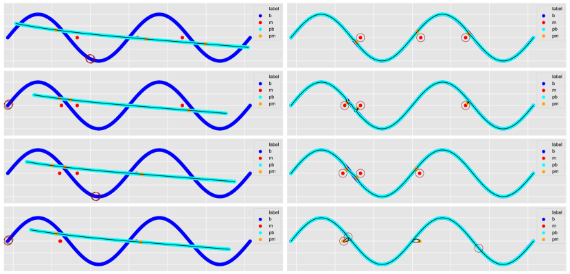
An example for this situation is shown in Figure 1, where we have used autoencoder-based UOD as described in the introduction. Each row belongs to a different dataset, while the columns belong to different autoencoders: in the first column we see the results of a regularized autoencoder and in the second column the results of a nonregularized, overfitting autoencoder. The two dimensional datasets always contain blue inliers on the sine curve (in the legend denoted by b for benign points), and three red outliers at different positions in each row (in the legend denoted by m for malign points). The cyan points (pb: predicted benign points) and the orange points (pm: predicted malign points) are the output of the autoencoder for the benign and malign data points, resp. The predicted points are all positioned on the decoder image of the latent space given by the black line. The red circles are drawn around the input points that have the three largest outlier scores. It is obvious that the regularized autoencoder fails in all four cases to approximate the benign data because it is not flexible enough. Using the reproduction error as outlier score, taking the three points with the largest outlier score as our anomalies would result in three false positives, as indicated by the red circles, and, of course, also in three false negatives. The overfitting autoencoder, on the other hand, is approximating the data much better. However, as can be seen particularly clearly in the fourth row, overfitting can result in an approximation also of the outliers which then again results in false detections. Intuitively spoken, regularization controls the “stiffness” in the approximating submanifold. Note, that in the forth row two of the randomly chosen outliers are very close to each other and look like one single point.
III-B Method Details
In the introduction section we have described a well-known popular technique of using autoencoders for UOD and in Section III-A we have discussed common problems with its application. We now propose POTATOES (Partitioning OverfiTting AuTOencoder EnSemble), a method that both improves the UOD performance of any given autoencoder, and avoids the above regularization issues.
To construct POTATOES, we first have to determine how large a cluster of outlier points can be for those points to still be considered outliers. If we have a single isolated point, this should clearly be considered an outlier. Two points being near each other but together isolated from the rest of the dataset, might still be considered both outliers. But what is the maximum size of an outlier cluster? This can only be answered by a domain expert. Thus, it should be left as a configuration parameter. Once the value of is determined, the dataset of size is partitioned into equally sized parts. If divides , each part has size , otherwise their sizes will differ by at most one. Recall the definition of a partition of a set: the collection of sets is a partition of if:
| (1) | ||||
| (2) |
Note, that with this partition, for each outlier cluster there will be at least one such that .
Next, choose an autoencoder model that is capable of overfitting. Then create copies of this autoencoder and overfit each of them to another partition, i.e. overfit to . This will result in submanifolds .
An example is provided in Figure 2. Here we choose , which means the displayed dataset has one outlier cluster containing two outliers. The data is cut into three partitions, depicted by the three colors red, green, and blue. The fitting of three belonging autoencoders results in three pertinent submanifolds.
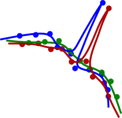
We see that each inlier has a very short distance to any of the submanifolds. This is because each inlier has in its close neighborhood far more than three other datapoints so it is very likely that each submanifold gets close to it. However, for the outliers the situation is different: since there are less data points in the outlier cluster than there are partitions, there will be at least one partition that doesn’t contain a member of the outlier cluster and thus not all submanifolds will get near the outlier cluster and thus each outlier will have at least one submanifold to which the distance is large.
This leads to the construction of the outlier score for POTATOES: Let be the reconstruction error of computed by the autoencoder . Then for each point , the POTATOES outlier score function is defined as:
| (3) |
Note, that with POTATOES it is not necessary to think about any of those methods that try to fight overfitting just the right amount, such as regularization parameters, the right choice for early stopping, or constraining the model complexity. We just have to overfit.
Moreover, As will be shown in the evaluation section, POTATOES significantly increases the UOD performance of the autoencoder it is based on.
Furthermore, although POTATOES consists of an ensemble of autoencoders, it is about as fast as a single autoencoder, since each ensemble member runs only on one th of the data. Of course, sometimes, overfitting takes more epochs to converge then regularized models, which then would increase the runtime of POTATOES. However, the ensemble autoencoders can be run in parallel, increasing the speed -fold.
Note, however, that this method only works if there is sufficient data available such that in each inlier region of the dataset there are data points of all the partitions located.
While the viewpoint adopted here is that of POTATOES being a method constructing a set of flexible data manifolds that are “dense” near the inliers and “sparse” at the outliers, one could also look at it as another method of performing UOD via nearest neighbors (-NNb). But keep in mind that -NNb based UOD algorithms have at best a complexity of in the size of the dataset, with quadratic complexity being more realistic, especially for higher dimensional data. POTATOES, on the other hand, has complexity only linear in .
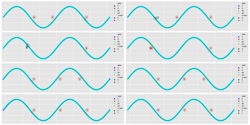
Lets apply POTATOES to a 2D example, see Figure 3. As in Figure 1, we consider a two-dimensional dataset with the inlier positioned on the sine curve and three outliers randomly chosen elsewhere. Again, each row belongs to a different dataset with different outliers. However, now the columns belong to the members of the POTATOES ensemble with . The legend shows again the same color coding in the label section as in Figure 1, but now the “in train” section has been added. This new section shows that we use crosses for the points that are contained in the partition of this autoencoder, i.e. are in its training set, and bullets for the points that are not. Clearly, most of the times, the overfitting autoencoders approximate the inliers well but don’t get to the outliers. However, in two cases, the second plot in the first row and the first plot in the second row, the autoencoder is flexible enough to also reach the outliers. Nevertheless, since in each case there is a second autoencoder that does not contain this outlier in its training set, the outlier is still recognized as such by POTATOES. This results in assigning the highest outlier score to the three outliers in each of those four cases.
IV Experimental Results
For the evaluations in this section, we used the python libraries tensorflow [18], Keras [19], and sklearn [20] for model training and inference, and seaborn [21] for the plots. The source code for the evaluations in this paper can be found at https://github.com/snetbl/potatoes. The model is evaluated for the following datasets. First, we take the well-known MNIST dataset [22], label all the images containing the zero digit as inliers, and sample from the remaining nine digits randomly some images and label them as outliers. The amount of outliers is such that in the combined set of inliers and outliers, the portion of outliers is half a percent (i.e. ). We create 50 such datasets, which have all the same inliers but differ by the randomly sampled outliers. This group will be denoted by mnist_0. This procedure is repeated, but this time the inliers are not the images with the digit zero but the images with the digit one, resulting in two groups mnist_0 and mnist_1 of 50 datasets each. Next, the MNIST dataset is replaced by the Fashion MNIST dataset [23] and the above process is repeated, which creates two further groups fmnist_0 and fmnist_1 (the Fashion MNIST class labeled 0 comprises the t-shirt/top images, the class labeled 1 the trousers). In the end, this leaves us with four groups of 50 datasets each.
The metrics used in this evaluation are the ROC area under the curve (roc_auc), the average precision (ap), optimal F1 score (of1), and precision at 20 (prec@20). The of1 metric is computed as follows: if denotes the outlier score of the point , and is the F1 score of choosing the members of as outliers, then is given by:
| (4) |
presuming that does not make any sense.
Depending on the amount of inliers, the outlier ratio of 0.005 results in a bit more than 30 outliers, which means that there are on average between three and four outliers from each of the nine outlier classes. Presuming that those are placed near each other, we expect the size of outlier clusters to be more or less of this size, and thus choose as the POTATOES ensemble size . Recall that choosing too large might deplete the inlier portions in the parts of the partition too much, so we use as a compromise.
Our choice for the original autoencoder, to which we apply the POTATOES optimization, is a vanilla deep symmetric convolutional architecture with a latent dimension of 32. The details can be found in the github repository [24] for this paper. We compare the original autoencoder with the POTATOES version of it. As described above, while we don’t use any regularization for the POTATOES ensemble, the original autoencoder does get regularized. This regularization was tuned using the knowledge of the real labels of the data, giving the regularized autoencoder an advantage that it would not have in most realistic situations, since labels are usually not available.
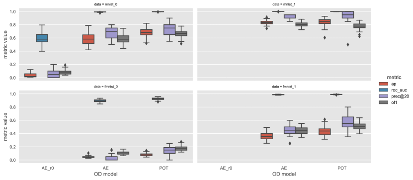
The evaluation results are shown in Figure 4 and, for the AP metric, in Table I. Here, the regularized autoencoder is abbreviated with AE and the POTATOES model with POT.
| AE | POT | |
|---|---|---|
| mnist_0 | 0.579516 | 0.682226 |
| mnist_1 | 0.836213 | 0.844658 |
| fmnist_0 | 0.044366 | 0.083286 |
| fmnist_1 | 0.359578 | 0.434675 |
We also ran evaluations for the unregularized version AE_r0 of AE. The results for AE_r0 are only shown for the mnist_0 dataset, and, because of its poor performance, has been excluded in further evaluations. Those values clearly show the potential of POTATOES. To see whether the improvements are actually significant, we have conducted paired t-tests for the AP metric. For the application of a paired t-test the following conditions have to be satisfied: Let be a group of datasets on which we compare the two models. Further, let be the AP values of POTATOES and the regularized autoencoder on the dataset , resp. Then the differences have to be (i) independent and identically distributed and (ii) samples from a normal distribution. The differences are clearly independent in each of our four dataset groups since the samplings of the outliers in the creation of the datasets are independent. Next, to check for normality, both the Shapiro-Wilk and the Kolmogorov-Smirnov test are applied. Figure 5 shows the histograms of the differences for the four groups of datasets.
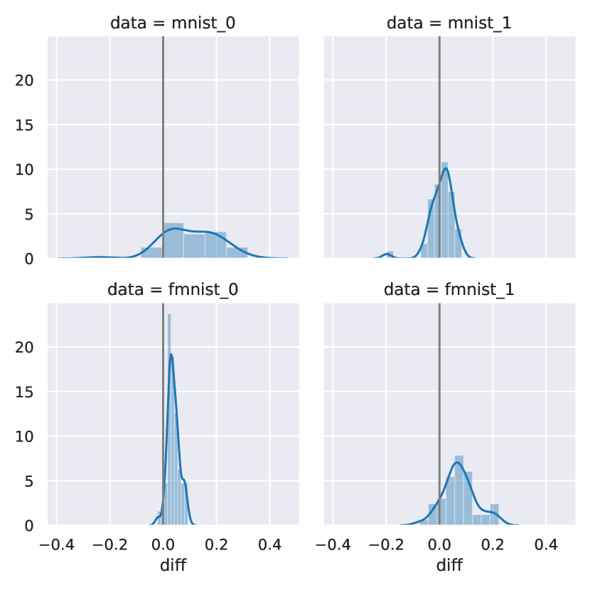
Neither Shapiro-Wilk nor Kolmogorov-Smirnov reject the null hypothesis of normality for any of these four cases, so we can apply the paired two-sample t-test. The p-values for the four groups are shown in Table II.
| mnist_0 | mnist_1 | fmnist_0 | fmnist_1 | |
| p | 5.758e-09 | 2.746e-01 | 1.688e-16 | 3.489e-11 |
Apart from the mnist_1 datasets, POTATOES always performs significantly better than its autoencoder of the same architecture.
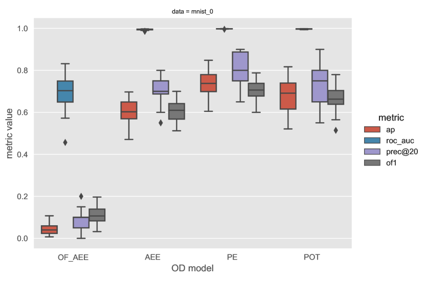
We now turn to a closer investigation of the effect of the partitioning of the training data. For this, we investigate how an overfitting ensemble of autoencoders without partitioning would perform. I.e. we keep all the parameters of POTATOES, the autoencoder architecture, zero regularization, the ensemble size of five, and the aggregation of the outlier scores of the five ensemble member models by the max function. The only difference is that each member of the ensemble is fitted on the full dataset and not just on an element of a partition; this model is abbreviated by OF_AEE. Furthermore, we include the investigation of an ensemble of regularized autoencoders without partitioning, abbreviated to AEE. Again, we use the same basic autoencoder architecture as above. The only difference between OF_AEE and AEE is the amount of regularization. Finally, we also consider an ensemble of five copies of the POTATOES model (i.e. an “ensemble of ensembles”), referred to as PE.
In this comparison, 30 datasets from mnist_0 have been used. The results are shown in Figure 6.
| AEE-POT | POT-PE | |
| p | 6.855e-6 | 5.044e-4 |
First, we clearly see that the overfitting autoencoders ensemble is not performing well, underlining that partitioning is crucial. As far as the other models are concerned, the plot suggests a ranking of the POTATOES ensemble coming first, followed by POTATOES, and the ensemble of regularized autoencoders being third. For the investigations of significance the metric AP has again been singled out. As before, neither Shapiro-Wilk nor Kolmogorov-Smirnov object to the assumption that the paired differences between the AP values are normal, so the paired two-sample t-test can be applied. Table III displays the belonging p-values: AEE-POT is for the comparison between the models AEE and POTATOES, and POT-PE is the comparison between POTATOES and PE. The values show that the ranking is significant.
V Conclusion
In this paper we have introduced POTATOES, a new method for autoencoder-based unsupervised outlier detection: For any given autoencoder architecture, it avoids the time consuming search for the optimal neural network regularization while still providing competitive UOD performance. In experiments we have shown that it outperforms the regularized version of this original autoencoder architecture, even if this regularization has been tuned using the knowledge of the true outlier labels, which is usually not available in practice. POTATOES doesn’t use those labels because it doesn’t have to tune regularization. The only conditions for its successful application are (i) that the original autoencoder is capable of overfitting the dataset when its regularization is removed and (ii) that the dataset is large enough so that each member of the partition contains sufficient inliers such that each autoencoder can still approximate any region occupied by inliers.
Furthermore, being an ensemble of independent autoencoders, POTATOES can be parallelized.
Finally, we also noted that the basic underlying idea is a rather general one of improving submanifold distance based UOD methods which need some tuning of their “manifold stiffness”. As such, it is not restricted to autoencoders and is expected to work with other submanifold learning methods, too.
References
- [1] Schölkopf, Bernhard, Alexander Smola, and Klaus-Robert Müller. ”Nonlinear component analysis as a kernel eigenvalue problem.” Neural computation 10.5 (1998): 1299-1319.
- [2] Goodfellow, Ian, Yoshua Bengio, and Aaron Courville. Deep learning. MIT press, 2016.
- [3] Cayton, Lawrence. ”Algorithms for manifold learning.” Univ. of California at San Diego Tech. Rep 12.1-17 (2005): 1.
- [4] Chalapathy, Raghavendra, and Sanjay Chawla. ”Deep learning for anomaly detection: A survey.” arXiv preprint arXiv:1901.03407 (2019).
- [5] Hodge, Victoria, and Jim Austin. ”A survey of outlier detection methodologies.” Artificial intelligence review 22.2 (2004): 85-126.
- [6] Chandola, Varun, Arindam Banerjee, and Vipin Kumar. ”Outlier detection: A survey.” ACM Computing Surveys 14 (2007): 15.
- [7] Zimek, Arthur, Erich Schubert, and Hans‐Peter Kriegel. ”A survey on unsupervised outlier detection in high‐dimensional numerical data.” Statistical Analysis and Data Mining: The ASA Data Science Journal 5.5 (2012): 363-387.
- [8] Domingues, Rémi, et al. ”A comparative evaluation of outlier detection algorithms: Experiments and analyses.” Pattern Recognition 74 (2018): 406-421.
- [9] Kwon, Donghwoon, et al. ”A survey of deep learning-based network anomaly detection.” Cluster Computing (2019): 1-13.
- [10] Schölkopf, Bernhard, Alexander J. Smola, and Francis Bach. Learning with kernels: support vector machines, regularization, optimization, and beyond. MIT press, 2002.
- [11] Perdisci, Roberto, Guofei Gu, and Wenke Lee. ”Using an ensemble of one-class svm classifiers to harden payload-based anomaly detection systems.” Sixth International Conference on Data Mining (ICDM’06). IEEE, 2006.
- [12] Liu, Fei Tony, Kai Ming Ting, and Zhi-Hua Zhou. ”Isolation forest.” 2008 Eighth IEEE International Conference on Data Mining. IEEE, 2008.
- [13] Chen, Jinghui, et al. ”Outlier detection with autoencoder ensembles.” Proceedings of the 2017 SIAM international conference on data mining. Society for Industrial and Applied Mathematics, 2017.
- [14] Mirsky, Yisroel, et al. ”Kitsune: an ensemble of autoencoders for online network intrusion detection.” arXiv preprint arXiv:1802.09089 (2018).
- [15] Khan, Shehroz S., and Babak Taati. ”Detecting unseen falls from wearable devices using channel-wise ensemble of autoencoders.” Expert Systems with Applications 87 (2017): 280-290.
- [16] Lu, Yaping, et al. ”Feature ensemble learning based on sparse autoencoders for image classification.” 2014 International Joint Conference on Neural Networks (IJCNN). IEEE, 2014.
- [17] Qi, Yumei, et al. ”Stacked sparse autoencoder-based deep network for fault diagnosis of rotating machinery.” Ieee Access 5 (2017): 15066-15079.
- [18] Abadi, Martín, et al. ”Tensorflow: A system for large-scale machine learning.” 12th USENIX symposium on operating systems design and implementation (OSDI 16). 2016.
- [19] Chollet, François. ”Keras: The python deep learning library.” ascl (2018): ascl-1806.
- [20] Pedregosa, Fabian, et al. ”Scikit-learn: Machine learning in Python.” the Journal of machine Learning research 12 (2011): 2825-2830.
- [21] Waskom, Michael, et al. ”Seaborn: statistical data visualization.” URL: https://seaborn. pydata. org/(visited on 2017-05-15) (2014).
- [22] LeCun, Yann, et al. ”Gradient-based learning applied to document recognition.” Proceedings of the IEEE 86.11 (1998): 2278-2324.
- [23] Xiao, Han, Kashif Rasul, and Roland Vollgraf. ”Fashion-mnist: a novel image dataset for benchmarking machine learning algorithms.” arXiv preprint arXiv:1708.07747 (2017).
- [24] Lorbeer, Boris. ”snetbl/potatoes”, GitHub repository, URL: https://github.com/snetbl/potatoes.