Matched Queues with Matching Batch Pair $(m,n)$

Abstract

In this paper, we develop the matrix-analytic method to discuss an interesting but challenging bilateral stochastic matching problem: A matched queue with matching batch pair $(m,n)$ and two types of impatient customers, where the two types of customers arrive according to two independent Poisson processes. Once $m$ A-customers and $n$ B-customers are matched as a group, the $m+n$ customers immediately leave the system. We show that this matched queue can be expressed as a novel bidirectional level-dependent quasi-birth-and-death (QBD) process whose analysis has its own interests, and specifically, computing the maximal non-positive inverse matrices of bidirectional infinite sizes by using the RG-factorizations. Based on this, we can provide an effective matrix-analytic method to deal with this matched queue, including the system stability, the average stationary queue lengths, the average sojourn times, and the departure process. We believe that the methodology and results developed in this paper can be applicable to studying more general matched queueing systems, which are widely encountered in many practical areas.

Keywords: Matched Queue; impatient customer; QBD process; RG-factorization; Markovian arrival process with marked transitions (MMAP); phase-type (PH) distribution.

1 Introduction

In this paper, we consider an interesting but challenging matched queue with matching batch pair $(m,n)$ and two types (i.e., types A and B) of impatient customers, where $m$ A-customers and $n$ B-customers are matched as a group and the $m+n$ customers leave the system immediately. To our best knowledge, this paper is the first to study the more general matched queue due to the matching batch pair $(m,n)$. It is worthwhile to note that the matching batch pair $(m,n)$ makes not only the model more suitable for many practically matching needs but also our Markov modeling and analysis more challenging. We show that this matched queue can be expressed as a level-dependent QBD process with bidirectional infinite levels, and thus develop some new theory of level-dependent QBD processes with bidirectional infinite levels, such as the system stability, the stationary probability vectors, the sojourn times, the first passage times, and the departure processes through dealing with the matrices of bidirectional infinite sizes by using the RG-factorizations given in Li [48]. Based on this, we can provide a detailed analysis for this matched queue, including the system stability, the average stationary queue lengths, the average sojourn times, and the departure process. Also, we can further develop some effective algorithms for analyzing the performance measures of this matched system.

So far, more and more matching problems (e.g., the double-ended queues, the matched queues, and more generally, the fork-join queues) have been widely encountered in many different practical areas, for example, sharing economy, ridesharing platform, bilateral market, organ transplantation, assembly systems, taxi services, seaport and airport, and so on. Important research examples include: Organ transplantation by Zenios [80], Boxma et al. [11], Stanford et al. [66], and Elalouf et al. [27]; taxi services by Giveen [29, 30], Kashyap [41, 42, 43], Bhat [9], Baik et al. [6], Shi and Lian [64], and Zhang et al. [81]; baggage claim by Browne et al. [15]; sharing economy by Cheng [19], Sutherland and Jarrahi [68], and Benjaafar and Hu [8]; assembly systems by Hopp and Simon [36], Som et al. [65], and Ramachandran and Delen [60]; health care by Pandey and Gangeshwer [57]; multimedia synchronization by Steinmetz [67] and Parthasarathy et al. [58]; and so forth.

Besides these, in recent years, an emerging hot research topic of matched queues has been focused on ridesharing platform. Many ridesharing companies spring up as a result of rapid development of mobile networks, smart phones and location technologies, for example, Uber in transportation, Airbnb in housing, Eatwith in eating, Rent the Runway in dressing, and so on. Readers may refer to, such as Azevedo and Weyl [5], Duenyas et al. [26], Hu and Zhou [37], Banerjee and Johari [7] and Braverman et al. [12]. Obviously, the matched queues have become useful and necessary in both theory research and real applications of ridesharing platforms with various different services.

Now, we summarize the literature of matched queues from three different aspects of matching batch pair $(m,n)$ as follows:

The matching batch pair $(1,1)$. Early research of matching queues first focused on some simple double-ended (or matched) systems with matching batch pair $(1,1)$. Also, the matched queues with matching batch pair $(1,1)$ have attracted numerous researchers’ attention since a pioneering work by Kendall [44], and crucially, some effective methodologies and available results have been developed from multiple research perspectives listed below.

The Markov process: Such a process was the first effective method employed in early research of matched queues. For a simple matched queue, Sasieni [62], Giveen [29] and Dobbie [25] established the Chapman-Kolmogorov forward differential-difference equations, in which the customers’ impatient behavior was introduced to guarantee the system stability. Since then, the Markov process analysis of matched queues was further developed from two different research lines:

(a) A finite state space. When the two waiting rooms of the matched queue are both finite, the Markov process is established on a finite state space. In this case, Jain [38] and Kashyap [41, 42, 43] applied the supplementary variable method to be able to deal with the matched queue with a Poisson arrival process and a renewal arrival process, and specifically, Takahashi et al. [69] considered the matched queue with a Poisson arrival process and a PH-renewal arrival process. In addition, Sharma and Nair[63] used the matrix theory to analyze the transient behavior of a Markovian matched queue. Chai et al. [18] considered a batch matching queueing system with impatient servers and bounded rational customers, and each server serves the customers in batches with finite service capacity.

(b) An infinite state space. When the two waiting rooms of the matched queue are both infinite, the Markov process is set up with a bidirectional infinite state space. In general, it is always difficult to analyze such a Markov process on a bidirectional infinite state space. Latouche [46] applied the matrix-geometric solution to analyze several bilateral matched queues with paired input. Conolly et al. [20] applied the Laplace transform to discuss the time-dependent performance measures of the matched queue with state-dependent impatience. Di Crescenzo et al. [22, 23] discussed the transient and stationary probabilities of a time-nonhomogeneous matched queue with catastrophes and repairs. Diamant and Baron [24] analyzed a matched queue with priority and impatient customers.

The fluid and diffusion approximations: In a matched queue, if the arrivals of A- and B-customers are both general renewal processes, then the fluid and diffusion approximations become an effective (but approximative) method. Jain [40] applied the diffusion approximation to discuss the G${}^{\text{X}}$/G${}^{\text{Y}}$/1 matched queue. Di Crescenzo et al. [22, 23] discussed a matched queue by means of a jump-diffusion approximation. Liu et al. [53] discussed some diffusion models for the matched queues with renewal arrival processes. Büke and Chen [17] applied the fluid and diffusion approximations to study the probabilistic matching systems. Liu [52] used the diffusion approximation to analyze the matched queues with reneging in heavy traffic.

Other effective methods: Adan et al. [1, 2] and Visschers et al. [71] discussed the matched systems with multi-type jobs and multi-type servers by using the product solution of queueing networks. Kim et al. [45] provided a simulation model to analyze a more general matched queue. Jain [39] proposed a sample path analysis for studying the matched queue with time-dependent rates. Afèche et al. [3] applied the level-cross method to discuss the batch matched queue with abandonment. Wu and He [72] used the multi-layer Markov modulated fluid flow (MMFF) processes to deal with a double-sided queueing model with marked Markovian arrival processes and finite discrete abandonment times.

Control of matched queues: Hlynka and Sheahan [35] analyzed the control rates in a matched queue with two Poisson inputs. Gurvich and Ward [31] discussed dynamic control of the matching queues. Büke and Chen [16] studied stabilizing admission control policies for the probabilistic matching systems. Lee et al. [47] studied optimal control of a time-varying double-ended production queueing system.

The matching batch pair $(1,n)$. As a key generalization, Xu et al. [73] first discussed a matched queue with matching batch pair $(1,n)$, in which for the two waiting rooms, one is finite while another is infinite. Under two Poisson inputs and a PH service time distribution, they applied the matrix-geometric solution to obtain the stability condition of the system, and to study the stationary queue lengths for the both classes of customers. Since then, further research includes Xu and He [74, 75]. Yuan [78] applied Markov chains of M/G/1 type to consider a matched queue with matching batch pair $(1,n)$ and under two Poisson inputs and a general service time distribution. Li and Cao [49] discussed the matched queue with matching batch pair $(1,n)$ and under two batch Markovian arrival processes (BMAPs) and a general service time distribution.

The matching batch pair $(m,n)$. To our best knowledge, this paper is the first to study the matched queues with matching batch pair $(m,n)$, where the two waiting rooms are both infinite. We express this matched queue as a level-dependent QBD process with bidirectional infinite levels, and apply the RG-factorizations given in Li [48] to obtain the average stationary queue lengths, the average sojourn times, and the departure process. Note that Liu et al. [51] is a closely related work to study such matched queues whose corresponding Markov processes are block-structured and level-dependent. Different from Liu et al. [51], the matching batch pair $(m,n)$ makes the Markov block structure of bidirectional infinity sizes more challenging. In addition, we develop the matrix-analytic method to study the average sojourn time and the departure process through setting up a new PH distribution of bidirectional infinity sizes and a new Markovian arrival process with marked transitions (MMAP) of bidirectional infinity sizes, respectively.

In what follows, it is necessary to discuss some random features of the matched queues from the theory of Markov processes.

On the one hand, the matched queues are a type of interesting and classic systems in early research of queuing systems, but their available methodologies and results are fewer than those developed for other types of classic queueing systems, for example, processor-sharing queues (Yashkov [76] and Yashkov and Yashkov [77]), and retrial queues (Falin and Templeton [28] and Artalejo and Gómez-Corral [4]). In fact, the matrix-analytic method (based on the level-dependent Markov processes) have been applied to analysis of the retrial queues or the processor-sharing queues, e.g., See Chapter 5 in Artalejo and Gómez-Corral [4] and Chapter 7 in Li [48]. On the other hand, it is relatively difficult to discuss the queues with impatient customers (even though the impatient times are exponential). Note that the general impatient times can make the embedded Markov process analysis of the queue very complicated and even impossible except for using the fluid and diffusion approximations under an approximate goal, e.g., see Boots and Tijms [10], Zeltyn and Mandelbaum [79], and Puha and Ward [59]. Furthermore, the customers’ impatient behavior greatly complicates the analysis of matched queues due to the level-dependent structure of their corresponding Markov process with bidirectional infinite levels. Thus, the matrix-analytic method needs to further be developed through applying the Markov process with bidirectional infinite levels to dealing with the matched queueing example with matching batch pair $(m,n)$.

In the study of matched queues, the matching batch pair $(m,n)$ greatly complicates how to concretely write the infinitesimal generator of the level-dependent QBD process with bidirectional infinite levels. Also, the matching batch pair $(m,n)$ convincingly motivate us to develop the matrix-analytic method of matched queues, which can be applied to dealing with many practical matching problems. For the matrix-analytic method to the study of matched queues, the level-dependent Markov processes are a key and their analysis is based on the RG-factorizations given in Li [48]. Thus, the RG-factorizations play a key role in the study of matched queues. By using the RG-factorizations, we can further develop some effective algorithms (also see some algorithmic research by Bright and Taylor [13, 14], Takine [70] and Liu et al. [51]) to be able to numerically analyze performance measures of the matched queues. Although some results given in this paper are regarded as superficially coming from Chapter 2 of Li [48], the level-dependent block structure leads to some new advances in the matrix-analytic method of matched queues, including the level-dependent Markov processes with bidirectional infinite levels, the maximal non-positive inverse matrices of bidirectional infinite sizes, the sojourn times of bidirectional infinite sizes, the departure processes of bidirectional infinite sizes, and so forth.

The Markovian arrival process (MAP) is a useful mathematical tool, for example, for describing bursty traffic and dependent arrivals in many real systems, such as computer and communication networks, manufacturing systems, transportation networks and so on. Readers may refer to, such as Chapter 5 in Neuts [56], Lucantoni [54], Chapter 1 in [48] and references therein. Further, He [32] and He and Neuts [33] introduced the MMAP, which is useful in modeling input (or departure) processes of stochastic systems with several types of items (e.g., customers or orders). In this paper, we use the MMAP of bidirectional infinity sizes to study the departure process with three types of customers in the matched queue with matching batch pair $(m,n)$.

Based on the above analysis, we summarize the main contributions of this paper as follows:

• We describe and analyze a more general matched queue with matching batch pair $(m,n)$, where $m$ A-customers and $n$ B-customers are matched as a group and the $\left(m+n\right)$ customers leave the system immediately. Such a matched queue can widely be used to study many practically matching problems, for example, sharing economy, ridesharing platform, bilateral market, organ transplantation, taxi services, assembly systems, and so on.

• We express the matched queue with matching batch pair $(m,n)$ as a level-dependent QBD process with bidirectional infinite levels. Thus, we develop the matrix-analytic method by means of the level-dependent QBD processes with bidirectional infinite levels, such as the system stability, the stationary probability vectors, the sojourn times, the first passage times, and the departure processes. A key of our method is based on applying the RG-factorizations given in Li [48] to dealing with the maximal non-positive inverse matrices of bidirectional infinite sizes.

• We provide a detailed analysis for the matched queue with matching batch pair $(m,n)$, including the system stability, the average stationary queue lengths, the average sojourn times, and the departure process. Specifically, the average sojourn times are given a better upper bound by using a new phase-type distribution of bidirectional infinity sizes, and the departure process with three types of customers is established in terms of the MMAP of bidirectional infinity sizes. Also, some numerical examples are used to indicate our theoretical results.

The structure of this paper is organized as follows. Section 2 describes a more general matched queue with matching batch pair $(m,n)$ and two types of impatient customers. Section 3 expresses this matched queue as a level-dependent QBD process with bidirectional infinite levels, and provides the stability condition of the system. Section 4 studies the stationary probability vector of the QBD process with bidirectional infinite levels, and thus computes the average stationary queue length of any A- or B-customer. Section 5 computes the average sojourn time of any A- or B-customer by using three different techniques: The Little’s formula, a probabilistic calculation, and an upper bound, respectively. Section 6 uses the MMAP of bidirectional infinite sizes to discuss the departure process with three types of customers. Finally, some concluding remarks are given in Section 7.

2 Model Description

In this section, we describe a more general matched queue with matching batch pair $(m,n)$ and two types of impatient customers, and also introduce operational mechanism, system parameters and basic notation.

In the matched queue with matching batch pair $(m,n)$, $m$ A-customers and $n$ B-customers are matched as a group which leaves the system immediately once such a matching is successful, and also the customers’ impatient behavior is used to guarantee the stability of the system. Figure 1 provides a physical illustration for such a matched queue.

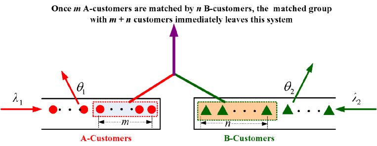
Figure 1: A physical illustration of the matched queue

Now, we provide a more detailed description for the matched queue as follows:

(1) Arrival processes. The A- and B-customers arrive at the queueing system according to two Poisson processes with rates $\lambda_{1}$ and $\lambda_{2}$, respectively.

(2) Matching processes. When $m$ customers of type A and $n$ customers of type B are present, there is a match and these $m+n$ customers immiediately leave the system for $m,n\geq 1$. Customers for whom there is not yet a match must wait. Their matching process follows a First-Come-First-Match discipline. We assume that the two waiting spaces of A- and B-customers are both infinite.

(3) Impatient behavior. If an A-customer (resp. a B-customer) stays at the queueing system for a long time, then she will have some impatient behavior. We assume that the impatient time of an A-customer (resp. a B-customer) is exponentially distributed with impatient rate $\theta_{1}$ (resp. $\theta_{2}$) for $\theta_{1},\theta_{2}>0$.

We assume that all the random variables defined above are independent of each other.

Remark 1.

(a) The customers’ impatient behavior given in Assumption (3) is used to ensure the stability of the matched queue.

(b) The matching discipline given in Assumption (2) indicates that more than $m$ A-customers and more than $n$ B-customers cannot simultaneously exist in their waiting spaces.

3 A QBD Process with Bidirectional Infinite Levels

In this section, we describe the matched queue with matching batch pair $(m,n)$ as a new bidirectional level-dependent QBD process to express , and obtain a sufficient condition under which this matched queue is stable.

We denote by $N_{1}\left(t\right)$ and $N_{2}\left(t\right)$ the numbers of A- and B-customers in the matched queue at time $t\geq 0$, respectively. Then the matched queue with matching batch pair $(m,n)$ is related to a two-dimensional Markov process $\left\{\left(N_{1}\left(t\right),N_{2}\left(t\right)\right),\text{ }t\geq 0\right\}$. Note that once $m$ A-customers and $n$ B-customers are matched as a group, the $m+n$ customers immediately leave the queueing system, thus more than $m$ A-customers and more than $n$ B-customers cannot simultaneously exist in their waiting spaces. Based on this, the state space of the Markov process $\left\{\left(N_{1}\left(t\right),N_{2}\left(t\right)\right),\text{ }t\geq 0\right\}$ is given by

$$\Omega= \left\{\left(i,j\right):0\leq i\leq m-1,0\leq j\leq n-1\right\}\cup\left\{\left(i,j\right):i\geq m,0\leq j\leq n-1\right\}$$

$$\cup\left\{\left(i,j\right):0\leq i\leq m-1,j\geq n\right\}.$$

In this case, we write

$$\text{Level }0= \left\{\left(0,0\right),\left(0,1\right),\ldots,\left(0,n-1\right);\left(1,0\right),\text{ }\left(1,1\right),,\ldots,\text{\ }\left(1,n-1\right);\right.$$ (1)

$$\left.\ldots;\text{\ }\left(m-1,0\right),\text{\ }\left(m-1,1\right),\ldots,\text{\ }\left(m-1,n-1\right)\right\},$$

for $k\geq 1,$

$$\text{Level }k= \left\{\left(km,0\right),\left(km,1\right),\ldots,\left(km,n-1\right);\left(km+1,0\right),\text{ }\left(km+1,1\right),\ldots,\left(km+1,n-1\right);\right.$$ (2)

$$\left.\ldots;\text{\ }\left(km+\left(m-1\right),0\right),\left(km+\left(m-1\right),1\right),\ldots,\left(km+\left(m-1\right),n-1\right)\right\},$$

and $l\leq-1,$

$$\text{Level }l= \left\{\left(m-1,\left(-l\right)n+n-1\right),\left(m-2,\left(-l\right)n+n-1\right),\ldots,\left(0,\left(-l\right)n+n-1\right);\ldots;\right.$$

$$\left(m-1,\left(-l\right)n+1\right),\left(m-2,\left(-l\right)n+1\right),\ldots,\left(0,\left(-l\right)n+1\right);$$

$$\left.\left(m-1,\left(-l\right)n\right),\left(m-2,\left(-l\right)n\right),\ldots,\left(0,\left(-l\right)n\right)\right\},$$ (3)

Therefore, we have

$$\Omega=\bigcup\limits_{k=-\infty}^{\infty}\text{Level }k.$$

Example one: As an illustrated example, we take $m=2$ and $n=3$. In this case, the state transition relations of Markov process $\left\{\left(N_{1}\left(t\right),N_{2}\left(t\right)\right),\text{ }t\geq 0\right\}$ are depicted in Figure 2. Also, we observe that each level is a state set formed by many states in a rectangle (i.e., multiple state lines).

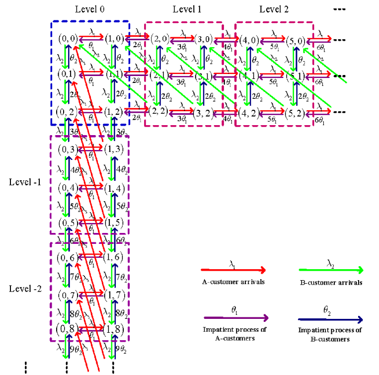
Figure 2: The state transition relations of the bilateral QBD process

From Levels $k$ for $-\infty<k<\infty$ or Figure 2, it is easy to see that the Markov process $\{(N_{1}\left(t\right),N_{2}\left(t\right)),$ $t\geq 0\}$ is a new level-dependent QBD process with bidirectional infinite levels whose infinitesimal generator is given by

$$Q=\left(\begin{array}[c]{ccccccccccc}\ddots&\ddots&\ddots&&&&&&&&\\ &B_{0}^{\left(-3\right)}&B_{1}^{\left(-3\right)}&B_{2}^{\left(-3\right)}&&&&&&&\\ &&B_{0}^{\left(-2\right)}&B_{1}^{\left(-2\right)}&B_{2}^{\left(-2\right)}&&&&&&\\ &&&B_{0}^{\left(-1\right)}&B_{1}^{\left(-1\right)}&\framebox{$B_{2}^{\left(-1\right)}$}&&&&&\\ &&&&\framebox{$B_{0}^{\left(0\right)}$}&C&\framebox{$A_{0}^{\left(0\right)}$}&&&&\\ &&&&&\framebox{$A_{2}^{\left(1\right)}$}&A_{1}^{\left(1\right)}&A_{0}^{\left(1\right)}&&&\\ &&&&&&A_{2}^{\left(2\right)}&A_{1}^{\left(2\right)}&A_{0}^{\left(2\right)}&&\\ &&&&&&&A_{2}^{\left(3\right)}&A_{1}^{\left(3\right)}&A_{0}^{\left(3\right)}&\\ &&&&&&&&\ddots&\ddots&\ddots\end{array}\right),$$ (4)

where, for $k\geq 0,$

$$\text{Level }k= \left\{\left(km,0\right),\left(km,1\right),\ldots,\left(km,n-1\right);\left(km+1,0\right),\text{ }\left(km+1,1\right),\ldots,\left(km+1,n-1\right);\right.$$

$$\left.\ldots;\text{\ }\left(km+\left(m-1\right),0\right),\left(km+\left(m-1\right),1\right),\ldots,\left(km+\left(m-1\right),n-1\right)\right\},$$

we have

$$C=\left(\begin{array}[c]{ccccc}A_{1,1}^{\left(0\right)}&A_{2,1}&&&\\ A_{3,1}^{\left(0\right)}&A_{1,2}^{\left(0\right)}&A_{2,2}&&\\ &\ddots&\ddots&\ddots&\\ &&A_{3,m-2}^{\left(0\right)}&A_{1,m-1}^{\left(0\right)}&A_{2,m-1}\\ &&&A_{3,m-1}^{\left(0\right)}&A_{1,m}^{\left(0\right)}\end{array}\right)_{mn\times mn},\text{ \ }$$

$$A_{1,i}^{\left(0\right)}=\left(\begin{array}[c]{ccccc}a_{1,i}^{\left(0,1\right)}&\lambda_{2}&&&\\ \theta_{2}&a_{1,i}^{\left(0,2\right)}&\lambda_{2}&&\\ &\ddots&\ddots&\ddots&\\ &&\left(n-2\right)\theta_{2}&a_{1,i}^{\left(0,n-1\right)}&\lambda_{2}\\ &&&\left(n-1\right)\theta_{2}&a_{1,i}^{\left(0,n\right)}\end{array}\right)_{n\times n},\text{ }1\leq i\leq m,$$

$$a_{1,i}^{\left(0,r\right)}=-\left(\lambda_{1}+\lambda_{2}+\left(r-1\right)\theta_{2}+\left(i-1\right)\theta_{1}\right),\text{ }1\leq r\leq n;$$

$$A_{1}^{\left(k\right)}=\left(\begin{array}[c]{ccccc}A_{1,1}^{\left(k\right)}&A_{2,1}&&&\\ A_{3,1}^{\left(k\right)}&A_{1,2}^{\left(k\right)}&A_{2,2}&&\\ &\ddots&\ddots&\ddots&\\ &&A_{3,m-2}^{\left(k\right)}&A_{1,m-1}^{\left(k\right)}&A_{2,m-1}\\ &&&A_{3,m-1}^{\left(k\right)}&A_{1,m}^{\left(k\right)}\end{array}\right)_{mn\times mn},\text{ \ }k\geq 0,$$

$$A_{1,i}^{\left(k\right)}=\left(\begin{array}[c]{ccccc}a_{1,i}^{\left(k,1\right)}&\lambda_{2}&&&\\ \theta_{2}&a_{1,i}^{\left(k,2\right)}&\lambda_{2}&&\\ &\ddots&\ddots&\ddots&\\ &&\left(n-2\right)\theta_{2}&a_{1,i}^{\left(k,n-1\right)}&\lambda_{2}\\ &&&\left(n-1\right)\theta_{2}&a_{1,i}^{\left(k,n\right)}\end{array}\right)_{n\times n},\text{ }1\leq i\leq m,$$

$$a_{1,i}^{\left(k,r\right)}=-\left(\lambda_{1}+\lambda_{2}+\left(r-1\right)\theta_{2}+\left(km+i-1\right)\theta_{1}\right),\text{ }1\leq r\leq n,$$

$$A_{2,i}=\left(\begin{array}[c]{cccc}\lambda_{1}&&&\\ &\lambda_{1}&&\\ &&\ddots&\\ &&&\lambda_{1}\end{array}\right)_{n\times n},1\leq i\leq m-1,$$

$$A_{3,i}^{\left(k\right)}=\left(\begin{array}[c]{cccc}\left(km+i\right)\theta_{1}&&&\\ &\left(km+i\right)\theta_{1}&&\\ &&\ddots&\\ &&&\left(km+i\right)\theta_{1}\end{array}\right)_{n\times n},\text{ }1\leq i\leq m-1;$$

note that $A_{0}^{\left(k\right)}$ is a transition rate matrix from Level $k$ to Level $k+1$, we obtain

$$A_{0}^{\left(k\right)}=\left(\begin{array}[c]{cc}{\huge 0}_{\left[\left(m-1\right)n\right]\times n}&{\huge 0}_{\left[\left(m-1\right)n\right]\times\left[\left(m-1\right)n\right]}\\ \text{ }\left.\begin{array}[c]{ccc}\lambda_{1}&&\\ &\ddots&\\ &&\lambda_{1}\end{array}\right\}n\times n&{\huge 0}_{n\times\left[\left(m-1\right)n\right]}\end{array}\right)_{mn\times mn},\text{\ }k\geq 0;$$

since $A_{2}^{\left(k\right)}$ is a transition rate matrix from Level $k$ to Level $k-1$, we obtain

$$A_{2}^{\left(k\right)}=\left(\begin{array}[c]{ccc}\left.\begin{array}[c]{ccc}0&&\\ &\ddots&\\ \lambda_{2}&&0\end{array}\right\}n\times n&\cdots&\left.\begin{array}[c]{ccc}km\theta_{1}&&\\ &\ddots&\\ &&km\theta_{1}\end{array}\right\}n\times n\\ &\ddots&\vdots\\ &&\left.\begin{array}[c]{ccc}\text{ \ }0\text{ \ }&\text{ \ \ \ }&\text{ \ \ \ \ \ \ \ }\\ \text{ \ }&\ddots&\\ \lambda_{2}&&0\end{array}\right\}n\times n\end{array}\right)_{mn\times mn},\text{\ }k\geq 1.$$

For $l\leq-1,$

$$\text{Level }l= \left\{\left(m-1,\left(-l\right)n+n-1\right),\left(m-2,\left(-l\right)n+n-1\right),\ldots,\left(0,\left(-l\right)n+n-1\right);\ldots;\right.$$

$$\left(m-1,\left(-l\right)n+1\right),\left(m-2,\left(-l\right)n+1\right),\ldots,\left(0,\left(-l\right)n+1\right);$$

$$\left.\left(m-1,\left(-l\right)n\right),\left(m-2,\left(-l\right)n\right),\ldots,\left(0,\left(-l\right)n\right)\right\},$$

we have

$$B_{1}^{\left(l\right)}=\left(\begin{array}[c]{ccccc}B_{1,1}^{\left(l\right)}&B_{2,1}^{\left(l\right)}&&&\\ B_{3,1}&B_{1,2}^{\left(l\right)}&B_{2,2}^{\left(l\right)}&&\\ &\ddots&\ddots&\ddots&\\ &&B_{3,n-2}&B_{1,n-1}^{\left(l\right)}&B_{2,n-1}^{\left(l\right)}\\ &&&B_{3,n-1}&B_{1,n}^{\left(l\right)}\end{array}\right)_{mn\times mn},\text{ }l\leq-1,$$

$$B_{1,i}^{\left(l\right)}=\left(\begin{array}[c]{ccccc}b_{1,i}^{\left(l,1\right)}&\left(m-1\right)\theta_{1}&&&\\ \lambda_{1}&b_{1,i}^{\left(l,2\right)}&\left(m-2\right)\theta_{1}&&\\ &\ddots&\ddots&\ddots&\\ &&\lambda_{1}&b_{1,i}^{\left(l,m-1\right)}&\theta_{1}\\ &&&\lambda_{1}&b_{1,i}^{\left(l,m\right)}\end{array}\right)_{m\times m},\text{ }1\leq i\leq n,$$

$$b_{1,i}^{\left(l,r\right)}=-\left(\lambda_{1}+\lambda_{2}+\left(m-r\right)\theta_{1}+\left(-ln+n-i\right)\theta_{2}\right),\text{ }1\leq r\leq m,$$

$$B_{2,i}^{\left(l\right)}=\left(\begin{array}[c]{cccc}\left(-ln+n-i\right)\theta_{2}&&&\\ &\left(-ln+n-i\right)\theta_{2}&&\\ &&\ddots&\\ &&&\left(-ln+n-i\right)\theta_{2}\end{array}\right)_{m\times m},1\leq i\leq n-1,$$

$$B_{3,i}=\left(\begin{array}[c]{cccc}\lambda_{2}&&&\\ &\lambda_{2}&&\\ &&\ddots&\\ &&&\lambda_{2}\end{array}\right)_{m\times m},1\leq i\leq n-1;$$

note that $B_{0}^{\left(0\right)}$ is a transition rate matrix from Level $0$ to Level $-1$ while Level $0$ and Level $-1$ have a different lexicographic order, we obtain

$$B_{0}^{\left(0\right)}=\left(\begin{array}[c]{cc}{\huge 0}_{n\times\left[\left(n-1\right)m\right]}&\left.\begin{array}[c]{ccc}0&\cdots&0\\ \vdots&\ddots&\vdots\\ 0&\cdots&\lambda_{2}\end{array}\right\}n\times m\\ \vdots&\vdots\\ {\huge 0}_{n\times\left[\left(n-1\right)m\right]}&\left.\begin{array}[c]{ccc}0&\cdots&0\\ \vdots&\ddots&\vdots\\ \lambda_{2}&\cdots&0\end{array}\right\}n\times m\end{array}\right)_{mn\times mn},$$

it is easy to see that for $l\leq-1$, $B_{0}^{\left(l\right)}$ is a transition rate matrix from Level $l+1$ to Level $l$ while Level $l+1$ and Level $l$ have the same lexicographic order, we obtain

$$B_{0}^{\left(l\right)}=\left(\begin{array}[c]{cc}\text{\ }{\huge 0}_{m\times\left[\left(n-1\right)m\right]}\text{\ }&\left.\begin{array}[c]{ccc}\lambda_{2}&&\\ &\ddots&\\ &&\lambda_{2}\end{array}\right\}m\times m\\ {\huge 0}_{\left[\left(n-1\right)m\right]\times\left[\left(n-1\right)m\right]}&\text{ \ \ }{\huge 0}_{\left[\left(n-1\right)m\right]\times m}\end{array}\right)_{mn\times mn},\text{ }l\leq-1;$$

since $B_{2}^{\left(-1\right)}$ is a transition rate matrix from Level $-1$ to Level $0$ while Level $-1$ and Level $0$ have a different lexicographic order, we obtain

$$B_{2}^{\left(-1\right)}=\left(\begin{array}[c]{cccc}\left.\begin{array}[c]{ccccc}0&0&\cdots&0&\lambda_{1}\\ \vdots&\vdots&&\vdots&\vdots\\ 0&0&\cdots&0&0\\ 0&0&\cdots&0&0\end{array}\right\}m\times n&&&\\ \left.\begin{array}[c]{ccccc}0&0&\cdots&\lambda_{1}&0\\ \vdots&\vdots&&\vdots&\vdots\\ 0&0&\cdots&0&0\\ 0&0&\cdots&0&0\end{array}\right\}m\times n&&&\\ \vdots&&&\\ \left.\begin{array}[c]{ccccc}0&\lambda_{1}&\cdots&0&0\\ \vdots&\vdots&&\vdots&\vdots\\ 0&0&\cdots&0&0\\ 0&0&\cdots&0&0\end{array}\right\}m\times n&&&\\ \left.\begin{array}[c]{ccccc}\lambda_{1}&0&\cdots&0&0\\ \vdots&\vdots&&\vdots&\vdots\\ 0&0&\cdots&0&0\\ 0&0&\cdots&0&n\theta_{2}\end{array}\right\}m\times n&\left.\begin{array}[c]{cc}{\huge 0}&0\\ \vdots&\vdots\\ {\huge 0}&n\theta_{2}\\ {\huge 0}&0\end{array}\right\}m\times n&\cdots&\left.\begin{array}[c]{cc}{\huge 0}&n\theta_{2}\\ \vdots&\vdots\\ {\huge 0}&0\\ {\huge 0}&0\end{array}\right\}m\times n\end{array}\right)_{{}_{mn\times mn}},$$

observing that for $l\leq-1$, $B_{2}^{\left(l\right)}$ is a transition rate matrix from Level $l$ to Level $l+1$ while Level $l$ and Level $l+1$ have the same lexicographic order, we obtain

$$B_{2}^{\left(l\right)}=\left(\begin{array}[c]{ccc}\left.\begin{array}[c]{ccc}0&&\lambda_{1}\\ &\ddots&\\ &&0\end{array}\right\}m\times m&&\\ \vdots&\ddots&\\ \left.\begin{array}[c]{ccc}-ln\theta_{2}&&\\ &\ddots&\\ &&-ln\theta_{2}\end{array}\right\}m\times m&\cdots&\left.\begin{array}[c]{ccc}0&&\lambda_{1}\\ &\ddots&\\ &&0\end{array}\right\}m\times m\end{array}\right)_{mn\times mn},\text{ }l\leq-2,$$

Remark 2.

The element order of the state space $\Omega=\cup_{k=-\infty}^{\infty}$Level $k$ is arranged from left to right not only for the levels but also for the elements in each level. Thus, from (1), (2) and (3), it is observed the useful difference between Level $k$ for $k\geq 0$, and Level $L$ for $l\leq-1$. In this case, from considering the example in Figure 1, it is useful to observe the two special blocks for how to write the infinitesiaml generator $Q$ as follows:

$$B_{0}^{\left(0\right)}=\begin{array}[c]{cc}&\begin{array}[c]{cccccc}\left(1,5\right)&\left(0,5\right)&\left(1,4\right)&\left(0,4\right)&\left(1,3\right)&\left(0,3\right)\end{array}\\ \begin{array}[c]{c}\left(0,0\right)\\ \left(0,1\right)\\ \left(0,2\right)\\ \left(1,0\right)\\ \left(1,1\right)\\ \left(1,2\right)\end{array}&\text{Level }0\rightarrow\text{Level }-1\end{array}$$

and

$$B_{2}^{\left(-1\right)}=\begin{array}[c]{cc}&\begin{array}[c]{cccccc}\left(0,0\right)&\left(0,1\right)&\left(0,2\right)&\left(1,0\right)&\left(1,1\right)&\left(1,2\right)\end{array}\\ \begin{array}[c]{c}\left(1,5\right)\\ \left(0,5\right)\\ \left(1,4\right)\\ \left(0,4\right)\\ \left(1,3\right)\\ \left(0,3\right)\end{array}&\text{Level }-1\rightarrow\text{Level }0\end{array}.$$

Now, we discuss the stability of the QBD process $Q$ with bidirectional infinite levels. Our method is to divide the bidirectional QBD process $Q$ into two unilateral QBD processes: $Q_{A}$ and $Q_{B}$.

To analyze the matched queue with matching batch pair $(m,n)$, it is worthwhile to note that a simple relation between Levels $0$ and $-1$ is a key. From Levels $0$ and $-1$, we can divide the bidirectional QBD process $Q$ into two unilateral QBD processes: $Q_{A}$ and $Q_{B}$. Based on this, the infinitesimal generators of the two unilateral QBD processes $Q_{A}$ and $Q_{B}$ are respectively given by

$$Q_{A}=\left(\begin{array}[c]{cccccc}C+B_{0}^{\left(0\right)}&\framebox{$A_{0}^{\left(0\right)}$}&&&&\\ \framebox{$A_{2}^{\left(1\right)}$}&A_{1}^{\left(1\right)}&A_{0}^{\left(1\right)}&&&\\ &A_{2}^{\left(2\right)}&A_{1}^{\left(2\right)}&A_{0}^{\left(2\right)}&&\\ &&A_{2}^{\left(3\right)}&A_{1}^{\left(3\right)}&A_{0}^{\left(3\right)}&\\ &&&\ddots&\ddots&\ddots\end{array}\right)$$

and

$$Q_{B}=\left(\begin{array}[c]{cccccc}C+A_{0}^{\left(0\right)}&\framebox{$B_{0}^{\left(0\right)}$}&&&&\\ \framebox{$B_{2}^{\left(-1\right)}$}&B_{1}^{\left(-1\right)}&B_{0}^{\left(-1\right)}&&&\\ &B_{2}^{\left(-2\right)}&B_{1}^{\left(-2\right)}&B_{0}^{\left(-2\right)}&&\\ &&B_{2}^{\left(-3\right)}&B_{1}^{\left(-3\right)}&B_{0}^{\left(-3\right)}&\\ &&&\ddots&\ddots&\ddots\end{array}\right),$$

which can be given by the following infinitesimal generator when the levels are re-arranged in a new order $\left\{\text{Level }0,\text{Level }-1,\text{Level }-2,\ldots\right\}$ from its original order $\{\ldots,$Level $-2$, Level $-1,$Level $0\}$, seeing the above part of the infinitesimal generator $Q$ given in (4) as follows:

$$Q_{B}=\left(\begin{array}[c]{cccccc}\ddots&\ddots&\ddots&&&\\ &B_{0}^{\left(-3\right)}&B_{1}^{\left(-3\right)}&B_{2}^{\left(-3\right)}&&\\ &&B_{0}^{\left(-2\right)}&B_{1}^{\left(-2\right)}&B_{2}^{\left(-2\right)}&\\ &&&B_{0}^{\left(-1\right)}&B_{1}^{\left(-1\right)}&\framebox{$B_{2}^{\left(-1\right)}$}\\ &&&&\framebox{$B_{0}^{\left(0\right)}$}&C+A_{0}^{\left(0\right)}\end{array}\right).$$

Note that $\left[\left(C+B_{0}^{\left(0\right)}\right)+A_{0}^{\left(0\right)}\right]e=0$ for $Q_{A}$, and $\left[\left(C+A_{0}^{\left(0\right)}\right)+B_{0}^{\left(0\right)}\right]e=0$ for $Q_{B}$, where $e$ is a column vector of ones with a suitable dimension.

In the remainder of this section, we study the stability of the matched queue with matching batch pair $(m,n)$. It is easy to see that the customers’ impatient behavior plays a key role in the stability analysis.

The following theorem provides a sufficient condition under which the QBD process with bidirectional infinite levels is stable.

Theorem 1.

If $\left(\theta_{1},\theta_{2}\right)>0$, then the QBD process $Q$ with bidirectional infinite levels is irreducible and positive recurrent. Thus, the matched queue with matching batch pair $(m,n)$ is stable.

Proof. Please see Proof of Theorem 1 in the appendix.

Remark 3.

(a) To develop the matrix-analytic method of matched queues, we have to assume that the impatient times are exponential. Even so, it is still very complicated to write the infinitesimal generator $Q$ given in (4).

(b) Similarly to the retrial times in a retrial queue, the non-exponential impatient times can make a Markov modeling very complicated due to the parallel work of multiple impatient times. If $m$ impatient times are of phase type, then so far we have not known how to write the infinitesimal generator $Q$ yet. Further, if $m$ impatient times have general distributions, it becomes more difficult due to the fact that an embedded Markov chain has to be established accordingly.

4 The Stationary Queue Length

In this section, we first provide a bilateral matrix-product expression for the stationary probability vector of the level-dependent QBD process with bidirectional infinite levels by means of the RG-factorizations given in Li [48]. Then we compute the two average stationary queue length for any A- or B-customer.

We write

$$p_{i,j}\left(t\right)=P\left\{N_{1}\left(t\right)=i\text{, }N_{2}\left(t\right)=j\right\}.$$

Since the level-dependent QBD process with bidirectional infinite levels is stable, we have

$$\pi_{i,j}=\lim_{t\rightarrow+\infty}p_{i,j}\left(t\right).$$

For $l=-1,-2,-3,...$, we write

$$\pi_{l} =\left(\pi_{m-1,\left(-l\right)n+n-1},\pi_{m-2,\left(-l\right)n+n-1},\ldots,\pi_{0,\left(-l\right)n+n-1};\ldots;\right.$$

$$\text{ \ \ \ }\left.\pi_{m-1,\left(-l\right)n},\pi_{m-2,\left(-l\right)n},\ldots,\pi_{0,\left(-l\right)n}\right),$$

for $k=0$, we write

$$\pi_{0}=\left(\pi_{0,0},\pi_{0,1},\ldots,\pi_{0,n-1};\pi_{1,0},\pi_{1,1},\ldots,\pi_{1,n-1};\ldots;\pi_{m-1,0},\pi_{m-1,1},\ldots,\pi_{m-1,n-1}\right),$$

for $k=1,2,3,...$, we write

$$\pi_{k} =\left(\pi_{km,0},\pi_{km,1},\ldots,\pi_{km,n-1};\pi_{km+1,0},\pi_{km+1,1},\ldots,\pi_{km+1,n-1};\ldots;\right.$$

$$\text{ \ \ \ }\left.\pi_{km+m-1,0},\pi_{km+m-1,1},\ldots,\pi_{km+m-1,n-1}\right),$$

and

$$\pi=\left(\ldots,\pi_{-2},\pi_{-1},\pi_{0},\pi_{1},\pi_{2},\ldots\right).$$

To compute the stationary probability vector of the level-dependent QBD process $Q$ with bidirectional infinite levels, we first need to compute the stationary probability vectors of the two unilateral QBD processes $Q_{A}$ and $Q_{B}$. Then we use Levels $1$, $0$ and $-1$ as three interaction boundary levels, which are used to further determine the stationary probability vectors.

Note that the two unilateral QBD processes $Q_{A}$ and $Q_{B}$ are level-dependent, thus we need to apply the RG-factorization given in Li [48] to calculate their stationary probability vectors. To this end, we need to introduce the $U$-, $R$- and $G$-measures for the two unilateral QBD processes $Q_{A}$ and $Q_{B}$, respectively. In fact, such a level-dependent QBD process was analyzed in Li and Cao [50].

For the unilateral QBD process $Q_{A}$, we define the $UL$-type $U$-, $R$- and $G$-measures as

$$U_{0} =\left(C+B_{0}^{\left(0\right)}\right)+A_{0}^{\left(0\right)}\left(-U_{1}^{-1}\right)A_{2}^{\left(1\right)},\text{ \ }$$

$$U_{k} =A_{1}^{\left(k\right)}+A_{0}^{\left(k\right)}\left(-U_{k+1}^{-1}\right)A_{2}^{\left(k+1\right)},\text{ \ }k\geq 1$$ (5)

$$R_{k}=A_{0}^{\left(k\right)}\left(-U_{k+1}^{-1}\right),\text{ \ }k\geq 0,$$

and

$$G_{k}=\left(-U_{k}^{-1}\right)A_{2}^{\left(k\right)},\text{ \ }k\geq 1.$$

Obviously, it is well-known from Li and Cao [50] that the matrix sequence $\left\{R_{k},k\geq 0\right\}$ is the minimal nonnegative solution to the system of nonlinear matrix equations

$$A_{0}^{\left(k\right)}+R_{k}A_{1}^{\left(k+1\right)}+R_{k}R_{k+1}A_{2}^{\left(k+2\right)}=0,\text{ \ }k\geq 0;$$ (6)

and the matrix sequence $\left\{G_{k},k\geq 1\right\}$ is the minimal nonnegative solution to the system of nonlinear matrix equations

$$A_{0}^{\left(k\right)}G_{k+1}G_{k}+A_{1}^{\left(k\right)}G_{k}+A_{2}^{\left(k\right)}=0,\text{ \ }k\geq 1.$$ (7)

It is worthwhile to note that the systems (6) and (7) of nonlinear matrix equations were first given in Ramaswami and Taylor [61].

Let $\pi_{A}=\left(\pi_{0}^{A},\pi_{1}^{A},\pi_{2}^{A},\ldots\right)$ be the stationary probability vector of the unilateral QBD process $Q_{A}$. Then from Subsection 2.7.3 in Chapter 2 of Li [48] or Li and Cao Li [50], by using the $R$-measure $\left\{R_{k}:k\geq 0\right\}$ we have

$$\pi_{k}^{A}=\gamma^{A}\pi_{0}^{A}R_{0}R_{1}\cdots R_{k-1},\text{ \ }k\geq 1,$$ (8)

where $\pi_{0}^{A}$ is the stationary probability vector of the censored chain $U_{0}$ to level $0$, and $\gamma^{A}$ is a regularization coefficient such that $\sum_{k=0}^{\infty}\pi_{k}^{A}e=1$. Note that the expression (8) of the stationary probability vector was first obtained by Ramaswami and Taylor [61].

By conducting a similar analysis to those in Equations (5) to (8), we can give the stationary probability vector, $\pi_{B}=\left(\pi_{0}^{B},\pi_{1}^{B},\pi_{2}^{B},\ldots\right)$, of the unilateral QBD process $Q_{B}$. Here, we only provide the $R$-measure $\left\{\mathbb{R}_{l}:l\leq 0\right\}$, while the $U$-measure $\left\{\mathbb{U}_{l}:l\leq 0\right\}$ and $G$-measure $\left\{\mathbb{G}_{l}:l\leq-1\right\}$ is omitted for brevity.

Let the matrix sequence $\left\{\mathbb{R}_{l},l\leq 0\right\}$ be the minimal nonnegative solution to the system of nonlinear matrix equations

$$B_{0}^{\left(l\right)}+\mathbb{R}_{l}B_{1}^{\left(l-1\right)}+\mathbb{R}_{l}\mathbb{R}_{l-1}B_{2}^{\left(l-2\right)}=0,\text{ }l\leq 0,$$ (9)

By using the $R$-measure $\left\{\mathbb{R}_{l}:l\leq 0\right\}$ we obtain

$$\pi_{l}^{B}=\gamma^{B}\pi_{0}^{B}\mathbb{R}_{0}\mathbb{R}_{-1}\cdots\mathbb{R}_{l+1},\text{ \ }l\leq-1,$$ (10)

where $\pi_{0}^{B}$ is the stationary probability vector of the censored chain $\mathbb{U}_{0}$ to level $0$, and $\gamma^{B}$ is a regularization coefficient such that $\sum_{k=0}^{\infty}\pi_{k}^{B}e=1$.

The following theorem expresses the stationary probability vector $\pi=\left(\ldots,\pi_{-2},\pi_{-1},\right.$

$\left.\pi_{0},\pi_{1},\pi_{2},\ldots\right)$ of the level-dependent QBD process $Q$ with bidirectional infinite levels by means of the stationary probability vectors $\pi_{A}=\left(\pi_{2}^{A},\pi_{3}^{A},\pi_{4}^{A},\ldots\right)$ given in (8), and $\pi_{B}=\left(\pi_{-2}^{B},\pi_{-3}^{B},\pi_{-4}^{B},\ldots\right)$ given in (10).

Theorem 2.

The stationary probability vector $\pi$ of the level-dependent QBD process $Q$ with bidirectional infinite levels is given by

$$\pi_{k}=c\widetilde{\pi}_{k},$$ (11)

and

$$\widetilde{\pi}_{k}=\left\{\begin{array}[c]{l}\widetilde{\pi}_{-1}\mathbb{R}_{-1}\mathbb{R}_{-2}\cdots\mathbb{R}_{k+1},\text{ }k\leq-2,\\ \widetilde{\pi}_{-1},\\ \widetilde{\pi}_{0},\\ \widetilde{\pi}_{1},\\ \widetilde{\pi}_{1}R_{1}R_{2}\cdots R_{k-1},\text{ \ }k\geq 2,\end{array}\right.$$ (12)

where the three boundary vectors $\widetilde{\pi}_{-1},\widetilde{\pi}_{0},\widetilde{\pi}_{1}$ are uniquely determined by the following system of linear equations

$$\left\{\begin{array}[c]{l}\widetilde{\pi}_{0}A_{0}^{\left(0\right)}+\widetilde{\pi}_{1}\left[A_{1}^{\left(1\right)}+R_{1}A_{2}^{\left(2\right)}\right]=0,\\ \pi_{-1}B_{2}^{\left(-1\right)}+\widetilde{\pi}_{0}C+\widetilde{\pi}_{1}A_{2}^{\left(1\right)}=0,\\ \widetilde{\pi}_{0}B_{0}^{\left(0\right)}+\widetilde{\pi}_{-1}\left[B_{1}^{\left(-1\right)}+\mathbb{R}_{-1}B_{2}^{\left(-2\right)}\right]=0,\end{array}\right.$$ (13)

and the positive constant $c$ is uniquely given by

$$c=\frac{1}{\sum_{k\leq-2}\widetilde{\pi}_{-1}\mathbb{R}_{-1}\mathbb{R}_{-2}\cdots\mathbb{R}_{k+1}\mathbf{e}+\widetilde{\pi}_{-1}\mathbf{e}+\widetilde{\pi}_{0}\mathbf{e}+\widetilde{\pi}_{1}\mathbf{e}+\sum_{k=2}^{\infty}\widetilde{\pi}_{1}R_{1}R_{2}\cdots R_{k-1}\mathbf{e}}.$$ (14)

Proof. Please see Proof of Theorem 2 in the appendix.

Remark 4.

As seen from Theorem 2, there is no explicit expression for the stationary probability vector of the level-dependent QBD process with bidirectional infinite levels, in which the impatient customers lead to a level-dependent Markov process whose stationary probability vector computation is more complicated by means of the RG-factorizations. Thus there does not exist an analytic expression which is use to further discuss performance measures of the matched queue with matching batch pair $(m,n)$.

In the remainder of this section, we compute the two average stationary queue lengths for the A- and B-customers, respectively.

Note that the matched queue with matching batch pair $(m,n)$ is stable for $\left(\theta_{1},\theta_{2}\right)>0$, we denote by $\mathcal{Q}^{\left(1\right)}$ and $\mathcal{Q}^{\left(2\right)}$ the stationary queue lengths of the A- and B-customers, respectively. By using Theorem 2, we provide the average stationary queue lengths of the A- and B-customers as follows:

(a) The average stationary queue length of the A-customers is given by

$$E\left[\mathcal{Q}^{\left(1\right)}\right]=\sum_{k=1}^{\infty}\sum_{i=0}^{m-1}\left(km+i\right)\sum_{j=0}^{n-1}\pi_{km+i,j}+\sum_{-\infty<l\leq 0}\sum_{i=0}^{m-1}i\sum_{j=0}^{n-1}\pi_{i,\left(-l\right)n+j}.$$

(b) The average stationary queue length of the B-customers is given by

$$E\left[\mathcal{Q}^{\left(2\right)}\right]=\sum_{k=0}^{\infty}\sum_{j=0}^{n-1}j\sum_{i=0}^{m-1}\pi_{km+i,j}+\sum_{-\infty<l\leq-1}\sum_{j=0}^{n-1}\left[\left(-l\right)n+j\right]\sum_{i=0}^{m-1}\pi_{i,\left(-l\right)n+j}.$$

By using the efficient algorithms given in Bright and Taylor [13, 14] (e.g, see Liu et al. [51] for more details), we conduct numerical examples to analyze how the average stationary queue lengths of A- and B-customers are influenced by two key parameters: $\theta_{1}$ and $\theta_{2}$. To this end, we take the system parameters: $\lambda_{1}=1$, $\lambda_{2}=2$, $m=2$ and $n=3$ for the purpose of illustration.

Figure 3 shows that the average stationary queue length $E\left[\mathcal{Q}^{\left(1\right)}\right]$ decreases as $\theta_{1}$ increases, while it increases as $\theta_{2}$ increases.

From Figure 4, it is easy seen that the average stationary queue length $E\left[\mathcal{Q}^{\left(2\right)}\right]$ increases as $\theta_{1}$ increases, while it decreases as $\theta_{2}$ increases.

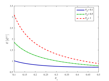
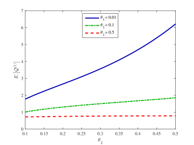
Figure 3: $E\left[\mathcal{Q}^{\left(1\right)}\right]$ vs $\theta_{1}$ and $\theta_{2}$

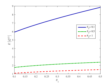
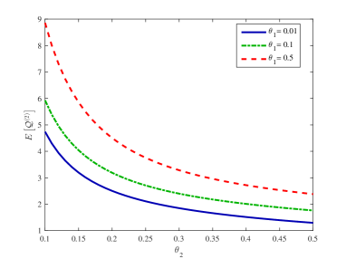
Figure 4: $E\left[\mathcal{Q}^{\left(2\right)}\right]$ vs $\theta_{1}$ and $\theta_{2}$

The two numerical results are intuitive. As $\theta_{1}$ increases, more and more A-customers quickly leave the system so that $E\left[\mathcal{Q}^{\left(1\right)}\right]$ decreases. On the other hand, as $\theta_{2}$ increases, more and more B-customers quickly leave the system so that the probability that an A-customer can match a B-customer will become smaller and smaller. Thus, $E\left[\mathcal{Q}^{\left(1\right)}\right]$ increases as $\theta_{2}$ increases.

5 The Sojourn Time

In this section, we compute the average sojourn time of any arriving A- or B-customer in the matched queue with matching batch pair $(m,n)$. Our analysis includes three different parts: Using the Little’s formula, a probabilistic calculation, and an upper bound. Based on this, we can further find some useful random relations in this matched queue.

Part one: Using the Little’s formula

When the matched queue is stable, we denote by $W$ the sojourn time of any arriving A-customer. By using the Little’s formula and the average stationary queue length $E\left[\mathcal{Q}^{\left(1\right)}\right]$ of the A-customers, we obtain

$$E\left[W\right]=\frac{E\left[\mathcal{Q}^{\left(1\right)}\right]}{\lambda_{1}}.$$ (15)

Part two: A probabilistic calculation

Although the Little’s formula provides a simple method to compute the average sojourn time $E\left[W\right]$, it is still necessary and useful for discussing the random structure of $E\left[W\right]$. To this end, our analysis contains three different cases as follows:

(a) An arriving A-customer observes the system state $\left(i,j\right)$ for $0\leq i\leq m-1$ and $j\geq n$;

(b) an arriving A-customer observes the system state $\left(i,j\right)$ for $0\leq i\leq m-1$ and $0\leq j\leq n-1$; and

(c) an arriving A-customer observes the system state $\left(i,j\right)$ for $i\geq m$ and $0\leq j\leq n-1$.

The following lemma is useful for our computation in the above three cases, while its proof is easy and is omitted here.

Lemma 1.

Let $C$ and $D$ be two independent nonnegative random variables. Then

$$E\left[\min\left\{C,D\right\}\right]=\int_{0}^{+\infty}P\left\{\min\left\{C,D\right\}>x\right\}\text{d}x=\int_{0}^{+\infty}P\left\{C>x\right\}P\left\{C>x\right\}\text{d}x.$$

Now, we use Lemma 1 to compute the average sojourn time $E\left[W\right]$ from three different cases.

Case a: An arriving A-customer observes the system state $\left(i,j\right)$ for $0\leq i\leq m-1$ and $j\geq n$

In this case, if $i=m-1$, then the arriving A-customer makes the number of A-customers become $m$. In this case, the $m$ A-customers can match $n$ B-customers as a group, the $m+n$ customers leave this system immediately. Thus the average sojourn time is given by

$$E\left[W\right]=0.$$ (16)

If $0\leq i\leq m-2$, then the arriving A-customer still needs to wait for $m-\left(i+1\right)$ arrivals of A-customers such that the number of A-customers is $m$. Thus the $m$ A-customers can match $n$ B-customers as a group, which leaves this system immediately.

Let $X_{k}$ be the $k$th interarrival time of the Poisson process with arrival rate $\lambda_{1}$, and $Z$ be the exponential impatient time of A-customer with impatient rate $\theta_{1}$. Then

$$W=\min\left\{Z,\sum_{k=1}^{m-\left(i+1\right)}X_{k}\right\}.$$

This gives

$$E\left[W\right]=\int_{0}^{+\infty}P\left\{Z>x\right\}P\left\{\sum_{k=1}^{m-\left(i+1\right)}X_{k}>x\right\}\text{d}x.$$

Note that $\sum_{k=1}^{m-\left(i+1\right)}X_{k}$ is an Erlang-$\left(m-i-1\right)$ distribution, we have

$$P\left\{\sum_{k=1}^{m-\left(i+1\right)}X_{k}>u\right\}=e^{-\lambda_{1}u}\sum_{k=0}^{m-\left(i+1\right)-1}\frac{\left(\lambda_{1}u\right)^{k}}{k!},$$

this gives

$$E\left[W\right]=\int_{0}^{+\infty}e^{-\left(\lambda_{1}+\theta_{1}\right)x}\sum_{k=0}^{m-\left(i+1\right)-1}\frac{\left(\lambda_{1}x\right)^{k}}{k!}\text{d}x.$$ (17)

Case b: An arriving A-customer observes the system state $\left(i,j\right)$ for $0\leq i\leq m-1$ and $0\leq j\leq n-1$

In this case, if $i=m-1$, then the arriving A-customer makes that the number of A-customers become $m$. However, they still need to wait for $n-j$ arrivals of B-customers such that the number of B-customers is $n$. In this case, the $n$ B-customers can match $m$ A-customers as a group, which leaves this system immediately.

Let $Y_{k}$ be the $k$th interarrival time of the Poisson process with arrival rate $\lambda_{2}$. Then

$$W=\min\left\{Z,\sum_{k=1}^{n-j}Y_{k}\right\}.$$

This gives

$$E\left[W\right] =\int_{0}^{+\infty}P\left\{Z>x\right\}P\left\{\sum_{k=1}^{n-j}Y_{k}>x\right\}\text{d}x$$

$$=\int_{0}^{+\infty}e^{-\left(\lambda_{2}+\theta_{1}\right)x}\sum_{k=0}^{n-j-1}\frac{\left(\lambda_{2}x\right)^{k}}{k!}\text{d}x.$$ (18)

If $0\leq i\leq m-2$, then we still need to not only wait for $m-\left(i+1\right)$ arrivals of A-customers such that the number of A-customers is $m$, but also wait for $n-j$ arrivals of B-customers such that the number of B-customers is $n$. In this case, the $n$ B-customers can match $m$ A-customers as a group, which leaves this system immediately. Thus we obtain

$$W=\min\left\{Z,\max\left\{\sum_{k=1}^{m-\left(i+1\right)}X_{k},\sum_{k=1}^{n-j}Y_{k}\right\}\right\}.$$

This gives

$$E\left[W\right] =\int_{0}^{+\infty}P\left\{Z>x\right\}P\left\{\max\left\{\sum_{k=1}^{m-\left(i+1\right)}X_{k},\sum_{k=1}^{n-j}Y_{k}\right\}>x\right\}\text{d}x$$

$$=\int_{0}^{+\infty}P\left\{Z>x\right\}\left[1-P\left\{\max\left\{\sum_{k=1}^{m-\left(i+1\right)}X_{k},\sum_{k=1}^{n-j}Y_{k}\right\}\leq x\right\}\right]\text{d}x$$

$$=\int_{0}^{+\infty}P\left\{Z>x\right\}\left[1-P\left\{\sum_{k=1}^{m-\left(i+1\right)}X_{k}\leq x\right\}P\left\{\sum_{k=1}^{n-j}Y_{k}\leq x\right\}\right]\text{d}x.$$ (19)

Case c: An arriving A-customer observes the system state $\left(i,j\right)$ for $i\geq m$ and $0\leq j\leq n-1$.

Since $i\geq m$, there exists a unique positive integer $h$ such that $i=hm+f$, where $0\leq f\leq m-1$.

If $f=m-1$, then the arriving A-customer makes the number of A-customers become $\left(h+1\right)m$. We still need to wait for $hn+n-j$ arrivals of B-customers such that the number of B-customers becomes $\left(h+1\right)n$. In this case, the $\left(h+1\right)n$ B-customers can match $\left(h+1\right)m$ A-customers as $h+1$ groups, $\left(h+1\right)\left(m+n\right)$ customers leave this system immediately. Thus we obtain

$$W=\min\left\{Z,\sum_{k=1}^{hn+n-j}Y_{k}\right\}.$$

This gives

$$E\left[W\right] =\int_{0}^{+\infty}P\left\{Z>x\right\}P\left\{\sum_{k=1}^{hn+n-j}Y_{k}>x\right\}\text{d}x$$

$$=\int_{0}^{+\infty}e^{-\left(\lambda_{2}+\theta_{1}\right)x}\sum_{k=0}^{hn+n-j-1}\frac{\left(\lambda_{2}x\right)^{k}}{k!}\text{d}x.$$ (20)

If $0\leq f\leq m-2$, then we still need to not only wait for $m-\left(f+1\right)$ arrivals of A-customers such that the number of A-customers becomes $\left(h+1\right)m$, but also wait for $hn+n-j$ arrivals of B-customers such that the number of B-customers becomes $\left(h+1\right)n$. In this case, the $\left(h+1\right)n$ B-customers can match $\left(h+1\right)m$ A-customers to form $h+1$ groups, which leave this system immediately. Thus we obtain

$$W=\min\left\{Z,\max\left\{\sum_{k=1}^{m-f-1}X_{k},\sum_{k=1}^{hn+n-j}Y_{k}\right\}\right\}.$$

This gives

$$E\left[W\right] =\int_{0}^{+\infty}P\left\{Z>x\right\}P\left\{\max\left\{\sum_{k=1}^{m-f-1}X_{k},\sum_{k=1}^{hn+n-j}Y_{k}\right\}>x\right\}\text{d}x$$

$$=\int_{0}^{+\infty}P\left\{Z>x\right\}\left[1-P\left\{\sum_{k=1}^{m-f-1}X_{k}\leq x\right\}P\left\{\sum_{k=1}^{hn+n-j}Y_{k}\leq x\right\}\right]\text{d}x.$$ (21)

In what follows we provide an average stationary sojourn time of any arriving A-customer by means of Equations (16) to (21) as well as the stationary probability vector of this system. We write that for $l=-1,-2,-3,...$,

$$\Phi_{l} =\left(\phi_{m-1,\left(-l\right)n+n-1},\phi_{m-2,\left(-l\right)n+n-1},\ldots,\phi_{0,\left(-l\right)n+n-1};\ldots;\right.$$

$$\text{ \ \ \ }\left.\phi_{m-1,\left(-l\right)n},\phi_{m-2,\left(-l\right)n},\ldots,\phi_{0,\left(-l\right)n}\right),$$

for $k=0$,

$$\Phi_{0}=\left(\phi_{1,0},\phi_{1,1},\ldots,\phi_{1,n-1};\phi_{2,0},\phi_{2,1},\ldots,\phi_{2,n-1};\ldots;\phi_{m-1,0},\phi_{m-1,1},\ldots,\phi_{m-1,n-1}\right),$$

for $k=1,2,3,...$,

$$\Phi_{k} =\left(\phi_{km,0},\phi_{km,1},\ldots,\phi_{km,n-1};\phi_{km+1,0},\phi_{km+1,1},\ldots,\phi_{km+1,n-1};\ldots;\right.$$

$$\text{ \ \ \ }\left.\phi_{km+m-1,0},\phi_{km+m-1,1},\ldots,\phi_{km+m-1,n-1}\right),$$

and

$$\Phi=\left(\ldots,\Phi_{-2},\Phi_{-1},\Phi_{0},\Phi\pi_{1},\Phi_{2},\ldots\right).$$ (22)

For $1\leq i\leq m-1$ and $0\leq j\leq n-1$; $1\leq i\leq m-1$ and $j\geq n$; and $i\geq m$ and $0\leq j\leq n-1$, we write

$$\phi_{i,j}=\frac{1}{1-\sum\limits_{-\infty<l\leq 0}\sum\limits_{j=0}^{n-1}\phi_{0,\left(-l\right)n+j}}\pi_{i,j}.$$

It is clear that $\Phi e=1$.

When the matched queue with matching batch pair $(m,n)$ is stable, we assume that an arriving A-customer enters State $\left(i-1,j\right)$ with probability $\phi_{i,j}$ for $i\geq 1$ at time $0$. Once the A-customer enters the matched queue, the number of A-customers becomes $i$. In this case, we obtain

$$E\left[W\right]= \sum_{i=1}^{m-1}\sum_{j=n}^{\infty}\phi_{i,j}E\left[W\text{ }|\text{ }\left(N_{1}\left(0\right),N_{2}\left(0\right)\right)=\left(i,j\right)\right]\text{ \ \ \ \ \ \ \ \ \ \ \ Case a}$$

$$+\sum_{i=1}^{m-1}\sum_{j=0}^{n-1}\phi_{i,j}E\left[W\text{ }|\text{ }\left(N_{1}\left(0\right),N_{2}\left(0\right)\right)=\left(i,j\right)\right]\text{ \ \ \ \ \ \ \ \ Case b}$$

$$+\sum_{i=m}^{\infty}\sum_{j=1}^{n-1}\phi_{i,j}E\left[W\text{ }|\text{ }\left(N_{1}\left(0\right),N_{2}\left(0\right)\right)=\left(i,j\right)\right],\text{\ \ \ \ \ \ \ \ Case c}$$ (23)

where $E\left[W\text{ }|\text{ }\left(N_{1}\left(0\right),N_{2}\left(0\right)\right)=\left(i,j\right)\right]$ is given in Case a by (16) and (17); Case b by (18) and (19); and Case c by (20) and (21).

Part three: An upper bound

Now, we provide a better upper bound of the average sojourn time $E\left[W\right]$ given in (23) by means of a new PH distribution of bidirectional infinite sizes.

We write a first passage time of the Markov process $Q$ (or $\left\{\left(N_{1}\left(t\right),N_{2}\left(t\right)\right),\text{ }t\geq 0\right\}$) as

$$\xi=\inf\left\{t:N_{1}\left(t\right)=0\right\},$$

that is, $\xi$ is such a first passage time that the the waiting room of A-customers becomes empty for the first time. It is easy to see that $E\left[W\right]\leq E\left[\xi\right]$, since it is possible that the waiting room of A-customers still contains some customers at the time that the arriving A-customer leaves the system. Note that the arriving A-customer enters State $\left(i-1,j\right)$ with probability $\phi_{i,j}$ for $i\geq 1$ at time $0$. It is also possible that the waiting room of A-customers is empty at the time that the arriving A-customer leaves the system. Thus $E\left[\xi\right]$ can be a better upper bound of the average sojourn time $E\left[W\right]$.

Now, we compute the average first passage time $E\left[\xi\right]$. To do this, we take all the states: $\left(0,k\right)$ for $k\geq 0$, as an absorbing state $\Delta$. Therefore, from the Markov process $Q$, we can set up an absorbing Markov process whose infinitesmall generator is given by

$$\mathbb{Q}=\left(\begin{array}[c]{cc}0&\mathbf{0}\\ T^{0}&T\end{array}\right),$$

where the first row and the first column of the matrix $\mathbb{Q}$ are related to the absorbing state $\Delta$. To write the matrix $T$, we need to check the levels of the absorbing Markov process $\mathbb{Q}$ as follows: For $k\geq 1,$

$$\widetilde{\text{Level }k}=\text{Level }k,$$

$$\widetilde{\text{Level }0}= \left\{\left(1,0\right),\text{ }\left(1,1\right),,\ldots,\text{\ }\left(1,n-1\right);\left(2,0\right),\left(2,1\right),\ldots,\left(2,n-1\right);\right.$$

$$\left.\ldots;\text{\ }\left(m-1,0\right),\text{\ }\left(m-1,1\right),\ldots,\text{\ }\left(m-1,n-1\right)\right\},$$

and $l\leq-1,$

$$\widetilde{\text{Level }l}= \left\{\left(m-1,\left(-l\right)n+n-1\right),\left(m-2,\left(-l\right)n+n-1\right),\ldots,\left(1,\left(-l\right)n+n-1\right);\ldots;\right.$$

$$\left(m-1,\left(-l\right)n+1\right),\left(m-2,\left(-l\right)n+1\right),\ldots,\left(1,\left(-l\right)n+1\right);$$

$$\left.\left(m-1,\left(-l\right)n\right),\left(m-2,\left(-l\right)n\right),\ldots,\left(1,\left(-l\right)n\right)\right\},$$

Thus the state space of the absorbing Markov process $\mathbb{Q}$ is given by

$$\widetilde{\Omega} =\left\{\Delta\right\}\cup\left\{\bigcup\limits_{-\infty<k<\infty}\widetilde{\text{Level }k}\right\}$$

$$=\left\{\Delta\right\}\cup\left\{\bigcup\limits_{k=1}^{\infty}\text{Level }k\right\}\cup\left\{\bigcup\limits_{-\infty<l\leq 0}\widetilde{\text{Level }l}\right\}.$$

By using the levels: Level $k$ for $k\geq 1$ and $\widetilde{\text{Level }l}$ for $-\infty<l\leq 0$, we obtain

$$T=\left(\begin{array}[c]{ccccccccccc}\ddots&\ddots&\ddots&&&&&&&&\\ &\widetilde{B}_{0}^{\left(-3\right)}&\widetilde{B}_{1}^{\left(-3\right)}&\widetilde{B}_{2}^{\left(-3\right)}&&&&&&&\\ &&\widetilde{B}_{0}^{\left(-2\right)}&\widetilde{B}_{1}^{\left(-2\right)}&\widetilde{B}_{2}^{\left(-2\right)}&&&&&&\\ &&&\widetilde{B}_{0}^{\left(-1\right)}&\widetilde{B}_{1}^{\left(-1\right)}&\framebox{$\widetilde{B}_{2}^{\left(-1\right)}$}&&&&&\\ &&&&\framebox{$\widetilde{B}_{0}^{\left(0\right)}$}&\framebox{$\widetilde{C}$}&\framebox{$\widetilde{A}_{0}^{\left(0\right)}$}&&&&\\ &&&&&\framebox{$\widetilde{A}_{2}^{\left(1\right)}$}&A_{1}^{\left(1\right)}&A_{0}^{\left(1\right)}&&&\\ &&&&&&A_{2}^{\left(2\right)}&A_{1}^{\left(2\right)}&A_{0}^{\left(2\right)}&&\\ &&&&&&&A_{2}^{\left(3\right)}&A_{1}^{\left(3\right)}&A_{0}^{\left(3\right)}&\\ &&&&&&&&\ddots&\ddots&\ddots\end{array}\right),$$

where $\widetilde{A}_{0}^{\left(0\right)}$, $\widetilde{C}$, $\widetilde{A}_{2}^{\left(1\right)}$, $\widetilde{B}_{0}^{\left(0\right)}$ and $\widetilde{B}_{i}^{\left(-l\right)}$ for $i=0,1,2$ and $l\leq-1$, can be written easily and their details are omitted here.

The following theorem shows that the first passage time $\xi$ is of bidirectional infinite phase type, and thus provides a method to compute the average first passage time $E\left[\xi\right]$. The proof is easy and is omitted here.

Theorem 3.

If the arriving A-customer enters State $\left(i-1,j\right)$ with probability $\phi_{i,j}$ for $i\geq 1$ at time $0$, then the first passage time $\xi$ is of bidirectional infinite phase type with an irreducible representation $\left(\Phi,T\right)$, and

$$E\left[\xi\right]=-\Phi T^{-1}e\text{,}$$ (24)

where $\Phi$ is given in (22), $T^{-1}$ is the maximal non-positive inverse of the matrix $T$.

When the PH distribution is unilateral infinite, Chapter 8 of Li [48] provides a detailed discussion for how to compute the maximal non-positive inverse matrix $T^{-1}$ of infinite sizes by means of the RG-factorizations given in Li [48]. Furthermore, if $T$ is the infinitesmall generator of an irreducible QBD process, then the maximal non-positive inverse matrix $T^{-1}$ can be explicitly expressed by means of the $R$-, $U$- and $G$-measures.

When the PH distribution is bidirectional infinite, to our best knowledge, this paper is the first to deal with the maximal non-positive inverse matrix $T^{-1}$ of bidirectional infinite sizes. To this end, we write

$$T=\left(\begin{array}[c]{cc}T_{1,1}&T_{1,2}\\ T_{2,1}&T_{2,2}\end{array}\right),$$

where

$$T_{1,1}=\left(\begin{array}[c]{ccccc}\ddots&\ddots&\ddots&&\\ &\widetilde{B}_{0}^{\left(-2\right)}&\widetilde{B}_{1}^{\left(-2\right)}&\widetilde{B}_{2}^{\left(-2\right)}&\\ &&\widetilde{B}_{0}^{\left(-1\right)}&\widetilde{B}_{1}^{\left(-1\right)}&\widetilde{B}_{2}^{\left(-1\right)}\\ &&&\widetilde{B}_{0}^{\left(0\right)}&\widetilde{C}\end{array}\right),\text{ }T_{1,2}=\left(\begin{array}[c]{ccccc}&&&&\\ &&&&\\ &&&&\\ \widetilde{A}_{0}^{\left(0\right)}&&&&\end{array}\right),$$

$$T_{2,1}=\left(\begin{array}[c]{ccccc}&&&&\widetilde{A}_{2}^{\left(1\right)}\\ &&&&\\ &&&&\\ &&&&\end{array}\right),\text{ }T_{2,2}=\left(\begin{array}[c]{ccccc}A_{1}^{\left(1\right)}&A_{0}^{\left(1\right)}&&&\\ A_{2}^{\left(2\right)}&A_{1}^{\left(2\right)}&A_{0}^{\left(2\right)}&&\\ &A_{2}^{\left(3\right)}&A_{1}^{\left(3\right)}&A_{0}^{\left(3\right)}&\\ &&\ddots&\ddots&\ddots\end{array}\right).$$

Note that the Markov chain $Q$ is irreducible and $T_{2,1}e\gneq 0$ due to $\widetilde{A}_{2}^{\left(1\right)}e\gneq 0$, thus the submatrix $T_{2,2}$ must be invertible. Based on this, it is easy to check that

$$T^{-1}=\left[\begin{array}[c]{c}T_{1,1;2}^{-1}\text{ \ \ \ \ \ \ \ \ \ }-T_{1,1;2}^{-1}T_{1,2}T_{2,2}^{-1}\\ -T_{2,2}^{-1}T_{2,1}T_{1,1;2}^{-1}\text{ \ \ \ \ }T_{2,2}^{-1}+T_{2,2}^{-1}T_{2,1}T_{1,1;2}^{-1}T_{1,2}T_{2,2}^{-1}\end{array}\right],$$ (25)

where

$$T_{1,1;2}=T_{1,1}-T_{1,2}T_{2,2}^{-1}T_{2,1}.$$ (26)

It is easy to see that the maximal non-positive inverse matrix $T^{-1}$ of bidirectional infinite sizes can be expressed by means of the maximal non-positive inverse matrix $T_{2,2}^{-1}$ of unilateral infinite sizes. This relation plays a key role in setting up the PH distribution of bidirectional infinite sizes.

In what follows, we simply discuss the maximal non-positive inverse matrix $T_{2,2}^{-1}$ of unilateral infinite sizes by means of the RG-factorizations, e.g., see Chapter 1 of Li [48] or Li and Cao [50] for more details.

For the QBD process $T_{2,2}$ of unilateral infinite sizes, we define the UL-type $\mathbf{U}$-, $\mathbf{R}$- and $\mathbf{G}$-measures as

$$\mathbf{U}_{k}=A_{1}^{\left(k\right)}+A_{0}^{\left(k\right)}\left(-\mathbf{U}_{k+1}^{-1}\right)A_{2}^{\left(k+1\right)},\text{ \ }k\geq 1,$$

$$\mathbf{R}_{k}=A_{0}^{\left(k\right)}\left(-\mathbf{U}_{k+1}^{-1}\right),\text{ \ }k\geq 1,$$

and

$$\mathbf{G}_{k}=\left(-\mathbf{U}_{k}^{-1}\right)A_{2}^{\left(k\right)},\text{ \ }k\geq 2.$$

Note that the matrix sequence $\left\{\mathbf{R}_{k},k\geq 1\right\}$ is the minimal nonnegative solution to the system of nonlinear matrix equations

$$A_{0}^{\left(k\right)}+\mathbf{R}_{k}A_{1}^{\left(k+1\right)}+\mathbf{R}_{k}\mathbf{R}_{k+1}A_{2}^{\left(k+2\right)}=0,\text{ \ }k\geq 1;$$

and the matrix sequence $\left\{\mathbf{G}_{k},k\geq 2\right\}$ is the minimal nonnegative solution to the system of nonlinear matrix equations

$$A_{0}^{\left(k\right)}\mathbf{G}_{k+1}\mathbf{G}_{k}+A_{1}^{\left(k\right)}\mathbf{G}_{k}+A_{2}^{\left(k\right)}=0,\text{ \ }k\geq 2.$$

Based on this, the UL-type RG-factorization of the matrix $T_{2,2}$ of unilateral infinite sizes is given by

$$T_{2,2}=\left(I-\mathbf{R}_{U}\right)\mathbf{U}_{D}\left(I-\mathbf{G}_{L}\right),$$ (27)

where

$$I-\mathbf{R}_{U}=\left(\begin{array}[c]{ccccc}I&-\mathbf{R}_{1}&&&\\ &I&-\mathbf{R}_{2}&&\\ &&I&-\mathbf{R}_{3}&\\ &&&I&\ddots\\ &&&&\ddots\end{array}\right),$$

$$\mathbf{U}_{D}=\text{diag}\left(\mathbf{U}_{1},\mathbf{U}_{2},\mathbf{U}_{3},\ldots\right),$$

$$I-\mathbf{G}_{L}=\left(\begin{array}[c]{ccccc}I&&&&\\ -\mathbf{G}_{2}&I&&&\\ &-\mathbf{G}_{3}&I&&\\ &&-\mathbf{G}_{4}&I&\\ &&&\ddots&\ddots\end{array}\right).$$

By using $\mathbf{R}$-measure $\left\{\mathbf{R}_{k}:k\geq 1\right\}$ and the $\mathbf{G}$-measure $\left\{\mathbf{G}_{k}:k\geq 2\right\}$, we write

$$X_{k}^{\left(k\right)}=I,$$

$$X_{k+l}^{\left(k\right)}=\mathbf{R}_{k}\mathbf{R}_{k+1}\cdots\mathbf{R}_{k+l-1},\text{ }k\geq 1,\text{ }l\geq 1,$$

$$Y_{k}^{\left(k\right)}=I,$$

$$Y_{k-l}^{\left(k\right)}=\mathbf{G}_{k}\mathbf{G}_{k-1}\cdots\mathbf{G}_{k-l+1},\text{ }k>l\geq 1.$$

From the UL-type RG-factorization (27), it is easy to check that the three matrices $I-\mathbf{R}_{U}$, $\mathbf{U}_{D}$ and $I-\mathbf{G}_{L}$ are all invertible, and

$$\left(I-\mathbf{R}_{U}\right)^{-1}=\left(\begin{array}[c]{ccccc}X_{1}^{\left(1\right)}&X_{2}^{\left(1\right)}&X_{3}^{\left(1\right)}&X_{4}^{\left(1\right)}&\ldots\\ &X_{2}^{\left(2\right)}&X_{3}^{\left(2\right)}&X_{4}^{\left(2\right)}&\ldots\\ &&X_{3}^{\left(3\right)}&X_{4}^{\left(3\right)}&\ldots\\ &&&X_{4}^{\left(4\right)}&\ldots\\ &&&&\ddots\end{array}\right),$$

$$\mathbf{U}_{D}^{-1}=\text{diag}\left(\mathbf{U}_{1}^{-1},\mathbf{U}_{2}^{-1},\mathbf{U}_{3}^{-1},\mathbf{U}_{4}^{-1},\ldots\right),$$

$$\left(I-\mathbf{G}_{L}\right)^{-1}=\left(\begin{array}[c]{ccccc}Y_{1}^{\left(1\right)}&&&&\\ Y_{1}^{\left(2\right)}&Y_{2}^{\left(2\right)}&&&\\ Y_{1}^{\left(3\right)}&Y_{2}^{\left(3\right)}&Y_{3}^{\left(3\right)}&&\\ Y_{1}^{\left(4\right)}&Y_{2}^{\left(4\right)}&Y_{3}^{\left(4\right)}&Y_{4}^{\left(4\right)}&\\ \vdots&\vdots&\vdots&\vdots&\ddots\end{array}\right).$$

We obtain

$$T_{2,2}^{-1}=\left(I-\mathbf{G}_{L}\right)^{-1}\mathbf{U}_{D}^{-1}\left(I-\mathbf{R}_{U}\right)^{-1}.$$ (28)

By using (25), (26) and (28), we obtain the maximal non-positive inverse matrix $T^{-1}$ of bidirectional infinite sizes. Therefore, we can compute the average first passage time $E\left[\xi\right]$, and $E\left[W\right]\leq E\left[\xi\right]$.

6 The Departure Process

In this section, we use the MMAP of bidirectional infinite sizes to discuss the departure process with three types of customers (i.e., impatient A-customers, impatient B-customers, and groups of $m$ A-customers and $n$ B-customers) in the matched queue with matching batch pair $(m,n)$.

To set up the MMAP of bidirectional infinite sizes, we need to establish four matrices: $D_{0}$, $D_{A}$, $D_{B}$ and $D_{AB}$, where $D_{A}$ and $D_{B}$ are the departure-rate matrices of A-customers and B-customers due to their impatient behavior, respectively; $D_{AB}$ is the departure-rate matrix of groups matched by $m$ A-customers and $n$ B-customers; and $D_{0}$ is the transition rate matrix of stochastic environment in the MMAP. From the infinitesimal generator (4), we have

$$D_{0}=Q-D_{A}-D_{B}-D_{AB},$$ (29)

where

$$D_{A}=\left(\begin{array}[c]{ccccccc}\ddots&&&&&&\\ \ddots&D_{A}^{\left(-2\right)}&&&&&\\ &0&D_{A}^{\left(-1\right)}&&&&\\ &&0&D_{A}^{\left(0\right)}&&&\\ &&&\widetilde{D}_{A}^{\left(1\right)}&D_{A}^{\left(1\right)}&&\\ &&&&\widetilde{D}_{A}^{\left(2\right)}&D_{A}^{\left(2\right)}&\\ &&&&&\ddots&\ddots\end{array}\right),$$ (30)

$$D_{A}^{\left(k\right)}=\left(\begin{array}[c]{ccccc}0&&&&\\ A_{1,1}^{\left(k\right)}&0&&&\\ &\ddots&\ddots&&\\ &&A_{1,m-2}^{\left(k\right)}&0&\\ &&&A_{1,m-1}^{\left(k\right)}&0\end{array}\right)_{mn\times mn},k\geq 0,$$

$$A_{1,i}^{\left(k\right)}=\left(\begin{array}[c]{cccc}\left(km+i\right)\theta_{1}&&&\\ &\left(km+i\right)\theta_{1}&&\\ &&\ddots&\\ &&&\left(km+i\right)\theta_{1}\end{array}\right)_{n\times n},1\leq i\leq m-1,$$

$$D_{A}^{\left(l\right)}=\left(\begin{array}[c]{ccccc}A_{1,1}&&&&\\ &A_{1,2}&&&\\ &&\ddots&&\\ &&&A_{1,n-1}&\\ &&&&A_{1,n}\end{array}\right)_{nm\times nm},\text{ }l\leq-1,$$

$$A_{1,i}=\left(\begin{array}[c]{ccccc}0&\left(m-1\right)\theta_{1}&&&\\ &0&\left(m-2\right)\theta_{1}&&\\ &&0&\ddots&\\ &&&\ddots&\theta_{1}\\ &&&&0\end{array}\right)_{m\times m},\text{ }1\leq i\leq n,$$

$$\widetilde{D}_{A}^{\left(k\right)}=\left(\begin{array}[c]{cc}{\Large 0}_{n\times\left[\left(m-1\right)n\right]}&\left.\begin{array}[c]{ccc}km\theta_{1}&&\\ &\ddots&\\ &&km\theta_{1}\end{array}\right\}n\times n\\ &{\Large 0}_{\left[\left(m-1\right)n\right]\times n}\text{ }\end{array}\right)_{mn\times mn},\text{\ }k\geq 1;$$

$$D_{B}=\left(\begin{array}[c]{ccccccc}\ddots&\ddots&&&&&\\ &D_{B}^{\left(-2\right)}&\widetilde{D}_{B}^{\left(-2\right)}&&&&\\ &&D_{B}^{\left(-1\right)}&\widetilde{D}_{B}^{\left(-1\right)}&&&\\ &&&D_{B}^{\left(0\right)}&0&&\\ &&&&D_{B}^{\left(1\right)}&0&\\ &&&&&D_{B}^{\left(2\right)}&\ddots\\ &&&&&&\ddots\end{array}\right),$$ (31)

$$D_{B}^{\left(k\right)}=\left(\begin{array}[c]{ccccc}B_{1,1}&&&&\\ &B_{1,2}&&&\\ &&\ddots&&\\ &&&B_{1,m-1}&\\ &&&&B_{1,m}\end{array}\right)_{mn\times mn},k\geq 0,$$

$$B_{1,i}=\left(\begin{array}[c]{ccccc}0&&&&\\ \theta_{2}&\ddots&&&\\ &\ddots&0&&\\ &&\left(n-2\right)\theta_{2}&0&\\ &&&\left(n-1\right)\theta_{2}&0\end{array}\right)_{n\times n},\text{ }1\leq i\leq m,$$

$$D_{B}^{\left(l\right)}=\left(\begin{array}[c]{ccccc}0&B_{1,1}^{\left(l\right)}&&&\\ &0&B_{1,2}^{\left(l\right)}&&\\ &&\ddots&\ddots&\\ &&&0&B_{1,n-1}^{\left(l\right)}\\ &&&&0\end{array}\right)_{nm\times nm},\text{ }l\leq-1,$$

$$B_{1,i}^{\left(l\right)}=\left(\begin{array}[c]{cccc}\left(-ln+n-i\right)\theta_{2}&&&\\ &\left(-ln+n-i\right)\theta_{2}&&\\ &&\ddots&\\ &&&\left(-ln+n-i\right)\theta_{2}\end{array}\right)_{m\times m},1\leq i\leq n-1,$$

$$\widetilde{D}_{B}^{\left(-1\right)}=\left(\begin{array}[c]{cccc}{\Large 0}_{\left[\left(n-1\right)m\right]\times n}&{\Large 0}_{\left[\left(n-1\right)m\right]\times n}&\cdots&{\Large 0}_{\left[\left(n-1\right)m\right]\times n}\\ \text{\ }\left.\begin{array}[c]{cc}0&0\\ \vdots&\vdots\\ 0&0\\ 0&n\theta_{2}\end{array}\right\}m\times n&\text{\ }\left.\begin{array}[c]{cc}0&0\\ \vdots&\vdots\\ 0&n\theta_{2}\\ 0&0\end{array}\right\}m\times n&\cdots&\text{ \ }\left.\begin{array}[c]{cc}0&n\theta_{2}\\ \vdots&\vdots\\ 0&0\\ 0&0\end{array}\right\}m\times n\end{array}\right)_{mn\times mn},$$

$$\widetilde{D}_{B}^{\left(l\right)}=\left(\begin{array}[c]{cc}{\Large 0}_{\left[\left(n-1\right)m\right]\times m}\text{\ \ \ \ \ \ }&{\Large 0}_{\left[\left(n-1\right)m\right]\times\left[\left(n-1\right)m\right]}\\ \left.\begin{array}[c]{ccc}-ln\theta_{2}&&\\ &\ddots&\\ &&-ln\theta_{2}\end{array}\right\}m\times m&{\Large 0}_{m\times\left[\left(n-1\right)m\right]}\end{array}\right)_{mn\times mn},\text{ }l\leq-2;$$

$$D_{AB}=\left(\begin{array}[c]{ccccccccc}\ddots&\ddots&&&&&&&\\ \ddots&0&D_{AB}^{\left(-3\right)}&&&&&&\\ &0&0&D_{AB}^{\left(-2\right)}&&&&&\\ &&0&0&D_{AB}^{\left(-1\right)}&&&&\\ &&&0&0&0&&&\\ &&&&D_{AB}^{\left(1\right)}&0&0&&\\ &&&&&D_{AB}^{\left(2\right)}&0&0&\\ &&&&&&D_{AB}^{\left(3\right)}&0&\ddots\\ &&&&&&&\ddots&\ddots\end{array}\right),$$ (32)

$$D_{AB}^{\left(k\right)}=\left(\begin{array}[c]{ccc}\left.\begin{array}[c]{ccc}0&&\\ &\ddots&\\ \lambda_{2}&&0\end{array}\right\}n\times n&&\\ &\ddots&\\ &&\left.\begin{array}[c]{ccc}0&&\\ &\ddots&\\ \lambda_{2}&&0\end{array}\right\}n\times n\end{array}\right)_{mn\times mn},\text{\ }k\geq 1,$$

$$D_{AB}^{\left(-1\right)}=\left(\begin{array}[c]{cc}\left.\begin{array}[c]{cccc}0&\cdots&0&\lambda_{1}\\ \vdots&&\vdots&\vdots\\ 0&\cdots&0&0\end{array}\right\}m\times n&{\Large 0}_{m\times\left[\left(m-1\right)n\right]}\\ \left.\begin{array}[c]{cccc}0&\cdots&\lambda_{1}&0\\ \vdots&&\vdots&\vdots\\ 0&\cdots&0&0\end{array}\right\}m\times n&{\Large 0}_{m\times\left[\left(m-1\right)n\right]}\\ \vdots\text{\ \ }&\vdots\\ \left.\begin{array}[c]{cccc}\lambda_{1}&\cdots&0&0\\ \vdots&&\vdots&\vdots\\ 0&\cdots&0&0\end{array}\right\}m\times n&{\Large 0}_{m\times\left[\left(m-1\right)n\right]}\end{array}\right)_{mn\times mn},$$

$$D_{AB}^{\left(l\right)}=\left(\begin{array}[c]{ccc}\left.\begin{array}[c]{ccc}0&&\lambda_{1}\\ &\ddots&\\ &&0\end{array}\right\}m\times m&&\\ &\ddots&\\ &&\left.\begin{array}[c]{ccc}0&&\lambda_{1}\\ &\ddots&\\ &&0\end{array}\right\}m\times m\end{array}\right)_{mn\times mn},\text{ }l\leq-2,$$

The following theorem shows that the departure process of the matched queue with matching batch pair $(m,n)$ is an MMAP of bidirectional infinite sizes whose matrix sequence is given by $\left\{D_{0},D_{A},D_{B},D_{AB}\right\}$. The proof is easy and omitted here by means of He and Neuts [32, 33].

Theorem 4.

In the matched queue with matching batch pair $(m,n)$, its departure process has three types of customers: The impatient A- and B-customers, and the groups matched by $m$ A-customers and $n$ B-customers. Also, the departure process with the three types of customers is an MMAP of bidirectional infinite sizes with the matrix sequence $\left\{D_{0},D_{A},D_{B},D_{AB}\right\}$.

Note that the matched queue with matching batch pair $(m,n)$ must be stable. When the stationary probability vector $\pi$ of the Markov process $Q$ is given, we have

(a) the stationary impatient-departure rate of the A-customers is given by

$$\mu_{A}=\pi D_{A}e;$$

(b) the stationary impatient-departure rate of the B-customers is given by

$$\mu_{B}=\pi D_{B}e;$$

(c) the stationary matched-departure rate of the groups matched by $m$ A-customers and $n$ B-customers is given by

$$\mu_{AB}=\pi D_{AB}e.$$

Also, when observing the A- and B-customers, we have

(d) the stationary departure rate of the A-customers is given by

$$\mu_{A}=\pi\left(D_{A}+mD_{AB}\right)e;$$

(e) the stationary departure rate of the B-customers is given by

$$\mu_{A}=\pi\left(D_{B}+nD_{AB}\right)e;$$

(f) the stationary departure rate of the A- and B-customers is given by

$$\mu_{\text{all}}=\pi\left[D_{A}+D_{B}+\left(m+n\right)D_{AB}\right]e.$$

To further understand the departure process with three types of customers, from the infinitesimal generator (4) and the departure-rate matrices (30), (31) and (32), by using (29) we write

$$D_{0}=\left(\begin{array}[c]{ccccccccc}\ddots&\ddots&\ddots&&&&&&\\ &H_{0}^{\left(-2\right)}&H_{1}^{\left(-2\right)}&H_{2}^{\left(-2\right)}&&&&&\\ &&H_{0}^{\left(-1\right)}&H_{1}^{\left(-1\right)}&\framebox{$H_{2}^{\left(-1\right)}$}&&&&\\ &&&\framebox{$H_{0}^{\left(0\right)}$}&F&\framebox{$G_{0}^{\left(0\right)}$}&&&\\ &&&&\framebox{$G_{2}^{\left(1\right)}$}&G_{1}^{\left(1\right)}&G_{0}^{\left(1\right)}&&\\ &&&&&G_{2}^{\left(2\right)}&G_{1}^{\left(2\right)}&G_{0}^{\left(2\right)}&\\ &&&&&&\ddots&\ddots&\ddots\end{array}\right).$$

Note that $D_{0}=Q-D_{A}-D_{B}-D_{AB}$ with $D_{A}+D_{B}+D_{AB}\gneq 0$, and the Markov process $Q$ is irreducible and positive recurrent, thus the Markov process $D_{0}$ is irreducible and transient, so the matrix $D_{0}$ of bidirectional infinite sizes is invertible. To compute the maximal non-positive inverse matrix of $D_{0}$, we write

$$D_{0}=\left(\begin{array}[c]{cc}W_{1,1}&W_{1,2}\\ W_{2,1}&W_{2,2}\end{array}\right),$$

where

$$W_{1,1}=\left(\begin{array}[c]{ccccc}\ddots&\ddots&\ddots&&\\ &H_{0}^{\left(-2\right)}&H_{1}^{\left(-2\right)}&H_{2}^{\left(-2\right)}&\\ &&H_{0}^{\left(-1\right)}&H_{1}^{\left(-1\right)}&H_{2}^{\left(-1\right)}\\ &&&H_{0}^{\left(0\right)}&F\end{array}\right),\text{ }W_{1,2}=\left(\begin{array}[c]{ccccc}&&&&\\ &&&&\\ &&&&\\ G_{0}^{\left(0\right)}&&&&\end{array}\right),$$

$$W_{2,1}=\left(\begin{array}[c]{ccccc}&&&&G_{2}^{\left(1\right)}\\ &&&&\\ &&&&\\ &&&&\end{array}\right),\text{ }W_{2,2}=\left(\begin{array}[c]{ccccc}G_{1}^{\left(1\right)}&G_{0}^{\left(1\right)}&&&\\ G_{2}^{\left(2\right)}&G_{1}^{\left(2\right)}&G_{0}^{\left(2\right)}&&\\ &G_{2}^{\left(3\right)}&G_{1}^{\left(3\right)}&G_{0}^{\left(3\right)}&\\ &&\ddots&\ddots&\ddots\end{array}\right).$$

Since the Markov chain $Q$ is irreducible and $W_{2,1}e\gneq 0$ due to $G_{2}^{\left(1\right)}e\gneq 0$, the submatrix $W_{2,2}$ must be invertible. Based on this, it is easy to check that

$$D_{0}^{-1}=\left(\begin{array}[c]{c}W_{1,1;2}^{-1}\text{ \ \ \ \ \ \ \ \ \ }-W_{1,1;2}^{-1}W_{1,2}W_{2,2}^{-1}\\ -W_{2,2}^{-1}W_{2,1}W_{1,1;2}^{-1}\text{ \ \ \ \ }W_{2,2}^{-1}+W_{2,2}^{-1}W_{2,1}W_{1,1;2}^{-1}W_{1,2}W_{2,2}^{-1}\end{array}\right),$$

where

$$W_{1,1;2}=W_{1,1}-W_{1,2}W_{2,2}^{-1}W_{2,1},$$

and the maximal non-positive inverse matrix $W_{2,2}^{-1}$ of unilateral infinite sizes can be computed by means of the RG-factorizations, as seen in (27).

Let $A$ and $B$ be the impatient departures of the A- and A-customers, respectively; and $AB$ be a departure of the groups matched by $m$ A-customers and $n$ B-customers.

The following theorem describes some probability characteristics of the departure process with the three types of customers, while its proof is easy by using He and Neuts [32], and it is omitted here.

Theorem 5.

In the matched queue with matching batch pair $(m,n)$, its departure process with the three types of customers: The MMAP of bidirectional infinite sizes with the matrix sequence $\left\{D_{0},D_{A},D_{B},D_{AB}\right\}$, has the probability characteristics as follows:

(a) Backward looking: The probability that the last departure before an arbitrary time $t$ is marked by $i\in\left\{A,B,AB\right\}$ is given by $\pi D_{i}\left(-D_{0}^{-1}\right)e$.

(b) Forward looking: The probability that the first departure after an arbitrary time $t$ is marked by $i\in\left\{A,B,AB\right\}$ is given by $\pi\left(-D_{0}^{-1}\right)D_{i}e$.

(c) At the departure: The probability that an arbitrary departure is of type $i$ is given by

$$\frac{\pi D_{i}e}{\pi\left[D_{A}+D_{B}+D_{AB}\right]e},\text{ \ }i\in\left\{A,B,AB\right\}.$$

Finally, we extend the above probability characteristics of the departure process with the three types of customers from a departure point to multiple departure points. We write that $i_{1},i_{2},\ldots,i_{k}\in\left\{A,B,AB\right\}$.

Theorem 6.

(a) Backward looking: Let

$$i_{k}\leftarrow i_{k-1}\leftarrow\cdots\leftarrow i_{2}\leftarrow i_{1}\Longleftarrow t$$

Then the probability that the $k$ consecutive departure points before an arbitrary time $t$ are marked by $i_{1},i_{2},\ldots,i_{k}\in\left\{A,B,AB\right\}$ is given by

$$\pi\left[D_{i_{1}}\left(-D_{0}^{-1}\right)\right]\left[D_{i_{2}}\left(-D_{0}^{-1}\right)\right]\cdots\left[D_{i_{k}}\left(-D_{0}^{-1}\right)\right]e.$$

(b) Forward looking: Let

$$t\Longrightarrow i_{1}\rightarrow i_{2}\rightarrow\cdots\rightarrow i_{k-1}\rightarrow i_{k}$$

Then the probability that the $k$ consecutive departure points after an arbitrary time $t$ are marked by $i_{1},i_{2},\ldots,i_{k}\in\left\{A,B,AB\right\}$ is given by

$$\pi\left[\left(-D_{0}^{-1}\right)D_{i_{1}}\right]\left[\left(-D_{0}^{-1}\right)D_{i_{2}}\right]\cdots\left[\left(-D_{0}^{-1}\right)D_{i_{k}}\right]e.$$

Remark 5.

For the matched queue with matching batch pair $(m,n)$, the analysis of the departure process with the three types of customers is described as the MMAP of bidirectional infinite sizes with the matrix sequence $\left\{D_{0},D_{A},D_{B},D_{AB}\right\}$; while the finite-size case of which was studied in He and Neuts [32]. In the study of MMAPs, we make two useful advances: (1) The maximal non-positive inverse matrix $D_{0}^{-1}$ of bidirectional infinite sizes can be expressed by means of the maximal non-positive inverse matrix $W_{2,2}^{-1}$ of unilateral infinite sizes, and (2) the maximal non-positive inverse matrix $W_{2,2}^{-1}$ of unilateral infinite sizes can be determined by means of the R-, U- and G-measures, as seen in how to compute the maximal non-positive inverse matrix $T^{-1}$ of the previous section. Therefore, our RG-factorization method generalizes the MMAPs of finite sizes given in He and Neuts [32] to the MMAPs of (either unilateral or bidirectional) infinite sizes such that the MMAPs can adapt to a wider range of practical applications.

Remark 6.

It is necessary and useful to study the departure process of the matched queue with matching batch pair $(m,n)$ (and more generally, stochastic models). Such a departure process can be regarded as a new input in a local node of the system. See He et al. [34] for more details. This is very useful in the study of large-scale stochastic networks.

7 Concluding Remarks

In this paper, we discuss an interesting but challenging bilateral stochastically matching problem: A more general matched queue with matching batch pair $(m,n)$ and two types of impatient customers. We show that the matched queue with matching batch pair $(m,n)$ can be expressed as a novel level-dependent QBD process with bidirectional infinite levels. Based on this, we provide a detailed analysis for this matched queue, including the system stability, the average stationary queue lengths, the average sojourn times, and the departure process. We believe that the methodology and results developed in this paper can be applicable to analyze more general matched queues, which are widely encountered in many practical areas, for example, sharing economy, ridesharing platform, bilateral market, organ transplantation, taxi services, assembly systems, and so on.

Along these lines, we will continue our future research on the following directions:

– Considering probabilistic matching system with matching pair $\left(1,1\right)$.

– Studying probabilistic matching system with matching batch pair $\left(m,n\right)$.

– Discussing some Phase-type and MAP factors in the study of matched queues.

– Analyzing fluid and diffusion approximations for matched system with matching batch pair $\left(m,n\right)$.

– Developing stochastic optimization, and Markov decision processes in the study of matched queues.

Appendix

The appendix contains the proofs of Theorems 1 and 2.

Proof of Theorem 1. It is clear that the QBD process $Q$ with bidirectional infinite levels is irreducible through observing Figures 1 and 2, since this matched queue contains two Poisson inputs and two exponential impatient times.

From returning to Level $0$, it is easy to see that the QBD process $Q$ with bidirectional infinite levels is positive recurrent if and only if the two unilateral QBD processes $Q_{A}$ and $Q_{B}$ are both positive recurrent. Thus, our aim is to prove that if $\left(\theta_{1},\theta_{2}\right)>0$, then the two unilateral QBD processes $Q_{A}$ and $Q_{B}$ are both positive recurrent by means of the mean drift technique by Neuts [48] and Li [42].

For the QBD process $Q_{A}$, let $\mathbb{A}_{k}=A_{0}^{\left(k\right)}+A_{1}^{\left(k\right)}+A_{2}^{\left(k\right)}$ in Level $k$. Then

$$\mathbb{A}_{k}=\left(\begin{array}[c]{ccccc}A_{1,1,1}&A_{2,1}&&&A_{2,2,2}\\ A_{3,1}&A_{1,2,1}&A_{2,2}&&\\ &\ddots&\ddots&\ddots&\\ &&A_{3,m-2}&A_{1,m-1,1}&A_{2,m-1}\\ A_{0}&&&A_{3,m-1}&A_{1,m,1}\end{array}\right)_{mn\times mn},$$

where

$$A_{0}=\left(\begin{array}[c]{ccc}\lambda_{1}&&\\ &\ddots&\\ &&\lambda_{1}\end{array}\right)_{n\times n},\text{ }A_{2,2,2}=\left(\begin{array}[c]{ccc}km\theta_{1}&&\\ &\ddots&\\ &&km\theta_{1}\end{array}\right)_{n\times n},$$

$$A_{1,i,1}=\left(\begin{array}[c]{ccccc}a_{1,i}^{\left(1\right)}&\lambda_{2}&&&\\ \theta_{2}&a_{1,i}^{\left(2\right)}&\lambda_{2}&&\\ &\ddots&\ddots&\ddots&\\ &&\left(n-2\right)\theta_{2}&a_{1,i}^{\left(n-1\right)}&\lambda_{2}\\ \lambda_{2}&&&\left(n-1\right)\theta_{2}&a_{1,i}^{\left(n\right)}\end{array}\right)_{n\times n},\text{ }1\leq i\leq m,$$

$$a_{1,i}^{\left(r\right)}=-\left(\lambda_{1}+\lambda_{2}+\left(r-1\right)\theta_{2}+\left(km+i-1\right)\theta_{1}\right),\text{ }1\leq r\leq n,$$

$$A_{2,i}=\left(\begin{array}[c]{cccc}\lambda_{1}&&&\\ &\lambda_{1}&&\\ &&\ddots&\\ &&&\lambda_{1}\end{array}\right)_{n\times n},1\leq i\leq m-1,$$

$$A_{3,i}=\left(\begin{array}[c]{cccc}\left(km+i\right)\theta_{1}&&&\\ &\left(km+i\right)\theta_{1}&&\\ &&\ddots&\\ &&&\left(km+i\right)\theta_{1}\end{array}\right)_{n\times n},1\leq i\leq m-1.$$

Let $\alpha=\left(\alpha_{1},\alpha_{2},...,\alpha_{n};...;\alpha_{\left(m-1\right)n+1},\alpha_{\left(m-1\right)n+2},...,\alpha_{\left(m-1\right)n+n}\right)$ be the stationary probability vector of the Markov process $\mathbb{A}_{k}$. Then

$$\alpha\mathbb{A}_{k}=\mathbf{0},\text{ \ }\alpha\mathbf{e}=1.$$

Note that $\alpha>0$, since the Markov process $\mathbb{A}_{k}$ is irreducible.

Once the stationary probability vector $\alpha$ is obtained, we can compute the (upward and downward) mean drift rates of the QBD process $Q_{A}$. From Level $k$ to Level $k+1$, the upward mean drift rate is given by

$$\alpha A_{0}^{\left(k\right)}\mathbf{e}=\lambda_{1}\left(\alpha_{\left(m-1\right)n+1}+\alpha_{\left(m-1\right)n+2}+\cdots+\alpha_{\left(m-1\right)n+n}\right).$$

Similarly, from Level $k$ to Level $k-1$, the downward mean drift rate is given by

$$\text{\ }\alpha A_{2}^{\left(k\right)}\mathbf{e}=\lambda_{2}\left(\alpha_{n}+\alpha_{2n}+\cdots+\alpha_{mn}\right)+km\theta_{1}\left(\alpha_{1}+\alpha_{2}+\cdots+\alpha_{n}\right).$$

Note that $k$ is a positive integer, $\lambda_{1}>0$ and $\theta_{1}>0$, it is easy to check that if $k>\max\left\{1,\lambda_{1}/m\theta_{1}\right\}$, then $\alpha A_{0}^{\left(k\right)}\mathbf{e<}$ $\alpha A_{2}^{\left(k\right)}\mathbf{e}$. Therefore, the QBD process $Q_{A}$ is positive recurrent due to the fact that the mean drift rates: $\alpha A_{0}^{\left(k\right)}\mathbf{e<}$ $\alpha A_{2}^{\left(k\right)}\mathbf{e}$ for a bigger positive integer $k$, this can hold because $k$ goes to infinity.

Similarly, we discuss the stability of the QBD process $Q_{B}$. Let $\mathbb{B}_{l}=B_{0}^{\left(l\right)}+B_{1}^{\left(l\right)}+B_{2}^{\left(l\right)}$ in Level $l$ for $l\leq-2$. Then

$$\mathbb{B}_{k}=\left(\begin{array}[c]{ccccc}B_{1,1,1}&B_{2,1}&&&B_{0}\\ B_{3,1}&B_{1,2,1}&B_{2,2}&&\\ &\ddots&\ddots&\ddots&\\ &&B_{3,n-2}&B_{1,n-1,1}&B_{2,n-1}\\ B_{2,2,2}&&&B_{3,n-1}&B_{1,n,1}\end{array}\right)_{mn\times mn},\text{ }$$

where

$$B_{0}=\left(\begin{array}[c]{ccc}\lambda_{2}&&\\ &\ddots&\\ &&\lambda_{2}\end{array}\right)_{m\times m},\text{ }B_{2,2,2}=\left(\begin{array}[c]{ccc}-ln\theta_{2}&&\\ &\ddots&\\ &&-ln\theta_{2}\end{array}\right)_{m\times m},$$

$$B_{1,i,1}=\left(\begin{array}[c]{ccccc}b_{1,i}^{\left(1\right)}&\left(m-1\right)\theta_{1}&&&\lambda_{1}\\ \lambda_{1}&b_{1,i}^{\left(2\right)}&\left(m-2\right)\theta_{1}&&\\ &\ddots&\ddots&\ddots&\\ &&\lambda_{1}&b_{1,i}^{\left(m-1\right)}&\theta_{1}\\ &&&\lambda_{1}&b_{1,i}^{\left(m\right)}\end{array}\right)_{m\times m},\text{ }1\leq i\leq n,$$

$$b_{1,i}^{\left(r\right)}=-\left(\lambda_{1}+\lambda_{2}+\left(m-r\right)\theta_{1}+\left(-ln+n-i\right)\theta_{2}\right),\text{ }1\leq r\leq m,$$

$$B_{2,i}=\left(\begin{array}[c]{cccc}\left(-ln+n-i\right)\theta_{2}&&&\\ &\left(-ln+n-i\right)\theta_{2}&&\\ &&\ddots&\\ &&&\left(-ln+n-i\right)\theta_{2}\end{array}\right)_{m\times m},1\leq i\leq n-1,$$

$$B_{3,i}=\left(\begin{array}[c]{cccc}\lambda_{2}&&&\\ &\lambda_{2}&&\\ &&\ddots&\\ &&&\lambda_{2}\end{array}\right)_{m\times m},1\leq i\leq n-1.$$

Let $\beta=\left(\beta_{1},\beta_{2},...,\beta_{m};...;\beta_{\left(n-1\right)m+1},\beta_{\left(n-1\right)m+2},...,\beta_{\left(n-1\right)m+m}\right)$ be the stationary probability vector of the Markov process $\mathbb{B}_{l}$. Then

$$\beta\mathbb{B}_{l}=\mathbf{0},\text{ \ }\beta\mathbf{e}=1.$$

Now, we compute the (upward and downward) mean drift rates of the QBD process $Q_{B}$. From Level $l$ to Level $l-1$, the upward mean drift rate is given by

$$\beta B_{0}^{\left(l\right)}\mathbf{e}=\lambda_{2}\left(\beta_{1}+\beta_{2}+\cdots+\beta_{m}\right).$$

Similarly, from Level $l$ to Level $l+1$, the downward mean drift rate is given by

$$\text{\ }\beta B_{2}^{\left(l\right)}\mathbf{e}= \lambda_{1}\left(\beta_{1}+\beta_{m+1}+\cdots+\beta_{\left(n-1\right)m+1}\right)$$

$$-ln\theta_{2}\left(\beta_{\left(n-1\right)m+1}+\beta_{\left(n-1\right)m+2}+\cdots+\beta_{\left(n-1\right)m+m}\right),$$

Note that $l$ is a negative integer, $\lambda_{2}>0$ and $\theta_{2}>0$, it is easy to check that if $l<-\max\left\{1,\lambda_{2}/n\theta_{2}\right\}$, then $\beta B_{0}^{\left(l\right)}\mathbf{e<}$ $\beta B_{2}^{\left(l\right)}\mathbf{e}$. This holds because $l$ goes to negative infinity. Therefore, the QBD process $Q_{B}$ is positive recurrent.

Based on the above two analysis, the two QBD processes $Q_{A}$ and $Q_{B}$ are both positive recurrent. Thus the QBD process $Q$ with bidirectional infinite levels is irreducible and positive recurrent. This further shows that the matched queue with matching batch pair $(m,n)$ and impatient customers is stable. This completes the proof. $\blacksquare$

Proof of Theorem 2. The proof is easy through checking whether $\pi$ satisfies the system of linear equations: $\pi Q=\mathbf{0}$ and $\pi\mathbf{e}=1$. To this end, we consider the following three different cases:

Case one: $k\geq 2$. In this case, we need to check that

$$\pi_{k-1}A_{0}^{\left(k-1\right)}+\pi_{k}A_{1}^{\left(k\right)}+\pi_{k+1}A_{2}^{\left(k+1\right)}=0.$$ (33)

Since $\pi_{k-1}=c\widetilde{\pi}_{k-1}=c\widetilde{\pi}_{1}R_{1}R_{2}\cdots R_{k-2},\pi_{k}=c\widetilde{\pi}_{k}=c\widetilde{\pi}_{1}R_{1}R_{2}\cdots R_{k-1}$ and $\pi_{k+1}=c\widetilde{\pi}_{k+1}=c\widetilde{\pi}_{1}R_{1}R_{2}\cdots R_{k}$, we obtain

$$\text{ \ \ }\pi_{k-1}A_{0}^{\left(k-1\right)}+\pi_{k}A_{1}^{\left(k\right)}+\pi_{k+1}A_{2}^{\left(k+1\right)}$$

$$=c\widetilde{\pi}_{1}R_{1}R_{2}\cdots R_{k-2}A_{0}^{\left(k-1\right)}+c\widetilde{\pi}_{1}R_{1}R_{2}\cdots R_{k-1}A_{1}^{\left(k\right)}+c\widetilde{\pi}_{1}R_{1}R_{2}\cdots R_{k}A_{2}^{\left(k+1\right)}$$

$$=c\widetilde{\pi}_{1}R_{1}R_{2}\cdots R_{k-2}\left(A_{0}^{\left(k-1\right)}+R_{k-1}A_{1}^{\left(k\right)}+R_{k-1}R_{k}A_{2}^{\left(k+1\right)}\right)=0$$

by means of (6).

Case two: $k\leq-2$. In this case, we need to check that

$$\pi_{k+1}B_{0}^{\left(k+1\right)}+\pi_{k}B_{1}^{\left(k\right)}+\pi_{k-1}B_{2}^{\left(k-1\right)}=0.$$ (34)

Note that $\pi_{k+1}=c\widetilde{\pi}_{k+1}=c\widetilde{\pi}_{-1}\mathbb{R}_{-1}\mathbb{R}_{-2}\cdots\mathbb{R}_{k+2},\pi_{k}=c\widetilde{\pi}_{k}=c\widetilde{\pi}_{-1}\mathbb{R}_{-1}\mathbb{R}_{-2}\cdots\mathbb{R}_{k+1}$ and $\pi_{k-1}=c\widetilde{\pi}_{k-1}=c\widetilde{\pi}_{-1}\mathbb{R}_{-1}\mathbb{R}_{-2}\cdots\mathbb{R}_{k}$, we have

$$\text{ \ \ }\pi_{k+1}B_{0}^{\left(k+1\right)}+\pi_{k}B_{1}^{\left(k\right)}+\pi_{k-1}B_{2}^{\left(k-1\right)}$$

$$=c\widetilde{\pi}_{-1}\mathbb{R}_{-1}\mathbb{R}_{-2}\cdots\mathbb{R}_{k+2}B_{0}^{\left(k+1\right)}+c\widetilde{\pi}_{-1}\mathbb{R}_{-1}\mathbb{R}_{-2}\cdots\mathbb{R}_{k+1}B_{1}^{\left(k\right)}+c\widetilde{\pi}_{-1}\mathbb{R}_{-1}\mathbb{R}_{-2}\cdots\mathbb{R}_{k}B_{2}^{\left(k-1\right)}$$

$$=c\widetilde{\pi}_{-1}\mathbb{R}_{-1}\mathbb{R}_{-2}\cdots\mathbb{R}_{k+2}\left(B_{0}^{\left(k+1\right)}+\mathbb{R}_{k+1}B_{1}^{\left(k\right)}+\mathbb{R}_{k+1}\mathbb{R}_{k}B_{2}^{\left(k-1\right)}\right)=0$$

in terms of (9).

Case three: $k=1,$ $0,$ $-1.$ In this case, we obtain

$$\left\{\begin{array}[c]{l}\pi_{0}A_{0}^{\left(0\right)}+\pi_{1}A_{1}^{\left(1\right)}+\pi_{2}A_{2}^{\left(2\right)}=0,\\ \pi_{-1}B_{2}^{\left(-1\right)}+\pi_{0}C+\pi_{1}A_{2}^{\left(1\right)}=0,\\ \pi_{-2}B_{2}^{\left(-2\right)}+\pi_{-1}B_{1}^{\left(-1\right)}+\pi_{0}B_{0}^{\left(0\right)}=0.\end{array}\right.$$ (35)

Note that $\pi_{0}=c\widetilde{\pi}_{0},\pi_{1}=c\widetilde{\pi}_{1},\pi_{2}=c\widetilde{\pi}_{2}=c\widetilde{\pi}_{1}R_{1},\pi_{-1}=c\widetilde{\pi}_{-1}$ and $\pi_{-2}=c\widetilde{\pi}_{-2}=c\widetilde{\pi}_{-1}\mathbb{R}_{-1}$, while $\widetilde{\pi}_{-1}$, $\widetilde{\pi}_{0}$ and $\widetilde{\pi}_{1}$ are given in (13).

Note that $\pi\mathbf{e}=1$, we have

$$\sum_{-\infty<k<\infty}\pi_{k}\mathbf{e}=1$$ (36)

by means of $\pi_{k}=c\widetilde{\pi}_{k}=c\widetilde{\pi}_{1}R_{1}R_{2}\cdots R_{k-1}$ for $k\geq 2,\pi_{1}=c\widetilde{\pi}_{1},\pi_{0}=c\widetilde{\pi}_{0},\pi_{-1}=c\widetilde{\pi}_{-1}$ and $\pi_{k}=c\widetilde{\pi}_{k}=c\widetilde{\pi}_{-1}\mathbb{R}_{-1}\mathbb{R}_{-2}\cdots\mathbb{R}_{l+1}$ for $l\leq-2$. Thus we have

$$1 =\sum_{-\infty<k<\infty}\pi_{k}\mathbf{e}=\sum_{l\leq-2}\pi_{l}\mathbf{e+}\pi_{-1}\mathbf{e+}\pi_{0}\mathbf{e+}\pi_{1}\mathbf{e+}\sum_{k=2}^{\infty}\pi_{k}\mathbf{e}$$

$$=\sum_{l\leq-2}c\widetilde{\pi}_{-1}\mathbb{R}_{-1}\mathbb{R}_{-2}\cdots\mathbb{R}_{l+1}\mathbf{e+}c\widetilde{\pi}_{-1}\mathbf{e+}c\widetilde{\pi}_{0}\mathbf{e+}c\widetilde{\pi}_{1}\mathbf{e+}\sum\limits_{k=2}^{\infty}c\widetilde{\pi}_{1}R_{1}R_{2}\cdots R_{k-1}\mathbf{e}$$

$$=c\left(\sum_{l\leq-2}\widetilde{\pi}_{-1}\mathbb{R}_{-1}\mathbb{R}_{-2}\cdots\mathbb{R}_{l+1}\mathbf{e}+\widetilde{\pi}_{-1}\mathbf{e}+\widetilde{\pi}_{0}\mathbf{e}+\widetilde{\pi}_{1}\mathbf{e}+\sum\limits_{k=2}^{\infty}\widetilde{\pi}_{1}R_{1}R_{2}\cdots R_{k-1}\mathbf{e}\right),$$

this gives the positive constant $c$ in (14). This completes the proof. $\blacksquare$

References

[1]Adan, I., Bušić, A., Mairesse, J., & Weissc, G.
(2018). Reversibility and further properties of FCFS infinite bipartite
matching. Mathematics of Operations Research, 43(2), 598-621.
[2]Adan, I., Kleiner, I., Righter, R., & Weissc, G. (2018).
FCFS parallel service systems and matching models. Performance
Evaluation, 127, 253-272
[3]Afèche, P., Diamant, A., & Milner, J. (2014).
Double-sided batch queues with abandonment: Modeling crossing networks.
Operations Research, 62(5), 1179–1201.
[4]Artalejo, J. R., & Gómez-Corral, A. (2008).
Retrial Queueing Systems: A Computational Approach. Springer-Verlag.
[5]Azevedo, E. M. , & Weyl, E. G. (2016). Matching markets in
the digital age. Science, 352(6289), 1056–1057.
[6]Baik, H., Sherali, H. D., & Trani, A. A. (2002).
Time-dependent network assignment strategy for taxiway routing at airports.
Transportation research record, 1788(1), 70–75.
[7]Banerjee, S., & Johari, R. (2019). Ride sharing. In
Sharing Economy (pp. 73–97). Springer.
[8]Benjaafar, S., & Hu, M. (2020). Operations management in
the age of the sharing economy: What is old and what is new?
Manufacturing and Service Operations Management, 22(1), 93–101.
[9]Bhat, U. N. (1970). A controlled transportation queueing
process. Management Science, 16(7), 446–452.
[10]Boots, N. K., & Tijms, H. (1999). A multiserver queueing
system with impatient customers. Management Science, 45(3), 444–448.
[11]Boxma, O. J., David, I., Perry, D., & Stadje, W. (2011). A
new look at organ transplantation models and double matching queues.
Probability in the Engineering and Informational Sciences, 25(2), 135–155.
[12]Braverman, A., Dai, J. G., Liu, X., & Ying, L. (2019).
Empty-car routing in ridesharing systems. Operations Research, 67(5), 1437–1452.
[13]Bright, L., & Taylor, P. G. (1995). Calculating the
equilibrium distribution in level dependent quasi-birth-and-death processes.
Stochastic Models, 11(3), 497–525.
[14]Bright, L., & Taylor, P. G. (1997). Equilibrium
distributions for level-dependent quasi-birth-and-death processes. In
Matrix-Analytic Methods in Stochastic Models (pp. 359–375). Marcel Dekker.
[15]Browne, J. J., Kelly, J. J., & Le Bourgeois, P. (1970).
Maximum inventories in baggage claim: a double ended queuing system.
Transportation Science, 4(1), 64–78.
[16]Büke, B., & Chen, H. (2015). Stabilizing policies for
probabilistic matching systems. Queueing Systems, 80(1-2), 35–69.
[17]Büke B, & Chen, H. (2017). Fluid and diffusion
approximations of probabilistic matching systems. Queueing Systems,
86(1-2), 1–33.
[18]Chai, X., Liu, L., Chang, B., Jiang, T., & Wang, Z.
(2019). On a batch matching system with impatient servers and boundedly
rational customers. Applied Mathematics & Computation, 354, 308–328.
[19]Cheng, M. (2016). Sharing economy: A review and agenda
for future research. International Journal of Hospitality Management,
57(1), 60–70.
[20]Conolly, B. W., Parthasarathy, P. R., & Selvaraju, N.
(2002). Double-ended queues with impatience. Computers &
Operations Research, 29(14), 2053–2072.
[21]Degirmenci, I. T. (2010). Asymptotic analysis and
performance-based design of large scale service and inventory systems. Ph.D.
dissertation, Department of Business Administration, Duke University.
[22]Di Crescenzo, A., Giorno, V., Kumar, B. K., & Nobile, A. G.
(2012). A double-ended queue with catastrophes and repairs, and a
jump-diffusion approximation. Methodology and Computing in Applied
Probability, 14(4), 937–954.
[23]Di Crescenzo, A., Giorno, V., Kumar, B. K., & Nobile, A. G.
(2018). A time-non-homogeneous double-ended queue with failures and repairs
and its continuous approximation. Mathematics, 6(81), 1–23.
[24]Diamant, A., & Baron, O. (2019). Double-sided matching
queues: Priority and impatient customers. Operations Research
Letters, 47(3), 219–224.
[25]Dobbie, J. M. (1961). Letter to the editor—a
doubled-ended queuing problem of Kendall. Operations Research, 9(5), 755–757.
[26]Duenyas, I., Keblis, M. F., & Pollock, S. M. (1997).
Dynamic type mating. Management Science, 43(6), 751–763.
[27]Elalouf, A., Perlman, Y., & Yechiali, U. (2018). A
double-ended queueing model for dynamic allocation of live organs based on a
best-fit criterion. Applied Mathematical Modelling, 60, 179–191.
[28]Falin, G. I., & Templeton, J. G. C. (1997).
Retrial Queues. Chapman and Hall.
[29]Giveen, S. M. (1961). A taxicab problem considered as a
double-ended queue (abstract). Operations Research, 9, Supplement 1, B44.
[30]Giveen, S. M. (1963). A taxicab problem with time-dependent
arrival rates. SIAM Review, 5(2), 119–127.
[31]Gurvich, I., & Ward, A. (2014). On the dynamic control of
matching queues. Stochastic Systems, 4(2), 479–523.
[32]He, Q. M. (1996). Queues with marked customers.
Advances in Applied Probability, 28(2), 567–587.
[33]He, Q. M. & Neuts, M. F. (1998). Markov chains with marked
transitions. Stochastic Processes and their Applications, 74(1), 37–52.
[34]He, X. F., Wu, S., & Li, Q. L. (2007). Production
variability of production lines. International Journal of Production
Economics, 107(1), 78–87.
[35]Hlynka, M., & Sheahan, J. N. (1987). Controlling rates in
a double queue. Naval Research Logistics, 34(4), 569–577.
[36]Hopp, W. J., & Simon, J. T. (1989). Bounds and heuristics
for assembly-like queues. Queueing systems, 4(2), 137–155.
[37]Hu, M., & Zhou, Y. (2015). Dynamic type matching. arXiv
preprint arXiv:1811.07048, pp. 1–68.
[38]Jain, H. C. (1962). A double-ended queuing system.
Defence Science Journal, 12(4), 327–332.
[39]Jain, M. (1995). A sample path analysis for double ended
queue with time dependent rates. International J. Mgmt. & Syst.,
11(1), 125–130.
[40]Jain, M. (2000). G/G/1 double
ended queue: diffusion approximation. Journal of Statistics and
Management Systems, 3(2), 193–203.
[41]Kashyap, B. R. K. (1965). A double-ended queueing system
with limited waiting space. Proc. Nat. Inst. Sci. India, 31(6), 559–570.
[42]Kashyap, B. R. K. (1966). The double-ended queue with bulk
service and limited waiting space. Operations Research, 14(5), 822–834.
[43]Kashyap, B. R. K. (1967). Further results for the double
ended queue. Metrika, 11(1), 168–186.
[44]Kendall, D. G. (1951). Some problems in the theory of
queues. Journal of the Royal Statistical Society (Series B), 13(2), 151–185.
[45]Kim, W. K., Yoon, K. P., Mendoza, G., & Sedaghat, M.
(2010). Simulation model for extended double-ended queueing. Computers
& Industrial Engineering, 59(2), 209–219.
[46]Latouche, G. (1981). Queues with paired customers.
Journal of Applied Probability, 18(3), 684–696.
[47]Lee, C., Liu, X., Liu, Y., & Zhang, L. (2019). Optimal
control of a time-varying double-ended production queueing model. Online
Available: Shttps://ssrn.com/abstract=3367263 or
http://dx.doi.org/10.2139/ssrn.3367263, pp. 1–39.
[48]Li, Q. L. (2010). Constructive Computation in
Stochastic Models with Applications: The RG-Factorizations. Springer.
[49]Li, Q. L., & Cao, J. (1996). Equilibrium behavior of the
MAP MAP/G/1 matched queueing
system. In Proceedings of the 2nd International Symposium on
Operations Research and Its Applications (pp. 487–499). World Publishing Corporation.
[50]Li, Q. L., & Cao, J. (2004). Two types of RG-factorizations
of quasi-birth-and-death processes and their applications to stochastic
integral functionals. Stochastic Models, 20(3), 299–340.
[51]Liu, H. L., Li, Q. L., Chang, Y. X., & Zhang, C. (2020).
Block-structured double-ended queues and bilateral QBD processes. arXiv
preprint arXiv:2001.00946, pp. 1–43.
[52]Liu, X. (2019). Diffusion approximations for double-ended
queues with reneging in heavy traffic. Queueing Systems, 91(1-2), 49–87.
[53]Liu, X., Gong, Q., & Kulkarni, V. G. (2014). Diffusion
models for double-ended queues with renewal arrival processes.
Stochastic Systems, 5(1), 1–61.
[54]Lucantoni, D. M. (1991). New results on the single server
queue with a batch Markovian arrival process. Stochastic Models,
7(1), 1–46.
[55]Neuts, M. F. (1981). Matrix-Geometric Solutions
in Stochastic Models: An Algorithmic Approach. Johns Hopkins University Press.
[56]Neuts, M. F. (1989). Structured stochastic matrices
of MG-1 type and their applications. Marcel Dekker.
[57]Pandey, M. K., & Gangeshwer, D. K. (2018). Applications of
the diffusion Approximation to hospital sector using G∞/GM/1
double ended queue model. Journal of Computer and Mathematical
Sciences, 9(4), 302–308.
[58]Parthasarathy, P. R., Selvaraju, N., & Manimaran, G.
(1999). A paired queueing system arising in multimedia synchronization.
Mathematical and Computer Modelling, 30(11-12), 133–140.
[59]Puha, A., & Ward, A. R. (2019). Tutorial paper: Scheduling
an overloaded multiclass many-server queue with impatient customers.
INFORMS TutORials in Operations Research, Published Online: October
2, 2019, pp. 189–217. https://doi.org/10.1287/educ.2019.0196
[60]Ramachandran, S., & Delen, D. (2005). Performance analysis
of a kitting process in stochastic assembly systems. Computers &
Operations Research, 32(3), 449–463.
[61]Ramaswami, V., & Taylor, P. G. (1996). Some properties of
the rate perators in level dependent quasi-birth-and-death processes with
countable number of phases. Stochastic Models, 12(1), 143-164.
[62]Sasieni, M. W. (1961). Double queues and impatient
customers with an application to inventory theory. Operations
Research, 9(6), 771–781.
[63]Sharma, O. P., & Nair, N. S. K. (1991). Transient
behaviour of a double ended Markovian queue. Stochastic Analysis and
Applications, 9(1), 71–83.
[64]Shi, Y., & Lian, Z. (2016). Optimization and strategic
behavior in a passenger–taxi service system. European Journal of
Operational Research, 249(3), 1024–1032.
[65]Som. P., Wilhelm, W. E., & Disney, R. L. (1994). Kitting
process in a stochastic assembly system. Queueing Systems, 17(3-4), 471–490.
[66]Stanford, D. A., Lee, J. M., Chandok, N., & McAlister, V.
(2014). A queuing model to address waiting time inconsistency in solid-organ
transplantation. Operations Research for Health Care, 3(1), 40–45.
[67]Steinmetz, R. (1990). Synchronization properties in
multimedia systems. IEEE Journal on selected areas in communications,
8(3), 401–412.
[68]Sutherland, W., & Jarrahi, M. H. (2018). The sharing
economy and digital platforms: A review and research agenda.
International Journal of Information Management, 43, 328–341.
[69]Takahashi, M., Ōsawa, H., & Fujisawa, T. (2000). On a
synchronization queue with two finite buffers. Queueing Systems,
36(1-3), 107–123.
[70]Takine, T. (2016). Analysis and computation of the
stationary distribution in a special class of level-dependent M/G/1-type and
its application to BMAP/M/1 and BMAP/M/c+M queues. Queueing Systems,
84, 49-77.
[71]Visschers, J., Adan, I. & Weiss, G. (2019). A product form
solution to a system with multi-type jobs and multi-type servers.
Queueing Systems, 70 (3), 269-298.
[72]Wu, H., & He, Q. M. (2020). Double-sided queues with marked
Markovian arrival processes and abandonment. Stochastic Models, pp. 1–36.
Online Publication: https://www.tandfonline.com/doi/abs/10.1080/15326349.2020.1794898.
[73]Xu, G. H., He, Q. M., & Liu, X. S. (1990). The matched
queueing system with a double input. Acta Mathematicae Applicatae
Sinica, 13(1), 40–48. (in Chinese)
[74]Xu, G. H. & He, Q. M. (1993). Matched queueing system
MPH/G/1. Acta Mathematicae Applicatae Sinica, 9(2), 104–114.
[75]Xu, G. H. & He, Q. M. (1993). The matched queueing system
GIPH/PH/1. Acta Mathematicae Applicatae Sinica, 10(1), 34–47.
[76]Yashkov, S. F. (1987). Processor-sharing queues: Some
progress in analysis. Queueing Systems, 2(1), 1–17.
[77]Yashkov, S. F., & Yashkov, A. S. (2007). Processor
sharing: A survey of the mathematical theory. Automation and Remote
Control, 68, 1662–1731
[78]Yuan, X. M. (1992). Stationary behavior of the matched
queueing system with double input. Journal of Graduate school,
Academia Sinica, 9(1), 1–10. (in Chinese)
[79]Zeltyn, S., & Mandelbaum, A. (2005). Call centers with
impatient customers: Many-server asymptotics of the M/M/n + G queue.
Queueing Systems, 51, 361–402.
[80]Zenios, S. A. (1999). Modeling the transplant waiting list:
A queueing model with reneging. Queueing systems, 31(3-4), 239–251.
[81]Zhang, W., Honnappa, H., & Ukkusuri, S. V. (2019).
Modeling urban taxi services with e-hailings: A queueing network approach.
Transportation Research Part C: Emerging Technologies, 113, 332–349.