September 6, 2020

Precision calculations of the double radiative bottom-meson decays in soft-collinear effective theory

Yue-Long Shen^a, Yu-Ming Wang^b, Yan-Bing Wei^b
a  College of Information Science and Engineering, Ocean University of China,
Songling Road 238, Qingdao, 266100 Shandong, China
^b School of Physics, Nankai University, Weijin Road 94, 300071 Tianjin, China  

Employing the systematic framework of soft-collinear effective theory (SCET) we perform an improved calculation of the leading-power contributions to the double radiative $B_{d,\,s}$-meson decay amplitudes in the heavy quark expansion by including the perturbative resummation of enhanced logarithms of $m_{b}/\Lambda_{\rm QCD}$ at the next-to-leading-logarithmic accuracy. We then construct the QCD factorization formulae for the subleading power contributions arising from the energetic photon radiation off the constituent light-flavour quark of the bottom meson at tree level. Furthermore, we explore the factorization properties of the subleading power correction from the effective SCET current $\left(\bar{\xi}\,W_{c}\right)\,\Gamma\,\left[i\,\not\!\!D_{s}/(2m_{b})\right]\,h_{v}$ at ${\cal O}(\alpha_{s}^{0})$ by virtue of the operator identities due to the classical equations of motion. The higher-twist contributions to the $B_{d,\,s}\to\gamma\gamma$ helicity form factors from the two-particle and three-particle bottom-meson distribution amplitudes are evaluated with the perturbative factorization technique, up to the twist-six accuracy. In addition, the subleading power weak-annihilation contributions from both the current-current and QCD penguin operators are taken into account at the one-loop accuracy. We proceed to apply the operator-production-expansion-controlled dispersion relation for estimating the power-suppressed soft contributions to the double radiative $B_{d,s}$-meson decay form factors, which cannot be factorized into the light-cone distribution amplitudes of the heavy-meson and the resolved photon as well as the hard-scattering kernel calculable in perturbation theory canonically. Phenomenological explorations of the radiative $B_{d,\,s}\to\gamma\,\gamma$ decay observables in the presence of the neutral-meson mixing, including the CP-averaged branching fractions, the polarization fractions and the time-dependent CP asymmetries, are carried out subsequently with an emphasis on the numerical impacts of the newly computed ingredients together with the theory uncertainties from the shape parameters of the HQET bottom-meson distribution amplitudes.

1 Introduction

The exclusive radiative penguin $B$-meson decays are evidently of particular importance to explore the delicate quark-flavour mixing mechanism in the Standard Model (SM) and to probe the new dynamics of flavour-changing neutral currents above the electroweak scale. Consequently, intensive efforts have been devoted to developing the systematic approaches for computing the radiative $B\to V\gamma$ decay amplitudes in QCD beyond the leading-order approximation based upon the diagrammatic factorization technique [1, 2, 3, 4, 5] and soft-collinear effective theory [6, 7] (see [8, 9] for further discussions on the non-factorizable charm-loop effects). It turns out that the hadronic matrix elements of the renormalized operators in the effective weak Hamiltonian responsible for the exclusive $B\to V\gamma$ decays are more complex than the heavy-to-light transition form factors even at leading power in the heavy quark expansion, let alone to anatomize the factorization properties of such radiative $B$-meson decay amplitudes at subleading power where the resolved photon corrections parameterized by the corresponding light-cone distribution amplitudes (LCDAs) will be indispensable for the complete theoretical description (see [10, 11, 12, 13] for expanded discussions in different contexts). Pinning down the theoretical uncertainties for QCD calculations of the radiative $B\to V\gamma$ decays therefore necessitates an improved understanding of both experimentally and theoretically cleaner exclusive $b\to s(d)\,\gamma$ transitions in advance.

The double radiative $B_{d,\,s}\to\gamma\gamma$ decays with non-hadronic final states are in this respect the valuable touchstones for investigating the non-trivial strong interaction dynamics of the heavy-meson systems, in analogy to the radiative leptonic $B\to\gamma\,\ell\,\bar{\nu}_{\ell}$ decays generated by the flavour-changing charged current. In particular, the direct CP asymmetries of $B_{d,\,s}\to\gamma\gamma$ with the distinct polarization configurations of two energetic photons allow for the direct extraction of the CKM phase angle $\gamma$ [14]. In despite of their relatively small branching fractions in the SM and the challenging detections of such exclusive reactions with two photons in the final states at the LHCb experiment, the radiative penguin decays $B_{d,\,s}\to\gamma\gamma$ are demonstrated to be among the Golden/Silver channels for the Belle II program [15], where the event reconstruction becomes straightforward with the electromagnetic calorimeter.

Employing the QCD factorization formalism, the double radiative $B_{d,\,s}\to\gamma\gamma$ decay amplitudes have been computed at next-to-leading order (NLO) in the strong coupling and at leading power in the heavy quark expansion [16], where the two-loop $b\to(s,d)\,\gamma$ matrix elements of QCD penguin operators evaluated in [17, 18] were unfortunately not taken into account and the factorization-scale independence for the obtained matrix elements $\langle\gamma\gamma|H_{\rm eff}|B_{d,\,s}\rangle$ were not completely achieved at ${\cal O}(\alpha_{s})$. The yielding factorization formulae for the radiative $B_{d,\,s}\to\gamma\gamma$ decay form factors can be expressed in terms of the short-distance matching coefficients and the leading-twist $B_{d,\,s}$-meson distribution amplitudes in the heavy-quark effective theory (HQET). Accordingly, precision measurements of the branching fractions for the double radiative $B_{d,\,s}$-meson decays can further provide meaningful constraints on the two crucial shape parameters $\lambda_{B_{d}}(\mu)$ and $\lambda_{B_{s}}(\mu)$, which serve as the fundamental ingredients for the model-independent calculations of many exclusive bottom-meson decay observables in QCD. The weak-annihilation contributions from the current-current operators, which are suppressed by one power of $\Lambda_{\rm QCD}/m_{b}$ in the heavy quark limit, have been shown to factorize into the perturbative hard-scattering kernels and the $B_{d,\,s}$-meson decay constants at two loops [14], with the complex short-distance functions computed explicitly at the one-loop accuracy.

Previous calculations of the double radiative $B_{s}\to\gamma\gamma$ decay amplitude with the aid of the static bottom- and strange-quark approximation [19, 20, 21, 22, 23, 24, 25] apparently introduce conceptual and technical limitations for the theory description of the corresponding hadronic matrix elements. In addition, the long-distance hadronic contributions from the charm-meson rescattering mechanism [26, 27] and from the vector-meson coupling to the on-shell photon [28, 29] have been estimated with model-dependent phenomenological approaches, which prevent us from improving the current theory predictions systematically in the long run.

Advancing our understanding of the radiative penguin $B_{d,\,s}\to\gamma\gamma$ decay amplitudes further by taking advantage of the perturbative factorization approach and the hadronic dispersion relation will be of wide interest for providing the helpful insights of evaluating the subleading power corrections to exclusive heavy-to-light $B_{q}$-meson decays (with $q=d,\,s$) in QCD and for probing the dynamical information of the bottom-meson distribution amplitudes in HQET. The major new ingredients of the present paper at the technical level can be summarized in the following.

• The next-to-leading logarithmic (NLL) resummmation for the enhanced logarithms of $m_{b}/\Lambda_{\rm QCD}$ entering the leading-power factorization formula of $B_{d,s}\to\gamma\gamma$ will be accomplished by solving the renormalization group equations for the hard matching coefficients and the leading-twist $B$-meson LCDA at two loops. As a consequence, our result goes beyond the leading logarithmic (LL) approximation implemented in [16]. Furthermore, the complete scale-independent factorization formulae for the double radiative decay amplitudes at ${\cal O}(\alpha_{s}^{2})$ will be achieved by including the two-loop $b\to(s,\,d)\,\gamma$ matrix elements of the QCD penguin operators.

• Applying the equations of motion for the soft quark field and the effective heavy quark, we will derive the QCD factorization formulae of the subleading power corrections to the energetic photon radiation off the (massless)-light quark at tree level on the basis of the two-particle and three-particle $B_{q}$-meson distribution amplitudes. Moreover, it will be verified explicitly that the convolution integrals of the hard-collinear matching coefficients and $B_{q}$-meson LCDAs appearing in the constructed factorization formulae are convergent. By contrast, the naïve soft-collinear factorization formula of the power suppressed contribution from the light-quark mass effect suffers from the rapidity divergences already at tree level.

• We will derive the perturbative factorization formula for the subleading power soft-collinear effective theory (SCET) matrix element $\langle 0|\left(\bar{\xi}\,W_{c}\right)\,\Gamma\,\left[i\,\not\!\!D_{s}/(2m_{b})\right]\,h_{v}|\bar{B}_{q}\rangle$ by employing the well-established relations between the non-local operators at leading order (LO) in $\alpha_{s}$. In light of the canonical behaviours of the appearing $B$-meson distribution amplitudes at small quark and gluon momenta, the obtained convolution integrals of the leading- and higher-twist $B_{q}$-meson distribution amplitudes with the short-distance functions are both convergent.

• Applying the QCD factorization approach, the higher-twist corrections to the double radiative decay form factors from both the two-particle and three-particle $B_{q}$-meson distribution amplitudes will be evaluate at ${\cal O}(\alpha_{s}^{0})$ up to the twist-six accuracy with the systematic parametrization of the HQET matrix element for the three-body light-ray operator $\bar{q}_{s}(\tau_{1}\,n)\,g_{s}\,G_{\mu\nu}(\tau_{2}\,n)\,\,\Gamma\,h_{v\,\beta}(0)$ [30]. The resulting factorization formulae expressed in terms of the convolution integrals of the twist-three and twist-four LCDAs with the corresponding hard-collinear functions appear to converge for the phenomenologically acceptable models of $\phi_{B}^{-}(\omega,\mu)$ and $\Phi_{4}(\omega_{1},\omega_{2},\mu)$.

• The subleading power soft contributions to the radiative $B_{d,\,s}\to\gamma\gamma$ decay amplitudes characterizing the resolved photon corrections will be computed with the dispersion approach motivated from the operator-product-expansion (OPE) technique and the parton-hadron duality ansatz, which has been successfully applied to estimate the non-perturbative correction to the pion-photon transition form factor at experimentally accessible momentum transfer [31, 32, 33]. To this end, the spectral representations of the soft-collinear factorization formulae for the two transverse $B\to\gamma^{\ast}$ form factors at NLO in QCD obtained in [34, 35] will be in demand.

The remainder of this paper is structured as follows. We set up the computational framework in Section 2 by introducing the effective weak Hamiltonian governing the $b\to(s,d)\,\gamma$ transitions and by expressing the decay amplitude of $B_{q}\to\gamma\gamma$ to the lowest non-vanishing order in the electromagnetic interactions in terms of the appropriate QCD correlation functions, where the two equivalent bases of the Lorenz-invariant amplitudes are also discussed for the purpose of the phenomenological explorations. We proceed to determine the ${\rm SCET_{I}}$ representations of the above-mentioned QCD correlation functions at leading power in the heavy quark expansion by integrating out the short-distance modes with virtualities of order $m_{b}^{2}$ and then present the analytical expressions of the resulting hard functions for an arbitrary quark-mass ratio $m_{c}/m_{b}$ at ${\cal O}(\alpha_{s})$ in Section 3. Subsequently, the soft-collinear factorization formulae for the yielding ${\rm SCET_{I}}$ correlation functions will be constructed by integrating out the hard-collinear fluctuations. The radiative jet function from matching ${\rm SCET_{I}}\to{\rm SCET_{II}}$ at one loop will be also collected here. The NLL resummation improved factorization formulae for the helicity form factors will be further derived with the standard renormalization-group formalism. In Section 4 we turn to compute the subleading power corrections generated by the energetic photon emission from the light soft quark and to derive their tree-level factorization formulae in terms of the HQET $B$-meson distribution amplitudes. We then evaluate the subleading power matrix element of the effective heavy-to-light current $\left(\bar{\xi}\,W_{c}\right)\,\Gamma\,\left[i\,\not\!\!D_{s}/(2m_{b})\right]\,h_{v}$ from matching ${\rm QCD}\to{\rm SCET_{I}}$ at LO in $\alpha_{s}$. Drawing upon the QCD factorization technique, we further calculate the subleading power contributions from the higher-twist $B$-meson distribution amplitudes due to both the off light-cone corrections and the higher Fock-state effects. The power suppressed weak-annihilation contributions from all the four-quark operators at one loop and the (anti)-collinear photon radiation off the bottom quark at tree level will be presented here as well by matching ${\rm QCD}\to{\rm SCET_{II}}$ directly. Section 5 is devoted to an estimate of the long-distance photon contributions to the helicity amplitudes of $B_{d,\,s}\to\gamma\gamma$ based upon the OPE-controlled dispersion technique at ${\cal O}(\alpha_{s})$. Phenomenological implications of the newly derived expressions for the double radiative decay amplitudes including the renormalization-group improvement for the leading power contributions and the updated analysis of the subleading power corrections will be investigated in Section 6 with an emphasis on the shape-parameter dependence of the achieved theory predictions on the leading-twist $B$-meson LCDA. Having at our disposal the numerical results for the helicity amplitudes of $B_{d,\,s}\to\gamma\gamma$, we predict a number of observables of experimental interest including the CP-averaged branching fractions, the polarization fractions and the time-dependent CP asymmetries in the presence of the neutral-meson mixing. Our main observations and the concluding discussions will be presented in Section 7. We further present the detailed expressions of the complete NLO QCD corrections to the $b\to s\gamma$ matrix elements obtained in [17] and the renormalization-group evolution functions emerged in the NLL resummation improved factorization formulae of the double radiative $B_{q}$-meson decay amplitudes at leading power in Appendices A and B, respectively.

2 Theory summary of the double radiative $B_{q}$-meson decays

2.1 The effective weak Hamiltonian

Applying the classical equations of motion [36], the effective weak Hamiltonian for $b\to q\gamma\gamma$ can be reduced to the one for the radiative $b\to q\gamma$ transitions at leading order in the Fermi coupling $G_{F}$ [37]. Employing the unitarity relations of the CKM matrix elements, the relevant effective weak Hamiltonian can be written as

$${\cal H}_{\rm eff}={4\,G_{F}\over\sqrt{2}}\,\sum_{p=u,c}\,V_{pb}V_{pq}^{\ast}\,\left[C_{1}(\nu)\,P_{1}^{p}(\nu)+C_{2}(\nu)\,P_{2}^{p}(\nu)+\sum_{i=3}^{8}C_{i}(\nu)\,P_{i}(\nu)\right]+{\rm h.c.}\,,$$ (1)

where the complete set of physical operators are given by [38]

$$P_{1}^{p} = (\bar{q}_{L}\gamma_{\mu}T^{a}p_{L})\,(\bar{p}_{L}\gamma^{\mu}T^{a}b_{L})\,,\qquad\hskip 56.9055ptP_{2}^{p}=(\bar{q}_{L}\gamma_{\mu}p_{L})\,(\bar{p}_{L}\gamma^{\mu}b_{L})\,,$$

$$P_{3} = (\bar{q}_{L}\gamma_{\mu}b_{L})\,\sum_{q^{\prime}}(\bar{q}^{\prime}\gamma^{\mu}q^{\prime})\,,\qquad\hskip 71.13188ptP_{4}=(\bar{q}_{L}\gamma_{\mu}T^{a}b_{L})\,\sum_{q^{\prime}}(\bar{q}^{\prime}\gamma^{\mu}T^{a}q^{\prime})\,,$$

$$P_{5} = (\bar{q}_{L}\gamma_{\mu_{1}}\gamma_{\mu_{2}}\gamma_{\mu_{3}}b_{L})\,\sum_{q^{\prime}}(\bar{q}^{\prime}\gamma^{\mu_{1}}\gamma^{\mu_{2}}\gamma^{\mu_{3}}q^{\prime})\,,\qquad P_{6}=(\bar{q}_{L}\gamma_{\mu_{1}}\gamma_{\mu_{2}}\gamma_{\mu_{3}}T^{a}b_{L})\,\sum_{q^{\prime}}(\bar{q}^{\prime}\gamma^{\mu_{1}}\gamma^{\mu_{2}}\gamma^{\mu_{3}}T^{a}q^{\prime})\,,$$

$$P_{7} = -{g_{\rm em}\,\overline{m}_{b}(\nu)\over 16\,\pi^{2}}\,(\bar{q}_{L}\sigma^{\mu\nu}b_{R})F_{\mu\nu}\,,\qquad\hskip 45.52458ptP_{8}=-{g_{s}\,\overline{m}_{b}(\nu)\over 16\,\pi^{2}}\,(\bar{q}_{L}\sigma^{\mu\nu}T^{a}b_{R})G^{a}_{\mu\nu}\,.$$ (2)

The sign convention of the dipole operators $P_{7,8}$ corresponds to the definition of the gauge covariant derivative $D_{\mu}=\partial_{\mu}-ig_{s}\,T^{a}A^{a}_{\mu}-ie_{f}\,g_{\rm em}A_{\mu}^{\rm em}$ with $e_{f}=-1$ for the lepton fields [1]. In addition, $\overline{m}_{b}(\nu)$ stands for the bottom-quark mass at the renormalization scale $\nu$ in the ${\rm\overline{MS}}$ scheme. The four-quark operator basis introduced in (2) is more advantageous than the conventional Buchalla-Buras-Lautenbacher scheme [39] due to the disappearance of the closed fermion loop with an odd number of $\gamma_{5}$ matrices in the interaction vertices. The renormalized effective Wilson coefficients $C_{i}(\nu)$ at $\nu\simeq m_{b}$ at NLL in QCD will be achieved by solving the renormalization-group equations including the three-loop mixing of the four-quark operators into $P_{7,8}$ and the two-loop self-mixing of the magnetic moment operators [38, 40].

2.2 The helicity and transversity form factors

The exclusive radiative $\bar{B}_{q}\to\gamma\gamma$ decay amplitude can be expressed as

$${\cal\bar{A}}(\bar{B}_{q}\to\gamma\gamma)=-\langle\gamma(p,\epsilon_{1}^{\ast})\gamma(q,\epsilon_{2}^{\ast})|{\cal H}_{\rm eff}|\bar{B}_{q}(p+q)\rangle\,,$$ (3)

where $\epsilon_{1}^{\ast}$ and $\epsilon_{2}^{\ast}$ correspond to the polarization vectors of the collinear and anti-collinear photons, respectively. We work in the rest frame of the $B_{q}$-meson and define the two light-cone momenta $n_{\mu}$ and $\bar{n}_{\mu}$ satisfying the relations $n^{2}=\bar{n}^{2}=0$ and $n\cdot\bar{n}=2$ by

$$p_{\mu}={n\cdot p\over 2}\,\bar{n}_{\mu}\equiv{m_{B_{q}}\over 2}\,\bar{n}_{\mu}\,,\qquad q_{\mu}={\bar{n}\cdot q\over 2}\,n_{\mu}\equiv{m_{B_{q}}\over 2}\,n_{\mu}\,,$$ (4)

which allows us to write down the four-velocity vector $v_{\mu}=(p+q)_{\mu}/m_{B_{q}}=({n_{\mu}+\bar{n}_{\mu}})/2$. In analogy to the radiative leptonic $B_{q}\to\gamma\ell\bar{\ell}$ decays [41], the hadronic matrix element (3) at the lowest non-vanishing order in the electromagnetic interactions can be further brought into the following form

$${\cal\bar{A}}(\bar{B}_{q}\to\gamma\gamma)=-{4\,G_{F}\over\sqrt{2}}\,{\alpha_{\rm em}\over 4\pi}\,\epsilon_{1}^{\ast\alpha}(p)\,\epsilon_{2}^{\ast\beta}(q)\,\sum_{p=u,c}\,V_{pb}V_{pq}^{\ast}\,\sum_{i=1}^{8}C_{i}\,T_{i,\,\alpha\beta}^{(p)}\,.$$ (5)

The primary objective of the present paper consists in performing improved QCD calculations of the hadronic tensors appearing in (5) with the QCD factorization and the dispersion relation techniques. It is straightforward to derive the explicit expressions of $T_{i,\,\alpha\beta}^{(p)}$ in the following

$$T_{7,\,\alpha\beta} = 2\,\overline{m}_{b}(\nu)\,\int d^{4}x\,e^{iq\cdot x}\,\langle 0|{\rm T}\left\{j^{\rm em}_{\beta}(x),\bar{q}_{L}(0)\sigma_{\mu\alpha}\,p^{\mu}b_{R}(0)\right\}|\bar{B}_{q}(p+q)\rangle$$ (6)

$$+\left[p\leftrightarrow q,\alpha\leftrightarrow\beta\right]\,,$$

$$T_{i,\,\alpha\beta}^{(p)} = -(4\,\pi)^{2}\,\int d^{4}x\,\int d^{4}y\,e^{ip\cdot x}\,e^{iq\cdot y}\,\langle 0|{\rm T}\left\{j^{\rm em}_{\alpha}(x),j^{\rm em}_{\beta}(y),P_{i}^{(p)}(0)\right\}|\bar{B}_{q}(p+q)\rangle\,,$$ (7)

$$(i=1,...6,\,8,)$$

where the electromagnetic current of the active quark is given by

$$j^{\rm em}_{\alpha}(x)=\sum_{q}e_{q}\,\bar{q}(x)\,\gamma_{\alpha}\,q(x)\,.$$ (8)

Applying the transversality conditions for the photon polarization vectors and the QED Ward-Takahashi identities, we can parameterize the obtained hadronic tensors in terms of the Lorenz-invariant helicity form factors

$$T_{i,\,\alpha\beta}^{(p)}=i\,m_{B_{q}}^{3}\,\left[\left(g_{\alpha\beta}^{\perp}-i\,\varepsilon_{\alpha\beta}^{\perp}\right)\,F_{i,L}^{(p)}-\left(g_{\alpha\beta}^{\perp}+i\,\varepsilon_{\alpha\beta}^{\perp}\right)\,F_{i,R}^{(p)}\right]\,,$$ (9)

where we have introduced the shorthand notations and conventions

$$g_{\alpha\beta}^{\perp}\equiv g_{\alpha\beta}-{n_{\alpha}\bar{n}_{\beta}\over 2}-{\bar{n}_{\alpha}n_{\beta}\over 2},\qquad\varepsilon_{\alpha\beta}^{\perp}\equiv\varepsilon_{\alpha\beta\rho\tau}\bar{n}^{\rho}v^{\tau}\,,\qquad\varepsilon_{0123}=-1.$$ (10)

The transversity decay amplitudes of $B_{q}\to\gamma\gamma$ corresponding to the linearly polarized (anti)-collinear photon states can be constructed along the line of the analogous analysis for the charmless non-leptonic $B\to VV$ decays [42]

$$F_{i,\|}^{(p)}=F_{i,L}^{(p)}-F_{i,R}^{(p)}\,,\qquad F_{i,\perp}^{(p)}=F_{i,L}^{(p)}+F_{i,R}^{(p)}\,.$$ (11)

It is evident that the two-photon final states contributing to $F_{i,\|}^{(p)}$ and $F_{i,\perp}^{(p)}$ are also the CP eigenstates with the eigenvalues $+1$ and $-1$, respectively. Furthermore, the left-handedness of the weak interaction Lagrangian and the helicity conservation for the strong interaction at high energy implies the well-known hierarchy structure

$$F_{i,L}^{(p)}:F_{i,R}^{(p)}=1:\left({\Lambda_{\rm QCD}\over m_{b}}\right)\,.$$ (12)

3 Factorization of the helicity form factors at leading power

In this section we aim at constructing the perturbative factorization formulae for the helicity form factors at leading power in the heavy quark expansion in the SCET framework and accomplishing the complete NLL resummation of the parametrically large logarithms $\ln\left(m_{b}/\Lambda_{\rm QCD}\right)$ due to the renormalization-group evolutions of the hard matching coefficients and the leading-twist $B$-meson distribution amplitude. The short-distance Wilson coefficients from integrating out the hard and hard-collinear fluctuations of the QCD correlation functions (6) and (7) will be determined by implementing the two-step matching program ${\rm QCD}\to{\rm SCET_{I}}\to{\rm SCET_{II}}$ in sequence.

We start with constructing the ${\rm SCET_{I}}$ representations of the hadronic tensors $T_{i,\,\alpha\beta}^{(p)}$ in accordance with the position-space formalism [43, 44] and then providing the detailed expressions of the hard matching coefficients at NLO in QCD. In contrast to the SCET factorization for the heavy-to-light $B$-meson form factors [45, 46], only the ${\rm A0}$-type effective weak currents $O_{j}^{(\rm A0)}$ will contribute to the double radiative decay amplitudes at leading power in the $\Lambda_{\rm QCD}/m_{b}$ expansion [47]. The obtained matching equation from ${\rm QCD}\to{\rm SCET_{I}}$ can be written as

$$\sum_{i=1}^{8}C_{i}\,T_{i,\,\alpha\beta}^{(p)} = \sum_{i=1}^{8}C_{i}\,H_{i}^{(p)}\,\bigg{\{}\int d^{4}x\,e^{iq\cdot x}\,\langle 0|{\rm T}\left\{j_{\beta,\,{\rm SCET_{I}}}^{\rm em}(x),\,\,\left[(\bar{\xi}_{\rm\overline{hc}}W_{\rm\overline{hc}})\gamma_{\alpha}^{\perp}\,P_{L}\,h_{v}\right](0)\right\}|\bar{B}_{q}\rangle$$ (13)

$$\hskip 56.9055pt+\left[p\leftrightarrow q,\alpha\leftrightarrow\beta\right]\bigg{\}}\,,$$

with the chiral projection operator $P_{L}=(1-\gamma_{5})/2$. The desired ${\rm SCET_{I}}$ representation of the electromagnetic current $j_{\beta,\,{\rm SCET_{I}}}^{\rm em}$ of our interest has been constructed in [47]

$$j_{\beta,\,{\rm SCET_{I}}}^{\rm em}(x) = \sum_{q}\,e_{q}\,\left[\left(\bar{\xi}_{\rm\overline{hc}}\,W_{\rm\overline{hc}}\right)\,\left(\gamma_{\beta}^{\perp}{1\over i\bar{n}\cdot D_{\rm\overline{hc}}}i\not{D}_{\rm\overline{hc}\,\perp}+i\,\not{D}_{\rm\overline{hc}\,\perp}{1\over i\bar{n}\cdot D_{\rm\overline{hc}}}\gamma_{\beta}^{\perp}\right){\not{\bar{n}}\over 2}\left(W^{{\dagger}}_{\rm\overline{hc}}\,\xi_{\rm\overline{hc}}\right)\right](x)$$ (14)

$$+\sum_{q}\,e_{q}\,\left[\left(\bar{q}_{s}Y_{s}\right)(x_{+})\,\gamma_{\beta}^{\perp}\,\left(W^{{\dagger}}_{\rm\overline{hc}}\,\xi_{\rm\overline{hc}}\right)(x)\right]\,,$$

where the soft and (anti)-collinear Wilson lines are defined in the standard way

$$W_{\rm\overline{hc}}(x) = {\rm P}{\rm exp}\,\left[i\,g_{s}\,\int_{-\infty}^{0}ds\,\,\bar{n}\cdot A_{\rm\overline{hc}}(x+s\,\bar{n})\right]\,,$$

$$Y_{s}(x) = {\rm P}{\rm exp}\,\left[i\,g_{s}\,\int_{-\infty}^{0}dt\,\,n\cdot A_{s}(x+t\,n)\right]\,.$$ (15)

The position argument of the soft-quark field $x_{+}=(\bar{n}\cdot x/2)\,n$ arises from the multipole expansion. Apparently, the representation for an electromagnetic current carrying the collinear momentum can be obtained from (14) with the replacement rules ${\rm\overline{hc}}\leftrightarrow{\rm hc}$ and $n\leftrightarrow\bar{n}$.

The hard matching coefficients from the four-quark and choromomagnetic penguin operators at ${\cal O}(\alpha_{s})$ can be extracted from perturbative corrections to the QCD $b\to s\gamma$ matrix elements, which have been computed independently in [17, 18] with different techniques for evaluating the non-trivial two-loop diagrams. Furthermore, we need the one-loop hard function from matching the electromagnetic dipole operator onto ${\rm SCET_{I}}$ at leading power in the heavy quark expansion [45, 46]

$$\bar{q}_{L}\,i\,\sigma_{\mu\alpha}\,p^{\mu}\,b_{R}=n\cdot p\,C_{T_{1}}^{\rm(A0)}\,\left[(\bar{\xi}_{\rm\overline{hc}}W_{\rm\overline{hc}})\,\gamma_{\alpha}^{\perp}\,P_{L}\,h_{v}\right]+...,$$ (16)

with

$$C_{T_{1}}^{\rm(A0)}=1-{\alpha_{s}(\mu)C_{F}\over 4\pi}\,\left[2\,\ln{\nu\over m_{b}}+2\,\ln^{2}{\mu\over m_{b}}+5\,\ln{\mu\over m_{b}}+{\pi^{2}\over 12}+6\right].$$ (17)

Here $\mu$ stands for the renormalization scale of the ${\rm A0}$-type ${\rm SCET_{I}}$ current, whereas $\nu$ characterizes the renormalization scale of the QCD tensor current. We then derive the NLO short-distance matching coefficients appearing in (13) as follows

$$\sum_{i=1}^{8}C_{i}\,H_{i}^{(p)} = (-2\,i)\,\,\overline{m}_{b}(\nu)\,m_{B_{q}}\,V_{7,\,\rm{eff}}^{(p)}\,,$$ (18)

$$V_{7,\,\rm{eff}}^{(p)} = C_{7}^{\rm eff}\,C_{T_{1}}^{\rm(A0)}+\sum_{i=1,...,6,\,8}{\alpha_{s}(\mu)\over 4\pi}\,C_{i}^{\rm eff}\,F_{i,7}^{(p)}\,,$$ (19)

where the effective Wilson coefficients $C_{i}^{\rm eff}$ in the ${\rm\overline{MS}}$ renormalization scheme and in the naive dimensional scheme for $\gamma_{5}$ are given by [38]

$$C_{i}^{\rm eff}=\left\{\begin{array}[]{l}C_{i}\,,\qquad\hskip 199.16928pt({\rm for}\,\,i=1,..,6)\vspace{0.5 cm}\\ C_{7}-{1\over 3}\,C_{3}-{4\over 9}\,C_{4}-{20\over 3}\,C_{5}-{80\over 9}\,C_{6}\,,\qquad\hskip 42.67912pt({\rm for}\,\,i=7)\vspace{0.5 cm}\\ C_{8}+\,C_{3}-{1\over 6}\,C_{4}+20\,C_{5}-{10\over 3}\,C_{6}\,.\qquad\hskip 51.21504pt({\rm for}\,\,i=8)\end{array}\hskip 14.22636pt\right.$$ (23)

The complete expressions of the two-loop functions $F_{i,7}^{(p)}\,(i=1,...,6)$ and the one-loop function $F_{8,7}$ will be presented in Appendix A with no series expansion in the quark-mass ratio $m_{c}/m_{b}$.

We are now in a position to perform the perturbative matching of the ${\rm SCET_{I}}$ correlation function in (13) onto ${\rm SCET_{II}}$ by integrating out the hard-collinear fluctuations

$${\cal T}_{\alpha\beta} = \int d^{4}x\,e^{iq\cdot x}\,\langle 0|{\rm T}\left\{j_{\beta,\,{\rm SCET_{I}}}^{\rm em}(x),\,\,\left[(\bar{\xi}_{\rm\overline{hc}}W_{\rm\overline{hc}})\,\gamma_{\alpha}^{\perp}\,P_{L}\,h_{v}\right](0)\right\}|\bar{B}_{q}\rangle\,$$ (24)

$$= \int dt\,\,{\cal J}\left({\bar{n}\cdot q\over\mu^{2}\,t}\right)\,\langle 0|(\bar{q}_{s}Y_{s})(tn)\gamma_{\beta}^{\perp}\,\not{n}\,\gamma_{\alpha}^{\perp}\,P_{L}\,(Y_{s}^{{\dagger}}h_{v})(0)|\bar{B}_{q}\rangle\,.$$

According to the definition of the HQET $B$-meson distribution amplitudes [48, 49]

$$\langle 0|(\bar{q}_{s}Y_{s})_{\beta}(tn)\,\,\,(Y_{s}^{{\dagger}}h_{v})_{\alpha}(0)|\bar{B}_{q}\rangle=-{i\,\tilde{f}_{B_{q}}(\mu)\,m_{B_{q}}\over 4}\,\int_{0}^{\infty}d\omega\,e^{-i\omega t}\,$$

$$\hskip 113.81102pt\times\left\{{1+\not{v}\over 2}\,\left[2\,\phi_{B}^{+}(\omega,\mu)+(\phi_{B}^{-}(\omega,\mu)-\phi_{B}^{+}(\omega,\mu))\,\not{\bar{n}}\right]\,\gamma_{5}\right\}_{\alpha\beta}\,,$$ (25)

we can readily derive the soft-collinear factorization formula for the effective non-local matrix element ${\cal T}_{\alpha\beta}$ in momentum space

$${\cal T}_{\alpha\beta}={e_{q}\,\tilde{f}_{B_{q}}(\mu)\,m_{B_{q}}\over 4}\,\left[g_{\alpha\beta}^{\perp}-i\varepsilon_{\alpha\beta}^{\perp}\right]\,\int_{0}^{\infty}\,{d\omega\over\omega}\,\phi_{B}^{+}(\omega,\mu)\,J(\bar{n}\cdot q,\omega,\mu)\,.$$ (26)

The hard-collinear function from the matching procedure ${\rm SCET_{I}}\to{\rm SCET_{II}}$ has been already computed with distinct techniques at the one-loop accuracy [47, 50] (see also [51] for the newly derived expression at two loops)

$$J=1+{\alpha_{s}(\mu)\,C_{F}\over 4\pi}\,\left[\ln^{2}\left({\mu^{2}\over m_{b}\,\omega}\right)-{\pi^{2}\over 6}-1\right]+{\cal O}(\alpha_{s}^{2})\,.$$ (27)

Moreover, the HQET $B$-meson decay constant $\tilde{f}_{B_{q}}(\mu)$ can be expressed in terms of the QCD decay constant $f_{B_{q}}$ by integrating out the strong interaction dynamics at the hard scale

$$\tilde{f}_{B_{q}}(\mu)=\left[1-{\alpha_{s}(\mu)\,C_{F}\over 4\pi}\left(3\,\ln{\mu\over m_{b}}+2\right)\right]^{-1}\,f_{B_{q}}\equiv K^{-1}(m_{b},\mu)\,f_{B_{q}}\,.$$ (28)

The resulting factorization formula for the double radiative $B_{q}\to\gamma\gamma$ decay amplitude at leading power in the large energy expansion then reads

$${\cal\bar{A}}_{\rm LP}(\bar{B}_{q}\to\gamma\gamma) = i\,{4\,G_{F}\over\sqrt{2}}\,{\alpha_{\rm em}\over 4\pi}\,\epsilon_{1}^{\ast\alpha}(p)\,\epsilon_{2}^{\ast\beta}(q)\,\left[g_{\alpha\beta}^{\perp}-i\varepsilon_{\alpha\beta}^{\perp}\right]\,e_{q}\,f_{B_{q}}\,m_{B_{q}}^{2}\,K^{-1}(m_{b},\mu)\,$$ (29)

$$\left[\sum_{p=u,c}\,V_{pb}V_{pq}^{\ast}\,\,\overline{m}_{b}(\nu)\,V_{7,\,\rm{eff}}^{(p)}(m_{b},\mu,\nu)\right]\,\int_{0}^{\infty}\,{d\omega\over\omega}\,\phi_{B}^{+}(\omega,\mu)\,J(m_{b},\omega,\mu)\,.\hskip 28.45274pt$$

Evidently, there is no single choice of the factorization scale $\mu$ to get rid of the enhanced logarithms of $m_{b}/\Lambda_{\rm QCD}$ in the factorized amplitude. Taking the factorization scale of order $\sqrt{m_{b}\,\Lambda_{\rm QCD}}$, implementing the resummation of $\ln(m_{b}/\Lambda_{\rm QCD})$ for both the hard coefficient functions and the leading-twist $B_{q}$-meson distribution amplitude to all orders in perturbation theory will be required in the NLL approximation. To achieve this goal, we will first employ the renormalization-group evolution equations for $V_{7,\,\rm{eff}}^{(p)}$ and $K^{-1}$ in momentum space, whose general solutions can be derived in the following form

$$V_{7,\,\rm{eff}}^{(p)}(m_{b},\mu,\nu) = \hat{U}_{1}(m_{b},\mu_{\rm h},\mu)\,V_{7,\,\rm{eff}}^{(p)}(m_{b},\mu_{\rm h},\nu)\,,$$

$$K^{-1}(m_{b},\mu) = \hat{U}_{2}(m_{b},\mu_{\rm h},\mu)\,K^{-1}(m_{b},\mu_{\rm h})\,.$$ (30)

The explicit expression of the evolution function $\hat{U}_{1}$ can be obtained from $U_{1}(E_{\gamma},\mu_{\rm h},\mu)$ displayed in [52] with the replacement $E_{\gamma}\to m_{B_{q}}/2$. Furthermore, the evolution kernel $\hat{U}_{2}$ can be deduced from $\hat{U}_{1}$ with the proper substitutions of the anomalous dimensions. The NLL resummation of large logarithms due to the scale evolution of the $B$-meson LCDA can be accomplished by virtue of the corresponding renormalization group equation at two loops [53, 51]

$${d\phi_{B}^{+}(\omega,\mu)\over d\ln\mu} = \left[\Gamma_{\rm cusp}(\alpha_{s})\,\ln{\omega\over\mu}-\gamma_{\eta}(\alpha_{s})\right]\,\phi_{B}^{+}(\omega,\mu)+\Gamma_{\rm cusp}(\alpha_{s})\,\int_{0}^{\infty}dx\,\Gamma(1,x)\,\phi_{B}^{+}(\omega/x,\mu)$$ (31)

$$+\,\left({\alpha_{s}\over 2\pi}\right)^{2}\,C_{F}\,\int_{0}^{\infty}{dx\over 1-x}\,h(x)\,\phi_{B}^{+}(\omega/x,\mu)\,.$$

The upper incomplete gamma function $\Gamma(s,x)$ and the perturbative kernel $h(x)$ due to conformal symmetry breaking are given by

$$\Gamma(s,x)=\int_{x}^{\infty}\,dt\,t^{s-1}\,e^{-t}\,,\qquad h(x)=\ln x\,\left\{\beta_{0}+2\,C_{F}\,\left[\ln x-{1+x\over x}\,\ln(1-x)-{3\over 2}\right]\right\}\,.\hskip 14.22636pt$$ (32)

The perturbative expansions for the cusp anomalous dimension $\Gamma_{\rm cusp}(\alpha_{s})$ and the non-logarithmic term $\gamma_{\eta}(\alpha_{s})$ are defined by [51, 52]

$$\Gamma_{\rm cusp}(\alpha_{s})=\sum_{n=0}^{\infty}\,\left({\alpha_{s}\over 4\pi}\right)^{n+1}\,\Gamma_{\rm cusp}^{(n)}\,,\qquad\gamma_{\eta}(\alpha_{s})=\sum_{n=0}^{\infty}\,\left({\alpha_{s}\over 4\pi}\right)^{n+1}\,\gamma_{\eta}^{(n)}\,,$$ (33)

where the series coefficients of particular relevance for the NLL resummation are

$$\Gamma_{\rm cusp}^{(0)} = 4\,C_{F}\,,\qquad\Gamma_{\rm cusp}^{(1)}=C_{F}\left[{268\over 3}-4\,\pi^{2}-{40\over 9}\,n_{f}\right]\,,$$

$$\Gamma_{\rm cusp}^{(2)} = C_{F}\left\{1470-{536\pi^{2}\over 3}+{44\pi^{4}\over 5}+264\,\zeta(3)+\left[-{1276\over 9}+{80\pi^{4}\over 9}-{208\over 3}\,\zeta(3)\right]\,n_{f}-{16\over 27}\,n_{f}^{2}\right\}\,,$$

$$\gamma_{\eta}^{(0)} = -2\,C_{F}\,,$$ (34)

$$\gamma_{\eta}^{(1)} = C_{F}\,\left\{C_{F}\,\left[-4+{14\pi^{4}\over 3}-24\,\zeta(3)\right]+\left[{254\over 9}-{55\pi^{4}\over 6}-18\,\zeta(3)\right]+\left[-{32\over 27}+{5\pi^{2}\over 9}\right]\,n_{f}\right\}\,.$$

Applying the Mellin transformation with respect to the variable $\omega$

$$\tilde{\phi}_{B}^{+}(\eta,\mu)=\int_{0}^{\infty}\,{d\omega\over\omega}\,\phi_{B}^{+}(\omega,\mu)\,\left({\omega\over\bar{\omega}}\right)^{-\eta}$$ (35)

with a fixed reference scale $\bar{\omega}$, the general solution to the non-linear partial differential equation (31) in Mellin representation can be constructed explicitly [54]

$$\tilde{\phi}_{B}^{+}(\eta,\mu) = {\rm exp}\left[S(\mu_{0},\mu)+a_{\gamma}(\mu_{0},\mu)+2\,\gamma_{E}\,a_{\Gamma}(\mu_{0},\mu)\right]\,\left({\bar{\omega}\over\mu_{0}}\right)^{-a_{\Gamma}(\mu_{0},\mu)}$$ (36)

$$\times\,\frac{\Gamma(1+\eta+a_{\Gamma}(\mu_{0},\mu))\,\Gamma(1-\eta)}{\Gamma(1-\eta-a_{\Gamma}(\mu_{0},\mu))\,\Gamma(1+\eta)}\,\,{\rm exp}\left[\int_{\alpha_{s}(\mu_{0})}^{\alpha_{s}(\mu)}\,{d\alpha\over\beta(\alpha)}\,\mathcal{G}(\eta+a_{\Gamma}(\mu_{\alpha},\mu),\alpha)\right]$$

$$\times\,\tilde{\phi}_{B}^{+}(\eta+a_{\Gamma}(\mu_{0},\mu),\mu_{0})\,.$$

It proves helpful to introduce four dimensionless functions

$$S(\mu_{0},\mu) = -\int_{\alpha_{s}(\mu_{0})}^{\alpha_{s}(\mu)}\,d\alpha\,{\Gamma_{\rm cusp}(\alpha)\over\beta(\alpha)}\,\int_{\alpha_{s}(\mu_{0})}^{\alpha}\,{d\alpha^{\prime}\over\beta(\alpha^{\prime})}\,,\qquad\mathcal{G}(\eta,\alpha_{s})=\left({\alpha_{s}\over 2\pi}\right)^{2}\,C_{F}\,\int_{0}^{1}dy\,{y^{\eta}\over 1-y}\,h(y)\,,$$

$$a_{\Gamma}(\mu_{0},\mu) = -\int_{\alpha_{s}(\mu_{0})}^{\alpha_{s}(\mu)}\,d\alpha\,{\Gamma_{\rm cusp}(\alpha)\over\beta(\alpha)}\,,\qquad\hskip 68.28644pta_{\gamma}(\mu_{0},\mu)=-\int_{\alpha_{s}(\mu_{0})}^{\alpha_{s}(\mu)}\,d\alpha\,{\gamma_{\eta}(\alpha)\over\beta(\alpha)}\,,$$ (37)

where the definition of the beta function reads [55]

$$\beta(\alpha_{s}) = {d\,\alpha_{s}(\mu)\over d\ln\mu}=-2\,\alpha_{s}\,\sum_{n=0}^{\infty}\beta_{n}\,\left({\alpha_{s}\over 4\pi}\right)^{n+1}\,,$$

$$\beta_{0} = 11-{2\over 3}\,n_{f}\,,\qquad\beta_{1}=102-{38\over 3}\,n_{f}\,,\qquad\beta_{2}={2857\over 2}-{5033\over 18}\,n_{f}+{325\over 54}\,n_{f}^{2}\,.$$ (38)

Equivalently, one can perform an alternative integral transformation following [56]

$$\varphi_{B}^{+}(j,\mu)=-{i\over 2\,\pi}\,\Gamma(-j)\,\int_{0}^{\infty}\,d\omega\,\phi_{B}^{+}(\omega,\mu)\,\left({\omega\over\mu\,e^{\gamma_{E}}}\right)^{j}\,,$$ (39)

to reduce the momentum-space evolution equation (31) to an elegant form

$$\left[{d\over d\ln\mu}+V(j,\alpha_{s})\right]\,\varphi_{B}^{+}(j,\mu)=0\,.$$ (40)

The general expression of the renormalization kernel $V(j,\alpha_{s})$ is given by

$$V(j,\alpha_{s})=\Gamma_{\rm cusp}(\alpha_{s})\,\left[\psi(j+2)-\psi(2)+\vartheta(j)\right]+\gamma_{+}(\alpha_{s})+j\,,$$ (41)

where $j(\mu)$ is determined by the solution to the following differential equation

$${d\,j(\mu)\over d\ln\mu}=-\Gamma_{\rm cusp}(\alpha_{s})\,.$$ (42)

The coefficient functions $\gamma_{+}(\alpha_{s})$ and $\vartheta(j)$ at the NLL accuracy take the form

$$\gamma_{+}(\alpha_{s}) = \gamma_{\eta}(\alpha_{s})+\Gamma_{\rm cusp}(\alpha_{s})\,\left\{1-\left({\alpha_{s}\over 4\pi}\right)\,\left[\beta_{0}\,\left(1-{\pi^{2}\over 6}\right)-C_{F}\,\left(3-{\pi^{2}\over 6}\right)\right]\right\}\,,$$

$$\vartheta(j) = \left({\alpha_{s}\over 4\pi}\right)\,\bigg{\{}2\,C_{F}\bigg{[}\psi^{\prime}(j+2)\,\left(\psi(j+2)-\psi(1)\right)+\psi^{\prime}(j+1)\,\left(\psi(j+1)-\psi(1)\right)$$ (43)

$$\hskip 42.67912pt+{1\over(j+1)^{3}}-{\pi^{2}\over 6}\bigg{]}+(\beta_{0}-3\,C_{F})\,\left[\psi^{\prime}(j+2)-\psi^{\prime}(2)\right]\bigg{\}}\,.$$

It is straightforward to demonstrate the equivalence of the two renormalization group equations (31) and (40) with the aid of the transformation relation

$$\varphi_{B}^{+}(j,\mu)=-{i\over 2\,\pi}\,\Gamma(-j)\,\bar{\omega}\,\left({\bar{\omega}\over\mu\,e^{\gamma_{E}}}\right)^{j}\,\tilde{\phi}_{B}^{+}(-j-1,\mu)\,.$$ (44)

The obtained solution (37) to the Mellin-space evolution equation of the $B$-meson distribution amplitude allows us to derive the NLL resummation improved expression for the leading-power factorization formula (29) exactly

$${\cal\bar{A}}_{\rm LP}(\bar{B}_{q}\to\gamma\gamma) = i\,{4\,G_{F}\over\sqrt{2}}\,{\alpha_{\rm em}\over 4\pi}\,\epsilon_{1}^{\ast\alpha}(p)\,\epsilon_{2}^{\ast\beta}(q)\,\left[g_{\alpha\beta}^{\perp}-i\varepsilon_{\alpha\beta}^{\perp}\right]\,e_{q}\,f_{B_{q}}\,m_{B_{q}}^{2}\,\hat{U}_{1}(m_{b},\mu_{\rm h},\mu)\,\hat{U}_{2}(m_{b},\mu_{\rm h},\mu)\,$$ (45)

$$K^{-1}(m_{b},\,\mu_{\rm h})\,\left[\sum_{p=u,c}\,V_{pb}V_{pq}^{\ast}\,\,\overline{m}_{b}(\nu)\,V_{7,\,\rm{eff}}^{(p)}(m_{b},\mu_{\rm h},\nu)\right]\,$$

$${\rm exp}\left[S(\mu_{0},\mu)+a_{\gamma}(\mu_{0},\mu)+2\,\gamma_{E}\,a_{\Gamma}(\mu_{0},\mu)\right]\,{\hat{\mathcal{J}}}\left({\partial\over\partial\eta},\mu\right)\,\left({m_{b}\,\bar{\omega}\over\mu^{2}}\right)^{-\eta}$$

$$\frac{\Gamma(1+\eta+a_{\Gamma}(\mu_{0},\mu))\,\Gamma(1-\eta)}{\Gamma(1-\eta-a_{\Gamma}(\mu_{0},\mu))\,\Gamma(1+\eta)}\,\,{\rm exp}\left[\int_{\alpha_{s}(\mu_{0})}^{\alpha_{s}(\mu)}\,{d\alpha\over\beta(\alpha)}\,\mathcal{G}(\eta+a_{\Gamma}(\mu_{\alpha},\mu),\alpha)\right]\,$$

$$\left({\bar{\omega}\over\mu_{0}}\right)^{-a_{\Gamma}(\mu_{0},\mu)}\,\tilde{\phi}_{B}^{+}(\eta+a_{\Gamma}(\mu_{0},\mu),\mu_{0})\,\,\bigg{|}_{\eta\to 0}\,,$$

where the operator-valued function ${\hat{\mathcal{J}}}$ is defined in terms of the hard-collinear function

$${\hat{\mathcal{J}}}\left(\ln{\mu^{2}\over m_{b}\,\omega},\,\mu\right)\equiv J(m_{b},\omega,\mu)\,.$$ (46)

Implementing perturbative expansions for the anomalous dimensions as well as the QCD $\beta$-function at NLL leads to the approximate expressions of the renormalization group evolution functions displayed in Appendix B. Consequently, we can readily write down the factorized expressions for the helicity form factors at leading order in the power expansion of $\Lambda_{\rm QCD}/m_{b}$

$$\sum_{i=1}^{8}C_{i}\,F_{i,L}^{(p),\,{\rm LP}} = -{e_{q}\,f_{B_{q}}\over m_{B_{q}}}\,\hat{U}_{1}(m_{b},\mu_{\rm h},\mu)\,\hat{U}_{2}(m_{b},\mu_{\rm h},\mu)\,K^{-1}(m_{b},\mu_{\rm h})$$

$$\,\overline{m}_{b}(\nu)\,V_{7,\,\rm{eff}}^{(p)}(m_{b},\mu_{\rm h},\nu)\,{\cal R}(m_{b},\mu_{0},\mu)\,,$$

$$\sum_{i=1}^{8}C_{i}\,F_{i,R}^{(p),\,{\rm LP}} = 0\,,$$ (47)

where the explicit form of the dimensionful function ${\cal R}(m_{b},\mu_{0},\mu)$ can be found in (179).

4 Factorization of the helicity form factors at subleading power

In this section we proceed to construct the tree-level factorization formulae for the subleading power corrections to the exclusive radiative $B_{q}\to\gamma\gamma$ decay amplitude from distinct sources in the framework of QCD factorization. To achieve this goal, we will categorize the power suppressed mechanisms of interest according to the effective weak operators defining the QCD correlation functions (6) and (7) and further take advantage of the non-trivial relations for the light-cone HQET operators due to the classical equations of motion extensively.

Figure 1: Diagrammatical representations of the QCD correlation functions (6) and (7) contributing to the double radiative $B_{q}\to\gamma\gamma$ decay amplitudes at LO in the strong coupling constant, where the accompanying diagrams due to the exchanges of two energetic photons in the final states are not presented.

4.1 The NLP corrections from the electromagnetic dipole operator

The first type of the next-to-leading power (NLP) correction originates from the subleading terms of the hard-collinear quark propagator due to the (anti)-collinear photon emission off the constituent light-flavour quark of the $B_{q}$-meson as displayed in Figure 1(a). Such NLP contribution from the electromagnetic penguin operator $P_{7}$ can be determined from the QCD correlation function (6)

$$T_{7,\,\alpha\beta}^{\rm hc,\,NLP} = 2\,e_{q}\,\overline{m}_{b}(\nu)\,m_{B_{q}}\,\int d^{4}x\,\int{d^{4}{\ell}\over(2\pi)^{4}}\,{\rm exp}\left[{i\,(q-\ell)\cdot x}\right]\,{(q-\ell)^{\mu}\over\ell^{2}+i0}$$ (48)

$$\times\,\langle 0|\bar{q}(x)\,\,\gamma_{\beta}^{\perp}\,\,\gamma_{\mu}\,\,\not{\bar{n}}\,\,\gamma_{\alpha}^{\perp}\,\,P_{R}\,\,h_{v}(0)|\bar{B}_{q}\rangle\,,$$

where the symmetry factor “2” arises from the exchanges of two identical particles in the final states. Applying the light-cone decomposition of the Dirac matrix $\gamma_{\mu}$ [60]

$$\gamma_{\mu}={\not{n}\over 2}\,\bar{n}_{\mu}+{\not{\bar{n}}\over 2}\,n_{\mu}+\gamma_{\mu}^{\perp}\,,$$ (49)

and employing the general parametrization of the hadronic matrix element (48), one can immediately demonstrate that the yielding contributions from the second and third terms in (49) vanish in the four-dimensional space. We are therefore led to the reduced formula

$$T_{7,\,\alpha\beta}^{\rm hc,\,NLP} = \left[i\,e_{q}\,\overline{m}_{b}(\nu)\,m_{B_{q}}\right]\,\int d^{4}x\,\int{d^{4}{\ell}\over(2\pi)^{4}}\,{\rm exp}\left[{i\,(q-\ell)\cdot x}\right]\,{\bar{n}_{\mu}\over\ell^{2}+i0}$$ (50)

$$\times\,{\partial\over\partial x_{\mu}}\,\langle 0|\bar{q}(x)\,\,\gamma_{\beta}^{\perp}\,\,\not{n}\,\,\not{\bar{n}}\,\,\gamma_{\alpha}^{\perp}\,\,P_{R}\,\,h_{v}(0)|\bar{B}_{q}\rangle$$

$$= \left[-{e_{q}\,\overline{m}_{b}(\nu)\,m_{B_{q}}\over 4\,\pi^{2}}\right]\,\int d^{4}x\,\,{e^{i\,q\cdot x}\over x^{2}}\,\left(2\,v_{\mu}-n_{\mu}\right)$$

$$\times\,{\partial\over\partial x_{\mu}}\,\,\langle 0|\bar{q}(x)\,\,\gamma_{\beta}^{\perp}\,\,\not{n}\,\,\not{\bar{n}}\,\,\gamma_{\alpha}^{\perp}\,\,P_{R}\,\,h_{v}(0)|\bar{B}_{q}\rangle\,,$$

with the aid of the standard method of the integration by parts (IBP) and the precise relation of the four-vectors $\bar{n}_{\mu}=2\,v_{\mu}-n_{\mu}$. Taking advantage of the well-known operator identity due to the classical equations of motion [61, 62]

$$v_{\mu}\,{\partial\over\partial x_{\mu}}\,\left[\bar{q}(x)\,\Gamma\,h_{v}(0)\right]=i\,\int_{0}^{1}du\,\bar{u}\,\bar{q}(x)\,g_{s}\,G_{\alpha\beta}(ux)\,x^{\alpha}\,v^{\beta}\,\Gamma\,h_{v}(0)+(v\cdot\partial)\,\left[\bar{q}(x)\,\Gamma\,h_{v}(0)\right]\,,$$ (51)

where the derivative with respect to the total translation is defined by

$$\partial_{\mu}\left[\bar{q}(x)\,\Gamma\,h_{v}(0)\right]={\partial\over\partial y^{\mu}}\,\left\{\bar{q}(x+y)\,[x+y,y]\,\Gamma\,h_{v}(y)\right\}\bigg{|}_{y=0}\,,\qquad\left[x_{1},x_{2}\right]\equiv Y_{s}(x_{1})\,Y_{s}^{{\dagger}}(x_{2})\,,\hskip 14.22636pt$$ (52)

the subleading power HQET matrix element (50) can be further computed as follows

$$T_{7,\,\alpha\beta}^{\rm hc,\,NLP} = \left[-{e_{q}\,\overline{m}_{b}(\nu)\,f_{B_{q}}\,m_{B_{q}}^{2}\over 4\,\pi^{2}}\right]\,\left[g_{\alpha\beta}^{\perp}-i\,\varepsilon_{\alpha\beta}^{\perp}\right]\,\int d^{4}x\,\,{e^{i\,q\cdot x}\over x^{2}}$$ (53)

$$\,\times\left\{i\,\bar{n}\cdot x\,\int_{0}^{1}du\,\bar{u}\,\hat{\Psi}_{4}(v\cdot x,\,u\,v\cdot x,\,\mu)-2\,\left[\bar{\Lambda}-i\,{\partial\over\partial\bar{n}\cdot x}\right]\,\hat{\phi}_{B}^{+}(v\cdot x,\mu)\right\}\,,$$

where the hadronic parameter $\bar{\Lambda}$ characterizes the mass splitting between the heavy quark and the physical heavy-hadron state under discussion [63]

$$m_{B_{q}}=m_{b}+\bar{\Lambda}-{\lambda_{1}+3\,\lambda_{2}(m_{b})\over m_{b}}+{\cal O}\left({1\over m_{b}^{2}}\right)\,.$$ (54)

Moreover, the coordinate-space factorization formula (53) at LO in the strong coupling has been established by implementing the systematic parametrization for the light-cone hadronic matrix element of the three-body effective operator at the twist-six accuracy [30]

$$\langle 0|\bar{q}_{\alpha}(\tau_{1}\,n)\,g_{s}\,G_{\mu\nu}(\tau_{2}\,n)\,h_{v\,\beta}(0)|\bar{B}_{q}\rangle$$

$$={\tilde{f}_{B_{q}}(\mu)\,m_{B_{q}}\over 4}\,\bigg{[}(1+\not{v})\,\bigg{\{}(v_{\mu}\gamma_{\nu}-v_{\nu}\gamma_{\mu})\,\left[\hat{\Psi}_{A}(\tau_{1},\tau_{2},\mu)-\hat{\Psi}_{V}(\tau_{1},\tau_{2},\mu)\right]-i\,\sigma_{\mu\nu}\,\hat{\Psi}_{V}(\tau_{1},\tau_{2},\mu)$$

$$\hskip 11.38092pt-(n_{\mu}\,v_{\nu}-n_{\nu}\,v_{\mu})\,\hat{X}_{A}(\tau_{1},\tau_{2},\mu)+(n_{\mu}\,\gamma_{\nu}-n_{\nu}\,\gamma_{\mu})\,\left[\hat{W}(\tau_{1},\tau_{2},\mu)+\hat{Y}_{A}(\tau_{1},\tau_{2},\mu)\right]$$

$$\hskip 11.38092pt+\,i\,\epsilon_{\mu\nu\alpha\beta}\,n^{\alpha}\,v^{\beta}\,\gamma_{5}\,\hat{\tilde{X}}_{A}(\tau_{1},\tau_{2},\mu)-\,i\,\epsilon_{\mu\nu\alpha\beta}\,n^{\alpha}\,\gamma^{\beta}\,\gamma_{5}\,\hat{\tilde{Y}}_{A}(\tau_{1},\tau_{2},\mu)$$

$$\hskip 11.38092pt-\,(n_{\mu}\,v_{\nu}-n_{\nu}\,v_{\mu})\,\not{n}\,\hat{W}(\tau_{1},\tau_{2},\mu)+\,(n_{\mu}\,\gamma_{\nu}-n_{\nu}\,\gamma_{\mu})\,\not{n}\,\hat{Z}(\tau_{1},\tau_{2},\mu)\bigg{\}}\,\gamma_{5}\bigg{]}_{\beta\,\alpha}\,.$$ (55)

The emerging eight independent invariant functions can be expressed in terms of the HQET distribution amplitudes with the definite collinear twist

$$\hat{\Phi}_{3} = \hat{\Psi}_{A}-\hat{\Psi}_{V}\,,\qquad\hskip 108.12054pt\hat{\Phi}_{4}=\hat{\Psi}_{A}+\hat{\Psi}_{V}\,,$$

$$\hat{\Psi}_{4} = \hat{\Psi}_{A}+\hat{X}_{A}\,,\qquad\hskip 108.12054pt\hat{\tilde{\Psi}}_{4}=\hat{\Psi}_{V}-\hat{\tilde{X}}_{A}\,,$$

$$\hat{\tilde{\Phi}}_{5} = \hat{\Psi}_{A}+\hat{\Psi}_{V}+2\,\hat{Y}_{A}-2\,\hat{\tilde{Y}}_{A}+2\,W\,,\qquad\hat{\Psi}_{5}=-\hat{\Psi}_{A}+\hat{X}_{A}-2\,\hat{Y}_{A}\,,$$

$$\hat{\tilde{\Psi}}_{5} = -\hat{\Psi}_{V}-\hat{\tilde{X}}_{A}+2\,\hat{\tilde{Y}}_{A}\,,\qquad\hskip 62.59596pt\hat{\Phi}_{6}=\hat{\Psi}_{A}-\hat{\Psi}_{V}+2\,\hat{Y}_{A}+2\,\hat{W}+2\,\hat{\tilde{Y}}_{A}-4\,\hat{Z}\,.\hskip 28.45274pt$$ (56)

In the light of the momentum-space representations of the two-particle and three-particle $B_{q}$-meson distribution amplitudes

$$\hat{\phi}_{B}^{+}(v\cdot x,\mu)=\int_{0}^{\infty}\,d\omega\,e^{-i\,\omega\,v\cdot x}\,\phi_{B}^{+}(\omega,\mu)\,,$$

$$\hat{\Psi}_{4}(v\cdot x,\,u\,\,v\cdot x,\,\mu)=\int_{0}^{\infty}\,d\omega_{1}\,\int_{0}^{\infty}\,d\omega_{2}\,e^{-i\,(\omega_{1}+u\,\omega_{2})\,v\cdot x}\,\Psi_{4}(\omega_{1},\omega_{2},\mu)\,,$$ (57)

the resulting factorized expression for the NLP amplitude (50) can be written as

$$T_{7,\,\alpha\beta}^{\rm hc,\,NLP} = \left[-2\,i\,e_{q}\,\overline{m}_{b}(\nu)\,f_{B_{q}}\,m_{B_{q}}\right]\,\left[g_{\alpha\beta}^{\perp}-i\,\varepsilon_{\alpha\beta}^{\perp}\right]\,\bigg{\{}{1\over 2}-\left({\bar{\Lambda}\over\lambda_{B_{q}}}\right)$$ (58)

$$+\int_{0}^{\infty}\,d\omega_{1}\,\int_{0}^{\infty}\,d\omega_{2}\,{1\over\omega_{2}}\,\left[{1\over\omega_{2}}\,\,\ln{\omega_{1}\over\omega_{1}+\omega_{2}}+{1\over\omega_{1}}\right]\,\Psi_{4}(\omega_{1},\omega_{2},\mu)\bigg{\}}\,,$$

where the first inverse moment of the leading-twist $B_{q}$-meson LCDA

$$\lambda_{B_{q}}^{-1}(\mu)=\int_{0}^{\infty}\,d\omega\,\,{\phi_{B}^{+}(\omega,\mu)\over\omega}$$ (59)

fulfills the established relation under the renormalization-scale evolution in the LO approximation (see [54] for the NLL improvement)

$$\lambda_{B_{q}}(\mu)=\lambda_{B_{q}}(\mu_{0})\,\bigg{\{}1+{\alpha_{s}(\mu_{0})\,C_{F}\over 4\,\pi}\,\ln{\mu\over\mu_{0}}\,\left[4\,\widehat{\sigma}_{B_{q}}^{(1)}(\mu_{0})+4\,\ln{\sqrt{\mu_{0}\,\mu}\,\,e^{\gamma_{E}}\over\lambda_{B_{q}}(\mu_{0})}-2\right]+{\cal O}(\alpha_{s}^{2})\bigg{\}}\,.$$ (60)

We have introduced the following definition of the inverse-logarithmic moments $\widehat{\sigma}_{B_{q}}^{(n)}$ [35]

$$\widehat{\sigma}_{B_{q}}^{(n)}(\mu)=\lambda_{B_{q}}(\mu)\,\int_{0}^{\infty}\,{d\omega\over\omega}\,\left[\ln\left({\lambda_{B_{q}}(\mu)\over\omega}\right)-\gamma_{E}\right]^{n}\,\phi_{B}^{+}(\omega,\mu)\,.$$ (61)

Accordingly, the obtained subleading power corrections to the two helicity form factors reads

$$F_{7,L}^{\rm hc,\,NLP} = -{2\,e_{q}\,\overline{m}_{b}(\nu)\,f_{B_{q}}\over m_{B_{q}}^{2}}\,\bigg{\{}\int_{0}^{\infty}\,d\omega_{1}\,\int_{0}^{\infty}\,d\omega_{2}\,{1\over\omega_{2}}\,\left[{1\over\omega_{2}}\,\,\ln{\omega_{1}\over\omega_{1}+\omega_{2}}+{1\over\omega_{1}}\right]\,\Psi_{4}(\omega_{1},\omega_{2},\mu)$$

$$\hskip 85.35826pt+\,{1\over 2}-\left({\bar{\Lambda}\over\lambda_{B_{q}}}\right)\bigg{\}}\,,$$

$$F_{7,R}^{\rm hc,\,NLP} = 0\,.$$ (62)

Apparently, the NLP hard-collinear contribution defined by (48) preserves the large-recoil symmetry $F_{i,\,\|}^{(p)}=F_{i,\,\perp}^{(p)}$ of the transversality amplitudes, in accordance with the analogous observation for the power suppressed effect in $B_{q}\to\gamma\ell\bar{\ell}$ due to the $B$-type insertion of $P_{7}$ [41].

In addition, it would be interesting to investigate the subleading power correction to the hadronic matrix element $T_{7,\alpha\beta}$ from the non-vanishing light-quark mass. A straightforward calculation at tree level leads to the following expression

$$T_{7,\,\alpha\beta}^{m_{q},\,{\rm NLP}} = \left[-i\,e_{q}\,\overline{m}_{b}(\nu)\,m_{q}\,f_{B_{q}}\,m_{B_{q}}\right]\,\left[g_{\alpha\beta}^{\perp}-i\,\varepsilon_{\alpha\beta}^{\perp}\right]\,\int_{0}^{\infty}\,d\omega\,{\phi_{B}^{-}(\omega,\mu)\over\omega}\,,$$ (63)

where the convolution integral over the variable $\omega$ is unfortunately divergent based upon the asymptotic behaviour of $\phi_{B}^{-}(\omega,\mu)$. Employing the prescription described in [64], we parameterize this contribution by introducing an unknown complex quantity $X_{\rm NLP}$

$${\cal I}^{m_{q}}_{\rm NLP} = \int_{0}^{\infty}\,d\omega\,{\phi_{B}^{-}(\omega,\mu)\over\omega}=\left[\int_{0}^{\Lambda_{\rm UV}}+\int_{\Lambda_{\rm UV}}^{\infty}\right]\,\,d\omega\,\,{\phi_{B}^{-}(\omega,\mu)\over\omega}$$ (64)

$$= \left[\phi_{B}^{-}(0,\mu)\,X_{\rm NLP}+\int_{0}^{\Lambda_{\rm UV}}d\omega\,{\phi_{B}^{-}(\omega,\mu)-\phi_{B}^{-}(0,\mu)\over\omega}\right]+\int_{\Lambda_{\rm UV}}^{\infty}\,d\omega\,\,{\phi_{B}^{-}(\omega,\mu)\over\omega}\,,$$

where an arbitrary perturbative scale $\Lambda_{\rm UV}$ is introduced to guarantee the ultraviolet finiteness of the newly defined phenomenological parameter. For concreteness, the nonperturbative model for the coefficient $X_{\rm NLP}$ adopted in this work reads (see [65] for further discussions)

$$X_{\rm NLP}=\left[1+\varrho_{S}\,\,{\exp}(i\,\varphi_{S})\right]\,\ln\left({\Lambda_{\rm UV}\over\Lambda_{\rm h}}\right)\,,\qquad\varrho_{S}\in[0,1]\,,\qquad\Lambda_{\rm h}=0.5\,{\rm GeV}\,.$$ (65)

The achieved results of the helicity form factors are given by

$$F_{7,L}^{m_{q},\,{\rm NLP}} = -{e_{q}\,\overline{m}_{b}(\nu)\,f_{B_{q}}\,\over m_{B_{q}}^{2}}\,\left(m_{q}\,{\cal I}^{m_{q}}_{\rm NLP}\right)\,,$$

$$F_{7,R}^{m_{q},\,{\rm NLP}} = 0\,,$$ (66)

which implies the anticipated scaling rule in the heavy quark expansion

$$F_{7,L}^{m_{q},\,{\rm NLP}}:F_{7,L}^{\rm hc,\,NLP}=m_{q}:\Lambda_{\rm QCD}\,.$$ (67)

We now turn to evaluate the NLP correction from the power suppressed term in the ${\rm SCET_{I}}$ representation of the heavy-to-light transition current appearing in (6)

$$J^{\rm(A2)}\supset(\bar{\xi}_{\rm\overline{hc}}\,W_{\rm\overline{hc}})\,\gamma_{\alpha}^{\perp}\,\,P_{L}\,\,\left({i\,\overrightarrow{\not{D}}_{\top}\over 2\,m_{b}}\right)\,\,h_{v}+...\,,$$ (68)

which arises from the HQET expansion of the heavy quark field in QCD [66]

$$b(x) = e^{-i\,m_{b}\,v\cdot x}\,\bigg{[}1+{i\,\overrightarrow{{\not{D}}}_{\top}\over 2\,m_{b}}+{(v\cdot\overrightarrow{D})\,\overrightarrow{{\not{D}}}_{\top}\over 4\,m_{b}^{2}}-{\overrightarrow{{\not{D}}}_{\top}\,\overrightarrow{{\not{D}}}_{\top}\over 8\,m_{b}^{2}}+{\cal O}\left({1\over m_{b}^{3}}\right)\bigg{]}\,h_{v}(x)\,,$$

$$D_{\top}^{\mu} \equiv D^{\mu}-(v\cdot D)\,v^{\mu}\,.$$ (69)

As we will not go beyond the accuracy of $\Lambda_{\rm QCD}/m_{b}$ in the derivative expansion, the lowest-order equation of motion in HQET (see [67] for the generalization at NLO)

$$i\,v\cdot\overrightarrow{D}\,h_{v}=0$$ (70)

evidently permits the replacement $i\,\overrightarrow{\not{D}}_{\top}\,h_{v}\to i\,\overrightarrow{\not{D}}\,h_{v}$ in the effective weak current (68). The corresponding NLP correction to the correlation function (6) can be derived as follows

$$T_{7,\,\alpha\beta}^{A2,\,{\rm NLP}} = \left[-{i\,e_{q}\,m_{B_{q}}^{2}\over 2}\right]\,\,\int d^{4}x\,\int{d^{4}{\ell}\over(2\pi)^{4}}\,{\rm exp}\left[{i\,(q-\ell)\cdot x}\right]\,{1\over\ell^{2}+i0}$$ (71)

$$\times\,\langle 0|\bar{q}(x)\,\,\gamma_{\beta}^{\perp}\,\,\not{n}\,\,\not{\bar{n}}\,\,\gamma_{\alpha}^{\perp}\,\,\overrightarrow{\not{D}}\,\,P_{L}\,\,h_{v}(0)|\bar{B}_{q}\rangle$$

$$= \left[-i\,e_{q}\,m_{B_{q}}^{2}\right]\,\,\int d^{4}x\,\int{d^{4}{\ell}\over(2\pi)^{4}}\,{\rm exp}\left[{i\,(q-\ell)\cdot x}\right]\,{1\over\ell^{2}+i0}$$

$$\times\,\langle 0|\bar{q}(x)\,\,\left[\gamma_{\beta}^{\perp}\,\,\gamma_{\alpha}^{\perp}\,\,\bar{n}_{\rho}\,\,P_{R}+\gamma_{\rho}^{\perp}\,\,\gamma_{\alpha}^{\perp}\,\,\gamma_{\beta}^{\perp}\,\,P_{L}\right]\,\,\not{n}\,\,{\overrightarrow{D}}^{\rho}\,\,h_{v}(0)|\bar{B}_{q}\rangle\,.$$

Implementing further the classical HQET operator identities [62, 61]

$$\bar{q}(x)\,\Gamma\,{\overrightarrow{D}}_{\rho}\,h_{v}(0) = \partial_{\rho}\left[\bar{q}(x)\,\Gamma\,h_{v}(0)\right]\,+\,i\,\int_{0}^{1}du\,\bar{u}\,\,\bar{q}(x)\,g_{s}\,G_{\lambda\rho}(ux)\,x^{\lambda}\,\Gamma\,h_{v}(0)$$

$$-\,{\partial\over\partial x^{\rho}}\bar{q}(x)\,\Gamma\,h_{v}(0)\,,$$

$${\partial\over\partial x_{\rho}}\bar{q}(x)\,\gamma_{\rho}\,\Gamma\,h_{v}(0) = -i\,\int_{0}^{1}du\,u\,\,\bar{q}(x)\,g_{s}\,G^{\lambda\rho}(ux)\,x_{\lambda}\,\gamma_{\rho}\,\Gamma\,h_{v}(0)\,,$$ (72)

the subleading power amplitude $T_{7,\,\alpha\beta}^{A2,\,{\rm NLP}}$ can be cast in the following form

$$T_{7,\,\alpha\beta}^{A2,\,{\rm NLP}} = {e_{q}\,m_{B_{q}}^{2}\over 4\,\pi^{2}}\,\int d^{4}x\,\,{e^{i\,q\cdot x}\over x^{2}}\,\bigg{\{}\left\langle 0\left|\partial^{\rho}\left[\bar{q}(x)\,\Gamma_{{\rm A},\,\alpha\beta\rho}\,h_{v}(0)\right]\right|\bar{B}_{q}\right\rangle$$ (73)

$$\hskip 42.67912pt+\,\left\langle 0\left|n_{\rho}\,{\partial\over\partial x_{\rho}}\,\bar{q}(x)\,\Gamma_{{\rm B},\,\alpha\beta}\,h_{v}(0)\right|\bar{B}_{q}\right\rangle$$

$$\hskip 42.67912pt+\,i\,\int_{0}^{1}du\,\,\left\langle 0\left|\bar{q}(x)\,g_{s}\,G^{\lambda\rho}(ux)\,x_{\lambda}\,\,\Gamma_{{\rm C},\,\alpha\beta\rho}\,h_{v}(0)\right|\bar{B}_{q}\right\rangle\bigg{\}}\,,$$

with

$$\Gamma_{{\rm A},\,\alpha\beta\rho} = \left(\gamma_{\rho}^{\perp}\,\,\gamma_{\alpha}^{\perp}\,\,\gamma_{\beta}^{\perp}\,\,P_{L}\,-\,\gamma_{\beta}^{\perp}\,\,\gamma_{\alpha}^{\perp}\,\,n_{\rho}\,\,P_{R}\right)\,\,\not{n}\,,$$

$$\Gamma_{{\rm B},\,\alpha\beta} = \left(\gamma_{\beta}^{\perp}\,\,\gamma_{\alpha}^{\perp}\,\,\not{n}\,+\,\gamma_{\alpha}^{\perp}\,\,\gamma_{\beta}^{\perp}\,\,\not{\bar{n}}\right)\,P_{L}\,,$$

$$\Gamma_{{\rm C},\,\alpha\beta\rho} = \bar{u}\,\,\Gamma_{{\rm A},\,\alpha\beta\rho}\,+\,u\,\,\gamma_{\rho}\,\,\gamma_{\alpha}^{\perp}\,\,\gamma_{\beta}^{\perp}\,\,\not{n}\,\,P_{R}\,.$$ (74)

Applying the definitions of the two-particle and three-particle $B_{q}$-meson distribution amplitudes (25) and (55) and carrying out the essential integrations immediately gives rise to

$$T_{7,\,\alpha\beta}^{A2,\,{\rm NLP}} = \left[i\,e_{q}\,\,f_{B_{q}}\,m_{B_{q}}^{2}\right]\,\left[g_{\alpha\beta}^{\perp}-i\,\varepsilon_{\alpha\beta}^{\perp}\right]\,\bigg{\{}{1\over 2}\left({\bar{\Lambda}\over\lambda_{B_{q}}}\right)-1$$ (75)

$$+\int_{0}^{\infty}\,d\omega_{1}\,\int_{0}^{\infty}\,d\omega_{2}\,\,{1\over\omega_{1}\,(\omega_{1}+\omega_{2})}\,\,\Phi_{3}(\omega_{1},\omega_{2},\mu)\bigg{\}}\,.$$

We explicitly verify that substituting the covariant derivative $\overrightarrow{\not{D}}$ by the transverse derivative $\overrightarrow{\not{D}}_{\top}$ in the tree-level expression (71) indeed yields the identical factorization formula. It is then straightforward to identify the resulting NLP corrections to the helicity form factors

$$F_{7,L}^{A2,\,{\rm NLP}} = {e_{q}\,\,f_{B_{q}}\over m_{B_{q}}}\,\bigg{\{}\int_{0}^{\infty}\,d\omega_{1}\,\int_{0}^{\infty}\,d\omega_{2}\,\,{1\over\omega_{1}\,(\omega_{1}+\omega_{2})}\,\,\Phi_{3}(\omega_{1},\omega_{2},\mu)\,+\,{1\over 2}\left({\bar{\Lambda}\over\lambda_{B_{q}}}\right)\,-\,1\bigg{\}}\,,$$

$$F_{7,R}^{A2,\,{\rm NLP}} = 0\,.$$ (76)

We are now in a position to compute the subleading power contributions to the QCD matrix element (6) from the higher-twist $B_{q}$-meson distribution amplitudes with the perturbative factorization technique. As emphasized in [68, 69], the consistent QCD calculations of the higher twist corrections will necessitate taking into account the non-minimal partonic configurations with additional quark-gluon fields and the non-vanishing partonic transverse momenta in the leading Fock state simultaneously. Including the off-light-cone corrections for the non-local two-body HQET operators up to the ${\cal O}(x^{2})$ accuracy [30]

$$\langle 0|(\bar{q}_{s}Y_{s})_{\beta}(x)\,\,\,(Y_{s}^{{\dagger}}h_{v})_{\alpha}(0)|\bar{B}_{q}\rangle$$

$$=-{i\,\tilde{f}_{B_{q}}(\mu)\,m_{B_{q}}\over 4}\,\int_{0}^{\infty}d\omega\,e^{-i\omega v\cdot x}\,\bigg{[}{1+\not{v}\over 2}\,\bigg{\{}2\,\left[\phi_{B}^{+}(\omega,\mu)+x^{2}\,g_{B}^{+}(\omega,\mu)\right]$$

$$\hskip 14.22636pt\,-{1\over v\cdot x}\,\left[(\phi_{B}^{+}(\omega,\mu)-\phi_{B}^{-}(\omega,\mu))+x^{2}\,(g_{B}^{+}(\omega,\mu)-g_{B}^{-}(\omega,\mu))\right]\,\not{x}\bigg{\}}\,\gamma_{5}\bigg{]}_{\alpha\beta}\,,$$ (77)

we can readily derive the factorized expression of the yielding higher-twist contribution

$$T_{7,\,\alpha\beta}^{\rm 2PHT,\,NLP}=\left[4\,i\,e_{q}\,\overline{m}_{b}(\nu)\,f_{B_{q}}\,m_{B_{q}}\right]\,\left[g_{\alpha\beta}^{\perp}-i\,\varepsilon_{\alpha\beta}^{\perp}\right]\,\int_{0}^{\infty}\,d\omega\,{g_{B}^{+}(\omega,\mu)\over\omega^{2}}\,.$$ (78)

Employing the non-trivial relation of the coordinate-space distribution amplitudes

$$\hat{g}_{B}^{+}(\tau,\mu) = {1\over 4\,\tau^{2}}\,\left[\hat{\phi}_{B}^{+}(\tau,\mu)-\hat{\phi}_{B}^{-}(\tau,\mu)\right]-{1\over 2\,\tau}\,\left({d\over d\tau}+i\,\bar{\Lambda}\right)\,\hat{\phi}_{B}^{+}(\tau,\mu)$$ (79)

$$-\,{1\over 2}\,\int_{0}^{1}du\,\bar{u}\,\hat{\Psi}_{4}(\tau,u\,\tau,\mu)\,,$$

we can express the twist-four LCDA $g_{B}^{+}(\omega,\mu)$ in terms of the “genuine” three-particle distribution amplitude of the same twist and the Wandzura-Wilczek contribution [70] related to the lower twist two-particle distribution amplitudes

$$g_{B}^{+}(\omega,\mu)=\bar{g}_{B}^{+}(\omega,\mu)-{1\over 2}\,\int_{0}^{\omega}\,d\omega_{1}\,\int_{0}^{1}du\,{\bar{u}\over u}\,\,\Psi_{4}\left(\omega,{\omega-\omega_{1}\over u},\mu\right)\,.$$ (80)

The manifest expression of $\bar{g}_{B}^{+}(\omega,\mu)$ is in analogy to $\hat{g}_{B}^{-}(\omega,\mu)$ introduced in [71]

$$\bar{g}_{B}^{+}(\omega,\mu)={1\over 4}\,\int_{\omega}^{\infty}\,d\rho\,\bigg{\{}(\rho-\omega)\,\left[\phi_{B}^{-}(\rho,\mu)-\phi_{B}^{+}(\rho,\mu)\right]-2\,(\bar{\Lambda}-\rho)\,\phi_{B}^{+}(\rho,\mu)\bigg{\}}\,.$$ (81)

Substituting the established relation (80) into the tree-level factorization formula (78) leads to the equivalent form in the following

$$T_{7,\,\alpha\beta}^{\rm 2PHT,\,NLP} = \left[4\,i\,e_{q}\,\overline{m}_{b}(\nu)\,f_{B_{q}}\,m_{B_{q}}\right]\,\left[g_{\alpha\beta}^{\perp}-i\,\varepsilon_{\alpha\beta}^{\perp}\right]\,\bigg{[}\int_{0}^{\infty}\,d\omega\,\,{\bar{g}_{B}^{+}(\omega,\mu)\over\omega^{2}}$$ (82)

$$\,\,-\,{1\over 2}\,\int_{0}^{\infty}\,d\omega_{1}\,\,\int_{0}^{\infty}\,d\omega_{2}\,\int_{0}^{1}du\,{\bar{u}\over(\omega_{1}+u\,\omega_{2})^{2}}\,\,\Psi_{4}\left(\omega_{1},\omega_{2},\mu\right)\bigg{]}\,.$$

On the other hand, the subleading twist three-particle corrections to the vacuum-to-$B_{q}$-meson matrix element (6) can be computed from the light-cone expansion of the quark propagator in the background soft-gluon filed [72]

$$\langle 0|{\rm T}\,\{\bar{q}(x),q(0)\}|0\rangle\supset i\,g_{s}\,\int_{0}^{\infty}\,\,{d^{4}\ell\over(2\pi)^{4}}\,{e^{-i\,\ell\cdot x}\over\ell^{2}+i0}\,\int_{0}^{1}\,du\,\left[u\,x_{\mu}\,\gamma_{\nu}-\frac{\not{\ell}\,\,\sigma_{\mu\nu}}{2\,\left(\ell^{2}+i0\right)}\right]\,G^{\mu\nu}(u\,x)\,.\hskip 17.07182pt$$ (83)

Applying the general parametrization of the light-cone HQET matrix element (55) allows us to write down the factorized expression of the higher-Fock-state contribution

$$T_{7,\,\alpha\beta}^{\rm 3PHT,\,NLP} = \left[-\,i\,e_{q}\,\overline{m}_{b}(\nu)\,f_{B_{q}}\,m_{B_{q}}\right]\,\left[g_{\alpha\beta}^{\perp}-i\,\varepsilon_{\alpha\beta}^{\perp}\right]\,\int_{0}^{\infty}\,d\omega_{1}\,\,\int_{0}^{\infty}\,d\omega_{2}\,\int_{0}^{1}du\,{1\over(\omega_{1}+u\,\omega_{2})^{2}}\,\,$$ (84)

$$\,\,\times\,\left[(2u-1)\,\Psi_{4}\left(\omega_{1},\omega_{2},\mu\right)-\tilde{\Psi}_{4}\left(\omega_{1},\omega_{2},\mu\right)\right]\,.$$

Putting together the achieved two-particle and three-particle higher twist contributions, we can readily derive the factorization formula for the resulting NLP correction

$$T_{7,\,\alpha\beta}^{\rm HT,\,NLP} = \left[-\,i\,e_{q}\,\overline{m}_{b}(\nu)\,f_{B_{q}}\,m_{B_{q}}\right]\,\left[g_{\alpha\beta}^{\perp}-i\,\varepsilon_{\alpha\beta}^{\perp}\right]\,\bigg{\{}-4\,\int_{0}^{\infty}\,d\omega\,\,{\bar{g}_{B}^{+}(\omega,\mu)\over\omega^{2}}$$ (85)

$$\,\,+\,\int_{0}^{\infty}\,d\omega_{1}\,\,\int_{0}^{\infty}\,d\omega_{2}\,\int_{0}^{1}du\,{1\over(\omega_{1}+u\,\omega_{2})^{2}}\,\left[\Psi_{4}\left(\omega_{1},\omega_{2},\mu\right)-\tilde{\Psi}_{4}\left(\omega_{1},\omega_{2},\mu\right)\right]\bigg{\}}\,.\hskip 22.76228pt$$

According to the momentum-space relation for the HQET distribution amplitudes [58]

$$\omega\,\phi_{B}^{-}(\omega,\mu)+\int_{0}^{\omega}d\eta\,\left[\phi_{B}^{+}(\eta,\mu)-\phi_{B}^{-}(\eta,\mu)\right]=2\,\int_{0}^{\omega}d\eta\,\int_{\omega-\eta}^{\infty}\,{d\xi\over\xi}\,\,\left[{\partial\over\partial\xi}\Phi_{3}(\eta,\xi)\right]\,,$$ (86)

we are then able to rewrite the first convolution integral appearing in (85) as follows

$$\int_{0}^{\infty}\,d\omega\,\,{\bar{g}_{B}^{+}(\omega,\mu)\over\omega^{2}}={1\over 4}\,\bigg{\{}2\,{\bar{\Lambda}\over\lambda_{B_{q}}}-1-\int_{0}^{\infty}d\omega\,\ln\omega\,\Delta\phi_{B}^{-}(\omega,\mu)\bigg{\}}\,,$$ (87)

with

$$\Delta\phi_{B}^{-}(\omega,\mu) = -\omega{d\over d\omega}\,\phi_{B}^{-}(\omega,\mu)-\phi_{B}^{+}(\omega,\mu)$$ (88)

$$= 2\,\bigg{[}-\int_{0}^{\infty}\,{d\omega_{2}\over\omega_{2}^{2}}\,\Phi_{3}(\omega,\omega_{2},\mu)+\int_{0}^{\omega}\,{d\omega_{2}\over\omega_{2}^{2}}\,\Phi_{3}(\omega-\omega_{2},\omega_{2},\mu)$$

$$\hskip 14.22636pt+\int_{0}^{\omega}\,{d\omega_{2}\over\omega_{2}}\,{d\over d\omega}\Phi_{3}(\omega-\omega_{2},\omega_{2},\mu)\bigg{]}\,.$$

The newly defined distribution amplitude $\Delta\phi_{B}^{-}(\omega,\mu)$ can be further constructed from the “genuine” twist-three nonperturbative function $\phi_{B}^{-\,\rm tw3}(\omega,\mu)$

$$\Delta\phi_{B}^{-}(\omega,\mu)=-\omega{d\over d\omega}\,\phi_{B}^{-\,\rm tw3}(\omega,\mu)=-\omega{d\over d\omega}\,\left[\phi_{B}^{-}(\omega,\mu)-\phi_{B}^{-\,\rm WW}(\omega,\mu)\right]\,,$$ (89)

where the Wandzura-Wilczek term $\phi_{B}^{-\,\rm WW}(\omega,\mu)$ can be expressed in terms of the leading twist distribution amplitude $\phi_{B}^{+}(\omega,\mu)$ [49]

$$\phi_{B}^{-\,\rm WW}(\omega,\mu)=\int_{\omega}^{\infty}\,\,{d\rho\over\rho}\,\phi_{B}^{+}(\rho,\mu)=\int_{0}^{1}\,\,{d\eta\over\eta}\,\phi_{B}^{+}\left({\omega\over\eta},\mu\right)\,.$$ (90)

The integral representation of the higher twist distribution amplitude $(\Psi_{4}-\tilde{\Psi}_{4})$ motivated by the corresponding renormalization group equation suggests the following decomposition

$$\left[\Psi_{4}-\tilde{\Psi}_{4}\right](\omega_{1},\omega_{2},\mu)=\left[\Psi_{4}-\tilde{\Psi}_{4}\right]^{\rm tw3}(\omega_{1},\omega_{2},\mu)+\left[\Psi_{4}-\tilde{\Psi}_{4}\right]^{\rm tw4}(\omega_{1},\omega_{2},\mu)\,,$$ (91)

where the twist-three contribution can be deduced from $\Phi_{3}$ [35]

$$\int_{0}^{1}du\,\left[\hat{\Psi}_{4}-\hat{\tilde{\Psi}}_{4}\right]^{\rm tw3}(z,u\,z,\mu)={1\over z^{2}}\,\hat{\phi}_{B}^{-\,\rm tw3}(z,\mu)\,,$$ (92)

We can then derive an equivalent form of the second convolution integral in (85)

$$\int_{0}^{\infty}\,d\omega_{1}\,\,\int_{0}^{\infty}\,d\omega_{2}\,\int_{0}^{1}du\,{1\over(\omega_{1}+u\,\omega_{2})^{2}}\,\left[\Psi_{4}\left(\omega_{1},\omega_{2},\mu\right)-\tilde{\Psi}_{4}\left(\omega_{1},\omega_{2},\mu\right)\right]$$

$$=\int_{0}^{\infty}d\omega\,\ln\omega\,\Delta\phi_{B}^{-}(\omega,\mu)+\int_{0}^{\infty}\,d\omega_{1}\,\,\int_{0}^{\infty}\,d\omega_{2}\,{1\over\omega_{1}\,(\omega_{1}+\omega_{2})}\,\left[\Psi_{4}-\tilde{\Psi}_{4}\right]^{\rm tw4}(\omega_{1},\omega_{2},\mu)\,,\hskip 22.76228pt$$ (93)

which together with the obtained relation (87) leads to

$$T_{7,\,\alpha\beta}^{\rm HT,\,NLP} = \left[-\,i\,e_{q}\,\overline{m}_{b}(\nu)\,f_{B_{q}}\,m_{B_{q}}\right]\,\left[g_{\alpha\beta}^{\perp}-i\,\varepsilon_{\alpha\beta}^{\perp}\right]\,\bigg{\{}1-2{\bar{\Lambda}\over\lambda_{B_{q}}}+2\,\int_{0}^{\infty}d\omega\,\ln\omega\,\Delta\phi_{B}^{-}(\omega,\mu)$$ (94)

$$\,\,+\,\int_{0}^{\infty}\,d\omega_{1}\,\,\int_{0}^{\infty}\,d\omega_{2}\,{1\over\omega_{1}\,(\omega_{1}+\omega_{2})}\,\left[\Psi_{4}-\tilde{\Psi}_{4}\right]^{\rm tw4}(\omega_{1},\omega_{2},\mu)\bigg{\}}\,.$$

Implementing the exact identity for the coordinate-space distribution amplitudes

$$\int_{0}^{1}\,du\,\left[\Psi_{4}-\tilde{\Psi}_{4}\right]^{\rm tw4}(z,\,uz,\,\mu)=-{1\over z}\,\left\{\int_{0}^{1}du\,\,u\,\hat{\phi}_{B}^{+\prime}(uz,\mu)+\hat{\phi}_{B}^{+\prime}(z,\mu)+2\,i\,\bar{\Lambda}\,\hat{\phi}_{B}^{+}(z,\mu)\right\}$$

$$-\int_{0}^{1}du\,\,\left\{\left[\Psi_{4}+\tilde{\Psi}_{4}\right](z,\,uz,\,\mu)+\left[\Psi_{4}+\tilde{\Psi}_{4}\right](uz,\,z,\,\mu)\right\},$$ (95)

we are ready to establish the momentum-space relation accordingly

$$\int_{0}^{\infty}\,d\omega_{1}\,\,\int_{0}^{\infty}\,d\omega_{2}\,{1\over\omega_{1}\,(\omega_{1}+\omega_{2})}\,\left[\Psi_{4}-\tilde{\Psi}_{4}\right]^{\rm tw4}(\omega_{1},\omega_{2},\mu)$$

$$=2\,{\bar{\Lambda}\over\lambda_{B_{q}}}-2-\int_{0}^{\infty}\,d\omega_{1}\,\,\int_{0}^{\infty}\,d\omega_{2}\,{1\over\omega_{1}\,\omega_{2}}\,\left[\Psi_{4}+\tilde{\Psi}_{4}\right](\omega_{1},\omega_{2},\mu)\,,$$ (96)

which implies another useful representation of the higher twist factorization formula

$$T_{7,\,\alpha\beta}^{\rm HT,\,NLP} = \left[-\,i\,e_{q}\,\overline{m}_{b}(\nu)\,f_{B_{q}}\,m_{B_{q}}\right]\,\left[g_{\alpha\beta}^{\perp}-i\,\varepsilon_{\alpha\beta}^{\perp}\right]\,\bigg{\{}-1+2\,\int_{0}^{\infty}d\omega\,\ln\omega\,\Delta\phi_{B}^{-}(\omega,\mu)$$ (97)

$$\,\,-\,\int_{0}^{\infty}\,d\omega_{1}\,\,\int_{0}^{\infty}\,d\omega_{2}\,{1\over\omega_{1}\,\omega_{2}}\,\left[\Psi_{4}+\tilde{\Psi}_{4}\right](\omega_{1},\omega_{2},\mu)\bigg{\}}\,.$$

Neglecting the nonleading partonic configuration corrections from the four-body light-cone HQET operators of the types $\bar{q}\,G\,G\,h_{v}$ and $\bar{q}\,q\,\bar{q}\,h_{v}$ facilitates the construction of the approximate expression for the twist-four three-particle distribution amplitudes

$$\left(1-\omega_{2}\,{\partial\over\partial\omega_{2}}\right)\,\left[\Psi_{4}+\tilde{\Psi}_{4}\right](\omega_{1},\omega_{2},\mu)\simeq-2\,\omega_{1}\,{\partial\over\partial\omega_{1}}\,\Phi_{4}(\omega_{1},\omega_{2},\mu)\,.$$ (98)

We are then led to an even more compact factorization formula at tree level

$$T_{7,\,\alpha\beta}^{\rm HT,\,NLP} \simeq \left[-\,i\,e_{q}\,\overline{m}_{b}(\nu)\,f_{B_{q}}\,m_{B_{q}}\right]\,\left[g_{\alpha\beta}^{\perp}-i\,\varepsilon_{\alpha\beta}^{\perp}\right]\,\bigg{\{}-1+2\,\int_{0}^{\infty}d\omega\,\ln\omega\,\Delta\phi_{B}^{-}(\omega,\mu)$$ (99)

$$\,\,-\,2\,\int_{0}^{\infty}\,d\omega_{2}\,{1\over\omega_{2}}\,\Phi_{4}(\omega_{1}=0,\omega_{2},\mu)\bigg{\}}\,,$$

in analogy to the factorized expression for the subleading twist corrections to the radiative leptonic $B\to\gamma\ell\bar{\nu}_{\ell}$ decays as displayed in [35]. As a consequence, the resulting higher twist corrections to the helicity form factors can be written as

$$F_{7,L}^{{\rm HT},\,{\rm NLP}} \simeq \left[-\,{e_{q}\,\overline{m}_{b}(\nu)\,f_{B_{q}}\,\over m_{B_{q}}^{2}}\right]\,\bigg{\{}-1+\,2\,\int_{0}^{\infty}d\omega\,\ln\omega\,\Delta\phi_{B}^{-}(\omega,\mu)-2\,\int_{0}^{\infty}\,d\omega_{2}\,{\Phi_{4}(0,\omega_{2},\mu)\over\omega_{2}}\,\bigg{\}}\,,$$

$$F_{7,R}^{{\rm HT},\,{\rm NLP}} = 0\,.$$ (100)

Furthermore, the subleading power contribution to the QCD correlation function (6) due to the electromagnetic current of the bottom quark can be computed as follows

$$T_{7,\,\alpha\beta}^{e_{b},\,{\rm NLP}}=\left[-\,i\,e_{q}\,f_{B_{q}}\,m_{B_{q}}^{2}\right]\,\left[g_{\alpha\beta}^{\perp}-i\,\varepsilon_{\alpha\beta}^{\perp}\right]\,,$$ (101)

which evidently generates the local NLP corrections to the two helicity form factors

$$F_{7,L}^{e_{b},\,{\rm NLP}} = -\,{e_{q}\,f_{B_{q}}\,\over m_{B_{q}}}\,,$$

$$F_{7,R}^{e_{b},\,{\rm NLP}} = 0\,.$$ (102)

It is perhaps worth mentioning that the (anti-)collinear photon emission from the heavy quark gives rise to the power suppressed correction preserving the large-recoil symmetry relation of the transversality amplitudes, in contrast to the counterpart contribution to the radiative decay $B\to\gamma\ell\bar{\nu}_{\ell}$ form factors [52].

4.2 The NLP corrections from the four-quark operators

Bearing in mind that we only aim at evaluating the subleading power contributions to the double radiative $B_{q}$-meson decay form factors at ${\cal O}(\alpha_{s}^{0})$ accuracy, it is therefore unnecessary to take into account the NLP correction to the QCD correlation function (7) defined by the chromomagnetic dipole operator $P_{8}$. By contrast, there exist two different types of the power suppressed contributions to the hadronic matrix elements of the four-quark operators already at tree level. On the one hand, the factorizable quark-loop diagrams with an insertion of the QCD penguin operators in Figure 1(b) yield the NLP contributions analogous to the discussions presented in Section 4.1 , which can be readily achieved by replacing the Wilson coefficient $C_{7}(\mu)$ multiplying each individual subleading power correction with the effective coefficient $C_{7}^{\rm eff}(\mu)$. On the other hand, the QCD matrix elements of the four-quark operators further generate the weak-annihilation-type of the subleading power corrections as displayed in Figure 1(c), with no energetic photons coupling to the partonic constituents of the initial $B_{q}$-meson state directly. The resulting factorization formulae of the weak-annihilation contributions to the two helicity form factors of $\bar{B}_{q}\to\gamma\gamma$ can be written as

$$\sum_{i=1}^{6}\,C_{i}\,F_{i,\,L}^{(p),\,{\rm WA,\,NLP}} = {f_{B_{q}}\,\over m_{B_{q}}}\,\left[{\cal F}^{(p),\,{\rm WA}}_{V}-{\cal F}^{(p),\,{\rm WA}}_{A}\right]\,,$$

$$\sum_{i=1}^{6}\,C_{i}\,F_{i,R}^{(p),\,{\rm WA,\,NLP}} = {f_{B_{q}}\,\over m_{B_{q}}}\,\left[{\cal F}^{(p),\,{\rm WA}}_{V}+{\cal F}^{(p),\,{\rm WA}}_{A}\right]\,.$$ (103)

The explicit expressions of the one-loop hard matching coefficient functions with contributions from a complete set of the hadronic operators are given by

$${\cal F}^{(p),\,{\rm WA}}_{V} = e_{u}^{2}\,\left[C_{F}\,C_{1}+C_{2}\right]\,H_{LL}(m_{p})+\,e_{u}^{2}\,\left[12\,N_{c}\,C_{5}\right]\,\left[H_{LL}(m_{c})+H_{LL}(0)\right]$$

$$+\,e_{d}^{2}\,\left[C_{F}\,(C_{4}+16\,C_{6})+C_{3}+8\,C_{5}\,(3\,N_{c}+2)\right]\,H_{LL}(0)\,$$

$$+\,e_{d}^{2}\,\left[C_{F}\,(C_{4}+16\,C_{6})+C_{3}+4\,C_{5}(3\,N_{c}+4)\right]\,H_{LL}(m_{b})$$

$$+\,\left({m_{b}\over m_{B_{q}}}\right)\,e_{d}^{2}\,\left[C_{F}\,(C_{4}+4\,C_{6})+(C_{3}+4C_{5})\right]\,H_{LR}^{(1)}(m_{b})\,,$$

$${\cal F}^{(p),\,{\rm WA}}_{A} = \left({m_{b}\over m_{B_{q}}}\right)\,e_{d}^{2}\,\left[C_{F}\,(C_{4}+4\,C_{6})+(C_{3}+4C_{5})\right]\,H_{LR}^{(2)}(m_{b})\,,$$ (104)

where we have introduced the following conventions for perturbative loop functions

$$H_{LL}(m_{q}) = -\left[y_{q}\,\,C_{0}\left({1\over y_{q}}\right)+{1\over 2}\right]\,,\qquad\hskip 65.44142ptH_{LR}^{(1)}(m_{q})=C_{0}\left({1\over y_{q}}\right)\,,$$

$$H_{LR}^{(2)}(m_{q}) = -\,\left[\left(4\,y_{q}-1\right)\,C_{0}\left({1\over y_{q}}\right)+2\right]\,,\qquad\hskip 65.44142pty_{q}=\left({m_{q}\over m_{B_{q}}}\right)^{2}\,,$$ (105)

with

$$C_{0}(x)=-2\,\arctan^{2}\left(\frac{1}{\sqrt{{4\over x}-1}}\right)\,.$$ (106)

It is apparent that the subleading power weak annihilation contributions from the QCD penguin operators will spoil the large-recoil symmetry relation between the two transversity amplitudes perturbatively. In particular, the non-trivial strong phase of the perturbative kernel $H_{LL}(m_{c})$ arises from the discontinuities in the variable $(p+q)^{2}$, which can be understood from the final-state rescattering mechanism $\bar{B}_{q}\to H_{c}\,H_{\bar{c}}^{\prime}\to\gamma\,\gamma$ at hadronic level with $H_{c}$ and $H_{\bar{c}}^{\prime}$ standing for the appropriate (anti-)charm-hadron states [26, 27] (see also [73] for further discussions in the context of $B\to K\ell\ell$). We also mention in passing that the weak annihilation diagrams involving the light-quark loop will not generate the perturbative strong phase at ${\cal O}(\alpha_{s}^{0})$ in the limit $m_{q}\to 0$, due to the helicity and angular momentum conservations.

4.3 Final factorized expressions for the NLP corrections

We now summarize the tree-level factorization formulae of the various subleading power corrections to the helicity form factors considered so far

$$\sum_{i=1}^{8}\,C_{i}\,F_{i,\,L}^{(p),\,{\rm fac,\,NLP}} = C_{7}^{\rm eff}\,\left[F_{7,\,L}^{\rm hc,\,NLP}+F_{7,\,L}^{m_{q},\,{\rm NLP}}+F_{7,\,L}^{A2,\,{\rm NLP}}+F_{7,\,L}^{\rm HT,\,NLP}+F_{7,\,L}^{e_{b},\,{\rm NLP}}\right]$$

$$\,+\,{f_{B_{q}}\,\over m_{B_{q}}}\,\left[{\cal F}^{(p),\,{\rm WA}}_{V}-{\cal F}^{(p),\,{\rm WA}}_{A}\right]\,,$$

$$\sum_{i=1}^{8}\,C_{i}\,F_{i,\,R}^{(p),\,{\rm fac,\,NLP}} = {f_{B_{q}}\,\over m_{B_{q}}}\,\left[{\cal F}^{(p),\,{\rm WA}}_{V}+{\cal F}^{(p),\,{\rm WA}}_{A}\right]\,,$$ (107)

which together with the NLL resummation improved factorization formulae (47) at leading power in the heavy quark expansion constitute the main technical results of this paper.

5 The resolved photon corrections from the dispersion approach

The major objective of this section is to compute the power suppressed soft contributions to the double radiative $B_{q}$-meson decay amplitudes with the OPE-controlled dispersion technique. We will implement the nonperturbative prescription originally constructed for accessing the long-distance photon correction to the pion-photon form factor [31] by investigating the QCD correlation function responsible for the more general transition $B_{q}\to\gamma^{\ast}\gamma$ with an off-shell and transversely polarized photon

$$\tilde{T}_{7,\alpha\beta} = 2\,\overline{m}_{b}(\nu)\,\int d^{4}x\,e^{iq\cdot x}\,\langle 0|{\rm T}\left\{j^{\rm em}_{\beta}(x),\bar{q}_{L}(0)\sigma_{\mu\alpha}\,p^{\mu}b_{R}(0)\right\}|\bar{B}_{q}(p+q)\rangle\big{|}_{q^{2}<0}$$ (108)

$$+\left[p\leftrightarrow q,\alpha\leftrightarrow\beta\right]\,$$

$$= -{i\,e_{q}\,\overline{m}_{b}(\nu)\,m_{B_{q}}^{2}\over 2}\,\left\{\left(g_{\alpha\beta}^{\perp}-i\,\varepsilon_{\alpha\beta}^{\perp}\right)\,\tilde{F}_{7,L}(\bar{n}\cdot q,n\cdot q)+\left[p\leftrightarrow q,\alpha\leftrightarrow\beta\right]\right\}\,.$$

It is then straightforward to derive the leading power factorization formula for the generalized form factor $\tilde{F}_{7,L}(\bar{n}\cdot q,n\cdot q)$ in the $\Lambda_{\rm QCD}/m_{b}$ expansion for the hard-collinear $q^{2}$ regime

$$\tilde{F}_{7,L}(\bar{n}\cdot q,n\cdot q) = \hat{U}_{1}(m_{b},\mu_{\rm h},\mu)\,\hat{U}_{2}(m_{b},\mu_{\rm h},\mu)\,f_{B_{q}}\,K^{-1}(m_{b},\mu_{\rm h})\,C_{T_{1}}^{(\rm A0)}\,$$ (109)

$$\,\times\,\int_{0}^{\infty}\,d\omega\,{\phi_{B}^{+}(\omega,\mu)\over\omega-n\cdot q-i0}\,\tilde{J}(\bar{n}\cdot q,n\cdot q,\omega,\mu)\,,$$

where the short-distance matching coefficient $\tilde{J}$ at the one-loop accuracy is given by [34]

$$\tilde{J} = 1+{\alpha_{s}(\mu)\,C_{F}\over 4\pi}\,\bigg{\{}\left[\ln^{2}\left({\mu^{2}\over\bar{n}\cdot q\,\,(\omega-n\cdot q)}\right)-{\pi^{2}\over 6}-1\right]-\,{n\cdot q\over\omega}\,\ln\left({n\cdot q-\omega\over n\cdot q}\right)\,$$ (110)

$$\hskip 85.35826pt\,\times\left[\ln\left({\mu^{2}\over-q^{2}}\right)+\ln^{2}\left({\mu^{2}\over\bar{n}\cdot q\,\,(\omega-n\cdot q)}\right)+3\right]\bigg{\}}+{\cal O}(\alpha_{s}^{2})\,.$$

Isolating the contributions of the lowest-lying hadronic states and applying the standard definitions of the vector-meson decay constant and the heavy-to-light $B_{q}$-meson decay form factors

$$\langle 0|\bar{q}\,\gamma_{\mu}\,q|V(k,\epsilon)\rangle = i\,a_{V}^{(q)}\,f_{V}\,m_{V}\,\epsilon_{\mu}(k)\,,$$

$$\langle V(k,\,\epsilon^{\ast})|\bar{q}\,\sigma_{\mu\nu}\,q^{\nu}\,b|\bar{B}(k+q)\rangle = 2\,a_{V}^{(q)}\,T_{1}(q^{2})\,\varepsilon_{\mu\nu\rho\sigma}\,\epsilon^{\ast\nu}(k)\,k^{\rho}\,q^{\sigma}\,,$$

$$\langle V(k,\,\epsilon^{\ast})|\bar{q}\,i\,\sigma_{\mu\nu}\,\gamma_{5}\,q^{\nu}\,b|\bar{B}(k+q)\rangle = a_{V}^{(q)}\,T_{2}(q^{2})\,\left[(m_{B}^{2}-m_{V}^{2})\,\epsilon_{\mu}^{\ast}(k)-(\epsilon^{\ast}\cdot q)\,(2\,k+q)_{\mu}\right]$$ (111)

$$\,+\,a_{V}^{(q)}\,T_{3}(q^{2})\,(\epsilon^{\ast}\cdot q)\,\left[q_{\mu}-{q^{2}\over m_{B}^{2}-m_{V}^{2}}\,(2\,k+q)_{\mu}\right]\,,\hskip 22.76228pt$$

we can further derive the hadronic dispersion relation for the hadronic tensor (108)

$$\tilde{T}_{7,\alpha\beta} = -i\,\overline{m}_{b}(\nu)\,m_{B_{q}}^{2}\,\left(g_{\alpha\beta}^{\perp}-i\,\varepsilon_{\alpha\beta}^{\perp}\right)\,\bigg{\{}\sum_{V}\,\frac{c_{V}\,f_{V}\,m_{V}\,T_{1}^{B_{q}\to V}(0)}{\bar{n}\cdot q\left(m_{V}^{2}/\bar{n}\cdot q-n\cdot q-i\,0\right)}$$ (112)

$$\,+\int_{\omega_{s}}^{\infty}d\omega^{\prime}\,{\rho^{\rm had}(\bar{n}\cdot q,\omega^{\prime})\over\omega^{\prime}-n\cdot q-i0}\bigg{\}}+\,\left[p\leftrightarrow q,\alpha\leftrightarrow\beta\right]\,,$$

with the aid of an exact QCD identity $T_{1}^{B_{q}\to V}(0)=T_{2}^{B_{q}\to V}(0)$. The constant $c_{V}$ is determined by the flavour factor $a_{V}^{(f)}$ and the electric charge $e_{f}$ entering the QED quark-current (8)

$$c_{V}=a_{V}^{(q)}\,\sum_{f=u,\,d,\,s}\,a_{V}^{(f)}\,e_{f}=\left\{\begin{array}[]{l}-{1\over 3}\,,\qquad\hskip 42.67912pt({\rm for}\,\,V=\phi)\vspace{0.5 cm}\\ -{1\over 2}\,,\qquad\hskip 42.67912pt({\rm for}\,\,V=\rho)\vspace{0.5 cm}\\ {1\over 6}\,,\qquad\hskip 51.21504pt({\rm for}\,\,V=\omega)\end{array}\hskip 14.22636pt\right.$$ (116)

where the non-vanishing coefficients $a_{V}^{(f)}$ relevant to the radiative transitions $b\to(s,\,d)\,\gamma$ read

$$a_{\phi}^{(s)}=1\,,\qquad a_{\rho}^{(u)}=-a_{\rho}^{(d)}={1\over\sqrt{2}}\,,\qquad a_{\omega}^{(u)}=a_{\omega}^{(d)}={1\over\sqrt{2}}\,.$$ (117)

Matching the two different representations of the correlation function (108) with the parton-hadron duality ansatz for the physical spectral density and performing the Borel transformation with respect to the variable $n\cdot q$ leads to the desired sum rules for the tensor $B_{q}\to V$ decay form factor in QCD

$$\sum_{V}\,{c_{V}\,f_{V}\,m_{V}\over\bar{n}\cdot q}\,{\rm exp}\left[-{m_{V}^{2}\over\bar{n}\cdot q\,\omega_{M}}\right]\,\,T_{1}^{B_{q}\to V}(0)={e_{q}\over 2}\,{1\over\pi}\,\int_{0}^{\omega_{s}}\,d\omega^{\prime}\,e^{-\omega^{\prime}/\omega_{M}}\,\,{\rm Im}_{\omega^{\prime}}\,\tilde{F}_{7,L}(\bar{n}\cdot q,\omega^{\prime})\,.\hskip 22.76228pt$$ (118)

The factorized expression (109) allows us to construct the QCD spectral function immediately with the master formulae collected in Appendix A of [34] (see also [35])

$${\rm Im}_{\omega^{\prime}}\,\tilde{F}_{7,L}(\bar{n}\cdot q,\omega^{\prime})=\hat{U}_{1}(m_{b},\mu_{\rm h},\mu)\,\hat{U}_{2}(m_{b},\mu_{\rm h},\mu)\,f_{B_{q}}\,K^{-1}(m_{b},\mu_{\rm h})\,C_{T_{1}}^{(\rm A0)}\,\,\phi_{B,\,{\rm eff}}^{+}(\bar{n}\cdot q,\omega^{\prime},\mu)\,,\hskip 22.76228pt$$ (119)

with the effective heavy-meson “distribution amplitude” encoding both the soft and hard-collinear strong interaction dynamics

$$\phi_{B,\,{\rm eff}}^{+}(\bar{n}\cdot q,\omega^{\prime},\mu) = \phi_{B}^{+}(\omega^{\prime},\mu)+{\alpha_{s}(\mu)\,C_{F}\over 4\,\pi}\,\bigg{\{}\left[\ln^{2}{\mu^{2}\over\bar{n}\cdot q\,\omega^{\prime}}+{\pi^{2}\over 6}-1\right]\,\phi_{B}^{+}(\omega^{\prime},\mu)$$ (120)

$$\,+\,\left[2\,\ln{\mu^{2}\over\bar{n}\cdot q\,\omega^{\prime}}+3\right]\,\omega^{\prime}\,\int_{\omega^{\prime}}^{\infty}\,d\omega\,\ln{\omega-\omega^{\prime}\over\omega^{\prime}}\,{d\over d\omega}\,{\phi_{B}^{+}(\omega,\mu)\over\omega}$$

$$\,-\,2\,\ln{\mu^{2}\over\bar{n}\cdot q\,\omega^{\prime}}\,\int_{0}^{\omega^{\prime}}\,d\omega\,\ln{\omega^{\prime}-\omega\over\omega^{\prime}}\,{d\over d\omega}\,\phi_{B}^{+}(\omega,\mu)$$

$$\,+\,\int_{0}^{\omega^{\prime}}\,d\omega\,\ln^{2}{\omega^{\prime}-\omega\over\omega^{\prime}}\,{d\over d\omega}\,\left[\left({\omega^{\prime}\over\omega}+1\right)\,\phi_{B}^{+}(\omega,\mu)\right]\bigg{\}}\,.$$

The resulting predictions from the SCET sum rules (118) of the tensor transition form factors $T_{1}^{\bar{B}_{s}\to\phi}$ and $T_{1}^{\bar{B}_{d}\to\rho}$ with the intervals of the Borel mass and the threshold parameter determined in [74] are explicitly verified to be compliable with the numerical results obtained from an alternative LCSR approach [75]. Substituting the obtained sum rules (118) into the hadronic dispersion relation (112) and taking the light-cone limit for the four-momentum $q_{\mu}\to\bar{n}\cdot q\,n_{\mu}/2$ gives rise to the nonperturbatively refined spectral representation

$$T_{7,\alpha\beta} = -{i\,e_{q}\,\overline{m}_{b}(\nu)\,m_{B_{q}}^{2}\over 2}\,\left(g_{\alpha\beta}^{\perp}-i\,\varepsilon_{\alpha\beta}^{\perp}\right)\,\bigg{\{}{1\over\pi}\,\,\int_{0}^{\infty}\,{d\omega^{\prime}\over\omega^{\prime}}\,{\rm Im}_{\omega^{\prime}}\,\tilde{F}_{7,L}(\bar{n}\cdot q,\omega^{\prime})$$ (121)

$$\,+\,{1\over\pi}\,\int_{0}^{\omega_{s}}\,d\omega^{\prime}\,\left[{\bar{n}\cdot q\over m_{V}^{2}}\,{\rm exp}\left({m_{V}^{2}-\bar{n}\cdot q\,\omega^{\prime}\over\bar{n}\cdot q\,\omega_{M}}\right)-{1\over\omega^{\prime}}\right]\,{\rm Im}_{\omega^{\prime}}\,\tilde{F}_{7,L}(\bar{n}\cdot q,\omega^{\prime})\bigg{\}}$$

$$+\left[p\leftrightarrow q,\alpha\leftrightarrow\beta\right]\,,$$

where the first and third lines precisely correspond to the SCET factorization formula of the leading power contribution for the correlation function (6). Consequently, we can readily identify the resulting NLP corrections to the helicity form factors of $B_{q}\to\gamma\gamma$ as follows

$$F_{7,\,L}^{\rm soft,\,NLP} = -{e_{q}\,\overline{m}_{b}(\nu)\over m_{B_{q}}}\,\,{1\over\pi}\,\int_{0}^{\omega_{s}}\,d\omega^{\prime}\,\left[{\bar{n}\cdot q\over m_{V}^{2}}\,{\rm exp}\left({m_{V}^{2}-\bar{n}\cdot q\,\omega^{\prime}\over\bar{n}\cdot q\,\omega_{M}}\right)-{1\over\omega^{\prime}}\right]\,{\rm Im}_{\omega^{\prime}}\,\tilde{F}_{7,L}(\bar{n}\cdot q,\omega^{\prime})\,,$$

$$F_{7,\,R}^{\rm soft,\,NLP} = 0\,.$$ (122)

According to the power counting scheme for the effective threshold and the Borel parameter

$$\omega_{s}={s_{0}\over\bar{n}\cdot q}\sim{\cal O}\left({\Lambda_{\rm QCD}^{2}\over m_{B_{q}}}\right)\,,\qquad\omega_{M}={M^{2}\over\bar{n}\cdot q}\sim{\cal O}\left({\Lambda_{\rm QCD}^{2}\over m_{B_{q}}}\right)$$ (123)

the peculiar NLP mechanism responsible for (122) indeed arises from the long-distance correlation of the electromagnetic current $j_{\beta}^{\rm em}(x)$ and the dipole operator $P_{7}(0)$ with $x^{2}\sim 1/\Lambda_{\rm QCD}^{2}$, which cannot be probed with the standard light-cone OPE technique without introducing the additional nonperturbative distribution amplitudes. Inspecting the factorization property of the subleading power correction in question with the heavy-meson and (anti)-collinear-photon LCDAs simultaneously indicates that the soft-collinear convolution integrals appearing in the factorized expression for the effective matrix element of the yielding ${\rm A0}$-type $\rm{SCET}_{I}$ current develop rapidity divergences, in analogy to the counterpart for the semileptonic $B_{q}\to V$ form factors with a transversely polarized vector meson [49, 76]. Under this circumstance, evaluating the NLP “resolved” photon corrections in QCD can be addressed independently by employing the LCSR method with the photon distribution amplitudes [77], as already proposed in [12] in the context of $B\to\gamma\,\ell\,\bar{\nu}_{\ell}$. We are now ready to summarize the power suppressed soft contributions from both the magnetic penguin operators and the four-quark operators

$$\sum_{i=1}^{8}\,C_{i}\,F_{i,\,L}^{(p),\,{\rm soft,\,NLP}} = \left({V_{7,\,\rm eff}^{(p)}\over C_{T_{1}}^{(\rm A0)}}\right)\,F_{7,\,L}^{\rm soft,\,NLP}\,,$$

$$\sum_{i=1}^{8}\,C_{i}\,F_{i,\,R}^{(p),\,{\rm soft,\,NLP}} = 0\,,$$ (124)

where the effective hard function $V_{7,\,\rm eff}^{(p)}$ at the accuracy of ${\cal O}(\alpha_{s})$ has been presented in (19).

Collecting the different pieces together, the yielding $\bar{B}_{q}\to\gamma\gamma$ amplitude can be eventually expressed in terms of two independent helicity amplitudes

$$\bar{\cal A}(\bar{B}_{q}\to\gamma\gamma)=\left[-i\,{4\,G_{F}\over\sqrt{2}}\right]\,{\alpha_{\rm em}\over 4\pi}\,m_{B_{q}}^{3}\,\epsilon_{1}^{\ast\alpha}(p)\,\epsilon_{2}^{\ast\beta}(q)\,\left[(g_{\alpha\beta}^{\perp}-i\,\varepsilon_{\alpha\beta}^{\perp})\,\bar{\cal A}_{L}-(g_{\alpha\beta}^{\perp}+i\,\varepsilon_{\alpha\beta}^{\perp})\,\bar{\cal A}_{R}\right]\,,\hskip 22.76228pt$$ (125)

where the manifest expressions of $\bar{\cal A}_{L}$ and $\bar{\cal A}_{R}$ can be derived in the following

$$\bar{\cal A}_{L} = \sum_{p=u,c}\,V_{pb}\,V_{pq}^{\ast}\,\sum_{i=1}^{8}\,C_{i}\,\left[F_{i,\,L}^{(p),\,\rm LP}+F_{i,\,L}^{(p),\,\rm{fac,\,NLP}}+F_{i,\,L}^{(p),\,\rm{soft,\,NLP}}\right]\,,$$

$$\bar{\cal A}_{R} = \sum_{p=u,c}\,V_{pb}\,V_{pq}^{\ast}\,\sum_{i=1}^{8}\,C_{i}\,\left[F_{i,\,R}^{(p),\,\rm LP}+F_{i,\,R}^{(p),\,\rm{fac,\,NLP}}+F_{i,\,R}^{(p),\,\rm{soft,\,NLP}}\right]\,.$$ (127)

In order to facilitate the phenomenological explorations of the time-dependent decay observables in the presence of the neutral meson-antimeson mixing, we further introduce the transversity amplitudes with definite CP transformation properties

$$\bar{\cal A}_{\|}={1\over\sqrt{2}}\,\left(\bar{\cal A}_{L}-\bar{\cal A}_{R}\right)\,,\qquad\bar{\cal A}_{\perp}={1\over\sqrt{2}}\,\left(\bar{\cal A}_{L}+\bar{\cal A}_{R}\right)\,,$$ (128)

which allows for writing the exclusive radiative decay amplitude (125) in an alternative form

$$\bar{\cal A}(\bar{B}_{q}\to\gamma\gamma)=\left[-i\,{4\,G_{F}\over\sqrt{2}}\right]\,{\alpha_{\rm em}\over 4\pi}\,m_{B_{q}}^{3}\,\epsilon_{1}^{\ast\alpha}(p)\,\epsilon_{2}^{\ast\beta}(q)\,\left\{\sqrt{2}\,\left[g_{\alpha\beta}^{\perp}\,\bar{\cal A}_{\|}-i\,\varepsilon_{\alpha\beta}^{\perp}\,\bar{\cal A}_{\perp}\right]\right\}\,,$$ (129)

6 Numerical analysis

Having at our disposal the improved results of the helicity form factors including both the NLL resummation of the leading power contributions and the newly obtained NLP corrections, we are now ready to investigate their numerical implications on a number of observables for the exclusive radiative $B_{q}\to\gamma\gamma$ decay processes of experimental interest. To this end, we will proceed by specifying the different types of theory inputs (Wilson coefficients, quark masses, $B_{q}$-meson LCDAs, CKM parameters), which will be essential to determine the two independent helicity amplitudes $\bar{\cal A}_{L}$ and $\bar{\cal A}_{R}$ numerically.

6.1 Theory inputs

Parameter	Value	Ref.	Parameter	Value	Ref.
$G_{F}$	$1.166379\times 10^{-5}\,\,{\rm GeV}^{-2}$	[78]	$m_{W}$	$80.379\pm 0.012$ GeV	[78]
$m_{Z}$	$91.1876\pm 0.0021$ GeV	[78]	$\overline{m}_{t}(\overline{m}_{t})$	$163.51\pm 0.55$ GeV	[78]
$\alpha_{s}^{(5)}(m_{Z})$	$0.1188\pm 0.0017$	[78]	$\alpha_{\rm em}^{(5)}(m_{Z})^{-1}$	$127.952\pm 0.009$	[78]
$\sin^{2}\theta_{W}$	$0.23121\pm 0.00004$	[78]
$\overline{m}_{b}(\overline{m}_{b})$	$4.198\pm 0.012$ GeV	[78]	$m_{b}^{\rm PS}(2\rm GeV)$	$4.532^{+0.013}_{-0.039}$ GeV	[79]
$\overline{m}_{c}(3\,\rm GeV)$	$0.988\pm 0.007$ GeV	[80]	$m_{c}^{\rm PS}(1\,\rm GeV)$	$1.39\pm 0.05$ GeV	[41]
$\overline{m}_{d}(2\,{\rm GeV})$	$4.71\pm 0.09$ MeV	[78]	$\overline{m}_{s}(2\,{\rm GeV})$	$92.9\pm 0.7$ MeV	[78]
$m_{B_{d}}$	$5279.64\pm 0.13$ MeV	[78]	$m_{B_{s}}$	$5366.88\pm 0.17$ MeV	[78]
$f_{B_{d}}|_{N_{f}=2+1+1}$	$190.0\pm 1.3$ MeV	[80]	$f_{B_{s}}|_{N_{f}=2+1+1}$	$230.3\pm 1.3$ MeV	[80]
$\tau_{B_{d}}$	$(1.519\pm 0.004)$ ps	[78]	$\tau_{B_{s}}$	$(1.527\pm 0.011)$ ps	[78]
$x_{d}$	$0.769\pm 0.004$	[78]	$x_{s}$	$26.89\pm 0.07$	[78]
$y_{d}$	$0.0023^{+0.0005}_{-0.0008}$	[81, 80]	$y_{s}$	$0.0645\pm 0.003$	[78]
$\lambda_{B_{d}}(\mu_{0})$	$(350\pm 150)$ MeV	[41]	$\lambda_{B_{s}}(\mu_{0})$	$(400\pm 150)$ MeV	[41]
$\widehat{\sigma}_{B_{d}}^{(1)}(\mu_{0})$	$0.0\pm 0.7$	[41]	$\widehat{\sigma}_{B_{s}}^{(1)}(\mu_{0})$	$0.0\pm 0.7$	[41]
$\widehat{\sigma}_{B_{d}}^{(2)}(\mu_{0})$	$0.0\pm 6.0$	[41]	$\widehat{\sigma}_{B_{s}}^{(2)}(\mu_{0})$	$0.0\pm 6.0$	[41]
$2\,\lambda_{E}^{2}(\mu_{0})+\lambda_{H}^{2}(\mu_{0})$	$0.25\pm 0.15$	[35]	$\lambda_{E}^{2}(\mu_{0})/\lambda_{H}^{2}(\mu_{0})$	$0.50\pm 0.10$	[35]
$\lambda$	$0.22650\pm 0.00048$	[78]	$A$	$0.790^{+0.017}_{-0.012}$	[78]
$\bar{\rho}$	$0.141^{+0.016}_{-0.017}$	[78]	$\bar{\eta}$	$0.357\pm 0.011$	[78]
$m_{\rho}$	$(775.26\pm 0.25)$ MeV	[78]	$m_{\phi}$	$(1019.461\pm 0.016)$ MeV	[78]
$\{M_{\rho}^{2},s_{\rho}^{0}\}$	$\left\{1.5\pm 0.5,\,1.2\pm 0.1\right\}\,{\rm GeV}^{2}$	[74]	$\{M_{\phi}^{2},s_{\phi}^{0}\}$	$\left\{1.9\pm 0.5,\,1.6\pm 0.1\right\}\,{\rm GeV}^{2}$	[74]

Table 1: Summary of the numerical values for the theory input parameters implemented in the phenomenological analysis of the double radiative decay observables.

For definiteness we will employ the three-loop running of the strong coupling constant in the $\overline{\rm MS}$ scheme by adopting the interval of $\alpha_{s}^{(5)}(m_{Z})$ displayed in Table 1 (equivalently, $\Lambda_{\rm QCD}^{n_{f}=5}=218^{+21}_{-19}\,{\rm MeV}$) and taking the renormalization-scale dependent quark flavour number with the threshold values $\mu_{4}=4.8\,{\rm GeV}$ and $\mu_{3}=1.2\,{\rm GeV}$ for crossing $n_{f}=4$ and $n_{f}=3$, respectively. The Wilson coefficients $C_{i}(\nu)$ in the weak effective Hamiltonian (1) for the hard scale $\nu\simeq m_{b}$ at the NLL accuracy will be evaluated from the NLO matching expressions at the initial scale $\mu_{W}=m_{W}$ [38, 82] with the renormalization-group formalism constructed in [1, 2, 83, 84]. The yielding results of $C_{i}(\nu)$ at the default scale $\nu=4.8\,{\rm GeV}$ in the NLL approximation then read

$$C_{1,...,8,\,\rm NLL}^{\rm eff}=\left\{-0.292,1.007,-0.00448,-0.0809,0.000330,0.000852,-0.304,-0.167\right\}\,,\hskip 22.76228pt$$ (130)

which are in excellent agreement with the numerical values displayed in [2] (see also [41]) with slightly different choices of the SM input parameters. The $\overline{\rm MS}$ mass of the bottom quark in the magnetic dipole operators $P_{7,\,8}$ collected in Table 1 is determined from the lattice QCD simulations with $N_{f}=2+1+1$ flavours of sea quarks. By contrast, the bottom-quark mass appearing in the perturbative hard and hard-collinear functions from ${\rm QCD\to SCET_{I}\to SCET_{II}}$ matching is usually understood to be the pole mass due to on-shell kinematics [1, 2, 45]. However, converting the precisely known $\overline{\rm MS}$-scheme heavy quark mass to the counterpart pole-scheme mass will lead to the numerical results sensitive to the loop order of the matching relation in the corresponding perturbative expansion. We will therefore use the potential-subtracted (PS) renormalization scheme [85] (see [86] for an alternative short-distance quark-mass scheme) for both the bottom- and charm-quark masses consistently in the short-distance functions displayed in (17), (19), (27), (28), (104) and (120) following the prescription of [1, 41].

We now turn to discuss the nonperturbative hadronic inputs entering the factorized expressions of the $B_{q}\to\gamma\gamma$ helicity amplitudes (127). The leptonic decay constants of the pseudoscalar $B_{d}$- and $B_{s}$-mesons in QCD are taken from the lattice averages of $N_{f}=2+1+1$ results in the isospin-symmetry limit [80] (see [87] for further discussions on the strong-isospin breaking effect due to $m_{u}\neq m_{d}$ and [88, 89] for the systematic strategies to take into account the electromagnetic corrections). In addition, the two-particle and three-particle $B_{q}$-meson distribution amplitudes in HQET apparently serve as the fundamental ingredients of the derived factorization formulae, encoding the strong interaction dynamics from the soft-scale fluctuation, for both the LO and NLO terms in the heavy quark expansion. Following [35] we will introduce the general three-parameter ansatz for the leading-twist LCDA $\phi_{B}^{+}(\omega,\mu_{0})$

$$\phi_{B}^{+}(\omega,\mu_{0}) = \int_{0}^{\infty}ds\,\sqrt{w\,s}\,\,J_{1}(2\,\sqrt{w\,s})\,\eta_{+}(s,\mu_{0})\,,$$

$$\eta_{+}(s,\mu_{0}) = {}_{1}F_{1}(\alpha;\beta;-s\,\omega_{0})\,,$$ (131)

which can be analytically evolved into the hard-collinear scale $\mu_{\rm hc}$ under the renormalization-group flows at the LL accuracy in terms of the generalized hypergeometric ${}_{2}F_{2}(a,b;c,d;x)$ functions. The shape parameter $\lambda_{B_{q}}$ defined in (59) and the associated inverse-logarithmic moments $\widehat{\sigma}_{B_{q}}^{(n)}$ (61) can be determined straightforwardly with the following identities

$$\lambda_{B_{q}}(\mu_{0}) = \left({\alpha-1\over\beta-1}\right)\,\omega_{0}\,,\qquad\widehat{\sigma}_{B_{q}}^{(1)}(\mu_{0})=\psi(\beta-1)-\psi(\alpha-1)+\ln\left({\alpha-1\over\beta-1}\right)\,,$$

$$\widehat{\sigma}_{B_{q}}^{(2)}(\mu_{0}) = \left[\widehat{\sigma}_{B_{q}}^{(1)}(\mu_{0})\right]^{2}+\psi^{(1)}(\alpha-1)-\psi^{(1)}(\beta-1)+{\pi^{2}\over 6}\,.$$ (132)

In spite of the intensive investigations of understanding the dynamical aspects of the twist-two $B_{q}$-meson distribution amplitude (as well as the counterpart transverse-momentum-dependent wavefunction) with distinct techniques and strategies [92, 93, 94, 95, 96, 52, 34, 12, 35], the current theory constraints on $\lambda_{B_{q}}(\mu_{0})$ still turn out to be far from satisfactory due to the uncontrollable systematic uncertainties. Consequently, we will vary the input value of $\lambda_{B_{d}}(\mu_{0})$ in the conservative interval as presented in Table 1 and further assign approximately ${\cal O}(15\,\%)$ SU(3)-flavour symmetry breaking effect for the ratio $\lambda_{B_{s}}(\mu_{0})/\lambda_{B_{d}}(\mu_{0})$ as recently advocated in [41].

Moreover, we will employ the phenomenological models for the subleading-twist heavy-meson distribution amplitudes satisfying the asymptotic behaviours at small quark and gluon momenta and the classical equations of motion constraints [35] (see [30, 71] for the particular two-parameter models of the following ansatz)

$$\Phi_{3}(\omega_{1},\omega_{2},\mu_{0}) = -{1\over 2}\,\kappa(\mu_{0})\,\left[\lambda_{E}^{2}(\mu_{0})-\lambda_{H}^{2}(\mu_{0})\right]\,\omega_{1}\,\omega_{2}^{2}\,f^{\prime}(\omega_{1}+\omega_{2})\,,$$

$$\Phi_{4}(\omega_{1},\omega_{2},\mu_{0}) = {1\over 2}\,\kappa(\mu_{0})\,\left[\lambda_{E}^{2}(\mu_{0})+\lambda_{H}^{2}(\mu_{0})\right]\,\omega_{2}^{2}\,f(\omega_{1}+\omega_{2})\,,$$

$$\Psi_{4}(\omega_{1},\omega_{2},\mu_{0}) = \kappa(\mu_{0})\,\lambda_{E}^{2}(\mu_{0})\,\omega_{1}\,\omega_{2}\,f(\omega_{1}+\omega_{2})\,,$$

$$\tilde{\Psi}_{4}(\omega_{1},\omega_{2},\mu_{0}) = \kappa(\mu_{0})\,\lambda_{H}^{2}(\mu_{0})\,\omega_{1}\,\omega_{2}\,f(\omega_{1}+\omega_{2})\,,$$

$$\phi_{B}^{-\,\rm WW}(\omega,\mu_{0}) = \int_{\omega}^{\infty}d\rho\,f(\rho)\,,$$

$$\phi_{B}^{-\,\rm tw3}(\omega,\mu_{0}) = {1\over 6}\,\kappa(\mu_{0})\,\left[\lambda_{E}^{2}(\mu_{0})-\lambda_{H}^{2}(\mu_{0})\right]\,\left[\omega^{2}\,f^{\prime}(\omega)+4\,\omega\,f(\omega)-2\,\int_{\omega}^{\infty}d\rho\,f(\rho)\right]\,,\hskip 28.45274pt$$ (133)

where the normalization condition and the first three moments of the function $f(\omega)$ read

$$\int_{0}^{\infty}d\omega\,f(\omega) = \lambda_{B_{q}}^{-1}(\mu_{0})\,,\qquad\int_{0}^{\infty}d\omega\,\omega\,f(\omega)=1\,,\qquad\int_{0}^{\infty}d\omega\,\omega^{2}\,f(\omega)={4\over 3}\,\bar{\Lambda}\,,$$

$$\qquad\kappa^{-1}(\mu_{0}) = {1\over 2}\,\int_{0}^{\infty}d\omega\,\omega^{3}\,f(\omega)=\bar{\Lambda}^{2}+{1\over 6}\,\left[2\,\lambda_{E}^{2}(\mu_{0})+\lambda_{H}^{2}(\mu_{0})\right]\,.$$ (134)

The HQET parameters $\lambda_{E}^{2}$ and $\lambda_{H}^{2}$ are defined by the hadronic matrix element of the three-body effective local operator [48, 30]

$$\langle 0|\bar{q}(0)\,g_{s}\,G_{\mu\nu}\,\Gamma\,h_{v}(0)|\bar{B}_{q}(v)\rangle$$

$$=-{\tilde{f}_{B_{q}}\,m_{B_{q}}\over 6}\,{\rm Tr}\left\{\gamma_{5}\,\Gamma\,\,\left({1+\not{v}\over 2}\right)\,\left[\lambda_{H}^{2}\,\left(i\,\sigma_{\mu\nu}\right)+(\lambda_{H}^{2}-\lambda_{E}^{2})\,\left(v_{\mu}\,\gamma_{\nu}-v_{\nu}\,\gamma_{\mu}\right)\right]\right\}\,.$$ (135)

Applying their renormalization-group equations at the one-loop order [90, 91]

$${d\over d\ln\mu}\,\left(\begin{array}[]{c}\lambda_{E}^{2}(\mu)\\ \lambda_{H}^{2}(\mu)\\ \end{array}\right)+{\alpha_{s}(\mu)\over 4\,\pi}\,\gamma_{\rm EH}^{(0)}\,\left(\begin{array}[]{c}\lambda_{E}^{2}(\mu)\\ \lambda_{H}^{2}(\mu)\\ \end{array}\right)=0\,,$$ (140)

we can readily write down the corresponding solutions in the LL approximation

$$\left(\begin{array}[]{c}\lambda_{E}^{2}(\mu)\\ \lambda_{H}^{2}(\mu)\\ \end{array}\right)=\hat{V}\,\left[\left({\alpha_{s}(\mu)\over\alpha_{s}(\mu_{0})}\right)^{\gamma_{i}^{(0)}/(2\,\beta_{0})}\right]_{\rm diag}\,\hat{V}^{-1}\,\,\,\left(\begin{array}[]{c}\lambda_{E}^{2}(\mu_{0})\\ \lambda_{H}^{2}(\mu_{0})\\ \end{array}\right)\,,$$ (145)

where the matrix $\hat{V}$ diagonalize the evolution kernel $\gamma_{\rm EH}^{(0)}$ with the yielding eigenvalues as irrational numbers remarkably

$$\gamma_{\pm}^{(0)}=\left({8\over 3}\,C_{F}+2\,N_{c}\right)\pm{1\over 6}\,\sqrt{64\,C_{F}^{2}-144\,N_{C}\,C_{F}+90\,N_{C}^{2}}={1\over 9}\,\left(86\pm\sqrt{{1565\over 2}}\right)\,.$$ (146)

The available QCD sum rule predictions for these two dimensionful quantities

$$\left\{\lambda_{E}^{2}(\mu_{0}),\,\,\lambda_{H}^{2}(\mu_{0})\right\}=\left\{\begin{array}[]{l}\left\{(0.11\pm 0.06)\,{\rm GeV^{2}},\,\,(0.18\pm 0.07)\,{\rm GeV^{2}}\right\}\,,\qquad\hskip 42.67912pt\text{\cite[cite]{[\@@bibref{Number}{Grozin:1996pq}{}{}]}}\vspace{0.5 cm}\\ \left\{(0.03\pm 0.02)\,{\rm GeV^{2}},\,\,(0.06\pm 0.03)\,{\rm GeV^{2}}\right\}\,,\qquad\hskip 42.67912pt\text{\cite[cite]{[\@@bibref{Number}{Nishikawa:2011qk}{}{}]}}\end{array}\hskip 22.76228pt\right.\,$$ (149)

are observed to differ significantly in magnitude due to the sizeable radiative correction to the quark-gluon condensate contribution and the yet higher power correction from the dimension-six operator $\langle\bar{q}q\rangle^{2}$ included in the improved analysis [91]. Taking advantage of the default ansatz (133) for the subleading twist $B_{q}$-meson distribution amplitudes allows for the enormous simplification of the factorized expressions for the power suppressed contributions at tree level derived in Section 4.1 with the interesting relations

$$\int_{0}^{\infty}\,d\omega_{1}\,\int_{0}^{\infty}\,{d\omega_{2}\over\omega_{2}}\,\left[{1\over\omega_{2}}\,\,\ln{\omega_{1}\over\omega_{1}+\omega_{2}}+{1\over\omega_{1}}\right]\,\Psi_{4}(\omega_{1},\omega_{2},\mu)=\left({12-\pi^{2}\over 6}\right)\,\kappa(\mu)\,\lambda_{E}^{2}(\mu)\,,\hskip 28.45274pt$$ (150)

$${\cal I}^{m_{q}}_{\rm NLP}=\lambda_{B_{q}}^{-1}(\mu)\,\bigg{\{}\left[1-{1\over 3}\,\kappa(\mu)\,\left[\lambda_{E}^{2}(\mu)-\lambda_{H}^{2}(\mu)\right]\right]\,\left[X_{\rm NLP}-\widehat{\sigma}_{B_{q}}^{(1)}(\mu)-\ln{\Lambda_{\rm UV}\over\lambda_{B_{q}}(\mu)}-\gamma_{E}\right]$$

$$\hskip 42.67912pt+\,{1\over 2}\,\kappa(\mu)\,\left[\lambda_{E}^{2}(\mu)-\lambda_{H}^{2}(\mu)\right]\bigg{\}}\,,$$ (151)

$$\int_{0}^{\infty}\,d\omega_{1}\,\int_{0}^{\infty}\,d\omega_{2}\,{1\over\omega_{1}(\omega_{1}+\omega_{2})}\,\Phi_{3}(\omega_{1},\omega_{2},\mu)={1\over 3}\,\kappa(\mu)\,\left[\lambda_{E}^{2}(\mu)-\lambda_{H}^{2}(\mu)\right]\,,$$ (152)

$$\int_{0}^{\infty}\,d\omega\,\ln\omega\,\Delta\phi_{B}^{-}(\omega,\mu)={1\over 6}\,\kappa(\mu)\,\left[\lambda_{E}^{2}(\mu)-\lambda_{H}^{2}(\mu)\right]\,,$$ (153)

$$\int_{0}^{\infty}\,d\omega_{2}\,{\Phi_{4}(0,\omega_{2},\mu)\over\omega_{2}}={1\over 2}\,\kappa(\mu)\,\left[\lambda_{E}^{2}(\mu)+\lambda_{H}^{2}(\mu)\right]\,,$$ (154)

which are apparently independent of the precise shape of the profile function $f(\omega)$. Keeping in mind that the predicted ratio $\lambda_{E}^{2}(\mu_{0})/\lambda_{H}^{2}(\mu_{0})$ shown in (149) is insensitive to the higher-order corrections in the sum rule calculations and the normalization constant $\kappa(\mu_{0})$ is actually determined by the particular combination $2\,\lambda_{E}^{2}(\mu_{0})+\lambda_{H}^{2}(\mu_{0})$, it proves to be most advantageous to take the aforementioned two quantities as the independent hadronic inputs parametrizing the chromoelectric and chromomagnetic matrix elements rather than $\lambda_{E}^{2}(\mu_{0})$ and $\lambda_{H}^{2}(\mu_{0})$ themselves as already discussed in [35]. The renormalization-scale dependence of the first logarithmic moment $\widehat{\sigma}_{B_{q}}^{(1)}(\mu)$ entering the expression of ${\cal I}^{m_{q}}_{\rm NLP}$ can be readily determined from the evolution equation of the HQET distribution amplitude $\phi_{B}^{+}(\omega,\mu)$ [57]

$$\widehat{\sigma}_{B_{q}}^{(1)}(\mu)=\widehat{\sigma}_{B_{q}}^{(1)}(\mu_{0})+{\alpha_{s}(\mu_{0})\,C_{F}\over\pi}\,\ln{\mu\over\mu_{0}}\,\left(\left[\widehat{\sigma}_{B_{q}}^{(1)}(\mu_{0})\right]^{2}-\widehat{\sigma}_{B_{q}}^{(2)}(\mu_{0})\right)+{\cal O}(\alpha_{s}^{2})\,,$$ (155)

which can be also derived from the one-loop evolution equation of the moment $\widehat{\sigma}_{B_{q}}^{(1)}(\mu)$ presented in [58, 93] alternatively. Following [89], we will set the “effective mass” of the $B_{q}$-meson state appearing in the subleading power factorization formulae (62) and (76) as $\bar{\Lambda}=m_{B_{q}}-m_{b}$ with $m_{b}=(4.8\pm 0.1)\,{\rm GeV}$ numerically (see [98, 99] for further discussions on the scheme dependence of this HQET quantity).

In addition, we will vary the hard scale $\mu_{\rm h}$ of the short-distance matching coefficient $V_{7,\rm eff}^{(p)}$ and the QCD renormalization scale $\nu$ in the interval $[m_{b}/2,2\,m_{b}]$ around the default value $m_{b}$. In the same vein, the numerical value of the hard-collinear scale will be varied in the range $\mu=(1.5\pm 0.5)\,{\rm GeV}$ as widely employed in the exclusive $B$-meson decay phenomenology [46, 52, 74, 41]. The CKM matrix elements in the effective weak Hamiltonian (1) are further evaluated from the four Wolfenstein parameters determined in [78] with the expanded matching relations up to the accuracy of ${\cal O}(\lambda^{9})$ [100]. Following [74] the adopted input values of the Borel parameter $M^{2}$ and the effective threshold $s_{0}$ appearing in the subleading power soft contributions to the helicity form factors of $\bar{B}_{q}\to\gamma\gamma$ (122) are consistent with the intervals implemented in the two-point QCD sum rules for the Gegenbauer moments [68] and the leptonic decay constant [101] of the corresponding transversely polarized vector meson.

6.2 Theory predictions for the helicity amplitudes

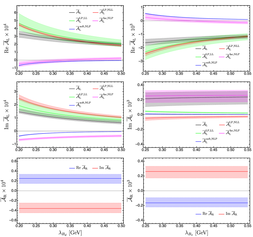
Figure 2: Breakdown of the distinct QCD mechanisms governing the two helicity amplitudes for $\bar{B}_{d}\to\gamma\gamma$ [left panel] and for $\bar{B}_{s}\to\gamma\gamma$ [right panel] with the theory uncertainties from the variations of the hard and hard-collinear scales in the default intervals.

We now proceed to explore the phenomenological impacts of the newly derived NLP corrections at ${\cal O}(\alpha_{s}^{0})$ and the NLL resummation improved leading power contributions on the exclusive radiative $B_{q}\to\gamma\gamma$ helicity amplitudes. To develop a transparent understanding of the higher order corrections from distinct dynamic mechanisms, we display in Figure 2 the $\lambda_{B_{q}}$ dependence of the leading power contributions at the LL and NLL accuracy, the combined local and non-local NLP corrections (107) from the QCD factorization approach and the subleading power soft contributions estimated with the dispersion technique for both $b\to d\,\gamma$ and $b\to s\,\gamma$ transitions, including the theory uncertainties from the variations of the hard scales $\mu_{\rm h}$ and $\nu$ as well as the hard-collinear scale $\mu$. Evidently, the radiative corrections with renormalization-group improvement can significantly reduce the perturbative scale uncertainties for the LL predictions of the helicity amplitude $\bar{\cal A}_{L}(\bar{B}_{q}\to\gamma\gamma)$ at leading power in the $\Lambda_{\rm QCD}/m_{b}$ expansion. In general, the perturbative QCD correction to ${\rm Re}\,\bar{\cal A}_{L}(\bar{B}_{q}\to\gamma\gamma)$ (with $q=d,\,s$) at ${\cal O}(\alpha_{s})$ can shift the corresponding LL prediction by an amount of approximately $(2\sim 10)\%$ for the allowed interval of $\lambda_{B_{q}}$ . Moreover, the yielding LL and NLL scale uncertainty bands only overlap marginally for ${\rm Im}\,\bar{\cal A}_{L}(\bar{B}_{d}\to\gamma\gamma)$ and even turn out to be well separated for ${\rm Im}\,\bar{\cal A}_{L}(\bar{B}_{s}\to\gamma\gamma)$, while adopting the central values for all the remaining input parameters. The latter can be attributed to the fact that the negligible LL contribution to ${\rm Im}\,\bar{\cal A}_{L}(\bar{B}_{s}\to\gamma\gamma)$ only arises from the heavily suppressed CKM factors ${\rm Im}\left[V_{ub}\,V_{us}^{\ast}\right]$ and ${\rm Im}\left[V_{cb}\,V_{cs}^{\ast}\right]$ in comparison with the counterpart amplitude ${\rm Re}\,\bar{\cal A}_{L}(\bar{B}_{s}\to\gamma\gamma)$, while the dominant NLL correction to ${\rm Im}\,\bar{\cal A}_{L}(\bar{B}_{s}\to\gamma\gamma)$ originating from the emerged strong phase of the two-loop contribution of the current-current operator $P_{2}^{c}$ is apparently free of such CKM suppression. In addition, the power suppressed soft corrections to both ${\rm Re}\,\bar{\cal A}_{L}(\bar{B}_{q}\to\gamma\gamma)$ and ${\rm Im}\bar{\cal A}_{L}(\bar{B}_{q}\to\gamma\gamma)$ will gives rise to the destructive interferences with the appropriate leading power contributions for the central input parameters, in analogy to the previous observation for $\bar{B}\to\gamma\ell\bar{\nu}_{\ell}$ [34, 35]. By contrast, the factorizable NLP correction to the amplitude ${\rm Re}\,\bar{\cal A}_{L}(\bar{B}_{q}\to\gamma\gamma)$ can flip the sign numerically with the evolution of the inverse moment $\lambda_{B_{q}}$ due to the nontrivial competing mechanisms between the two distinct sectors of $\{\bar{\cal A}_{L}^{A2,\,{\rm NLP}},\,\,\bar{\cal A}_{L}^{e_{b},\,{\rm NLP}},\,\,\bar{\cal A}_{L}^{\rm WA,\,NLP}\}$ and $\{\bar{\cal A}_{L}^{\rm hc,\,NLP},\,\,\bar{\cal A}_{L}^{m_{q},\,{\rm NLP}},\,\,\bar{\cal A}_{L}^{\rm HT,\,NLP}\}$ as displayed in Figure 3. However, the imaginary part of the factorizable NLP amplitude ${\rm Im}\,\bar{\cal A}_{L}^{\rm fac,\,NLP}(\bar{B}_{d}\to\gamma\gamma)$ will constantly lead to $(26\sim 35)\%$ reduction of the leading power contribution, because the overwhelming power corrections from $\{\bar{\cal A}_{L}^{\rm hc,\,NLP},\,\,\bar{\cal A}_{L}^{\rm HT,\,NLP},\,\,\bar{\cal A}_{L}^{\rm WA,\,NLP}\}$ remain as the negative quantities in the entire region of $\lambda_{B_{d}}\in[200,500]\,{\rm MeV}$. Furthermore, the major contribution to the subleading power amplitude ${\rm Im}\,\bar{\cal A}_{L}^{\rm fac,\,NLP}(\bar{B}_{s}\to\gamma\gamma)$ stems from the weak-annihilation type of the charm-loop diagrams generated by the four-quark operators $P_{1,2}^{c}$, as a result of the strong suppression of the remaining factorized NLP corrections from the weak phases of the CKM matrix elements entering the effective Hamiltonian of $b\to s\gamma$.

In addition, it has already become evident from the factorization formula (107) that the right-handed helicity amplitude $\bar{\cal A}_{R}(\bar{B}_{q}\to\gamma\gamma)$ results from the local subleading power contribution $\sum\limits_{i=1}^{6}\,C_{i}\,F_{i,R}^{(p),\,{\rm WA}}$ completely, in contrast to the large-recoil symmetry breaking effects for $\bar{B}_{q}\to\gamma\ell\bar{\ell}$ [41]. The sizeable uncertainties of the yielding predictions for ${\rm Re}\,\bar{\cal A}_{R}(\bar{B}_{q}\to\gamma\gamma)$ and ${\rm Im}\,\bar{\cal A}_{R}(\bar{B}_{q}\to\gamma\gamma)$ reflect the uncancelled renormalization-scale dependence of the Wilson coefficients $C_{i}(\nu)$ for the tree-level calculation described in Section 4.2, which is expected to be compensated by the unknown $\nu$-dependent hard functions at ${\cal O}(\alpha_{s})$ requiring the explicit evaluations of the two-loop one-particle irreducible diagrams depicted in Figure 4 of [14]. It needs to be pointed out further that the obtained results of ${\rm Re}\,\bar{\cal A}_{R}(\bar{B}_{d}\to\gamma\gamma)$ and ${\rm Im}\,\bar{\cal A}_{R}(\bar{B}_{d}\to\gamma\gamma)$ appear to own different signs from the counterpart predictions for $\bar{B}_{s}\to\gamma\gamma$ due to the contributing CKM matrix elements ${\rm Re}\,\left[V_{cb}\,V_{cd}^{\ast}\right]<0$ and ${\rm Re}\,\left[V_{cb}\,V_{cs}^{\ast}\right]>0$.

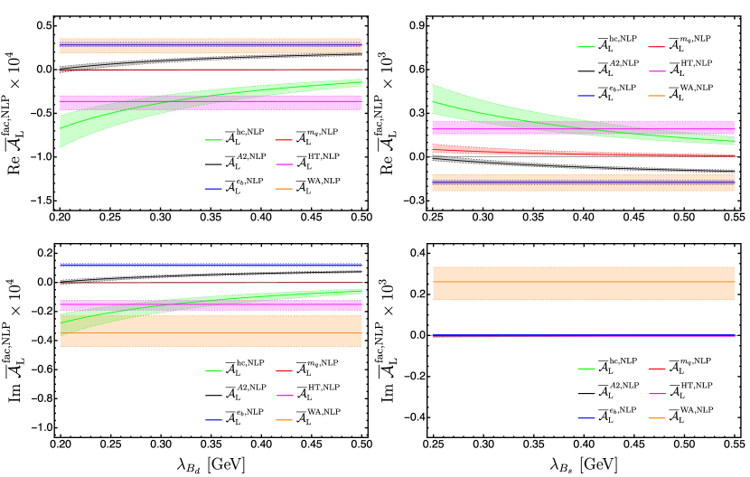
Figure 3: Theory predictions of the individual pieces yielding the subleading power corrections to the left-handed helicity amplitude in the heavy quark expansion for $\bar{B}_{d}\to\gamma\gamma$ [left panel] and for $\bar{B}_{s}\to\gamma\gamma$ [right panel] with the uncertainties from the variations of the hard and hard-collinear scales in the default intervals.

Inspecting the various NLP corrections to the factorizable $\bar{B}_{q}\to\gamma\gamma$ amplitudes displayed in Figure 3 numerically reveals the notable sensitivity of the real parts for $\bar{\cal A}_{L}^{\rm hc,\,NLP},\,\,\bar{\cal A}_{L}^{m_{q},\,{\rm NLP}}$ and $\bar{\cal A}_{L}^{A2,\,{\rm NLP}}$ on the actual value of $\lambda_{B_{q}}$, which together with the remaining NLP corrections independent of the inverse moment characterizes the diverse facets of the strong interaction dynamics encoded in the subleading power heavy-hadron decay amplitudes. It is also worth mentioning that the non-local strange-quark mass correction to ${\rm Re}\,\bar{\cal A}_{L}(\bar{B}_{s}\to\gamma\gamma)$ is of minor numerical importance when compared with the local subleading power effect from the (anti-)collinear photon radiation off the bottom quark in virtue of the smallness of the nonperturbative quantity $m_{s}/\lambda_{B_{s}}$ in reality. Thanks to the established CKM hierarchy [78]

$${\rm Im}\left[V_{tb}V_{td}^{\ast}\right]:{\rm Re}\left[V_{tb}V_{td}^{\ast}\right]=0.415:1\,,$$

adding the power suppressed helicity amplitudes ${\rm Im}\,\bar{\cal A}_{L}^{A2,\,\rm{NLP}}$ and ${\rm Im}\,\bar{\cal A}_{L}^{e_{b},\,\rm{NLP}}$ for the radiative $\bar{B}_{d}\to\gamma\gamma$ decay process together will fall short of the magnitude of the counterpart weak-annihilation contribution ${\rm Im}\,\bar{\cal A}_{L}^{\rm WA,\,NLP}$ consistently.

Figure 4: Theory predictions of the two helicity amplitudes for $\bar{B}_{d}\to\gamma\gamma$ [left panel] and for $\bar{B}_{s}\to\gamma\gamma$ [right panel] with the combined uncertainties by adding the separate errors due to the variations of all the input parameters collected in Section 6.1 in quadrature.

We further present in Figure 4 the final theory predictions for the helicity amplitudes of $\bar{B}_{q}\to\gamma\gamma$, as the analytical functions of the inverse moment $\lambda_{B_{q}}$, with the combined uncertainties by adding in quadrature all the separate uncertainties from varying the input parameters discussed in Section 6.1. It is straightforward to identify the dominant theory uncertainties for the left-handed helicity amplitudes arising from the hard and hard-collinear scale fluctuations and the inverse-logarithmic moments $\widehat{\sigma}_{B_{q}}^{(1)}$ and $\widehat{\sigma}_{B_{q}}^{(2)}$, in addition to the particular sensitivity to $\lambda_{B_{q}}$ . In contrast, the yielding theory uncertainties for the right-handed helicity amplitudes are dominated by the hard-scale variations of the Wilson coefficients $C_{i}(\nu)$ entering the tree-level factorization formulae of the weak-annihilation corrections. Moreover, our limited knowledge of the nonperturbative coefficient $X_{\rm NLP}$ parameterizing the rapidity divergence of the NLP correction (66) will not generate the sizeable uncertainty due to the smallness of the ratio $m_{q}/\lambda_{B_{q}}$ on top of the $\lambda_{B_{q}}/m_{B_{q}}$ suppression in comparison with the counterpart charmless two-body $B_{q}$-meson decays in QCD factorization [64].

6.3 Phenomenological observables for $B_{q}\to\gamma\gamma$

Prior to addressing the phenomenological implications of the improved calculations of the double radiative decay amplitudes on the experimental observables, we will construct the systematic expressions for investigating the CP-averaged branching fractions, the polarization fractions and the time-dependent CP asymmetries taking into account the neutral-meson mixing based upon the standard formalism presented in [78, 102]. In doing so, we are required to derive the decay amplitude for the counterpart channel $B_{q}\to\gamma\gamma$ by applying the CP-transformation for the amplitude (129)

$${\cal A}(B_{q}\to\gamma\gamma)=\left[-i\,{4\,G_{F}\over\sqrt{2}}\right]\,{\alpha_{\rm em}\over 4\pi}\,m_{B_{q}}^{3}\,\epsilon_{1}^{\ast\alpha}(p)\,\epsilon_{2}^{\ast\beta}(q)\,\,\left\{\sqrt{2}\,\left[-\,g_{\alpha\beta}^{\perp}\,{\cal A}_{\|}-i\,\varepsilon_{\alpha\beta}^{\perp}\,{\cal A}_{\perp}\right]\right\}\,,\hskip 22.76228pt$$ (156)

where we have adopted the phase convention ${\rm CP}\,|\bar{B}_{q}\rangle=-|B_{q}\rangle$ and the two transversity amplitudes ${\cal A}_{\|}$ and ${\cal A}_{\perp}$ can be determined from the corresponding “barred” amplitudes with all the weak phases conjugated. Solving the Schrödinger equation governing the time evolution of the $B_{q}-\bar{B}_{q}$ system immediately leads to the time-dependent decay rates [103, 104]

$$\Gamma^{\chi}(B_{q}(t)\to\gamma\,\gamma) = {\cal N}_{f}\,\left|{\cal A}^{\chi}(B_{q}\to\gamma\gamma)\right|^{2}\,\,{1+|\lambda_{f}^{\chi}|^{2}\over 2}\,{\rm exp}\left[-\Gamma_{q}\,t\right]\,\bigg{\{}\cosh{\Delta\Gamma_{q}\,t\over 2}+{\cal A}_{\Delta\Gamma}^{\chi}\,\sinh{\Gamma_{q}\,t\over 2}$$

$$\,+\,{\cal A}_{\rm CP}^{{\rm dir},\,\chi}\,\cos(\Delta m_{q}\,t)+{\cal A}_{\rm CP}^{{\rm mix},\,\chi}\,\sin(\Delta m_{q}\,t)\bigg{\}}\,,$$

$$\bar{\Gamma}^{\chi}(\bar{B}_{q}(t)\to\gamma\,\gamma) = {\cal N}_{f}\,\left|{\cal A}^{\chi}(B_{q}\to\gamma\gamma)\right|^{2}\,\,{1+|\lambda_{f}^{\chi}|^{2}\over 2}\,{{\rm exp}\left[-\Gamma_{q}\,t\right]\over 1-a_{q}}\,\bigg{\{}\cosh{\Delta\Gamma_{q}\,t\over 2}+{\cal A}_{\Delta\Gamma}^{\chi}\,\sinh{\Gamma_{q}\,t\over 2}$$ (157)

$$\,-\,{\cal A}_{\rm CP}^{{\rm dir},\,\chi}\,\cos(\Delta m_{q}\,t)-{\cal A}_{\rm CP}^{{\rm mix},\,\chi}\,\sin(\Delta m_{q}\,t)\bigg{\}}\,,$$

where ${\cal N}_{f}$ stands for the time-independent normalization factor arising from the phase-space integration and the index $\chi$ is introduced to characterize the parallel and perpendicular polarization configurations of the two-photon states. Apparently, the two decay amplitudes ${\cal A}^{\|}(B_{q}\to\gamma\gamma)$ and ${\cal A}^{\perp}(B_{q}\to\gamma\gamma)$ for the final states possessing the definite CP-parities can be obtained from (156) by keeping the individual terms proportional to ${\cal A}_{\|}$ and ${\cal A}_{\perp}$, respectively. The average width $\Gamma_{q}$ of the two bottom-meson mass eigenstates depends upon the diagonal matrix elements of the decay matrix with $\Gamma_{11}^{q}=\Gamma_{22}^{q}$ thanks to the CPT invariance of the effective Hamiltonian dictating the neutral-meson mixing pattern. The mass and width splittings between the light and heavy mass eigenstates can be expressed in terms of the dispersive and absorptive matrix elements $M_{12}^{q}$ and $\Gamma_{12}^{q}$. The $B_{q}$-mixing observables $\Delta m_{q}$ and $\Delta\Gamma_{q}$ further facilitate the construction of the two important quantities

$$x_{q}={\Delta m_{q}\over\Gamma_{q}}\,,\qquad y_{q}={\Delta\Gamma_{q}\over 2\,\Gamma_{q}}\,,$$ (158)

whose numerical results with uncertainties from the world average values of the experimental measurements [78] (with the combination procedures described in [105]) have been already summarized in Table 1. The small quantity $a_{q}$ characterizing the CP violation in mixing can be defined by the nondiagonal matrix elements in the following form

$$a_{q}=1-\left|{q\over p}\right|^{2}\,,\qquad{q\over p}=-\frac{\Delta m_{q}+i\,\Delta\Gamma_{q}/2}{2\,M_{12}^{q}-i\,\Gamma_{12}^{q}}=-\frac{2\,M_{12}^{q\,\ast}-i\,\Gamma_{12}^{q\,\ast}}{\Delta m_{q}+i\,\Delta\Gamma_{q}/2}\,.$$ (159)

The SM predictions for such flavour specific asymmetries [108, 107]

$$a_{d}=(-4.7\pm 0.6)\times 10^{-4}\,,\qquad a_{s}=(2.22\pm 0.27)\times 10^{-5}\,,$$ (160)

imply that we can safely drop out the tiny corrections of ${\cal O}(a_{q}^{n})$ (with $n\geq 1$) for the radiative $B_{q}\to\gamma\gamma$ decay phenomenology. The phase-convention independent combination $\lambda_{f}$ and the appearing three CP violation observables ${\cal A}_{\rm CP}^{{\rm dir},\,\chi}$, ${\cal A}_{\rm CP}^{{\rm mix},\,\chi}$ and ${\cal A}_{\Delta\Gamma}^{\chi}$ are further defined as

$$\lambda_{f}^{\chi}={q\over p}\,\frac{\bar{\cal A}^{\chi}(\bar{B}_{q}\to\gamma\gamma)}{{\cal A}^{\chi}(B_{q}\to\gamma\gamma)}\,, {\cal A}_{\rm CP}^{{\rm dir},\,\chi}=\frac{1-|\lambda_{f}^{\chi}|^{2}}{1+|\lambda_{f}^{\chi}|^{2}}\,,$$

$${\cal A}_{\rm CP}^{{\rm mix},\,\chi}=-\frac{2\,{\rm Im}\,\lambda_{f}^{\chi}}{1+|\lambda_{f}^{\chi}|^{2}}\,, {\cal A}_{\Delta\Gamma}^{\chi}=-\frac{2\,{\rm Re}\,\lambda_{f}^{\chi}}{1+|\lambda_{f}^{\chi}|^{2}}\,,$$ (161)

which evidently reveals an exact relation

$$|{\cal A}_{\rm CP}^{{\rm dir},\,\chi}|^{2}+|{\cal A}_{\rm CP}^{{\rm mix},\,\chi}|^{2}+|{\cal A}_{\Delta\Gamma}^{\chi}|^{2}=1\,.$$ (162)

Expanding the obtained expression (159) for the phase-convention dependent quantity $q/p$ in terms of the small parameter $|\Gamma_{12}^{q}/M_{12}^{q}|$ leads to an approximate solution [106]

$${q\over p}=-{M_{12}^{q\,\ast}\over|M_{12}^{q}|}\,\left[1-{a_{q}\over 2}\right]+{\cal O}\left(\left|{\Gamma_{12}^{q}\over M_{12}^{q}}\right|^{2}\right)\,.$$ (163)

The SM contributions of the off-diagonal matrix element $M_{12}^{q}$ turn out to be dominated by the $\Delta B=2$ box diagrams with internal top and anti-top quarks due to the very strong GIM cancellation [109] for the yielding two terms proportional to $\lambda_{c}^{2}$ and $\lambda_{c}\,\lambda_{t}$ (with $\lambda_{p}=V_{pb}\,V_{pq}^{\ast}$), which can be traced back to the peculiar analytical behaviours of the associated perturbative loop function $F\left(m_{p_{1}}^{2}/m_{W}^{2},m_{p_{2}}^{2}/m_{W}^{2}\right)$ [110, 107]. We are then led to conclude that the imaginary part of $M_{12}^{q}$ originates to a rather good approximation from the CKM factor $V_{tb}\,V_{tq}^{\ast}$ uniquely with the standard OPE technique, which further enables us to write down an even illuminating relation for the $B_{q}$-meson mixing

$${q\over p}\simeq-\frac{V_{tb}^{\ast}\,V_{tq}}{V_{tb}\,V_{tq}^{\ast}}=-{\rm exp}\left[i\,{\rm arg}(V_{tb}^{\ast}\,V_{tq})^{2}\right]\,.$$ (164)

According to (157), we can immediately derive the CP-averaged branching fraction of $B_{q}\to\gamma\gamma$ for the flavour-tagged measurement at an $e^{+}\,e^{-}$ collider with equal numbers of the produced bottom and anti-bottom mesons [112, 111]

$${\cal BR}^{\chi}(B_{q}\to\gamma\gamma) = {\cal N}_{f}\,\left|{\cal A}^{\chi}(B_{q}\to\gamma\gamma)\right|^{2}\,{1+|\lambda_{f}^{\chi}|^{2}\over 2}\,\int_{-\infty}^{+\infty}dt\,\,{\rm exp}\left[-\Gamma_{q}\,|t|\right]\,$$ (165)

$$\,\times\,\left\{\cosh{\Delta\Gamma_{q}\,t\over 2}+{\cal A}_{\Delta\Gamma}^{\chi}\,\sinh{\Gamma_{q}\,t\over 2}\right\}+{\cal O}(a_{q})$$

$$= \left({{\cal N}_{f}\over\Gamma_{q}}\right)\,\left|{\cal A}^{\chi}(B_{q}\to\gamma\gamma)\right|^{2}\,\left(1+|\lambda_{f}^{\chi}|^{2}\right)\,\left({1\over 1-y_{q}^{2}}\right)+{\cal O}(a_{q})\,$$

$$= \langle{\cal BR}^{\chi}(B_{q}\to\gamma\gamma)\rangle_{\rm th}\,\left({1\over 1-y_{q}^{2}}\right)+{\cal O}(a_{q})\,.$$

Interestingly, the resulting correction factor of the time-integrated branching ratio due to the neutral-meson mixing is independent of the polarization index $\chi$ for the coherent bottom-meson pair production at the SuperKEKB accelerator. The CP-averaged branching fraction in the limit $\Delta\Gamma_{q}\to 0$ can be readily computed from the corresponding transversity amplitudes

$$\langle{\cal BR}^{\chi}(B_{q}\to\gamma\gamma)\rangle_{\rm th}={\tau_{B_{q}}\over 2}\,\frac{\alpha_{\rm em}^{2}\,G_{F}^{2}\,m_{B_{q}}^{5}}{16\,\pi^{3}}\,\left(|{\cal A}_{\chi}|^{2}+|\bar{\cal A}_{\chi}|^{2}\right)\,.$$ (166)

Consequently, we can proceed to construct a typical set of phenomenological observables in analogy to the two-body hadronic $B\to VV$ decays [42]

$${\cal BR}(B_{q}\to\gamma\gamma)=\sum_{\chi=\|,\,\perp}\,{\cal BR}^{\chi}(B_{q}\to\gamma\gamma)\,,\qquad f_{\chi}=\frac{{\cal BR}^{\chi}(B_{q}\to\gamma\gamma)}{{\cal BR}(B_{q}\to\gamma\gamma)}\,,$$ (167)

where the two polarization fractions are apparently not linearly independent due to the normalization condition $f_{\|}\,+\,f_{\perp}=1$. Applying the definition for the time-dependent CP asymmetry for the neutral $B_{q}$-meson decaying into CP eigenstates yields [102]

$$A_{\rm CP}^{\chi}(t) = \frac{\bar{\Gamma}^{\chi}(\bar{B}_{q}(t)\to\gamma\gamma)-\Gamma^{\chi}(B_{q}(t)\to\gamma\gamma)}{\bar{\Gamma}^{\chi}(\bar{B}_{q}(t)\to\gamma\gamma)+\Gamma^{\chi}(B_{q}(t)\to\gamma\gamma)}$$ (168)

$$= -\frac{{\cal A}_{\rm CP}^{{\rm dir},\,\chi}\,\cos(\Delta m_{q}\,t)+{\cal A}_{\rm CP}^{{\rm mix},\,\chi}\,\sin(\Delta m_{q}\,t)}{\cosh(\Delta\Gamma_{q}\,t/2)+{\cal A}_{\Delta\Gamma}^{\chi}\,\sinh(\Delta\Gamma_{q}\,t/2)}\,.$$

The quantity ${\cal A}_{\rm CP}^{{\rm dir},\,\chi}$ describes the direct CP-violating effect as a consequence of $\left|\bar{\cal A}^{\chi}:{\cal A}^{\chi}\right|\neq 1$, which requires the appearance of at least two individual terms with distinct strong and weak phases simultaneously contributing to the transversity amplitude ${\cal A}^{\chi}$. By contrast, ${\cal A}_{\rm CP}^{{\rm mix},\,\chi}$ encodes the CP-violating information due to interference between decays with and without mixing for the final states common to both the bottom and anti-bottom meson decays (i.e., by virtue of the two different decay mechanisms of $B_{q}\to\gamma\gamma$ and $B_{q}\to\bar{B}_{q}\to\gamma\gamma$). The observable ${\cal A}_{\Delta\Gamma}^{\chi}$ takes the extreme values $\pm 1$ for the so-called “golden modes” with CP-eigenstate final states, whose decay amplitudes contain only one CKM structure such that $|\lambda_{f}^{\chi}|=1$.

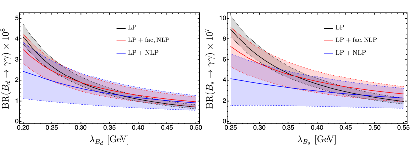
Figure 5: Theory predictions for the $\lambda_{B_{q}}$-dependence of the CP-averaged branching fractions of $\bar{B}_{d}\to\gamma\gamma$ [left panel] and $\bar{B}_{s}\to\gamma\gamma$ [right panel], where the numerical results obtained with the NLL resummation improved leading power approximations [grey bands] and with adding further solely the factorizable NLP corrections [red bands] are also shown for a comparison.

We now present the improved theory predictions for the CP-averaged branching fractions of $B_{q}\to\gamma\gamma$ in the presence of the neutral-meson mixing in Figure 5, which summarizes our main phenomenological results for confronting the forthcoming precision Belle II measurements with an ultimate integrated luminosity of $50\,{\rm ab}^{-1}$ [15]. The factorizable NLP correction to ${\cal BR}(B_{q}\to\gamma\gamma)$ appears to reduce the counterpart leading power contribution by approximately an amount of $(15-20)\,\%$ at $\lambda_{B_{d}}=200\,{\rm MeV}$ ($\lambda_{B_{s}}=250\,{\rm MeV}$). However, such destructive interference mechanism will gradually evolve into the constructive intervention pattern with the increase of $\lambda_{B_{q}}$ (as large as $35\,\%$ enhancement at the maximal value of the inverse moment) due to the emergence of the zero-crossing regime for the factorizable NLP correction to the amplitude ${\rm Re}\,\bar{\cal A}_{L}(\bar{B}_{q}\to\gamma\gamma)$ as discussed in Section 6.2 together with the hierarchy structure

$$|{\rm Re}\,\bar{\cal A}_{L}(\bar{B}_{q}\to\gamma\gamma)|:|{\rm Im}\,\bar{\cal A}_{L}(\bar{B}_{q}\to\gamma\gamma)|\in[2.3,3.3]\,,$$

$$|{\rm Re}\,\bar{\cal A}_{L}(\bar{B}_{s}\to\gamma\gamma)|:|{\rm Im}\,\bar{\cal A}_{L}(\bar{B}_{s}\to\gamma\gamma)|\in[5.5,7.6]\,,$$ (169)

where the quoted uncertainties arise from the variations of $\lambda_{B_{q}}$ merely. The NLP resolved photon contribution to the branching fraction of $B_{q}\to\gamma\gamma$ will result in the sizeable reduction of the corresponding “${\rm LP+fac,\,NLP}$” prediction with the default ansatz of the $B_{q}$-meson distribution amplitude (131) at $\alpha=\beta$ (namely, the exponential model [48, 30, 71]): numerically $(6-28)\,\%$ and $(15-43)\,\%$ corrections for $b\to d\,\gamma$ and $b\to s\,\gamma$ transitions, respectively. Inspecting the distinct sources of the yielding theory uncertainties as collected in Tables 2 and 3, the currently poor understanding towards the two-particle and three-particle $B_{q}$-meson distribution amplitudes in HQET remains the most significant ingredient of preventing us from achieving the phenomenologically encouraging precision up to date, which can be competitive with the experimental prospects of the anticipated Belle II measurements (with the estimated precision of $9.6\,\%$ and $23\,\%$ for ${\cal BR}(B_{d}\to\gamma\gamma)$ and ${\cal BR}(B_{s}\to\gamma\gamma)$ approximately).

	Central Value	Total Error	$\lambda_{B_{d}}$	$\{\widehat{\sigma}_{B_{d}}^{(1)},\,\widehat{\sigma}_{B_{d}}^{(2)}\}$	$\mu$	$\nu$	$\mu_{\rm h}$	$\bar{\Lambda}$	$m^{\rm PS}_{c}$
$10^{8}\times{\cal BR}$	1.352	${}_{-0.745}^{+1.242}$	${}_{-0.439}^{+1.091}$	${}_{-0.516}^{+0.503}$	${}_{-0.127}^{+0.032}$	${}_{-0.245}^{+0.235}$	${}_{-0.051}^{+0.167}$	${}_{-0.110}^{+0.098}$	${}_{-0.030}^{+0.030}$
$f_{\|}$	0.386	${}_{-0.058}^{+0.060}$	${}_{-0.030}^{+0.033}$	${}_{-0.038}^{+0.019}$	${}_{-0.007}^{+0.001}$	${}_{-0.030}^{+0.044}$	${}_{-0.003}^{+0.008}$	${}_{-0.006}^{+0.005}$	${}_{-0.002}^{+0.002}$
$f_{\perp}$	0.614	${}_{-0.060}^{+0.058}$	${}_{-0.033}^{+0.030}$	${}_{-0.019}^{+0.038}$	${}_{-0.001}^{+0.007}$	${}_{-0.044}^{+0.030}$	${}_{-0.008}^{+0.003}$	${}_{-0.005}^{+0.006}$	${}_{-0.002}^{+0.002}$
${\cal A}^{\rm dir,\,\|}_{\rm CP}$	0.130	${}_{-0.027}^{+0.044}$	${}_{-0.007}^{+0.012}$	${}_{-0.010}^{+0.016}$	${}_{-0.006}^{+0.008}$	${}_{-0.019}^{+0.029}$	${}_{-0.012}^{+0.024}$	${}_{-0.005}^{+0.006}$	${}_{-0.004}^{+0.004}$
${\cal A}^{\rm mix,\,\|}_{\rm CP}$	$-0.155$	${}_{-0.060}^{+0.036}$	${}_{-0.016}^{+0.009}$	${}_{-0.022}^{+0.013}$	${}_{-0.011}^{+0.008}$	${}_{-0.039}^{+0.025}$	${}_{-0.032}^{+0.016}$	${}_{-0.008}^{+0.006}$	${}_{-0.008}^{+0.008}$
${\cal A}^{\|}_{\Delta\Gamma}$	$-0.979$	${}_{-0.009}^{+0.017}$	${}_{-0.002}^{+0.004}$	${}_{-0.003}^{+0.006}$	${}_{-0.002}^{+0.003}$	${}_{-0.006}^{+0.011}$	${}_{-0.004}^{+0.009}$	${}_{-0.002}^{+0.002}$	${}_{-0.002}^{+0.002}$
${\cal A}^{\rm dir,\,\perp}_{\rm CP}$	0.356	${}_{-0.063}^{+0.076}$	${}_{-0.037}^{+0.030}$	${}_{-0.038}^{+0.061}$	${}_{-0.008}^{+0.017}$	${}_{-0.023}^{+0.010}$	${}_{-0.009}^{+0.015}$	${}_{-0.011}^{+0.014}$	${}_{-0.019}^{+0.019}$
${\cal A}^{\rm mix,\,\perp}_{\rm CP}$	0.083	${}_{-0.058}^{+0.079}$	${}_{-0.034}^{+0.041}$	${}_{-0.026}^{+0.008}$	${}_{-0.003}^{+0.000}$	${}_{-0.037}^{+0.061}$	${}_{-0.012}^{+0.028}$	${}_{-0.001}^{+0.000}$	${}_{-0.007}^{+0.007}$
${\cal A}^{\perp}_{\Delta\Gamma}$	0.931	${}_{-0.030}^{+0.019}$	${}_{-0.009}^{+0.009}$	${}_{-0.024}^{+0.013}$	${}_{-0.007}^{+0.003}$	${}_{-0.001}^{+0.001}$	${}_{-0.009}^{+0.004}$	${}_{-0.005}^{+0.004}$	${}_{-0.008}^{+0.008}$

Table 2: Theory predictions of the CP-averaged branching fraction, the two polarization fractions and the six CP-violating observables for $B_{d}\to\gamma\gamma$ in the presence of the neutral-meson mixing with the total uncertainties obtained by adding all separate uncertainties in quadrature, where the numerically important individual uncertainties for each physical quantity are further displayed for completeness.

	Central Value	Total Error	$\lambda_{B_{s}}$	$\{\widehat{\sigma}_{B_{s}}^{(1)},\,\widehat{\sigma}_{B_{s}}^{(2)}\}$	$\mu$	$\nu$	$\mu_{\rm h}$	$\bar{\Lambda}$	$m^{\rm PS}_{c}$
$10^{7}\times{\cal BR}$	2.964	${}_{-1.614}^{+1.800}$	${}_{-0.671}^{+1.173}$	${}_{-1.163}^{+1.071}$	${}_{-0.421}^{+0.164}$	${}_{-0.709}^{+0.672}$	${}_{-0.114}^{+0.358}$	${}_{-0.272}^{+0.258}$	${}_{-0.077}^{+0.076}$
$f_{\|}$	0.361	${}_{-0.065}^{+0.064}$	${}_{-0.024}^{+0.026}$	${}_{-0.047}^{+0.023}$	${}_{-0.013}^{+0.004}$	${}_{-0.033}^{+0.052}$	${}_{-0.004}^{+0.010}$	${}_{-0.008}^{+0.006}$	${}_{-0.003}^{+0.003}$
$f_{\perp}$	0.639	${}_{-0.064}^{+0.065}$	${}_{-0.026}^{+0.024}$	${}_{-0.023}^{+0.047}$	${}_{-0.004}^{+0.013}$	${}_{-0.052}^{+0.033}$	${}_{-0.010}^{+0.004}$	${}_{-0.006}^{+0.008}$	${}_{-0.003}^{+0.003}$
$10^{2}\times{\cal A}^{\rm dir,\,\|}_{\rm CP}$	$-0.635$	${}_{-0.249}^{+0.151}$	${}_{-0.084}^{+0.048}$	${}_{-0.098}^{+0.055}$	${}_{-0.048}^{+0.034}$	${}_{-0.162}^{+0.102}$	${}_{-0.119}^{+0.060}$	${}_{-0.036}^{+0.030}$	${}_{-0.018}^{+0.019}$
$10^{2}\times{\cal A}^{\rm mix,\,\|}_{\rm CP}$	0.763	${}_{-0.198}^{+0.338}$	${}_{-0.063}^{+0.114}$	${}_{-0.072}^{+0.132}$	${}_{-0.045}^{+0.064}$	${}_{-0.133}^{+0.221}$	${}_{-0.078}^{+0.161}$	${}_{-0.039}^{+0.048}$	${}_{-0.040}^{+0.040}$
$10^{4}\times\left({\cal A}^{\|}_{\Delta\Gamma}+1\right)$	0.493	${}_{-0.230}^{+0.459}$	${}_{-0.076}^{+0.150}$	${}_{-0.085}^{+0.176}$	${}_{-0.055}^{+0.082}$	${}_{-0.152}^{+0.310}$	${}_{-0.093}^{+0.218}$	${}_{-0.047}^{+0.062}$	${}_{-0.042}^{+0.043}$
$10^{2}\times{\cal A}^{\rm dir,\,\perp}_{\rm CP}$	$-1.888$	${}_{-0.409}^{+0.273}$	${}_{-0.072}^{+0.059}$	${}_{-0.342}^{+0.201}$	${}_{-0.124}^{+0.062}$	${}_{-0.024}^{+0.074}$	${}_{-0.077}^{+0.046}$	${}_{-0.085}^{+0.071}$	${}_{-0.113}^{+0.109}$
$10^{2}\times{\cal A}^{\rm mix,\,\perp}_{\rm CP}$	$-0.273$	${}_{-0.426}^{+0.318}$	${}_{-0.192}^{+0.148}$	${}_{-0.066}^{+0.185}$	${}_{-0.000}^{+0.031}$	${}_{-0.343}^{+0.195}$	${}_{-0.141}^{+0.060}$	${}_{-0.010}^{+0.014}$	${}_{-0.024}^{+0.022}$
$10^{4}\times\left(A^{\perp}_{\Delta\Gamma}-1\right)$	$-1.820$	${}_{-0.802}^{+0.456}$	${}_{-0.108}^{+0.039}$	${}_{-0.671}^{+0.338}$	${}_{-0.234}^{+0.117}$	${}_{-0.015}^{+0.000}$	${}_{-0.197}^{+0.100}$	${}_{-0.160}^{+0.129}$	${}_{-0.228}^{+0.205}$

Table 3: Theory predictions of the CP-averaged branching fraction, the two polarization fractions and the six CP-violating observables for $B_{s}\to\gamma\gamma$ in the presence of the neutral-meson mixing with the total uncertainties obtained by adding all separate uncertainties in quadrature, where the numerically important individual uncertainties for each physical quantity are further displayed for completeness.

Remarkably, including the subleading power soft corrections to the time-integrated decay rates will enlarge the combined theory uncertainties by almost a factor of two for both exclusive radiative decay processes with the central values of $\lambda_{B_{q}}$, which can be attributed to the even more pronounced sensitivity to the shape parameters $\widehat{\sigma}_{B_{d}}^{(1)}$ and $\widehat{\sigma}_{B_{d}}^{(2)}$ under this circumstance. We can readily understand such interesting observation from the fact that the two inverse-logarithmic moments will start to emerge in the leading power factorization formulae for the helicity amplitudes by means of either the perturbative correction to the hard-collinear matching coefficient or the renormalization-group evolution of the inverse moment $\lambda_{B_{q}}$, both of which will lead to an effective suppression factor $\alpha_{s}(\mu)\,C_{F}/(4\,\pi)\approx 0.04$ at $\mu=1.5\,{\rm GeV}$ numerically. On the contrary, the NLP resolved photon contribution (122) estimated with the dispersion approach depends on the functional form (particularly the small-$\omega$ behaviour) of the leading twist $B_{q}$-meson distribution amplitude $\phi_{B}^{+}(\omega,\,\mu)$ already at tree level (see [93, 114] for earlier discussions in the context of the heavy-to-light decay form factors). A number of important comments on the numerical results presented in Tables 2 and 3 are in order.

• It is instructive to derive the transparent expression of the ratio for the two branching fractions of $B_{q}\to\gamma\gamma$ in the leading-order approximation of the double expansion in powers of $\Lambda/m_{b}$ and $\alpha_{s}$

  $$\frac{{\cal BR}(B_{s}\to\gamma\gamma)}{{\cal BR}(B_{d}\to\gamma\gamma)} = {\tau_{B_{s}}\over\tau_{B_{d}}}\,\left|{V_{ts}\over V_{td}}\right|^{2}\,\left({m_{B_{s}}\over m_{B_{d}}}\right)^{3}\,\left({f_{B_{s}}\over f_{B_{d}}}\right)^{2}\,\left({\lambda_{B_{d}}\over\lambda_{B_{s}}}\right)^{2}\,\left({1-y_{d}^{2}\over 1-y_{s}^{2}}\right)+{\cal O}\left({\Lambda\over m_{b}},\alpha_{s}\right)$$ (170)

  $$= 33.80\,\left({\lambda_{B_{d}}\over\lambda_{B_{s}}}\right)^{2}+{\cal O}\left({\Lambda\over m_{b}},\alpha_{s}\right)\,.$$

  We have verified explicitly that the $\lambda_{B_{q}}$-scaling violation effect at leading power in the heavy quark expansion appears to be insignificant numerically (at the level of ${\cal O}(1\,\%)$); while the subleading power factorizable and soft contributions can result in approximately $(10-20)\,\%$ corrections to the scaling behaviour (170) for the default intervals of the two inverse moments. It is therefore of high interest to carry out the precision measurements for such “golden observable” ${\cal BR}(B_{s}\to\gamma\gamma):{\cal BR}(B_{d}\to\gamma\gamma)$ at the Belle II experiment, which allow for an excellent determination of the ratio of the two inverse moments with the systematic theory uncertainties at the level of $(5-10)\,\%$ in the leading-power approximation.

• In comparison with the previous predictions of the exclusive radiative $B_{q}\to\gamma\gamma$ decay rates from the QCD factorization approach [16]

  $${\cal BR}(B_{d}\to\gamma\gamma)\big{|}_{\rm DS}\simeq 3\times 10^{-8}\,,\qquad{\cal BR}(B_{s}\to\gamma\gamma)\big{|}_{\rm DS}\simeq 10^{-6}\,,$$ (171)

  our numerical results for the corresponding leading power contributions with the central values of the input parameters turn out to be smaller by a factor of $2-3$ approximately. The observed discrepancies in large part stem from approximating the $\overline{\rm MS}$-mass of the $b$-quark by the bottom-meson mass for the resulting hard-scattering kernel (19) in [16], from adopting the higher value of the effective Wilson coefficient $C_{7}^{\rm eff}(4.8\,{\rm GeV})=-0.390$ and from taking the lower value of the inverse moment for the $B_{s}$-meson distribution amplitude $\lambda_{B_{s}}(\mu_{0})=350\,{\rm MeV}$ implemented in the phenomenological analysis of [16].

• Adding the factorizable NLP weak-annihilation correction on the top of the leading-power contribution from the magnetic penguin operator $P_{7}$ and adopting further the central input parameters gives rise to [14]

  $${\cal BR}(B_{d}\to\gamma\gamma)\big{|}_{\rm BB}=3.11\times 10^{-8}\,,\qquad{\cal BR}(B_{s}\to\gamma\gamma)\big{|}_{\rm BB}=1.23\times 10^{-6}\,,$$ (172)

  which differ prominently from our numerical predictions with the same theory accuracy

  $${\cal BR}(B_{d}\to\gamma\gamma)=1.78\times 10^{-8}\,,\qquad{\cal BR}(B_{s}\to\gamma\gamma)=3.88\times 10^{-7}\,.$$ (173)

  The dominating mechanisms accounting for the notable differences between (172) and (173) lie in the replacement of the $\overline{\rm MS}$-scheme bottom-quark mass in the effective weak operator $P_{7}$ by the counterpart heavy-meson mass $m_{B_{q}}$ for deriving the leading-power transversity amplitudes (3.2) in [14], which invokes additionally the approximate SU(3)-flavour symmetry relation $\lambda_{B_{s}}=\lambda_{B_{d}}$ in the numerical extrapolation.

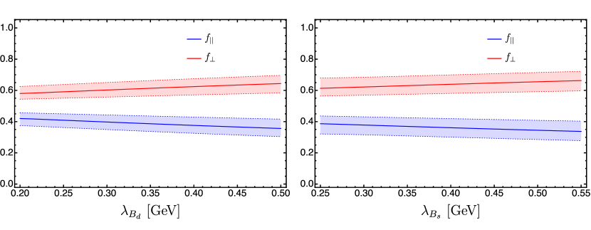
Figure 6: Theory predictions for the $\lambda_{B_{q}}$-dependence of the CP-averaged polarization fractions of $\bar{B}_{d}\to\gamma\gamma$ [left panel] and $\bar{B}_{s}\to\gamma\gamma$ [right panel].

We proceed to present our predictions for the polarization fractions of the double radiative $B_{q}$-meson decays within the default intervals of the inverse moments in Figure 6. Apparently, the yielding uncertainties for such ratio observables are substantially improved, when compared with the numerical results of the CP-averaged branching fractions displayed in (5), thanks to the striking cancellation of the errors from varying the shape parameters of the bottom-meson distribution amplitudes. The most significant uncertainties for the polarization fractions arise from the variations of QCD renormalization scale $\nu$ as shown in Tables 2 and 3. It is appropriate to emphasize that the deviation of the quantity $f_{\|}:f_{\perp}$ from one evidently characterizes the typical size of the subleading power correction in the $\Lambda_{\rm QCD}/m_{b}$ expansion. In addition, the SU(3)-flavour symmetry violation effects for the polarization fractions are estimated to be extraordinary small, around $(4-7)\,\%$ numerically, on account of an extra suppression factor from the heavy quark mass expansion.

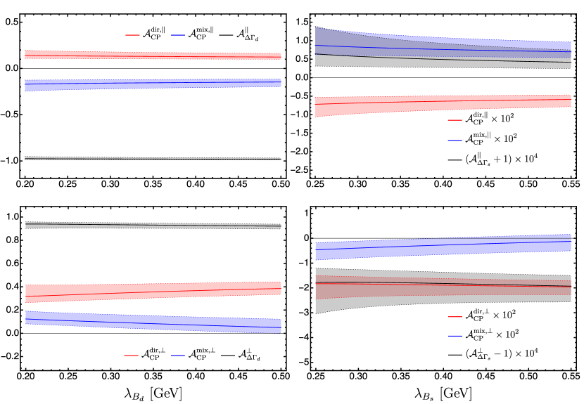
Figure 7: Theory predictions for the $\lambda_{B_{q}}$-dependence of the three observables ${\cal A}_{\rm CP}^{{\rm dir},\,\chi}$, ${\cal A}_{\rm CP}^{{\rm mix},\,\chi}$ and ${\cal A}_{\Delta\Gamma_{q}}^{\chi}$ (with $\chi=\|,\perp$) determining the time-dependent CP asymmetries of of $\bar{B}_{d}\to\gamma\gamma$ [left panel] and $\bar{B}_{s}\to\gamma\gamma$ [right panel] in the approximation of discarding the negligible CP violation in mixing.

Finally we turn to display in Figure 7 the theory predictions for the three observables determining the time-dependent CP asymmetries of $B_{q}\to\gamma\gamma$ with the nonvanishing width splittings $\Delta\Gamma_{q}$. The apparent hierarchy structure for the CKM matrix elements contributing to the $B_{s}\to\gamma\,\gamma$ helicity amplitudes

$$|V_{ub}\,V_{us}^{\ast}|:|V_{cb}\,V_{cs}^{\ast}|\approx 1:50\,,$$ (174)

indicates the model-independent results of the mass-eigenstate rate asymmetries ${\cal A}_{\Delta\Gamma}^{\|}\simeq-1$ and ${\cal A}_{\Delta\Gamma}^{\perp}\simeq+1$ by dropping out the negligible $V_{ub}\,V_{us}^{\ast}$ terms in (125), which are further supported by the complete NLL QCD calculations at leading power in $\Lambda_{\rm QCD}/m_{b}$ with the various NLP corrections at tree level as summarized in Table 3. The yielding predictions for ${\cal A}_{\rm CP}^{\rm dir,\,\|}$, ${\cal A}_{\rm CP}^{\rm mix,\,\|}$ and ${\cal A}_{\rm CP}^{\rm dir,\,\perp}$ suffer from the relatively smaller uncertainties than the counterpart results for the CP-averaged branching fractions. By contrast, the resulting values of ${\cal A}_{\rm CP}^{\rm mix,\,\perp}$ collected in Tables 2 and 3 appear to be more uncertain, mainly from varying the inverse moment $\lambda_{B_{q}}$ as well as the perturbative hard scale $\nu$. According to the definition of ${\cal A}_{\rm CP}^{\rm mix,\,\perp}$ in (161), we can readily identify the emerged considerable uncertainties from the strong sensitivity of the Wilson-coefficient combination $\left[C_{F}\,C_{1}(\nu)+C_{2}(\nu)\right]$ entering the factorizable weak-annihilation amplitude ${\cal F}_{V}^{(p),\,\rm WA}$ in (104) on the renormalization scale $\nu$. As can be understood from the factorization formula (45), the two direct CP-violating quantities ${\cal A}_{\rm CP}^{\rm dir,\,\|}$ and ${\cal A}_{\rm CP}^{\rm dir,\,\perp}$ are expected to be identical in the leading-power approximation. However, the obtained numerical results displayed in Tables 2 and 3 tend to suggest that the subleading power contributions to the radiative $B_{q}$-meson decay amplitudes in the heavy quark expansion can numerically generate the substantial corrections to the above-mentioned asymptotic scaling. This pattern can be attributed to the fact that the higher order terms in the heavy quark mass expansion will generally lead to the enormous impacts on the perturbative strong phases for the exclusive $B_{q}$-decay amplitudes due to the absence of the $\alpha_{s}$ suppression.

7 Conclusions

In the present paper we have carried out the improved calculations of the double radiative $B_{q}$-meson decay amplitudes beyond the leading-power accuracy by taking advantage of the perturbative factorization technique and the dispersion approach. The NLO hard matching coefficients from the two-loop QCD matrix elements of $\langle q\,\gamma|H_{\rm eff}|b\rangle$ including the QCD penguin operators $P_{3,...,6}$ were taken into account for the first time based upon the analytical calculations performed in [17], which are apparently of importance for exploring the phenomenological observables of $B_{d}\to\gamma\,\gamma$. A complete NLL resummation for the enhanced logarithms of $m_{b}/\Lambda_{\rm QCD}$ appearing in the SCET factorization formula for the radiative $B_{q}\to\gamma\,\gamma$ decay amplitude has been accomplished with the renormalization group formalism in momentum space. Subsequently, we constructed the factorized expressions for the NLP contributions from the non-local hard-collinear interaction due to the energetic photon radiation off the light-flavour quark of the bottom meson, from the nonvanishing light-quark mass, from the subleading power heavy-to-light current $J^{(\rm A2)}$ in SCET, from the two-particle and three-particle $B_{q}$-meson distribution amplitudes up to the twist-six accuracy, from the (anti)-collinear photon emission from the bottom quark and from the one-particle irreducible weak-annihilation diagrams at tree level in detail in Section 4. It is remarkable to mention that all the above-mentioned non-local NLP corrections other than the light-quark mass effect (63) can be expressed in terms of the convolution integrals of the hard-collinear functions and the HQET distribution amplitudes free of the potential rapidity divergences, which would invalidate the resulting soft-collinear factorization formulae otherwise. We further evaluated the NLP resolved photon contribution to the two helicity form factors with the OPE-controlled dispersion technique at ${\cal O}(\alpha_{s})$. The large-recoil symmetry violating effect between the two transversity amplitudes has proven to be solely generated by the local NLP contribution by means of the weak-annihilation mechanism.

Adopting the three-parameter ansatz for the essential $B_{q}$-meson distribution amplitudes [35] fulfilling the classical equation-of-motion constraints and the appropriate asymptotic behaviors at small quark and gluon momenta, we have investigated the numerical implications of the newly derived theory ingredients on the $B_{q}\to\gamma\gamma$ decay phenomenology systematically in Section 6. The attractive advantage of implementing this nonperturbative LCDA model for the nonlocal NLP contributions consists in the complete independence of the yielding factorized results on the very profile function $f(\omega)$ parameterizing the leading-twist $B_{q}$-meson distribution amplitude as presented in (150), (6.1), (152), (153) and (154). The NLL QCD corrections to the leading power predictions of the helicity amplitudes ${\rm Re}\,\bar{\cal A}_{L}(\bar{B}_{q}\to\gamma\gamma)$ have been estimated to be in the range of $(2-10)\%$ for $\lambda_{B_{d}}=(350\pm 50)\,{\rm MeV}$ and $\lambda_{B_{s}}=(400\pm 50)\,{\rm MeV}$. On the other hand, the factorizable NLP contributions to ${\rm Re}\,\bar{\cal A}_{L}(\bar{B}_{q}\to\gamma\gamma)$ appeared to flip the sign numerically with the growing value of the inverse moment $\lambda_{B_{q}}$ due to the intrinsic competitions between the two different sectors of $\{\bar{\cal A}_{L}^{A2,\,{\rm NLP}},\,\,\bar{\cal A}_{L}^{e_{b},\,{\rm NLP}},\,\,\bar{\cal A}_{L}^{\rm WA,\,NLP}\}$ and $\{\bar{\cal A}_{L}^{\rm hc,\,NLP},\,\,\bar{\cal A}_{L}^{m_{q},\,{\rm NLP}},\,\,\bar{\cal A}_{L}^{\rm HT,\,NLP}\}$; and the resulting correction factors could reach an amount of ${\cal O}(15\,\%)$ in magnitude maximally. In particular, the factorizable NLP corrections to the imaginary part of the helicity amplitude ${\rm Im}\,\bar{\cal A}_{L}(\bar{B}_{d}\to\gamma\gamma)$ turned out to be even more pronounced: as large as $(26-35)\,\%$ numerically. Moreover, it has been demonstrated that the subleading power nonfactorizable contribution from the “hadronic” photon component develops the strong sensitivity on the precise shape of the leading twist $B_{q}$-meson distribution amplitude.

Having at our disposal the desired expressions for the transversity amplitudes $\bar{\cal A}_{\|}$ and $\bar{\cal A}_{\perp}$, we further provided the theory predictions for the CP-averaged branching fractions, the polarization fractions and the CP-violating observables for $B_{q}\to\gamma\gamma$ in the presence of the neutral-meson mixing. The major phenomenological results for confronting the forthcoming Belle II measurements have been collected in Tables 2 and 3 as well as Figures 5, 6 and 7. The yielding results for the CP-averaged branching fractions read

$${\cal BR}(B_{d}\to\gamma\gamma)=\left(1.352^{+1.242}_{-0.745}\right)\times 10^{-8}\,,\qquad{\cal BR}(B_{s}\to\gamma\gamma)=\left(2.964^{+1.800}_{-1.614}\right)\times 10^{-7}\,,$$ (175)

with the dominating theory uncertainties from varying the inverse-logarithmic moments $\lambda_{B_{q}}$, $\widehat{\sigma}_{B_{q}}^{(1)}$, $\widehat{\sigma}_{B_{q}}^{(2)}$ and the QCD renormalization scale $\nu$. It is worth noticing that precision measurements of the ratio for the two branching fractions ${\cal BR}(B_{s}\to\gamma\gamma):{\cal BR}(B_{d}\to\gamma\gamma)$ have been proven to allow for determining the quantity $\lambda_{B_{d}}:\lambda_{B_{s}}$ with the estimated systematic uncertainties not worse than $(5-10)\%$ (see also [97] for an interesting calculation from the HQET sum rules). It has been also verified that the resulting uncertainties for the CP violation observables ${\cal A}_{\rm CP}^{\rm dir,\,\|}$, ${\cal A}_{\rm CP}^{\rm mix,\,\|}$ and ${\cal A}_{\rm CP}^{\rm dir,\,\perp}$ are reduced by approximately a factor of two, in comparison with the counterpart results for the CP-averaged branching fractions.

Further developments of the precision QCD calculations for the double radiative $B_{q}$-meson decays beyond the current work can be pursued forward in distinct directions. First, implementing the systematic ${\rm QCD}\to{\rm SCET_{I}}\to{\rm SCET_{II}}$ matching for the correlation functions (6) and (7) at NLP in the heavy quark mass expansion and constructing the appropriate SCET factorization formulae beyond the ${\cal O}(\alpha_{s}^{0})$ accuracy will be in high demand for enhancing the predictive power of the perturbative factorization method and for promoting our understanding towards the emerged $B$-physics anomalies. To this end, it will be of utmost importance to develop the technical framework for tackling the soft-collinear convolution integrals in the presence of the rapidity divergences with effective filed theories (see [115, 116] for further discussions in the different context). Second, improving the current theory constraints on the shape parameters of the twist-two HQET distribution amplitude will be indispensable for pinning down the yet considerable uncertainties particularly for the CP-averaged branching fractions. In this respect, it remains to be demonstrated evidently that whether the newly proposed method of accessing the nonperturbative light-front quantities with the corresponding equal-time correlation functions calculable on a Euclidean lattice and the standard OPE technique will be able to provide us with phenomenological encouraging results [117]. Third, extending the established strategies of evaluating the factorizable NLP corrections to the factorization analysis for a wide range of exclusive $B$-meson decays $B\to\gamma\,\ell\,\bar{\nu}_{\ell}$, $B\to\ell\,\bar{\ell}\,\ell^{\prime}\,\bar{\nu}_{\ell^{\prime}}$ [118] and $B\to M\,\ell\,\bar{\nu}_{\ell}$ (with $M=\pi,\,\rho,\,\omega,\,K^{(\ast)},\,D^{(\ast)}$) will be of high interest for probing the delicate strong interaction mechanisms governing a variety of heavy quark decays.

Acknowledgements

We are grateful to Yao Ji for illuminating discussions. Y.M.W acknowledges support from the National Youth Thousand Talents Program, the Youth Hundred Academic Leaders Program of Nankai University, the National Natural Science Foundation of China with Grant No. 11675082 and 11735010, and the Natural Science Foundation of Tianjin with Grant No. 19JCJQJC61100.

Appendix A The NLO coefficient functions $F_{i,7}^{(p)}$

In this appendix, we will collect the explicit expressions of the perturbative coefficients $F_{i,7}^{(p)}$ entering the NLO hard functions (19) by taking advantage of the obtained results of [17].

$$F_{1,7}^{(p)} = -{208\over 243}\,\ln\left({m_{b}\over\nu}\right)+{833\over 729}-{1\over 3}\,\left[a(z_{p})+b(z_{p})\right]+{40\over 243}\,i\,\pi\,,$$

$$F_{2,7}^{(p)} = {416\over 81}\,\ln\left({m_{b}\over\nu}\right)-{1666\over 243}+2\,\left[a(z_{p})+b(z_{p})\right]-{80\over 81}\,i\,\pi\,,$$

$$F_{3,7} = -{176\over 81}\,\ln\left({m_{b}\over\nu}\right)+{2392\over 243}+{8\pi\over 3\sqrt{3}}+{32\over 9}\,X_{b}-a(1)+2\,b(1)+{56\over 81}\,i\,\pi\,,$$

$$F_{4,7} = -{152\over 243}\,\ln\left({m_{b}\over\nu}\right)-{761\over 729}-{4\pi\over 9\sqrt{3}}-{16\over 27}\,X_{b}+{1\over 6}a(1)+{5\over 3}\,b(1)+2\,b(z_{c})-{148\over 243}\,i\,\pi\,,$$

$$F_{5,7} = -{6272\over 81}\,\ln\left({m_{b}\over\nu}\right)+{56680\over 243}+{32\pi\over 3\sqrt{3}}+{128\over 9}\,X_{b}-16a(1)+32\,b(1)+{896\over 81}\,i\,\pi\,,$$

$$F_{6,7} = {4624\over 243}\,\ln\left({m_{b}\over\nu}\right)+{5710\over 729}-{16\pi\over 9\sqrt{3}}-{64\over 27}\,X_{b}-{10\over 3}a(1)+{44\over 3}\,b(1)+12\,a(z_{c})+20b(z_{c})$$

$$-{2296\over 243}\,i\,\pi\,,$$

$$F_{8,7} = -{32\over 9}\,\ln\left({m_{b}\over\nu}\right)+{44\over 9}-{8\over 27}\pi^{2}+{8\over 9}\,i\,\pi\,,$$ (176)

with the dimensionless quantity $z_{p}=m_{p}^{2}/m_{b}^{2}$. The integral representations of the constant $X_{b}$ and the two functions $a(z_{p})$ and $b(z_{p})$ are given by

$$X_{b} = \int_{0}^{1}dx\,\int_{0}^{1}dy\,\int_{0}^{1}dv\,x\,y\,\ln[v+x(1-x)(1-v)(1-v+vy)]\,,$$

$$a(z_{p}) = {8\over 9}\int_{0}^{1}dx\,\int_{0}^{1}dy\,\int_{0}^{1}dv\,\big{\{}\left[2-v+xy\,(2v-3)\right]\,\ln\left[vz_{p}+x(1-x)(1-v)(1-v+vy)\right]$$

$$+\left[1-v+xy\,(2v-1)\right]\,\ln[z_{p}-x(1-x)yv-i\epsilon]+{43\over 9}+{4\over 9}\,i\,\pi\big{\}}\,,$$

$$b(z_{p}) = {4\over 81}\,\ln z_{p}+{16\over 27}\,z_{p}^{2}+{224\over 81}z_{p}-{92\over 243}+{4\over 81}i\,\pi+{-48z_{p}^{2}-64z_{p}+4\over 81}\,\sqrt{1-4z_{p}}\,f(z_{p})$$ (177)

$$-{8\over 9}z_{p}^{2}\,\left({2\over 3}z_{p}-1\right)\,\left[f(z_{p})\right]^{2}-{8\over 9}\,\int_{0}^{1}dx\,\int_{0}^{1}dy\,{1\over(1-y)^{2}}$$

$$\times\,\left[{1\over 2}y^{2}(y^{2}-1)x(1-x)+(2-y)\,u_{1}\,\ln u_{1}+(2y^{2}-2y-1)\,u_{2}\,\ln u_{2}\right]\,,$$

where we have introduced the following conventions

$$u_{k} = y^{k}\,x(1-x)+(1-y)z_{p}\,,$$

$$f(z_{p}) = \left[\ln{1+\sqrt{1-4z_{p}}\over 1-\sqrt{1-4z_{p}}}-i\,\pi\right]\theta(1-4\,z_{p})-2i\,{\rm arctan}{1\over\sqrt{4z_{p}-1}}\,\theta(4z_{p}-1)\,.$$ (178)

Appendix B Renormalization-group evolution functions

Here we will summarize the expanded expressions for the evolution functions in the SCET factorization formula (45) at the NLL accuracy in perturbation theory. As already explained in Section 3, the approximate expressions for the evolution kernels $\hat{U}_{1}(m_{b},\mu_{\rm h},\mu)$ and $\hat{U}_{2}(m_{b},\mu_{\rm h},\mu)$ at ${\cal O}(\alpha_{s})$ can be derived from the expanded solution of $U_{1}(E_{\gamma},\mu_{\rm h},\mu)$ as displayed in [52]. Defining the soft-collinear terms in the last three lines of (45) as the function ${\cal R}(m_{b},\mu_{0},\mu)$, the corresponding approximate expression from perturbative expansions of the anomalous dimensions $\Gamma_{\rm cusp}(\alpha_{s})$ and $\gamma_{\eta}(\alpha_{s})$ as well as the QCD beta function reads

$${\cal R}(m_{b},\mu_{0},\mu) = \hat{U}_{3}^{(0)}(\bar{\omega},\mu_{0},\mu)\,{\rm exp}[2\,\gamma_{E}\,a_{\Gamma}^{(0)}]\,\,\frac{\Gamma(1+a_{\Gamma}^{(0)})}{\Gamma(1-a_{\Gamma}^{(0)})}\,\hat{\mathcal{J}}^{(0)}\left({\partial\over\partial\eta},\mu\right)\,\,\tilde{\phi}_{B}^{+}(a_{\Gamma}^{(0)},\mu_{0})\bigg{|}_{\eta=0}$$ (179)

$$\bigg{[}1+{\alpha_{s}(\mu_{0})\over 4\pi}\,\bigg{\{}\bigg{[}{\cal D}(\xi=0,\mu_{0},\mu)-\ln\left({\mu^{2}\over m_{b}\,\bar{\omega}}\right)\bigg{]}\,a_{\Gamma}^{(1)}+a_{G}^{(1)}+\hat{U}_{3}^{(1)}(\bar{\omega},\mu_{0},\mu)$$

$$\hskip 5.69046pt+\,\left[{\alpha_{s}(\mu)\over\alpha_{s}(\mu_{0})}\right]\,\hat{\mathcal{J}}^{(1)}\left({\partial\over\partial\eta},\mu\right)\,{\rm exp}\left[\int_{0}^{\eta}\,d\xi\,\,{\cal D}(\xi,\mu_{0},\mu)\right]\bigg{|}_{\eta=0}\bigg{\}}\bigg{]}\,,$$

where we have introduced the following conventions for brevity

$$\hat{U}_{3}(\bar{\omega},\mu_{0},\mu) = \hat{U}_{3}^{(0)}(\bar{\omega},\mu_{0},\mu)\,\left[1+\sum_{n=1}^{\infty}\,\left({\alpha_{s}(\mu_{0})\over 4\pi}\right)^{n}\hat{U}_{3}^{(n)}(\bar{\omega},\mu_{0},\mu)\right]\,,$$

$$\hat{\mathcal{J}}\left({\partial\over\partial\eta},\mu\right)\, = \hat{\mathcal{J}}^{(0)}\left({\partial\over\partial\eta},\mu\right)\,\left[1+\sum_{n=1}^{\infty}\,\left({\alpha_{s}(\mu)\over 4\pi}\right)^{n}\hat{\mathcal{J}}^{(n)}\left({\partial\over\partial\eta},\mu\right)\right]\,,$$

$$a_{\Gamma}(\mu_{0},\mu) = \sum_{n=0}^{\infty}\,\left({\alpha_{s}(\mu_{0})\over 4\pi}\right)^{n}\,a_{\Gamma}^{(n)}(\mu_{0},\mu)\,,$$

$$a_{G}(\mu_{0},\mu) = \int_{\alpha_{s}(\mu_{0})}^{\alpha_{s}(\mu)}\,{d\alpha\over\beta(\alpha)}\,\mathcal{G}(a_{\Gamma}(\mu_{\alpha},\mu),\alpha)=\sum_{n=1}^{\infty}\,\left({\alpha_{s}(\mu_{0})\over 4\pi}\right)^{n}\,a_{G}^{(n)}(\mu_{0},\mu)\,.$$ (180)

The manifest expression of the evolution factor $\hat{U}_{3}(\bar{\omega},\mu_{0},\mu)$ can be constructed from $U_{1}(E_{\gamma},\mu_{\rm h},\mu)$ [52] with the necessary replacement rules

$$\gamma(\alpha_{s})\to-\gamma_{\eta}(\alpha_{s}),\qquad E_{\gamma}\to\bar{\omega}/2,\qquad\mu_{\rm h}\to\mu_{0}.$$ (181)

For completeness, we further collect the expansion coefficients in demand

$$a_{\Gamma}^{(0)}(\mu_{0},\mu) = {\Gamma_{\rm cusp}^{(0)}\over 2\,\beta_{0}}\,\ln r\,,\qquad a_{\Gamma}^{(1)}(\mu_{0},\mu)={\Gamma_{\rm cusp}^{(0)}\over 2\,\beta_{0}}\,\left({\Gamma_{\rm cusp}^{(1)}\over\Gamma_{\rm cusp}^{(0)}}-{\beta_{1}\over\beta_{0}}\right)\,(r-1)\,,$$

$$a_{G}^{(1)}(\mu_{0},\mu) = {2\,C_{F}\over\beta_{0}}\,\int_{0}^{1}\,dy\,\,{h(y)\over 1-y}\,\frac{r^{-{2\,C_{F}\over\beta_{0}}\,\ln y}-r}{1+{2\,C_{F}\over\beta_{0}}\,\ln y}\,,\qquad r={\alpha_{s}(\mu)\over\alpha_{s}(\mu_{0})}\,.$$ (182)

In addition, the newly defined function ${\cal D}(\xi,\mu_{0},\mu)$ is given by

$${\cal D}(\xi,\mu_{0},\mu) = \ln\left({\mu^{2}\over m_{b}\,\bar{\omega}}\right)+\psi(1+\xi+a_{\Gamma}^{(0)})+\psi(1-\xi-a_{\Gamma}^{(0)})-\psi(1+\xi)-\psi(1-\xi)$$ (183)

$$+\,\frac{\tilde{\phi}_{B}^{+\prime}(\xi+a_{\Gamma}^{(0)},\mu_{0})}{\tilde{\phi}_{B}^{+}(\xi+a_{\Gamma}^{(0)},\mu_{0})}\,,$$

with the customary definition for the logarithmic derivative of the Gamma function

$$\psi(x)={d\over dx}\,\ln\Gamma(x)=\int_{0}^{1}dt\,\,{1-t^{x-1}\over 1-t}-\gamma_{E}\,.$$ (184)

References

• [1] M. Beneke, T. Feldmann and D. Seidel, Systematic approach to exclusive $B\to V\ell\ell$, $V\gamma$ decays, Nucl. Phys. B 612 (2001) 25 [hep-ph/0106067].
• [2] M. Beneke, T. Feldmann and D. Seidel, Exclusive radiative and electroweak $b\to d$ and $b\to s$ penguin decays at NLO, Eur. Phys. J. C 41 (2005) 173 [hep-ph/0412400].
• [3] S. W. Bosch and G. Buchalla, The Radiative decays $B\to V\gamma$ at next-to-leading order in QCD, Nucl. Phys. B 621 (2002) 459 [hep-ph/0106081].
• [4] S. Descotes-Genon and C. T. Sachrajda, Spectator interactions in $B\to V\gamma$ decays and QCD factorization, Nucl. Phys. B 693 (2004) 103 [hep-ph/0403277].
• [5] A. Ali, E. Lunghi and A. Y. Parkhomenko, Implication of the $B\to(\rho,\omega)\,\gamma$ branching ratios for the CKM phenomenology, Phys. Lett. B 595 (2004) 323 [hep-ph/0405075].
• [6] T. Becher, R. J. Hill and M. Neubert, Factorization in $B\to V\gamma$ decays, Phys. Rev. D 72 (2005) 094017 [hep-ph/0503263].
• [7] A. Ali, B. D. Pecjak and C. Greub, $B\to V\gamma$ Decays at NNLO in SCET, Eur. Phys. J. C 55 (2008) 577 [arXiv:0709.4422 [hep-ph]].
• [8] P. Ball, G. W. Jones and R. Zwicky, $B\to V\gamma$ beyond QCD factorisation, Phys. Rev. D 75 (2007) 054004 [hep-ph/0612081].
• [9] A. Khodjamirian, T. Mannel, A. A. Pivovarov and Y.-M. Wang, Charm-loop effect in $B\to K^{(\ast)}\ell^{+}\ell^{-}$ and $B\to K^{\ast}\gamma$, JHEP 1009 (2010) 089 [arXiv:1006.4945 [hep-ph]].
• [10] Y. M. Wang and Y. L. Shen, Subleading power corrections to the pion-photon transition form factor in QCD, JHEP 1712 (2017) 037 [arXiv:1706.05680 [hep-ph]].
• [11] H. N. Li, Y. L. Shen and Y. M. Wang, Joint resummation for pion wave function and pion transition form factor, JHEP 1401 (2014) 004 [arXiv:1310.3672 [hep-ph]].
• [12] Y. M. Wang and Y. L. Shen, Subleading-power corrections to the radiative leptonic $B\to\gamma\ell\nu$ decay in QCD, JHEP 1805 (2018) 184 [arXiv:1803.06667 [hep-ph]].
• [13] H. D. Li, C. D. Lü, C. Wang, Y. M. Wang and Y. B. Wei, QCD calculations of radiative heavy meson decays with subleading power corrections, JHEP 2004 (2020) 023 [arXiv:2002.03825 [hep-ph]].
• [14] S. W. Bosch and G. Buchalla, The Double radiative decays $B\to\gamma\gamma$ in the heavy quark limit, JHEP 0208 (2002) 054 [hep-ph/0208202].
• [15] E. Kou et al. [Belle-II Collaboration], The Belle II Physics Book, PTEP 2019 (2019)12, 123C01; Erratum: [PTEP 2020 (2020) 2, 029201] [arXiv:1808.10567 [hep-ex]].
• [16] S. Descotes-Genon and C. T. Sachrajda, Universality of nonperturbative QCD effects in radiative B decays, Phys. Lett. B 557 (2003) 213 [hep-ph/0212162].
• [17] A. J. Buras, A. Czarnecki, M. Misiak and J. Urban, Completing the NLO QCD calculation of $B\to X_{s}\gamma$, Nucl. Phys. B 631 (2002) 219 [hep-ph/0203135].
• [18] H. M. Asatrian, H. H. Asatryan and A. Hovhannisyan, Rare decays $\bar{B}\to X_{s(d)}\gamma$ at the NLO, Phys. Lett. B 585 (2004) 263 [hep-ph/0401038].
• [19] G. L. Lin, J. Liu and Y. P. Yao, Flavor Changing Two Photon Decay, Phys. Rev. Lett.  64 (1990) 1498.
• [20] G. L. Lin, J. Liu and Y. P. Yao, Top quark mass dependence of the decay $B_{s}\to\gamma\gamma$ in the standard electroweak model, Phys. Rev. D 42 (1990) 2314.
• [21] L. Reina, G. Ricciardi and A. Soni, QCD corrections to $b\to s\gamma\gamma$ induced decays: $B\to X_{s}\gamma\gamma$ and $B_{s}\to\gamma\gamma$, Phys. Rev. D 56 (1997) 5805 [hep-ph/9706253].
• [22] S. Herrlich and J. Kalinowski, Direct CP violation in $K,B\to\gamma\gamma$ with heavy top quark, Nucl. Phys. B 381 (1992) 501.
• [23] C. H. V. Chang, G. L. Lin and Y. P. Yao, QCD corrections to $b\to s\gamma\gamma$ and exclusive $B_{s}\to\gamma\gamma$ decay, Phys. Lett. B 415 (1997) 395 [hep-ph/9705345].
• [24] G. G. Devidze, G. R. Jibuti and A. G. Liparteliani, On the double radiative decays of the $B_{s}$ meson and mu atom: $B_{s}\to\gamma\gamma$, $\mu^{+}e^{-}\to\gamma\gamma$, Nucl. Phys. B 468 (1996) 241.
• [25] Y. Dincer and L. M. Sehgal, Charge asymmetry and photon energy spectrum in the decay $B_{s}\to\ell^{+}\ell^{-}\gamma$, Phys. Lett. B 521 (2001) 7 [hep-ph/0108144].
• [26] D. Choudhury and J. R. Ellis, Estimates of long distance contributions to the $B_{s}\to\gamma\gamma$ decay, Phys. Lett. B 433 (1998) 102 [hep-ph/9804300].
• [27] W. Liu, B. Zhang and H. Q. Zheng, On the long distance contribution to the $B_{s}\to\gamma\gamma$ decay in the effective Lagrangian approach, Phys. Lett. B 461 (1999) 295 [hep-ph/9905504].
• [28] G. Hiller and E. O. Iltan, Leading logarithmic QCD corrections to the $B_{s}\to\gamma\gamma$ decay rate including long distance effects through $B_{s}\to\phi\gamma\to\gamma\gamma$, Phys. Lett. B 409 (1997) 425 [hep-ph/9704385].
• [29] G. Hiller and E. O. Iltan, Estimate of the long distance contribution through $b\to s\psi$ to the $B_{s}\to\gamma\gamma$ decay rate, Mod. Phys. Lett. A 12 (1997) 2837 [hep-ph/9708477].
• [30] V. M. Braun, Y. Ji and A. N. Manashov, Higher-twist $B$-meson Distribution Amplitudes in HQET, JHEP 1705 (2017) 022 [arXiv:1703.02446 [hep-ph]].
• [31] A. Khodjamirian, Form-factors of $\gamma^{\ast}\rho\to\pi$ and $\gamma^{\ast}\gamma\to\pi^{0}$ transitions and light cone sum rules, Eur. Phys. J. C 6 (1999) 477 [hep-ph/9712451].
• [32] S. S. Agaev, V. M. Braun, N. Offen and F. A. Porkert, Light Cone Sum Rules for the $\pi^{0}\gamma^{\ast}\gamma$ Form Factor Revisited, Phys. Rev. D 83 (2011) 054020 [arXiv:1012.4671 [hep-ph]].
• [33] S. S. Agaev, V. M. Braun, N. Offen and F. A. Porkert, BELLE Data on the $\pi^{0}\gamma^{\ast}\gamma$ Form Factor: A Game Changer?, Phys. Rev. D 86 (2012) 077504 [arXiv:1206.3968 [hep-ph]].
• [34] Y. M. Wang, Factorization and dispersion relations for radiative leptonic $B$ decay, JHEP 1609 (2016) 159 [arXiv:1606.03080 [hep-ph]].
• [35] M. Beneke, V. M. Braun, Y. Ji and Y. B. Wei, Radiative leptonic decay $B\to\gamma\ell\nu_{\ell}$ with subleading power corrections, JHEP 1807 (2018) 154 [arXiv:1804.04962 [hep-ph]].
• [36] H. D. Politzer, Power Corrections at Short Distances, Nucl. Phys. B 172 (1980) 349.
• [37] B. Grinstein, R. P. Springer and M. B. Wise, Strong Interaction Effects in Weak Radiative $\bar{B}$ Meson Decay, Nucl. Phys. B 339 (1990) 269.
• [38] K. G. Chetyrkin, M. Misiak and M. Munz, Weak radiative B meson decay beyond leading logarithms, Phys. Lett. B 400 (1997) 206; Erratum: [Phys. Lett. B 425 (1998) 414] [hep-ph/9612313].
• [39] G. Buchalla, A. J. Buras and M. E. Lautenbacher, Weak decays beyond leading logarithms, Rev. Mod. Phys.  68 (1996) 1125 [hep-ph/9512380].
• [40] P. Gambino, M. Gorbahn and U. Haisch, Anomalous dimension matrix for radiative and rare semileptonic B decays up to three loops, Nucl. Phys. B 673 (2003) 238 [hep-ph/0306079].
• [41] M. Beneke, C. Bobeth and Y. M. Wang, $B_{d,s}\to\gamma\ell\bar{\ell}$ decay with an energetic photon, arXiv:2008.12494 [hep-ph].
• [42] M. Beneke, J. Rohrer and D. Yang, Branching fractions, polarisation and asymmetries of $B\to VV$ decays, Nucl. Phys. B 774 (2007) 64 [hep-ph/0612290].
• [43] M. Beneke, A. P. Chapovsky, M. Diehl and T. Feldmann, Soft collinear effective theory and heavy to light currents beyond leading power, Nucl. Phys. B 643 (2002) 431 [hep-ph/0206152].
• [44] M. Beneke and T. Feldmann, Multipole expanded soft collinear effective theory with nonAbelian gauge symmetry, Phys. Lett. B 553 (2003) 267 [hep-ph/0211358].
• [45] M. Beneke, Y. Kiyo and D. S. Yang, Loop corrections to subleading heavy quark currents in SCET, Nucl. Phys. B 692 (2004) 232 [hep-ph/0402241].
• [46] M. Beneke and D. Yang, Heavy-to-light B meson form-factors at large recoil energy: Spectator-scattering corrections, Nucl. Phys. B 736 (2006) 34 [hep-ph/0508250].
• [47] E. Lunghi, D. Pirjol and D. Wyler, Factorization in leptonic radiative B $\to\gamma\ell\nu$ decays, Nucl. Phys. B 649 (2003) 349 [hep-ph/0210091].
• [48] A. G. Grozin and M. Neubert, Asymptotics of heavy meson form-factors, Phys. Rev. D 55 (1997) 272 [hep-ph/9607366].
• [49] M. Beneke and T. Feldmann, Symmetry breaking corrections to heavy to light B meson form-factors at large recoil, Nucl. Phys. B 592 (2001) 3 [hep-ph/0008255].
• [50] S. W. Bosch, R. J. Hill, B. O. Lange and M. Neubert, Factorization and Sudakov resummation in leptonic radiative B decay, Phys. Rev. D 67 (2003) 094014 [hep-ph/0301123].
• [51] Z. L. Liu and M. Neubert, Two-Loop Radiative Jet Function for Exclusive $B$-Meson and Higgs Decays, JHEP 2006 (2020) 060 [arXiv:2003.03393 [hep-ph]].
• [52] M. Beneke and J. Rohrwild, B meson distribution amplitude from $B\to\gamma l\nu$, Eur. Phys. J. C 71 (2011) 1818 [arXiv:1110.3228 [hep-ph]].
• [53] V. M. Braun, Y. Ji and A. N. Manashov, Two-loop evolution equation for the $B$-meson distribution amplitude, Phys. Rev. D 100 (2019) 014023 [arXiv:1905.04498 [hep-ph]].
• [54] A. M. Galda and M. Neubert, Tomography of the $B$-Meson Light-Cone Distribution Amplitude, arXiv:2006.05428 [hep-ph].
• [55] P. A. Baikov, K. G. Chetyrkin and J. H. K hn, Five-Loop Running of the QCD coupling constant, Phys. Rev. Lett.  118 (2017) 082002 [arXiv:1606.08659 [hep-ph]].
• [56] V. M. Braun, Y. Ji and A. N. Manashov, Scale-dependence of the $B$-meson LCDA beyond leading order from conformal symmetry, arXiv:1912.03210 [hep-ph].
• [57] B. O. Lange and M. Neubert, Renormalization group evolution of the B meson light cone distribution amplitude, Phys. Rev. Lett.  91 (2003) 102001 [hep-ph/0303082].
• [58] G. Bell, T. Feldmann, Y. M. Wang and M. W. Y. Yip, Light-Cone Distribution Amplitudes for Heavy-Quark Hadrons, JHEP 1311 (2013) 191 [arXiv:1308.6114 [hep-ph]].
• [59] V. M. Braun and A. N. Manashov, Conformal symmetry of the Lange-Neubert evolution equation, Phys. Lett. B 731 (2014) 316 [arXiv:1402.5822 [hep-ph]].
• [60] T. Becher, A. Broggio and A. Ferroglia, Introduction to Soft-Collinear Effective Theory, Lect. Notes Phys.  896 (2015) pp.1-206, [arXiv:1410.1892 [hep-ph]].
• [61] H. Kawamura, J. Kodaira, C. F. Qiao and K. Tanaka, B-meson light cone distribution amplitudes in the heavy quark limit, Phys. Lett. B 523 (2001) 111; Erratum: [Phys. Lett. B 536 (2002) 344] [hep-ph/0109181].
• [62] H. Kawamura, J. Kodaira, C. F. Qiao and K. Tanaka, B meson light cone distribution amplitudes and heavy quark symmetry, Int. J. Mod. Phys. A 18 (2003) 1433 [hep-ph/0112146].
• [63] A. V. Manohar and M. B. Wise, Heavy quark physics, Camb. Monogr. Part. Phys. Nucl. Phys. Cosmol.  10 (2000) 1.
• [64] M. Beneke and M. Neubert, QCD factorization for $B\to PP$ and $B\to PV$ decays, Nucl. Phys. B 675 (2003) 333 [hep-ph/0308039].
• [65] M. Beneke, Hadronic $B$ decays, eConf C 0610161 (2006) 030 [Nucl. Phys. Proc. Suppl.  170 (2007) 57] [hep-ph/0612353].
• [66] T. Mannel, D. Moreno and A. Pivovarov, Heavy Quark Expansion for Heavy Hadron Lifetimes: Completing the $1/m_{b}^{3}$ Corrections, arXiv:2004.09485 [hep-ph].
• [67] A. F. Falk, M. E. Luke and M. J. Savage, Nonperturbative contributions to the inclusive rare decays $B\to X_{s}\gamma$ and $B\to X_{s}l^{+}l^{-}$, Phys. Rev. D 49 (1994) 3367 [hep-ph/9308288].
• [68] P. Ball, V. M. Braun, Y. Koike and K. Tanaka, Higher twist distribution amplitudes of vector mesons in QCD: Formalism and twist-three distributions, Nucl. Phys. B 529 (1998) 323 [hep-ph/9802299].
• [69] P. Ball and V. M. Braun, Higher twist distribution amplitudes of vector mesons in QCD: Twist-4 distributions and meson mass corrections, Nucl. Phys. B 543 (1999) 201 [hep-ph/9810475].
• [70] S. Wandzura and F. Wilczek, Sum Rules for Spin Dependent Electroproduction: Test of Relativistic Constituent Quarks, Phys. Lett.  72B (1977) 195.
• [71] C. D. Lü, Y. L. Shen, Y. M. Wang and Y. B. Wei, QCD calculations of $B\to\pi,K$ form factors with higher-twist corrections, JHEP 1901 (2019) 024 [arXiv:1810.00819 [hep-ph]].
• [72] I. I. Balitsky and V. M. Braun, Evolution Equations for QCD String Operators, Nucl. Phys. B 311 (1989) 541.
• [73] A. Khodjamirian, T. Mannel and Y. M. Wang, $B\to K\ell^{+}\ell^{-}$ decay at large hadronic recoil, JHEP 1302 (2013) 010 [arXiv:1211.0234 [hep-ph]].
• [74] J. Gao, C. D. Lü, Y. L. Shen, Y. M. Wang and Y. B. Wei, Precision calculations of $B\to V$ form factors from soft-collinear effective theory sum rules on the light-cone, Phys. Rev. D 101 (2020) 074035 [arXiv:1907.11092 [hep-ph]].
• [75] A. Bharucha, D. M. Straub and R. Zwicky, $B\to V\ell^{+}\ell^{-}$ in the Standard Model from light-cone sum rules, JHEP 1608 (2016) 098 [arXiv:1503.05534 [hep-ph]].
• [76] M. Beneke and T. Feldmann, Factorization of heavy to light form-factors in soft collinear effective theory, Nucl. Phys. B 685 (2004) 249 [hep-ph/0311335].
• [77] P. Ball, V. M. Braun and N. Kivel, Photon distribution amplitudes in QCD, Nucl. Phys. B 649 (2003) 263 [hep-ph/0207307].
• [78] P. A. Zyla et al. [Particle Data Group], Review of Particle Physics, PTEP 2020 (2020) 083C01.
• [79] M. Beneke, A. Maier, J. Piclum and T. Rauh, The bottom-quark mass from non-relativistic sum rules at NNNLO, Nucl. Phys. B 891 (2015) 42 [arXiv:1411.3132 [hep-ph]].
• [80] S. Aoki et al. [Flavour Lattice Averaging Group], FLAG Review 2019: Flavour Lattice Averaging Group (FLAG), Eur. Phys. J. C 80 (2020) 113 [arXiv:1902.08191 [hep-lat]].
• [81] D. King, A. Lenz and T. Rauh, $B_{s}$ mixing observables and $|V_{td}/V_{ts}|$ from sum rules, JHEP 1905 (2019) 034 [arXiv:1904.00940 [hep-ph]].
• [82] C. Bobeth, M. Misiak and J. Urban, Photonic penguins at two loops and $m_{t}$ dependence of $BR[B\to X_{s}l^{+}l^{-}]$, Nucl. Phys. B 574 (2000) 291 [hep-ph/9910220].
• [83] C. Bobeth, P. Gambino, M. Gorbahn and U. Haisch, Complete NNLO QCD analysis of $\bar{B}\to X_{s}\ell^{+}\ell^{-}$ and higher order electroweak effects, JHEP 0404 (2004) 071 [hep-ph/0312090].
• [84] T. Huber, E. Lunghi, M. Misiak and D. Wyler, Electromagnetic logarithms in $\bar{B}\to X_{s}\ell^{+}\ell^{-}$, Nucl. Phys. B 740 (2006) 105 [hep-ph/0512066].
• [85] M. Beneke, A Quark mass definition adequate for threshold problems, Phys. Lett. B 434 (1998) 115 [hep-ph/9804241].
• [86] A. H. Hoang, A. Jain, I. Scimemi and I. W. Stewart, Infrared Renormalization Group Flow for Heavy Quark Masses, Phys. Rev. Lett.  101 (2008) 151602 [arXiv:0803.4214 [hep-ph]].
• [87] A. Bazavov et al., $B$- and $D$-meson leptonic decay constants from four-flavor lattice QCD, Phys. Rev. D 98 (2018) 074512 [arXiv:1712.09262 [hep-lat]].
• [88] N. Carrasco, V. Lubicz, G. Martinelli, C. T. Sachrajda, N. Tantalo, C. Tarantino and M. Testa, QED Corrections to Hadronic Processes in Lattice QCD, Phys. Rev. D 91 (2015) 074506 [arXiv:1502.00257 [hep-lat]].
• [89] M. Beneke, C. Bobeth and R. Szafron, Power-enhanced leading-logarithmic QED corrections to $B_{q}\to\mu^{+}\mu^{-}$, JHEP 1910 (2019) 232 [arXiv:1908.07011 [hep-ph]].
• [90] A. G. Grozin and M. Neubert, Hybrid renormalization of penguins and five-dimension heavy light operators, Nucl. Phys. B 495 (1997) 81 [hep-ph/9701262].
• [91] T. Nishikawa and K. Tanaka, QCD Sum Rules for Quark-Gluon Three-Body Components in the $B$ Meson, Nucl. Phys. B 879 (2014) 110 [arXiv:1109.6786 [hep-ph]].
• [92] V. M. Braun, D. Y. Ivanov and G. P. Korchemsky, The $B$-meson distribution amplitude in QCD, Phys. Rev. D 69 (2004) 034014 [hep-ph/0309330].
• [93] Y. M. Wang and Y. L. Shen, QCD corrections to $B\to\pi$ form factors from light-cone sum rules, Nucl. Phys. B 898 (2015) 563 [arXiv:1506.00667 [hep-ph]].
• [94] Y. M. Wang, Y. B. Wei, Y. L. Shen and C. D. Lü, Perturbative corrections to $B\to D$ form factors in QCD, JHEP 1706 (2017) 062 [arXiv:1701.06810 [hep-ph]].
• [95] H. n. Li, Y. L. Shen and Y. M. Wang, Next-to-leading-order corrections to $B\to\pi$ form factors in $k_{T}$ factorization, Phys. Rev. D 85 (2012) 074004 [arXiv:1201.5066 [hep-ph]].
• [96] H. N. Li, Y. L. Shen and Y. M. Wang, Resummation of rapidity logarithms in $B$-meson wave functions, JHEP 1302 (2013) 008 [arXiv:1210.2978 [hep-ph]].
• [97] A. Khodjamirian, R. Mandal and T. Mannel, Inverse moment of the $B_{s}$-meson distribution amplitude from QCD sum rule, arXiv:2008.03935 [hep-ph].
• [98] S. J. Lee and M. Neubert, Model-independent properties of the $B$-meson distribution amplitude, Phys. Rev. D 72 (2005) 094028 [hep-ph/0509350].
• [99] T. Feldmann, B. O. Lange and Y. M. Wang, $B$-meson light-cone distribution amplitude: Perturbative constraints and asymptotic behavior in dual space, Phys. Rev. D 89 (2014) 114001 [arXiv:1404.1343 [hep-ph]].
• [100] J. Charles et al. [CKMfitter Group], CP violation and the CKM matrix: Assessing the impact of the asymmetric $B$ factories, Eur. Phys. J. C 41 (2005) 1 [hep-ph/0406184].
• [101] P. Ball and V. M. Braun, The $\rho$ meson light cone distribution amplitudes of leading twist revisited, Phys. Rev. D 54 (1996) 2182 [hep-ph/9602323].
• [102] U. Nierste, Three Lectures on Meson Mixing and CKM phenomenology, arXiv:0904.1869 [hep-ph].
• [103] I. Dunietz and J. L. Rosner, Time Dependent CP Violation Effects in $B_{0}-\bar{B}_{0}$ Systems, Phys. Rev. D 34 (1986) 1404.
• [104] I. Dunietz, R. Fleischer and U. Nierste, In pursuit of new physics with $B_{s}$ decays, Phys. Rev. D 63 (2001) 114015 [hep-ph/0012219].
• [105] Y. S. Amhis et al. [HFLAV Collaboration], Averages of $b$-hadron, $c$-hadron, and $\tau$-lepton properties as of 2018, arXiv:1909.12524 [hep-ex].
• [106] K. Anikeev et al., $B$ physics at the Tevatron: Run II and beyond, hep-ph/0201071.
• [107] M. Artuso, G. Borissov and A. Lenz, CP violation in the $B_{s}^{0}$ system, Rev. Mod. Phys.  88 (2016) 045002; Addendum: Rev. Mod. Phys.  91 (2019) 049901 [arXiv:1511.09466 [hep-ph]].
• [108] T. Jubb, M. Kirk, A. Lenz and G. Tetlalmatzi-Xolocotzi, On the ultimate precision of meson mixing observables, Nucl. Phys. B 915 (2017) 431 [arXiv:1603.07770 [hep-ph]].
• [109] S. L. Glashow, J. Iliopoulos and L. Maiani, Weak Interactions with Lepton-Hadron Symmetry, Phys. Rev. D 2 (1970) 1285.
• [110] T. Inami and C. S. Lim, Effects of Superheavy Quarks and Leptons in Low-Energy Weak Processes $K_{L}\to\mu\,\bar{\mu}$, $K^{+}\to\pi^{+}\,\nu\,\bar{\nu}$ and $K^{0}\leftrightarrow\bar{K}^{0}$ Prog. Theor. Phys.  65 (1981) 297; Erratum: [Prog. Theor. Phys.  65 (1981) 1772].
• [111] S. Descotes-Genon, J. Matias and J. Virto, An analysis of $B_{d,\,s}$ mixing angles in presence of New Physics and an update of $B_{s}\to\bar{K}^{0\ast}K^{0\ast}$, Phys. Rev. D 85 (2012) 034010 [arXiv:1111.4882 [hep-ph]].
• [112] D. Boutigny et al. [BaBar Collaboration], The BABAR physics book: Physics at an asymmetric $B$ factory, edited by P. F. Harrison and H. R. Quinn.
• [113] K. De Bruyn, R. Fleischer, R. Knegjens, P. Koppenburg, M. Merk and N. Tuning, Branching Ratio Measurements of $B_{s}$ Decays, Phys. Rev. D 86 (2012) 014027 [arXiv:1204.1735 [hep-ph]].
• [114] F. De Fazio, T. Feldmann and T. Hurth, SCET sum rules for $B\to P$ and $B\to V$ transition form factors, JHEP 0802 (2008) 031 [arXiv:0711.3999 [hep-ph]].
• [115] Z. L. Liu and M. Neubert, Factorization at subleading power and endpoint-divergent convolutions in $h\to\gamma\gamma$ decay, JHEP 2004 (2020) 033 [arXiv:1912.08818 [hep-ph]].
• [116] J. Wang, Resummation of double logarithms in loop-induced processes with effective field theory, arXiv:1912.09920 [hep-ph].
• [117] W. Wang, Y. M. Wang, J. Xu and S. Zhao, $B$-meson light-cone distribution amplitude from Euclidean quantities, Phys. Rev. D 102 (2020) 011502 [arXiv:1908.09933 [hep-ph]].
• [118] C. Wang, Y. M. Wang and Y. B. Wei, QCD factorization for the four-body leptonic $B$-meson decays, in prepartion.