Abstract

We consider the problem of extracting a common structure from multiple tensor datasets. For this purpose, we propose multilinear common component analysis (MCCA) based on Kronecker products of mode-wise covariance matrices. MCCA constructs a common basis represented by linear combinations of the original variables which loses as little information of the multiple tensor datasets. We also develop an estimation algorithm for MCCA that guarantees mode-wise global convergence. Numerical studies are conducted to show the effectiveness of MCCA.

Key Words and Phrases: Dimensionality reduction, Multiple datasets, Non-convexity, Principal component analysis, Tensor data analysis.

1 Introduction

Various statistical methodologies for extracting useful information from a large amount of data have been studied over the decades since the appearance of big data. In the present era, it is important to discover a common structure of multiple datasets. In an early study, Flury, (1984) focused on the structure of the covariance matrices of multiple datasets and discussed the heterogeneity of the structure. The author reported that population covariance matrices differ between multiple datasets in practical applications. Many methodologies have been developed for treating the heterogeneity between covariance matrices of multiple datasets (see, e.g., Flury, (1986, 1988); Flury and Gautschi, (1986); Pourahmadi et al., (2007); Wang et al., (2011); Park and Konishi, (2018)).

Among such methodologies, common component analysis (CCA) (Wang et al.,, 2011) is an effective tool for statistics. The central idea of CCA is to reduce the number of dimensions of data while losing as little information of the multiple datasets as possible. To reduce the number of dimensions, CCA reconstructs the data with a few new variables which are linear combinations of the original variables. For considering the heterogeneity between covariance matrices of multiple datasets, CCA assumes that there is a different covariance matrix for each dataset. There have been many papers on various statistical methodologies using multiple covariance matrices: discriminant analysis (Bensmail and Celeux,, 1996), spectral decomposition (Boik,, 2002), and a likelihood ratio test for multiple covariance matrices (Manly and Rayner,, 1987). It should be noted that principal component analysis (PCA) (Pearson,, 1901; Jolliffe,, 2002) is a technique similar to CCA. In fact, CCA is a generalization of PCA; PCA can only be applied to one dataset, whereas CCA can be applied to multiple datasets.

Meanwhile, in various fields of research, including machine learning and computer vision, the main interest has been in tensor data, which has a multidimensional array structure. In order to apply the conventional statistical methodologies, such as PCA, to tensor data, a simple approach is to first transform the tensor data into vector data and then apply the methodology. However, such an approach causes the following problems:

1. In losing the tensor structure of the data, the approach ignores the higher-order inherent relationships of the original tensor data.

2. Transforming tensor data to vector data increases the number of features large. It also has a high computational cost.

To overcome these problems, statistical methodologies for tensor data analyses have been proposed which take the tensor structure of the data into consideration. Such methods enable us to accurately extract higher-order inherent relationships in a tensor dataset. In particular, many existing statistical methodologies have been extended for tensor data, for example, multilinear principal component analysis (MPCA) (Lu et al.,, 2008) and sparse PCA for tensor data analysis (Allen,, 2012; Wang et al.,, 2012; Lai et al.,, 2014), as well as others (see Carroll and Chang, (1970), Harshman, (1970), Kiers, (2000), Badeau and Boyer, (2008), and Kolda and Bader, (2009)).

In this paper, we extend CCA to tensor data analysis, proposing multilinear common component analysis (MCCA). MCCA discovers the common structure of multiple datasets of tensor data while losing as little of the information of the datasets as possible. To identify the common structure, we estimate a common basis constructed as linear combinations of the original variables. For estimating the common basis, we develop a new estimation algorithm based on the idea of CCA. In developing the estimation algorithm, two issues must be addressed. One is the convergence properties of the algorithm. The other is its computational cost. To determine the convergence properties, we investigated first the relationship between the initial values of the parameters and global optimal solution and then the monotonic convergence of the estimation algorithm. These analyses revealed that our proposed algorithm guarantees convergence of the mode-wise global optimal solution under some conditions. To analyze the computational efficacy, we calculate the computational cost of our proposed algorithm and compare it with the computational cost of MPCA.

The rest of the paper is organized as follows. In Section 2, we review the formulation and the minimization problem of CCA. In Section 3, we formulate the MCCA model by constructing the covariance matrices of tensor data, based on a Kronecker product representation. Then, we formulate the estimation algorithm for MCCA in Section 4. In Section 5, we present the theoretical properties for our proposed algorithm and analyze the computational cost. The efficacy of the MCCA is demonstrated through the results of numerical experiments in Section 6. Concluding remarks are presented in Section 7. Technical proofs are provided in the Appendices. Our implementation of MCCA and supplementary materials are available at https://github.com/yoshikawa-kohei/MCCA.

2 Common Component Analysis

Suppose that we obtain data matrices $\mathbf{X}_{(g)}=[\mathbf{x}_{(g)1},\dots\mathbf{x}_{(g)N_{g}}]^{\mathsf{T}}\in\mathbb{R}^{N_{g}\times P}$ with $N_{g}$ observations and $P$ variables for $g=1,\dots G$, where $\mathbf{x}_{(g)i}$ is the $P$-dimensional vector corresponding to the $i$-th row of $\mathbf{X}_{(g)}$ and $G$ is the number of datasets. Then, the sample covariance matrix in group $g$ is

$$\mathbf{S}_{(g)}=\frac{1}{N_{g}}\sum_{i=1}^{N_{g}}\quantity(\mathbf{x}_{(g)i}-\bar{\mathbf{x}}_{(g)})\quantity(\mathbf{x}_{(g)i}-\bar{\mathbf{x}}_{(g)})^{\top},\quad g=1,\dots,G,$$ (2.1)

where $\mathbf{S}_{(g)}\in\mathbb{S}_{+}^{P}$, in which $\mathbb{S}_{+}^{P}$ is a set of symmetric positive definite matrices of the size $P\times P$, and $\bar{\mathbf{x}}_{(g)}=\frac{1}{N_{g}}\sum_{i=1}^{N_{g}}\mathbf{x}_{(g)i}$ is a $P$-dimensional mean vector in group $g$.

The main idea of the CCA model is to find the common structure of multiple datasets by projecting the data onto a common lower-dimensional space with the same basis as the datasets. Wang et al., (2011) assumed that the covariance matrices $\mathbf{S}_{(g)}$ for $g=1,\dots,G$ can be decomposed to a product of latent covariance matrices and an orthogonal matrix for the linear transformation as follows:

$$\mathbf{S}_{(g)}=\mathbf{V}\mathbf{\Lambda}_{(g)}\mathbf{V}^{\top}+\mathbf{E}_{(g)},\mbox{\quad s.t.\quad}\mathbf{V}^{\top}\mathbf{V}=\mathbf{I}_{R},$$ (2.2)

where $\mathbf{\Lambda}_{(g)}\in\mathbb{S}_{+}^{R}$ is the latent covariance matrix in group $g$, $\mathbf{V}\in\mathbb{R}^{P\times R}$ is an orthogonal matrix for the linear transformation, $\mathbf{E}_{(g)}\in\mathbb{S}_{+}^{P}$ is the error matrix in group $g$, and $\mathbf{I}_{R}$ is the identity matrix of size $R\times R$. $\mathbf{E}_{(g)}$ consists of the sum of outer products for independent random vectors $\sum_{i=1}^{N_{g}}\mathbf{e}_{(g)i}\mathbf{e}_{(g)i}^{\top}$ with mean $\mathrm{E}\quantity[\mathbf{e}_{(g)i}]=\bm{0}$ and covariance matrix $\mathrm{Cov}\quantity[\mathbf{e}_{(g)i}]\ (>\bm{O})\ (i=1,2,\dots,N_{g})$. $\mathbf{V}$ determines the $R$-dimensional common subspace of the multiple datasets. In particular, by assuming $R<P$, the CCA can discover the latent structures of the datasets. Wang et al., (2011) referred to the model (2.2) as common component analysis (CCA).

The parameters $\mathbf{V}$ and $\mathbf{\Lambda}_{(g)}\ (g=1,\ldots,G)$ are estimated by solving the minimization problem

$$\min_{\begin{subarray}{c}\mathbf{V},\mathbf{\Lambda}_{(g)}\\ g=1,\dots,G\end{subarray}}\sum_{g=1}^{G}\norm{\mathbf{S}_{(g)}-\mathbf{V}\mathbf{\Lambda}_{(g)}\mathbf{V}^{\mathsf{T}}}_{F}^{2},\mbox{\quad s.t.\quad}\mathbf{V}^{\top}\mathbf{V}=\mathbf{I}_{R},$$ (2.3)

where $\norm{\cdot}_{F}$ denotes the Frobenius norm. The estimator of latent covariance matrices $\mathbf{\Lambda}_{(g)}$ for $g=1,\dots,G$ can be obtained by solving the minimization problem as $\hat{\mathbf{\Lambda}}_{(g)}=\mathbf{V}^{\mathsf{T}}\mathbf{S}_{(g)}\mathbf{V}$. By using the estimated value $\hat{\mathbf{\Lambda}}_{(g)}$, the minimization problem can be reformulated as the following maximization problem:

$$\max_{\mathbf{V}}\tr\quantity{\mathbf{V}^{\top}\sum_{g=1}^{G}\quantity(\mathbf{S}_{(g)}\mathbf{V}\mathbf{V}^{\top}\mathbf{S}_{(g)})\mathbf{V}},\mbox{\quad s.t.\quad}\mathbf{V}^{\top}\mathbf{V}=\mathbf{I}_{R},$$ (2.4)

where $\tr(\cdot)$ denotes the trace of a matrix. A crucial issue for solving the maximization problem (2.4) is the non-convexity. Certainly, the maximization problem is non-convex since the problem is defined on a set of orthogonal matrices, which is a non-convex set. Generally speaking, it is difficult to find the global optimal solution in non-convex optimization problems, such as the problem (2.4). To overcome this drawback, Wang et al., (2011) proposed an estimation algorithm in which the estimated parameters are guaranteed to constitute the global optimal solution under some conditions.

3 Multilinear Common Component Analysis

In this section, we introduce a mathematical formulation of the MCCA, which is an extension of the CCA in terms of tensor data analysis. Moreover, we formulate an optimization problem of MCCA and investigate its convergence properties.

Suppose that we independently obtain $M$-th order tensor data $\mathcal{X}_{(g)i}\in\mathbb{R}^{P_{1}\times P_{2}\times\dots\times P_{M}}$ for $i=1,\dots N_{g}$. We set the datasets of the tensors $\mathcal{X}_{(g)}=[\mathcal{X}_{(g)1},\mathcal{X}_{(g)2},\dots,\mathcal{X}_{(g)N_{g}}]\in\mathbb{R}^{P_{1}\times P_{2}\times\dots\times P_{M}\times N_{g}}$ for $g=1,\dots,G$, where $G$ is the number of datasets. Then, the sample covariance matrix in group $g$ for the tensor dataset is defined by

$$\mathbf{S}_{(g)}^{*}:=\mathbf{S}_{(g)}^{(1)}\otimes\mathbf{S}_{(g)}^{(2)}\otimes\cdots\otimes\mathbf{S}_{(g)}^{(M)},$$ (3.1)

where $\mathbf{S}_{(g)}^{*}\in\mathbb{S}_{+}^{P}$, in which $P=\prod_{k=1}^{M}P_{k}$, $\otimes$ denotes the Kronecker product operator, and $\mathbf{S}_{(g)}^{(k)}\in\mathbb{S}_{+}^{P_{k}}$ is the sample covariance matrix for $k$-th mode in group $g$ defined by

$$\mathbf{S}_{(g)}^{(k)}:=\frac{1}{N_{g}\prod_{j\neq k}P_{j}}\sum_{i=1}^{N_{g}}\quantity(\mathbf{X}_{(g)i}^{(k)}-\bar{\mathbf{X}}_{(g)}^{(k)})\quantity(\mathbf{X}_{(g)i}^{(k)}-\bar{\mathbf{X}}_{(g)}^{(k)})^{\top}.$$ (3.2)

Here, $\mathbf{X}_{(g)i}^{(k)}\in\mathbb{R}^{P_{k}\times(\prod_{j\neq k}P_{j})}$ is the mode-$k$ unfolded matrix of $\mathcal{X}_{(g)i}$ and $\bar{\mathbf{X}}_{(g)}^{(k)}\in\mathbb{R}^{P_{k}\times(\prod_{j\neq k}P_{j})}$ is the mode-$k$ unfolded matrix of $\bar{\mathcal{X}}_{(g)}=\frac{1}{N_{g}}\sum_{i=1}^{N_{g}}\mathcal{X}_{(g)i}$. Note that the mode-$k$ unfolding from an $M$-th order tensor $\mathcal{X}\in\mathbb{R}^{P_{1}\times P_{2}\times\dots\times P_{M}}$ to a matrix $\mathbf{X}^{(k)}\in\mathbb{R}^{P_{k}\times(\prod_{j\neq k}P_{j})}$ means that the tensor element $(p_{1},p_{2},\dots,p_{M})$ maps to matrix element $(p_{k},l)$, where $l=1+\sum_{t=1,t\neq k}^{M}(p_{t}-1)L_{t}$ with $L_{t}=\prod_{m=1,m\neq k}^{t-1}P_{m}$, in which $p_{1},p_{2},\dots,p_{M}$ denote the indices of the $M$-th order tensor $\mathcal{X}$. For a more detailed description of tensor operations, see Kolda and Bader, (2009). A representation of the tensor covariance matrix by Kronecker products is often used (Kermoal et al.,, 2002; Yu et al.,, 2004; Werner et al.,, 2008).

To formulate CCA in terms of tensor data analysis, we consider CCA for the $k$-th mode covariance matrix in group $g$ as follows:

$$\mathbf{S}_{(g)}^{(k)}=\mathbf{V}^{(k)}\mathbf{\Lambda}_{(g)}^{(k)}{\mathbf{V}^{(k)}}^{\top}+\mathbf{E}_{(g)}^{(k)},\mbox{\quad s.t.\quad}{\mathbf{V}^{(k)}}^{\top}\mathbf{V}^{(k)}=\mathbf{I}_{R_{k}},$$ (3.3)

where $\mathbf{\Lambda}_{(g)}^{(k)}\in\mathbb{S}_{+}^{{R}_{k}}$ is the latent $k$-th mode covariance matrix in group $g$, $\mathbf{V}^{(k)}\in\mathbb{R}^{P_{k}\times R_{k}}$ is an orthogonal matrix for the linear transformation, and $\mathbf{E}_{(g)}^{(k)}\in\mathbb{S}_{+}^{{P}_{k}}$ is the error matrix in group $g$. $\mathbf{E}_{(g)}^{(k)}$ consists of the sum of outer products for independent random vectors $\sum_{i=1}^{N_{g}}\mathbf{e}_{(g)i}^{(k)}{\mathbf{e}_{(g)i}^{(k)}}^{\top}$ with mean $\mathrm{E}\quantity[\mathbf{e}_{(g)i}^{(k)}]=\bm{0}$ and covariance matrix $\mathrm{Cov}\quantity[\mathbf{e}_{(g)i}^{(k)}]\ (>\bm{O})\ (i=1,2,\dots,N_{g})$. Since $\mathbf{S}_{(g)}^{*}$ can be decomposed to a Kronecker product of $\mathbf{S}_{(g)}^{(k)}$ for $k=1,\dots,M$ in the formula (3.1), we obtain the following model:

$$\mathbf{S}_{(g)}^{*}=\mathbf{V}^{*}\mathbf{\Lambda}_{(g)}^{*}{\mathbf{V}^{*}}^{\mathsf{T}}+\mathbf{E}_{(g)}^{*},\mbox{\quad s.t.\quad}{\mathbf{V}^{*}}^{\mathsf{T}}\mathbf{V}^{*}=\mathbf{I}_{R},$$ (3.4)

where $R=\prod_{k=1}^{M}R_{k}$, $\mathbf{V}^{*}=\mathbf{V}^{(1)}\otimes\mathbf{V}^{(2)}\otimes\cdots\otimes\mathbf{V}^{(M)}$, $\mathbf{\Lambda}_{(g)}^{*}=\mathbf{\Lambda}_{(g)}^{(1)}\otimes\mathbf{\Lambda}_{(g)}^{(2)}\otimes\cdots\otimes\mathbf{\Lambda}_{(g)}^{(M)}$, and $\mathbf{E}_{(g)}^{*}$ is the error matrix in group $g$. We refer to this model as multilinear common component analysis (MCCA).

To find the $R$-dimensional common subspace between the multiple tensor datasets, MCCA determines $\mathbf{V}^{(1)},\mathbf{V}^{(2)},\dots,\mathbf{V}^{(M)}$. As with CCA, we obtain the estimate of $\mathbf{\Lambda}_{(g)}^{*}$ for $g=1,\dots,G$ as $\hat{\mathbf{\Lambda}}_{(g)}^{*}={\mathbf{V}^{*}}^{\top}\mathbf{S}_{(g)}^{*}\mathbf{V}^{*}$. With respect to $\mathbf{V}^{*}$, we can obtain the estimate by solving the following maximization problem, which is similar to (2.4):

$$\max_{\mathbf{V}^{*}}\tr\quantity{{\mathbf{V}^{*}}^{\mathsf{T}}\sum_{g=1}^{G}\quantity(\mathbf{S}_{(g)}^{*}\mathbf{V}^{*}{\mathbf{V}^{*}}^{\mathsf{T}}\mathbf{S}_{(g)}^{*})\mathbf{V}^{*}},\mbox{\quad s.t.\quad}{\mathbf{V}^{*}}^{\mathsf{T}}\mathbf{V}^{*}=\mathbf{I}_{R},$$ (3.5)

However, the number of parameters will be very large when we try to solve this problem directly. This large number of parameters result in a high computational cost. Moreover, it may not be possible to discover the inherent relationships between the variables in each mode simply by solving the problem (3.5).

To solve the maximization problem efficiently and identify the inherent relationships, the maximization problem (3.5) can be decomposed into the mode-wise maximization problems represented in the following lemma.

Lemma 1.

An estimate of the parameters $\mathbf{V}^{(k)}$ for $k=1,2,\dots,M$ in the maximization problem (3.5) can be obtained by solving the following maximization problem for each mode:

$$\max_{\begin{subarray}{c}\mathbf{V}^{(k)}\\ k=1,2,\dots,M\end{subarray}}\sum_{g=1}^{G}\prod_{k=1}^{M}\tr\left\{{\mathbf{V}^{(k)}}^{\mathsf{T}}\mathbf{S}_{(g)}^{(k)}\mathbf{V}^{(k)}{\mathbf{V}^{(k)}}^{\mathsf{T}}\mathbf{S}_{(g)}^{(k)}\mathbf{V}^{(k)}\right\},\mbox{\quad s.t.\quad}{\mathbf{V}^{(k)}}^{\mathsf{T}}\mathbf{V}^{(k)}=\mathbf{I}_{R_{k}}.$$ (3.6)

However, we cannot simultaneously solve this problem for $\mathbf{V}^{(k)},k=1,2,\dots,M$. Thus, by summarizing the terms unrelated to $\mathbf{V}^{(k)}$ in the maximization problem (3.6), we can obtain the maximization problem for $k$-th mode:

$$\max_{\mathbf{V}^{(k)}}f_{k}({\mathbf{V}^{(k)}})=\max_{\mathbf{V}^{(k)}}\tr\left\{{\mathbf{V}^{(k)}}^{\mathsf{T}}\mathbf{M}(\mathbf{V}^{(k)})\mathbf{V}^{(k)}\right\},\mbox{\quad s.t.\quad}{\mathbf{V}^{(k)}}^{\mathsf{T}}\mathbf{V}^{(k)}=\mathbf{I}_{R_{k}},$$ (3.7)

where $\mathbf{M}(\mathbf{V}^{(k)})=\sum_{g=1}^{G}w_{(g)}^{(-k)}\mathbf{S}_{(g)}^{(k)}\mathbf{V}^{(k)}{\mathbf{V}^{(k)}}^{\mathsf{T}}\mathbf{S}_{(g)}^{(k)}$, in which $w_{(g)}^{(-k)}$ is given by

$$w_{(g)}^{(-k)}=\prod_{j\neq k}\tr\left\{{\mathbf{V}^{(j)}}^{\mathsf{T}}\mathbf{S}_{(g)}^{(j)}\mathbf{V}^{(j)}{\mathbf{V}^{(j)}}^{\mathsf{T}}\mathbf{S}_{(g)}^{(j)}\mathbf{V}^{(j)}\right\}.$$ (3.8)

Although an estimate of $\mathbf{V}^{(k)}$ can be obtained by solving the maximization problem (3.7), this problem is non-convex, since $\mathbf{V}^{(k)}$ is assumed to be an orthogonal matrix. Thus, the maximization problem has several local maxima. However, by choosing the initial values of parameters in the estimation near the global optimal solution, we can obtain the global optimal solution. In Section 4, we develop not only an estimation algorithm but also an initialization method for choosing the initial values of the parameters near the global optimal solution. The initialization method helps guarantee the convergence of our algorithm to the mode-wise global optimal solution.

4 Estimation

Our estimation algorithm consists of two steps: initializing the parameters and iteratively updating the parameters. The initialization step gives us the initial values of the parameters near the global optimal solution for each mode. Next, by iteratively updating the parameters, we can monotonically increase the value of the objective function (3.7) until convergence.

4.1 Initialization

The first step is to initialize the parameters $\mathbf{V}^{(k)}$ for each mode. We define an objective function $f_{k}^{\prime}({\mathbf{V}^{(k)}})=\tr\left\{{\mathbf{V}^{(k)}}^{\mathsf{T}}\mathbf{M}\left(\mathbf{I}^{(k)}\right)\mathbf{V}^{(k)}\right\}$ for $k=1,\ldots,M$, where $\mathbf{M}\left(\mathbf{I}^{(k)}\right)=\sum_{g=1}^{G}w_{(g)}^{(-k)}\mathbf{S}_{(g)}^{(k)}\mathbf{S}_{(g)}^{(k)}$. Next, we adopt a maximizer of $f_{k}^{\prime}({\mathbf{V}^{(k)}})$ as initial values of the parameters ${\mathbf{V}^{(k)}}$. To obtain the maximizer, we need an initial value of $\bm{w}^{(k)}=\quantity[w_{(1)}^{(-k)},w_{(2)}^{(-k)},\dots,w_{(G)}^{(-k)}]$. The initial value for $\bm{w}^{(k)}$ is obtained by solving the quadratic programming problem

$$\min_{\bm{w}^{(k)}}{\bm{w}^{(k)}}^{\top}\bm{\lambda}_{0}^{(k)}{\bm{\lambda}_{0}^{(k)}}^{\top}\bm{w}^{(k)},\mbox{\quad s.t.\quad}\bm{w}^{(k)}>\bm{0},\ {\bm{w}^{(k)}}^{\top}\bm{\lambda}_{1}^{(k)}{\bm{\lambda}_{1}^{(k)}}^{\top}\bm{w}^{(k)}=1,$$ (4.1)

where

$$\bm{\lambda}_{0}^{(k)} =\quantity[\sum_{i=R_{k}+1}^{P_{k}}{\lambda_{(1)i}^{(k)}},\sum_{i=R_{k}+1}^{P_{k}}{\lambda_{(2)i}^{(k)}},\dots,\sum_{i=R_{k}+1}^{P_{k}}{\lambda_{(G)i}^{(k)}}]^{\top},$$

$$\bm{\lambda}_{1}^{(k)} =\quantity[\sum_{i=1}^{P_{k}}{\lambda_{(1)i}^{(k)}},\sum_{i=1}^{P_{k}}{\lambda_{(2)i}^{(k)}},\dots,\sum_{i=1}^{P_{k}}{\lambda_{(G)i}^{(k)}}]^{\top},$$ (4.2)

in which $\lambda_{(g)i}^{(j)}$ is the $i$-th largest eigenvalue of $\mathbf{S}_{(g)}^{(j)}\mathbf{S}_{(g)}^{(j)}$.

Using the initial value of $\bm{w}^{(k)}$, we can obtain the initial value of the parameter $\mathbf{V}_{0}^{(k)}$ by maximizing $f_{k}^{\prime}({\mathbf{V}^{(k)}})$ for each mode. The maximizer consists of $R_{k}$ eigenvectors, corresponding to the $R_{k}$ largest eigenvalues, obtained by eigenvalue decomposition of $\mathbf{M}\left(\mathbf{I}^{(k)}\right)$. The theoretical justification for this initialization will be discussed in Section 5.

4.2 Iterative Update of Parameters

The second step is to update parameters $\mathbf{V}^{(k)}$ for each mode. We update parameters such that the objective function $f_{k}(\mathbf{V}^{(k)})$ is maximized. Let $\mathbf{V}_{s}^{(k)}$ be the value of $\mathbf{V}^{(k)}$ at step $s$. Then, we solve the surrogate maximization problem

$$\max_{\mathbf{V}_{s+1}^{(k)}}\tr\left\{{\mathbf{V}_{s+1}^{(k)}}^{\mathsf{T}}\mathbf{M}(\mathbf{V}_{s}^{(k)})\mathbf{V}_{s+1}^{(k)}\right\},\mbox{\quad s.t.\quad}{\mathbf{V}_{s+1}^{(k)}}^{\mathsf{T}}\mathbf{V}_{s+1}^{(k)}=\mathbf{I}_{R_{k}}.$$ (4.3)

The solution of (4.3) consists of $R_{k}$ eigenvectors, corresponding to the $R_{k}$ largest eigenvalues, obtained by eigenvalue decomposition of $\mathbf{M}(\mathbf{V}_{s}^{(k)})$. By iteratively updating the parameters, the objective function $f_{k}(\mathbf{V}^{(k)})$ is monotonically increased, which allows it to be maximized. The monotonically increasing property will be discussed in Section 5.

Our estimation procedure comprises the above estimation steps. The procedure is summarized as Algorithm 1.

Algorithm 1 Iteratively updating algorithm via eigenvalue decomposition

1:$M$-th order tensor dataset $\left\{\mathcal{X}_{(g)}\in\mathbb{R}^{P_{1}\times P_{2}\times\dots\times P_{M}\times N_{g}},g=1,2,\dots,G\right\}$.

2:Calculate covariance matrix for tensors: $\mathbf{S}_{(g)}^{*}$ via (3.1) and (3.2).

3:Step 1 Initialization:

4:$\bm{w}^{(k)}\leftarrow$ the solution of quadratic programming problem (4.1), $k=1,2,\dots,M$.

5:$\mathbf{V}_{0}^{(k)}\leftarrow$ $R_{k}$ eigenvectors obtained by the eigenvalue decomposition of $\mathbf{M}\left(\mathbf{I}^{(k)}\right)$, $k=1,2,\dots,M$.

6:$\mathbf{\Lambda}_{(g)}^{(k)}\leftarrow{\mathbf{V}^{(k)}}^{\mathsf{T}}\mathbf{S}_{(g)}^{(k)}\mathbf{V}^{(k)},\quad k=1,2,\dots,M;g=1,2,\dots,G$.

7:Step 2 Updating parameters:

8:for $s=1,2,\dots$ do

9:     Update $\mathbf{V}^{(k)}$: $\mathbf{V}_{s+1}^{(k)}\leftarrow$ $R_{k}$ eigenvectors obtained by eigenvalue decomposition of $\mathbf{M}\quantity(\mathbf{V}_{s}^{(k)})$, $k=1,2,\dots,M$.

10:     Update $\mathbf{\Lambda}_{(g)}^{(k)}$: $\mathbf{\Lambda}_{(g)}^{(k)}\leftarrow{\mathbf{V}_{s+1}^{(k)}}^{\mathsf{T}}\mathbf{S}_{(g)}^{(k)}\mathbf{V}_{s+1}^{(k)},\quad k=1,2,\dots,M;g=1,2,\dots,G$.

11:return $\mathbf{V}^{(k)}\in\mathbb{R}^{P_{k}\times R_{k}},\mathbf{\Lambda}_{(g)}^{(k)}\in\mathbb{S}_{+}^{R_{k}},\quad k=1,2,\dots,M;g=1,2,\dots,G$.

5 Theory

This section presents the theoretical and computational analyses for Algorithm 1. Theoretical analyses consist of two steps. First, we prove that the initial values of parameters obtained in Section 4.1 are relatively close to the global optimal solution. If the initial values are close to the global maximum, then we can obtain the global optimal solution even if the maximization problem is non-convex. Second, we prove that the iterative updates of the parameters in Section 4.2 monotonically increase the value of objective function (3.7) by solving the surrogate problem (4.3). From the monotonically increasing property, the estimated parameters always converge at a stationary point. The combination of these two results enables us to obtain the mode-wise global optimal solution. In the computational analysis, we calculate computational cost for MCCA and then compare the cost with conventional methods. By comparing the costs, we investigate the computational efficacy of MCCA.

5.1 Analysis of Upper and Lower Bounds

The aim of this subsection is to provide the upper and lower bounds of the maximization problem (3.7). From the bounds, we find that the initial values in Section 4.1 are relatively close to the global optimal solution. Before providing the bounds, we define a contraction ratio.

Definition 1.

Let $f_{k}^{\prime\max}$ be the global maximum of $f_{k}^{\prime}(\mathbf{V}^{(k)})$ and $M^{(k)}=\tr\quantity{\mathbf{M}\quantity(\mathbf{I}^{(k)})}$. Then a contraction ratio of data for $k$-th mode is defined by

$$\alpha^{(k)}=\frac{f_{k}^{\prime\max}}{M^{(k)}}=\frac{\tr\left\{{\mathbf{V}_{0}^{(k)}}^{\mathsf{T}}\mathbf{M}\left(\mathbf{I}^{(k)}\right)\mathbf{V}_{0}^{(k)}\right\}}{\tr\left\{\mathbf{M}\left(\mathbf{I}^{(k)}\right)\right\}}.$$ (5.1)

Note that a contraction ratio $\alpha^{(k)}$ satisfies $0\leq\alpha^{(k)}\leq 1$ and $\alpha^{(k)}=1$ if and only if $R_{k}=P_{k}$.

Using $f_{k}^{\prime\max}$ and the contraction ratio $\alpha^{(k)}$, we have the following theorem that reveals the upper and lower bounds of the global maximum in the problem (3.7).

Theorem 1.

Let $f_{k}^{\max}$ be the global maximum of $f_{k}(\mathbf{V}^{(k)})$. Then

$$\alpha^{(k)}f_{k}^{\prime\max}\leq f_{k}^{\max}\leq f_{k}^{\prime\max},$$ (5.2)

where $\alpha^{(k)}$ is the contraction ratio defined in (5.1) and $f_{k}^{\prime\max}$ is the global maximum of $f_{k}^{\prime}(\mathbf{V}^{(k)})$.

This theorem indicates that $f_{k}^{\prime\max}\to f_{k}^{\max}$ when $\alpha^{(k)}\to 1$. Thus, it is important to obtain an $\alpha^{(k)}$ that is as close as possible to one. Since $\alpha^{(k)}$ depends on $\mathbf{V}_{0}^{(k)}$ and ${\bm{w}}^{(k)}$, $\mathbf{V}_{0}^{(k)}$ depends on ${\bm{w}}^{(k)}$. From this dependency, if we could set the initial value of ${\bm{w}}^{(k)}$ such that $\alpha^{(k)}$ is as large as possible, then we could obtain an initial value of $\mathbf{V}_{0}^{(k)}$ that attains a value near $f_{k}^{\max}$. The following theorem shows that we can compute the initial value of ${\bm{w}}^{(k)}$ such that $\alpha^{(k)}$ is maximized.

Theorem 2.

Let $\bm{\lambda}_{0}^{(k)}$ and $\bm{\lambda}_{1}^{(k)}$ be the vectors consisting of eigenvalues defined in (4.1). For $\bm{w}^{(k)}=\quantity[w_{(1)}^{(-k)},w_{(2)}^{(-k)},\dots,w_{(G)}^{(-k)}]\ (k=1,2,\dots,M)$, suppose that the estimate $\hat{\bm{w}}^{(k)}$ is obtained by solving (4.1) for $k=1,2,\dots,M$. Then $\hat{\bm{w}}^{(k)}$ maximizes $\alpha^{(k)}$.

In fact, $\alpha^{(k)}$ is very close to one with the initial values given in Theorem 2 even if $R_{k}$ is small. This resembles the cumulative contribution ratio in PCA.

5.2 Convergence Analysis

We next verify that our proposed procedure for iteratively updating parameters maximizes the optimization problem (3.7). In Algorithm 1, the parameter $\mathbf{V}_{s+1}^{(k)}$ can be obtained by solving the surrogate maximization problem (4.3). The following Theorem 3 shows that we can monotonically increase the value of the function $f_{k}(\mathbf{V}^{(k)})$ in (3.7) by Algorithm 1.

Theorem 3.

Let $\mathbf{V}_{s+1}^{(k)}$ be $R_{k}$ eigenvectors, corresponding to the $R_{k}$ largest eigenvalues, obtained by eigenvalue decomposition of $\mathbf{M}(\mathbf{V}_{s}^{(k)})$. Then

$$f_{k}(\mathbf{V}_{s}^{(k)})\leq f_{k}(\mathbf{V}_{s+1}^{(k)}).$$ (5.3)

From Theorem 1, we obtain initial values of the parameters that are near the global optimal solution. By combining Theorem 1 and Theorem 3, the solution from Algorithm 1 can be characterized by the following corollary.

Corollary 1.

Consider the maximization problem (3.7). Suppose that the initial value of the parameter is obtained by $\mathbf{V}_{0}^{(k)}$ = $\mathop{\rm arg~{}max}\limits_{\mathbf{V}^{(k)}}\widetilde{f_{k}}^{\prime}(\mathbf{V}^{(k)})$ and the parameter $\mathbf{V}_{s}^{(k)}$ is repeatedly updated by Algorithm 1. Then the mode-wise global maximum for the maximization problem (3.7) is achieved when all the contraction ratios $\alpha^{(k)}$ for $k=1,2,\dots,M$ go to one.

Algorithm 1 does not guarantee the global solution, due to the fundamental problem of non-convexity, but it is enough for pragmatic purposes. We will investigate the issue of convergence to global solution through numerical studies in Section 6.3.

5.3 Computational Analysis

First, we analyze the computational cost. To simplify the analysis, we assume $P=\mathop{\rm arg~{}max}\limits_{j}P_{j}$ for $j=1,2,\dots,M$. This implies that $P$ is the upper bound of $R_{j}$ for all $j$. We then calculate the upper bound of the computational complexity.

The expensive computations of the each iteration in Algorithm 1 consist of three parts: the formulation of $\mathbf{M}(\mathbf{V}_{s}^{(k)})$, the eigenvalue decomposition of $\mathbf{M}(\mathbf{V}_{s}^{(k)})$, and updating latent covariance matrices $\mathbf{\Lambda}_{g}^{(k)}$. These steps are $O(GM^{2}P^{3})$, $O(P^{3})$, and $O(GMP^{3})$, respectively. The total computational complexity per iteration is then $O(GM^{2}P^{3})$. This indicates that the MCCA algorithm is not limited by the sample size. In contrast, the MPCA algorithm is affecred by the sample size (Lu et al.,, 2008).

Next, we analyze the memory requirement of Algorithm 1. MCCA represents the original tensor data with fewer parameters by projecting the data onto a lower-dimensional space. This requires the $P_{k}\times R_{k}$ projection matrices $\mathbf{V}^{(k)}$ for $k=1,2,\dots,M$. MCCA projects the data a the size of $N\quantity(\prod_{k=1}^{M}P_{k})$ to $N\quantity(\prod_{k=1}^{M}R_{k})$, where $N=\sum_{g=1}^{G}N_{g}$. Thus, the required size for the parameters is $\sum_{k=1}^{M}P_{k}R_{k}+N\quantity(\prod_{k=1}^{M}R_{k})$. MPCA requires the same amount of memory as MCCA. Meanwhile, CCA and PCA need a projection matrix, which is size $R\quantity(\prod_{k=1}^{M}P_{k})$. The required size for the parameters is then $R\quantity(\prod_{k=1}^{M}P_{k})+NR$. It should be noted that MCCA and MPCA require a large amount of memory when the number of modes in a dataset is large, but their memory requirements are much smaller than those of CCA and PCA.

6 Experiment

To demonstrate the efficacy of MCCA, we applied MCCA, PCA, CCA, and MPCA to image compression tasks.

6.1 Experimental Setting

For the experiments, we prepared the following three image datasets:

MNIST dataset

consists of data of hand written digits $0,1,\dots,9$ at image sizes of $28\times 28$ pixels. The dataset includes a training dataset of 60,000 images and a test dataset of 10,000 images. We used the first 10 training images of the dataset for each group. The MNIST dataset (Lecun et al.,, 1998) is available at http://yann.lecun.com/exdb/mnist/.

AT&T (ORL) face dataset

contains gray-scale facial images of 40 people. The dataset has 10 images sized $92\times 112$ pixels for each person. We used images resized by a factor of 0.5 in order to improve the efficiency of the experiment. The AT&T face dataset is available at https://git-disl.github.io/GTDLBench/datasets/att_face_dataset/.

Cropped AR database

has color facial images of 100 people. These images are cropped around the face. The size of images is $120\times 165\times 3$ pixels. The dataset contains 26 images in each group, 12 of which are images of people wearing sunglasses or scarves. We used the cropped facial images of 50 males which were not wearing sunglasses or scarves. Due to memory limitations, we resized these images by a factor of 0.25. The AR database (Martinez and Benavente.,, 1998; Martinez and Kak,, 2001) is available at http://www2.ece.ohio-state.edu/~aleix/ARdatabase.html.

The dataset characteristics are summarized in Table 1.

Table 1: Summary of the datasets.

Dataset	Group size	Sample size (/group)	Number of dimensions	Number of groups
MNIST	Small	10	$28\times 28=784$	10
AT&T(ORL)	Small	10	$46\times 56=2576$	10
	Medium			20
	Large			40
Cropped AR	Small	14	$30\times 41\times 3=7380$	10
	Medium			25
	Large			50

To compress these images, we performed dimensionality reductions by MCCA, PCA, CCA, and MPCA, as follows. We vectorized the tensor dataset before performing PCA and CCA. In MCCA, the images were compressed and reconstructed according to the following steps.

1. Prepare the multiple image datasets $\mathcal{X}_{(g)}\in\mathbb{R}^{P_{1}\times P_{2}\times\dots\times P_{M}\times N_{g}}$ for $g=1,2,\dots,G$.

2. Compute the covariance matrix of $\mathcal{X}_{(g)}$ for $g=1,2,\dots,G$.

3. From these covariance matrices, compute the linear transformation matrices $\mathbf{V}_{i}\in\mathbb{R}^{P_{i}\times R_{i}}$ for $i=1,2,\dots,M$ for mapping to the $(R_{1},R_{2},\dots,R_{M})$-dimensional latent space.

4. Map the $i$-th sample $\mathcal{X}_{(g)i}$ to $\mathcal{X}_{(g)i}\times_{1}\mathbf{V}_{1}\times_{2}\mathbf{V}_{2}\cdots\times_{M}\mathbf{V}_{M}\in\mathbb{R}^{R_{1}\times R_{2}\times\dots\times R_{M}}$, where the operator $\times_{i}$ is the $i$-mode product of tensor (Kolda and Bader,, 2009).

5. Reconstruct $i$-th sample $\tilde{\mathcal{X}}_{(g)i}$ = $\mathcal{X}_{(g)i}\times_{1}\mathbf{V}_{1}\mathbf{V}_{1}^{\top}\times_{2}\mathbf{V}_{2}\mathbf{V}_{2}^{\top}\cdots\times_{M}\mathbf{V}_{M}\mathbf{V}_{M}^{\top}$.

Meanwhile, PCA and MPCA each require a single dataset. Thus, we aggregated the datasets as $\mathcal{X}=[\mathcal{X}_{(1)},\mathcal{X}_{(2)},\dots,\mathcal{X}_{(G)}]\in\mathbb{R}^{P_{1}\times P_{2}\times\dots\times P_{M}\times\sum_{g=1}^{G}Ng}$ and performed PCA and MPCA for the dataset $\mathcal{X}$.

6.2 Performance Assessment

For MCCA and MPCA, the reduced dimensions $R_{1}$ and $R_{2}$ were chosen as the same number, and then we fixed $R_{3}$ as two. All computations were performed by the software R (ver. 3.6) (R Core Team,, 2019). In the initialization of MCCA, solving the quadratic programming problem was carried out using the function ipop in the package kernlab. MPCA was implemented as the function mpca in the package rTensor. The implementations of MCCA, PCA, and CCA are available at https://github.com/yoshikawa-kohei/MCCA.

To assess their performances, we calculated the reconstruction error rate (RER) under the same compression ratio (CR). RER is defined by

$$\mathrm{RER}=\frac{\norm{\mathcal{X}-\widetilde{\mathcal{X}}}_{F}^{2}}{\norm{\mathcal{X}}_{F}^{2}},$$ (6.1)

where $\widetilde{\mathcal{X}}=[\widetilde{\mathcal{X}}_{(1)},\widetilde{\mathcal{X}}_{(2)},\dots,\widetilde{\mathcal{X}}_{(G)}]$ is the aggregated dataset of reconstructed tensors $\widetilde{\mathcal{X}}_{(g)}=[\tilde{\mathcal{X}}_{(g)1},\tilde{\mathcal{X}}_{(g)2},\dots,\tilde{\mathcal{X}}_{(g)N_{g}}]$ for $g=1,2,\dots,G$ and $\|\mathcal{X}\|_{F}$ is the norm of a tensor $\mathcal{X}\in\mathbb{R}^{P_{1}\times P_{2}\times\dots\times P_{M}}$ computed by

$$\|\mathcal{X}\|_{F}=\sqrt{\sum_{p_{1}=1}^{P_{1}}\sum_{p_{2}=1}^{P_{2}}\cdots\sum_{p_{M}=1}^{P_{M}}x_{p_{1},p_{2},\dots,p_{M}}^{2}},$$ (6.2)

in which $x_{p_{1},p_{2},\dots,p_{M}}$ is an element $(p_{1},p_{2},\dots,p_{M})$ of $\mathcal{X}$. In addition, we defined CR as

$$\mathrm{CR}=\frac{\text{\# \{The number of required parameters\}}}{N\cdot\prod_{k=1}^{M}P_{k}}.$$ (6.3)

The number of parameters required for MCCA and MPCA is $\sum_{k=1}^{M}P_{k}R_{k}+N\quantity(\prod_{k=1}^{M}R_{k})$, whereas that for CCA and PCA is $R\quantity(\prod_{k=1}^{M}P_{k})+NR$.

Figure 1 plots RER obtained by estimating various reduced dimensions for the AT&T(ORL) dataset with group sizes of small, medium, and large. As the figures for the results of the other datasets were similar to Figure 1, we show them in the supplementary materials S1.

From Figure 1, we observe that the RER of MCCA is the smallest for any value of CR. This indicates that the MCCA performs better than the other methods. In addition, note that CCA performs better than MPCA only for fairly small values of CR, even though it is a method for vector data, whereas MPCA performs better for larger values of CR. This implies the limitations of CCA for vector data.

Next we cobsider group size by comparing (a), (b), and (c) in Figure 1. The value of CR at the intersection of CCA and MPCA increases with increasing the group size. This indicates that MPCA has more trouble extracting an appropriate latent space as the group size increases. Since MPCA does not consider the group structure, it is not possible to properly estimate the covariance structure when the group size is large.

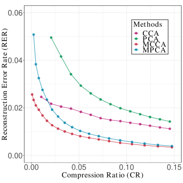
(a)

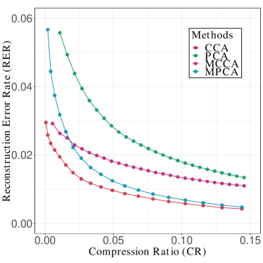
(b)

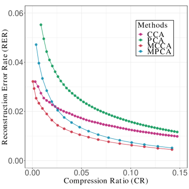
(c)

Fig. 1: Plots of RER versus CR for the AT&T(ORL) dataset of various group sizes: (a) Small; (b) Medium; and (c) Large.

6.3 Behavior of Contraction Ratio

We examined the behavior of contraction ratio $\alpha^{(k)}$. We performed MCCA on the AT&T(ORL) dataset with the medium group size and computed $\alpha^{(1)}$ and $\alpha^{(2)}$ with the various pairs of reduced dimensions $(R_{1},R_{2})\in\{1,2,\dots,25\}\times\{1,2,\dots,25\}$.

Figure 2 shows the values of $\alpha^{(1)}$ and $\alpha^{(2)}$ for all pairs of $R_{1}$ and $R_{2}$. As shown, $\alpha^{(1)}$ and $\alpha^{(2)}$ were invariant to variations in $R_{2}$ and $R_{1}$, respectively. Therefore, to facilitate visualization of changes in $\alpha^{(k)}$, Figure 3 shows $\alpha^{(1)}$ and $\alpha^{(2)}$ for, respectively, $R_{2}=1$ and $R_{1}=1$. From these, we observe that when both $R_{1}$ and $R_{2}$ are greater than 8, both $\alpha^{(1)}$ and $\alpha^{(2)}$ are close to one.

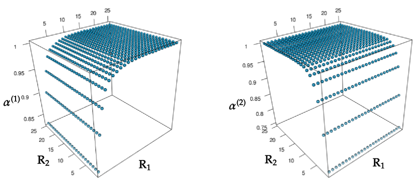
Fig. 2: $\alpha^{(1)}$ and $\alpha^{(2)}$ versus pairs of reduced dimensions $(R_{1},R_{2})$.

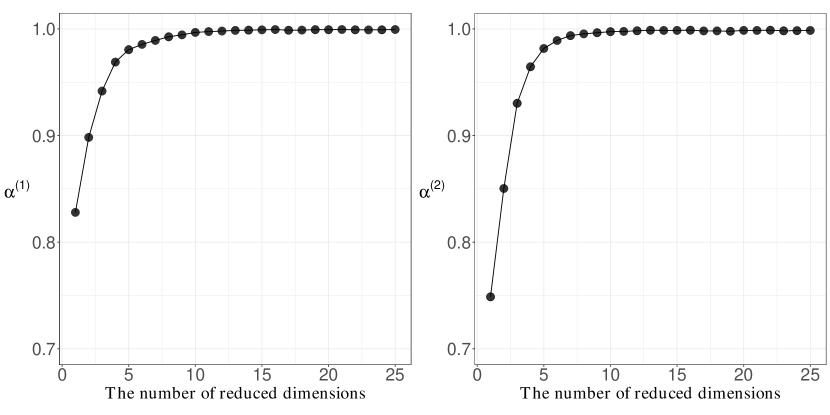
Fig. 3: $\alpha^{(1)}$ and $\alpha^{(2)}$ versus $R_{1}$ and $R_{2}$, respectively.

6.4 Efficacy of Solving the Quadratic Programming Problem

We investigated the usefulness of determining the initial value of $\bm{w}^{(k)}$ by solving the quadratic programming problem (4.1). We applied MCCA to the AT&T(ORL) dataset with the small, medium, and large number of groups. In addition, we also used the smaller group size of three. For determining the initial value of $\bm{w}^{(k)}$, we consider three methods: solving the quadratic programming problem (4.1) (MCCA:QP), setting all values of $\bm{w}^{(k)}$ to one (MCCA:FIX), and setting the values by random sampling according to the uniform distribution $U(0,1)$ (MCCA:RANDOM). We computed the $\alpha^{(k)}$ with the reduced dimensions $R_{1}=R_{2}\ (\in\quantity{1,2,\dots,10})$ for each of these methods.

To evaluate the performance of these methods, we compared the values of $\alpha^{(k)}$ and the number of iterations in the estimation. The number of iterations in the estimation is the number of repetitions of lines 7 to 9 in Algorithm 1. For MCCA(RANDOM), we performed 50 trials and calculated averages of each of these indices.

Figure 4 shows the comparisons of $\alpha^{(1)}$ and $\alpha^{(2)}$ when the initialization was performed by MCCA:QP, MCCA:FIX, and MCCA:RANDOM for AT&T(ORL) dataset with a group size of 3. It was confirmed that MCCA:QP provides the largest values of $\alpha^{(1)}$ and $\alpha^{(2)}$. Figure 5 shows that the number of iterations. MCCA:QP gives the smallest number of iterations for almost all values of the reduced dimensions. This result indicates that MCCA:QP converges to a solution faster than the other initialization methods. However, when the reduced dimension is greater than or equal to 8, the other methods are competitive with MCCA:QP. A lack of difference in the number of iterations could result from the closeness of the initial values and the global optimal solution. Note that when the $R_{1}$ and $R_{2}$ are greater than or equal to 8, $\alpha^{(1)}$ and $\alpha^{(2)}$ are sufficiently close to one, based on Figure 4. This indicates that the initial values are close to the global optimal solution obtained from Theorem 1. Hence, the result shows almost the same numbers of iterations for the three methods.

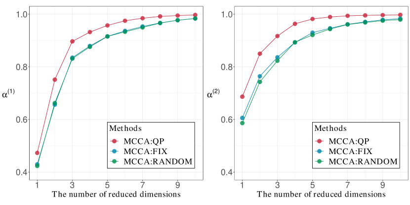
Fig. 4: Comparisons of $\alpha^{(1)}$ and $\alpha^{(2)}$ computed by using the initial values obtained from the initializations MCCA:QP, MCCA:FIX, and MCCA:RANDOM with the AT&T(ORL) dataset for a group size of 3.

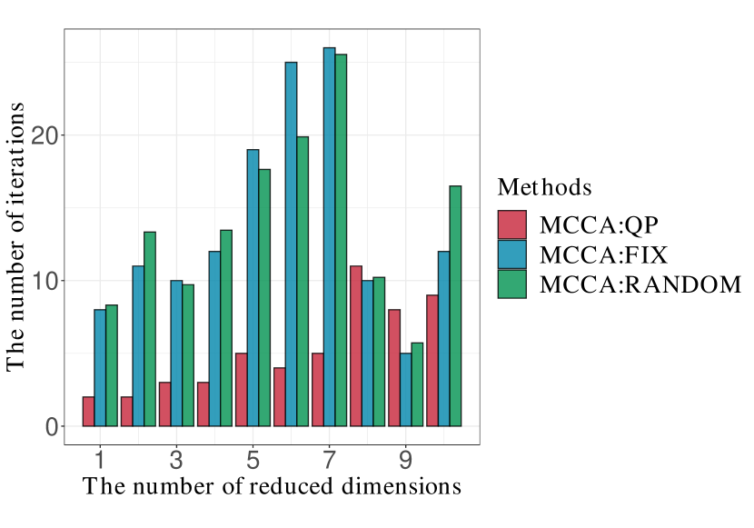
Fig. 5: Comparison of the number of iterations when the initialization was performed by MCCA:QP, MCCA:FIX, and MCCA:RANDOM with the AT&T(ORL) dataset for a group size of 3.

Figures 6 and 7 show comparisons for the AT&T(ORL) dataset with the medium group size. Since the figures for the results of other group sizes are similar to Figures 6 and 7, we show them in the supplementary mateirals S2.Figure 6 shows results similar those in Figure 4, whereas Figure 7 shows competitive performances for all reduced dimensions.

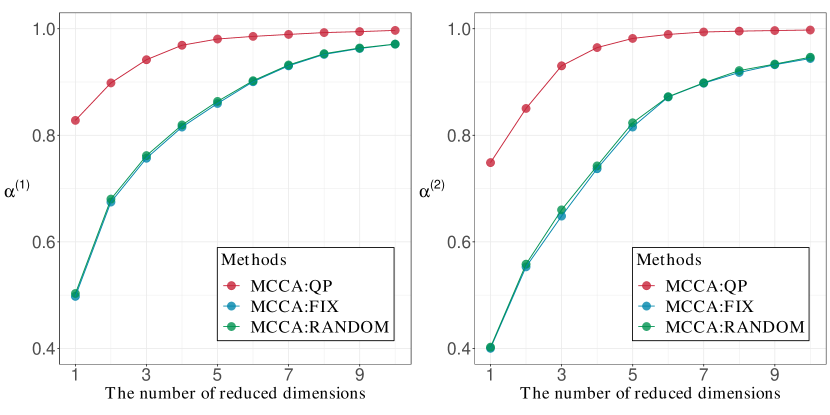
Fig. 6: Comparisons of $\alpha^{(1)}$ and $\alpha^{(2)}$ computed using the initial values obtained from the initialization of MCCA:QP, MCCA:FIX, and MCCA:RANDOM with the AT&T(ORL) dataset and the medium group size.

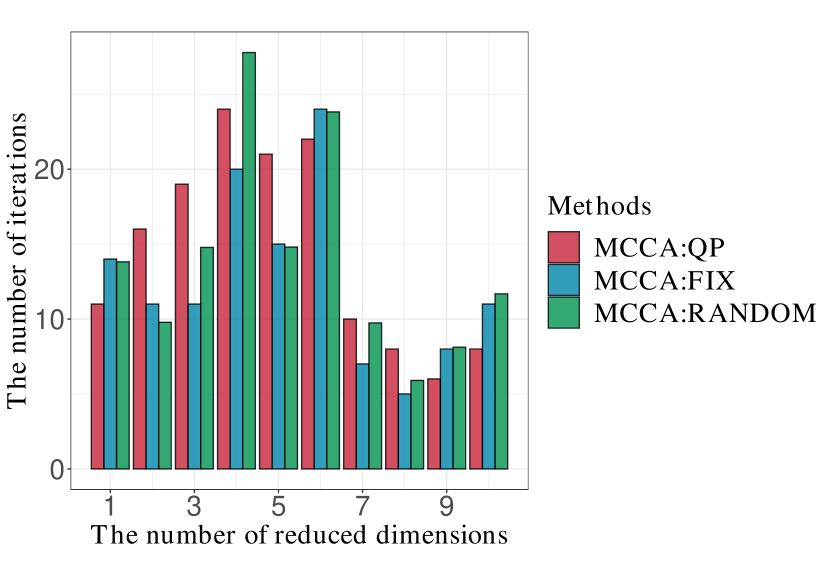
Fig. 7: Comparison of the number of iterations when the initialization was perfomed by MCCA:QP, MCCA:FIX, and MCCA:RANDOM with the AT&T(ORL) dataset and the medium group size.

7 Concluding Remarks

We have developed the multilinear common components analysis (MCCA) by introducing a covariance structure based on the Kronecker product. To efficiently solve the non-convex optimization problem for MCCA, we have proposed an iteratively updating algorithm. The proposed algorithm exhibits some superior theoretical convergence properties. Numerical experiments showed the usefulness of MCCA.

Specifically, MCCA was shown to be competitive among the initialization methods in terms of number of iterations. As the number of groups increases, the overall number of samples increases. This may be why all methods required almost the same number of iterations for small, medium, and large number of groups. Note that, in this study, we used the Kronecker product representation to estimate the covariance matrix for tensor datasets. Greenewald et al., (2019) used the Kronecker sum representation for estimating the covariance matrix, and it would be interesting to extend the MCCA to this and other covariance representations.

Appendices

Appendix A Proof of Lemma 1

We provide two lemmas about Kronecker products before we prove Lemma 1.

Lemma 2.

For matrices $\mathbf{A},\mathbf{B},\mathbf{C}$, and $\mathbf{D}$ such that matrix products $\mathbf{AC}$ and $\mathbf{BD}$ can be calculated,

$$(\mathbf{A}\otimes\mathbf{B})(\mathbf{C}\otimes\mathbf{D})=\mathbf{AC}\otimes\mathbf{BD}.$$

Lemma 3.

For square matrices $\mathbf{A}$ and $\mathbf{B}$,

$$\tr(\mathbf{A}\otimes\mathbf{B})=\tr(\mathbf{A})\tr(\mathbf{B}).$$

These lemmas are known as the mixed-product property and the spectrum property, respectively; see Harville, (1998) for detailed proofs.

Proof of Lemma 1:

For the maximization problem (3.5), move the summation over index $g$ out of the $\tr(\cdot)$ and replace $\mathbf{S}_{(g)}^{*}$ and $\mathbf{V}^{*}$ with $\mathbf{S}_{(g)}^{(1)}\otimes\mathbf{S}_{(g)}^{(2)}\otimes\cdots\otimes\mathbf{S}_{(g)}^{(M)}$ and $\mathbf{V}^{(1)}\otimes\mathbf{V}^{(2)}\otimes\cdots\otimes\mathbf{V}^{(M)}$, respectively. Then

$$\max_{\begin{subarray}{c}\mathbf{V}^{(k)}\\ k=1,2,\dots,M\end{subarray}}\sum_{g=1}^{G}\tr\left\{{\quantity(\mathbf{V}^{(1)}\otimes\cdots\otimes\mathbf{V}^{(M)})}^{\mathsf{T}}\quantity(\mathbf{S}_{(g)}^{(1)}\otimes\cdots\otimes\mathbf{S}_{(g)}^{(M)})\quantity(\mathbf{V}^{(1)}\otimes\cdots\otimes\mathbf{V}^{(M)})\right.$$

$$\left.{\quantity(\mathbf{V}^{(1)}\otimes\cdots\otimes\mathbf{V}^{(M)})}^{\mathsf{T}}\quantity(\mathbf{S}_{(g)}^{(1)}\otimes\cdots\otimes\mathbf{S}_{(g)}^{(M)})\quantity(\mathbf{V}^{(1)}\otimes\cdots\otimes\mathbf{V}^{(M)})\right\},$$

$$\mbox{\quad s.t.\quad}{\mathbf{V}^{(k)}}^{\mathsf{T}}\mathbf{V}^{(k)}=\mathbf{I}_{R_{k}}.$$

By Lemmas 2 and 3, we have

$$\max_{\begin{subarray}{c}{\mathbf{V}^{(k)}}^{\top}\mathbf{V}^{(k)}=\mathbf{I}_{R_{k}}\\ k=1,2,\dots,M\end{subarray}}\sum_{g=1}^{G}\tr\quantity{\quantity({\mathbf{V}^{(1)}}^{\top}\mathbf{S}_{(g)}^{(1)}\mathbf{V}^{(1)}{\mathbf{V}^{(1)}}^{\top}\mathbf{S}_{(g)}^{(1)}\mathbf{V}^{(1)})\cdots\quantity({\mathbf{V}^{(M)}}^{\top}\mathbf{S}_{(g)}^{(M)}\mathbf{V}^{(M)}{\mathbf{V}^{(M)}}^{\top}\mathbf{S}_{(g)}^{(M)}\mathbf{V}^{(M)})}$$

$$= \max_{\begin{subarray}{c}{\mathbf{V}^{(k)}}^{\top}\mathbf{V}^{(k)}=\mathbf{I}_{R_{k}}\\ k=1,2,\dots,M\end{subarray}}\sum_{g=1}^{G}\prod_{k=1}^{M}\tr\quantity{{\mathbf{V}^{(k)}}^{\mathsf{T}}\mathbf{S}_{(g)}^{(k)}\mathbf{V}^{(k)}{\mathbf{V}^{(k)}}^{\mathsf{T}}\mathbf{S}_{(g)}^{(k)}\mathbf{V}^{(k)}}.$$

This leads to the maximization problem in Lemma 1.

Appendix B Proof of Theorem 1

Theorem 1 can be easily shown from the following lemma.

Lemma 4.

Consider the maximization problem

$$\max_{\mathbf{V}^{(k)}}f_{k}^{\prime}({\mathbf{V}^{(k)}})=\max_{\mathbf{V}^{(k)}}\tr\quantity{{\mathbf{V}^{(k)}}^{\top}\quantity(\sum_{g=1}^{G}w_{(g)}^{(-k)}\mathbf{S}_{(g)}^{(k)}\mathbf{S}_{(g)}^{(k)})\mathbf{V}^{(k)}}.$$ (B.1)

Let $M^{(k)}=\tr\quantity{\sum_{g=1}^{G}w_{(g)}^{(-k)}\mathbf{S}_{(g)}^{(k)}\mathbf{S}_{(g)}^{(k)}}$. Then

$$\frac{f_{k}^{\prime}(\mathbf{V}^{(k)})^{2}}{M^{(k)}}\leq f_{k}(\mathbf{V}^{(k)})\leq f_{k}^{\prime}(\mathbf{V}^{(k)}).$$

Proof of Lemma 4:

First, we prove $f_{k}(\mathbf{V}^{(k)})\leq f_{k}^{\prime}(\mathbf{V}^{(k)})$. For any orthogonal matrix $\mathbf{V}^{(k)}\in\mathbb{R}^{P_{k}\times R_{k}}$, we can always find an orthogonal matrix $\mathbf{V}^{(k)}_{\bot}\in\mathbb{R}^{P_{k}\times(P_{k}-R_{k})}$ that satisfies $\mathbf{V}^{(k)\top}\mathbf{V}^{(k)}_{\bot}=\bm{O}$. Then the equation $\mathbf{V}^{(k)}{\mathbf{V}^{(k)}}^{\top}+\mathbf{V}^{(k)}_{\bot}{\mathbf{V}^{(k)}_{\bot}}^{\top}=\mathbf{I}_{P_{k}}$ holds. By definition,

$$f_{k}(\mathbf{V}^{(k)}) =\tr\quantity{{\mathbf{V}^{(k)}}^{\top}\quantity(\sum_{g=1}^{G}w_{(g)}^{(-k)}\mathbf{S}_{(g)}^{(k)}\mathbf{V}^{(k)}{\mathbf{V}^{(k)}}^{\top}\mathbf{S}_{(g)}^{(k)})\mathbf{V}^{(k)}}$$

$$\leq\tr\quantity{{\mathbf{V}^{(k)}}^{\top}\quantity(\sum_{g=1}^{G}w_{(g)}^{(-k)}\mathbf{S}_{(g)}^{(k)}\quantity(\mathbf{V}^{(k)}{\mathbf{V}^{(k)}}^{\top}+\mathbf{V}^{(k)}_{\bot}{\mathbf{V}^{(k)}_{\bot}}^{\top})\mathbf{S}_{(g)}^{(k)})\mathbf{V}^{(k)}}$$

$$=\tr\quantity{{\mathbf{V}^{(k)}}^{\top}\quantity(\sum_{g=1}^{G}w_{(g)}^{(-k)}\mathbf{S}_{(g)}^{(k)}\mathbf{S}_{(g)}^{(k)})\mathbf{V}^{(k)}}$$

$$=f_{k}^{\prime}({\mathbf{V}^{(k)}}).$$

Thus, we have obtained $f_{k}(\mathbf{V}^{(k)})\leq f_{k}^{\prime}({\mathbf{V}^{(k)}})$.

Next, we prove $\frac{f_{k}^{\prime}(\mathbf{V}^{(k)})^{2}}{M^{(k)}}\leq f_{k}(\mathbf{V}^{(k)})$. We define the following block matrices:

$$\mathbf{A} =\quantity[\sqrt{w_{(1)}^{(-k)}}{\mathbf{S}_{(1)}^{(k)}}^{\frac{1}{2}}\mathbf{V}^{(k)}{\mathbf{V}^{(k)}}^{\top}{\mathbf{S}_{(1)}^{(k)}}^{\frac{1}{2}},\dots,\sqrt{w_{(G)}^{(-k)}}{\mathbf{S}_{(G)}^{(k)}}^{\frac{1}{2}}\mathbf{V}^{(k)}{\mathbf{V}^{(k)}}^{\top}{\mathbf{S}_{(G)}^{(k)}}^{\frac{1}{2}}],$$

$$\mathbf{B} =\quantity[\sqrt{w_{(1)}^{(-k)}}\mathbf{S}_{(1)}^{(k)},\dots,\sqrt{w_{(G)}^{(-k)}}\mathbf{S}_{(G)}^{(k)}]$$

Note that since $\mathbf{S}_{(g)}^{(k)}$ is a symmetric positive definite matrix, $\mathbf{S}_{(g)}^{(k)}$ can be decomposed to ${\mathbf{S}_{(g)}^{(k)}}^{\frac{1}{2}}{\mathbf{S}_{(g)}^{(k)}}^{\frac{1}{2}}$. We calculate the traces of $\mathbf{A}\mathbf{A}$, $\mathbf{A}\mathbf{B}$, and $\mathbf{B}\mathbf{B}$, respectively:

$$\tr\quantity(\mathbf{A}\mathbf{A}) =\sum_{g=1}^{G}w_{(g)}^{(-k)}\tr\quantity({\mathbf{S}_{(g)}^{(k)}}^{\frac{1}{2}}\mathbf{V}^{(k)}{\mathbf{V}^{(k)}}^{\top}{\mathbf{S}_{(g)}^{(k)}}^{\frac{1}{2}}{\mathbf{S}_{(g)}^{(k)}}^{\frac{1}{2}}\mathbf{V}^{(k)}{\mathbf{V}^{(k)}}^{\top}{\mathbf{S}_{(g)}^{(k)}}^{\frac{1}{2}})$$

$$=\sum_{g=1}^{G}w_{(g)}^{(-k)}\tr\quantity{{\mathbf{V}^{(k)}}^{\top}\mathbf{S}_{(g)}^{(k)}\mathbf{V}^{(k)}{\mathbf{V}^{(k)}}^{\top}\mathbf{S}_{(g)}^{(k)}\mathbf{V}^{(k)}}$$

$$=\tr\quantity{{\mathbf{V}^{(k)}}^{\top}\quantity(\sum_{g=1}^{G}w_{(g)}^{(-k)}\mathbf{S}_{(g)}^{(k)}\mathbf{V}^{(k)}{\mathbf{V}^{(k)}}^{\top}\mathbf{S}_{(g)}^{(k)})\mathbf{V}^{(k)}}$$

$$=f_{k}(\mathbf{V}^{(k)}),$$

$$\tr\quantity(\mathbf{A}\mathbf{B}) =\sum_{g=1}^{G}w_{(g)}^{(-k)}\tr\quantity({\mathbf{S}_{(g)}^{(k)}}^{\frac{1}{2}}\mathbf{V}^{(k)}{\mathbf{V}^{(k)}}^{\top}{\mathbf{S}_{(g)}^{(k)}}^{\frac{1}{2}}\mathbf{S}_{(g)}^{(k)})$$

$$=\sum_{g=1}^{G}w_{(g)}^{(-k)}\tr\quantity({\mathbf{S}_{(g)}^{(k)}}^{\frac{1}{2}}\mathbf{V}^{(k)}{\mathbf{V}^{(k)}}^{\top}{\mathbf{S}_{(g)}^{(k)}}^{\frac{1}{2}}{\mathbf{S}_{(g)}^{(k)}}^{\frac{1}{2}}{\mathbf{S}_{(g)}^{(k)}}^{\frac{1}{2}})$$

$$=\sum_{g=1}^{G}w_{(g)}^{(-k)}\tr\quantity{{\mathbf{V}^{(k)}}^{\top}\mathbf{S}_{(g)}^{(k)}\mathbf{S}_{(g)}^{(k)}\mathbf{V}^{(k)}}$$

$$=\tr\quantity{{\mathbf{V}^{(k)}}^{\top}\quantity(\sum_{g=1}^{G}w_{(g)}^{(-k)}\mathbf{S}_{(g)}^{(k)}\mathbf{S}_{(g)}^{(k)})\mathbf{V}^{(k)}}$$

$$=f_{k}^{\prime}(\mathbf{V}^{(k)}),$$

$$\tr\quantity(\mathbf{B}\mathbf{B}) =\tr\quantity(\sum_{g=1}^{G}w_{(g)}^{(-k)}\mathbf{S}_{(g)}^{(k)}\mathbf{S}_{(g)}^{(k)})=M^{(k)}.$$

From the Cauchy–Schwarz inequality, we have

$$f_{k}(\mathbf{V}^{(k)})M^{(k)}=\tr\quantity(\mathbf{A}\mathbf{A})\tr\quantity(\mathbf{B}\mathbf{B})\geq\quantity{\tr\quantity(\mathbf{A}\mathbf{B})}^{2}=f_{k}^{\prime}(\mathbf{V}^{(k)})^{2}.$$

By dividing both sides of the inequality by $M^{(k)}$, we obtain $\frac{f_{k}^{\prime}(\mathbf{V}^{(k)})^{2}}{M^{(k)}}\leq f_{k}(\mathbf{V}^{(k)})$. This completes the proof.

∎

Proof of Theorem 1:

Let $f_{k}^{\prime\max}$ be the global maximum of $f_{k}^{\prime}(\mathbf{V}^{(k)})$ and $\mathbf{V}_{0}^{(k)}=\mathop{\rm arg~{}max}\limits_{\mathbf{V}^{(k)}}f_{k}^{\prime}(\mathbf{V}^{(k)})$. From Lemma 4 and the definition of $\alpha^{(k)}$, we have

$$\alpha^{(k)}f_{k}^{\prime\max}=\frac{f_{k}^{\prime}(\mathbf{V}_{0}^{(k)})^{2}}{M^{(k)}}\leq f_{k}(\mathbf{V}_{0}^{(k)}).$$

Let $f_{k}^{\max}$ be the global maximum of $f_{k}(\mathbf{V}^{(k)})$. It then holds that $f_{k}(\mathbf{V}_{0}^{(k)})\leq f_{k}^{\max}$. Thus

$$\alpha^{(k)}f_{k}^{\prime\max}\leq f_{k}^{\max}.$$

Let $\mathbf{V}_{0^{*}}^{(k)}=\mathop{\rm arg~{}max}\limits_{\mathbf{V}^{(k)}}f_{k}(\mathbf{V}^{(k)})$. From Lemma 4, we have

$$f_{k}^{\max}=f_{k}(\mathbf{V}_{0^{*}}^{(k)})\leq f_{k}^{\prime}(\mathbf{V}_{0^{*}}^{(k)}).$$

Since $f_{k}^{\prime}(\mathbf{V}_{0^{*}}^{(k)})\leq f_{k}^{\prime\max}$, we have

$$f_{k}^{\max}\leq f_{k}^{\prime\max}.$$

Hence, we have obtained $\alpha^{(k)}f_{k}^{\prime\max}\leq f_{k}^{\max}\leq f_{k}^{\prime\max}$.

∎

Appendix C Proof of Theorem 2

Proof of Theorem 2: By definition

$$\alpha^{(k)}=\frac{f_{k}^{\prime\max}}{M^{(k)}}=\frac{\tr\quantity{{{\mathbf{V}_{0}^{(k)}}}^{\top}\quantity(\sum_{g=1}^{G}w_{(g)}^{(-k)}\mathbf{S}_{(g)}^{(k)}\mathbf{S}_{(g)}^{(k)})\mathbf{V}_{0}^{(k)}}}{\tr\quantity{\sum_{g=1}^{G}w_{(g)}^{(-k)}\mathbf{S}_{(g)}^{(k)}\mathbf{S}_{(g)}^{(k)}}}.$$ (C.1)

By using the eigenvalue representation, we can rewrite the numerator of $\alpha^{(k)}$ as follows:

$$f_{k}^{\prime\max}=\sum_{g=1}^{G}w_{(g)}^{(-k)}\sum_{i=1}^{R_{k}}{\lambda_{(g)i}^{(k)}}.$$

On the other hand, the denominator of $\alpha^{(k)}$ can be represented as the sum of eigenvalues as follows:

$$M^{(k)}=\sum_{g=1}^{G}w_{(g)}^{(-k)}\sum_{i=1}^{P_{k}}{\lambda_{(g)i}^{(k)}}.$$

Thus, we can transform $\alpha^{(k)}$ as follows:

$$\alpha^{(k)}=\frac{\sum_{g=1}^{G}w_{(g)}^{(-k)}\sum_{i=1}^{R_{k}}{\lambda_{(g)i}^{(k)}}}{\sum_{g=1}^{G}w_{(g)}^{(-k)}\sum_{i=1}^{P_{k}}{\lambda_{(g)i}^{(k)}}}.$$

When we set

$$\bm{\lambda}_{0}^{(k)} =\quantity[\sum_{i=R_{k}+1}^{P_{k}}{\lambda_{(1)i}^{(k)}},\sum_{i=R_{k}+1}^{P_{k}}{\lambda_{(2)i}^{(k)}},\dots,\sum_{i=R_{k}+1}^{P_{k}}{\lambda_{(G)i}^{(k)}}]^{\top},$$

$$\bm{\lambda}_{1}^{(k)} =\quantity[\sum_{i=1}^{P_{k}}{\lambda_{(1)i}^{(k)}},\sum_{i=1}^{P_{k}}{\lambda_{(2)i}^{(k)}},\dots,\sum_{i=1}^{P_{k}}{\lambda_{(G)i}^{(k)}}]^{\top},$$

$$\bm{w}^{(k)} =\quantity[w_{(1)}^{(-k)},w_{(2)}^{(-k)},\dots,w_{(G)}^{(-k)}]^{\top},$$

we can reformulate $\alpha^{(k)}$ as

$$\alpha^{(k)}=\frac{\quantity(\bm{\lambda}_{1}^{(k)}-\bm{\lambda}_{0}^{(k)})^{\top}\bm{w}^{(k)}}{{\bm{\lambda}_{1}^{(k)}}^{\top}\bm{w}^{(k)}}.$$

Thus, we obtain the following maximization problem:

$$\max_{\bm{w}^{(k)}}\frac{\quantity(\bm{\lambda}_{1}^{(k)}-\bm{\lambda}_{0}^{(k)})^{\top}\bm{w}^{(k)}}{{\bm{\lambda}_{1}^{(k)}}^{\top}\bm{w}^{(k)}},\mbox{\quad s.t.\quad}\bm{w}^{(k)}>\bm{0}.$$

Note that the constraints can be obtained by the definition of $\bm{w}^{(k)}$. In addition, this maximization problem can be reformulated as

$$\max_{\bm{w}^{(k)}}\frac{\quantity(\bm{\lambda}_{1}^{(k)}-\bm{\lambda}_{0}^{(k)})^{\top}\bm{w}^{(k)}}{{\bm{\lambda}_{1}^{(k)}}^{\top}\bm{w}^{(k)}} =\max_{\bm{w}^{(k)}}1-\frac{{\bm{\lambda}_{0}^{(k)}}^{\top}\bm{w}^{(k)}}{{\bm{\lambda}_{1}^{(k)}}^{\top}\bm{w}^{(k)}}$$

$$=\min_{\bm{w}^{(k)}}\frac{{\bm{\lambda}_{0}^{(k)}}^{\top}\bm{w}^{(k)}}{{\bm{\lambda}_{1}^{(k)}}^{\top}\bm{w}^{(k)}}.$$

Since ${\bm{\lambda}_{0}^{(k)}}^{\top}\bm{w}^{(k)}/{\bm{\lambda}_{1}^{(k)}}^{\top}\bm{w}^{(k)}$ is non-negative, solving the optimization problem for the squared function of the objective function maintains generality. Thus, we can consider the following minimization problem:

$$\min_{\bm{w}^{(k)}}\frac{{\bm{w}^{(k)}}^{\top}\bm{\lambda}_{0}^{(k)}{\bm{\lambda}_{0}^{(k)}}^{\top}\bm{w}^{(k)}}{{\bm{w}^{(k)}}^{\top}\bm{\lambda}_{1}^{(k)}{\bm{\lambda}_{1}^{(k)}}^{\top}\bm{w}^{(k)}},\mbox{\quad s.t.\quad}\bm{w}^{(k)}>\bm{0}.$$

Additionally, from the invariance under multiplication of $\bm{w}^{(k)}$ by a constant, we obtain the following objective function of the quadratic programming problem.

$$\min_{\bm{w}^{(k)}}{\bm{w}^{(k)}}^{\top}\bm{\lambda}_{0}^{(k)}{\bm{\lambda}_{0}^{(k)}}^{\top}\bm{w}^{(k)},\mbox{\quad s.t.\quad}\bm{w}^{(k)}>\bm{0},\ {\bm{w}^{(k)}}^{\top}\bm{\lambda}_{1}^{(k)}{\bm{\lambda}_{1}^{(k)}}^{\top}\bm{w}^{(k)}=1.$$

The proof is complete.

∎

Appendix D Proof of Theorem 3

Proof of Theorem 3: We define the following block matrices:

$$\mathbf{A}_{s}=\quantity[\sqrt{w_{(1)}^{(-k)}}{\mathbf{S}_{(1)}^{(k)}}^{\frac{1}{2}}\mathbf{V}_{s}^{(k)}{\mathbf{V}_{s}^{(k)}}^{\top}{\mathbf{S}_{(1)}^{(k)}}^{\frac{1}{2}},\dots,\sqrt{w_{(G)}^{(-k)}}{\mathbf{S}_{(G)}^{(k)}}^{\frac{1}{2}}\mathbf{V}_{s}^{(k)}{\mathbf{V}_{s}^{(k)}}^{\top}{\mathbf{S}_{(G)}^{(k)}}^{\frac{1}{2}}].$$

Here, we calculate the traces of $\mathbf{A}_{s}\mathbf{A}_{s}$, $\mathbf{A}_{s}\mathbf{A}_{s+1}$, and $\mathbf{A}_{s+1}\mathbf{A}_{s+1}$. The calculations of $\tr\quantity(\mathbf{A}_{s}\mathbf{A}_{s})$ and $\tr\quantity(\mathbf{A}_{s+1}\mathbf{A}_{s+1})$ are the same as that of $\tr\quantity(\mathbf{A}\mathbf{A})$ by replacing $\mathbf{V}^{(k)}$ with $\mathbf{V}_{s}^{(k)}$ and $\mathbf{V}^{(k)}$ with $\mathbf{V}_{s+1}^{(k)}$, respectively, in Lemma 4. Thus, we obtain

$$\tr\quantity(\mathbf{A}_{s}\mathbf{A}_{s}) =f_{k}(\mathbf{V}_{s}^{(k)}),$$

$$\tr\quantity(\mathbf{A}_{s}\mathbf{A}_{s+1}) =\sum_{g=1}^{G}w_{(g)}^{(-k)}\tr\quantity({\mathbf{S}_{(g)}^{(k)}}^{\frac{1}{2}}\mathbf{V}_{s}^{(k)}{\mathbf{V}_{s}^{(k)}}^{\top}{\mathbf{S}_{(g)}^{(k)}}^{\frac{1}{2}}{\mathbf{S}_{(g)}^{(k)}}^{\frac{1}{2}}\mathbf{V}_{s+1}^{(k)}{\mathbf{V}_{s+1}^{(k)}}^{\top}{\mathbf{S}_{(g)}^{(k)}}^{\frac{1}{2}})$$

$$=\sum_{g=1}^{G}w_{(g)}^{(-k)}\tr\quantity{{\mathbf{V}_{s+1}^{(k)}}^{\top}\mathbf{S}_{(g)}^{(k)}\mathbf{V}_{s}^{(k)}{\mathbf{V}_{s}^{(k)}}^{\top}\mathbf{S}_{(g)}^{(k)}\mathbf{V}_{s+1}^{(k)}}$$

$$=\tr\quantity{{\mathbf{V}_{s+1}^{(k)}}^{\top}\quantity(\sum_{g=1}^{G}w_{(g)}^{(-k)}\mathbf{S}_{(g)}^{(k)}\mathbf{V}_{s}^{(k)}{\mathbf{V}_{s}^{(k)}}^{\top}\mathbf{S}_{(g)}^{(k)})\mathbf{V}_{s+1}^{(k)}},$$

$$\tr\quantity(\mathbf{A}_{s+1}\mathbf{A}_{s+1}) =f_{k}(\mathbf{V}_{s+1}^{(k)}).$$

Since $\mathbf{V}_{s+1}^{(k)}=\mathop{\rm arg~{}max}\limits_{\mathbf{V}^{(k)}}\tr\quantity{{\mathbf{V}^{(k)}}^{\top}\quantity(\sum_{g=1}^{G}w_{(g)}^{(-k)}\mathbf{S}_{(g)}^{(k)}\mathbf{V}_{s}^{(k)}{\mathbf{V}_{s}^{(k)}}^{\top}\mathbf{S}_{(g)}^{(k)})\mathbf{V}^{(k)}}$, we have

$$f_{k}(\mathbf{V}_{s}^{(k)}) =\tr\quantity{{\mathbf{V}_{s}^{(k)}}^{\top}\quantity(\sum_{g=1}^{G}w_{(g)}^{(-k)}\mathbf{S}_{(g)}^{(k)}\mathbf{V}_{s}^{(k)}{\mathbf{V}_{s}^{(k)}}^{\top}\mathbf{S}_{(g)}^{(k)})\mathbf{V}_{s}^{(k)}}$$

$$\leq\tr\quantity{{\mathbf{V}_{s+1}^{(k)}}^{\top}\quantity(\sum_{g=1}^{G}w_{(g)}^{(-k)}\mathbf{S}_{(g)}^{(k)}\mathbf{V}_{s}^{(k)}{\mathbf{V}_{s}^{(k)}}^{\top}\mathbf{S}_{(g)}^{(k)})\mathbf{V}_{s+1}^{(k)}}$$

$$=\tr\quantity(\mathbf{A}_{s}\mathbf{A}_{s+1}).$$

From the positivity of both sides of the inequality, it holds that

$$f_{k}(\mathbf{V}_{s}^{(k)})^{2}\leq\quantity[\tr\quantity(\mathbf{A}_{s}\mathbf{A}_{s+1})]^{2}.$$

In addition, from the Cauchy–Schwarz inequality, we have

$$f_{k}(\mathbf{V}_{s}^{(k)})f_{k}(\mathbf{V}_{s+1}^{(k)}) =\tr\quantity(\mathbf{A}_{s}\mathbf{A}_{s})\tr\quantity(\mathbf{A}_{s+1}\mathbf{A}_{s+1})$$

$$\geq\quantity[\tr\quantity(\mathbf{A}_{s}\mathbf{A}_{s+1})]^{2}.$$

Thus,

$$f_{k}(\mathbf{V}_{s}^{(k)})f_{k}(\mathbf{V}_{s+1}^{(k)})\geq\quantity[\tr\quantity(\mathbf{A}_{s}\mathbf{A}_{s+1})]^{2}\geq f_{k}(\mathbf{V}_{s}^{(k)})^{2}.$$

Thus, we have obtained $f_{k}(\mathbf{V}_{s}^{(k)})^{2}\leq f_{k}(\mathbf{V}_{s}^{(k)})f_{k}(\mathbf{V}_{s+1}^{(k)})$. By dividing both sides of the inequality by $f_{k}(\mathbf{V}_{s}^{(k)})$, we obtain the relation $f_{k}(\mathbf{V}_{s}^{(k)})\leq f_{k}(\mathbf{V}_{s+1}^{(k)})$.

∎

References

• Allen, (2012) Allen, G. (2012). Sparse higher-order principal components analysis. In Proceedings of the Fifteenth International Conference on Artificial Intelligence and Statistics, volume 22 of Proceedings of Machine Learning Research, pages 27–36.
• Badeau and Boyer, (2008) Badeau, R. and Boyer, R. (2008). Fast multilinear singular value decomposition for structured tensors. SIAM Journal on Matrix Analysis and Applications, 30(3):1008–1021.
• Bensmail and Celeux, (1996) Bensmail, H. and Celeux, G. (1996). Regularized gaussian discriminant analysis through eigenvalue decomposition. Journal of the American Statistical Association, 91(436):1743–1748.
• Boik, (2002) Boik, R. J. (2002). Spectral models for covariance matrices. Biometrika, 89(1):159–182.
• Carroll and Chang, (1970) Carroll, J. D. and Chang, J.-J. (1970). Analysis of individual differences in multidimensional scaling via an n-way generalization of “eckart-young” decomposition. Psychometrika, 35(3):283–319.
• Flury, (1984) Flury, B. N. (1984). Common principal components in k groups. Journal of the American Statistical Association, 79(388):892–898.
• Flury, (1986) Flury, B. N. (1986). Asymptotic theory for common principal component analysis. The Annals of Statistics, 14(2):418–430.
• Flury, (1988) Flury, B. N. (1988). Common principal components & related multivariate models. John Wiley & Sons, Inc.
• Flury and Gautschi, (1986) Flury, B. N. and Gautschi, W. (1986). An algorithm for simultaneous orthogonal transformation of several positive definite symmetric matrices to nearly diagonal form. SIAM Journal on Scientific and Statistical Computing, 7(1):169–184.
• Greenewald et al., (2019) Greenewald, K., Zhou, S., and Hero III, A. (2019). Tensor graphical lasso (teralasso). Journal of the Royal Statistical Society: Series B (Statistical Methodology), 81(5):901–931.
• Harshman, (1970) Harshman, R. A. (1970). Foundations of the PARAFAC procedure : Models and conditions for an ”explanatory” multimodal factor analysis. UCLA Working Papers in Phonetics, 16(1):84.
• Harville, (1998) Harville, D. A. (1998). Matrix Algebra From a Statistician’s Perspective. Springer-Verlag, New York.
• Jolliffe, (2002) Jolliffe, I. (2002). Principal Component Analysis. Springer-Verlag, New York.
• Kermoal et al., (2002) Kermoal, J. P., Schumacher, L., Pedersen, K. I., Mogensen, P. E., and Frederiksen, F. (2002). A stochastic mimo radio channel model with experimental validation. IEEE Journal on Selected Areas in Communications, 20(6):1211–1226.
• Kiers, (2000) Kiers, H. A. (2000). Towards a standardized notation and terminology in multiway analysis. Journal of Chemometrics: A Journal of the Chemometrics Society, 14(3):105–122.
• Kolda and Bader, (2009) Kolda, T. G. and Bader, B. W. (2009). Tensor decompositions and applications. SIAM review, 51(3):455–500.
• Lai et al., (2014) Lai, Z., Xu, Y., Chen, Q., Yang, J., and Zhang, D. (2014). Multilinear sparse principal component analysis. IEEE Transactions on Neural Networks and Learning Systems, 25(10):1942–1950.
• Lecun et al., (1998) Lecun, Y., Bottou, L., Bengio, Y., and Haffner, P. (1998). Gradient-based learning applied to document recognition. Proceedings of the IEEE, 86(11):2278–2324.
• Lu et al., (2008) Lu, H., Plataniotis, K. N., and Venetsanopoulos, A. N. (2008). MPCA: Multilinear principal component analysis of tensor objects. IEEE transactions on Neural Networks, 19(1):18–39.
• Manly and Rayner, (1987) Manly, B. F. J. and Rayner, J. C. W. (1987). The comparison of sample covariance matrices using likelihood ratio tests. Biometrika, 74(4):841–847.
• Martinez and Benavente., (1998) Martinez, A. and Benavente., R. (1998). The AR face database. CVC Technical Report, 24.
• Martinez and Kak, (2001) Martinez, A. M. and Kak, A. C. (2001). PCA versus LDA. IEEE Transactions on Pattern Analysis and Machine Intelligence, 23(2):228–233.
• Park and Konishi, (2018) Park, H. and Konishi, S. (2018). Sparse common component analysis for multiple high-dimensional datasets via noncentered principal component analysis. Statistical Papers.
• Pearson, (1901) Pearson, K. (1901). LIII. On lines and planes of closest fit to systems of points in space. The London, Edinburgh, and Dublin Philosophical Magazine and Journal of Science, 2(11):559–572.
• Pourahmadi et al., (2007) Pourahmadi, M., Daniels, M. J., and Park, T. (2007). Simultaneous modelling of the cholesky decomposition of several covariance matrices. Journal of Multivariate Analysis, 98(3):568–587.
• R Core Team, (2019) R Core Team (2019). R: A Language and Environment for Statistical Computing. R Foundation for Statistical Computing, Vienna, Austria.
• Wang et al., (2011) Wang, H., Banerjee, A., and Boley, D. (2011). Common component analysis for multiple covariance matrices. In Proceedings of the 17th ACM SIGKDD International Conference on Knowledge Discovery and Data Mining, pages 956–964.
• Wang et al., (2012) Wang, S., Sun, M., Chen, Y., Pang, E., and Zhou, C. (2012). STPCA: Sparse tensor Principal Component Analysis for feature extraction. In Proceedings of the 21st International Conference on Pattern Recognition (ICPR2012), pages 2278–2281.
• Werner et al., (2008) Werner, K., Jansson, M., and Stoica, P. (2008). On estimation of covariance matrices with kronecker product structure. IEEE Transactions on Signal Processing, 56(2):478–491.
• Yu et al., (2004) Yu, K., Bengtsson, M., Ottersten, B., McNamara, D., Karlsson, P., and Beach, M. (2004). Modeling of wide-band mimo radio channels based on nlos indoor measurements. IEEE Transactions on Vehicular Technology, 53(3):655–665.